111/3/2016

36-463/663: Hierarchical

Linear Models

Taste of MCMC / Bayes for 3 or more “levels”

Brian Junker

132E Baker Hall

brian@stat.cmu.edu

211/3/2016

Outline

� Practical Bayes

� Mastery Learning Example

� A brief taste of JAGS and RUBE

� Hierarchical Form of Bayesian Models

� Extending the “Levels” and the “Slogan”

� Mastery Learning – Distribution of “mastery”

� (to be continued…)

311/3/2016

Practical Bayesian Statistics

� (posterior) ∝ (likelihood)×(prior)

� We typically want quantities like

� point estimate: Posterior mean, median, mode

� uncertainty: SE, IQR, or other measure of ‘spread’

� credible interval (CI)

� (θ - 2SE, θ + 2SE)

� (θ. , θ.)

� Other aspects of the “shape” of the posterior distribution

� Aside: If (prior) ∝ 1, then

� (posterior) ∝ (likelihood)

� posterior mode = mle, posterior SE = 1/I(θ)1/2, etc.

^ ^

411/3/2016

Obtaining posterior point estimates,

credible intervals

� Easy if we recognize the posterior distribution and we have formulae for means, variances, etc.

� Whether or not we have such formulae, we can get similar information by simulating from the posterior distribution.

� Key idea:

where θ, θ, …, θM is a sample from f(θ|data).

511/3/2016

Example: Mastery Learning

� Some computer-based tutoring systems declare that you have “mastered” a skill if you can perform it successfully r times.

� The number of times x that you erroneously perform the skill before the rth success is a measure of how likely you are to perform the skill correctly (how well you know the skill).

� The distribution for the number of failures x before the rth success is the negative binomial distribution.

611/3/2016

Negative Binomial Distribution

� Let X = x, the number of failures before the rth

success. The negative binomial distribution is

� The conjugate prior distribution is the beta

distribution

711/3/2016

Posterior inference for negative

binomial and beta prior

� (posterior) ∝ (likelihood)×(prior):

� Since this is Beta(p|α+r,β+x),

� and this lets us compute point estimate and approximate 95% CI’s.

811/3/2016

Some specific cases…� Let α = 1, β = 1 (so the prior is Unif(0,1)), and suppose

we declare mastery for 3 successes

� If X = 4, then

Approx 95% CI: (0.12, 0.76)

� If X = 10, then

Approx 95% CI: (0.05, 0.49)

911/3/2016

We can get similar answers with

simulation� When X = 4, r = 3, α + r = 4, β + x = 5

> p.post <- rbeta(10000,4,5)

> mean(p.post)

[1] 0.4444919

> var(p.post)

[1] 0.02461883

> quantile(p.post,c(0.025,0.975))

2.5% 97.5%

0.1605145 0.7572414

> plot(density(p.post))

� When X = 10, r = 3, α + r = 4, β + x = 11> p.post <- rbeta(10000,4,11)

> mean(p.post)

[1] 0.2651332

> var(p.post)

[1] 0.01201078

> quantile(p.post,c(0.025,0.975))

2.5% 97.5%

0.0846486 0.5099205

> plot(density(p.post))

0.0 0.2 0.4 0.6 0.8 1.0

0.0

0.5

1.0

1.5

2.0

density.default(x = p.post)

N = 10000 Bandwidth = 0.02238

De

nsity

0.0 0.2 0.4 0.6 0.8

0.0

0.5

1.0

1.5

2.0

2.5

3.0

3.5

density.default(x = p.post)

N = 10000 Bandwidth = 0.01563

Den

sity

1011/3/2016

Using a non-conjugate prior distribution

� Instead of a uniform prior, suppose psychological theory

says the prior density should increase linearly from 0.5

to 1.5 as θ moves from 0 to 1?

0.0 0.2 0.4 0.6 0.8 1.0

0.0

0.5

1.0

1.5

θ

uniform density

0.0 0.2 0.4 0.6 0.8 1.0

0.0

0.5

1.0

1.5

θ

linear density

1111/3/2016

Posterior inference for negative

binomial and linear prior

� (posterior) ∝ (likelihood)×(prior):

� r = 3, x = 4:

� r = 3, x = 10:

1211/3/2016

What to do with ?

� No formulae for means, variances!

� No nice function in R for simulation!

� There are many simulation methods that we can build “from scratch”

� B. Ripley (1981) Stochastic Simulation, Wiley.

� L. Devroye (1986) Nonuniform random variate generation, Springer.

� We will focus on just one method:

� Markov Chain Monte Carlo (MCMC)

� Programs like WinBUGS and JAGS automate the simulation/sampling method for us.

We will use this to give a taste of

JAGS… Need likelihood and prior:� Likelihood is easy:

x ~ dnegbin(p,r)

� Prior for p is a little tricky:

p ~ f(p) = p + 0.5 not a standard density!

� But we can use a trick:

the inverse probability transform

1311/3/2016

Aside: the Inverse Probability

Transform� If U ~ Unif(0,1) and F(z) is the CDF of a continuous

random variable, then Z = F-1(U) will have F(z) as

its CDF (exercise!!).

� The prior for p in our model has pdf p + 1/2, so its

CDF is F(p)=(p2 + p)/2.

� F-1(u) = (2u + 1/4)1/2 – 1/2

� So if U ~ Unif(0,1), then

P = (2U + 1/4)1/2 – 1/2

has density f(p) = p + 1/2.

1411/3/2016

JAGS: Need to specify likelihood and

prior� Likelihood is easy:

x ~ dnegbin(p,r)

� Prior for p is:

p <- (u + 1/4)^{1/2} + 1/2

where

u ~ dunif(0,1)

1511/3/2016

The JAGS model

mastery.learning.model <- "model {

# specify the number of successes needed for mastery

r <- 3

# specify likelihood

x ~ dnegbin(p,r)

# specify prior (using inverse probability xform)

p <- sqrt(2*u + 0.25) - 0.5

u ~ dunif(0,1)

}"

1611/3/2016

Estimate p when student has 4

failures before 3 successes> library(R2jags)

> library(rube)

> mastery.data <- list(x=4)

> rube.fit <- rube(mastery.learning.model,

+ mastery.data, mastery.init,

+ parameters.to.save=c("p"),

+ n.iter=20000,n.thin=3)

> # generates about 10,000 samples

> p <- rube.fit$sims.list$p

> hist(p,prob=T)

> lines(density(p))

> mean(p) + c(-2,0,2)*sd(p)

[1] 0.1549460 0.4685989 0.7822518

> quantile(p,c(0.025, 0.50, 0.975))

2.5% 50% 97.5%

0.1777994 0.4661076 0.7801111

1711/3/2016

Estimate p when student has 10

failures before 3 successes

1811/3/2016

> # library(R2jags)

> # library(rube)

> mastery.data <- list(x=10)

> rube.fit <- rube(mastery.learning.model,

+ mastery.data, mastery.init,

+ parameters.to.save=c("p"),

+ n.iter=20000,n.thin=3)

> # generates about 10,000 samples

> p <- rube.fit$sims.list$p

> hist(p,prob=T)

> lines(density(p))

> mean(p) + c(-2,0,2)*sd(p)

[1] 0.05594477 0.28247419 0.50900361

> quantile(p,c(0.025, 0.50, 0.975))

2.5% 50% 97.5%

0.09085802 0.27119223 0.52657339

1911/3/2016

Hierarchical Form of Bayesian Models

� In the past few lectures, we’ve seen many models

that involve a likelihood and a prior

� A somewhat more compact notation is used to

describe the models, and we will start using it

now

� Level 1: the likelihood (the distribution of the data)

� Level 2: the prior (the distribution of the parameter(s))

� Eventually there will be other levels as well!

� Examples on the following pages…

2011/3/2016

Hierarchical Beta-Binomial model

� Likelihood is binomial:

� Prior is beta distribution:

� (posterior) ∝

(likelihood)×(prior)

� Level 1: x ~ Binom(x|n,p)

� Level 2: p ~ Beta(p|α,β)

� (posterior) ∝

(level 1)×(level 2)

= Beta(p|α+x,β+n-x)

2111/3/2016

Hierarchical Gamma-Exponential Model

� Likelihood is Exponential:

� Prior is Gamma:

� (posterior) ∝

(likelihood)×(prior)

� Level 1:

� Level 2:

� (posterior) ∝

(level 1)×(level 2)

= Gamma(λ|α+n,β + n x)

2211/3/2016

Hierarchical Normal-Normal model

� Likelihood (for mean) is normal:

� Prior is normal (for mean):

� (posterior) ∝(likelihood)×(prior)

� Level 1:

� Level 2:

� (posterior)∝

(level 1)×(level 2)

2311/3/2016

Hierarchical Beta-Negative Binomial

Model

� Likelihood is Negative-

Binomial:

� Prior is Gamma:

� (posterior)∝

(likelihood)×(prior)

� Level 1:

� Level 2:

� (posterior)∝

(level 1)×(level 2)

2411/3/2016

Hierarchical Linear-Negative Binomial

Model

� Likelihood is Negative-

Binomial:

� Prior is Linear Density:

� (posterior)∝

(likelihood)×(prior)

� Level 1:

� Level 2:

� (posterior)∝

(level 1)×(level 2)

2511/3/2016

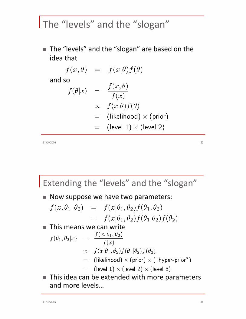
The “levels” and the “slogan”

� The “levels” and the “slogan” are based on the

idea that

and so

2611/3/2016

Extending the “levels” and the “slogan”

� Now suppose we have two parameters:

� This means we can write

� This idea can be extended with more parameters and more levels…

2711/3/2016

Mastery Learning: Distribution of

Masteries� Last time, we considered one student at a time according

to� Level 1: x ∼ NB(x|r,p)

� Level 2: p ∼ Beta(p|α,β)

� Now, suppose we have a sample of n students, and the number of failures before the rth success for each student is x1, x2, …, xn. � We want to know the distribution of p, the probability of success,

in the population: i.e. we want to estimate α & β !

� We will model this as� Level 1: xi ∼ NB(x|r,pi), i=1, …, n

� Level 2: pi ∼ Beta(p|α,β) , i = 1, …, n

� Level 3: α∼ Gamma(α|a1,b1), β ∼ Gamma(β|a2,b2)

2811/3/2016

Mastery Learning: Distribution of

Masteries

� We want to know the distribution of p, the

probability of success, in the population: i.e. we

want to estimate α & β !

� Level 1: xi ∼ NB(x|r,pi), i=1, …, n

� Level 2: pi ∼ Beta(p|α,β), i = 1, …, n

� Level 3: α∼ Gamma(α|a1,b1), β ∼ Gamma(α|a2,b2)

α,β for population of students

pi = student prob of right

xi = errors before r rights

n+2 parameters!

2911/3/2016

Mastery Learning: Distribution of

Masteries

� Level 1: If x1, x2, … xn are the failure counts then

� Level 2: If p1, p2, … pn are the success probabilties,

� Level 3:

3011/3/2016

Distribution of Mastery probabilities…

� Applying the “slogan” for 3 levels:

We can drop these

since they only

depend on data

Can’t drop these

since we want to est α & β…

We need to choose a1, b1,a2, b2. Then we can drop these

3111/3/2016

Distribution of Mastery probabilities…

� If we take a1=1, b1=1, a2=1, b2=1, and drop the constants we can drop, we get

� Suppose our data consist of the n=5 values

x1 = 4, x2 = 10, x3=5, x4 = 7, x5 = 3

(number of failures before r=3 successes)

� Problem: We need a way to sample from the 5+2=7 parameters p1, …, p5, α, β!

3211/3/2016

Solution: Markov-Chain Monte Carlo

(MCMC)

� MCMC is very useful for multivariate distributions, e.g. f(θ,θ, …,θK)

� Instead of dreaming up a way to make a draw (simulation) of all K variables at once MCMC takes draws one at a time

� We “pay” for this by not getting independent draws. The draws are the states of a Markov Chain.

� The draws will not be “exactly right” right away; the Markov chain has to “burn in” to a stationary distribution; the draws after the “burn-in” are what we want!

For theory, see Chib & Greenberg, American Statistician, 1995, pp. 327-335

3311/3/2016

Summary

� Practical Bayes

� Mastery Learning Example

� A brief taste of JAGS and RUBE

� Hierarchical Form of Bayesian Models

� Extending the “Levels” and the “Slogan”

� Mastery Learning – Distribution of “mastery”

� (to be continued…)