3 Basics of Bayesian Statistics - Carnegie Mellon Universitybrian/463-663/week09/Chapter 03.pdf ·...

3

Basics of Bayesian Statistics

Suppose a woman believes she may be pregnant after a single sexual encounter,but she is unsure. So, she takes a pregnancy test that is known to be 90%accurate—meaning it gives positive results to positive cases 90% of the time—and the test produces a positive result.1 Ultimately, she would like to know theprobability she is pregnant, given a positive test (p(preg | test +)); however,what she knows is the probability of obtaining a positive test result if she ispregnant (p(test + |preg)), and she knows the result of the test.

In a similar type of problem, suppose a 30-year-old man has a positiveblood test for a prostate cancer marker (PSA). Assume this test is also ap-proximately 90% accurate. Once again, in this situation, the individual wouldlike to know the probability that he has prostate cancer, given the positivetest, but the information at hand is simply the probability of testing positiveif he has prostate cancer, coupled with the knowledge that he tested positive.

Bayes’ Theorem offers a way to reverse conditional probabilities and,hence, provides a way to answer these questions. In this chapter, I first showhow Bayes’ Theorem can be applied to answer these questions, but then Iexpand the discussion to show how the theorem can be applied to probabilitydistributions to answer the type of questions that social scientists commonlyask. For that, I return to the polling data described in the previous chapter.

3.1 Bayes’ Theorem for point probabilities

Bayes’ original theorem applied to point probabilities. The basic theoremstates simply:

p(B|A) =p(A|B)p(B)

p(A). (3.1)

1 In fact, most pregnancy tests today have a higher accuracy rate, but the accuracyrate depends on the proper use of the test as well as other factors.

48 3 Basics of Bayesian Statistics

In English, the theorem says that a conditional probability for event Bgiven event A is equal to the conditional probability of event A given eventB, multiplied by the marginal probability for event B and divided by themarginal probability for event A.

Proof: From the probability rules introduced in Chapter 2, we know thatp(A,B) = p(A|B)p(B). Similarly, we can state that p(B,A) = p(B|A)p(A).Obviously, p(A,B) = p(B,A), so we can set the right sides of each of theseequations equal to each other to obtain:

p(B|A)p(A) = p(A|B)p(B).

Dividing both sides by p(A) leaves us with Equation 3.1.The left side of Equation 3.1 is the conditional probability in which we

are interested, whereas the right side consists of three components. p(A|B)is the conditional probability we are interested in reversing. p(B) is the un-conditional (marginal) probability of the event of interest. Finally, p(A) is themarginal probability of event A. This quantity is computed as the sum ofthe conditional probability of A under all possible events Bi in the samplespace: Either the woman is pregnant or she is not. Stated mathematically fora discrete sample space:

p(A) =∑

Bi∈SB

p(A | Bi)p(Bi).

Returning to the pregnancy example to make the theorem more concrete,suppose that, in addition to the 90% accuracy rate, we also know that thetest gives false-positive results 50% of the time. In other words, in cases inwhich a woman is not pregnant, she will test positive 50% of the time. Thus,there are two possible events Bi: B1 = preg and B2 = not preg. Additionally,given the accuracy and false-positive rates, we know the conditional probabil-ities of obtaining a positive test under these events: p(test +|preg) = .9 andp(test +|not preg) = .5. With this information, combined with some “prior”information concerning the probability of becoming pregnant from a singlesexual encounter, Bayes’ theorem provides a prescription for determining theprobability of interest.

The “prior” information we need, p(B) ≡ p(preg), is the marginal probabil-ity of being pregnant, not knowing anything beyond the fact that the womanhas had a single sexual encounter. This information is considered prior infor-mation, because it is relevant information that exists prior to the test. We mayknow from previous research that, without any additional information (e.g.,concerning date of last menstrual cycle), the probability of conception for anysingle sexual encounter is approximately 15%. (In a similar fashion, concerningthe prostate cancer scenario, we may know that the prostate cancer incidencerate for 30-year-olds is .00001—see Exercises). With this information, we candetermine p(B | A) ≡ p(preg|test +) as:

3.1 Bayes’ Theorem for point probabilities 49

p(preg | test +) =p(test + | preg)p(preg)

p(test + | preg)p(preg) + p(test + | not preg)p(not preg).

Filling in the known information yields:

p(preg | test +) =(.90)(.15)

(.90)(.15) + (.50)(.85)=

.135

.135 + .425= .241.

Thus, the probability the woman is pregnant, given the positive test, is only.241. Using Bayesian terminology, this probability is called a “posterior prob-ability,” because it is the estimated probability of being pregnant obtainedafter observing the data (the positive test). The posterior probability is quitesmall, which is surprising, given a test with so-called 90% “accuracy.” How-ever, a few things affect this probability. First is the relatively low probabilityof becoming pregnant from a single sexual encounter (.15). Second is the ex-tremely high probability of a false-positive test (.50), especially given the highprobability of not becoming pregnant from a single sexual encounter (p = .85)(see Exercises).

If the woman is aware of the test’s limitations, she may choose to repeat thetest. Now, she can use the “updated” probability of being pregnant (p = .241)as the new p(B); that is, the prior probability for being pregnant has now beenupdated to reflect the results of the first test. If she repeats the test and againobserves a positive result, her new “posterior probability” of being pregnantis:

p(preg | test +) =(.90)(.241)

(.90)(.241) + (.50)(.759)=

.135

.135 + .425= .364.

This result is still not very convincing evidence that she is pregnant, but if sherepeats the test again and finds a positive result, her probability increases to.507 (for general interest, subsequent positive tests yield the following prob-abilities: test 4 = .649, test 5 = .769, test 6 = .857, test 7 = .915, test 8 =.951, test 9 = .972, test 10 = .984).

This process of repeating the test and recomputing the probability of in-terest is the basic process of concern in Bayesian statistics. From a Bayesianperspective, we begin with some prior probability for some event, and we up-date this prior probability with new information to obtain a posterior prob-ability. The posterior probability can then be used as a prior probability ina subsequent analysis. From a Bayesian point of view, this is an appropriatestrategy for conducting scientific research: We continue to gather data to eval-uate a particular scientific hypothesis; we do not begin anew (ignorant) eachtime we attempt to answer a hypothesis, because previous research providesus with a priori information concerning the merit of the hypothesis.


3.2 Bayes’ Theorem applied to probability distributions

Bayes’ theorem, and indeed, its repeated application in cases such as the ex-ample above, is beyond mathematical dispute. However, Bayesian statisticstypically involves using probability distributions rather than point probabili-ties for the quantities in the theorem. In the pregnancy example, we assumedthe prior probability for pregnancy was a known quantity of exactly .15. How-ever, it is unreasonable to believe that this probability of .15 is in fact thisprecise. A cursory glance at various websites, for example, reveals a wide rangefor this probability, depending on a woman’s age, the date of her last men-strual cycle, her use of contraception, etc. Perhaps even more importantly,even if these factors were not relevant in determining the prior probabilityfor being pregnant, our knowledge of this prior probability is not likely to beperfect because it is simply derived from previous samples and is not a knownand fixed population quantity (which is precisely why different sources maygive different estimates of this prior probability!). From a Bayesian perspec-tive, then, we may replace this value of .15 with a distribution for the priorpregnancy probability that captures our prior uncertainty about its true value.The inclusion of a prior probability distribution ultimately produces a poste-rior probability that is also no longer a single quantity; instead, the posteriorbecomes a probability distribution as well. This distribution combines theinformation from the positive test with the prior probability distribution toprovide an updated distribution concerning our knowledge of the probabilitythe woman is pregnant.

Put generally, the goal of Bayesian statistics is to represent prior uncer-tainty about model parameters with a probability distribution and to updatethis prior uncertainty with current data to produce a posterior probability dis-tribution for the parameter that contains less uncertainty. This perspectiveimplies a subjective view of probability—probability represents uncertainty—and it contrasts with the classical perspective. From the Bayesian perspective,any quantity for which the true value is uncertain, including model param-eters, can be represented with probability distributions. From the classicalperspective, however, it is unacceptable to place probability distributions onparameters, because parameters are assumed to be fixed quantities: Only thedata are random, and thus, probability distributions can only be used to rep-resent the data.

Bayes’ Theorem, expressed in terms of probability distributions, appearsas:

f(θ|data) =f(data|θ)f(θ)

f(data), (3.2)

where f(θ|data) is the posterior distribution for the parameter θ, f(data|θ)is the sampling density for the data—which is proportional to the Likeli-hood function, only differing by a constant that makes it a proper densityfunction—f(θ) is the prior distribution for the parameter, and f(data) is the

3.2 Bayes’ Theorem applied to probability distributions 51

marginal probability of the data. For a continuous sample space, this marginalprobability is computed as:

f(data) =

∫

f(data|θ)f(θ)dθ,

the integral of the sampling density multiplied by the prior over the samplespace for θ. This quantity is sometimes called the “marginal likelihood” for thedata and acts as a normalizing constant to make the posterior density proper(but see Raftery 1995 for an important use of this marginal likelihood). Be-cause this denominator simply scales the posterior density to make it a properdensity, and because the sampling density is proportional to the likelihoodfunction, Bayes’ Theorem for probability distributions is often stated as:

Posterior ∝ Likelihood× Prior, (3.3)

where the symbol “∝” means “is proportional to.”

3.2.1 Proportionality

As Equation 3.3 shows, the posterior density is proportional to the likelihoodfunction for the data (given the model parameters) multiplied by the prior forthe parameters. The prior distribution is often—but not always—normalizedso that it is a true density function for the parameter. The likelihood function,however, as we saw in the previous chapter, is not itself a density; instead, it isa product of densities and thus lacks a normalizing constant to make it a truedensity function. Consider, for example, the Bernoulli versus binomial speci-fications of the likelihood function for the dichotomous voting data. First, theBernoulli specification lacked the combinatorial expression to make the like-lihood function a true density function for either the data or the parameter.Second, although the binomial representation for the likelihood function con-stituted a true density function, it only constituted a true density for the data

and not for the parameter p. Thus, when the prior distribution for a parameteris multiplied by the likelihood function, the result is also not a proper densityfunction. Indeed, Equation 3.3 will be “off” by the denominator on the rightside of Equation 3.2, in addition to whatever normalizing constant is neededto equalize the likelihood function and the sampling density p(data | θ).

Fortunately, the fact that the posterior density is only proportional to theproduct of the likelihood function and prior is not generally a problem inBayesian analysis, as the remainder of the book will demonstrate. However,a note is in order regarding what proportionality actually means. In brief, ifa is proportional to b, then a and b only differ by a multiplicative constant.How does this translate to probability distributions? First, we need to keep inmind that, in a Bayesian analysis, model parameters are considered randomquantities, whereas the data, having been already observed, are consideredfixed quantities. This view is completely opposite that assumed under the


classical approach. Second, we need to recall from Chapter 2 that potentialdensity functions often need to have a normalizing constant included to makethem proper density functions, but we also need to recall that this normalzingconstant only has the effect of scaling the density—it does not fundamentallychange the relative frequencies of different values of the random variable.As we saw in Chapter 2, the normalizing constant is sometimes simply atrue constant—a number—but sometimes the constant involves the randomvariable(s) themselves.

As a general rule, when considering a univariate density, any term, sayQ (no matter how complicated), that can be factored away from the randomvariable in the density—so that all the term(s) involving the random variableare simply multiples of Q—can be considered an irrelevant proportionalityconstant and can be eliminated from the density without affecting the results.

In theory, this rule is fairly straightforward, but it is often difficult to applyfor two key reasons. First, it is sometimes difficult to see whether a term canbe factored out. For example, consider the following function for θ:

f(θ) = e−θ+Q.

It may not be immediately clear that Q here is an arbitrary constant withrespect to θ, but it is. This function can be rewritten as:

f(θ) = e−θ × eQ,

using the algebraic rule that ea+b = eaeb. Thus, if we are considering f(θ)as a density function for θ, eQ would be an arbitrary constant and could beremoved without affecting inference about θ. Thus, we could state withoutloss of information that:

f(θ) ∝ e−θ.

In fact, this particular function, without Q, is an exponential density for θwith parameter β = 1 (see the end of this chapter). With Q, it is proportionalto an exponential density; it simply needs a normalizing constant of e−Q sothat the function integrates to 1 over the sample space S = {θ : θ > 0}:

∫

∞

0

e−θ+Q dθ = − 1

e∞−Q+ eQ = eQ.

Thus, given that this function integrates to eQ, e−Q renormalizes the integralto 1.

A second difficulty with this rule is that multivariate densities sometimesmake it difficult to determine what is an irrelevant constant and what is not.With Gibbs sampling, as we will discuss in the next chapter and throughoutthe remainder of the book, we generally break down multivariate densities intounivariate conditional densities. When we do this, we can consider all termsnot involving the random variable to which the conditional density applies to

3.3 Bayes’ Theorem with distributions: A voting example 53

be proportionality constants. I will show this shortly in the last example inthis chapter.

3.3 Bayes’ Theorem with distributions: A voting

example

To make the notion of Bayes’ Theorem applied to probability distributionsconcrete, consider the polling data from the previous chapter. In the previouschapter, we attempted to determine whether John F. Kerry would win thepopular vote in Ohio, using the most recent CNN/USAToday/Gallup pollingdata. When we have a sample of data, such as potential votes for and against acandidate, and we assume they arise from a particular probability distribution,the construction of a likelihood function gives us the joint probability of theevents, conditional on the parameter of interest: p(data|parameter). In theelection polling example, we maximized this likelihood function to obtain avalue for the parameter of interest—the proportion of Kerry voters in Ohio—that maximized the probability of obtaining the polling data we did. Thatestimated proportion (let’s call it K to minimize confusion) was .521. Wethen determined how uncertain we were about our finding that K = .521.To be more precise, we determined under some assumptions how far K mayreasonably be from .521 and still produce the polling data we observed.

This process of maximizing the likelihood function ultimately simply tellsus how probable the data are under different values for K—indeed, that isprecisely what a likelihood function is —but our ultimate question is reallywhether Kerry will win, given the polling data. Thus, our question of interestis “what is p(K > .5),” but the likelihood function gives us p(poll data |K)—that is, the probability of the data given different values of K.

In order to answer the question of interest, we need to apply Bayes’ The-orem in order to obtain a posterior distribution for K and then evaluatep(K > .5) using this distribution. Bayes’ Theorem says:

f(K|poll data) ∝ f(poll data|K)f(K),

or verbally: The posterior distribution for K, given the sample data, is propor-tional to the probability of the sample data, given K, multiplied by the priorprobability for K. f(poll data|K) is the likelihood function (or sampling den-sity for the data). As we discussed in the previous chapter, it can be viewedas a binomial distribution with x = 556 “successes” (votes for Kerry) andn − x = 511 “failures” (votes for Bush), with n = 1, 067 total votes betweenthe two candidates. Thus,

f(poll data|K) ∝ K556(1−K)511.

What remains to be specified to complete the Bayesian development of themodel is a prior probability distribution for K. The important question is:How do we do construct a prior?


3.3.1 Specification of a prior: The beta distribution

Specification of an appropriate prior distribution for a parameter is the mostsubstantial aspect of a Bayesian analysis that differentiates it from a classi-cal analysis. In the pregnancy example, the prior probability for pregnancywas said to be a point estimate of .15. However, as we discussed earlier, thatspecification did not consider that that prior probability is not known withcomplete certainty. Thus, if we wanted to be more realistic in our estimate ofthe posterior probability of pregnancy, we could compute the posterior prob-ability under different values for the prior probability to obtain a collectionof possible posterior probabilities that we could then consider and compareto determine which estimated posterior probability we thought was more rea-sonable. More efficiently, we could replace the point estimate of .15 with aprobability distribution that represented (1) the plausible values of the priorprobability of pregnancy and (2) their relative merit. For example, we maygive considerable prior weight to the value .15 with diminishing weight tovalues of the prior probability that are far from .15.

Similarly, in the polling data example, we can use a distribution to repre-sent our prior knowledge and uncertainty regarding K. An appropriate priordistribution for an unknown proportion such as K is a beta distribution. Thepdf of the beta distribution is:

f(K | α, β) =Γ (α+ β)

Γ (α)Γ (β)Kα−1(1−K)β−1,

where Γ (a) is the gamma function applied to a and 0 < K < 1.2 The param-eters α and β can be thought of as prior “successes” and “failures,” respec-tively. The mean and variance of a beta distribution are determined by theseparameters:

E(K | α, β) =α

α+ β

and

Var(K | α, β) =αβ

(α+ β)2(α+ β + 1).

This distribution looks similar to the binomial distribution we have alreadydiscussed. The key difference is that, whereas the random variable is x and thekey parameter is K in the binomial distribution, the random variable is K andthe parameters are α and β in the beta distribution. Keep in mind, however,from a Bayesian perspective, all unknown quantities can be considered randomvariables.

2 The gamma function is the generalization of the factorial to nonintegers. Forintegers, Γ (a) = (a − 1)!. For nonintegers, Γ (a) =

R

∞

0xa−1 e−x dx. Most soft-

ware packages will compute this function, but it is often unnecessary in practice,because it tends to be part of the normalizing constant in most problems.


How do we choose α and β for our prior distribution? The answer to thisquestion depends on at least two factors. First, how much information priorto this poll do we have about the parameter K? Second, how much stockdo we want to put into this prior information? These are questions that allBayesian analyses must face, but contrary to the view that this is a limitationof Bayesian statistics, the incorporation of prior information can actually bean advantage and provides us considerable flexibility. If we have little or noprior information, or we want to put very little stock in the information wehave, we can choose values for α and β that reduce the distribution to auniform distribution. For example, if we let α = 1 and β = 1, we get

f(p|α = 1, β = 1) ∝ K1−1=0(1−K)1−1=0 = 1,

which is proportional to a uniform distribution on the allowable interval forK ([0,1]). That is, the prior distribution is flat, not producing greater a priori

weight for any value of K over another. Thus, the prior distribution will havelittle effect on the posterior distribution. For this reason, this type of prior iscalled “noninformative.”3

At the opposite extreme, if we have considerable prior information and wewant it to weigh heavily relative to the current data, we can use large values ofα and β. A little algebraic manipulation of the formula for the variance revealsthat, as α and β increase, the variance decreases, which makes sense, becauseadding additional prior information ought to reduce our uncertainty about theparameter. Thus, adding more prior successes and failures (increasing bothparameters) reduces prior uncertainty about the parameter of interest (K).Finally, if we have considerable prior information but we do not wish for it toweigh heavily in the posterior distribution, we can choose moderate values ofthe parameters that yield a mean that is consistent with the previous researchbut that also produce a variance around that mean that is broad.

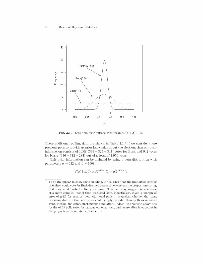
Figure 3.1 displays some beta distributions with different values of α andβ in order to clarify these ideas. All three displayed beta distributions havea mean of .5, but they each have different variances as a result of having αand β parameters of different magnitude. The most-peaked beta distributionhas parameters α = β = 50. The least-peaked distribution is actually flat—uniform—with parameters α = β = 1. As with the binomial distribution, thebeta distribution becomes skewed if α and β are unequal, but the basic ideais the same: the larger the parameters, the more prior information and thenarrower the density.

Returning to the voting example, CNN/USAToday/Gallup had conductedthree previous polls, the results of which could be treated as prior information.

3 Virtually all priors, despite sometimes being called “noninformative,” impartsome information to the posterior distribution. Another way to say this is thatclaiming ignorance is, in fact, providing some information! However, flat priorsgenerally have little weight in affecting posterior inference, and so they are callednoninformative. See Box and Tiao 1973; Gelman et al. 1995; and Lee 1989.


0.0 0.2 0.4 0.6 0.8 1.0

02

46

810

K

Frequency

Beta(1,1)

Beta(5,5)

Beta(50,50)

Fig. 3.1. Three beta distributions with mean α/(α+ β) = .5.

These additional polling data are shown in Table 3.1.4 If we consider theseprevious polls to provide us prior knowledge about the election, then our priorinformation consists of 1,008 (339 + 325 + 344) votes for Bush and 942 votesfor Kerry (346 + 312 + 284) out of a total of 1,950 votes.

This prior information can be included by using a beta distribution withparameters α = 942 and β = 1008:

f(K | α, β) ∝ K942−1(1−K)1008−1.

4 The data appear to show some trending, in the sense that the proportion statingthat they would vote for Bush declined across time, whereas the proportion statingthat they would vote for Kerry increased. This fact may suggest considerationof a more complex model than discussed here. Nonetheless, given a margin oferror of ±4% for each of these additional polls, it is unclear whether the trendis meaningful. In other words, we could simply consider these polls as repeatedsamples from the same, unchanging population. Indeed, the website shows theresults of 22 polls taken by various organizations, and no trending is apparent inthe proportions from late September on.


Table 3.1. CNN/USAToday/Gallup 2004 presidential election polls.

Date n % for Bush ≈ n % for Kerry ≈ n

Oct 17-20 706 48% 339 49% 346Sep 25-28 664 49% 325 47% 312Sep 4-7 661 52% 344 43% 284TOTAL 2,031 1,008 942

Note: Proportions and candidate-specific sample sizes may not add to 100% of totalsample n, because proportions opting for third-party candidates have been excluded.

After combining this prior with the binomial likelihood for the current sample,we obtain the following posterior density for K:

p(K | α, β, x) ∝ K556(1−K)511K941(1−K)1007 = K1497(1−K)1518.

This posterior density is also a beta density, with parameters α = 1498 andβ = 1519, and highlights the important concept of “conjugacy” in Bayesianstatistics. When the prior and likelihood are of such a form that the poste-rior distribution follows the same form as the prior, the prior and likelihoodare said to be conjugate. Historically, conjugacy has been very important toBayesians, because, prior to the development of the methods discussed in thisbook, using conjugate priors/likelihoods with known forms ensured that theposterior would be a known distribution that could be easily evaluated toanswer the scientific question of interest.

Figure 3.2 shows the prior, likelihood, and posterior densities. The likeli-hood function has been normalized as a proper density for K, rather than x.The figure shows that the posterior density is a compromise between the priordistribution and the likelihood (current data). The prior is on the left side ofthe figure; the likelihood is on the right side; and the posterior is between,but closer to the prior. The reason the posterior is closer to the prior is thatthe prior contained more information than the likelihood: There were 1,950previously sampled persons and only 1,067 in the current sample.5

With the posterior density determined, we now can summarize our up-dated knowledge about K, the proportion of voters in Ohio who will vote forKerry, and answer our question of interest: What is the probability that Kerrywould win Ohio? A number of summaries are possible, given that we have aposterior distribution with a known form (a beta density). First, the meanof K is 1498/(1498 + 1519) = .497, and the median is also .497 (found usingthe qbeta function in R). The variance of this beta distribution is .00008283(standard deviation=.0091). If we are willing to assume that this beta distri-bution is approximately normal, then we could construct a 95% interval basedon a normal approximation and conclude that the proportion of Ohio voters

5 This movement of the posterior distribution away from the prior and toward thelikelihood is sometimes called “Bayesian shrinkage” (see Gelman et al. 1995).


0.40 0.45 0.50 0.55 0.60

010

20

30

40

50

60

K

f(K)

Prior (Normalized)

Likelihood

Posterior

Fig. 3.2. Prior, likelihood, and posterior for polling data example: The likelihoodfunction has been normalized as a density for the parameter K.

who would vote for Kerry falls between .479 and .515 (.497±1.96×.0091). Thisinterval is called a “credible interval,” a “posterior probability interval,” or a“probability interval,” and it has a simpler interpretation than the classicalconfidence interval. Using this interval, we can say simply that the proportionK falls in this interval with probability .95.

If, on the other hand, we are not willing to assume that this posteriordensity is approximately normal, we can directly compute a 95% probabilityinterval by selecting the lower and upper values of this beta density thatproduce the desired interval. That is, we can determine the values of this betadensity below which 2.5% of the distribution falls and above which 2.5% ofthe distribution falls. These values are .479 and .514, which are quite close tothose under the normal approximation.

These results suggest that, even with the prior information, the electionmay have been too close to call, given that the interval estimate for K captures.5. However, the substantive question—what is the probability that Kerrywould win—can also be answered within the Bayesian framework. This prob-ability is the probability that Kerry will get more than half of the votes, which


is simply the probability that K > .5. This probability can be directly com-puted from the beta distribution as the integral of this density from .5 to 1(the mass of the curve to the right of .5; see Figure 3.3). The result is .351,which means that Kerry did not have a favorable chance to win Ohio, giventhe complete polling data.

0.40 0.45 0.50 0.55 0.60

010

20

30

40

K

f(K)

p(K>.5)=.351p(K<.5)=.649

Fig. 3.3. Posterior for polling data example: A vertical line at K = .5 is included toshow the area needed to be computed to estimate the probability that Kerry wouldwin Ohio.

In fact, Kerry did not win Ohio; he obtained 48.9% of the votes cast foreither Kerry or Bush. The classical analysis did not yield this conclusion: Itsimply suggested that the results were too close to call. The Bayesian anal-ysis, on the other hand, while recognizing that the election would be close,suggested that there was not a very high probability that Kerry would win.The price that had to be paid for reaching this conclusion, however, was (1)we had to be willing to specify a prior probability for K, and (2) we had tobe willing to treat the parameter of interest as a random, and not a fixed,quantity.


3.3.2 An alternative model for the polling data: A gamma prior/Poisson likelihood approach

In this section, I repeat the analysis from the previous section. However, in-stead of considering the problem as a binomial problem with the proportionparameter p, I consider the problem as a Poisson distribution problem withrate parameter λ. As we discussed in the previous chapter, the Poisson dis-tribution is a distribution for count variables; we can consider an individual’spotential vote for Kerry as a discrete count that takes values of either 0 or 1.From that perspective, the likelihood function for the 1,067 sample membersin the most recent survey prior to the election is:

L(λ|Y ) =1067∏

i=1

λyie−λ

yi!=λ

P

1067

i=1yie−1067λ

∏1067i=1 yi!

,

where yi is the 0 (Bush) or 1 (Kerry) vote of the ith individual.As in the binomial example, we would probably like to include the previ-

ous survey data in our prior distribution. A conjugate prior for the Poissondistribution is a gamma distribution. The pdf of the gamma distribution is asfollows. If x ∼ gamma(α, β), then:

f(x) =βα

Γ (α)xα−1e−βx.

The parameters α and β in the gamma distribution are shape and inverse-scale parameters, respectively. The mean of a gamma distribution is α/β, andthe variance is α/β2. Figure 3.4 shows four different gamma distributions. Asthe plot shows, the distribution is very flexible: Slight changes in the α andβ parameters—which can take any non-negative value—yield highly variableshapes and scales for the density.

For the moment, we will leave α and β unspecified in our voting model sothat we can see how they enter into the posterior distribution. If we combinethis gamma prior with the likelihood function, we obtain:

p(λ | Y ) ∝(

βα

Γ (α)

)

λα−1e−βλ

(

1∏1067

i=1 yi!

)

λP

1067

i=1yie−1067λ.

This expression can be simplified by combining like terms and excluding thearbitrary proportionality constants (the terms in parentheses, which do notinclude λ) to obtain:

p(λ | y) ∝ λP

1067

i=1yi+α−1e−(1067+β)λ.

Given that each yi is either a 0 (vote for Bush) or 1 (vote for Kerry),∑1067

i=1 yi

is simply the count of votes for Kerry in the current sample (=556). Thus,just as in the binomial example, the parameters α and β—at least in this


0 5 10 15 20

0.0

0.2

0.4

0.6

0.8

1.0

x

f(x)

G(1,1)

G(10,1)

G(1,.1)

G(20,2

Fig. 3.4. Some examples of the gamma distribution.

particular model—appear to capture prior “successes” and “failures.” Specif-ically, α is the count of prior “successes,” and β is the total number of priorobservations. The mean of the gamma distribution (α/β) also supports thisconclusion. Thus, as in the beta prior/binomial likelihood example, if we wantto incorporate the data from previous survey into the prior distribution, wecan set α = 942 and β = 942 + 1008 = 1950 to obtain the following posterior:

p(λ | Y ) ∝ λ556+942−1e−(1067+1950)λ = λ1497e−3017λ.

Thus, the posterior density is also a gamma density with parameters α =1498 and β = 3017. Because the gamma density is a known density, we canimmediately compute the posterior mean and standard deviation for λ: λ̄ =.497; σ̂λ = .0128. If we wish to construct a 95% probability/credible intervalfor λ, and we are willing to make a normal approximation given the largesample size, we can construct the interval as .497± 1.96× .0128. This resultgives us an interval estimate of [.472, .522] for λ. On the other hand, if wewish to compute the interval directly using integration of the gamma density(i.e., the cdf for the gamma distribution), we obtain an interval of [.472, .522].


In this case, the normal-theory interval and the analytically derived intervalare the same when rounded to three decimal places.

How does this posterior inference compare with that obtained using thebeta prior/binomial likelihood approach? The means forK in the beta/binomialapproach and for λ in the gamma/Poisson approach are identical. The inter-vals are also quite comparable, but the interval in this latter approach iswider—about 42% wider. If we wish to determine the probability that Kerrywould win Ohio, we simply need to compute p(λ > .5), which equals .390.Thus, under this model, Kerry had a probability of winning of .390, which isstill an unfavorable result, although it is a slightly greater probability thanthe beta/binomial result of .351.

Which model is to be preferred? In this case, the substantive conclusionwe reached was comparable for the two models: Kerry was unlikely to winOhio. So, it does not matter which model we choose. The fact that the twomodels produced comparable results is reassuring, because the conclusion doesnot appear to be very sensitive to choice of model. Ultimately, however, weshould probably place greater emphasis on the beta/binomial model, becausethe Poisson distribution is a distribution for counts, and our data, whichconsisted of dichotomous outcomes, really does not fit the bill. Consider theparameter λ: There is no guarantee with the gamma/Poisson setup that λ willbe less than 1. This lack of limit could certainly be problematic if we had lessdata, or if the underlying proportion favoring Kerry were closer to 1. In sucha case, the upper bound on the interval for λ may have exceeded 1, and ourresults would therefore be suspect. In this particular case, however, we hadenough data and prior information that ultimately made the interval widthvery narrow, and so the bounding problem was not an issue. Nonetheless, thebeta/binomial setup is a more natural model for the voting data.

3.4 A normal prior–normal likelihood example with σ2

known

The normal distribution is one of the most common distributions used instatistics by social scientists, in part because many social phenomena in factfollow a normal distribution. Thus, it is not uncommon for a social scientistto use a normal distribution as the basis for a likelihood function for a set ofdata. Here, I develop a normal distribution problem, but for the sake of keepingthis example general for use in later chapters, I used a contrived scenario andkeep the mathematics fairly general. The purpose at this point is simply toillustrate a Bayesian approach with a multivariate posterior distribution.6

6 The normal distribution involves two parameters: the mean (µ) and variance (σ2).When considered as a density for x, it is univariate, but when a normal likelihoodand some prior for the parameters are combined, the result is a joint posteriordistribution for µ and σ2, which makes the posterior a multivariate density.

3.4 A normal prior–normal likelihood example with σ2 known 63

Suppose that we have a class of 30 students who have recently taken amidterm exam, and the mean grade was x̄ = 75 with a standard deviation ofσ = 10. Note that for now we have assumed that the variance is known, hence,the use of σ rather than s. We have taught the course repeatedly, semesterafter semester, and past test means have given us an overall mean µ of 70, butthe class means have varied from class to class, giving us a standard deviationfor the class means of τ = 5. That is, τ reflects how much our class means havevaried and does not directly reflect the variability of individual test scores.We will discuss this more in depth momentarily.

Our goal is ultimately to update our knowledge of µ, the unobservablepopulation mean test score with the new test grade data. In other words, wewish to find f(µ|x). Bayes’ Theorem tells us that:

f(µ|X) ∝ f(X|µ)f(µ),

where f(X|µ) is the likelihood function for the current data, and f(µ) is theprior for the test mean. (At the moment, I am omitting σ2 from the notation).If we assume the current test scores are normally distributed with a meanequal to µ and variance σ2, then our likelihood function for X is:

f(X|µ) ∝ L(µ|X) =n∏

i=1

1√2πσ2

exp

{

− (xi − µ)2

2σ2

}

.

Furthermore, our previous test results have provided us with an overall meanof 70, but we are uncertain about µ’s actual value, given that class meansvary semester by semester (giving us τ = 5). So our prior distribution for µis:

f(µ) =1√

2πτ2exp

{

− (µ−M)2

2τ2

}

,

where in this expression, µ is the random variable, with M as the prior mean(=70), and τ2 (=25) reflects the variation of µ around M .

Our posterior is the product of the likelihood and prior, which gives us:

f(µ|X) ∝ 1√τ2σ2

exp

{−(µ−M)2

2τ2+−∑n

i=1(xi − µ)2

2σ2

}

.

This posterior can be reexpressed as a normal distribution for µ, but it takessome algebra in order to see this. First, since the terms outside the exponentialare simply normalizing constants with respect to µ, we can drop them andwork with the terms inside the exponential function. Second, let’s expandthe quadratic components and the summations. For the sake of simplicty, Itemporarily drop the exponential function in this expression:

(−1/2)

[

µ2 − 2µM +M2

τ2+

∑

x2 − 2nx̄µ+ nµ2

σ2

]

.


Using this expression, any term that does not include µ can be viewed asa proportionality constant, can be factored out of the exponent, and can bedropped (recall that ea+b = eaeb). After obtaining common denominators forthe remaining terms by cross-multiplying by each of the individual denomi-nators and dropping proportionality constants, we are left with:

(−1/2)

[

σ2µ2 − 2σ2µM − 2τ2nx̄µ+ τ2nµ2

σ2τ2

]

.

From here, we need to combine terms involving µ2 and those involving µ:

(−1/2)

[

(nτ2 + σ2)µ2 − 2(σ2M + τ2nx̄)µ

σ2τ2

]

.

Dividing the numerator and denominator of this fraction by the (nτ2 + σ2)in front of µ2 yields:

(−1/2)

µ2 − 2µ (σ2M+nτ2x̄)(nτ2+σ2)

σ2τ2

(nτ2+σ2)

.

Finally, all we need to do is to complete the square in µ and discard anyremaining constants to obtain:

(−1/2)

(

µ− (σ2M+nτ2x̄)(nτ2+σ2)

)2

σ2τ2

(nτ2+σ2)

.

This result shows that our updated µ is normally distributed with mean(σ2M + τ2nx̄)/(nτ2 + σ2) and variance (σ2τ2)/(nτ2 + σ2). Notice how theposterior mean is a weighted combination of the prior mean and the samplemean. The prior mean is multiplied by the known variance of test scores in thesample, σ2, whereas the sample mean x̄ is multiplied by n and by the priorvariance τ2. This shows first that the sample mean will tend to have moreweight than the prior mean (because of the n multiple), but also that theprior and sample variances affect the weighting of the means. If the samplevariance is large, then the prior mean has considerable weight in the poste-rior; if the prior variance is large, the sample mean has considerable weight inthe posterior. If the two quantities are equal (σ2 = τ2), then the calculationreduces to (M +nx̄)/(n+1), which means that the prior mean will only havea weight of 1/(n+ 1) in the posterior.

In this particular example, our posterior mean would be:

(100× 70) + (25× 30× 75)/(30× 25 + 100) = 74.4.

Thus, our result is clearly more heavily influenced by the sample data thanby the prior. One thing that must be kept in mind but is easily forgotten isthat our updated variance parameter (which is 20—the standard deviation is


therefore 4.47) reflects our uncertainty about µ. This estimate is smaller thanboth the prior variance and the sample variance, and it is much closer to τ2

than to σ2. Why? Again, this quantity reflects how much µ varies (or, putanother way, how much uncertainty we have in knowing M , the true valueof µ) and not how much we know about any particular sample. Thus, thefact that our sample standard deviation was 10 does not play a large role inchanging our minds about uncertainty in µ, especially given that the samplemean was not that different from the prior mean. In other words, our samplemean is sufficiently close to our prior mean µ so that we are unconvinced thatthe variance of µ around M should be larger than it was. Indeed, the dataconvince us that our prior variance should actually be smaller, because thecurrent sample mean is well within the range around M implied by our priorvalue for τ .

3.4.1 Extending the normal distribution example

The natural extension of the previous example in which the variance σ2 wasconsidered known is to consider the more realistic case in which the variance isnot known. Recall that, ultimately in the previous example, we were interestedin the quantity µ—the overall mean test score. Previous data had given us anestimate of µ, but we were still uncertain about its value, and thus, we usedτ to represent our uncertainty in µ. We considered σ2 to be a known quantity(10). In reality, we typically do not know σ2 any more than we know µ, andthus we have two quantities of interest that we should be updating with newinformation. A full probability model for µ and σ2 would look like:

f(µ, σ2|x) ∝ f(x|µ, σ2)f(µ, σ2).

This model is similar to the one in the example above, but we have nowexplicitly noted that σ2 is also an unknown quantity, by including it in theprior distribution. Therefore, we now need to specify a joint prior for both µand σ2, and not just a prior for µ. If we assume µ and σ2 are independent—and this is a reasonable assumption as we mentioned in the previous chapter;there’s no reason the two parameters need be related—then we can considerp(µ, σ2) = p(µ)p(σ2) and establish separate priors for each.

In the example above, we established the prior for µ to be µ ∼ N(M, τ2),where M was the prior mean (70) and τ2 was the measure of uncertaintywe had in µ. We did not, however, specify a prior for σ2, but we used σ2 toupdate our knowledge of τ .7

How do we specify a prior distribution for µ and σ2 in a more general case?Unlike in the previous example, we often do not have prior information aboutthese parameters, and so we often wish to develop noninformative priors for

7 Recall from the CLT that x̄ ∼ N(µ, σ2/n); thus σ2 and τ2 are related: σ2/nshould be an estimate for τ2, and so treating σ2 as fixed yields an updated τ2

that depends heavily on the new sample data.


them. There are several ways to do this in the normal distribution problem,but two of the most common approaches lead to the same prior. One approachis to assign a uniform prior over the real line for µ and the same uniform priorfor log(σ2). We assign a uniform prior on log(σ2) because σ2 is a nonega-tive quantity, and the transformation to log(σ2) stretches this new parameteracross the real line. If we transform the uniform prior on log(σ2) into a densityfor σ2, we obtain p(σ2) ∝ 1/σ2.8 Thus, our joint prior is: p(µ, σ2) ∝ 1/σ2.

A second way to obtain this prior is to give µ and σ2 proper prior distribu-tions (not uniform over the real line, which is improper). If we continue withthe assumption that µ ∼ N(M, τ2), we can choose values of M and τ2 thatyield a flat distribution. For example, if we let µ ∼ N(0, 10000), we have avery flat prior for µ. We can also choose a relatively noninformative prior forσ2 by first noting that variance parameters follow an inverse gamma distri-bution (see the next section) and then choosing values for the inverse gammadistribution that produce a noninformative prior. If σ2 ∼ IG(a, b), the pdfappears as:

f(σ2|a, b) ∝ (σ2)−(a+1)e−β/(σ2).

In the limit, if we let the parameters a and b approach 0, a noninformativeprior is obtained as 1/σ2. Strictly speaking, however, if a and b are 0, thedistribution is improper, but we can let both parameters approach 0. We canthen use this as our prior for σ2 (that is, σ2 ∼ IG(0, 0); p(σ2) ∝ 1/σ2). Thereare other ways to arrive at this choice for the prior distribution for µ and σ,but I will not address them here (see Gelman et al. 1995).

The resulting posterior for µ and σ2, if we assume a joint prior of 1/σ2 forthese parameters, is:

f(µ, σ2|X) ∝ 1

σ2

n∏

i=1

1√2πσ2

exp

{

− (xi − µ)2

2σ2

}

. (3.4)

Unlike in the previous example, however, this is a joint posterior densityfor two parameters rather than one. Yet we can determine the conditional

posterior distributions for both parameters, using the rule discussed in theprevious chapter that, generally, f(x|y) ∝ f(x, y).

Determining the form for the posterior density for µ follows the same logicas in the previous section. First, we carry out the product over all observations.Next, we expand the quadratic, eliminate terms that are constant with respectto µ and rearrange the terms with the µ2 term first. Doing so yields:

8 This transformation of variables involves a Jacobian, as discussed in the previouschapter. Let m = log(σ2), and let p(m) ∝ constant. Then p(σ2) ∝ constant× J ,where J is the Jacobian of the transformation from m to σ2. The Jacobian is thendm/dσ2 = 1/σ2. See DeGroot (1986) for a fuller exposition of this process, andsee any introductory calculus book for a general discussion of transformations ofvariables. See Gelman et al. 1995 for further discussion of this prior.


f(µ|X,σ2) ∝ exp

{

−nµ2 − 2nx̄µ

2σ2

}

.

Next, to isolate µ2, we can divide the numerator and denominator by n.Finally, we can complete the square in µ to find:

f(µ|X,σ2) ∝ exp

{

− (µ− x̄)2

2σ2/n

}

.

This result shows us that the conditional distribution for µ|X,σ2 ∼ N(x̄, σ2

n ),which should look familiar. That is, this is a similar result to what the CentralLimit Theorem in classical statistics claims regarding the sampling distribu-tion for x̄.

What about the posterior distribution for σ2? There are at least two waysto approach this derivation. First, we could consider the conditional distribu-tion for σ2|µ,X. If we take this approach, then we again begin with the fullposterior density, but we now must consider all terms that involve σ2. If wecarry out the multiplication in the posterior density and combine like terms,we obtain:

f(µ, σ2) ∝ 1

(σ2)n/2+1exp

{

−∑

(xi − µ)2

2σ2

}

.

Referring back to the above description of the inverse gamma distribution, itis clear that, if µ is considered fixed, the conditional posterior density for σ2

is inverse gamma with parameters a = n/2 and b =∑

(xi − µ)2/2.A second way to approach this problem is to consider that the joint pos-

terior density for µ and σ2 can be factored using the conditional probabilityrule as:

f(µ, σ2|X) = f(µ|σ2, X)f(σ2|X).

The first term on the right-hand side we have already considered in the pre-vious example with σ2 considered to be a known, fixed quantity. The latterterm, however, is the marginal posterior density for σ2. Technically, an exactexpression for it can be found by integrating the joint posterior density overµ (i.e.,

∫

f(µ, σ2)dµ.) (see Gelman et al. 1995). Alternatively, we can find anexpression proportional to it by factoring Equation 3.4. We know that thedistribution for µ|σ2, X is proportional to a normal density with mean x̄ andvariance σ2/n. Thus, if we factor this term out of the posterior, what is leftis proportional to the marginal density for σ2.

In order to factor the posterior, first, expand the quadratic again to obtain:

1

(σ2)n/2+1exp

{

−∑

x2i − 2nx̄µ+ nµ2

2σ2

}

.

Next, rearrange terms to put µ2 first, and divide the numerator and denomi-nator by n. Once again, complete the square to obtain:


1

(σ2)n/2+1exp

{

− (µ− x̄)2 +∑

x2i /n− x̄2

2σ2/n

}

.

We can now separate the two parts of the exponential to obtain:

1

σexp

{

− (µ− x̄)2

2σ2/n

}

× 1

(σ2)n/2exp

{∑

x2i − nx̄2

2σ2

}

.

The first term is the conditional posterior for µ. The latter term is proportionalto the marginal posterior density for σ2. The numerator in the exponential isthe numerator for the computational version of the sample variance,

∑

(xi −x̄)2, and so, the result is recognizable as an inverse gamma distribution withparameters a = (n− 1)/2 and b = (n− 1)var(x)/2.

3.5 Some useful prior distributions

Thus far, we have discussed the use of a beta prior for proportion parameterp combined with a binomial likelihood function, a gamma prior for a Poissonrate parameter λ, a normal prior for a mean parameter combined with anormal likelihood function for the case in which the variance parameter σ2

was assumed to be known, and a reference prior of 1/σ2—a special case of aninverse gamma distribution—for a normal likelihood function for the case inwhich neither µ nor σ2 were assumed to be known. In this section, I discuss afew additional distributions that are commonly used as priors for parametersin social science models. These distributions are commonly used as priors,because they are conjugate for certain sampling densities/likelihood functions.Specifically, I discuss the Dirichlet, the inverse gamma (in some more depth),and the Wishart and inverse Wishart distributions.

One thing that must be kept in mind when considering distributions aspriors and/or sampling densities is what symbols in the density are parameters

versus what symbols are the random variables. For example, take the binomialdistribution discussed in Chapter 2. In the binomial mass function, the ran-dom variable is represented by x, whereas the parameter is represented byp. However, in the beta distribution, the random variable is represented byp and the parameters are α and β. From a Bayesian perspective, parametersare random variables or at least can be treated as such. Thus, what is im-portant to realize is that we may need to change notation in the pdf so thatwe maintain the appropriate notation for representing the prior distributionfor the parameter(s). For example, if we used θ to represent the parameter pin the binomial likelihood function, while p is used as the random variable inthe beta distribution, the two distributions, when multiplied together, wouldcontain p, θ, and x, and it would be unclear how θ and p were related. In fact,in the beta-binomial setup, θ = p, but we need to make sure our notation isclear so that that can be immediately seen.

3.5 Some useful prior distributions 69

3.5.1 The Dirichlet distribution

Just as the multinomial distribution is a multivariate extension of the bi-nomial distribution, the Dirichlet distribution is a multivariate generaliza-tion of the beta distribution. If X is a k-dimensional vector and X ∼Dirichlet(α1, α2, . . . , αk), then:

f(X) =Γ (α1 + . . .+ αk)

Γ (α1) . . . Γ (αk)xα1−1

1 . . . xαk−1k .

Just as the beta distribution is a conjugate prior for the binomial distribution,the Dirichlet is a conjugate prior for the multinomial distribution. We can seethis result clearly, if we combine a Dirichlet distribution as a prior with amultinomial distribution likelihood:

f(p1 . . . pk|X) ∝ f(X|p1 . . . pk)f(p1 . . . pk)

∝ Multinomial(X|p1 . . . pk)Dirichlet(p1 . . . pk|α1 . . . αk)

∝ Dirichlet(p1 . . . pk|α1 + x1, α2 + x2, . . . , αk + xk)

∝ pα1+x1−11 pα2+x2−1

2 . . . pαk+xk−1k .

Notice how here, as we discussed at the beginning of the section, the vector Xin the original specification of the Dirichlet pdf has been changed to a vectorp. In this specification, p is the random variable in the Dirichlet distribution,whereas α1 . . . αk are the parameters representing prior counts of outcomes ineach of the k possible outcome categories.

Also observe how the resulting Dirichlet posterior distribution looks justlike the resulting beta posterior distribution, only with more possible out-comes.

3.5.2 The inverse gamma distribution

We have already discussed the gamma distribution in the Poisson/gammaexample, and we have briefly discussed the inverse gamma distribution. If1/x ∼ gamma(α, β), then x ∼ IG(α, β). The density function for the inversegamma distribution is:

f(x) =βα

Γ (α)x−(α+1)e−β/x,

with x > 0. Just as in the gamma distribution, the parameters α and β affectthe shape and scale of the curve (respectively), and both must be greater than0 to make the density proper.

As discussed earlier, the inverse gamma distribution is used as a conju-gate prior for the variance in a normal model. If the normal distribution isparameterized with a precision parameter rather than with a variance param-eter, where the precision parameter is simply the inverse of the variance, the


gamma distribution is appropriate as a conjugate prior distribution for theprecision parameter. In a normal model, if an inverse gamma distribution isused as the prior for the variance, the marginal distribution for the mean is at distribution.

The gamma and inverse gamma distributions are general distributions;other distributions arise by fixing the parameters to specific values. For ex-ample, if α is set to 1, the exponential distribution results:

f(x) = (1/β)e−x/β ,

or, more commonly f(x) = βe−βx, where β is an inverse scale parameter.Under this parameterization, βinverse scale = 1/βscale.

If α is set to v/2, where v is the degrees of freedom, and β is set to 1/2, thechi-square distribution results. Setting the parameters equal to the same valuein the inverse-gamma distribution yields an inverse-chi-square distribution.

3.5.3 Wishart and inverse Wishart distributions

The Wishart and inverse Wishart distributions are complex in appearance;they are multivariate generalizations of the gamma and inverse gamma dis-tributions, respectively. Thus, just as the inverse gamma is a conjugate priordensity for the variance in a univariate normal model, the inverse Wishartis a conjugate prior density for the variance-covariance matrix in a multi-variate normal model. With an inverse Wishart distribution for the variance-covariance matrix in a multivariate normal model, the marginal distributionfor the mean vector is multivariate t.

If X ∼Wishart(S), where S is a scale matrix of dimension d, then

f(X) ∝| X |(v−d−1)/2 exp

{

−1

2tr(S−1X)

}

,

where v is the degrees of freedom.If X ∼ inverse Wishart(S−1), then:

f(X) ∝| X |−(v+d+1)/2 exp

{

−1

2tr(SX−1)

}

.

The assumption for both the Wishart and inverse Wishart distributions isthat X and S are both positive definite; that is, zTXz > 0 and zTSz > 0 forany non-zero vector z of length d.

3.6 Criticism against Bayesian statistics

As we have seen in the examples, the development of a Bayesian model re-quires the inclusion of a prior distribution for the parameters in the model.The notion of using prior research or other information to inform a current

3.6 Criticism against Bayesian statistics 71

analysis and to produce an updated prior for subsequent use seems quite rea-sonable, if not very appropriate, for the advancement of research toward amore refined knowledge of the parameters that govern social processes. How-ever, the Bayesian approach to updating knowledge of parameters has beencriticized on philosophical grounds for more than a century, providing onereason its adoption has been relatively limited in mainstream social scienceresearch.

What is in philosophical dispute between Bayesians and classical statisti-cians includes: (1) whether data and hypotheses (which are simply statementsabout parameters of distributions9) can hold the same status as random vari-ables, and (2) whether the use of a prior probability injects too much subjec-tivity into the modeling process.

The first standard argument presented against the Bayesian approach isthat, because parameters are fixed, it is unreasonable to place a probabilitydistribution on them (they simply are what they are). More formally, pa-rameters and data cannot share the same sample space. However, recall thatthe Bayesian perspective on probability is that probability is a subjective ap-proach to uncertainty. Whether a parameter is indeed fixed, to a Bayesian, isirrelevant, because we are still uncertain about its true value. Thus, impos-ing a probability distribution over a parameter space is reasonable, becauseit provides a method to reflect our uncertainty about the parameter’s truevalue.

Bayesians argue that doing so has some significant advantages. First, aswe have seen, Bayesian interval estimates have a clearer and more direct inter-pretation than classical confidence intervals. That is, we can directly concludethat a parameter falls in some interval with some probability. This is a com-mon but incorrect interpretation of classical confidence intervals, which simplyreflect the probability of obtaining an interval estimate that contains the pa-rameter of interest under repeated sampling. Second, the Bayesian approachcan naturally incorporate the findings of previous research with the prior,whereas the classical approach to statistics really has no coherent means ofusing previous results in current analyses beyond assisting with the specifica-tion of a hypothesis. That is, the Bayesian approach formalizes the process ofhypothesis construction by incorporating it as part of the model. Third, theBayesian approach more easily allows more detailed summaries concerningparameters. Instead of simply obtaining a maximum likelihood estimate andstandard error, we have an entire distribution that can be summarized usingvarious measures (e.g., mean, median, mode, and interquartile range).

9 An alternative representation of Bayes’ Theorem is p(Hypothesis | data) ∝p(data | Hypothesis) × p(Hypothesis), which shows that, from a Bayesian per-spective, we can place a probability (distribution) on a scientific hypothesis. SeeJeffreys 1961 for a detailed discussion of the theory of “inverse probability,” whichdescribes the Bayesian approach in these terms.


The second general argument that has been advanced against Bayesiananalysis is that incorporating a prior injects too much subjectivity into statis-tical modeling. The Bayesian response to this argument is multifaceted. First,all statistics is subjective. The choice of sampling density (likelihood) to usein a specific project is a subjective determination. For example, when facedwith an ordinal outcome, some choose to use a normal likelihood function,leading to the ordinary least squares (OLS) regression model. Others choose abinomial likelihood with a link function, leading to an ordinal logit or probitregression model. These are subjective choices.

Second, the choice of cut-point (α) at which to declare a result “statisti-cally significant” in a classical sense is a purely subjective determination. Also,similarly, the decision to declare a statistically significant result substantivelymeaningful is a subjective decision.

A third response to the subjectivity criticism is that priors tend to beoverwhelmed by data, especially in social science research. The prior distribu-tion generally contributes to the posterior once, whereas data enter into thelikelihood function multiple times. As n → ∞, the prior’s influence on theposterior often becomes negligible.

Fourth, priors can be quite noninformative, obviating the need for largequantities of data to “outweigh” them. In other words, a prior can be madeto contribute little information to the posterior. That is, given that the pos-terior density is simply a weighted likelihood function, where the weightingis imposed by the prior, we can simply choose a prior distribution for theparameters that assigns approximately equal weight to all possible values ofthe parameters. The simplest noninformative prior that is often used is thus auniform prior. Use of this prior yields a posterior density that is proportionalto the likelihood function. In that case, the mode of the likelihood function(the maximum likelihood estimate) is the same as the Bayesian maximum a

posteriori (MAP) estimate, and the substantive conclusions reached by bothapproaches may be similar, only differing in interpretation.

In defense of the classical criticism, although uniform densities for param-eters are often used as priors, transformation from one parameterization ofa parameter to another may yield an informative prior. However, alternativeapproaches have been developed for generating noninformative priors, includ-ing the development of Jeffreys priors and other priors. These noninformativepriors tend to be based on the information matrix and are invariant under pa-rameter transformation. An in-depth discussion of such priors is beyond thescope of this book, given the goal of a general introduction to estimation. Formore details, see Gelman et al. (1995) or see Gill (2002) for a more in-depthdiscussion of the history of the use and construction of noninformative priors.

A fourth response is that the influence of priors can be evaluated aftermodeling the data to determine whether posterior inference is reasonable. Ul-timately, the results of any statistical analysis, whether Bayesian or classical,must be subjectively evaluated to determine whether they are reasonable, andso, the use of informative priors cannot introduce any more subjectivity than

3.7 Conclusions 73

could be included via other means in any analysis. Another response alongthese lines is that we can use priors to our advantage to examine how pow-erful the data are at invalidating the prior. For example, we may establisha conservative prior for a regression coefficient that claims that the a priori

probability for a regression coefficient is heavily concentrated around 0 (i.e.,the covariate has no effect on the outcome). We can then examine the strengthof the data in rejecting this prior, providing a conservative test of a covariate’seffect.

In general, the historical criticisms of Bayesian statistics are philosophicalin nature and cannot be conclusively adjudicated. Instead, the rise in theuse of Bayesian statistics over the last few decades has largely occurred forpragmatic reasons, including (1) that many contemporary research questionsreadily lend themselves to a Bayesian approach, and (2) that the developmentof sampling methods used to estimate model parameters has increased theirease of use. The remaining chapters attempt to demonstrate these points.

3.7 Conclusions

In this chapter, we have developed the basics of the Bayesian approach tostatistical inference. First, we derived Bayes’ Theorem from the probabilityrules developed in the previous chapter, and we applied Bayes’ Theorem toproblems requiring point estimates for probabilities. We then extended theBayesian approach to handle prior distributions for parameters rather thansimply point estimates for prior probabilties. The result was that our posteriorprobability became a distribution, rather than a point estimate. Next, we dis-cussed how to summarize posterior probability distributions, and we demon-strated how to do so using several common examples. Finally, we discussedsome common criticisms of the Bayesian approach that have been advancedover the last century, and we reviewed some common Bayesian responses tothem. Although the material presented in this chapter is sufficient for gaininga basic understanding of the Bayesian approach to statistics, I recommendseveral additional sources for more in-depth coverage. I recommend Lee 1989for an extremely thorough but accessible exposition of the Bayesian paradigm,and I recommend Box and Tiao (1973) for a more advanced exposition.

In the next chapter, we will continue exploring the Bayesian approachto posterior summarization and inference, but we will ultimately focus onmultivariate posterior distributions—the most common type of posterior dis-tribution found in social science research—where the multivariate posteriordistribution may not be as easy to summarize directly as the univariate pos-terior densities shown in this chapter.


3.8 Exercises

1. In your own words, state what Bayes’ Theorem for point probabilities ac-tually does. For example, refer to Chapter 2 where I defined conditionalprobability, and use the same sort of discussion to describe how the the-orem works.

2. The pregnancy example was completely contrived. In fact, most pregnancytests today do not have such high rates of false positives. The “accuracyrate” is usually determined by computing the percent of correct answersthe test gives; that is, the combined percent of positive results for positivecases and negative results for negative cases (versus false positives andfalse negatives). Recompute the posterior probability for being pregnantbased on an accuracy rate of 90% defined in this manner. Assume thatfalse positives and false negatives occur equally frequently under this 90%rate. What changes in the calculation?

3. Determine the posterior probability that a 30-year-old male has prostatecancer, given (1) a positive PSA test result; (2) a 90% accuracy rate (asdefined in the pregnancy example), coupled with a 90% false positive rate;and (3) a prior probability of .00001 for a 30-year-old male having prostatecancer. Based on the result, why might a physician consider not testing a30-year-old male using the PSA test?

4. Find and plot the posterior distribution for a binomial likelihood withx = 5 successes out of n = 10 trials using at least three different beta priordistributions. Does the prior make a large difference in the outcome—when?

5. Find and plot the posterior distribution for a normal distribution likeli-hood with a sample mean x̄ = 100 and variance var(x) = 144 (assumen = 169) using at least three different normal priors for the mean. Whendoes the prior make the largest difference in the outcome—when the priormean varies substantially from the sample mean, or when the prior vari-ance is small or large?

6. Reconsider the pregnancy example from the beginning of the chapter. Ishowed the posterior probabilities for the second through the tenth sub-sequent tests. Reproduce these results, using the posterior obtained from

the kth test as the prior for the (k + 1)st test. Next, assume the originalprior (p = .15) and assume the 10 tests were taken simultaneously andall yielded a positive result. What is the posterior probability for preg-nancy? Finally, reconduct the pregnancy example with the 10 positivetests treated simultaneously as the current data, and use a beta priordistribution. Interpret the results.

7. In the 2004 U.S. presidential election, surveys throughout the fall con-stantly reversed the projected victor. As each survey was conducted, wouldit have been appropriate to incorporate the results of previous surveys aspriors and treat the current survey as new data to update the prior ina Bayesian fashion? If so, do you think a more consistent picture of the

3.8 Exercises 75

winner would have emerged before the election? If a Bayesian approachwould not have been appropriate, why not?

8. Give two simple examples showing a case in which a prior distributionwould not be overwhelmed by data, regardless of the sample size.

9. Show how the multinomial likelihood and Dirichlet prior are simply amultivariate generalization of the binomial likelihood and beta prior.

10. Show how the Wishart distribution reduces to the gamma distributionwhen the number of dimensions of the random variable is 1.

11. I said throughout the chapter that the inverse gamma distribution was theappropriate distribution for a variance parameter. It could be said thatvariance parameter could be considered to be distributed as an inversechi-square random variable. Both of these statements are true. How?

12. Why can a prior distribution that equals a constant be considered pro-portional to a uniform distribution?

3 Basics of Bayesian Statistics - Carnegie Mellon Universitybrian/463-663/week09/Chapter 03.pdf ·...

Documents

Transcript of 3 Basics of Bayesian Statistics - Carnegie Mellon Universitybrian/463-663/week09/Chapter 03.pdf ·...