312-2012: Handling Missing Data by Maximum Likelihood€¦ · 1 Paper 312-2012 Handling Missing...

1

Paper 312-2012

Handling Missing Data by Maximum Likelihood Paul D. Allison, Statistical Horizons, Haverford, PA, USA

ABSTRACT

Multiple imputation is rapidly becoming a popular method for handling missing data, especially with easy-to-use software like PROC MI. In this paper, however, I argue that maximum likelihood is usually better than multiple imputation for several important reasons. I then demonstrate how maximum likelihood for missing data can readily be implemented with the following SAS® procedures: MI, MIXED, GLIMMIX, CALIS and QLIM.

INTRODUCTION

Perhaps the most universal dilemma in statistics is what to do about missing data. Virtually every data set of at least moderate size has some missing data, usually enough to cause serious concern about what methods should be used. The good news is that the last twenty five years have seen a revolution in methods for handling missing data. The new methods have much better statistical properties than traditional methods, while at the same time relying on weaker assumptions.

The bad news is that these superior methods have not been widely adopted by practicing researchers. The most likely reason is ignorance. Many researchers have barely even heard of modern methods for handling missing data. And if they have heard of them, they have little idea how to go about implementing them. The other likely reason is difficulty. Modern methods can take considerably more time and effort, especially with regard to start-up costs. Nevertheless, with the development of better software, these methods are getting easier to use every year.

There are two major approaches to missing data that have good statistical properties: maximum likelihood (ML) and multiple imputation (MI). Multiple imputation is currently a good deal more popular than maximum likelihood. But in this paper, I argue that maximum likelihood is generally preferable to multiple imputation, at least in those situations where appropriate software is available. And many SAS users are not fully aware of the available procedures for using maximum likelihood to handle missing data.

In the next section, we’ll examine some assumptions that are commonly used to justify methods for handling missing data. In the subsequent section, we’ll review the basic principles of maximum likelihood and multiple imputation. After I present my arguments for the superiority of maximum likelihood, we’ll see how to use several different SAS procedures to get maximum likelihood estimates when data are missing.

ASSUMPTIONS

To make any headway at all in handling missing data, we have to make some assumptions about how missingness on any particular variable is related to other variables. A common but very strong assumption is that the data are missing completely at random (MCAR). Suppose that only one variable Y has missing data, and that another set of variables, represented by the vector X, is always observed. The data are missing completely at random (MCAR) if the probability that Y is missing does not depend on X or on Y itself (Rubin 1976). To represent this formally, let R be a “response” indicator having a value of 1 if Y is missing and 0 if Y is observed. MCAR means that

)1Pr(),|1Pr( === RYXR

If Y is a measure of delinquency and X is years of schooling, MCAR would mean that the probability that data are missing on delinquency is unrelated to either delinquency or schooling. Many traditional missing data techniques are valid only if the MCAR assumption holds.

A considerably weaker (but still strong) assumption is that data are missing at random (MAR). Again, this is most easily defined in the case where only a single variable Y has missing data, and another set of variables X has no missing data. We say that data on Y are missing at random if the probability that Y is missing does not depend on Y, once we control for X. Formally, we have

)|1Pr(),|1Pr( XRYXR ===

where, again, R is the response indicator. Thus, MAR allows for missingness on Y to depend on other variables that are observed. It just cannot depend on Y itself (after adjusting for the observed variables).

Continuing our example, if Y is a measure of delinquency and X is years of schooling, the MAR assumption would be satisfied if the probability that delinquency is missing depends on years of schooling, but within each level of schooling, the probability of missing delinquency does not depend on delinquency.

Statistics and Data AnalysisSAS Global Forum 2012

2

In essence, MAR allows missingness to depend on things that are observed, but not on things that are not observed. Clearly, if the data are missing completely at random, they are also missing at random.

It is straightforward to test whether the data are missing completely at random. For example, one could compare men and women to test whether they differ in the proportion of cases with missing data on income. Any such difference would be a violation of MCAR. However, it is impossible to test whether the data are missing at random, but not completely at random. For obvious reasons, one cannot tell whether delinquent children are more likely than nondelinquent children to have missing data on delinquency.

What if the data are not missing at random (NMAR)? What if, indeed, delinquent children are less likely to report their level of delinquency, even after controlling for other observed variables? If the data are truly NMAR, then the missing data mechanism must be modeled as part of the estimation process in order to produce unbiased parameter estimates. That means that, if there is missing data on Y, one must specify how the probability that Y is missing depends on Y and on other variables. This is not straightforward because there are an infinite number of different models that one could specify. Nothing in the data will indicate which of these models is correct. And, unfortunately, results could be highly sensitive to the choice of model. A good deal of research has been devoted to the problem of data that are not missing at random, and some progress has been made. Unfortunately, the available methods are rather complex, even for very simple situations.

For these reasons, most commercial software for handling missing data, either by maximum likelihood or multiple imputation, is based on the assumption that the data are missing at random. But near the end of this paper, we’ll look at a SAS procedure that can do ML estimation for one important case of data that are not missing at random.

MULTIPLE IMPUTATION

Although this paper is primarily about maximum likelihood, we first need to review multiple imputation in order to understand its limitations. The three basic steps to multiple imputation are:

1. Introduce random variation into the process of imputing missing values, and generate several data sets, each with slightly different imputed values.

2. Perform an analysis on each of the data sets.

3. Combine the results into a single set of parameter estimates, standard errors, and test statistics.

If the assumptions are met, and if these three steps are done correctly, multiple imputation produces estimates that have nearly optimal statistical properties. They are consistent (and, hence, approximately unbiased in large samples), asymptotically efficient (almost), and asymptotically normal.

The first step in multiple imputation is by far the most complicated, and there are many different ways to do it. One popular method uses linear regression imputation. Suppose a data set has three variables, X, Y, and Z. Suppose X and Y are fully observed, but Z has missing data for 20% of the cases. To impute the missing values for Z, a regression of Z on X and Y for the cases with no missing data yields the imputation equation

YbXbbZ 210ˆ ++=

Conventional imputation would simply plug in values of X and Y for the cases with missing data and calculate predicted values of Z. But those imputed values have too small a variance, which will typically lead to bias in many other parameter estimates. To correct this problem, we instead use the imputation equation

sEYbXbbZ +++= 210ˆ ,

where E is a random draw from a standard normal distribution (with a mean of 0 and a standard deviation of 1) and s is the estimated standard deviation of the error term in the regression (the root mean squared error). Adding this random draw raises the variance of the imputed values to approximately what it should be and, hence, avoids the biases that usually occur with conventional imputation.

If parameter bias were the only issue, imputation of a single data set with random draws would be sufficient. Standard error estimates would still be too low, however, because conventional software cannot take account of the fact that some data are imputed. Moreover, the resulting parameter estimates would not be fully efficient (in the statistical sense), because the added random variation introduces additional sampling variability.

The solution is to produce several data sets, each with different imputed values based on different random draws of E. The desired model is estimated on each data set, and the parameter estimates are simply averaged across the multiple runs. This yields much more stable parameter estimates that approach full efficiency.


3

With multiple data sets we can also solve the standard error problem by calculating the variance of each parameter estimate across the several data sets. This “between” variance is an estimate of the additional sampling variability produced by the imputation process. The “within” variance is the mean of the squared standard errors from the separate analyses of the several data sets. The standard error adjusted for imputation is the square root of the sum of the within and between variances (applying a small correction factor to the latter). The formula (Rubin 1987) is:

==

−

−

++

M

kk

M

kk aa

MMs

M 1

2

1

2 )(1

1111

In this formula, M is the number of data sets, sk is the standard error in the kth data set, ak is the parameter estimate in the kth data set, and a is the mean of the parameter estimates. The factor (1+1/M) corrects for the fact that the number of data sets is finite.

How many data sets are needed? With moderate amounts of missing data, five are usually enough to produce parameter estimates that are more than 90% efficient. More data sets may be needed for good estimates of standard errors and associated statistics, however, especially when the fraction of missing data is large.

THE BAYESIAN APPROACH TO MULTIPLE IMPUTATION

The method just described for multiple imputation is pretty good, but it still produces standard errors that are a bit too low, because it does not account for the fact that the parameters in the imputation equation (b0, b1, b2, and s) are only estimates with their own sampling variability. This can be rectified by using different imputation parameters to create each data set. The imputation parameters are random draws from an appropriate distribution. To use Bayesian terminology, these values must be random draws from the posterior distribution of the imputation parameters.

Of course, Bayesian inference requires a prior distribution reflecting prior beliefs about the parameters. In practice, however, multiple imputation almost always uses non-informative priors that have little or no content. One common choice is the Jeffreys prior, which implies that the posterior distribution for s is based on a chi-square distribution. The posterior distribution for the regression coefficients (conditional on s) is multivariate normal, with means given by the OLS estimated values b0, b1, b2, and a covariance matrix given by the estimated covariance matrix of those coefficients. For details, see Schafer (1997). The imputations for each data set are based on a separate random draw from this posterior distribution. Using a different set of imputation parameters for each data set induces additional variability into the imputed values across data sets, leading to larger standard errors using the formula above.

The MCMC Algorithm

Now we have a very good multiple imputation method, at least when only one variable has missing data. Things become more difficult when two or more variables have missing data (unless the missing data pattern is monotonic, which is unusual). The problem arises when data are missing on one or more of the potential predictors, X and Y, used in imputing Z. Then no regression that we can actually estimate utilizes all of the available information about the relationships among the variables. Iterative methods of imputation are necessary to solve this problem.

There are two major iterative methods for doing multiple imputation for general missing data patterns: the Markov chain Monte Carlo (MCMC) method and the fully conditional specification (FCS) method. MCMC is widely used for Bayesian inference (Schafer 1997) and is the most popular iterative algorithm for multiple imputation. For linear regression imputation, the MCMC iterations proceed roughly as follows. We begin with some reasonable starting values for the means, variances, and covariances among a given set of variables. For example, these could be obtained by listwise or pairwise deletion. We divide the sample into subsamples, each having the same missing data pattern (i.e., the same set of variables present and missing). For each missing data pattern, we use the starting values to construct linear regressions for imputing the missing data, using all the observed variables in that pattern as predictors. We then impute the missing values, making random draws from the simulated error distribution as described above, which results in a single “completed” data set. Using this data set with missing data imputed, we recalculate the means, variances and covariances, and then make a random draw from the posterior distribution of these parameters. Finally, we use these drawn parameter values to update the linear regression equations needed for imputation.

This process is usually repeated many times. For example, PROC MI runs 200 iterations of the algorithm before selecting the first completed data set, and then allows 100 iterations between each successive data set. So producing the default number of five data sets requires 600 iterations (each of which generates a data set). Why so many iterations? The first 200 (“burn-in”) iterations are designed to ensure that the algorithm has converged to the correct posterior distribution. Then, allowing 100 iterations between successive data sets gives us confidence that the imputed values in the different data sets are statistically independent. In my opinion, these numbers are far larger than necessary for the vast majority of applications.


4

If all assumptions are satisfied, the MCMC method produces parameter estimates that are consistent, asymptotically normal, and almost fully efficient. Full efficiency would require an infinite number of data sets, but a relatively small number gets you very close. The key assumptions are, first, that the data are missing at random. Second, linear regression imputation implicitly assumes that all the variables with missing data have a multivariate normal distribution.

The FCS Algorithm

The main drawback of the MCMC algorithm, as implemented in PROC MI, is the assumption of a multivariate normal distribution. While this works reasonably OK even for binary variables (Allison 2006), it can certainly lead to implausible imputed values that will not work at all for certain kinds of analysis. An alternative algorithm, recently introduced into PROC MI in Release 9.3, is variously known as the fully conditional specification (FCS), sequential generalized regression (Raghunathan et al. 2001), or multiple imputation by chained equations (MICE) (Brand 1999, Van Buuren and Oudshoorn 2000). This method is attractive because of its ability to impute both quantitative and categorical variables appropriately. It allows one to specify a regression equation for imputing each variable with missing data—usually linear regression for quantitative variables, and logistic regression (binary, ordinal, or unordered multinomial) for categorical variables. Under logistic imputation, imputed values for categorical variables will also be categorical. Some software can also impute count variables by Poisson regression.

Imputation proceeds sequentially, usually starting from the variable with the least missing data and progressing to the variable with the most missing data. At each step, random draws are made from both the posterior distribution of the parameters and the posterior distribution of the missing values. Imputed values at one step are used as predictors in the imputation equations at subsequent steps (something that never happens in MCMC algorithms). Once all missing values have been imputed, several iterations of the process are repeated before selecting a completed data set.

Although attractive, FCS has two major disadvantages compared with the linear MCMC method. First, it is much slower, computationally. To compensate, the default number of iterations between data sets in PROC MI is much smaller (10) for FCS than for MCMC (100). But there is no real justification for this difference. Second, FCS itself has no theoretical justification. By contrast, if all assumptions are met, MCMC is guaranteed to converge to the correct posterior distribution of the missing values. FCS carries no such guarantee, although simulation results by Van Buuren et al. (2006) are very encouraging.

AUXILIARY VARIABLES

For both multiple imputation and maximum likelihood, it is often desirable to incorporate auxiliary variables into the imputation or modeling process. Auxiliary variables are those that are not intended to be in the final model. Ideally, such variables are at least moderately correlated with the variables in the model that have missing data. By including auxiliary variables into the imputation model, we can reduce the uncertainty and variability in the imputed values. This can substantially reduce the standard errors of the estimates in our final model.

Auxiliary variables can also reduce bias by getting us to a closer approximation of the MAR assumption. Here’s how. Let W be a measure of annual income and let X be a vector of observed variables that will go into the final model, along with W. Suppose that 30% of the cases are missing income, and suppose that we have reason to suspect that persons with high income are more likely to be missing income. Letting R be a response indicator for W, we can express this suspicion as

),(),|1Pr( WXfWXR ==

That is, the probability that W is missing depends on both X and W, which would be a violation of the MAR assumption. But now suppose that we have another vector of observed variables Z that, together, are highly correlated with W. These might include such things as education, IQ, sex, occupational prestige, and so on. The hope is that, if we condition on these variables, the dependence of the probability of missingness on W may disappear, so that we have

),(),,|1Pr( ZXfZWXR ==

In practice, it's unlikely the dependence will completely disappear. But we may be able to reduce it substantially.

In sum, in order to reduce both bias and standard errors, it’s considered good practice to include auxiliary variables in multiple imputation models. The same advice applies to the maximum likelihood methods that we now consider, although the reasons may be less obvious.

MAXIMUM LIKELIHOOD

Now we’re ready to consider maximum likelihood (ML), which is a close competitor to multiple imputation. Under identical assumptions, both methods produce estimates that are consistent, asymptotically efficient and


5

asymptotically normal.

With or without missing data, the first step in ML estimation is to construct the likelihood function. Suppose that we have n independent observations (i =1,…, n) on k variables (yi1, yi2,…, yik) and no missing data. The likelihood function is

∏=

=n

iikiii yyyfL

121 );,,,( θ

where fi(.) is the joint probability (or probability density) function for observation i, and θ is a set of parameters to be estimated. To get the ML estimates, we find the values of θ that make L as large as possible. Many methods can accomplish this, any one of which should produce the right result.

Now suppose that for a particular observation i, the first two variables, y1 and y2, have missing data that satisfy the MAR assumption. (More precisely, the missing data mechanism is assumed to be ignorable). The joint probability for that observation is just the probability of observing the remaining variables, yi3 through yik. If y1 and y2 are discrete, this is the joint probability above summed over all possible values of the two variables with missing data:

=1 2

);,,();,,( 13*

y yikiiikii yyfyyf θθ

If the missing variables are continuous, we use integrals in place of summations:

=1 2

12213* ),,();,,(

y yikiiiikii dydyyyyfyyf θ

Essentially, then, for each observation’s contribution to the likelihood function, we sum or integrate over the variables that have missing data, obtaining the marginal probability of observing those variables that have actually been observed.

As usual, the overall likelihood is just the product of the likelihoods for all the observations. For example, if there are m observations with complete data and n-m observations with data missing on y1 and y2, the likelihood function for the full data set becomes

∏∏+=

=n

mikii

m

iikiii yyfyyyfL

13

*

121 );,,,();,,,( θθ

where the observations are ordered such that the first m have no missing data and the last n-m have missing data. This likelihood can then be maximized to get ML estimates of θ. In the remainder of the paper, we will explore several different ways to do this.

WHY I PREFER MAXIMUM LIKELIHOOD OVER MULTIPLE IMPUTATION

Although ML and MI have very similar statistical properties, there are several reasons why I prefer ML. Here they are, listed from least important to most important:

1. ML is more efficient than MI.

Earlier I said the both ML and MI are asymptotically efficient, implying that they have minimum sampling variance. For MI, however, that statement must be qualified—MI is almost efficient. To get fully efficiency, you would have to produce and analyze an infinite number of data sets. Obviously, that’s not possible. But we can get very close to full efficiency with a relatively small number of data sets. As Rubin (1987) showed, for moderate amounts of missing data, you can get over 90% efficiency with just five data sets.

2. For a given set of data, ML always produces the same result. On the other hand, MI gives a different result every time you use it.

Because MI involves random draws, there is an inherent indeterminacy in the results. Every time you apply it to a given set of data, you will get different parameter estimates, standard errors, and test statistics. This raises the possibility that different investigators, applying the same methods to the same data, could reach different conclusions. By contrast, ML always produces the same results for the same set of data.


6

The indeterminacy of MI estimates can be very disconcerting to those who are just starting to use it. In reality, it’s no more problematic than probability sampling. Every time we take a different random sample from the same population, we get different results. However, with random samples, we almost never get to see the results from a different random sample. With MI, it’s easy to repeat the process, and it can be alarming to see how different the results are.

What makes this problem tolerable is that we can reduce the random variation to as little as we like, just by increasing the number of data sets produced in the imputation phase. Unlike random sampling, the only cost is more computing time. So, for example, instead of using five imputed data sets, use 50. How do you know how many is enough? A couple rules of thumb have been proposed, but I won’t go into them here.

3. The implementation of MI requires many different decisions, each of which involves uncertainty. ML involves far fewer decisions.

To implement multiple imputation, you must decide:

a. Whether to use the MCMC method or the FCS method.

b. If you choose FCS, what models or methods to use for each variable with missing data.

c. How many data sets to produce, and whether the number you’ve chosen is sufficient.

d. How many iterations between data sets.

e. What prior distributions to use.

f. How to incorporate interactions and non-linearities.

g. Which of three methods to use for multivariate testing.

And this list is by no means exhaustive. To be sure, most software packages for MI have defaults for things like prior distributions and numbers of iterations. But these choices are not trivial, and the informed user should think carefully about whether the defaults are appropriate.

ML is much more straightforward. For many software packages, you just specify your model of interest, tell the software to handle the missing data by maximum likelihood, and you’re done. It’s just a much “cleaner” technology than multiple imputation.

4. With MI, there is always a potential conflict between the imputation model and the analysis model. There is no potential conflict in ML because everything is done under one model.

To do MI, you must first choose an imputation model. This involves choosing the variables to include in the model, specifying the relationships among those variables, and specifying the distributions of those variables. As noted earlier, the default in PROC MI is to assume a multivariate normal model, which implies that every variable is linearly related to every other variable, and each variable is normally distributed.

Once the missing data have all been imputed, you can then use the resulting data sets to estimate whatever model you please with a different SAS procedure. For the results to be correct, however, the analysis model must, in some sense, be compatible with the imputation model. Here are two common sources of incompatibility that can cause to serious bias in the estimates:

• The analysis model contains variables that were not included in the imputation model. This is never a good idea, but it can easily happen if the analyst and the imputer are different people.

• The analysis model contains interactions and non-linearities, but the imputation model is strictly linear. This is a very common problem, and it can lead one to conclude that the interactions or non-linearities are not present when they really are.

As indicated by these two examples, most such problems arise when the imputation model is more restrictive than the analysis model.

One implication is that it may be very difficult to generate an imputed data set that can be used for all the models that one may want to estimate. In fact, it may be necessary to generate different imputed data sets for each different model.

If you’re careful and thoughtful, you can avoid these kinds of problems. But it’s so easy not to be careful that I regard this is a major drawback of multiple imputation.

With ML by contrast, there’s no possibility of incompatibility between the imputation model and the analysis model. That’s because everything is done under a single model. Every variable in the analysis model will be taken into account in dealing with the missing data. If the model has nonlinearities and interactions, those will automatically be


7

incorporated into the method for handling the missing data.

Even though there’s no potential conflict with ML, it’s important to be aware that ML, like MI, requires a model for the relationships among the variables that have missing data. For the methods available in SAS, that’s usually a multivariate normal model, just like the default imputation method in PROC MI.

Given all the advantages of ML, why would anyone choose to do MI? The big attraction of MI is that, once you’ve generated the imputed data sets, you can use any other SAS procedure to estimate any kind of model you want. This provides enormous flexibility (although it also opens up a lot of potential for incompatibility). And you can use familiar SAS procedures rather than having to learn new ones.

ML, by contrast, typically requires specialized software. As we shall see, there are SAS procedures that can handle missing data by ML for a wide range of linear models, and a few nonlinear ones. But you won’t find anything in SAS, for example, that will do ML for logistic regression with missing data on the predictors. I’m optimistic, however, that it’s only a matter of time before that will be possible.

We’re now ready to take a look at how to use SAS procedures to do maximum likelihood for missing data under several different scenarios. In eacg of these scenarios, the goal is estimate some kind of regression model.

SCENARIO 1: REGRESSION MODEL WITH MISSING DATA ON THE DEPENDENT VARIABLE ONLY.

In this scenario, our goal is to estimate some kind of regression model. It doesn’t matter what kind—it could be linear regression, logistic regression, or negative binomial regression. Data are missing on the dependent variable for, say, 20% of the cases. The predictor variables have no missing data, and there is no usable auxiliary variable. That is, there is no other variable available that has a moderate to high correlation with the dependent variable, and yet is not intended to be a predictor in the regression model.

If we are willing to assume that the data are missing at random, this scenario is easy. Maximum likelihood reduces to listwise deletion (complete case analysis). That is, we simply delete cases that are missing on the dependent variable and estimate the regression with the remaining cases.

Under this scenario, there is no advantage at all in doing multiple imputation of the dependent variable. It can only make things worse by introducing additional random variation.

What if there’s a good auxiliary variable available? Well, then we can do better than listwise deletion. If the regression model is linear, one can use the methods discussed later based on PROC CALIS.

What if the data are not missing at random? That is, what if the probability that data are missing depends on the value of the dependent variable itself? Near the end of this paper, we’ll see a maximum likelihood method designed for that situation using PROC QLIM. However, I’ll also suggest some reasons to be very cautious about the use of this method.

Finally, what if some of the cases with observed values of the dependent variable have missing data on one or more predictors? For those cases, one may do better using either MI or special ML methods to handle the missing predictors. But you’re still better off just deleting the cases with missing data on the dependent variable.

SCENARIO 2. REPEATED MEASURES REGRESSION WITH MISSING DATA ON THE DEPENDENT VARIABLE ONLY

Scenario 1 was instructive but didn’t offer us any new methods. Now we come to something more interesting.

In Scenario 2, we want to estimate some kind of regression model, and we have repeated measurements on the dependent variable. Some individuals have missing data on some values of the dependent variable, and we assume that those data are missing at random. A common cause for missing data in repeated-measures situations is drop out. For example, someone may respond at time 1 but not at any later times. Someone else may respond at times 1 and 2 but not at any later times, and so on. However, we also allow for missing data that don’t follow this pattern. Thus, someone could respond at times 1 and 3, but not at time 2. There are no missing data on the predictors and no auxiliary variables.

To make this scenario more concrete, consider the following example. The data set has 595 people, each of whom was surveyed annually for 7 Years (Cornwell and Rupert 1988). The SAS data set has a total of 4165 records, one for each person in each of the seven years. Here are the variables that we shall work with:

LWAGE = log of hourly wage (dependent variable) FEM = 1 if female, 0 if male T = year of the survey, 1 to 7


8

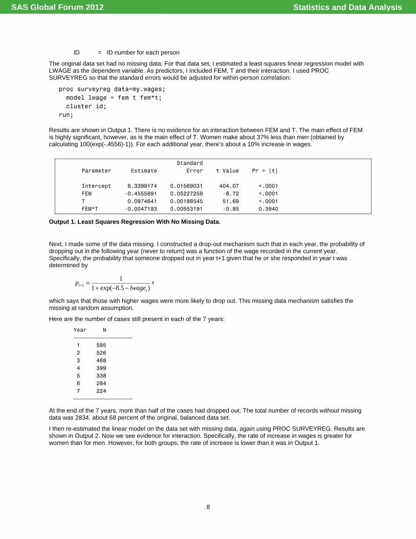
ID = ID number for each person

The original data set had no missing data. For that data set, I estimated a least-squares linear regression model with LWAGE as the dependent variable. As predictors, I included FEM, T and their interaction. I used PROC SURVEYREG so that the standard errors would be adjusted for within-person correlation:

proc surveyreg data=my.wages; model lwage = fem t fem*t; cluster id; run;

Results are shown in Output 1. There is no evidence for an interaction between FEM and T. The main effect of FEM is highly significant, however, as is the main effect of T. Women make about 37% less than men (obtained by calculating 100(exp(-.4556)-1)). For each additional year, there’s about a 10% increase in wages.

Standard Parameter Estimate Error t Value Pr > |t| Intercept 6.3399174 0.01569031 404.07 <.0001 FEM -0.4555891 0.05227259 -8.72 <.0001 T 0.0974641 0.00188545 51.69 <.0001 FEM*T -0.0047193 0.00553191 -0.85 0.3940

Output 1. Least Squares Regression With No Missing Data.

Next, I made some of the data missing. I constructed a drop-out mechanism such that in each year, the probability of dropping out in the following year (never to return) was a function of the wage recorded in the current year. Specifically, the probability that someone dropped out in year t+1 given that he or she responded in year t was determined by

)5.8exp(11

1t

t lwagep

−−+=+

,

which says that those with higher wages were more likely to drop out. This missing data mechanism satisfies the missing at random assumption.

Here are the number of cases still present in each of the 7 years:

Year N ƒƒƒƒƒƒƒƒƒƒƒƒƒƒƒƒƒƒ 1 595 2 526 3 468 4 399 5 338 6 284 7 224 ƒƒƒƒƒƒƒƒƒƒƒƒƒƒƒƒƒƒ

At the end of the 7 years, more than half of the cases had dropped out. The total number of records without missing data was 2834, about 68 percent of the original, balanced data set.

I then re-estimated the linear model on the data set with missing data, again using PROC SURVEYREG. Results are shown in Output 2. Now we see evidence for interaction. Specifically, the rate of increase in wages is greater for women than for men. However, for both groups, the rate of increase is lower than it was in Output 1.


9

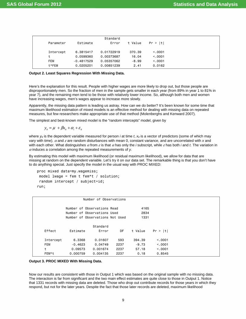
Standard Parameter Estimate Error t Value Pr > |t| Intercept 6.3815417 0.01722919 370.39 <.0001 t 0.0599360 0.00373687 16.04 <.0001 FEM -0.4817529 0.05357062 -8.99 <.0001 t*FEM 0.0205201 0.00851239 2.41 0.0162

Output 2. Least Squares Regression With Missing Data.

Here’s the explanation for this result. People with higher wages are more likely to drop out, but those people are disproportionately men. So the fraction of men in the sample gets smaller in each year (from 89% in year 1 to 81% in year 7), and the remaining men tend to be those with relatively lower income. So, although both men and women have increasing wages, men’s wages appear to increase more slowly.

Apparently, the missing data pattern is leading us astray. How can we do better? It’s been known for some time that maximum likelihood estimation of mixed models is an effective method for dealing with missing data on repeated measures, but few researchers make appropriate use of that method (Molenberghs and Kenward 2007).

The simplest and best-known mixed model is the “random intercepts” model, given by

itiitit xy εαβμ +++=

where yit is the dependent variable measured for person i at time t, xit is a vector of predictors (some of which may vary with time). α and ε are random disturbances with mean 0, constant variance, and are uncorrelated with x and with each other. What distinguishes α from ε is that α has only the i subscript, while ε has both i and t. The variation in α induces a correlation among the repeated measurements of y.

By estimating this model with maximum likelihood (or residual maximum likelihood), we allow for data that are missing at random on the dependent variable. Let’s try it on our data set. The remarkable thing is that you don’t have to do anything special. Just specify the model in the usual way with PROC MIXED:

proc mixed data=my.wagemiss; model lwage = fem t fem*t / solution; random intercept / subject=id; run;

Number of Observations Number of Observations Read 4165 Number of Observations Used 2834 Number of Observations Not Used 1331 Standard Effect Estimate Error DF t Value Pr > |t| Intercept 6.3368 0.01607 593 394.39 <.0001 FEM -0.4623 0.04749 2237 -9.73 <.0001 t 0.09573 0.001674 2237 57.18 <.0001 FEM*t 0.000759 0.004135 2237 0.18 0.8545

Output 3. PROC MIXED With Missing Data.

Now our results are consistent with those in Output 1 which was based on the original sample with no missing data. The interaction is far from significant and the two main effect estimates are quite close to those in Output 1. Notice that 1331 records with missing data are deleted. Those who drop out contribute records for those years in which they respond, but not for the later years. Despite the fact that those later records are deleted, maximum likelihood


10

“borrows” information from the values of the dependent variable in the earlier years to project what would happen in the later years. At the same time, it fully accounts for the uncertainty of this projection in the calculation of the standard errors and test statistics.

One could produce essentially the same results by doing multiple imputation. But it’s much simpler to handle the missing data problem with PROC MIXED.

A potential disadvantage of the random intercepts model is that it implies “exchangeability” or “compound symmetry”, which means that the correlation between values of the dependent variable at any two points in time will be the same for any pair of time points (after adjusting for covariates). In actuality, most longitudinal data sets show a pattern of decreasing correlations as the time points get farther apart. Molenberghs and Kenward (2007) argue that, for missing data applications, it’s very important to get the covariance structure right. So they recommend models that impose no structure on the covariances among the repeated measures.

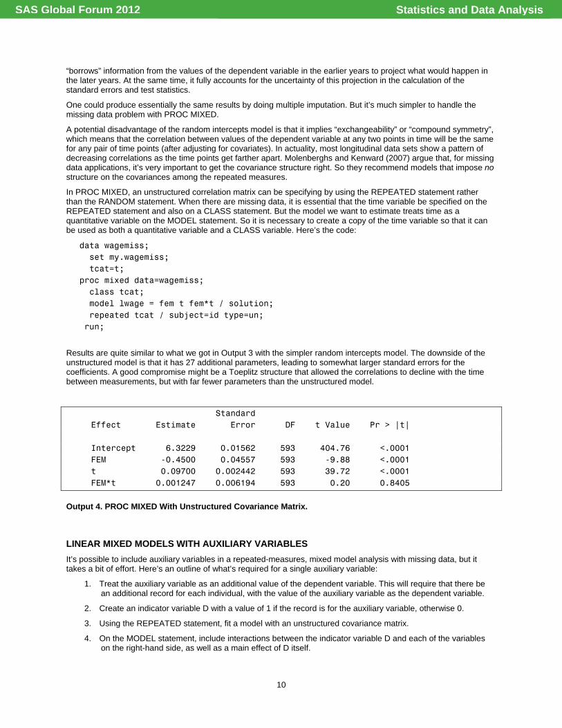
In PROC MIXED, an unstructured correlation matrix can be specifying by using the REPEATED statement rather than the RANDOM statement. When there are missing data, it is essential that the time variable be specified on the REPEATED statement and also on a CLASS statement. But the model we want to estimate treats time as a quantitative variable on the MODEL statement. So it is necessary to create a copy of the time variable so that it can be used as both a quantitative variable and a CLASS variable. Here’s the code:

data wagemiss; set my.wagemiss; tcat=t; proc mixed data=wagemiss; class tcat; model lwage = fem t fem*t / solution; repeated tcat / subject=id type=un; run;

Results are quite similar to what we got in Output 3 with the simpler random intercepts model. The downside of the unstructured model is that it has 27 additional parameters, leading to somewhat larger standard errors for the coefficients. A good compromise might be a Toeplitz structure that allowed the correlations to decline with the time between measurements, but with far fewer parameters than the unstructured model.

Standard Effect Estimate Error DF t Value Pr > |t| Intercept 6.3229 0.01562 593 404.76 <.0001 FEM -0.4500 0.04557 593 -9.88 <.0001 t 0.09700 0.002442 593 39.72 <.0001 FEM*t 0.001247 0.006194 593 0.20 0.8405

Output 4. PROC MIXED With Unstructured Covariance Matrix.

LINEAR MIXED MODELS WITH AUXILIARY VARIABLES

It’s possible to include auxiliary variables in a repeated-measures, mixed model analysis with missing data, but it takes a bit of effort. Here’s an outline of what’s required for a single auxiliary variable:

1. Treat the auxiliary variable as an additional value of the dependent variable. This will require that there be an additional record for each individual, with the value of the auxiliary variable as the dependent variable.

2. Create an indicator variable D with a value of 1 if the record is for the auxiliary variable, otherwise 0.

3. Using the REPEATED statement, fit a model with an unstructured covariance matrix.

4. On the MODEL statement, include interactions between the indicator variable D and each of the variables on the right-hand side, as well as a main effect of D itself.


11

In the output, the “main effects” of the variables will be the parameters of interest. The interactions are included simply to allow the independent variables to have different effects on the auxiliary variable.

MIXED MODELS WITH BINARY OUTCOMES

If the repeated-measures dependent variable is binary, you can get the same benefits with PROC GLIMMIX. Here’s an example. (The data used here come from clinical trials conducted as part of the National Drug Abuse Treatment Clinical Trials Network sponsored by National Institute on Drug Abuse). The sample consisted of 154 opioid-addicted youths, half of whom were randomly assigned to a treatment consisting of the administration of buprenorphine-naloxone over a 12-week period. The other half received a standard short-term detox therapy. The primary outcome of interest is a binary variable coded 1 if the subject tested positive for opiates. These urine tests were intended to be performed in each of the 12 weeks following randomization. However, for various reasons, there was a great deal of missing data on these outcomes. Twenty persons had missing data for all 12 outcomes, reducing the effective sample size to 134. After eliminating these 20 cases, Table 1 shows the proportion of cases with data present in each of the 12 weeks.

Week

Proportion

Present

1 .90

2 .74

3 .60

4 .78

5 .48

6 .45

7 .44

8 .69

9 .40

10 .37

11 .37

12 .67

Table 1. Proportion of cases with drug test data present in each of 12 weeks. The proportions were substantially higher in weeks 1, 4, 8, and 12, presumably because the subjects were paid $75 for participation in those weeks, but only $5 for participation in the other weeks. The objective is to estimate the effect of the treatment on the probability of a positive drug test, as well as evaluating how that effect may have changed over the 12-week period. We shall estimate a random effects (mixed) logit model using PROC GLIMMIX. Like PROC MIXED, GLIMMIX expects data in the “long form”, that is, one record for each longitudinal measurement for each individual. Thus, a person who was tested on all 12 occasions would have 12 records in the data set. Each record has an ID variable that has a unique value for each person and serves to link the separate records for each person. There is also a WEEK variable that records the week of the measurement (i.e., 1 through 12). Any variables that do not change over time (e.g., the treatment indicator) are simply replicated across the multiple observations for each person. If a person has a missing outcome at a particular time point, no record is necessary for that time point. Thus, a person who only was tested at weeks 1, 4, 8, and 12, has only four records in the data set. After some exploration, the best fitting model was a “random intercepts” logit model of the following form:


12

iiii

it

it ztttztzp

p αφθγδβμ ++++++=

−

22

1log

Here pit is the probability that person i tests positively for opiates at week t. zi is coded 1 if the person i is in the treatment group, otherwise 0. The model includes an interaction between treatment and week, a quadratic effect of week, and an interaction between treatment and week squared. αi represents all the causes of yi that vary across persons but not over time. It is assumed to be a random variable with the following properties:

• E(αi) = 0. • Var(αi) = τ2 • αi independent of xit and zi • αi normally distributed.

Here is the SAS code for estimating this model:

proc glimmix data=my.nidalong method=quad(qpoints=5); class usubjid; where week ne 0; model opiates=treat week week*treat week*week week*week*treat/ d=b solution ; random intercept / subject=usubjid; output out=a pred(ilink noblup)=yhat2 ; run;

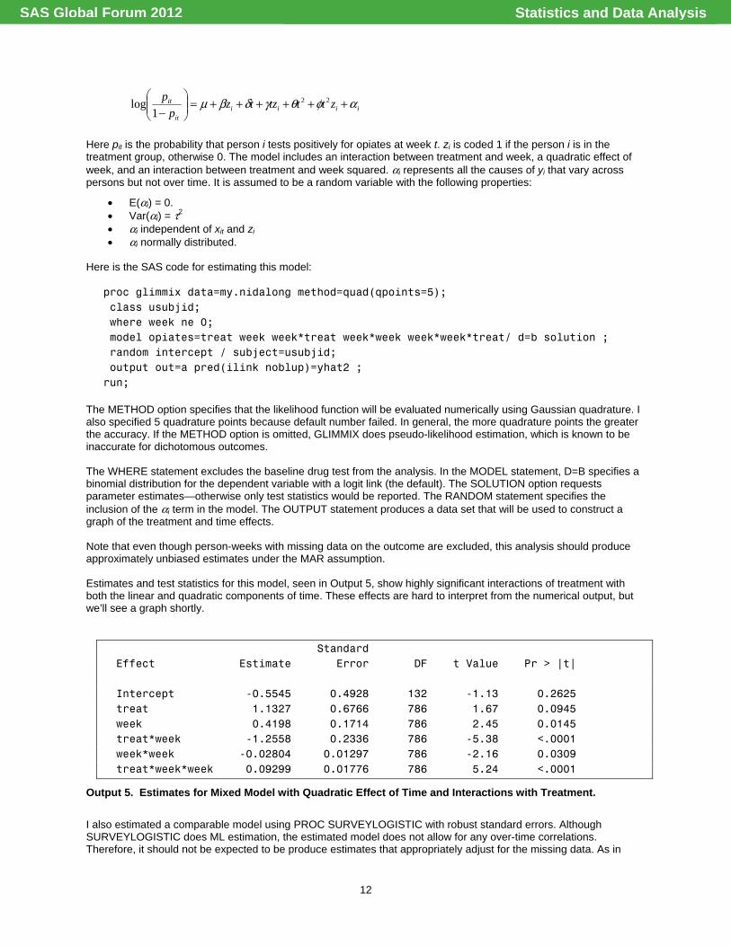
The METHOD option specifies that the likelihood function will be evaluated numerically using Gaussian quadrature. I also specified 5 quadrature points because default number failed. In general, the more quadrature points the greater the accuracy. If the METHOD option is omitted, GLIMMIX does pseudo-likelihood estimation, which is known to be inaccurate for dichotomous outcomes. The WHERE statement excludes the baseline drug test from the analysis. In the MODEL statement, D=B specifies a binomial distribution for the dependent variable with a logit link (the default). The SOLUTION option requests parameter estimates—otherwise only test statistics would be reported. The RANDOM statement specifies the inclusion of the αi term in the model. The OUTPUT statement produces a data set that will be used to construct a graph of the treatment and time effects. Note that even though person-weeks with missing data on the outcome are excluded, this analysis should produce approximately unbiased estimates under the MAR assumption. Estimates and test statistics for this model, seen in Output 5, show highly significant interactions of treatment with both the linear and quadratic components of time. These effects are hard to interpret from the numerical output, but we’ll see a graph shortly.

Standard Effect Estimate Error DF t Value Pr > |t| Intercept -0.5545 0.4928 132 -1.13 0.2625 treat 1.1327 0.6766 786 1.67 0.0945 week 0.4198 0.1714 786 2.45 0.0145 treat*week -1.2558 0.2336 786 -5.38 <.0001 week*week -0.02804 0.01297 786 -2.16 0.0309 treat*week*week 0.09299 0.01776 786 5.24 <.0001

Output 5. Estimates for Mixed Model with Quadratic Effect of Time and Interactions with Treatment.

I also estimated a comparable model using PROC SURVEYLOGISTIC with robust standard errors. Although SURVEYLOGISTIC does ML estimation, the estimated model does not allow for any over-time correlations. Therefore, it should not be expected to be produce estimates that appropriately adjust for the missing data. As in


13

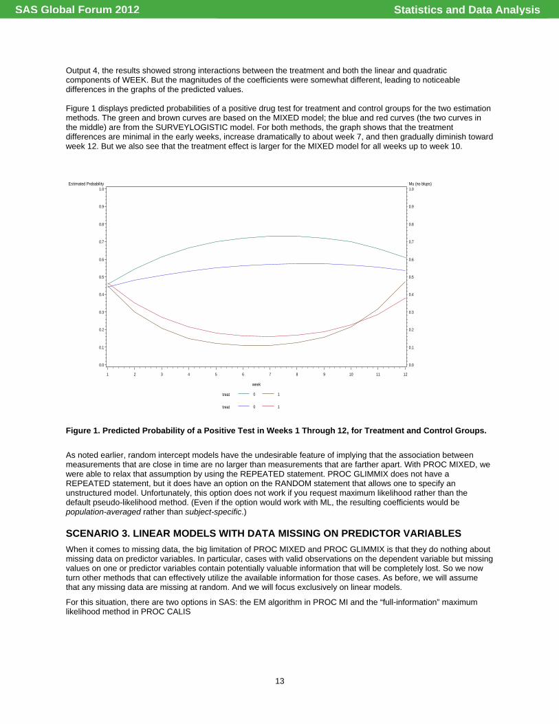
Output 4, the results showed strong interactions between the treatment and both the linear and quadratic components of WEEK. But the magnitudes of the coefficients were somewhat different, leading to noticeable differences in the graphs of the predicted values. Figure 1 displays predicted probabilities of a positive drug test for treatment and control groups for the two estimation methods. The green and brown curves are based on the MIXED model; the blue and red curves (the two curves in the middle) are from the SURVEYLOGISTIC model. For both methods, the graph shows that the treatment differences are minimal in the early weeks, increase dramatically to about week 7, and then gradually diminish toward week 12. But we also see that the treatment effect is larger for the MIXED model for all weeks up to week 10.

Estimated Probability

0.0

0.1

0.2

0.3

0.4

0.5

0.6

0.7

0.8

0.9

1.0

week

1 2 3 4 5 6 7 8 9 10 11 12

Mu (no blups)

0.0

0.1

0.2

0.3

0.4

0.5

0.6

0.7

0.8

0.9

1.0

treat 0 1

treat 0 1

Figure 1. Predicted Probability of a Positive Test in Weeks 1 Through 12, for Treatment and Control Groups.

As noted earlier, random intercept models have the undesirable feature of implying that the association between measurements that are close in time are no larger than measurements that are farther apart. With PROC MIXED, we were able to relax that assumption by using the REPEATED statement. PROC GLIMMIX does not have a REPEATED statement, but it does have an option on the RANDOM statement that allows one to specify an unstructured model. Unfortunately, this option does not work if you request maximum likelihood rather than the default pseudo-likelihood method. (Even if the option would work with ML, the resulting coefficients would be population-averaged rather than subject-specific.)

SCENARIO 3. LINEAR MODELS WITH DATA MISSING ON PREDICTOR VARIABLES

When it comes to missing data, the big limitation of PROC MIXED and PROC GLIMMIX is that they do nothing about missing data on predictor variables. In particular, cases with valid observations on the dependent variable but missing values on one or predictor variables contain potentially valuable information that will be completely lost. So we now turn other methods that can effectively utilize the available information for those cases. As before, we will assume that any missing data are missing at random. And we will focus exclusively on linear models.

For this situation, there are two options in SAS: the EM algorithm in PROC MI and the “full-information” maximum likelihood method in PROC CALIS


14

EM ALGORITHM IN PROC MI

Although PROC MI was designed primarily to do multiple imputation, the first step in the default algorithm is to do maximum likelihood estimation of the means and the covariance matrix using the EM algorithm. These estimates are used as starting values for the MCMC multiple imputation algorithm. But they can also be useful in their own right.

Consider the following example. The data set NLSYMISS (available at www.StatisticalHorizons.com), has records for 581 children who were surveyed in 1990 as part of the National Longitudinal Survey of Youth. Here are the variables:

ANTI antisocial behavior, measured with a scale ranging from 0 to 6.

SELF self-esteem, measured with a scale ranging from 6 to 24.

POV poverty status of family, coded 1 for in poverty, otherwise 0.

BLACK 1 if child is black, otherwise 0

HISPANIC 1 if child is Hispanic, otherwise 0

CHILDAGE child’s age in 1990

DIVORCE 1 if mother was divorced in 1990, otherwise 0

GENDER 1 if female, 0 if male

MOMAGE mother’s age at birth of child

MOMWORK 1 if mother was employed in 1990, otherwise 0

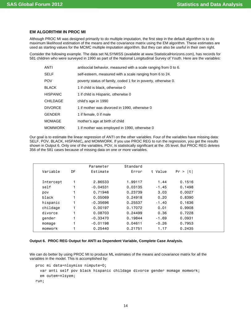
Our goal is to estimate the linear regression of ANTI on the other variables. Four of the variables have missing data: SELF, POV, BLACK, HISPANIC, and MOMWORK. If you use PROC REG to run the regression, you get the results shown in Output 6. Only one of the variables, POV, is statistically significant at the .05 level. But PROC REG deletes 356 of the 581 cases because of missing data on one or more variables.

Parameter Standard Variable DF Estimate Error t Value Pr > |t| Intercept 1 2.86533 1.99117 1.44 0.1516 self 1 -0.04531 0.03135 -1.45 0.1498 pov 1 0.71946 0.23739 3.03 0.0027 black 1 0.05069 0.24918 0.20 0.8390 hispanic 1 -0.35696 0.25537 -1.40 0.1636 childage 1 0.00197 0.17072 0.01 0.9908 divorce 1 0.08703 0.24499 0.36 0.7228 gender 1 -0.33470 0.19844 -1.69 0.0931 momage 1 -0.01198 0.04611 -0.26 0.7953 momwork 1 0.25440 0.21751 1.17 0.2435

Output 6. PROC REG Output for ANTI as Dependent Variable, Complete Case Analysis.

We can do better by using PROC MI to produce ML estimates of the means and covariance matrix for all the variables in the model. This is accomplished by:

proc mi data=nlsymiss nimpute=0; var anti self pov black hispanic childage divorce gender momage momwork; em outem=nlsyem; run;


15

The NIMPUTE=0 option suppresses multiple imputation. The EM statement requests EM estimates and writes the means and covariance matrix into a SAS data set called NLSYEM;

EM stands for expectation-maximization (Dempster et al. 1977). EM is simply a convenient numerical algorithm for getting ML estimates in certain situations under specified assumptions. In this case, the assumptions are that the data are missing at random, and all the variables have a multivariate normal distribution. That implies that every variable is a linear function of all the other variables (or any subset of them) with homoskedastic errors. I’ll have more to say about this assumption later.

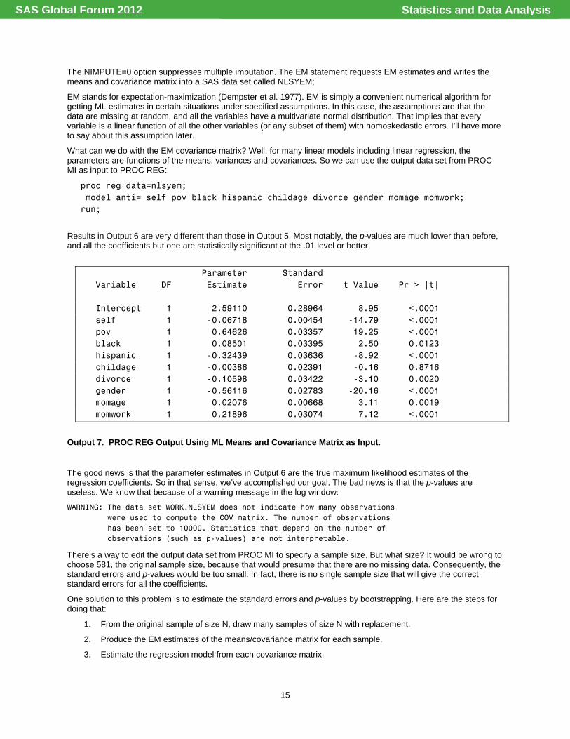
What can we do with the EM covariance matrix? Well, for many linear models including linear regression, the parameters are functions of the means, variances and covariances. So we can use the output data set from PROC MI as input to PROC REG:

proc reg data=nlsyem; model anti= self pov black hispanic childage divorce gender momage momwork; run;

Results in Output 6 are very different than those in Output 5. Most notably, the p-values are much lower than before, and all the coefficients but one are statistically significant at the .01 level or better.

Parameter Standard Variable DF Estimate Error t Value Pr > |t| Intercept 1 2.59110 0.28964 8.95 <.0001 self 1 -0.06718 0.00454 -14.79 <.0001 pov 1 0.64626 0.03357 19.25 <.0001 black 1 0.08501 0.03395 2.50 0.0123 hispanic 1 -0.32439 0.03636 -8.92 <.0001 childage 1 -0.00386 0.02391 -0.16 0.8716 divorce 1 -0.10598 0.03422 -3.10 0.0020 gender 1 -0.56116 0.02783 -20.16 <.0001 momage 1 0.02076 0.00668 3.11 0.0019 momwork 1 0.21896 0.03074 7.12 <.0001

Output 7. PROC REG Output Using ML Means and Covariance Matrix as Input.

The good news is that the parameter estimates in Output 6 are the true maximum likelihood estimates of the regression coefficients. So in that sense, we’ve accomplished our goal. The bad news is that the p-values are useless. We know that because of a warning message in the log window:

WARNING: The data set WORK.NLSYEM does not indicate how many observations were used to compute the COV matrix. The number of observations has been set to 10000. Statistics that depend on the number of observations (such as p-values) are not interpretable.

There’s a way to edit the output data set from PROC MI to specify a sample size. But what size? It would be wrong to choose 581, the original sample size, because that would presume that there are no missing data. Consequently, the standard errors and p-values would be too small. In fact, there is no single sample size that will give the correct standard errors for all the coefficients.

One solution to this problem is to estimate the standard errors and p-values by bootstrapping. Here are the steps for doing that:

1. From the original sample of size N, draw many samples of size N with replacement.

2. Produce the EM estimates of the means/covariance matrix for each sample.

3. Estimate the regression model from each covariance matrix.


16

4. Calculate the standard deviation of each regression coefficient across samples.

And here’s the SAS code for accomplishing that with 1000 bootstrap samples:

proc surveyselect data=nlsymiss method=urs n=581 reps=1000 out=bootsamp outhits; proc mi data=bootsamp nimpute=0 noprint; var anti self pov black hispanic childage divorce gender momage momwork; em outem=nlsyem; by replicate; proc reg data=nlsyem outest=a noprint; model anti= self pov black hispanic childage divorce gender momage momwork; by replicate; proc means data=a std; var self pov black hispanic childage divorce gender momage momwork; run;

Table 2 shows the ML coefficients (from Output 6), the bootstrapped standard errors, the z-statistics (ratios of coefficients to standard errors) and the associated p-values. Comparing this with Output 6—the complete case analysis—we see some major differences. SELF and GENDER are now highly significant, and HISPANIC and MOMWORK are now marginally significant. So ML really made a difference for this example.

Coefficient Std_Err z p

self -.06718 .022402 -2.99888 .0027097

pov .64626 .166212 3.888174 .000101

black .08501 .168117 .5056583 .6130966

hispanic -.32439 .163132 -1.988516 .0467547

childage -.00386 .103357 -.0373463 .9702089

divorce -.10598 .150277 -.705231 .4806665

gender -.56116 .114911 -4.883444 1.04e-06

momage .02076 .028014 .7410475 .4586646

momwork .21896 .145777 1.502024 .1330908

Table 2. ML Coefficients With Bootstrap Standard Errors.

This example had no auxiliary variables, but it would be easy to incorporate them into the analysis. Just add them to the VAR statement in PROC MI.

The primary weakness of this methodology is the assumption of multivariate normality for all the variables. That assumption can’t possibly be true for binary variables like POV, BLACK, HISPANIC and MOMWORK, all variables with missing data. However, that assumption is also the basis for the default MCMC method in PROC MI. So it’s no worse than multiple imputation in that regard. A considerable amount of simulation evidence suggests that violation of the multivariate normality assumption are not very problematic for multiple imputation (e.g., Schafer 1997, Allison 2006). Given the close similarity between multiple imputation and maximum likelihood under identical assumptions, I would expect ML to be robust to such violations also. However, toward the end of this paper, I will briefly discuss alternative ML methods with less restrictive assumptions.

FIML IN PROC CALIS

There’s an easier way to get the ML estimates in SAS, one that only requires a single procedure and does not require any additional computation to get the standard errors. Beginning with release 9.22, PROC CALIS can do what SAS calls “full information maximum likelihood” (FIML), which is just maximum likelihood estimation with appropriate incorporation of the cases with missing data. In other literature, the method is sometimes descibed as “direct” maximum likelihood (because it directly maximizes the likelihood for the specified model rather than doing the two


17

steps that we used with PROC MI) or “raw” maximum likelihood (because the model must be estimated using raw data rather than a covariance matrix).

First a little background. PROC CALIS is designed to estimate linear “structural equation models” (SEM), a very large class of linear models that involves multiple equations and often latent variables. It encompasses both the confirmatory factor model of psychometrics and the simultaneous equation model of econometrics. The SEM method was first introduced in the 1970s by Karl Jöreskog, who also developed the first stand-alone software package (called LISREL) to implement it.

Like most SEM software, the default estimation method in PROC CALIS is maximum likelihood under the assumption of multivariate normality. But the default is also to delete cases with missing data on any of the variables in the specified model. By specifying METHOD=FIML on the PROC statement, we can retain those cases by integrating the likelihood function over the variables with missing data. This results in a somewhat more complicated likelihood function, one that takes more computation to maximize.

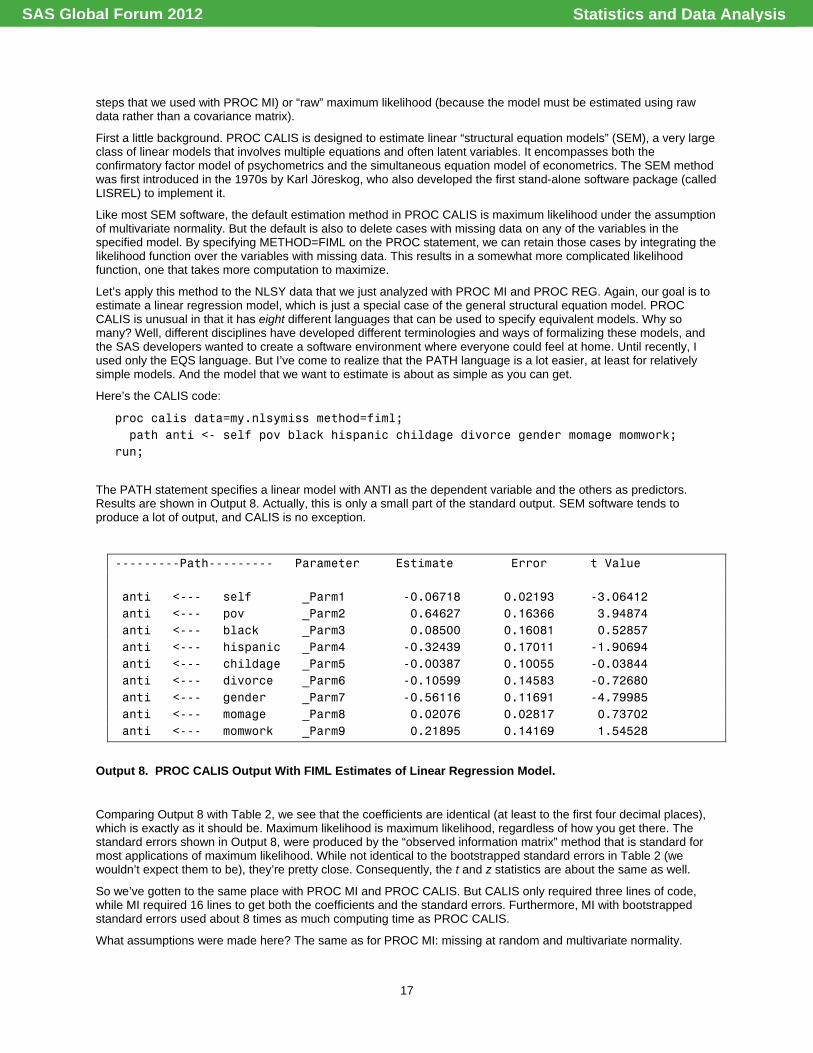
Let’s apply this method to the NLSY data that we just analyzed with PROC MI and PROC REG. Again, our goal is to estimate a linear regression model, which is just a special case of the general structural equation model. PROC CALIS is unusual in that it has eight different languages that can be used to specify equivalent models. Why so many? Well, different disciplines have developed different terminologies and ways of formalizing these models, and the SAS developers wanted to create a software environment where everyone could feel at home. Until recently, I used only the EQS language. But I’ve come to realize that the PATH language is a lot easier, at least for relatively simple models. And the model that we want to estimate is about as simple as you can get.

Here’s the CALIS code:

proc calis data=my.nlsymiss method=fiml; path anti <- self pov black hispanic childage divorce gender momage momwork; run;

The PATH statement specifies a linear model with ANTI as the dependent variable and the others as predictors. Results are shown in Output 8. Actually, this is only a small part of the standard output. SEM software tends to produce a lot of output, and CALIS is no exception.

---------Path--------- Parameter Estimate Error t Value anti <--- self _Parm1 -0.06718 0.02193 -3.06412 anti <--- pov _Parm2 0.64627 0.16366 3.94874 anti <--- black _Parm3 0.08500 0.16081 0.52857 anti <--- hispanic _Parm4 -0.32439 0.17011 -1.90694 anti <--- childage _Parm5 -0.00387 0.10055 -0.03844 anti <--- divorce _Parm6 -0.10599 0.14583 -0.72680 anti <--- gender _Parm7 -0.56116 0.11691 -4.79985 anti <--- momage _Parm8 0.02076 0.02817 0.73702 anti <--- momwork _Parm9 0.21895 0.14169 1.54528

Output 8. PROC CALIS Output With FIML Estimates of Linear Regression Model.

Comparing Output 8 with Table 2, we see that the coefficients are identical (at least to the first four decimal places), which is exactly as it should be. Maximum likelihood is maximum likelihood, regardless of how you get there. The standard errors shown in Output 8, were produced by the “observed information matrix” method that is standard for most applications of maximum likelihood. While not identical to the bootstrapped standard errors in Table 2 (we wouldn’t expect them to be), they’re pretty close. Consequently, the t and z statistics are about the same as well.

So we’ve gotten to the same place with PROC MI and PROC CALIS. But CALIS only required three lines of code, while MI required 16 lines to get both the coefficients and the standard errors. Furthermore, MI with bootstrapped standard errors used about 8 times as much computing time as PROC CALIS.

What assumptions were made here? The same as for PROC MI: missing at random and multivariate normality.


18

How can we incorporate auxiliary variables into the analysis? With PROC MI it was easy—just put the auxiliary variables on the VAR statement along with all the others. It’s a little more complicated with CALIS. Suppose we decide to remove SELF as a predictor in the linear regression model and treat it as an auxiliary variable instead. To do that properly, we must allow SELF to be freely correlated with all the variables in the regression model. An easy way to do that is to specify a second regression model with SELF as the dependent variable. Here’s how:

proc calis data=my.nlsymiss method=fiml; path anti <- pov black hispanic childage divorce gender momage momwork, self <- anti pov black hispanic childage divorce gender momage momwork; run;

Notice that the two “paths” or equations are separated by a comma, not a semicolon. Now suppose that we have two auxiliary variables rather than just one. Specifically, let’s remove MOMAGE from the main equation and treat it as an auxiliary variable:

proc calis data=my.nlsymiss method=fiml; path anti <- pov black hispanic childage divorce gender momwork, momage self <- anti pov black hispanic childage divorce gender momwork, momage <-> self; run;

The second line in the PATH statement has both MOMAGE and SELF on the left-hand side. This specifies two linear equations, one with MOMAGE as the dependent variable and the other with SELF as the dependent variable. But that’s not enough. We must also allow for a correlation between MOMAGE and SELF (or rather between their residuals). That’s accomplished with the third line in the PATH statement.

So that’s essentially how you use PROC CALIS to do ML estimation of a linear regression model when data are missing. But CALIS can do so much more than single equation linear regression. It can estimate confirmatory factor models, simultaneous equation models with feedback loops, and structural equation models with latent variables. For examples, see the paper by Yung and Zhang (2011) presented at last year’s Global Forum. As shown in my book Fixed Effects Regression Methods for Longitudinal Data Using SAS (2005), CALIS can also be used to estimate fixed and random effects models for longitudinal data. For any of these models, CALIS can handle missing data by maximum likelihood—as always, under the assumption of multivariate normality and missing at random.

SCENARIO 4. GENERALIZED LINEAR MODELS WITH DATA MISSING ON PREDICTORS

As we just saw, PROC CALIS can handle general patterns of missing data for almost any linear model that you might want to estimate. But suppose the dependent variable is dichotomous, and you want to estimate a logistic regression. Or maybe your dependent variable is a count of something, and you think that a negative binomial regression model would be more appropriate. If data are missing on predictors, there’s no SAS that can handle the missing data by maximum likelihood for these kinds of models. In that case, the best approach would be multiple imputation.

I know of only one commercial package that can do ML with missing predictors for generalized linear models, and that’s Mplus. Since this is a SAS forum, I won’t go into any of the details. But I do want to stress that Mplus can handle general patterns of missing data for an amazing variety of regression models: binary logistic, ordered logistic, multinomial logistic, poisson, negative binomial, tobit, and Cox regression. What’s more, with Mplus you can specify models that do not assume that the missing predictors have a multivariate normal distribution. Instead, you can model them as dependent variables using the same wide variety of regressions: logistic, poisson, etc. And you can do this for both cross-sectional and longitudinal data.

Hopefully, there will someday be a SAS procedure that can do this.

SCENARIO 5. DATA MISSING ON THE DEPENDENT VARIABLE, BUT NOT AT RANDOM

All the methods we have considered so far have been based on the assumption that the data are missing at random. That’s a strong assumption, but one that is not easy to relax. If you want to go the not-missing-at-random route, you must specify a model for the probability that data are missing as a function of both observed and unobserved variables. Such models are often not identified or may be only weakly identified.

Nevertheless, there is one such model that is widely used and can be estimated with PROC QLIM (part of the ETS product). It’s the “sample selection bias” model of James Heckman, who won the Nobel Prize in economics for this and other contributions.


19

Heckman’s (1976) model is not typically thought of us a missing data method, but that’s exactly what it is. The model is designed for situations in which the dependent variable in a linear regression model is missing for some cases but not for others. A common motivating example is a regression predicting women’s wages, where wage data are necessarily missing for women who are not in the labor force. It is natural to suppose that women are less likely to enter the labor force if their wages would be low upon entry. If that’s the case, the data are not missing at random.

Heckman formulated his model in terms of latent variables, but I will work with a more direct specification. For a sample of n cases (i=1,…, n), let Yi be a normally distributed variable with a variance σ2 and a conditional mean given by

E(Yi| Xi) = βXi

where Xi is a column vector of independent variables (including a value of 1 for the intercept) and β is a row vector of coefficients. The goal is to estimate β. If all Yi were observed, we could get ML estimates of β by ordinary least squares regression. But some Yi are missing. Let Ri be an indicator variable having a value of 1 if Y is observed and 0 if Yi is missing. The probability of missing data on Yi is assumed to follow a probit model

)(),|0Pr( 210 iiiii XYXYR ααα ++Φ==

where Φ(.) is the cumulative distribution function for a standard normal variable. If α1=0, the data are missing at random. Otherwise the data are not missing at random because the probability of missing Y depends on Y itself. If both α1=0 and α2=0, the data are missing completely at random.

This model is identified (even when there are no Xi or when Xi does not enter the probit equation) and can be estimated by maximum likelihood.

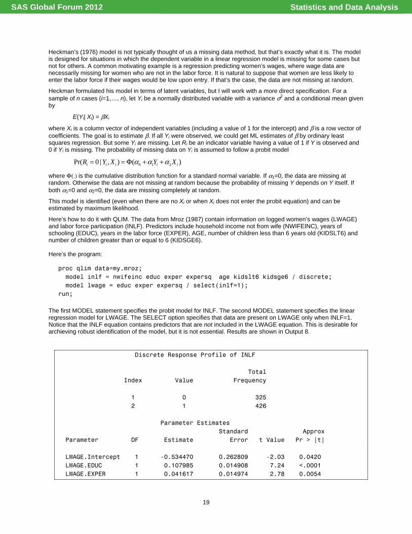
Here’s how to do it with QLIM. The data from Mroz (1987) contain information on logged women’s wages (LWAGE) and labor force participation (INLF). Predictors include household income not from wife (NWIFEINC), years of schooling (EDUC), years in the labor force (EXPER), AGE, number of children less than 6 years old (KIDSLT6) and number of children greater than or equal to 6 (KIDSGE6). Here’s the program:

proc qlim data=my.mroz; model inlf = nwifeinc educ exper expersq age kidslt6 kidsge6 / discrete; model lwage = educ exper expersq / select(inlf=1); run;

The first MODEL statement specifies the probit model for INLF. The second MODEL statement specifies the linear regression model for LWAGE. The SELECT option specifies that data are present on LWAGE only when INLF=1. Notice that the INLF equation contains predictors that are not included in the LWAGE equation. This is desirable for archieving robust identification of the model, but it is not essential. Results are shown in Output 8.

Discrete Response Profile of INLF Total Index Value Frequency 1 0 325 2 1 426 Parameter Estimates Standard Approx Parameter DF Estimate Error t Value Pr > |t| LWAGE.Intercept 1 -0.534470 0.262809 -2.03 0.0420 LWAGE.EDUC 1 0.107985 0.014908 7.24 <.0001 LWAGE.EXPER 1 0.041617 0.014974 2.78 0.0054


20

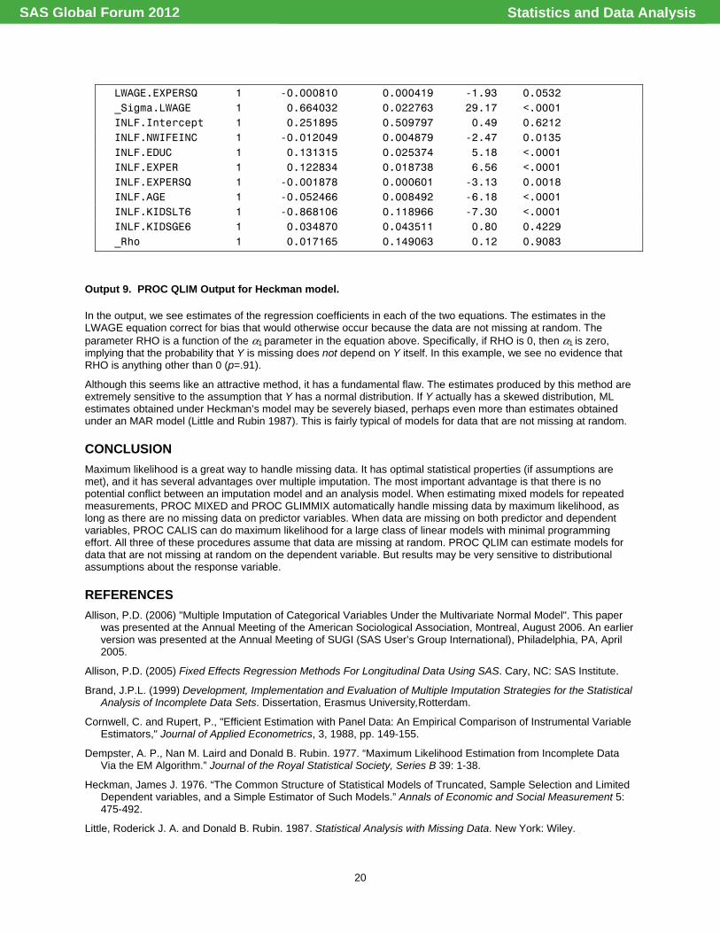
LWAGE.EXPERSQ 1 -0.000810 0.000419 -1.93 0.0532 _Sigma.LWAGE 1 0.664032 0.022763 29.17 <.0001 INLF.Intercept 1 0.251895 0.509797 0.49 0.6212 INLF.NWIFEINC 1 -0.012049 0.004879 -2.47 0.0135 INLF.EDUC 1 0.131315 0.025374 5.18 <.0001 INLF.EXPER 1 0.122834 0.018738 6.56 <.0001 INLF.EXPERSQ 1 -0.001878 0.000601 -3.13 0.0018 INLF.AGE 1 -0.052466 0.008492 -6.18 <.0001 INLF.KIDSLT6 1 -0.868106 0.118966 -7.30 <.0001 INLF.KIDSGE6 1 0.034870 0.043511 0.80 0.4229 _Rho 1 0.017165 0.149063 0.12 0.9083

Output 9. PROC QLIM Output for Heckman model.

In the output, we see estimates of the regression coefficients in each of the two equations. The estimates in the LWAGE equation correct for bias that would otherwise occur because the data are not missing at random. The parameter RHO is a function of the α1 parameter in the equation above. Specifically, if RHO is 0, then α1 is zero, implying that the probability that Y is missing does not depend on Y itself. In this example, we see no evidence that RHO is anything other than 0 (p=.91).

Although this seems like an attractive method, it has a fundamental flaw. The estimates produced by this method are extremely sensitive to the assumption that Y has a normal distribution. If Y actually has a skewed distribution, ML estimates obtained under Heckman’s model may be severely biased, perhaps even more than estimates obtained under an MAR model (Little and Rubin 1987). This is fairly typical of models for data that are not missing at random.

CONCLUSION

Maximum likelihood is a great way to handle missing data. It has optimal statistical properties (if assumptions are met), and it has several advantages over multiple imputation. The most important advantage is that there is no potential conflict between an imputation model and an analysis model. When estimating mixed models for repeated measurements, PROC MIXED and PROC GLIMMIX automatically handle missing data by maximum likelihood, as long as there are no missing data on predictor variables. When data are missing on both predictor and dependent variables, PROC CALIS can do maximum likelihood for a large class of linear models with minimal programming effort. All three of these procedures assume that data are missing at random. PROC QLIM can estimate models for data that are not missing at random on the dependent variable. But results may be very sensitive to distributional assumptions about the response variable.

REFERENCES

Allison, P.D. (2006) "Multiple Imputation of Categorical Variables Under the Multivariate Normal Model". This paper was presented at the Annual Meeting of the American Sociological Association, Montreal, August 2006. An earlier version was presented at the Annual Meeting of SUGI (SAS User’s Group International), Philadelphia, PA, April 2005.

Allison, P.D. (2005) Fixed Effects Regression Methods For Longitudinal Data Using SAS. Cary, NC: SAS Institute.

Brand, J.P.L. (1999) Development, Implementation and Evaluation of Multiple Imputation Strategies for the Statistical Analysis of Incomplete Data Sets. Dissertation, Erasmus University,Rotterdam.

Cornwell, C. and Rupert, P., "Efficient Estimation with Panel Data: An Empirical Comparison of Instrumental Variable Estimators," Journal of Applied Econometrics, 3, 1988, pp. 149-155.

Dempster, A. P., Nan M. Laird and Donald B. Rubin. 1977. “Maximum Likelihood Estimation from Incomplete Data Via the EM Algorithm.” Journal of the Royal Statistical Society, Series B 39: 1-38.

Heckman, James J. 1976. “The Common Structure of Statistical Models of Truncated, Sample Selection and Limited Dependent variables, and a Simple Estimator of Such Models.” Annals of Economic and Social Measurement 5: 475-492.

Little, Roderick J. A. and Donald B. Rubin. 1987. Statistical Analysis with Missing Data. New York: Wiley.


21

Molenberghs, G. and Kenward, M.G. (2007) Missing Data in Clinical Studies. Chichester, UK: John Wiley and Sons Ltd.

Mroz, T. A. (1987) “The sensitivity of an empirical model of married women's hours of work to economic and statistical assumptions.” Econometrica 55, 765–799.

Raghunathan, Trivellore E., James M. Lepkowski, John Van Hoewyk and Peter Solenberger (2001) “A multivariate technique for multiply imputing missing valuesusing a sequence of regression models.” Survey Methodology, 27: 85-95.

Rubin, Donald B. 1976. “Inference and Missing Data.” Biometrika 63: 581-592.

Rubin, Donald B. 1987. Multiple Imputation for Nonresponse in Surveys. New York: Wiley.

Schafer, Joseph L. 1997. Analysis of Incomplete Multivariate Data. London: Chapman & Hall.

Van Buuren, S., J.P.L. Brand, C.G.M. Groothuis-Oudshoorn and D.B. Rubin (2006) “Fully conditional specification in multivariate imputation.” Journal of Statistical Computation and Simulation 76: 1046-1064.

Van Buuren, S., and C.G.M. Oudshoorn (2000). Multivariate Imputation by Chained Equations: MICE V1.0 User’s Manual. Report PG/VGZ/00.038. Leiden: TNO Preventie en Gezondheid.

Yung, Y.F. and Zhang, W. (2011) “Making Use of Incomplete Observations in the Analysis of Structural Equation Models: The CALIS Procedure’s Full Information Maximum Likelihood Method in SAS/STAT® 9.3”. Paper 333-2011 presented at the SAS Global Forum.

CONTACT INFORMATION

Your comments and questions are valued and encouraged. Contact the author at:

Name: Paul D. Allison Enterprise: Statistical Horizons LLC Address: 530 New Gulph Rd. City, State ZIP: Haverford, PA 19041 Work Phone: 610-642-1941 Fax: 419-818-1220 E-mail: [email protected] Web: www.StatisticalHorizons.com

SAS and all other SAS Institute Inc. product or service names are registered trademarks or trademarks of SAS Institute Inc. in the USA and other countries. ® indicates USA registration.

Other brand and product names are trademarks of their respective companies.


312-2012: Handling Missing Data by Maximum Likelihood€¦ · 1 Paper 312-2012 Handling Missing...

Documents

Transcript of 312-2012: Handling Missing Data by Maximum Likelihood€¦ · 1 Paper 312-2012 Handling Missing...