1. INTRODUCTION3 2. ASSUMPTIONS6 3. …nielsen/soci709/cdocs/allison.pdf · novel approaches to...

ALLISON 1

TABLE OF CONTENTS

1. INTRODUCTION................................................................................................................. 3

2. ASSUMPTIONS.................................................................................................................... 6MISSING COMPLETELY AT RANDOM (MCAR) ............................................................................. 6MISSING AT RANDOM (MAR) ...................................................................................................... 7IGNORABLE .................................................................................................................................. 8NONIGNORABLE ........................................................................................................................... 8

3. CONVENTIONAL METHODS ........................................................................................ 10LISTWISE DELETION................................................................................................................... 10PAIRWISE DELETION .................................................................................................................. 13DUMMY VARIABLE ADJUSTMENT .............................................................................................. 14IMPUTATION............................................................................................................................... 16SUMMARY .................................................................................................................................. 17

4. MAXIMUM LIKELIHOOD.............................................................................................. 20REVIEW OF MAXIMUM LIKELIHOOD........................................................................................... 20ML WITH MISSING DATA........................................................................................................... 21CONTINGENCY TABLE DATA...................................................................................................... 23LINEAR MODELS WITH NORMALLY DISTRIBUTED DATA ........................................................... 26THE EM ALGORITHM................................................................................................................. 27EM EXAMPLE ............................................................................................................................ 29DIRECT ML................................................................................................................................ 31DIRECT ML EXAMPLE................................................................................................................ 33CONCLUSION.............................................................................................................................. 34

5. MULTIPLE IMPUTATION: BASICS ............................................................................. 42SINGLE RANDOM IMPUTATION................................................................................................... 42MULTIPLE RANDOM IMPUTATION .............................................................................................. 44ALLOWING FOR RANDOM VARIATION IN THE PARAMETER ESTIMATES...................................... 45MULTIPLE IMPUTATION UNDER THE MULTIVARIATE NORMAL MODEL ..................................... 47DATA AUGMENTATION FOR THE MULTIVARIATE NORMAL MODEL ........................................... 49CONVERGENCE IN DATA AUGMENTATION ................................................................................. 52SEQUENTIAL VS. PARALLEL CHAINS OF DATA AUGMENTATION ................................................ 53USING THE NORMAL MODEL FOR NON-NORMAL OR CATEGORICAL DATA................................ 55EXPLORATORY ANALYSIS .......................................................................................................... 57MI EXAMPLE 1........................................................................................................................... 58

6. MULTIPLE IMPUTATION: COMPLICATIONS ......................................................... 74INTERACTIONS AND NONLINEARITIES IN MI............................................................................... 74COMPATIBILITY OF THE IMPUTATION MODEL AND THE ANALYSIS MODEL................................ 76ROLE OF THE DEPENDENT VARIABLE IN IMPUTATION................................................................ 77USING ADDITIONAL VARIABLES IN THE IMPUTATION PROCESS ................................................. 78OTHER PARAMETRIC APPROACHES TO MULTIPLE IMPUTATION ................................................. 79

ALLISON 2

NON-PARAMETRIC AND PARTIALLY PARAMETRIC METHODS .................................................... 81SEQUENTIAL GENERALIZED REGRESSION MODELS.................................................................... 89LINEAR HYPOTHESIS TESTS AND LIKELIHOOD RATIO TESTS ..................................................... 91MI EXAMPLE 2........................................................................................................................... 95MI FOR LONGITUDINAL AND OTHER CLUSTERED DATA .......................................................... 100MI EXAMPLE 3......................................................................................................................... 102

7. NONIGNORABLE MISSING DATA............................................................................. 109TWO CLASSES OF MODELS....................................................................................................... 110HECKMAN’S MODEL FOR SAMPLE SELECTION BIAS................................................................. 112ML ESTIMATION WITH PATTERN-MIXTURE MODELS .............................................................. 114MULTIPLE IMPUTATION WITH PATTERN-MIXTURE MODELS .................................................... 116

NOTES ....................................................................................................................................... 121

REFERENCES.......................................................................................................................... 125

ALLISON 3

MISSING DATAPAUL D. ALLISONUniversity of Pennsylvania

1. INTRODUCTION

Sooner or later (usually sooner), anyone who does statistical analysis runs into problems

with missing data. In a typical data set, information is missing for some variables for some cases.

In surveys that ask people to report their income, for example, a sizeable fraction of the

respondents typically refuse to answer. But outright refusals are only one cause of missing data.

In self-administered surveys, people often overlook or forget to answer some of the questions.

Even trained interviewers may occasionally neglect to ask some questions. Sometimes

respondents say that they just don’t know the answer or don’t have the information available to

them. Sometimes the question is inapplicable for some respondents, as when asking unmarried

people to rate the quality of their marriage. In longitudinal studies, people who are interviewed in

one wave may die or move away before the next wave. When data are collated from multiple

administrative records, some records may have become inadvertently lost.

For all these reasons and many others, missing data is a ubiquitous problem in both the

social and health sciences. Why is it a problem? Because nearly all standard statistical methods

presume that every case has information on all the variables to be included in the analysis.

Indeed, the vast majority of statistical textbooks have nothing whatever to say about missing data

or how to deal with it.

There is one simple solution that everyone knows and that is usually the default for

statistical packages: if a case has any missing data for any of the variables in the analysis, then

ALLISON 4

simply exclude that case from the analysis. The result is a data set that has no missing data and

can be analyzed by any conventional method. This strategy is commonly known in the social

sciences as listwise deletion or casewise deletion, but also goes by the name of complete case

analysis.

Besides its simplicity, listwise deletion has some attractive statistical properties to be

discussed later on. But it also has a major disadvantage that is apparent to anyone who has used

it: in many applications, listwise deletion can exclude a large fraction of the original sample.

For example, suppose you have collected data on a sample of 1,000 people, and you want to

estimate a multiple regression model with 20 variables. Each of the variables has missing data

on five percent of the cases, and the chance that data is missing for one variable is independent

of the chance that it’s missing on any other variable. You could then expect to have complete

data for only about 360 of the cases, discarding the other 640. If you had merely downloaded the

data from a web site, you might not feel too bad about this, though you might wish you had a few

more cases. On the other hand, if you had spent $200 per interview for each of the 1,000 people,

you might have serious regrets about the $130,000 that was wasted (at least for this analysis).

Surely there must be some way to salvage something from the 640 incomplete cases, many of

which may lack data on only one of the 20 variables.

Many alternative methods have been proposed, and we will review several of them in this

book. Unfortunately, most of those methods have little value, and many of them are inferior to

listwise deletion. That’s the bad news. The good news is that statisticians have developed two

novel approaches to handling missing data—maximum likelihood and multiple imputation—that

offer substantial improvements over listwise deletion. While the theory behind these methods

has been known for at least a decade, it is only in the last few years that they have become

ALLISON 5

computationally practical. Even now, multiple imputation or maximum likelihood can demand a

substantial investment of time and energy, both in learning the methods and in carrying them out

on a routine basis. But hey, if you want to do things right, you usually have to pay a price.

Both maximum likelihood and multiple imputation have statistical properties that are

about as good as we can reasonably hope to achieve. Nevertheless, it’s essential to keep in mind

that these methods, like all the others, depend for their validity on certain assumptions that can

easily be violated. Not only that, for the most crucial assumptions, there’s no way to test

whether they are satisfied or not. The upshot is that while some missing data methods are clearly

better than others, none of them could really be described as “good”. The only really good

solution to the missing data problem is not to have any. So in the design and execution of

research projects, it’s essential to put great effort into minimizing the occurrence of missing data.

Statistical adjustments can never make up for sloppy research.

ALLISON 6

2. ASSUMPTIONS

Researchers often try to make the case that people who have missing values on a

particular variable are no different from those with observed measurements. It is common, for

example, to present evidence that people who do not report their income are not significantly

different from those who do, on a variety of other variables. More generally, researchers have

often claimed or assumed that their data are “missing at random” without a clear understanding

of what that means. Even statisticians were once vague or equivocal about this notion. In 1976,

however, Donald Rubin put things on a solid foundation by rigorously defining different

assumptions that one might plausibly make about missing data mechanisms. Although his

definitions are rather technical, I’ll try to convey an informal understanding of what they mean.

Missing Completely at Random (MCAR)

Suppose there is missing data on a particular variable Y. We say that the data on Y are

“missing completely at random” if the probability of missing data on Y is unrelated to the value

of Y itself or to the values of any other variables in the data set. When this assumption is

satisfied for all variables, the set of individuals with complete data can be regarded as a simple

random subsample from the original set of observations. Note that MCAR does allow for the

possibility that “missingness” on Y is related to “missingness” on some other variable X. For

example, even if people who refuse to report their age invariably refuse to report their income,

it’s still possible that the data could be missing completely at random.

The MCAR assumption would be violated if people who didn’t report their income were

younger, on average, than people who did report their income. It would be easy to test this

implication by dividing the sample into those who did and did not report their income, and then

ALLISON 7

testing for a difference in mean age. If there are, in fact, no systematic differences on the fully-

observed variables between those with data present and those with missing data, then we may

say that the data are observed at random. On the other hand, just because the data pass this test

doesn’t mean that the MCAR assumption is satisfied. There must still be no relationship

between missingness on a particular variable and the values of that variable.

While MCAR is a rather strong assumption, there are times when it is reasonable,

especially when data are missing as part of the research design. Such designs are often attractive

when a particular variable is very expensive to measure. The strategy then is to measure the

expensive variable for only a random subset of the larger sample, implying that data are missing

completely at random for the remainder of the sample.

Missing at Random (MAR)

A considerably weaker assumption is that the data are “missing at random”. We say that

data on Y are missing at random if the probability of missing data on Y is unrelated to the value

of Y, after controlling for other variables in the analysis. Here’s how to express this more

formally. Suppose we only have two variables X and Y, with X always observed and Y

sometimes missing. MAR means that

Pr(Y missing| Y, X) = Pr(Y missing| X).

In words is, the conditional probability of missing data on Y, given both Y and X, is equal to the

probability of missing data on Y given X alone. For example, the MAR assumption would be

satisfied if the probability of missing data on income depended on a person’s marital status but,

within each marital status category, the probability of missing income was unrelated to income.

In general, data are not missing at random if those with missing data on a particular variable tend

ALLISON 8

to have lower (or higher) values on that variable than those with data present, controlling for

other observed variables.

It’s impossible to test whether the MAR condition is satisfied, and the reason should be

intuitively clear. Since we don’t know the values of the missing data, we can’t compare the

values of those with and without missing data to see if they differ systematically on that variable.

Ignorable

We say that the missing data mechanism is ignorable if the (a) the data are MAR and (b)

the parameters governing the missing data process are unrelated to the parameters we want to

estimate. Ignorability basically means that we don’t need to model the missing data mechanism

as part of the estimation process. But we certainly do need special techniques to utilize the data

in an efficient manner. Because it’s hard to imagine real-world applications where condition (b)

is not satisfied, I treat MAR and ignorability as equivalent conditions in this book. Even in the

rare situation where condition (b) is not satisfied, methods that assume ignorability work just

fine; but you could do even better by modeling the missing data mechanism.

Nonignorable

If the data are not MAR, we say that the missing data mechanism is nonignorable. In that

case, we usually need to model the missing data mechanism to get good estimates of the

parameters of interest. One widely used method for nonignorable missing data is Heckman’s

(1976) two-stage estimator for regression models with selection bias on the dependent variable.

Unfortunately, for effective estimation with nonignorable missing data, we usually need very

good prior knowledge about the nature of the missing data process. That’s because the data

contain no information about what models would be appropriate, and the results will typically be

ALLISON 9

very sensitive to the choice of model. For this reason, and because models for nonignorable

missing data typically must be quite specialized for each application, this book puts the major

emphasis on methods for ignorable missing data. In the last chapter, I briefly survey some

approaches to handling nonignorable missing data. We shall also see that listwise deletion has

some very attractive properties with respect to certain kinds of nonignorable missing data.

ALLISON 10

3. CONVENTIONAL METHODS

While many different methods have been proposed for handling missing data, only a few

have gained widespread popularity. Unfortunately, none of the widely-used methods is clearly

superior to listwise deletion. In this section, I briefly review some of these methods, starting

with the simplest. In evaluating these methods, I will be particularly concerned with their

performance in regression analysis (including logistic regression, Cox regression, etc.), but many

of the comments also apply to other types of analysis as well.

Listwise Deletion

As already noted, listwise deletion is accomplished by deleting from the sample any

observations that have missing data on any variables in the model of interest, then applying

conventional methods of analysis for complete data sets. There are two obvious advantages to

listwise deletion: (1) it can be used for any kind of statistical analysis, from structural equation

modeling to loglinear analysis; (2) no special computational methods are required. Depending

on the missing data mechanism, listwise deletion can also have some attractive statistical

properties. Specifically, if the data are MCAR, then the reduced sample will be a random

subsample of the original sample. This implies that, for any parameter of interest, if the

estimates would be unbiased for the full data set (with no missing data), they will also be

unbiased for the listwise deleted data set. Furthermore, the standard errors and test statistics

obtained with the listwise deleted data set will be just as appropriate as they would have been in

the full data set.

Of course, the standard errors will generally be larger in the listwise deleted data set

because less information is utilized. They will also tend to be larger than standard errors

ALLISON 11

obtained from the optimal methods described later in this book. But at least you don’t have to

worry about making inferential errors because of the missing data—a big problem with most of

the other commonly-used methods.

On the other hand, if the data are not MCAR, but only MAR, listwise deletion can yield

biased estimates. For example, if the probability of missing data on schooling depends on

occupational status, regression of occupational status on schooling will produce a biased estimate

of the regression coefficient. So in general, it would appear that listwise deletion is not robust to

violations of the MCAR assumption. Surprisingly, however, listwise deletion is the method that

is most robust to violations of MAR among independent variables in a regression analysis.

Specifically, if the probability of missing data on any of the independent variables does not

depend on the values of the dependent variable, then regression estimates using listwise deletion

will be unbiased (if all the usual assumptions of the regression model are satisfied).1

For example, suppose that we want to estimate a regression model predicting annual

savings. One of the independent variables is income, for which 40% of the data are missing.

Suppose further that the probability of missing data on income is highly dependent on both

income and years of schooling, another independent variable in the model. As long as the

probability of missing income does not depend on savings, the regression estimates will be

unbiased (Little 1992).

Why is this the case? Here’s the essential idea. It’s well known that disproportionate

stratified sampling on the independent variables in a regression model does not bias coefficient

estimates. A missing data mechanism that depends only on the values of the independent

variables is essentially equivalent to stratified sampling. That is, cases are being selected into the

sample with a probability that depends on the values of those variables. This conclusion applies

ALLISON 12

not only to linear regression models, but also to logistic regression, Cox regression, Poisson

regression, and so on.

In fact, for logistic regression, listwise deletion gives valid inferences under even broader

conditions. If the probability of missing data on any variable depends on the value of the

dependent variable but does not depend on any of the independent variables, then logistic

regression with listwise deletion yields consistent estimates of the slope coefficients and their

standard errors. The intercept estimate will be biased, however. Logistic regression with

listwise deletion is only problematic when the probability of any missing data depends both on

the dependent and independent variables.2

To sum up, listwise deletion is not a bad method for handling missing data. Although it

does not use all of the available information, at least it gives valid inferences when the data are

MCAR. As we will see, that is more than can be said for nearly all the other commonplace

methods for handling missing data. The methods of maximum likelihood and multiple

imputation, discussed in later chapters, are potentially much better than listwise deletion in many

situations. But for regression analysis, listwise deletion is even more robust than these

sophisticated methods to violations of the MAR assumption. Specifically, whenever the

probability of missing data on a particular independent variable depends on the value of that

variable (and not the dependent variable), listwise deletion may do better than maximum

likelihood or multiple imputation.

There is one important caveat to these claims about listwise deletion for regression

analysis. We are assuming that the regression coefficients are the same for all cases in the

sample. If the regression coefficients vary across subsets of the population, then any nonrandom

restriction of the sample (e.g., through listwise deletion) may weight the regression coefficients

ALLISON 13

toward one subset or another. Of course, if we suspect such variation in the regression

parameters, we should either do separate regressions in different subsamples, or include

appropriate interactions in the regression model (Winship and Radbill 1994).

Pairwise Deletion

Also known as available case analysis, pairwise deletion is a simple alternative that can

be used for many linear models, including linear regression, factor analysis, and more complex

structural equation models. It is well known, for example, that a linear regression can be

estimated using only the sample means and covariance matrix or, equivalently, the means,

standard deviations and correlation matrix. The idea of pairwise deletion is to compute each of

these summary statistics using all the cases that are available. For example, to compute the

covariance between two variables X and Z, we use all the cases that have data present for both X

and Z. Once the summary measures have been computed, these can be used to calculate the

parameters of interest, for example, regression coefficients.

There are ambiguities in how to implement this principle. In computing a covariance,

which requires the mean for each variable, do you compute the means using only cases with data

on both variables, or do you compute them from all the available cases on each variable? There’s

no point in dwelling on such questions because all the variations lead to estimators with similar

properties. The general conclusion is that if the data are MCAR, pairwise deletion produces

parameter estimates that are consistent (and, therefore, approximately unbiased in large samples).

On the other hand, if the data are only MAR but not observed at random, the estimates may be

seriously biased.

If the data are indeed MCAR, we might expect pairwise deletion to be more efficient

than listwise deletion because more information is utilized. By more efficient, I mean that the

ALLISON 14

pairwise estimates would have less sampling variability (smaller true standard errors) than the

listwise estimates. That’s not always true, however. Both analytical and simulation studies of

linear regression models indicate that pairwise deletion produces more efficient estimates when

the correlations among the variables are generally low, while listwise does better when the

correlations are high (Glasser 1964, Haitovksty 1968, Kim and Curry 1977).

The big problem with pairwise deletion is that the estimated standard errors and test

statistics produced by conventional software are biased. Symptomatic of that problem is that

when you input a covariance matrix to a regression program, you must also specify the sample

size in order to calculate standard errors. Some programs for pairwise deletion use the number of

cases on the variable with the most missing data, while others use the minimum of the number of

cases used in computing each covariance. No single number is satisfactory, however. In

principle, it’s possible to get consistent estimates of the standard errors, but the formulas are

complex and have not been implemented in any commercial software.3

A second problem that occasionally arises with pairwise deletion, especially in small

samples, is that the constructed covariance or correlation matrix may not be “positive definite”,

which implies that the regression computations cannot be carried out at all. Because of these

difficulties, as well as its relative sensitivity to departures from MCAR, pairwise deletion cannot

be generally recommended as an alternative to listwise deletion.

Dummy Variable Adjustment

There is another method for missing predictors in a regression analysis that is remarkably

simple and intuitively appealing (Cohen and Cohen 1985). Suppose that some data are missing

on a variable X, is one of several independent variables in a regression analysis. We create a

ALLISON 15

dummy variable D which is equal to 1 if data are missing on X, otherwise 0. We also create a

variable X* such that

X* = X when data are not missing, and

X* = c when data are missing,

where c can be any constant. We then regress the dependent variable Y on X*, D, and any other

variables in the intended model. This technique, known as dummy variable adjustment or the

missing-indicator method, can easily be extended to the case of more than one independent

variable with missing data.

The apparent virtue of the dummy variable adjustment method is that it uses all the

information that is available about the missing data. The substitution of the value c for the

missing data is not properly regarded as imputation because the coefficient of X* is invariant to

the choice of c. Indeed, the only aspect of the model that depends on the choice of c is the

coefficient of D, the missing value indicator. For ease of interpretation, a convenient choice of c

is the mean of X for non-missing cases. Then the coefficient of D can be interpreted as the

predicted value of Y for individuals with missing data on X minus the predicted value of Y for

individuals at the mean of X, controlling for other variables in the model. The coefficient for X*

can be regarded as an estimate of the effect of X among the subgroup of those who have data on

X.

Unfortunately, this method generally produces biased estimates of the coefficients, as

proven by Jones (1996).4 Here’s a simple simulation that illustrates the problem. I generated

10,000 cases on three variables, X, Y, and Z, by sampling from a trivariate normal distribution.

For the regression of Y on X and Z, the true coefficients for each variable were 1.0. For the full

ALLISON 16

sample of 10,000, the least squares regression coefficients, shown in the first column of Table

3.1 are—not surprisingly—quite close to the true values.

I then randomly made some of the Z values missing with a probability of 1/2. Since the

probability of missing data is unrelated to any other variable, the data are MCAR. The second

column in Table 3.1 shows that listwise deletion yields estimates that are very close to those

obtained when no data are missing. On the other hand, the coefficients for the dummy variable

adjustment method are clearly biased—too high for the X coefficient and too low for the Z

coefficient.

TABLE 3.1 ABOUT HERE

A closely related method has been proposed for categorical independent variables in

regression analysis. Such variables are typically handled by creating a set of dummy variables,

one variable for each of the categories except for a reference category. The proposal is to simply

create an additional category—and an additional dummy variable—for those individuals with

missing data on the categorical variables. Again, however, we have an intuitively appealing

method that is biased even when the data are MCAR (Jones 1996, Vach and Blettner 1994).

Imputation

Many missing data methods fall under the general heading of imputation. The basic idea

is to substitute some reasonable guess (imputation) for each missing value, and then proceed to

do the analysis as if there were no missing data. Of course, there are lots of different ways to

impute missing values. Perhaps the simplest is marginal mean imputation: for each missing

value on a given variable, substitute the mean for those cases with data present on that variable.

This method is well known to produce biased estimates of variances and covariances (Haitovsky

1968) and should generally be avoided.

ALLISON 17

A better approach is use information on other variables by way of multiple regression, a

method sometimes knows as conditional mean imputation. Suppose we are estimating a multiple

regression model with several independent variables. One of those variables, X, has missing data

for some of the cases. For those cases with complete data, we regress X on all the other

independent variables. Using the estimated equation, we generate predicted values for the cases

with missing data on X. These are substituted for the missing data, and the analysis proceeds as

if there were no missing data.

The method gets more complicated when more than one independent variable has

missing data, and there are several variations on the general theme. In general, if imputations are

based solely on other independent variables (not the dependent variable) and if the data are

MCAR, least squares coefficients are consistent, implying that they are approximately unbiased

in large samples (Gourieroux and Monfort 1981). However, they are not fully efficient.

Improved estimators can be obtained using weighed least squares (Beale and Little 1975), or

generalized least squares (Gourieroux and Monfort 1981).

Unfortunately, all of these imputation methods suffer from a fundamental problem:

Analyzing imputed data as though it were complete data produces standard errors that are

underestimated and test statistics that are overestimated. Conventional analytic methods simply

do not adjust for the fact that the imputation process involves uncertainty about the missing

values.5 In later chapters, we will look at an approach to imputation that overcomes these

difficulties.

Summary

All the common methods for salvaging information from cases with missing data

typically make things worse. They either introduce substantial bias, make the analysis more

ALLISON 18

sensitive to departures from MCAR, or yield standard error estimates that are incorrect, usually

too low. In light of these shortcomings, listwise deletion doesn’t look so bad. But better

methods are available. In the next chapter we examine maximum likelihood methods that are

available for many common modeling objectives. In Chapters 5 and 6 we consider multiple

imputation, which can be used in almost any setting. Both methods have very good properties if

the data are MAR. In principle, these methods can also be used for nonignorable missing data,

but that requires a correct model of the process by which data are missing—something that’s

usually difficult to come by.

ALLISON 19

Table 3.1. Regression in Simulated Data for Three Methods

Coefficient of Full DataListwiseDeletion

Dummy VariableAdjustment

X .98 .96 1.28

Z 1.01 1.03 .87

D .02

ALLISON 20

4. MAXIMUM LIKELIHOOD

Maximum likelihood (ML) is very general approach to statistical estimation that is

widely used to handle many otherwise difficult estimation problems. Most readers will be

familiar with ML as the preferred method for estimating the logistic regression model. Ordinary

least squares linear regression is also an ML method when the error term is assumed to be

normally distributed. It turns out that ML is particularly adept at handling missing data

problems. In this chapter I begin by reviewing some general properties of ML estimates. Then I

present the basic principles of ML estimation under the assumption that the missing data

mechanism is ignorable. These principles are illustrated with a simple contingency table

example. The remainder of the chapter considers more complex examples where the goal is to

estimate a linear model, based on the multivariate normal distribution.

Review of Maximum Likelihood

The basic principle of ML estimation is to choose as estimates those values which, if true,

would maximize the probability of observing what has, in fact, been observed. To accomplish

this, we first need a formula that expresses the probability of the data as a function of both the

data and the unknown parameters. When observations are independent (the usual assumption),

the overall likelihood (probability) for the sample is just the product of all the likelihoods for the

individual observations.

Suppose we are trying to estimate a parameter θ . If f(y|θ) is the probability (or

probability density) of observing a single value of Y given some value of θ, the likelihood for a

sample of n observations is

∏=

=n

iiyfL

1

)|()( θθ

ALLISON 21

where Π is the symbol for repeated multiplication. Of course, we still need to specify exactly

what f(y|θ) is. For example, suppose Y is a dichotomous variable coded 1 or 0, and θ is the

probability that Y = 1. Then

yn

i

yL −

=

−= ∏ 1

1

)1()( θθθ

Once we have L(θ)—which is called the likelihood function—there are a variety of techniques to

find the value of θ that makes the likelihood as large as possible.

ML estimators have a number of desirable properties. Under a fairly wide range of

conditions, they are known to be consistent, asymptotically efficient and asymptotically normal

(Agresti and Finlay 1997). Consistency implies that the estimates are approximately unbiased in

large samples. Efficiency implies that the true standard errors are at least as small as the

standard errors for any other consistent estimators. The asymptotic part means that this

statement is only approximately true, with the approximation getting better as the sample size

gets larger. Finally, asymptotic normality means that in repeated sampling, the estimates have

approximately a normal distribution (again, with the approximation improving with increasing

sample size). This justifies the use a normal table in constructing confidence intervals or

computing p-values.

ML with Missing Data

What happens when data are missing for some of the observations? When the missing

data mechanism is ignorable (and hence MAR), we can obtain the likelihood simply by summing

the usual likelihood over all possible values of the missing data. Suppose, for example, that we

attempt to collect data on two variables, X and Y, for a sample of n independent observations.

For the first m observations, we observe both X and Y. But for the remaining n - m observations,

ALLISON 22

we are only able to measure Y. For a single observation with complete data, let’s represent the

likelihood by f(x,y|θ), where θ is a set of unknown parameters that govern the distribution of X

and Y. Assuming that X is discrete, the likelihood for a case with missing data on X is just the

“marginal” distribution of Y:

( ) ( )�=x

yxfyg θθ |,| .

(When X is continuous, the summation is replaced by an integral). The likelihood for the entire

sample is just

∏ ∏= +=

=m

i

n

miiii ygyxfL

1 1

)|()|,()( θθθ .

The problem then becomes one of finding values of θ to make this likelihood as large a possible.

A variety of methods are available to solve this optimization problem, and we’ll consider a few

of them later.

ML is particularly easy when the pattern of missing data is monotonic. In a monotonic

pattern, the variables can be arranged in order such that, for any observation in the sample, if

data are missing on a particular variable, they must also be missing for all variables that come

later in the order. Here’s an example with four variables, X1, X2, X3, and X4. There is no missing

data on X1. Ten percent of the cases are missing on X2. Those cases that are missing on X2 also

have missing data on X3 and X4. An additional 20% of the cases have missing data on both X3

and X4, but not on X2. A monotonic pattern often arises in panel studies, with people dropping

out at various points in time, never to return again.

If only one variable has missing data, the pattern is necessarily monotonic. Consider the

two-variable case with data missing on X only. The joint distribution f(x, y) can be written as

ALLISON 23

h(x | y)g(y) where g(y) is the marginal distribution of Y, defined above and h(x | y) is the

conditional distribution of X given Y. That enables us to rewrite the likelihood as

∏ ∏= =

=m

i

n

iygyxhL

1 1

)|();|(),( φλφλ .

This expression differs from the earlier one in two important ways. First, the second product is

over all the observations, not just those with missing data on X. Second, the parameters have

been separated into two parts: λ describes the conditional distribution of X given Y, and

φ describes the marginal distribution of Y. These changes imply that we can maximize the two

parts of the likelihood separately, typically using conventional estimation procedures for each

part. Thus, if X and Y have a bivariate normal distribution, we can calculate the mean and

variance of Y for the entire sample. Then, for those cases with data on X, we can calculate the

regression of X on Y. The resulting parameter estimates can be combined to produce ML

estimates for any other parameters we might be interested in, for example, the correlation

coefficient.

Contingency Table Data

These features of ML estimation can be illustrated very concretely with contingency table

data. Suppose for a simple random sample of 200 people, we attempt to measure two

dichotomous variables, X and Y, with possible values of 1 and 2. For 150 cases, we observe both

X and Y, with results shown in the following contingency table:

Y=1 Y=2X=1 52 21X=2 34 43

For the other 50 cases, X is missing and we observe only Y; specifically, we have 19 cases with

Y=1 and 31 cases with Y=2. In the population, the relationship between X and Y is described by

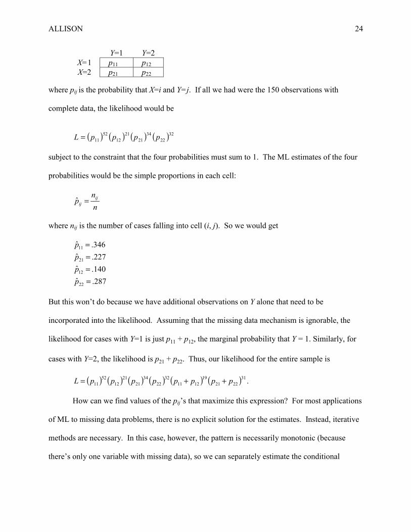
ALLISON 24

Y=1 Y=2X=1 p11 p12X=2 p21 p22

where pij is the probability that X=i and Y=j. If all we had were the 150 observations with

complete data, the likelihood would be

( ) ( ) ( ) ( )3222

3421

2112

5211 ppppL =

subject to the constraint that the four probabilities must sum to 1. The ML estimates of the four

probabilities would be the simple proportions in each cell:

nn

p ijij =ˆ

where nij is the number of cases falling into cell (i, j). So we would get

287.ˆ140.ˆ227.ˆ346.ˆ

22

12

21

11

====

pppp

But this won’t do because we have additional observations on Y alone that need to be

incorporated into the likelihood. Assuming that the missing data mechanism is ignorable, the

likelihood for cases with Y=1 is just p11 + p12, the marginal probability that Y = 1. Similarly, for

cases with Y=2, the likelihood is p21 + p22. Thus, our likelihood for the entire sample is

( ) ( ) ( ) ( ) ( ) ( )312221

191211

3222

3421

2112

5211 ppppppppL ++= .

How can we find values of the pij’s that maximize this expression? For most applications

of ML to missing data problems, there is no explicit solution for the estimates. Instead, iterative

methods are necessary. In this case, however, the pattern is necessarily monotonic (because

there’s only one variable with missing data), so we can separately estimate the conditional

ALLISON 25

distribution of X given Y, and the marginal distribution of Y. Then we combine the results to get

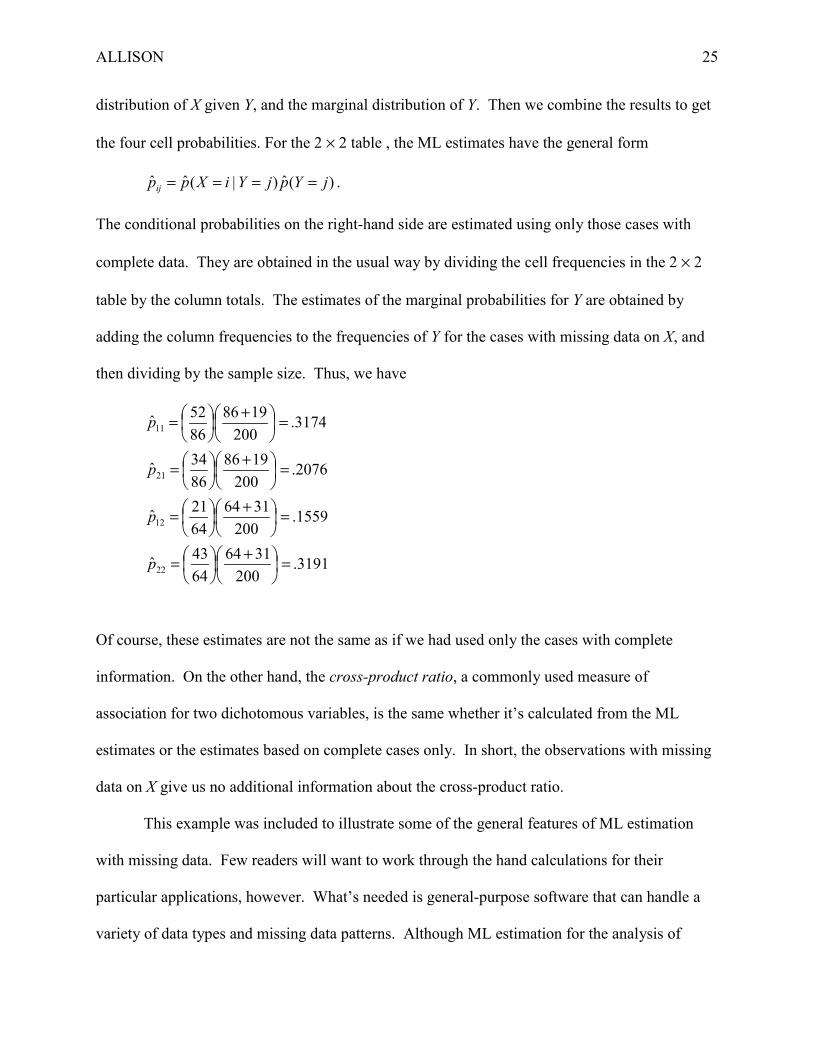
the four cell probabilities. For the 2 × 2 table , the ML estimates have the general form

)(ˆ)|(ˆˆ jYpjYiXppij ==== .

The conditional probabilities on the right-hand side are estimated using only those cases with

complete data. They are obtained in the usual way by dividing the cell frequencies in the 2 × 2

table by the column totals. The estimates of the marginal probabilities for Y are obtained by

adding the column frequencies to the frequencies of Y for the cases with missing data on X, and

then dividing by the sample size. Thus, we have

3191.200

31646443ˆ

1559.200

31646421ˆ

2076.200

19868634ˆ

3174.200

19868652ˆ

22

12

21

11

=��

��

� +��

��

�=

=��

��

� +��

��

�=

=��

��

� +��

��

�=

=��

��

� +��

��

�=

p

p

p

p

Of course, these estimates are not the same as if we had used only the cases with complete

information. On the other hand, the cross-product ratio, a commonly used measure of

association for two dichotomous variables, is the same whether it’s calculated from the ML

estimates or the estimates based on complete cases only. In short, the observations with missing

data on X give us no additional information about the cross-product ratio.

This example was included to illustrate some of the general features of ML estimation

with missing data. Few readers will want to work through the hand calculations for their

particular applications, however. What’s needed is general-purpose software that can handle a

variety of data types and missing data patterns. Although ML estimation for the analysis of

ALLISON 26

contingency tables is not computationally difficult (Fuchs 1982, Schafer 1997), there is virtually

no commercial software to handle this case. Freeware is available on the web, however:

� Jeroen K. Vermunt’s EM� program for Windows (http://cwis.kub.nl/~fsw_1/mto/mto3.htm)

estimates a wide variety of categorical data models when some data are missing.

� Joseph Schafer’s CAT program (http://www.stat.psu.edu/~jls) will estimate hierarchical

loglinear models with missing data, but is currently only available as a library for the S-

PLUS package.

� David Duffy’s LOGLIN program will estimate a variety of loglinear models with missing

data (http://www2.qimr.edu.au/davidD).

Linear Models with Normally Distributed Data

ML can be used to estimate a variety of linear models, under the assumption that the data

come from a multivariate normal distribution. Possible models include ordinary linear

regression, factor analysis, simultaneous equations, and structural equations with latent variables.

While the assumption of multivariate normality is a strong one, it is completely innocuous for

those variables with no missing data. Furthermore, even when some variables with missing data

are known to have distributions that are not normal (e.g., dummy variables), ML estimates under

the multivariate normal assumption often have good properties, especially if the data are

MCAR.6

There are several approaches to ML estimation for multivariate normal data with an

ignorable missing data mechanism. When the missing data follow a monotonic pattern, one can

take the approach described earlier of factoring the likelihood into conditional and marginal

distributions that can be estimated by conventional software (Marini, Olsen and Rubin 1979).

ALLISON 27

But this approach is very restricted in terms of potential applications, and it’s not easy to get

good estimates of standard errors and test statistics.

General missing data patterns can be handled by a method called the EM algorithm

(Dempster, Laird and Rubin 1977) which can produce ML estimates of the means, standard

deviations and correlations (or, equivalently, the means and the covariance matrix). These

summary statistics can then be input to standard linear modeling software to get consistent

estimates of the parameters of interest. The virtues of the EM method are, first, it’s easy to use

and, second, there is a lot of software that will do it, both commercial and freeware. But there

are two disadvantages: standard errors and test-statistics reported by the linear modeling software

will not be correct, and the estimates will not be fully efficient for over-identified models (those

which imply restrictions on the covariance matrix).

A better approach is direct maximization of the multivariate normal likelihood for the

assumed linear model. Direct ML (sometimes called “raw” maximum likelihood) gives efficient

estimates with correct standard errors, but requires specialized software that may have a steep

learning curve. In the remainder of the chapter, we’ll see how to use both the EM algorithm and

direct ML.

The EM Algorithm

The EM algorithm is a very general method for obtaining ML estimates when some of

the data are missing (Dempster et al.1977, McLachlan and Krishnan 1997). It’s called EM

because it consists of two steps: an Expectation step and a Maximization step. These two steps

are repeated multiple times in an iterative process that eventually converges to the ML estimates.

Instead of explaining the two steps of the EM algorithm in general settings, I’m going to

focus on its application to the multivariate normal distribution. Here the E-step essentially

ALLISON 28

reduces to regression imputation of the missing values. Let’s suppose our data set contains four

variables, X1 through X4, and there is some missing data on each variable, in no particular pattern.

We begin by choosing starting values for the unknown parameters, that is, the means and the

covariance matrix. These starting values could be obtained by the standard formulas for sample

means and covariances, using either listwise deletion or pairwise deletion. Based on the starting

values of the parameters, we can compute coefficients for the regression of any one of the X’s on

any subset of the other three. For example, suppose that some of the cases have data present for

X1 and X2 but not for X3 and X4. We use the starting values of the covariance matrix to get the

regression of X3 on X1 and X2 and the regression of X4 on X1 and X2. We then use these regression

coefficients to generate imputed values for X3 and X4 based on observed values of X1 and X2. For

cases with missing data on only one variable, we use regression imputations based on all three of

the other variables. For cases with data present for only one variable, the imputed value is just

the starting mean for that variable.

After all the missing data have been imputed, the M-step consists of calculating new

values for the means and the covariance matrix, using the imputed data along with the

nonmissing data. For means, we just use the usual formula. For variances and covariances,

modified formulas must be used for any terms involving missing data. Specifically, terms must

be added that correspond to the residual variances and residual covariances, based on the

regression equations used in the imputation process. For example, suppose that for observation i,

X3 was imputed using X1 and X2. Then, whenever (xi3)2 would be used in the conventional

variance formula, we substitute (xi3)2 + s23·21, where s2

3·21 is the residual variance from regressing

X3 on X1 and X2. The addition of the residual terms corrects for the usual underestimation of

variances that occurs in more conventional imputation schemes. Suppose X4 is also missing for

ALLISON 29

observation i. Then, when computing the covariance between X3 and X4, wherever xi3xi4 would be

used in the conventional covariance formula we substitute xi3xi4 + s34·21. The last term is the

residual covariance between X3 and X4, controlling for X1 and X2.

Once we’ve got new estimates for the means and covariance matrix, we start over with

the E-step. That is, we use the new estimates to produce new regression imputations for the

missing values. We keep cycling through the E- and M-steps until the estimates converge, that is,

they hardly change from one iteration to the next.

Note that the EM algorithm avoids one of the difficulties with conventional regression

imputation—deciding which variables to use as predictors and coping with the fact that different

missing data patterns have different sets of available predictors. Because EM always starts with

the full covariance matrix, it’s possible to get regression estimates for any set of predictors, no

matter how few cases there may be in a particular missing data pattern. Hence, it always uses all

the available variables as predictors for imputing the missing data.

EM Example

Data on 1,302 American colleges and universities were reported in the U.S. News and

World Report Guide to America’s Best Colleges 1994. These data can be found on the Web at

http://lib.stat.cmu.edu/datasets/colleges. We shall consider the following variables:

GRADRAT Ratio of graduating seniors to number enrolling four years earlier (× 100).

CSAT Combined average scores on verbal and math sections of the SAT.

LENROLL Natural logarithm of number of enrolling freshmen.

PRIVATE 1=private, 0=public.

STUFAC Ratio of students to faculty (× 100).

ALLISON 30

RMBRD Total annual costs for room and board (thousands of dollars).

ACT Mean ACT scores.

Our goal is to estimate a linear regression of GRADRAT on the next six variables. Although

ACT will not be in the regression model, it is included in the EM estimation because of its high

correlation with CSAT, a variable with substantial missing data, in order to get better

imputations for the missing values.


Table 4.1 gives the number of nonmissing cases for each variable, and the means and

standard deviations for those cases with data present. Only one variable, PRIVATE, has

complete data. The dependent variable GRADRAT has missing data on 8 percent of the

colleges. CSAT and RMBRD are each missing 40 percent, and ACT is missing 45 percent of the

cases. Using listwise deletion on all variables except ACT yields a sample of only 455 cases, a

clearly unacceptable reduction. Nevertheless, for purposes of comparison, listwise deletion

regression estimates are presented in Table 4.2.


Next we use the EM algorithm to get estimates of the means, standard deviations and

correlations. Among major commercial packages, the EM algorithm is available in BMDP,

SPSS, SYSTAT and SAS. However, with SPSS and SYSTAT, it is cumbersome to save the

results for input to other linear modeling routines. For the college data, I used the SAS procedure

MI to obtain the results shown in Tables 4.3 and 4.4. Like other EM software, this procedure

automates all the steps described in the previous section.


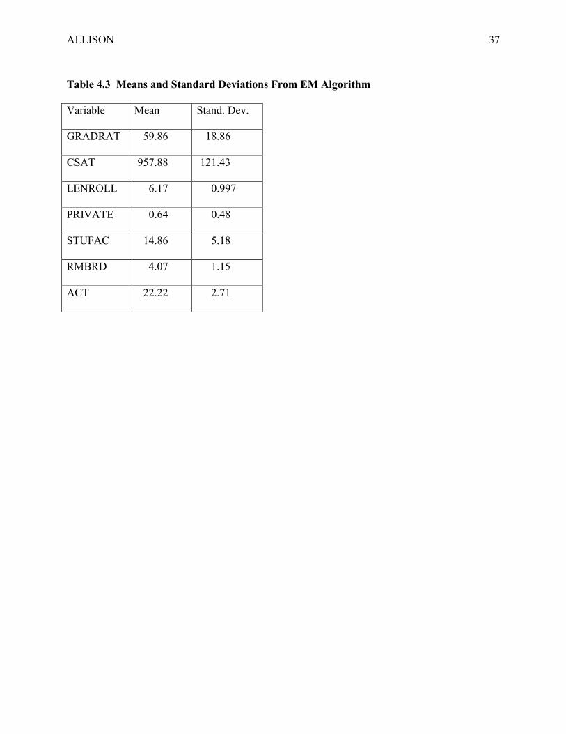
Comparing the means in Table 4.3 with those in Table 4.1, the biggest differences are

found—not surprisingly—among the variables with the most missing data: GRADRAT, CSAT,

ALLISON 31

RMBRD, and ACT. But even for these variables, none of the differences between listwise

deletion and EM exceeds two percent.


Table 4.5 shows regression estimates that use the EM statistics as input. While the

coefficients are not markedly different from those in Table 4.2 which used listwise deletion, the

reported standard errors are much lower, leading to higher t-statistics and lower p-values.

Unfortunately, while the coefficients are true ML estimates in this case, the standard error

estimates are undoubtedly too low because they assume that there is complete data for all the

cases. To get correct standard error estimates, we will use the direct ML method described

below.7


Direct ML

As we’ve just seen, most software for the EM algorithm produces estimates of the means

and an unrestricted correlation (or covariance) matrix. When those summary statistics are input

to other linear models programs, the resulting standard error estimates will be biased, usually

downward. To do better, we need to directly maximize the likelihood function for the model of

interest. This can be accomplished with any one of several software packages for estimating

structural equation models (SEMs) with latent variables.

When there are only a small number of missing data patterns, linear models can be

estimated with any SEM program that will handle multiple groups (Allison 1987, Muthén et al.

1987), including LISREL and EQS. For more general patterns of missing data, there are

currently four programs that perform direct ML estimation of linear models:

ALLISON 32

� Amos A commercial program for SEM modeling, available as a stand-alone package or

as a module for SPSS. Information is available at http://www.smallwaters.com.

� Mplus A stand-alone commercial program. Information is at http://www.statmodel.com.

� LINCS A commercial module for Gauss. Information is at http://www.aptech.com.

� Mx A freeware program available for download at http://views.vcu.edu/mx.

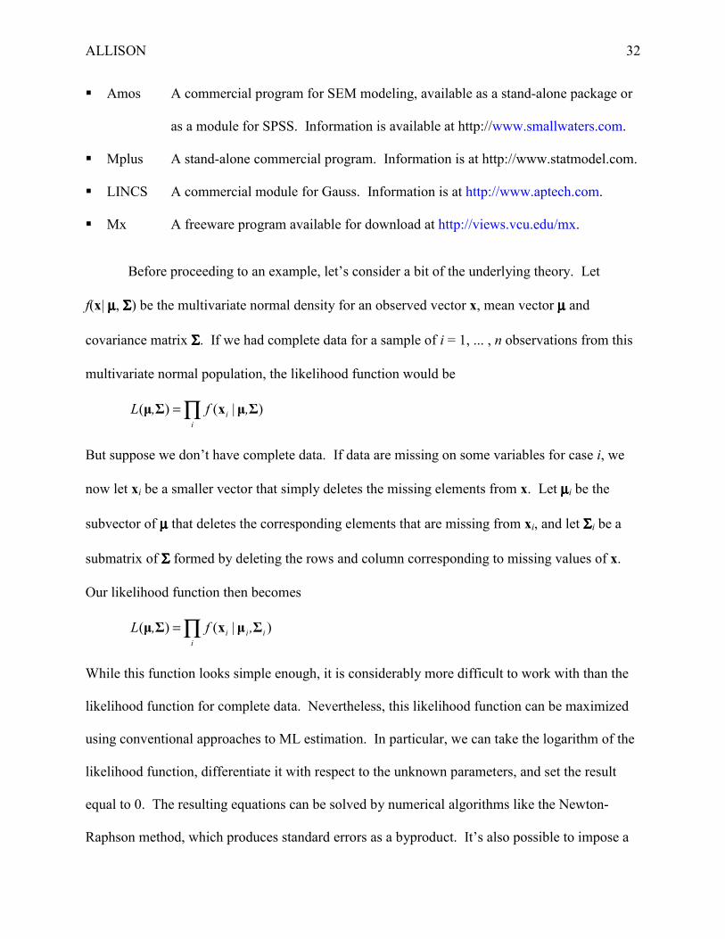
Before proceeding to an example, let’s consider a bit of the underlying theory. Let

f(x| µµµµ, ΣΣΣΣ) be the multivariate normal density for an observed vector x, mean vector µ µ µ µ and

covariance matrix ΣΣΣΣ. If we had complete data for a sample of i = 1, ... , n observations from this

multivariate normal population, the likelihood function would be

∏=i

i ,f,L )|()( ΣµxΣµ

But suppose we don’t have complete data. If data are missing on some variables for case i, we

now let xi be a smaller vector that simply deletes the missing elements from x. Let µµµµi be the

subvector of µ µ µ µ that deletes the corresponding elements that are missing from xi, and let ΣΣΣΣi be a

submatrix of Σ Σ Σ Σ formed by deleting the rows and column corresponding to missing values of x.

Our likelihood function then becomes

∏=i

iii ,f,L )|()( ΣµxΣµ

While this function looks simple enough, it is considerably more difficult to work with than the

likelihood function for complete data. Nevertheless, this likelihood function can be maximized

using conventional approaches to ML estimation. In particular, we can take the logarithm of the

likelihood function, differentiate it with respect to the unknown parameters, and set the result

equal to 0. The resulting equations can be solved by numerical algorithms like the Newton-

Raphson method, which produces standard errors as a byproduct. It’s also possible to impose a

ALLISON 33

structure on µ µ µ µ and ΣΣΣΣ by letting them be functions of a smaller set of parameters that correspond

to some assumed linear model. For example, the factor model sets

ΨΛΛΦΣ +′=

where ΛΛΛΛ is a matrix of factor loadings, ΦΦΦΦ is the covariance matrix of the latent factors, and ΨΨΨΨ is

the covariance matrix of the error components. The estimation process can produce ML

estimates of these parameters along with standard error estimates.

Direct ML Example

I estimated the college regression model using Amos 3.6, which has both a graphical user

interface and a text interface. The graphical interface allows the user to specify equations by

drawing arrows among the variables. But since I can’t show you a real-time demonstration, the

equivalent text commands are shown in Figure 4.1. The data were in a free-format text file

called COLLEGE.DAT, with missing values denoted by –9. The $MSTRUCTURE command

tells Amos to estimate means for the specified variables, an essential part of estimating models

with missing data. The $STRUCTURE command specifies the equation to be estimated. The

parentheses immediately after the equals sign indicates that an intercept is to be estimated. The

(1) ERROR at the end of the line tells Amos to include an error term with a coefficient of 1.0.

The last line, ACT<>ERROR, allows for a correlation between ACT and the error term, which is

possible because ACT has no direct effect on GRADRAT. Amos automatically allows for

correlations between ACT and the other independent variables in the regression equation.

FIGURE 4.1 ABOUT HERE

Results are shown in Table 4.6. Comparing these with the two-step EM estimates in

Table 4.5, we see that the coefficient estimates are identical, but the Amos standard errors are

ALLISON 34

noticeably larger—which is just what we would expect. They are still quite a bit smaller than

those in Table 4.2 obtained with listwise deletion.


Conclusion

Maximum likelihood can be an effective and practical method for handling data that are

missing at random. In this situation, ML estimates are known to be optimal in large samples.

For linear models that fall within the general class of structural equation models estimated by

programs like LISREL, ML estimates are easily obtained by several widely-available software

packages. Software is also available for ML estimation of loglinear models for categorical data,

but the implementation in this setting is somewhat less straightforward. One limitation of the

ML approach is that it requires a model for the joint distribution of all variables with missing

data. The multivariate normal model is often convenient for this purpose, but may be unrealistic

for many applications.

ALLISON 35

Table 4.1 Descriptive Statistics for College Data Based on Available Cases

VariableNonmissing

Cases MeanStandardDeviation

GRADRAT 1204 60.41 18.89

CSAT 779 967.98 123.58

LENROLL 1297 6.17 1.00

PRIVATE 1302 0.64 0.48

STUFAC 1300 14.89 5.19

RMBRD 783 4.15 1.17

ACT 714 22.12 2.58

ALLISON 36

Table 4.2 Regression Predicting GRADRAT Using Listwise Deletion

Variable Coefficient Standard Error t-statistic p-value

INTERCEP -35.028 7.685 -4.56 0.0001

CSAT 0.067 0.006 10.47 0.0001

LENROLL 2.417 0.959 2.52 0.0121

PRIVATE 13.588 1.946 6.98 0.0001

STUFAC -0.123 0.132 -0.93 0.3513

RMBRD 2.162 0.714 3.03 0.0026

ALLISON 37

Table 4.3 Means and Standard Deviations From EM Algorithm

Variable Mean Stand. Dev.

GRADRAT 59.86 18.86

CSAT 957.88 121.43

LENROLL 6.17 0.997

PRIVATE 0.64 0.48

STUFAC 14.86 5.18

RMBRD 4.07 1.15

ACT 22.22 2.71

ALLISON 38

Table 4.4 Correlations From EM Algorithm

GRADRAT CSAT LENROLL PRIVATE STUFAC RMBRD ACT

GRADRAT 1.000

CSAT 0.591 1.000

LENROLL -.027 0.192 1.000

PRIVATE 0.398 0.161 -.619 1.000

STUFAC -.318 -.315 0.267 -.368 1.000

RMBRD 0.478 0.479 -.016 0.340 -.282 1.000

ACT 0.598 0.908 0.174 0.224 -.293 0.484 1.000

ALLISON 39

Table 4.5 Regression Predicting GRADRAT, Based on EM Algorithm


INTERCEP -32.395 4.355 -7.44 0.0001

CSAT 0.067 0.004 17.15 0.0001

LENROLL 2.083 0.539 3.86 0.0001

PRIVATE 12.914 1.147 11.26 0.0001

STUFAC -0.181 0.084 -2.16 0.0312

RMBRD 2.404 .400 6.01 0.0001

ALLISON 40

Table 4.6 Regression Predicting GRADRAT Using Direct ML with Amos


INTERCEPT -32.395 4.863 -6.661 0.000000

CSAT 0.067 0.005 13.949 0.000000

LENROLL 2.083 0.595 3.499 0.000467

PRIVATE 12.914 1.277 10.114 0.000000

STUFAC -0.181 0.092 -1.968 0.049068

RMBRD 2.404 0.548 4.386 0.000012

ALLISON 41

Figure 4.1 Amos Commands for Regression Model Predicting GRADRAT.

$sample size=1302

$missing=-9

$input variables

gradrat

csat

lenroll

private

stufac

rmbrd

act

$rawdata

$include=c:\college.dat

$mstructure

csat

lenroll

private

stufac

rmbrd

act

$structure

gradrat=() + csat + lenroll + private + stufac + rmbrd + (1) error

act<>error

ALLISON 42

5. MULTIPLE IMPUTATION: BASICS

Although ML represents a major advance over conventional approaches to missing data,

it has its limitations. As we have seen, ML theory and software are readily available for linear

models and loglinear models but, beyond that, either theory or software is generally lacking. For

example, if you want to estimate a Cox proportional hazards model or an ordered logistic

regression model, you’ll have a tough time implementing ML methods for missing data. And

even if your model can be estimated with ML, you’ll need to use specialized software that may

lack diagnostics or graphical output that you particularly want.

Fortunately, there is an alternative approach—multiple imputation—that has the same

optimal properties as ML but removes some of these limitations. More specifically, multiple

imputation (MI), when used correctly, produces estimates that are consistent, asymptotically

efficient, and asymptotically normal when the data are MAR. But unlike ML, multiple

imputation can be used with virtually any kind of data and any kind of model. And the analysis

can be done with unmodified, conventional software. Of course MI has its own drawbacks. It

can be cumbersome to implement, and it’s easy to do it the wrong way. Both of these problems

can be substantially alleviated by using good software to do the imputations. A more

fundamental drawback is that MI produces different estimates (hopefully, only slightly different)

every time you use it. That can lead to awkward situations in which different researchers get

different numbers from the same data using the same methods.

Single Random Imputation

The reason that MI doesn’t produce a unique set of numbers is that random variation is

deliberately introduced in the imputation process. Without a random component, deterministic

ALLISON 43

imputation methods generally produce underestimates of variances for variables with missing

data and, sometimes, covariances as well. As we saw in the previous chapter, the EM algorithm

for the multivariate normal model solves that problem by using residual variance and covariance

estimates to correct the conventional formulas. However, a good alternative is to make random

draws from the residual distribution of each imputed variable, and add those random numbers to

the imputed values. Then, conventional formulas can be used for calculating variances and

covariances.

Here’s a simple example. Suppose we want to estimate the correlation between X and Y,

but data are missing on X for, say, 50 percent of the cases. We can impute values for the missing

X’s by regressing X on Y for the cases with complete data, and then using the resulting regression

equation to generate predicted values for the cases that are missing on X. I did this for a

simulated sample of 10,000 cases, where X and Y were drawn from a standard, bivariate normal

distribution with a correlation of .30. Half of the X values were assigned to be missing

(completely at random). Using the predicted values from the regression of X on Y to substitute

for the missing values, the correlation between X and Y was estimated to be .42.

Why the overestimate? The sample correlation is just the sample covariance of X and Y

divided by the product of their sample standard deviations. The regression imputation method

yields unbiased estimates of the covariance; moreover, the standard deviation of Y (with no

missing data) was correctly estimated at about 1.0. But the standard deviation of X (including

the imputed values) was only .74 while the true standard deviation was 1.0, resulting in an

overestimate of the correlation. An alternative way of thinking about the problem is that, for the

5,000 cases with missing data, the imputed value of X is a perfect linear function of Y, thereby

inflating the correlation between the two variables.

ALLISON 44

We can correct this bias by taking random draws from the residual distribution of X, then

adding those random numbers to the predicted values of X. In this example, the residual

distribution of X (regressed on Y) is normal with a mean of 0 and a standard deviation (estimated

from the listwise deleted least-squares regression) of .9525. For case i, let ui be a random draw

from a standard normal distribution, and let ix̂ be the predicted value from the regression of X on

Y. Our modified imputed value is then iii uxx 9525.ˆ~ += . For all observations in which X is

missing, we substitute ix~ , and then compute the correlation. When I did this for the simulated

sample of 10,000 cases, the correlation between X (with modified, imputed values) and Y was

.316, only a little higher than the true value of .300.

Multiple Random Imputation

Random imputation can eliminate the biases that are endemic to deterministic imputation.

But a serious problem remains. If we use imputed data (either random or deterministic) as if it

were real data, the resulting standard error estimates will generally be too low, and test statistics

will be too high. Conventional methods for standard error estimation can’t adequately account

for the fact that the data are imputed.

The solution, at least with random imputation, is to repeat the imputation process more

than once, producing multiple “completed” data sets. Because of the random component, the

estimates of the parameters of interest will be slightly different for each imputed data set. This

variability across imputations can be used to adjust the standard errors upward.


For the simulated sample of 10,000 cases, I repeated the random imputation process eight

times, yielding the estimates in Table 5.1. While these estimates are approximately unbiased, the

ALLISON 45

standard errors are downwardly biased because they don’t take account of the imputation.8 We

can combine the eight correlation estimates into a single estimate simply by taking their mean,

which is .3125. An improved estimate of the standard error takes three steps.

1. Square the estimated standard errors (to get variances) and average the results across the

eight replications.

2. Calculate the variance of the correlation estimates across the eight replications.

3. Add the results of steps 1 and 2 together (applying a small correction factor to the

variance in step 2) and take the square root.

To put this into one formula, let M be the number of replications, let rk be the correlation in

replication k, and let sk be estimated standard error in replication k. Then, the estimate of the

standard error of r (the mean of the correlation estimates), is

�� −��

��

�

−��

��

� ++=k

kk

k rrMM

sM

res 22 )(1

1111).(. (5.1)

This formula can be used for any parameter estimated by multiple imputation, with rk denoting

the k’th estimate of the parameter of interest (Rubin 1987). Applying this formula to the

correlation example, we get a standard error of .01123 which is about 24 percent higher than the

mean of the standard errors in the eight samples.

Allowing for Random Variation in the Parameter Estimates

Although the method I just described for imputing missing values is pretty good, it’s not

ideal. To generate the imputations for X, I regressed X on Y for the cases with complete data to

produce the regression equation

ii byax +=ˆ .

For cases with missing data on X, the imputed values were calculated as

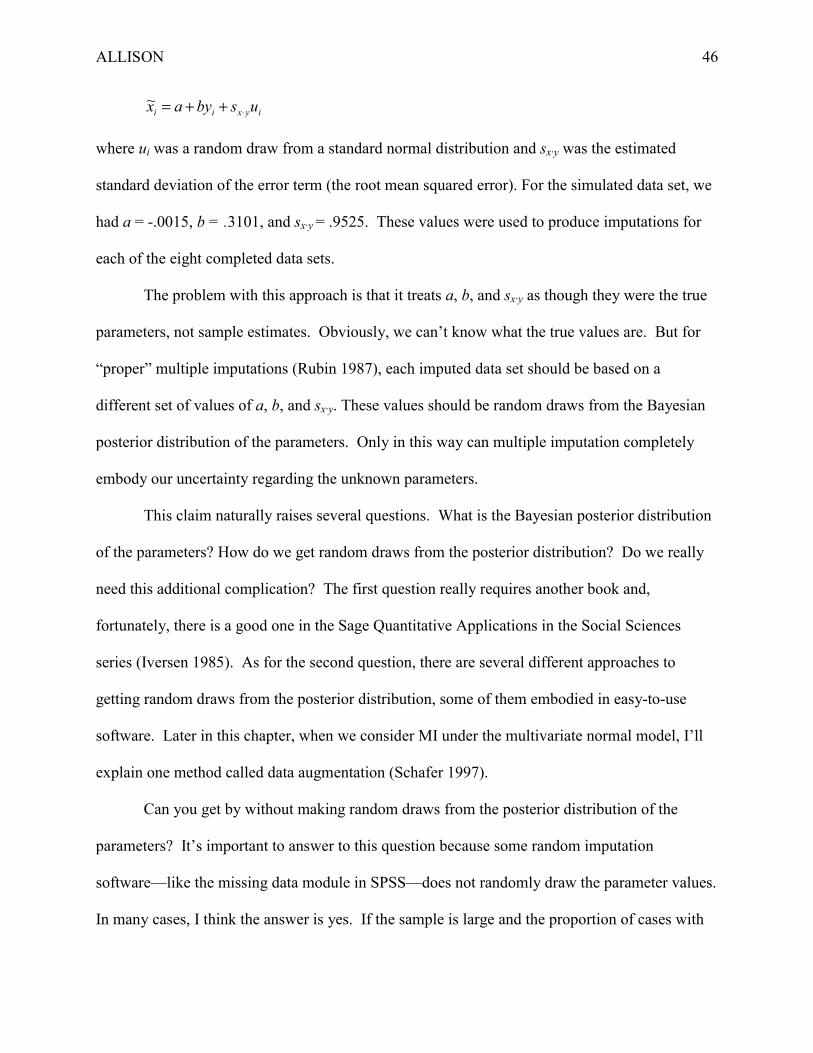
ALLISON 46

iyxii usbyax ⋅++=~

where ui was a random draw from a standard normal distribution and sx·y was the estimated

standard deviation of the error term (the root mean squared error). For the simulated data set, we

had a = -.0015, b = .3101, and sx·y = .9525. These values were used to produce imputations for

each of the eight completed data sets.

The problem with this approach is that it treats a, b, and sx·y as though they were the true

parameters, not sample estimates. Obviously, we can’t know what the true values are. But for

“proper” multiple imputations (Rubin 1987), each imputed data set should be based on a

different set of values of a, b, and sx·y. These values should be random draws from the Bayesian

posterior distribution of the parameters. Only in this way can multiple imputation completely

embody our uncertainty regarding the unknown parameters.

This claim naturally raises several questions. What is the Bayesian posterior distribution

of the parameters? How do we get random draws from the posterior distribution? Do we really

need this additional complication? The first question really requires another book and,

fortunately, there is a good one in the Sage Quantitative Applications in the Social Sciences

series (Iversen 1985). As for the second question, there are several different approaches to

getting random draws from the posterior distribution, some of them embodied in easy-to-use

software. Later in this chapter, when we consider MI under the multivariate normal model, I’ll

explain one method called data augmentation (Schafer 1997).

Can you get by without making random draws from the posterior distribution of the

parameters? It’s important to answer to this question because some random imputation

software—like the missing data module in SPSS—does not randomly draw the parameter values.

In many cases, I think the answer is yes. If the sample is large and the proportion of cases with

ALLISON 47

missing data is small, MI without this extra step will typically yield results that are very close to

those obtained with it. On the other hand, if the sample is small or if the proportion of cases with

missing data is large, the additional variation can make a noticeable difference.

Continuing our correlation example, I imputed eight new data sets using the data

augmentation method to generate random draws from the posterior distribution of the

parameters. Table 5.2 gives the correlation between X and Y and its standard error for each data

set. The mean of the correlation estimates is .31288. Using formula (5.1), the estimated

standard error is .01329, slightly larger than the .01123 obtained with the cruder imputation

method. In general, the standard errors will be somewhat larger when the parameters used in the

imputation are randomly drawn.


Multiple Imputation Under the Multivariate Normal Model

To do multiple imputation, you need a model for generating the imputations. For the two-

variable example just considered, I employed a simple regression model with normally

distributed errors. Obviously, more complicated situations require more complicated models. As

we saw in Chapter 4, maximum likelihood also requires a model. But MI is probably less

sensitive than ML to the choice of model because the model is used only for imputing the

missing data, not for estimating other parameters.

Ideally, the imputation model would be specially constructed to represent the particular

features of each data set. In practice, it is more convenient to work with “off-the-shelf” models

that are easy to use and provide reasonably good approximations for a wide range of data sets.

The most popular model for MI is the multivariate normal model, previously used in

ALLISON 48

Chapter 4 as the basis for ML estimation of linear models with missing data. The multivariate

normal model implies that

� all variables have normal distributions;

� each variable can be represented as a linear function of all the other variables,

together with a normal, homoscedastic error term.

Although these are strong conditions, in practice the multivariate normal model seems to do a

good job of imputation even when some of the variables have distributions that are manifestly

not normal (Schafer 1997). It is a completely innocuous assumption for those variables that have

no missing data. And for those variables that do have missing data, normalizing transformations

can greatly improve the quality of the imputations.

In essence, MI under the multivariate normal model is a generalization of the method

used in the two-variable example of the previous section. For each variable with missing data,

we estimate the linear regression of that variable on all other variables of interest. Ideally, the

regression parameters are random draws from the Bayesian posterior distribution. The estimated

regression equations are then used to generate predicted values for the cases with missing data.

Finally, to each predicted value, we add a random draw from the residual normal distribution for

that variable.

The most complicated part of the imputation process is getting random draws from the

posterior distribution of the regression parameters. As of this writing, two algorithms for

accomplishing this have been implemented in readily available software: data augmentation

(Schafer 1997) and sampling importance/resampling (SIR) (Rubin 1987). Here are some

computer programs that implement these methods:

ALLISON 49

Data Augmentation

NORM A freeware package developed by J.L. Schafer and described in his 1997 book,

available in either a stand-alone Windows version or as an Splus library

(http://www.stat.psu.edu/~jls/).

SOLAS A stand-alone commercial package that includes both data augmentation (version 2

and later) and a propensity score method. The latter method is invalid for many

applications (Allison 2000). (http://www.statsolusa.com)

PROC MI A SAS procedure available in release 8.1 and later. (http://www.sas.com)

Sampling Importance/Resampling (SIR)

AMELIA A freeware package developed by King, Honaker, Joseph, Scheve and Singh

(1999), available either as a stand-alone Windows program or as a module for

Gauss. (http://gking.harvard.edu/stats.shtml)

SIRNORM A SAS macro written by C. H. Brown and X. Ling.

(http://yates.coph.usf.edu/research/psmg/sirnorm/sirnorm.html)

Both algorithms have some theoretical justification. Proponents of SIR (King et al. 2000) claim

that it requires far less computer time. But the relative superiority of these two methods is far

from settled. Because I have much more experience with data augmentation, I’ll focus on that

method in the remainder of this chapter.

Data Augmentation for the Multivariate Normal Model

Data augmentation (DA) is a type of Markov Chain Monte Carlo (MCMC) algorithm, a

general method for finding posterior distributions that has become increasingly popular in

Bayesian statistics. In this section, I’ll describe how it works for the multivariate normal model.

ALLISON 50

Although the available software performs most of the operations automatically, it’s helpful to

have a general idea of what’s going on, especially when things go wrong.

The general structure of the iterative algorithm is much like the EM algorithm for the

multivariate normal model, described in the last chapter, except that random draws are made at

two points, described below. Before beginning DA, it’s necessary to choose a set of variables

for the imputation process. Obviously this should include all variables with missing data, as well

as other variables in the model to be estimated. It’s also worthwhile including additional

variables (not in the intended model) that are highly correlated with the variables that have

missing data, or that are associated with the probability that those variables have missing data.

Once the variables are chosen, DA consists of the following steps.

1. Choose starting values for the parameters. For the multivariate normal model, the parameters

are the means and the covariance matrix. Starting values can be gotten from standard

formulas using listwise deletion or pairwise deletion. Even better are the estimates obtained

with the EM algorithm, described in the last chapter.

2. Use the current values of the means and covariances to obtain estimates of regression

coefficients for equations in which each variable with missing data is regressed on all

observed variables. This is done for each pattern of missing data.

3. Use the regression estimates to generate predicted values for all the missing values. To each

predicted value, add a random draw from the residual normal distribution for that variable.

4. Using the “completed” data set, with both observed and imputed values, recalculate the

means and covariance matrix using standard formulas.

5. Based on the newly-calculated means and covariances, make a random draw from the

posterior distribution of the means and covariances.

ALLISON 51

6. Using the randomly drawn means and covariances, go back to step 2, and continue cycling

through the subsequent steps until convergence is achieved. The imputations that are

produced during the final iteration are used to form a completed data set.

Step 5 needs a little more explanation. To get the posterior distribution of the parameters,

we first need a “prior” distribution. Although this can be based on prior beliefs about those

parameters, the usual practice is to use a “noninformative” prior, that is, a prior distribution that

contains little or no information about the parameters. Here’s how it works in a simple situation.

Suppose we have a sample of size n with measurements on a single, normally distributed

variable Y. The sample mean is y and the sample variance is s2. We want random draws from

the posterior distribution of µ and σ2. With a noninformative prior9, we can get 2~σ , a random

draw for the variance, by sampling from a chi-square distribution with n-1 degrees of freedom,

taking the reciprocal of the drawn value and multiplying the result by ns2. We then get a random

draw for the mean by sampling from a normal distribution with mean y and variance 2~σ /n.

If there were no missing data, these would be random draws from the true posterior

distribution of the parameters. But if we’ve imputed any missing data, what we actually have are

random draws from the posterior distribution that would result if the imputed data were the true

data. Similarly, when we randomly impute missing data in step 3, what we have are random

draws from the posterior distribution of the missing data, given the current parameter values.

But since the current values may not be the true values, the imputed data may not be random

draws from the true posterior distribution. That’s why the procedure must be iterative. By

continually moving back and forth between random draws of parameters (conditional on both

observed and imputed data) and random draws of the missing data (conditional on the current

ALLISON 52

parameters), we eventually get random draws from the joint posterior distribution of both data

and parameters, conditioning only on the observed data.

Convergence in Data Augmentation

When you do data augmentation, you must specify the number of iterations. But that

raises a tough question: How many iterations are necessary to get convergence to the joint

posterior distribution of missing data and parameters? With iterative estimation for maximum

likelihood, as in the EM algorithm, the estimates converge to a single set of values. Convergence

can then be easily assessed by checking to see how much change there is in the parameter

estimates from one iteration to the next. For data augmentation, on the other hand, the algorithm

converges to a probability distribution, not a single set of values. That makes it rather difficult to

determine whether convergence has, in fact, been achieved. Although some diagnostic statistics

are available for assessing convergence (Schafer 1997), they are far from definitive.

In most applications, the choice of number of iterations will be a stab in the dark. To give

you some idea of the range of possibilities, Schafer uses anywhere between 50 and 1000

iterations for the examples in his (1997) book. The more the better, but each iteration can be

computationally intensive, especially for large samples with lots of variables. Specifying a large

number of iterations can leave you staring at your monitor for painfully long periods of time.

There are a couple of principles to keep in mind. First, the higher the proportion of

missing data (actually, missing information which is not quite the same thing), the more

iterations will be needed to reach convergence. If only 5 percent of the cases have any missing

data, you can probably get by with only a small number of iterations. Second, the rate of

convergence of the EM algorithm is a useful indication of the rate of convergence for data

augmentation. A good rule of thumb is that the number of iterations for DA should be at least as

ALLISON 53

large as the number of iterations required for EM. That’s another reason for always running EM

before data augmentation. (The first reason is that EM gives good starting values for data

augmentation.)

My own feeling about the iteration issue is that it’s not all that critical in most

applications. Moving from deterministic imputation to randomized imputation is a huge

improvement, even if the parameters are not randomly drawn. Moving from randomized

imputation without random parameter draws to randomized imputation with random parameter

draws is another substantial improvement, but not nearly as dramatic. Moving from a few

iterations of data augmentation to many iterations improves things still further, but the marginal

return is likely to be quite small in most applications.

An additional complication stems from the fact that multiple imputation produces

multiple data sets. At least two are required, but the more the better. For a fixed amount of

computing time, one can either produce more data sets or more iterations of data augmentation

per data set. Unfortunately, data sets with lots of missing information need both more iterations

and more data sets. While little has been written about this issue, I tend to think that more

priority should be put on additional data sets.

Sequential vs. Parallel Chains of Data Augmentation

We’ve just seen how to use data augmentation to produce a single, completed data set.

But for multiple imputation, we need several data sets. Two methods have been proposed for

doing this:

� Parallel: Run a separate chain of iterations for each of the desired data sets. These might be

from the same set of starting values (say, the EM estimates) or different starting values.

ALLISON 54

� Sequential: Run one long chain of data augmentation cycles. Take the imputations produced

in every k’th iteration, where k is chosen to give the desired number of data sets. For

example, if we want five data sets, we could first run 500 iterations and then use the

imputations produced by every 100th iteration. The larger number of 500 iterations before

the first imputation constitute a “burn-in” period that allows the process to converge to the

correct distribution.

Both methods are acceptable. An advantage of the sequential approach is that convergence to

the true posterior distribution is more likely to be achieved, especially for later data sets in the

sequence. But whenever you take multiple data sets from the same chain of iterations, it’s

questionable whether those data sets are statistically independent, a requirement for valid

inference. The closer together two data sets are in the same chain, the more likely there is to be

some dependence. That’s why you can’t just run 200 iterations to reach convergence and then

use the next five iterations to produce five data sets.

The parallel method avoids the problem of dependence, but makes it more questionable

whether convergence has been achieved. Furthermore, both Rubin (1987) and Schafer (1997)

suggest that instead of using the same set of starting values for each sequence, one should draw

the starting values from an “overdispersed” prior distribution with the EM estimates at the center

of that distribution, something that’s not always straightforward to do.10

For the vast majority of applications, I don’t think it makes a substantial difference

whether the sequential or parallel method is chosen. With an equal number of iterations, the two

methods should give approximately equivalent results. When using the parallel method, I

believe that acceptable results can be obtained, in most cases, by using the EM estimates as

starting values for each of the iteration chains.

ALLISON 55

Using the Normal Model for Non-Normal or Categorical Data

Data sets that can be closely approximated by the multivariate normal distribution are

rare indeed. Typically, there will be some variables with highly skewed distributions, and other

variables that are strictly categorical. In such cases, is there any value to the normal-based

methods that we have just been considering? As mentioned earlier, there is no problem whatever

for variables that have no missing data because nothing is being imputed for them. For variables

with missing data, there’s good deal of evidence that these imputation methods can work quite

well even when the distributions are clearly not normal (Schafer 1997). Nevertheless, there are a

few techniques that can improve the performance of the normal model for imputing non-normal

variables.

For quantitative variables that are highly skewed, it’s usually helpful to transform the

variables to reduce the skewness before doing the imputation. Any transformation that does the

job should be OK. After the data have been imputed, one can apply the reverse transformation to

bring the variable back to its original metric. For example, the log transformation will greatly

reduce the skewness for most income data. After imputing, just take the antilog of income. This

is particularly helpful for variables that have a restricted range. If you impute the logarithm of

income rather than income itself, it’s impossible for the imputed values to yield incomes that are

less than zero. Similarly, if the variable to be imputed is a proportion, the logit transformation

can prevent the imputation of values greater than 1 or less than 0.

Some software can handle the restricted range problem in another way. If you specify a

maximum or a minimum value for a particular variable, it will reject all random draws outside

that range and simply take additional draws until it gets one within the specified range. While

ALLISON 56

this is a very useful option, it’s still desirable to use transformations that reduce skewness in the

variables.

For quantitative variables that are discrete, it’s often desirable to round the imputed

values to the discrete scale. Suppose, for example, that adults are asked to report how many

children they have. This will typically be skewed, so one might begin by applying a logarithmic

or square root transformation. After imputation, back transformation will yield numbers with

non-integer values. These can be rounded to conform to the original scale. Some software can

perform such rounding automatically.

What about variables that are strictly categorical? Although there are methods and

computer programs designed strictly for data sets with only categorical variables, as well as for

data sets with mixtures of categorical and normally distributed variables, these methods are

typically much more difficult to use and often break down completely. Many users will do just

as well by applying the normal methods with some minor alterations. Dichotomous variables,

like sex, are usually represented by dummy (indicator) variables with values of 0 or 1. Any

transformation of a dichotomy will still yield a dichotomy, so there’s no value in trying to reduce

skewness. Instead, we can simply impute the 0-1 variable just like any other variable. Then

round the imputed values to 0 or 1, according to whether the imputed value is above or below .5.

While most imputations will be in the (0, 1) interval, they will sometimes be outside that range.

That’s no problem in this case because we simply assign a value of 0 or 1, depending on which is

closer to the imputed value.

Variables with more than two categories are usually represented with sets of dummy

variables. There’s no need to do anything special at the data augmentation stage, but care needs

to be taken in assigning the final values. The problem is that we need to assign individuals to

ALLISON 57

one and only one category, with appropriate coding for the dummy variables. Suppose the

variable to be imputed is marital status with three categories: never married, currently married,

and formerly married. Let N be a dummy variable for never married, and M be a dummy

variable for currently married. The imputation is done with these two variables, and the imputed

values are used to produce final codings. Here are some possible imputations and resulting

codings:

Imputed Values Final ValuesN M 1-N-M N M.7 .2 .1 1 0.3 .5 .2 0 1.2 .2 .6 0 0.6 .8 -.4 0 1-.2 .2 1 0 0

The essential rule is this. In addition to the two imputed values, one should also calculate 1

minus the sum of the two imputed values, which can be regarded as the imputed value for the

reference category. Then determine which category has the highest imputed value. If that value

corresponds to a category with an explicit dummy variable, assign a value of 1 to that variable.

If the highest value corresponds to the reference category, assign a 0 to both dummy variables.

Again, while negative values may appear awkward in this context, the rule can still be applied.

The extension to four or more categories should be straightforward.

Exploratory Analysis

Typically, much of data analysis consists of exploratory work in which the analyst

experiments with different methods and models. For anyone who has done this kind of work, the

process of multiple imputation may seem highly problematic. Doing exploratory analysis on

several data sets simultaneously would surely be a very cumbersome process. Furthermore,

ALLISON 58

analysis on each data set could suggest a slightly different model, but multiple imputation

requires an identical model for all data sets.

The solution is simple but ad hoc. When generating the multiple data sets, just produce

one more data set than you need for doing the multiple imputation analysis. Thus, if you want to

do multiple imputation on three data sets, then generate four data sets. Use the extra data set for

doing exploratory analysis. Once you’ve settled on a single model or a small set of models, re-

estimate the models on the remaining data sets and apply the methods we’ve discussed for

combining the results. Keep in mind that although the parameter estimates obtained from the

exploratory data set will be approximately unbiased, all the standard errors will be biased

downward and the test statistics will be biased upward. Consequently, it may be desirable to use

somewhat more conservative criteria than usual (with complete data) in judging the adequacy of

a given model.

MI Example 1

We now have enough background to consider a realistic example of multiple imputation.

Let’s revisit the example used in the ML chapter, where the data set consisted of 1,302 American

colleges with measurements on seven variables, all but one having some missing data. As

before, our goal is to estimate a linear regression model predicting GRADRAT, the ratio of the

number of graduating seniors to the number who enrolled as freshman four years earlier.

Independent variables include all the others except ACT, the mean of ACT scores. This variable

is included in the imputation process in order to get better predictions of CSAT, the mean of the

combined SAT scores. The latter variable has missing data for 40 percent of the cases, but is

highly correlated with ACT for the 488 cases with data present on both variables (r=.91).

ALLISON 59

The first step was to examine the distributions of the variables to check for normality.

Histograms and normal probability plots suggested that all the variables, except one, had

distributions that were reasonably close to a normal distribution. The exception was enrollment,

which was highly skewed to the right. As in the ML example, I worked with the natural

logarithm of enrollment, which had a distribution with very little skewness.

To do the data augmentation, I used PROC MI in SAS. The first step was to estimate the

means, standard deviations and correlations using the EM algorithm, which were already

displayed in Table 4.4. The EM algorithm took 31 iterations to converge. This is a moderately

large number, which probably reflects the large percentage of missing data for some of the

variables. But it’s not so large as to suggest serious problems in applying either the EM

algorithm or data augmentation.

Here is a minimal set of SAS statements to produce the multiple imputations:

proc mi data=college out=collimp; var gradrat csat lenroll private stufac rmbrd act;run;

COLLEGE is the name of the input data set (which had periods for missing values) and

COLLIMP is the name of the output data set (containing observed and imputed values). The

VAR statement gives names of variables to be used in the imputation process. The default in

PROC MI is to produce five completed data sets based on parallel chains of 50 iterations, each

one starting from the EM estimates. The five data sets are written into one large SAS data set

(COLLIMP) to facilitate later analysis. The output data set contains a new variable

_IMPUTATION_ with values of 1 through 5 to indicate the different data sets. Thus, with 1,302

observations in the original data set, the new data set has 6,510 observations.

Rather than relying on the defaults, I actually used a somewhat more complicated

program:

ALLISON 60

proc mi data=my.college out=miout seed=1401 minimum=0 600 . . 0 1260 11 maximum=100 1410 . . 100 8700 31 round=. . . . . . 1; var gradrat csat lenroll private stufac rmbrd act; multinormal method=mcmc(initial=em(mle) chain=single biter=500 niter=200);run;

SEED=1401 sets a “seed” value for the random number generator so that the results can be

exactly reproduced in a later run. The MAXIMUM and MINIMUM options set maximum and

minimum values for each variable. If a randomly imputed value happens to be outside these

bounds, the value is rejected and a new value is drawn. For GRADRAT and STUFAC, the

maximum and minimum were the theoretical bounds of 0 and 100. For LENROLL and

PRIVATE, no bounds were specified. For CSAT, RMBRD, and ACT, I used the observed

maximum and minimum for each variable. The ROUND option rounds the imputed values of

ACT to integers, the same as the observed values.

The MULTINORMAL statement permits more control over the data augmentation

process. Here I’ve specified that the initial estimates of the means and covariances will be ML

estimates based on the EM algorithm, and the imputations will be produced by a single chain

rather than parallel chains. There are 500 burn-in iterations before the first imputation, followed

by 200 iterations between successive imputations.

Were these enough iterations to achieve convergence? It’s hard to say for sure, but we

can try out some of the convergence diagnostics suggested by Schafer (1997). One simple

approach is to examine some of the parameter values produced at each iteration and see if there

is any trend across the iterations. For the multivariate normal model with seven variables, the

parameters are the seven means, the seven variances, and the 21 covariances. Rather than

ALLISON 61

examining all the parameters, it’s useful to focus on those involving variables with the most

missing data as these are the ones most likely to be problematic. For these data, the variable

CSAT has about 40% missing data. And since the ultimate goal is to estimate the regression

predicting GRADRAT, let’s look at the bivariate regression slope for CSAT, which is the

covariance of CSAT and GRADRAT divided by the variance of CSAT. Figure 5.1 graphs the

values of the regression slope for the first 100 iterations of data augmentation. After the first

iteration, there does not seem to be any particular trend in the estimates of the slope coefficient,

which is reassuring.


Another recommended diagnostic is the set of autocorrelations for the parameter of

interest at various lags in the sequence of iterations. The objective is to have enough iterations to

between imputations so that the autocorrelation goes to 0. Using the entire series of 1300

iterations, Figure 5.2 graphs the autocorrelation between values of the bivariate regression slope

for different lags. Thus, the leftmost value of .34 represents the correlation between parameter

values 1 iteration apart. The second value, .13, is the correlation between values that are

separated by two iterations. Although these two initial values are high, the autocorrelations

quickly settle down to relatively low values (within .10 of 0) that have an apparently random

pattern. Together these two diagnostics suggest that we could have managed with far fewer than

200 iterations separating the imputations. Nevertheless, it doesn’t hurt to do more, and the

diagnostics used here do not guarantee that convergence has been attained.


After producing the completed the data sets, I could have transformed the logged

enrollment variable back to its original form. But since I expected diminishing returns in the

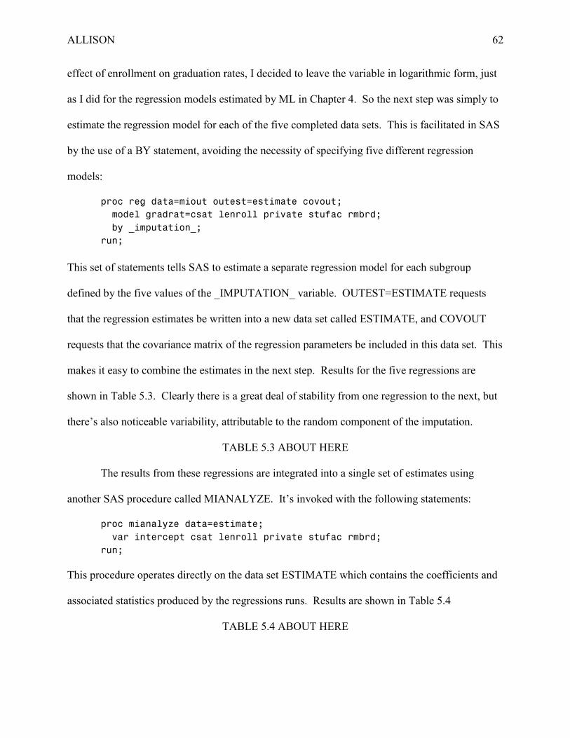
ALLISON 62

effect of enrollment on graduation rates, I decided to leave the variable in logarithmic form, just

as I did for the regression models estimated by ML in Chapter 4. So the next step was simply to

estimate the regression model for each of the five completed data sets. This is facilitated in SAS

by the use of a BY statement, avoiding the necessity of specifying five different regression

models:

proc reg data=miout outest=estimate covout; model gradrat=csat lenroll private stufac rmbrd; by _imputation_;run;

This set of statements tells SAS to estimate a separate regression model for each subgroup

defined by the five values of the _IMPUTATION_ variable. OUTEST=ESTIMATE requests

that the regression estimates be written into a new data set called ESTIMATE, and COVOUT

requests that the covariance matrix of the regression parameters be included in this data set. This

makes it easy to combine the estimates in the next step. Results for the five regressions are

shown in Table 5.3. Clearly there is a great deal of stability from one regression to the next, but

there’s also noticeable variability, attributable to the random component of the imputation.


The results from these regressions are integrated into a single set of estimates using

another SAS procedure called MIANALYZE. It’s invoked with the following statements:

proc mianalyze data=estimate; var intercept csat lenroll private stufac rmbrd;run;

This procedure operates directly on the data set ESTIMATE which contains the coefficients and

associated statistics produced by the regressions runs. Results are shown in Table 5.4


ALLISON 63

The column labeled “Mean” in Table 5.4 contains the means of the coefficients in Table

5.3. The standard errors, calculated using formula (5.1), are appreciably larger than the standard

errors in Table 5.3. That’s because the between-regression variability is added to the within-

regression variability. But there’s more between-regression variability for some coefficients than

for others. At the low end, the standard error for the LENROLL coefficient in Table 5.4 is only

about 10 percent larger than the mean of the standard errors in Table 5.3. At the high end, the

combined standard error for RMBRD is about 70 percent larger than the mean of the individual

standard errors. The greater variability in the RMBRD coefficients is apparent in Table 5.3

where the estimates range from 1.66 to 2.95.

The column labeled “t for H0: Mean=0” in Table 5.4 is just the ratio of each coefficient

to its standard error. The immediately preceding column gives the degrees of freedom used to

calculate the p-value from a t-table. This number has nothing to do with the number of

observations or the number of variables. It’s simply a way of specifying a reference distribution

that happens to be a good approximation to the sampling distribution of the t-ratio statistic.

Although it’s not essential to know how the degrees of freedom is calculated, I think it’s worth a

short explanation. For a given coefficient, let U be the average of the squared, within-regression

standard errors. Let B be the variance of the coefficients between regressions. The relative

increase in variance due to missing data is defined as

UBMr )1( 1−+=

where M is, as before, the number of completed data sets used to produce the estimates. The

degrees of freedom is then calculated as

( )211)1( −+−= rMdf

ALLISON 64

Thus, the smaller the between-regression variation relative to the within-regression variation, the

larger the degrees of freedom. Sometimes the calculated degrees of freedom will be

substantially greater than the number of observations. That’s nothing to be concerned about

because any number greater than about 150 will yield a t table that is essentially the same as a

standard normal distribution. However, some software (including PROC MI) can produce an

adjusted degrees of freedom that cannot be greater than the sample size (Barnard and Rubin

1999).

The last column, “Fraction Missing Information,” is an estimate of how much

information about each coefficient is lost because of missing data. It ranges from a low of 21

percent for LENROLL to a high of 71 percent for RMBRD. It’s not surprising that the missing

information is high for RMBRD, which had 40 percent missing data, but it’s surprisingly high

for PRIVATE, which had no missing data, and STUFAC, which had less than 1 percent missing

data. To understand this, it’s important to know a couple things. First, the amount of missing

information for a given coefficient depends not only on the missing data for that particular

variable, but also on the percentage of missing data for other variables that are correlated with

the variable. Second, the MIANALYZE procedure has no way of knowing how much missing

data there is on each variable. Instead, the missing information estimate is based entirely on the

relative variation within and between regressions. If there’s a lot of variation between

regressions, that’s an indication of a lot of missing information. Sometimes denoted as γ, the

fraction of missing information is calculated from two statistics that we just defined, r and df.

Specifically,

1)3/(2ˆ

+++=

rdfrγ .

ALLISON 65

Keep in mind that the fraction of missing information reported in the table is only an estimate

that may be subject to considerable sampling variability.

As noted earlier, one of the troubling things about multiple imputation is that it does not

produce a determinate result. Every time you do it, you get slightly different estimates and

associated statistics. To see this, take a look at Table 5.5, which is based on five data sets

produced by an entirely new run of data augmentation. Most of the results are quite similar to

those in Table 5.4, although note that the fractions of missing information for LENROLL and

PRIVATE are much lower than before.


When the fraction of missing information is high, more than the recommended three to

five completed data sets may be necessary to get stable estimates. How many might that be?

Multiple imputation with an infinite number of data sets is fully efficient (like ML), but MI with

a finite number of data sets does not achieve full efficiency. Rubin (1987) showed that the

relative efficiency of an estimate based on M data sets compared with one based on an infinite

number of data sets is given by (1 + γ /M)-1, where γ is the fraction of missing information. This

implies that with 5 data sets and 50 percent missing information, the efficiency of the estimation

procedure is 91 percent. With 10 data sets, the efficiency goes up to 95 percent. Equivalently,

using only five data sets would give us standard errors that are 5 percent larger than using an

infinite number of data sets. Ten data sets would yield standard errors that are 2.5 percent larger

than an infinite number of data sets. The bottom line is that even with 50 percent missing

information, five data sets do a pretty good job. Doubling the number of data sets cuts the excess

standard error in half, but the excess is small to begin with.

ALLISON 66

Before leaving the regression example, let’s compare the MI results in Table 5.5 with the

ML results in Table 4.6. The coefficient estimates are quite similar, as are the standard errors

and t-statistics. Certainly one would reach the same conclusions from the two analyses.

ALLISON 67

Table 5.1. Correlations and Standard Errors for Randomly Imputed Data.

Correlation S.E.

.3159 .00900

.3108 .00903

.3135 .00902

.3210 .00897

.3118 .00903

.3022 .00909

.3189 .00898

.3059 .00906

ALLISON 68

Table 5.2. Correlations and Standard Errors for Randomly Imputed Data Using the Data

Augmentation Method

Correlation S.E.

0.30636 .0090614

0.31316 .0090193

0.31837 .0089864

0.31142 .0090302

0.32086 .0089705

0.29760 .0091143

0.32701 .0089306

0.30826 .0090498

ALLISON 69

Table 5.3 Regression Coefficients (and Standard Errors) for Five Completed Data Sets

Intercept -33.219 (4.272) -33.230 (4.250) -31.256 (4.306) -34.727 (4.869) -29.117 (4.924)

CSAT 0.069 (0.004) 0.067 (0.004) 0.071 (0.004) 0.069 (0.004) 0.065 (0.004)

LENROLL 1.550 (0.534) 2.023 (0.526) 1.852 (0.546) 2.187 (0.532) 1.971 (0.538)

PRIVATE 11.632 (1.124) 12.840 (1.126) 12.274 (1.157) 13.468 (1.121) 12.191 (1.141)

STUFAC -0.145 (0.083) -0.116 (0.082) -0.213 (0.084) -0.142 (0.083) -0.231 (0.084)

RMBRD 2.951 (0.390) 2.417 (0.392) 1.657 (0.408) 2.103 (0.391) 2.612 (0.393)

ALLISON 70

Table 5.4 Selected Output from PROC MIANALYZE.

Multiple-Imputation Parameter Estimates

Fraction

Std Error t for H0: Missing

Variable Mean Mean DF Mean= 0 Pr > |t| Information

intercept -32.309795 5.639411 72 -6.596995 <.0001 0.255724

csat 0.068255 0.004692 39 14.547388 <.0001 0.356451

lenroll 1.916654 0.595229 110 3.220027 0.0017 0.206210

private 12.481050 1.367858 40 9.124524 <.0001 0.344151

stufac -0.169484 0.099331 42 -1.706258 0.0953 0.329284

rmbrd 2.348136 0.670105 10 3.504132 0.0067 0.708476

ALLISON 71

Table 5.5 Output from MIANALYZE for Replication of Multiple Imputation

Multiple-Imputation Parameter Estimates Fraction

Std Error t for H0: Missing

Variable Mean Mean DF Mean=0 Pr > |t| Information

intercept -32.474158 4.816341 124 -6.742496 <.0001 0.192429

csat 0.066590 0.005187 20 12.838386 <.0001 0.489341

lenroll 2.173214 0.546177 2157 3.978955 <.0001 0.043949

private 13.125024 1.171488 1191 11.203719 <.0001 0.059531

stufac -0.190031 0.099027 51 -1.918988 0.0607 0.307569

rmbrd 2.357444 0.599341 12 3.933396 0.0020 0.623224

ALLISON 72

Figure 5.1 Estimates of Regression Slope of GRADRAT on CSAT for the First 100Iterations of Data Augmentation.

Csat _B

0. 084

0. 085

0. 086

0. 087

0. 088

0. 089

0. 090

0. 091

0. 092

0. 093

0. 094

0. 095

0. 096

0. 097

0. 098

I t erat i on

0 10 20 30 40 50 60 70 80 90 100

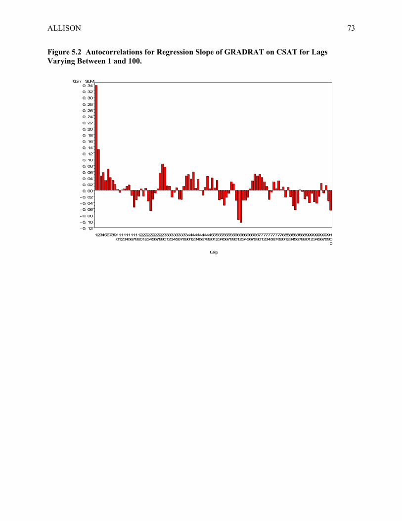
ALLISON 73

Figure 5.2 Autocorrelations for Regression Slope of GRADRAT on CSAT for LagsVarying Between 1 and 100.

Corr SUM

-0. 12

-0. 10

-0. 08

-0. 06

-0. 04

-0. 02

0. 00

0. 02

0. 04

0. 06

0. 08

0. 10

0. 12

0. 14

0. 16

0. 18

0. 20

0. 22

0. 24

0. 26

0. 28

0. 30

0. 32

0. 34

Lag

123456789101112131415161718192021222324252627282930313233343536373839404142434445464748495051525354555657585960616263646566676869707172737475767778798081828384858687888990919293949596979899100

ALLISON 74

6. MULTIPLE IMPUTATION: COMPLICATIONS

Interactions and Nonlinearities in MI

While the methods we have just described are very good for estimating the main effects

of the variables with missing data, they may not be so good for estimating interaction effects.

Suppose, for example, we suspect that the effect of SAT scores (CSAT) on graduation rate

(GRADRAT) is different for public and private colleges. One way to test this hypothesis

(Method 1) would be to take the previously imputed data, create a new variable which is the

product of CSAT and PRIVATE, and include this product term in the regression equation along

with the other variables already in the model. The leftmost panel of Table 6.1 (Method 1) shows

the results of doing this. The variable PRIVCSAT is the product of CSAT and PRIVATE. With

a p-value of .39, the interaction is far from statistically significant. So we would conclude that

the effect of CSAT does not vary between public and private institutions.


The problem with this approach is that while the multivariate normal model is good at

imputing values that reproduce the linear relationships among variables, it does not model any

higher-order moments. Consequently, the imputed values will not display any evidence of

interaction unless special techniques are implemented. In this example, where one of the two

variables in the interaction is a dichotomy (PRIVATE), the most natural solution (Method 2) is

to do separate chains of data augmentation for private colleges and for public colleges. This

allows the relationship between CSAT and GRADRAT to differ across the two groups, and for

the imputed values to reflect that fact. Once the separate imputations are completed, the data sets

are re-combined into a single data set, the product variable is created, and the regression is run

with the product variable. Results in the middle panel of Table 6.1 shows that the interaction

ALLISON 75

between PRIVATE and CSAT is significant at the .02 level. More specifically, we find that the

positive effect of CSAT on graduation rates is smaller in private colleges than in public colleges.

A third approach (Method 3) is to create the product variable for all cases with observed

values of CSAT and PRIVATE before imputation. Then impute the product variable just like

any other variable with missing data. Finally, using the imputed data, estimate the regression

model that includes the product variable. This method is less appealing than Method 2 because

the product variable will typically have a distribution that is far from normal, yet normality is

assumed in the imputation process. Nevertheless, as seen in the right-hand panel of Table 6.1,

the results from Method 3 are very close to those obtained with Method 2, certainly much closer

than those of Method 1.

The results for Method 3 are reassuring because Method 2 is not feasible when both

variables in the interaction are measured on quantitative scales. Thus, if we wish to estimate a

model with the interaction of CSAT and RMBRD, we need to create a product variable for the

476 cases that have data on both these variables. For the remaining 826 cases, we must impute

the product term as part of the data augmentation process. This method (or Method 2 when

possible) should be used whenever the goal is to estimate a model with nonlinear relationships

involving variables with missing data. For example, if we want to estimate a model with both

RMBRD and RMBRD squared, the squared term should be imputed as part of the data

augmentation. This requirement puts some burden on the imputer to anticipate the desired

functional form before beginning the imputation. It also means that one must be cautious about

estimating nonlinear models from data that have been imputed by others using strictly linear

models. Of course, if the percentage of missing data on a given variable is small, one may be

able to get by with imputing a variable in its original form and then constructing a nonlinear

ALLISON 76

transformation later. Certainly for the variable STUFAC (student/faculty ratio), with only two

cases missing out of 1302, it would be quite acceptable to put STUFAC squared in a regression

model after simply squaring the two imputed values rather than imputing the squared values.

Compatibility of the Imputation Model and the Analysis Model

The problem of interactions illustrates a more general issue in multiple imputation.

Ideally, the model used for imputation should agree with the model used in analysis, and both

should correctly represent the data. The basic formula (5.1) for computing standard errors

depends on this compatibility and correctness.

What happens when the imputation and analysis models differ? That depends on the

nature of the difference and which model is correct (Schafer 1997). Of particular interest are

cases in which one model is a special case of the other. For example, the imputation model may

allow for interactions but the analysis model may not. Or the analysis model may allow for

interactions but the imputation model may not. In either case, if the additional restrictions

imposed by the simpler model are correct, then the procedures we have discussed for inference

under multiple imputation will be valid. But if the additional restrictions are not correct,

inferences using the standard methods may not be valid.

Methods have been proposed for estimating standard errors under multiple imputation

that are less sensitive to the model choice (Wang and Robins 1998, Robins and Wang 2000).

Specifically, these methods give valid standard error estimates when the imputation and analysis

models are incompatible, and when both models are incorrect. Nevertheless, incorrect models at

either stage may still give biased parameter estimates. And the alternative methods require

specialized software that is not yet readily available.

ALLISON 77

Role of the Dependent Variable in Imputation

Because GRADRAT was one of the variables included in the data augmentation process,

the dependent variable was implicitly used to impute missing values on the independent

variables. Is this legitimate? Doesn’t it tend to produce spuriously large regression coefficients?

The answer is that not only is this OK, it is essential for getting unbiased estimates of the

regression coefficients. With deterministic imputation, using the dependent variable to impute

the missing values of the independent variables can, indeed, produce spuriously large regression

coefficients. But the introduction of a random component into the imputation process

counterbalances this tendency and gives us approximately unbiased estimates. In fact, leaving

the dependent variable out of the imputation process tends to produce regression coefficients that

are spuriously small, at least for those variables that have missing data (Landerman et al. 1997).

In the college example, if GRADRAT is not used in the imputations, the coefficients for CSAT

and RMBRD, both with large fractions of missing data, are reduced by about 25 percent and 20

percent, respectively. At the same time, the coefficient for LENROLL, which only had five

missing values, is 65 percent larger.

Of course, including GRADRAT in the data augmentation process also means that any

missing values of GRADRAT were also imputed. Some authors have recommended against

imputing missing data on the dependent variable (Cohen and Cohen 1985). To follow this

advice we would have to delete any cases with missing data on the dependent variable before

beginning the imputation. There is a valid rationale for this recommendation, but it applies only

in special cases. If there is missing data on the dependent variable but not on any of the

independent variables, maximum likelihood estimation of a regression model (whether linear or

nonlinear) does not use any information from cases with missing data. Since ML is optimal,

ALLISON 78

there is nothing to gain from imputing the missing cases under multiple imputation. In fact,

although such imputation wouldn’t lead to any bias, the standard errors would be larger.

However, the situation changes when there is also missing data on the independent variables.

Then cases with missing values on the dependent variables do have some information to

contribute to the estimation of the regression coefficients, although probably not a great deal.

The upshot is that in the typical case with missing values on both dependent and independent

variables, the cases with missing values on the dependent variable should not be deleted.

Using Additional Variables in the Imputation Process

As already noted, the set of variables used in data augmentation should certainly include

all variables that will be used in the planned analysis. In the college example, we also included

one additional variable ACT (mean ACT scores) because of its high correlation with CSAT, a

variable with substantial missing data. The goal was to improve the imputations of CSAT in

order to get more reliable estimates of its regression coefficient. We might have done even better

had we included still other variables that were correlated with CSAT.

Here’s a somewhat simpler example that illustrates the benefits of additional predictor

variables. Suppose we want to estimate the mean CSAT score across the 1302 colleges. As we

know, data are missing on CSAT for 523 cases. If we calculate the mean for the other 779 cases

with values on CSAT, we get the results in the first line of Table 5.7. The next line shows the

estimated mean (with standard error) using multiple imputation and the ACT variable. The mean

has decreased by 9 points while the standard error has decreased by 13 percent. Although ACT

has a correlation of about .90 with CSAT, its usefulness as a predictor variable is somewhat

marred by the fact that values are observed on ACT for only 226 of the 523 cases missing on

CSAT. If we add an additional variable, PCT25 (the percentage of students in the top 25 percent

ALLISON 79

of their class) we get an additional reduction in standard error. PCT25 has a correlation of about

.80 with CSAT and is available for an additional 240 cases that have missing data on both CSAT

and ACT.

The last line of Table 6.2 adds in GRADRAT, which has a correlation of about .60 with

CSAT but is only available for 17 cases not already covered by PCT25 or ACT. Not

surprisingly, the decline in the standard error is quite small. When I tried introducing all the

other variables in the regression model in Table 5.5, the standard error actually got larger. This

is likely due to the fact that the other variables have much lower correlations with CSAT, yet

additional variability is introduced because of the need to estimate their regression coefficients

for predicting CSAT. As in other forecasting problems, imputations may get worse when poor

predictors are added to the model.


Other Parametric Approaches to Multiple Imputation

As we have seen, multiple imputation under the multivariate normal model is reasonably

straightforward under a wide variety of data types and missing data patterns. As a routine

method for handling missing data, it’s probably the best that is currently available. There are,

however, several alternative approaches that may be preferable in some circumstances.

One of the most obvious limitations of the multivariate normal model is that it’s only

designed to impute missing values for quantitative variables. As we’ve seen, categorical

variables can be accommodated by using some ad hoc fix-ups. But sometimes you may want to

do better. For situations in which all variables in the imputation process are categorical, a more

attractive model is the unrestricted multinomial model (which has a parameter for every cell in

the contingency table) or a loglinear model that allows restrictions on the multinomial

ALLISON 80

parameters. In Chapter 4, we discussed ML estimation of these models. Schafer (1997) has

shown how these models can also be used as the basis for data augmentation to produce multiple

imputations, and he has developed a freeware program called CAT to implement the method

(http://www.stat.psu.edu/~jls/).

Another Schafer program (MIX) uses data augmentation to generate imputations when

the data consists of a mixture of categorical and quantitative variables. The method presumes

that the categorical variables have a multinomial distribution, possibly with loglinear restrictions

on the parameters. Within each cell of the contingency table created by the categorical variables,

it is assumed that the quantitative variables have a multivariate normal distribution. The means

of these variables are allowed to vary across cells, but the covariance matrix is assumed to be

constant.

At this writing, both CAT and MIX are only available as libraries to the S-Plus statistical

package, although stand-alone versions are promised. In both cases, the underlying models

potentially have many more parameters than the multivariate normal model. As a result,

effective use of these methods typically requires more knowledge and input from the person

performing the imputation, together with larger sample sizes to achieve stable estimates.

If data are missing for a single categorical variable, multiple imputation under a logistic

(logit) regression model is reasonably straightforward (Rubin 1987). Suppose data are missing

on marital status, coded into five categories, and there are several potential predictor variables,

both continuous and categorical. For purposes of imputation, we estimate a multinomial logit

model for marital status as a function of the predictors, using cases with complete data. This

produces a set of coefficient estimates β̂ and an estimate of the covariance matrix )ˆ(ˆ βV . To

allow for variability in the parameter estimates, we take a random draw from a normal

ALLISON 81

distribution with a mean of β̂ and a covariance matrix )ˆ(ˆ βV . (Schafer (1997) has practical

suggestions on how to do this efficiently). For each case with missing data, the drawn coefficient

values and the observed covariate values are substituted into the multinomial logit model to

generate predicted probabilities of falling into the five marital status categories. Based on these

predicted probabilities, we randomly draw one of the marital status categories as the final

imputed value.11 The whole process is repeated multiple times to generate multiple completed

data sets. Of course, a binary variable would be just a special case of this method. This

approach can also be used with a variety of other parametric models, including Poisson

regression and parametric failure-time regressions.

Non-Parametric and Partially Parametric Methods

Many methods have been proposed for doing multiple imputation under less stringent

assumptions than the fully parametric methods we have just considered. In this section, I’ll

consider a few representative approaches, but keep in mind that each of these has many different

variations. All these methods are most naturally applied when there is missing data on only a

single variable, although they can often be generalized without difficulty to multiple variables

when data are missing in a monotone pattern (described in Chapter 4). See Rubin (1987) for

details on the monotone generalizations. These methods can sometimes be used when the

missing data do not follow a monotone pattern, but in such settings they typically lack solid

theoretical justification.

In choosing between parametric and nonparametric methods, there is the usual trade-off

between bias and sampling variability. Parametric methods tend to have less sampling

variability, but they may give biased estimates if the parametric model is not a good

ALLISON 82

approximation to the phenomenon of interest. Nonparametric methods may be less prone to bias

under a variety of situations, but the estimates often have more sampling variability.

Hot Deck Methods

The best-known approach to nonparametric imputation is the “hot deck” method,

frequently used by the U.S. Census Bureau to produce imputed values for public-use data sets.

Here’s the basic idea. We want to impute missing values for a particular variable Y, which may

be either quantitative or categorical. We find a set of categorical X variables (with no missing

data) that are associated with Y. We form a contingency table based on the X variables. If there

are cases with missing Y values within a particular cell of the contingency table, we take one or

more of the nonmissing cases in the same cell and use their Y values to impute the missing Y

values.

Obviously there are a lot of complications that may arise. The critical question is how do

you choose which “donor” values to assign to the cases with missing values? Clearly the choice

of donor cases should somehow be randomized to avoid bias. This leads naturally to multiple

imputation since any randomized method can be applied more than once to produce different

imputed values. The trick is to do the randomization in such a way that all the natural variability

is preserved. To accomplish this, Rubin proposed a method he coined the approximate Bayesian

bootstrap (ABB) (Rubin 1987, Rubin and Schenker 1991). Here’s how it’s done. Suppose that

in a particular cell of the contingency table, there are n1 cases with complete data on Y and n0

cases with missing data on Y. Follow these steps:

1. From the set of n1 cases with complete data, take a random sample (with replacement)

of n1 cases.

2. From this sample, take a random sample (with replacement) of n0 cases.

ALLISON 83

3. Assign the n0 observed values of Y to the n0 cases with missing data on Y.

4. Repeat steps 1-3 for every cell in the contingency table.

These four steps produce one completed data set when applied to all cells of the contingency

table. For multiple imputation, the whole process is repeated multiple times. After the desired

analysis is performed on each data set, the results are combined using the same formulas we used

for the multivariate normal imputations.

While it might seem that one could skip step 1 and directly choose n0 donor cases from

among the n1 cases with complete data, this does not produce sufficient variability for estimating

standard errors. Additional variability comes from the fact that sampling in step 2 is with

replacement.

Predictive Mean Matching

A major attraction of hot deck imputation is that the imputed values are all actual

observed values. Consequently, there are no “impossible” or out-of-range values, and the shape

of the distribution tends to be preserved. A disadvantage is that the predictor variables must all

be categorical (or treated as such), imposing serious limitations on the number of possible

predictor variables. To remove this limitation, Little (1988) proposed a partially parametric

method called predictive mean matching. Like the multivariate normal parametric method, this

approach begins by regressing Y, the variable to be imputed, on a set of predictors for cases with

complete data. This regression is then used to generate predicted values for both the missing and

nonmissing cases. Then, for each case with missing data, we find a set of cases with complete

data that have predicted values of Y that are “close” to the predicted value for the case with

missing data. From this set of cases, we randomly choose one case whose Y value is donated to

the missing case.

ALLISON 84

For a single Y variable, it’s straightforward to define closeness as the absolute difference

between predicted values. But then one must decide how many of the close predicted values to

include in the donor pool for each missing case. Or, equivalently, what should be the cut-off

point in closeness for forming the set of possible donor values? If a small donor pool is chosen,

there will be more sampling variability in the estimates. On the other hand, too large a donor

pool can lead to possible bias because many donors may be unlike the recipients. To deal with

this ambiguity, Schenker and Taylor (1991) developed an “adaptive method” that varies the size

of the donor pool for each missing case, based on the “density” of complete cases with close

predicted values. They found that their method did somewhat better than methods with fixed

size donor pools of either 3 or 10 closest cases. But the differences among the three methods

were sufficiently small that the adaptive method hardly seems worth the extra computational

cost.

In doing predictive mean matching, it’s also important to adjust for the fact that the

regression coefficients are only estimates of the true coefficients. As in the parametric case, this

can be accomplished by randomly drawing a new set of regression parameters from their

posterior distribution before calculating predicted values for each imputed data set. Here’s how

to do it:

1. Regress Y on X (a vector of covariates) for the n1 cases with no missing data on y,

producing regression coefficients b (a k × 1 vector) and residual variance estimate s2.

2. Make a random draw from the posterior distribution of the residual variance

(assuming a noninformative prior). This is accomplished by calculating (n1-k) s2/χ2,

where χ2 represents a random draw from a chi-square distribution with n1-k degrees

of freedom. Let s2[1] be the first such random draw.

ALLISON 85

3. Make a random draw from the posterior distribution of the regression coefficients.

This is accomplished by drawing from a multivariate normal distribution with mean b

and covariance matrix s2[1](X’X)-1 where X is an n1 × k matrix of X values. Let b[1] be

the first such random draw. See Schafer (1997) for practical suggestions on how to

do this.

For each new set of regression parameters, predicted values are generated for all cases.

Then, for each case with missing data on Y, we form a donor pool based on the predicted values,

and randomly choose one of the observed values of Y from the donor pool. This approach to

predictive mean matching can be generalized to more than one Y variable with missing data,

although the computations may become rather complex (Little 1988).

Sampling on Empirical Residuals

In the data augmentation method, residual values are sampled from a standard normal

distribution and then added to the predicted regression values to get the final imputed values.

We can modify this method to be less dependent on parametric assumptions by making random

draws from the actual set of residuals produced by the linear regression. This can yield imputed

values whose distribution is more like that of the observed variable (Rubin 1987), although it’s

still possible to get imputed values that are outside the permissible range.

As with other approaches to multiple imputation, there are some important subtleties

involved in doing this properly. As before, let Y be the variable with missing data to be imputed

for n0 cases, and with observed data on n1 cases. Let X be a k × 1 vector of variables (including a

constant) with no missing data on the n1 cases. We begin by performing the three steps given

immediately above to obtain the linear regression of Y on X and generate random draws from the

posterior distribution of the parameters. Then we add the following steps:

ALLISON 86

4. Based on the regression estimates in step 1, calculate standardized residuals for the

cases with no missing data:

snkbxye iii /)/1)(( 1−−= .

5. Draw a simple random sample (with replacement) of n0 values from the n1 residuals

calculated in step 4.

6. For the n0 cases with missing data, calculate imputed values of Y as

iii esxby ]1[]1[ +=

where ei represents the residuals drawn in step 4, and b[1] and s[1] are the first random

draws from the posterior distribution of the parameters.

These six steps produce one completed set of data. To get additional data sets, simply

repeat steps 2 through 6 (except for step 4 which should not be repeated).

As Rubin (1987) explains, this methodology can be readily extended to data sets with a

monotonic missing pattern on several variables. Each variable is imputed using as predictors all

variables that are observed when it is missing. The empirical residual method can also be

modified to allow for heteroscedasticity in the imputed values (Schenker and Taylor 1996). For

each case to be imputed, the pool of residuals is restricted to those observed cases that have

predicted values of Y that are close to the predicted value for the case with missing data.

Example

Let’s try the partially parametric methods on a subset of the college data. TUITION is

fully observed for 1,272 colleges. (For simplicity, we shall exclude the 30 cases with missing

data on this variable.) Of these 1,272 colleges, only 796 report BOARD, the annual average cost

of board at each college. Using TUITION as a predictor, our goal is to impute the missing

ALLISON 87

values of BOARD for the other 476 colleges, and estimate the mean of BOARD for all 1,272

colleges.

First, let’s apply the methods we’ve used before. For the 796 colleges with complete data

(listwise deletion), the average BOARD is $2060 with a standard error of 23.4. Applying the

EM algorithm to TUITION and BOARD, we get a mean BOARD of 2032 (but no standard

error). The EM estimate of the correlation between BOARD and TUITION was .555. Multiple

imputation under the multivariate normal model using data augmentation gave a mean BOARD

of 2040 with an estimated standard error of 21.2.

Because BOARD is highly skewed to the right, there is reason to suspect that the

multivariate normal model may not be appropriate. Quite a few of the values imputed by data

augmentation were less than the minimum observed value of 531, and one imputed value was

negative. Perhaps we can do better by sampling on the empirical residuals. For the 796 cases

with data on both TUITION and BOARD, the OLS regression of BOARD on TUITION was

BOARD= 1497.4 + 67.65*TUITION/1000

with a root mean squared error estimated at 542.6. Standardized residuals from this regression

were calculated for the 796 cases.

The estimated regression parameters were used to make five random draws from the

posterior distribution of the parameters as in steps 2 and 3 above (assuming a noninformative

prior). The drawn values were

intercept slope rmse1536.40 66.6509 531.9901503.65 71.5916 552.7081501.61 66.9756 554.8001486.84 66.9850 548.4001504.23 61.2308 534.895

ALLISON 88

To create the first completed data set, 476 residual values were randomly drawn with

replacement from among the 796 cases. These standardized residuals were assigned arbitrarily

to the 476 cases with missing data on BOARD. Letting E be the assigned residual for a given

case, the imputed values for BOARD were generated as

BOARD = 1536.40 + 66.6509*TUITION/1000 + 531.990*E.

This process was repeated for the four remaining data sets, with new sampling on the residuals

and new values of the regression parameters at each step.

Once the five data sets were produced, the mean and standard error were computed for

each data set, and the results combined, using formula (5.1) for the standard error. The final

estimate for the mean of BOARD was 2035 with an estimated standard error of 20.4, which is

quite close to multiple imputation based on a normal distribution.

Now let’s try predictive mean matching. Based on the coefficients from the OLS

regression of BOARD on TUITION, I generated five new random draws from the posterior

distribution of the regression parameters:

intercept slope rmse1465.89 67.8732 557.5311548.98 64.5723 539.9521428.82 67.3901 512.3811469.34 67.3750 550.9451517.92 66.1926 534.804

For the first set of parameter values, I generated predicted values of BOARD for all cases, both

observed and missing. For each case with missing data on BOARD, I found the five observed

cases whose predicted values were closest to the predicted value for the case with missing data. I

randomly chose one of those five cases, and assigned its observed value of BOARD as the

imputed value for the missing case. This process was repeated for each of the five sets of

parameter values, to produce five complete data sets. (It’s just coincidence that the number of

ALLISON 89

data sets is the same as the number of observed cases matched to each missing case). The mean

and standard error were then computed for each data set, and the results were combined in the

usual way. The combined mean of BOARD was 2028 with an estimated standard error of 23.0.

All four imputation methods produced similar estimates of the means, and all were

noticeably lower than the mean based on listwise deletion. Schenker and Taylor (1996) suggest

that while parametric and partially parametric imputation methods tend to yield quite similar

estimates of mean structures (including regression coefficients), they may produce more

divergent results for the marginal distribution of the imputed variables. Their simulations

indicated that for applications where the marginal distribution is of major interest, partially

parametric models have a distinct advantage. This was especially true when the regressions used

to generate predicted values were misspecified in various ways.

Sequential Generalized Regression Models

One of the attractions of data augmentation is that, unlike the nonparametric and

semiparametric methods just discussed, it can easily handle data sets with a substantial number

of variables with missing data. Unfortunately, this method requires specifying a multivariate

distribution for all the variables, and that’s not an easy thing to do when the variables are of

many different types, for example, continuous, binary and count data. Recently, another

approach has been proposed for handling missing data in large, complex data sets with several

different variable types. Instead of fitting a single comprehensive model (e.g., the multivariate

normal), a separate regression model is specified for each variable that has any missing data. For

each dependent variable, the regression model is chosen to reflect the type of data. The method

involves cycling through the several regression models, imputing missing values at each step.

ALLISON 90

While this approach is very appealing, it does not yet have as strong a theoretical

justification as the other methods we have considered. At this writing, the only detailed accounts

are the unpublished reports of Brand (1999), Van Buuren and Oudshoorn (1999) and

Raghunathan, Lepkowski, Van Hoewyk and Solenberger (1999). In Raghunathan’s et al.’s

version of the method, the available models include normal linear regression, binary logistic

regression, multinomial logit, and Poisson regression. The regression models are estimated in a

particular order, beginning with the dependent variable with the least missing data and

proceeding to the dependent variable with the most missing data. Let’s denote these variables by

Y1 through Yk, and let X denote the set of variables with no missing data.

The first “round” of estimation proceeds as follows. Regress Y1 on X and generate

imputed values using a method similar to that described above for the multinomial logit model in

the section “Other Parametric Approaches to Multiple Imputation.” Bounds and restrictions may

be placed on the imputed values. Then regress Y2 on X and Y1, including the imputed values of

Y1, and generate imputed values for Y2. Then regress Y3 on X, Y1 and Y2 (including imputed

values on both Y’s). Continue until all the regressions have been estimated. The second and

subsequent rounds repeat this process, except that now each variable is regressed on all other

variables using any imputed values from previous steps. The process continues for a pre-

specified number of rounds or until stable imputed values occur. A SAS macro for

accomplishing these tasks is available at http://www.isr.umich.edu/src/smp/ive.

For their version of the method, Van Buuren and Oudshoorn have coined the name MICE

(for multiple imputation by chained equations), and they have developed S-PLUS functions to

implement it (available at http://www.multiple-imputation.com/). The major differences

between their approach and that of Raghunathan et al. is that MICE does not include Poisson

ALLISON 91

regression but does allow more options (both parametric and partially parametric) in the methods

for random draws of imputed values.

Linear Hypothesis Tests and Likelihood Ratio Tests

To this point, our approach to statistical inference with multiple imputation has been very

simple. For a given parameter, the standard error of the estimate is calculated using formula

(5.1). This standard error is then plugged into conventional formulas based on the normal

approximation to produce a confidence interval or a t-statistic for some hypothesis of interest.

Sometimes that’s not enough. Often we want to test hypotheses about sets of parameters, for

example, that two parameters are equal to each other, or that several parameters are all equal to

zero. These sorts of hypotheses are particularly relevant when we estimate several coefficients

for a set of dummy variables. In addition, there is often a need to compute likelihood ratio

statistics comparing one model with another, simpler model. Accomplishing these tasks is not

so straightforward when doing multiple imputation. Schafer (1997) describes three different

approaches, none of which is totally satisfactory. I’ll briefly describe them here, and we’ll look

at an example in the next section.

Wald Tests Using Combined Covariance Matrices

When there are no missing data, a common approach to multiple parameter inference is

to compute Wald chi-square statistics based on the parameter estimates and their estimated

covariance matrix. Here’s a review which, unfortunately, requires matrix algebra. Suppose we

we want to estimate a p × 1 parameter vector β . We have estimates β̂ , and estimated

covariance matrix C. We want to test a linear hypothesis expressed as cLβ = where L is an r ×

p matrix of constants and c is an r × 1 vector of constants. For example, if we want to test the

ALLISON 92

hypothesis that the first two elements of β are equal to each other, we need L = [1 -1 0 0 0…0]

and c = 0. The Wald test is computed as

)ˆ(][)ˆ( 1 cβLLLCcβL −′′−= −W (6.1)

which has an approximate chi-square distribution with r degrees of freedom under the null

hypothesis.12

Now let’s generalize this method to the multiple imputation setting. Instead of β̂we can

use β , the mean of the estimates across the several completed data sets. That is,

�=k

kMββ ˆ1

Next we need an estimate of the covariance matrix that combines the within-sample variability

and the between-sample variability. Let Ck be the estimated covariance matrix for the

parameters in data set k, and let C be the average of those matrices across the M data sets. The

between-sample variability is defined as

� ′−−=k

kkM)ˆ)(ˆ(1 ββββB

The combined estimate of the covariance matrix is then

BCC )/11(~ M++=

which is just a multivariate generalization of formula (5.1), without the square root. We get our

test statistic by formula (6.1) with β and C~ substituted for β̂ and C.

Unfortunately, this does not work well in the typical case where M is five or less. In such

cases, B is a rather unstable estimate of the between-sample covariance, and the resulting

distribution of W is not chi-square. Schafer (1997) gives a more stable estimator for the

covariance matrix, but this requires the unreasonable assumption that the fraction of missing

ALLISON 93

information is the same for all the elements of β̂ . Nevertheless, some simulations show that this

alternate method works well even when the assumption is violated. This method has been

incorporated into the SAS procedure MIANALYZE.

Likelihood Ratio Tests

If the model of interest is estimated by maximum likelihood and there are no missing

data, multi-parameter tests are often performed by computing likelihood ratio chi-squares. The

procedure is quite simple. Let l0 be the log-likelihood for a model that imposes the hypothesis,

and l1 be the log-likelihood for a model that relaxes the hypothesis. The likelihood ratio statistic

is just L = 2(l1 – l0).

As before, our goal is to generalize this to multiple imputation. The first step is to

perform the desired likelihood ratio test in each of the M completed data sets. Let L be the

mean of the likelihood ratio chi-squares computed across those M data sets. That’s the easy part.

Now comes the hard part. To get those chi-squares, it was necessary to estimate two models in

each data set, one with the hypothesis imposed and one with the hypothesis relaxed. Let 0β be

the mean of the M parameter estimates when the hypothesis is imposed, and let 1β be the mean

of the parameter estimates when the hypothesis is relaxed. In each data set, we then compute the

log-likelihood for a model with parameter values forced to be 0β and again for a model with

parameters set at 1β . (This obviously requires that the software be able to calculate and report

log-likelihoods for user-specified parameter values). Based on these two log-likelihoods, a

likelihood ratio chi-square is computed in each data set. Let L~ be the mean of these chi-square

statistics across the M samples.

The final test statistic is then

ALLISON 94

( )LLr

L

MM ~

~

1

1 −��

��

�+−

+

where r is the number of restrictions imposed by the hypothesis. Under the null hypothesis, this

statistic has approximately an F distribution with numerator degrees of freedom equal to r. The

denominator degrees of freedom (d.d.f) is somewhat awkward to calculate. Let t=r(M-1) and let

��

��

� −��

��

�=−

+

rLLq

M

M~

1

1 .

If t > 4, the d.d.f. is 2]/)/21(1)[4(4 qtt −+−+ . If t ≤ 4, the d.d.f. is t(1+1/k)(1+1/q)2/2.

Combining Chi-Square Statistics

Both the Wald test and the likelihood ratio test lack the appealing simplicity of the single-

parameter methods used earlier. In particular, they require that the analysis software have

specialized options and output, something we have generally tried to avoid. I now discuss a third

method that is easy to compute from standard output, but may not be as accurate as the other two

methods (Li et al. 1991). All that’s needed is the conventional chi-square statistic (either Wald

or likelihood ratio) calculated in each of the M completed data sets, and the associated degrees of

freedom.

Let dk2 be a chi-square statistic with r degrees of freedom calculated in data set k. Let 2d

be the mean of these statistics over the M data sets, and let 2ds be the sample variance of the

square roots of the chi-square statistics over the M data sets. That is,

� −−

=k

kd ddM

s 22 )(1

1 .

The proposed test statistic is

ALLISON 95

2

22

)/11(1)/11(/

d

d

sMsMrdD

++−−= .

Under the null hypothesis, this statistic has approximately an F distribution with r as the

numerator degrees of freedom. The denominator degrees of freedom is approximated by

��

��

�

++�

�

��

� −2/3 )/11(

111

dM sMk

M

I have written a SAS macro (COMBCHI) to perform these computations and compute a p-value.

It is available on my web site (http://www.ssc.upenn.edu/~allison). To use it, all you need to do

is enter several chi-square values and the degrees of freedom. The macro returns a p-value.

MI Example 2

Let’s consider another detailed empirical example that illustrates some of the techniques

discussed in this chapter. The data set consists of 2,992 respondents to the 1994 General Social

Survey (Davis and Smith 1997). Our dependent variable is SPANKING, a response to the

question “Do you strongly agree, disagree, or strongly disagree that it is sometimes necessary to

discipline a child with a good, hard spanking?” As the question itself indicates, there were four

possible ordered responses, coded as integers 1 through 4. By design, this question was part of a

module that was only administered to a random two-thirds of the sample. Thus, there were 1,015

cases that were missing completely at random. In addition, another 27 respondents were missing

with responses coded “don’t know” or “no answer”.

Our goal is to estimate an ordered logistic (cumulative logit) model (McCullagh 1980) in

which SPANKING is predicted by the following variables:

AGE Respondent’s age in years, ranging from 18 to 89. Missing 6 cases.

EDUC Number of years of schooling. Missing 7 cases.

ALLISON 96

INCOME Household income, coded as the midpoint of 21 interval categories, in thousands

of dollars. Missing 356 cases.

FEMALE 1= female, 0=male.

BLACK 1=black, 0=white, other.

MARITAL 5 categories of marital status. Missing 1 case.

REGION 9 categories of region.

NOCHILD 1=no children, otherwise 0. Missing 9 cases.

One additional variable, NODOUBT, requires further explanation. Respondents were

asked about their beliefs in God. There were six response categories ranging from “I don’t

believe in God” to “I know God really exists and I have no doubts about it.” The latter statement

was the modal response, with 62 percent of the respondents. However, like the spanking

question, this question was part of a module that was only asked of a random subset of 1386

respondents. So there were 1606 cases missing by design. Another 60 cases were treated as

missing because they said “don’t know” or “no answer”. As used here, the variable was coded 1

if the respondent had “no doubts”, otherwise 0.

Most of the missing data is on three variables, SPANKING, NODOUBT and INCOME.

There were five major missing data patterns in the sample, accounting for 96 percent of

respondents:

771 cases No missing data on any variables

927 cases Missing NODOUBT only

421 cases Missing SPANKING only

80 cases Missing INCOME only

509 cases Missing SPANKING and NODOUBT

ALLISON 97

160 cases Missing NODOUBT and INCOME

As usual, the simplest approach to data analysis is listwise deletion, which uses only 26

percent of the original sample. In specifying the model, I created dummy variables for three

marital status categories: NEVMAR (for never married), DIVSEP (for divorced or separated),

and WIDOW (for widowed), with married as the reference category. Three dummy variables

were created for region (with West as the omitted category).13 Results (produced by PROC

LOGISTIC in SAS) are shown in the first column of Table 6.3. Blacks, older respondents and

those with “no doubts” about God are more likely to favor spanking. Women and more educated

respondents are more likely to oppose it. There are also major regional differences, with those

from the South more favorable toward spanking and those from the Northeast more opposed. On

the other hand, there is no evidence for any effect of income, marital status, or having children.


Because 84 percent of the observations with missing data are missing by design (and

hence completely at random), listwise deletion should produce approximately unbiased

estimates. But the loss of nearly three quarters of the sample is a big price to pay, one that is

avoidable with multiple imputation. To implement MI, I first used the data augmentation

method under the multivariate normal model, described in Chapter 5. Before beginning the

process, the single case with missing data on marital status was deleted to avoid having to impute

a multi-category variable. A reasonable case could be made for also deleting the 1,042 cases that

were missing the SPANKING variable since cases that are missing on the dependent variable

contain little information about regression coefficients. But there’s no harm in including them

and potentially some benefit, so I kept them in. All 13 variables in the model were included in

the imputation process, without any normalizing transformations.

ALLISON 98

The imputed values for all the dummy variables were rounded to 0 or 1. The imputed

values for SPANKING were rounded to the integers 1 through 4. Age and income had some

imputed values that were out of the valid range, and these were recoded to the upper or lower

bounds. The cumulative logit model was then estimated for each of the five data sets, and the

estimates were combined using the standard formulas.

Results are shown in the second column of Table 6.3. The basic pattern is the same,

although there is a now a significant effect of INCOME and a loss of significance for AGE.

What’s most striking is that the standard errors for all the coefficients are substantially lower

than those for listwise deletion, typically by about 40 percent. Even the standard error for

NODOUBT is 18 percent smaller, which is surprising given that over half the cases were missing

on this variable. The smaller standard errors yield p-values which are much lower for many of

the variables.

The cumulative logit model imposes a constraint on the data known as the “proportional

odds assumption.” In brief, this means that the coefficients are assumed to be the same for any

dichotomization of the dependent variable. PROC LOGISTIC reports a chi-square statistic

(score test) for the null hypothesis that the proportional odds assumption is correct. But since we

are working with five data sets, we get five chi-squares, each with 26 degrees of freedom: 32.0,

31.3, 38.0, 36.4 and 35.2. Using the COMBCHI macro described earlier, these five values are

combined to produce a p-value of .25, suggesting that the constraint imposed by the model fits

the data well. For each of the five data sets, I also calculated Wald chi-squares for the null

hypothesis that all the region coefficients were zero. With 3 d.f., the values were 72.9, 81.3,

53.4, 67.7, and 67.0. The combined p-value was .00002.

ALLISON 99

In the third column of Table 6.3, we see results of applying the multiple imputation

method of Raghunathan et al. (1999) which relies on sequential generalized regressions. A

regression model was estimated for each variable with missing data, taken as the dependent

variable, and all other variables as predictors. These regression models were then used to

generate five sets of random imputations. For EDUC and INCOME, the models were ordinary

linear regression models, although upper and lower bounds were built into the imputation

process. Logistic regression models were specified for NODOUBT and NOCHILD. A

multinomial logit model was used for SPANKING. There were 20 rounds in the imputation

process, which means that for each of the five completed data sets, the variables with missing

data were sequentially imputed 20 times before using the final result.

As before, the cumulative logit model was estimated on each of the five completed data

sets, and the results were combined using the standard formulas. The coefficient estimates in the

third column of Table 6.3 are quite similar to those for multivariate normal data augmentation.

The standard errors are generally a little higher than those for data augmentation, although not

nearly as high as those for listwise deletion.

Somewhat surprising is the fact that the chi-square statistics for the proportional odds

assumption are nearly twice as large for sequential regression as those for normal data

augmentation. Specifically, with 26 degrees of freedom, the values were 54.9, 59.9, 66.7, 85.4,

and 59.0, each with a p-value well below .001. But when they are combined using the

COMBCHI macro, the resulting p-value is .45. Why the great disparity between the individual

p-values and the combined value? The answer is that the large variance among the chi-squares is

an indication that each one of them may be a substantial overestimate. The formula for

combining them takes this into account.

ALLISON 100

What accounts for the disparity between the chi-squares for normal data augmentation

and those for sequential regression? I suspect that stems from the fact that the multinomial logit

model for imputing SPANKING did not impose any ordering on that variable. As a result, the

imputed values were less likely to correspond to the proportional odds assumption. When the

sequential imputations were redone with a linear model for SPANKING (with rounding of

imputed values to integers), the chi-squares for the proportional odds assumption were more in

line with those obtained under normal data augmentation. Alternatively, I redid the sequential

imputations after first deleting all missing cases on SPANKING. SPANKING was still specified

as categorical, which means that it was treated as a categorical predictor when imputing the

values of other variables. Again, the chi-squares for the proportional odds assumption were

similar to those resulting from normal data augmentation.

The last column of Table 6.3 shows the combined results with sequential regression

imputation after deleting missing cases on SPANKING. Interestingly, both the coefficient and

their standard errors are generally closer to those for data augmentation than to those for

sequential imputation with all missing data imputed. Furthermore, there is no apparent loss of

information when we delete the 1,042 cases with data missing on SPANKING.

MI for Longitudinal and Other Clustered Data

So far, we have been assuming that every observation is independent of every other

observation, a reasonable presumption if the data are a simple random sample from some large

population. But many data sets are likely to have some dependence among the observations.

Suppose, for example, that we have a panel of individuals for whom the same variables are

measured annually for five years. Many computer programs for analyzing panel data require that

data be organized so that the measurements in each year are treated as separate observations. To

ALLISON 101

link observations together, there must also be a variable containing an identification number that

is common to all observations from the same individual.

Thus, if we had 100 individuals observed annually for five years, we would have 500

working observations. Clearly, these observations would not be independent. If the multiple

imputation methods already discussed were applied directly to these 500 observations, none of

the over-time information would be utilized. As a result, the completed data sets could yield

substantial underestimates of the over-time correlations, especially if there were large amounts of

missing data.

Similar problems arise if the observations fall into naturally occurring clusters. Suppose

we have a sample of 500 married couples, and the same battery of questions is administered to

both husband and wife. If we impute missing data for either spouse, it’s important to do it in a

way that uses the correlation between the spouses’ responses. The same is true for students in

the same classroom or respondents in the same neighborhood.

One approach to these kinds of data is to do the multiple imputation under a model that

builds in the dependence among the observations. Schafer (1997) has proposed a multivariate,

linear mixed-effects model for clustered data, and has also developed a computer program (PAN)

to do the imputation using the method of data augmentation (available on the web at

http://www.stat.psu.edu/~jls/). While a Windows version of this program is promised, the

current version runs only as a library to the S-PLUS package.

There’s also a much simpler approach that works well for panel data when the number of

waves is relatively small. The basic idea is to format the data so that there is only one record for

each individual, with distinct variables for the measurements on the same variable at different

points in time. Multiple imputation is then performed using any of the methods we have already

ALLISON 102

considered. This allows for variables at any point in time to be used as predictors for variables at

any other point in time. Once the data have been imputed, the data set can be reformatted so that

there are multiple records for each individual, one record for each point in time.

MI Example 3

Here’s an example of multiple imputation of longitudinal data using the simpler method

just discussed. The sample consisted of 220 white women, at least 60 years old, who were

treated surgically for a hip fracture in the greater Philadelphia area (Mossey, Knott and Craik

1990). After their release from hospital, they were interviewed three times: at 2 months, 6

months and 12 months. We will consider the following five variables, measured at each of the

three waves:

CESD A measure of depression, on a scale from 0 to 60.

SRH Self-rated health, measured on a four-point scale (1=poor, 4=excellent)

WALK Coded 1 if the patient could walk without aid at home, otherwise 0.

ADL Number of self-care “activities of daily living” that could be completed

without assistance (ranges from 0 to 3).

PAIN Degree of pain experienced by the patient (ranges from 0 “none” to 6

“constant”).

Our goal is to estimate a “fixed-effects” linear regression model (Greene 2000) with CESD as

the dependent variable and the other four as independent variables. The model has the form

itititiit xxy εββα ++++= 4411 ...

where yit is value of CESD for person i at time t, and the εit satisfy the usual assumptions of the

linear model. What’s noteworthy about this model is that there is a different intercept αi for each

person in the sample, thereby controlling for all stable characteristics of the patients. This

ALLISON 103

person-specific intercept also induces a correlation among the multiple responses for each

individual.

To estimate the model, a working data set of 660 observations was created, one for each

person at each point in time. There are two equivalent computational methods for getting the

OLS regression estimates: (1) include a dummy variable for each person (less one), or (2) run

the regression on deviation scores. This second method involves subtracting the person-specific

mean (over the three time points) from each variable in the model before running the multiple

regression.

Unfortunately, there was a substantial amount of attrition from the study, along with

additional nonresponse at each of the time points. If we delete all person-times with any missing

data, the working data set is reduced from 660 observations to 453 observations. If we delete all

persons with missing data on any variable at any time, the data set is reduced to 101 persons (or

303 person-times).

Table 6.4 gives displays fixed-effects regression results using four methods for handling

the missing data.14 The first two columns give coefficients and standard errors for two versions

of listwise deletion: deletion of persons with any missing data and deletion of person-times with

any missing data. There is clear evidence that the level of depression is affected by self-rated

health but only marginal evidence for an effect of walking ability. It is also evident that the level

of depression in waves 1 and 2 was much higher than in wave 3 (when most of the patients have

fully recovered). There is little or no evidence for effects of ADL and PAIN.


The last two columns give results based on the full sample, with missing data imputed by

data augmentation under the multivariate normal model 15 For results in the third column, the

ALLISON 104

imputation was carried out on the 660 person-times treated as independent observations. Thus,

missing data were imputed using only information at the same point in time. To do the

imputation for the last column, the data were reorganized into 220 persons with distinct variable

names for each time point. In this way, each variable with missing data was imputed based on

information at all three points in time. In principle, this should produce much better imputations,

especially because a missing value could be predicted by measurements of the same variable at

different points in time.

In fact, the estimated standard errors for the last column are all a bit lower than those for

the penultimate column. They also tend to be a bit lower than those for either of the two listwise

deletion methods. On the other hand, the standard errors for data augmentation based on person-

times tend to be somewhat larger than those for the two listwise deletion methods. In any case,

there is no overwhelming advantage to multiple imputation in this application. Qualitatively, the

conclusions would be pretty much the same regardless of the imputation method.

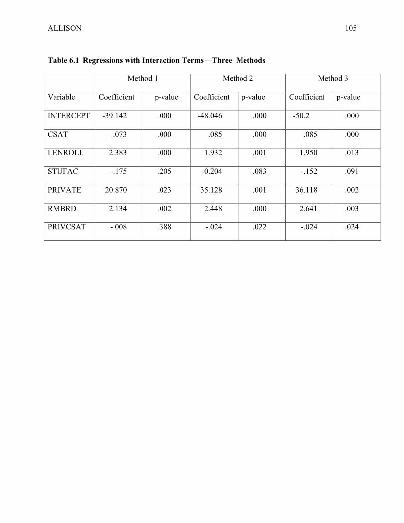
ALLISON 105

Table 6.1 Regressions with Interaction Terms—Three Methods

Method 1 Method 2 Method 3

Variable Coefficient p-value Coefficient p-value Coefficient p-value

INTERCEPT -39.142 .000 -48.046 .000 -50.2 .000

CSAT .073 .000 .085 .000 .085 .000

LENROLL 2.383 .000 1.932 .001 1.950 .013

STUFAC -.175 .205 -0.204 .083 -.152 .091

PRIVATE 20.870 .023 35.128 .001 36.118 .002

RMBRD 2.134 .002 2.448 .000 2.641 .003

PRIVCSAT -.008 .388 -.024 .022 -.024 .024

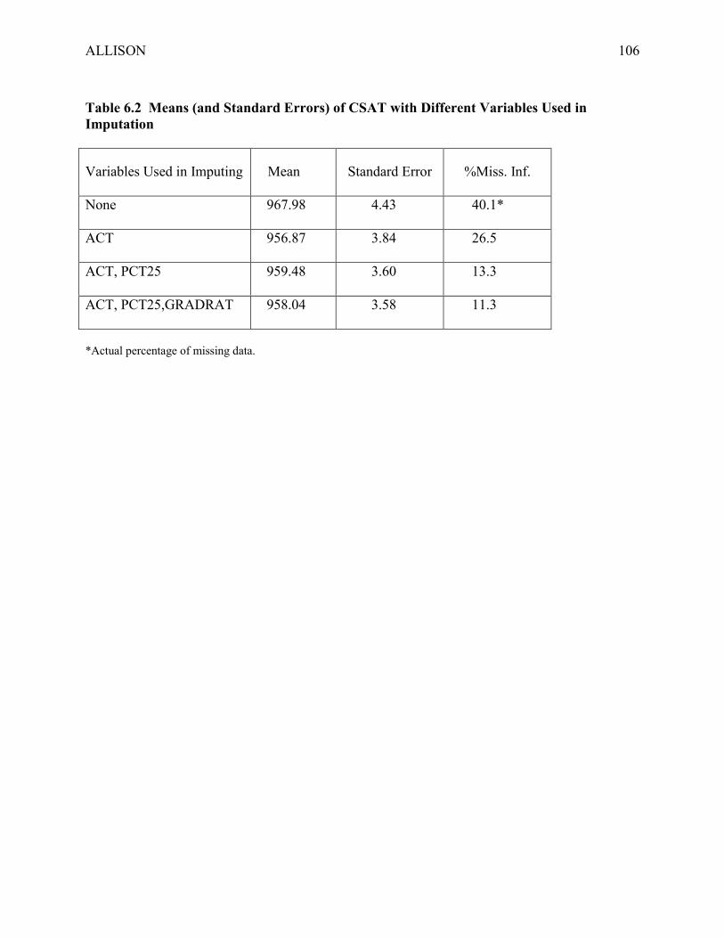
ALLISON 106

Table 6.2 Means (and Standard Errors) of CSAT with Different Variables Used inImputation

Variables Used in Imputing Mean Standard Error %Miss. Inf.

None 967.98 4.43 40.1*

ACT 956.87 3.84 26.5

ACT, PCT25 959.48 3.60 13.3

ACT, PCT25,GRADRAT 958.04 3.58 11.3

*Actual percentage of missing data.

ALLISON 107

Table 6.3 Coefficient Estimates (and Standard Errors) for Cumulative Logit ModelsPredicting SPANKING.

Listwise

Deletion

Normal Data

Augmentation

Sequential

Regression

Seq. Regression

(no missing on

SPANKING)

FEMALE -.355 (.141)* -.481 (.089)*** -.449 (.098)*** -.489 (.094)***

BLACK .565 (.218)** .756 (.117)*** .693 (.119)*** .685 (.135)***

INCOME -.0036 (.0033) -.0052 (.0020)* -.0042 (.0027) -.0047 (.0022)*

EDUC -.055 (.027)* -.061 (.016)*** -.073 (.019)** -.068 (.016)***

NODOUBT .454 (.147)** .465 (.120)** .455 (.156)* .438 (.121)**

NOCHILD -.205 (.199) -.109 (.112) -.141 (.164) -.091 (.123)

AGE .010 (.005)* .0043 (.0032) .0031 (.0032) .0040 (.0031)

EAST -.712 (.219)** -.444 (.125)*** -.519 (.156)** -.488 (.136)***

MIDWEST -.122 (.203) -.161 (.136) -.228 (.149) -.159 (.128)

SOUTH .404 (.191)** .323 (.156)* .262 (.129)* .357 (.121)**

NEVMAR -.046 (.238) -.075 (.148) -.036 (.173) -.071 (.151)

DIVSEP -.191 (.194) -.203 (.150) -.141 (.128) -.184 (.126)

WIDOW .148 (.298) -.244 (.150) -.116 (.177) -.215 (.174)

*p<.05, **p<.01, ***p<.001

ALLISON 108

Table 6.4 Coefficient Estimates (and Standard Errors) for Fixed-Effects Models PredictingCESD.

Listwise

Deletion by

Person

Listwise

Deletion by

Person-Time

Data

Augmentation by

Person-Time

Data

Augmentation by

Person

SRH 2.341 (.586)** 1.641 (.556)** 2.522 (.617)** 1.538 (.501)**

WALK -1.552 (.771)* -1.381 (.761) -1.842 (.960) -.550 (.825)

ADL -.676 (.528) -.335 (.539) -.385 (.562) -.410 (.435)

PAIN .031 (.179) .215 (.168) .305 (.180) .170 (.164)

WAVE 1 8.004 (.650)** 8.787 (.613)** 6.900 (.729)** 9.112 (.615)**

WAVE 2 7.045 (.579)** 7.930 (.520)** 5.808 (.642)** 8.131 (.549)**

N (person-times) 303 453 660 660

*p<.05, **p<.01

ALLISON 109

7. NONIGNORABLE MISSING DATA

Previous chapters have focused on methods for situations in which the missing data

mechanism is ignorable. Ignorability implies that we don’t have to model the process by which

data happen to be missing. The key requirement for ignorability is that the data are missing at

random—the probability of missing data on a particular variable does not depend on the values

of that variable (net of other variables in the analysis).

The basic strategy for dealing with ignorable missing data is easily summarized: adjust

for all observable differences between missing and non-missing cases, and assume that all

remaining differences are unsystematic. This is, of course, a familiar strategy. Standard

regression models are designed to do just that—adjust for observed differences and assume that

unobserved differences are unsystematic.

Unfortunately, there are often strong reasons for suspecting that data are not missing at

random. Common sense tells us, for example, that people who have been arrested are less likely

to report their arrest status than people who have not been arrested. People with high incomes

may be less likely to report their incomes. In clinical drug trials, people who are getting worse

are more likely to drop out than people who are getting better.

What should be done in these situations? There are models and methods for handling

nonignorable missing data, and it is natural to want to apply them. But it is no accident that there

is little software available for estimating nonignorable models (with one important exception—

Heckman’s selectivity bias model). The basic problem is this: given a model for the data, there’s

only one ignorable missing data mechanism but there are infinitely many different nonignorable

missing data mechanisms. So it’s hard to write computer programs that will handle even a

fraction of the possibilities. Furthermore, the answers may vary widely depending the model one

ALLISON 110

chooses. So it’s critically important to choose the right model, and that requires very accurate

and detailed knowledge of the phenomenon under investigation. Worse still, there’s no way to

empirically discriminate one nonignorable model from another (or from the ignorable model).

I won’t go so far as to say “don’t go there” but I will say this. If you choose to go there,

do so with extreme caution. And if you don’t have much statistical expertise, make sure you find

a collaborator who does. Keeping those caveats in mind, this chapter is designed to give you a

brief introduction and overview to some approaches for dealing with nonignorable missing data.

The first thing you need to know is that the two methods I’ve been pushing for ignorable

missing data—maximum likelihood and multiple imputation—can be readily adapted to deal

with nonignorable missing data. If the chosen model is correct (a big if), these two methods

have the same optimal properties that they have in the ignorable setting. A second point to

remember is that any method for nonignorable missing data should be accompanied by a

sensitivity analysis. Since results can vary widely depending on the assumed model, it’s

important to try out a range of plausible models and see if they give similar answers.

Two Classes of Models

Regardless of whether you choose maximum likelihood or multiple imputation, there are

two quite different approaches to modeling nonignorable missing data: selection models and

pattern-mixture models. This is most easily explained for a single variable with missing data.

Let Y be the variable of interest, and let R be a dummy variable with a value of 1 if Y is observed

and 0 if Y is missing. Let f(Y, R) be the joint probability density function (p.d.f.) for the two

variables. Choosing a model means choosing some explicit specification for f(Y, R).

The joint p.d.f. can be factored in two different ways (Little and Rubin 1987). In

selection models we use

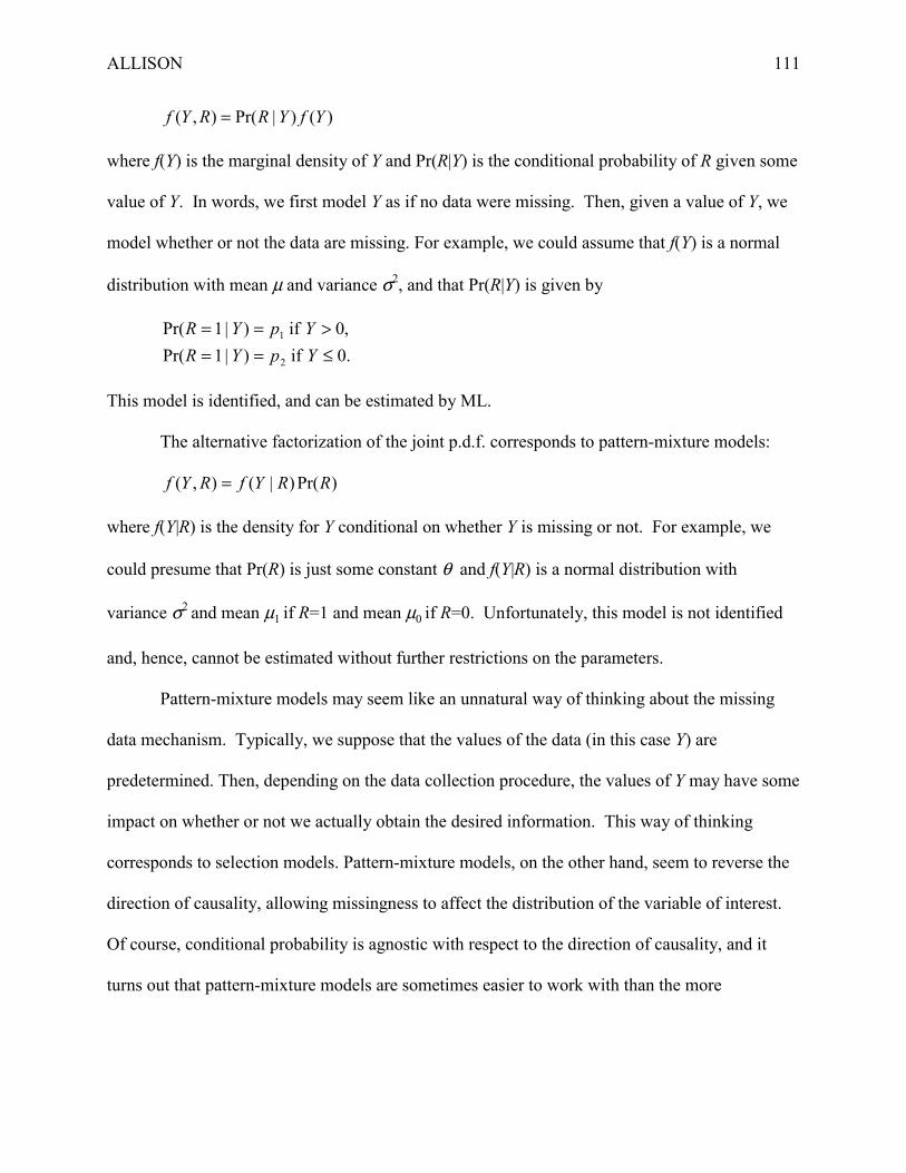
ALLISON 111

)()|Pr(),( YfYRRYf =

where f(Y) is the marginal density of Y and Pr(R|Y) is the conditional probability of R given some

value of Y. In words, we first model Y as if no data were missing. Then, given a value of Y, we

model whether or not the data are missing. For example, we could assume that f(Y) is a normal

distribution with mean µ and variance σ2, and that Pr(R|Y) is given by

.0 if )|1Pr(,0 if )|1Pr(

2

1

≤==>==

YpYRYpYR

This model is identified, and can be estimated by ML.

The alternative factorization of the joint p.d.f. corresponds to pattern-mixture models:

)Pr()|(),( RRYfRYf =

where f(Y|R) is the density for Y conditional on whether Y is missing or not. For example, we

could presume that Pr(R) is just some constant θ and f(Y|R) is a normal distribution with

variance σ2 and mean µ1 if R=1 and mean µ0 if R=0. Unfortunately, this model is not identified

and, hence, cannot be estimated without further restrictions on the parameters.

Pattern-mixture models may seem like an unnatural way of thinking about the missing

data mechanism. Typically, we suppose that the values of the data (in this case Y) are

predetermined. Then, depending on the data collection procedure, the values of Y may have some

impact on whether or not we actually obtain the desired information. This way of thinking

corresponds to selection models. Pattern-mixture models, on the other hand, seem to reverse the

direction of causality, allowing missingness to affect the distribution of the variable of interest.

Of course, conditional probability is agnostic with respect to the direction of causality, and it

turns out that pattern-mixture models are sometimes easier to work with than the more

ALLISON 112

theoretically appealing selection models, especially for multiple imputation. I now consider

some examples of both selection models and pattern-mixture models.

Heckman’s Model for Sample Selection Bias

Heckman’s (1976) model for sample selection bias is the classic example of a selection

model for missing data. The model is designed for situations in which the dependent variable in a

linear regression model is missing for some cases but not for others. A common motivating

example is a regression predicting women’s wages, where wage data are necessarily missing for

women who are not in the labor force. It is natural to suppose that women are less likely to enter

the labor force if their wages would be low. Hence, the data are not missing at random.

Heckman formulated his model in terms of latent variables, but I will work with a more

direct specification. For a sample of n cases (i=1,…, n), let Yi be a normally distributed variable

with a variance σ2 and a mean given by

E(Yi) = βXi (7.1)

where Xi is a column vector of independent variables (including a value of 1 for the intercept)

and β is a row vector of coefficients. The goal is to estimate β. If all Yi were observed, we could

get ML estimates of β by ordinary least squares regression. But some Yi are missing. The

probability of missing data on Yi is assumed to follow a probit model

)(),|0Pr( 210 iiiii XYXYR ααα ++Φ== (7.2)

where Φ(.) is the cumulative distribution function for a standard normal variable. Unless α1=0,

the data are not missing at random because the probability of missingness depends on Y.

This model is identified (even when there are no Xi or when Xi does not enter the probit

equation) and can be estimated by maximum likelihood. The likelihood for an observation with Y

observed is

ALLISON 113

[ ] 1210 )(1)|(),|1Pr( −

��

��

� −++Φ−== σσ

βφααα iiiiiiiii

xyxyxyfxyR . (7.3)

where φ(.) is the density function for a standard normal variable. For an observation with Y

missing, the likelihood is

�∞+

∞−��

�

�

��

�

�

+++Φ==

221

210

1)()|(),|0Pr(

σααβαα i

iiixdyxyfxyR . (7.4)

Eq. (7.4) follows from the general principle that the likelihood for an observation with missing

data can be found by integrating the likelihood over all possible values of the missing data. The

likelihood for the entire sample can be readily maximized using standard numerical methods.

Unfortunately, estimates produced by this method are extremely sensitive to the

assumption that Y has a normal distribution. If Y actually has a skewed distribution, ML

estimates obtained under Heckman’s model may be severely biased, perhaps even more than

estimates obtained under an ignorable missing data model (Little and Rubin 1987).

Heckman also proposed a two-step estimator that is less sensitive to departures from

normality, substantially easier to compute and, therefore, more popular than ML. But the two-

step method has its own limitations.

In brief, the two steps are:

1. Estimate a probit regression of R—the missing data indicator—on the X variables.

2. For cases that have data present on Y, estimate a least-squares linear regression of Y

on X plus a variable that is a transformation of the predicted values from the probit

regression.16

Unlike the ML method, the two-step procedure is not feasible if there are no X variables.

Furthermore, the parameters are only weakly identified if the X variables are the same in the

probit and linear regressions. To get reasonably stable estimates, it is essential that there be X

ALLISON 114

variables in the probit regression that are excluded from the linear regression. Of course, it is

rare that such exclusion restrictions can be persuasively justified. Even when all these conditions

are met, the two-step estimator may perform poorly in many realistic situations (Stolzenberg and

Relles 1990, 1997).

Given the apparent sensitivity of these sample selection methods to violations of

assumptions, how should one proceed to do a sensitivity analysis? For the ML estimator, the key

assumption is the normality of the dependent variable Y. So a natural strategy would be to fit

models that assume different distributions. Skewed distributions like the Weibull or gamma

would probably be most useful since it’s the symmetry of the normal distribution that is most

crucial for ML. ML estimation should be possible for alternative distributions, although the

integral in (7.4) may not have a convenient form and may require numerical integration. For the

two-step estimator, the key assumption is the exclusion of certain X variables from the linear

regression predicting Y. A sensitivity analysis might explore the consequences of choosing

different sets of X variables for the two equations.

ML Estimation with Pattern-Mixture Models

Pattern-mixture models are notoriously underidentified. Suppose we have two variables

X and Y, with four observed patterns of missingness:

1. Both X and Y observed.

2. X observed, Y missing.

3. Y observed, X missing.

4. Both X and Y missing.

Let R=1, 2, 3, or 4, depending on which of these patterns is observed. A pattern-mixture model

for these data has the general form:

ALLISON 115

)Pr()|,(),,( RRXYfRYXf = .

To make the model more specific, we might suppose that Pr(R) is given by the set of values p1,

p2, p3, and p4. Then we might assume that f(Y, X|R) is a bivariate normal distribution with the

usual parameters: XYYXYX σσσµµ ,,,, . However, we allow each of these parameters be different

for each value of R.. The problem is that when X is observed but Y is not, there’s no information

to estimate the mean and standard deviation of Y or the covariance of X and Y. Similarly, when Y

is observed but X is not, there’s no information to estimate the mean and standard deviation of X,

or the covariance of X and Y. And if both variables are missing, we have no information at all.

In order to make any headway, we must impose some restrictions on the four sets of

parameters. Let θ(i) be the set of parameters for pattern i. A simple but very restrictive condition

is to assume that )4()3()2()1( θθθθ === which is equivalent to MCAR. In that case, ML

estimation of the pattern-mixture model is identical to that discussed in Chapter 3 for the normal

model with ignorable missing data. Little (1993, 1994) has proposed other classes of restrictions

that do not correspond to ignorable missing data, but yield identified models. Here’s one

example. Let )(|iXYθ represent the conditional distribution of Y given X for pattern i. What Little

calls complete-case missing-variable restrictions are given by

)1()4(

)1(|

)3(|

)1(|

)2(|

θθ

θθ

θθ

=

=

=

YXYX

XYXY

For the two patterns with one variable missing, the conditional distribution of the missing

variable given the observed variable is equated to the corresponding distribution for the

complete-case pattern. For the pattern with both variables missing, all parameters are assumed

equal to those in the complete-case pattern. This model is identified, and the ML estimates can

ALLISON 116

be found by noniterative means. Once all these estimates are obtained, they can be easily

combined to get estimates of the marginal distribution of X and Y.

Multiple Imputation with Pattern-Mixture Models

ML estimation of pattern mixture models is still rather esoteric at this point in time.

Much more practical and useful is the combination of pattern-mixture models with multiple

imputation (Rubin 1987). The simplest strategy is to first generate imputations under an

ignorable model, and then modify the imputed values using, say, a linear transformation. A

sensitivity analysis is then easily obtained by repeating the process with different constants in the

linear transformation.

Here’s a simple example. Suppose that we again have two variables X and Y but only

two missing data patterns: (1) complete case and (2) missing Y. We assume that within each

pattern, X and Y have a bivariate normal distribution. We also believe that cases with missing Y

tend to be those with higher values of Y. So we assume that all parameters for the two patterns

are the same, except that )1()2(YY cµµ = where c is some constant greater than 1. Multiple

imputation then amounts to generating imputed values for Y under an ignorable missing data

mechanism, and then multiplying all the imputed values by c. Of course, to make this work we

have choose a value for c, and that may be rather arbitrary. A sensitivity analysis consists of re-

imputing the data and re-estimating the model for several different values of c.17

Now let’s turn this into a real example. For the college data, there were 98 colleges with

missing data on the dependent variable, graduation rate. It’s plausible to suppose that those

colleges which didn’t report graduation rates had lower graduation rates than those that did

report their rates. This speculation is supported by the fact that, for the multiply imputed data

described in Chapter 5, the mean of the imputed graduation rates is about 10 percentage points

ALLISON 117

lower than the mean graduation rate for the colleges without missing data. But this difference is

entirely due to differences on the predictor variables, and does not constitute evidence that the

data are not missing at random.

Suppose, however, that the differences in graduation rates between missing and non-

missing cases is even greater. Specifically, let’s modify the imputed graduation rates so that they

are a specified percentage of what would otherwise be imputed under the ignorability

assumption. Table 7.1 displays results for imputations that are 100%, 90%, 80%, 70%, and 60%

of the original values. For each regression, entirely new imputations were generated. Thus,

some of the variation across columns is due to the randomness of the imputation process. In

general, the coefficients are quite stable, suggesting that departures from ignorability would not

have much impact on the conclusions. The STUFAC coefficient varies the most, but it’s far

from statistically significant in all cases.


ALLISON 118

Table 7.1 Regression of Graduation Rates on Several Variables, Under Different Pattern-Mixture Models.

100% 90% 80% 70% 60%

CSAT 0.067 0.069 0.071 0.072 0.071

LENROLL 2.039 2.062 2.077 2.398 2.641

PRIVATE 12.716 12.542 11.908 12.675 12.522

STUFAC -0.217 -0.142 -0.116 -0.126 -0.213

RMBRD 2.383 2.264 2.738 2.513 2.464

ALLISON 119

8. SUMMARY AND CONCLUSION

Among conventional methods for handling missing data, listwise deletion is the least

problematic. Although listwise deletion may discard a substantial fraction of the data, there is no

reason to expect bias unless the data are not missing completely at random. And the standard

errors should also be decent estimates of the true standard errors. Furthermore, if you’re

estimating a linear regression model, listwise deletion is quite robust to situations where there is

missing data on an independent variable and the probability of missingness depends on the value

of that variable. If you’re estimating a logistic regression model, listwise deletion can tolerate

either non-random missingness on the dependent variable or non-random missingness on the

independent variables (but not both).

By contrast, all other conventional methods for handling missing data introduce bias into

the standard error estimates. And many conventional methods (like dummy variable adjustment)

produce biased parameter estimates, even when the data are missing completely at random. So

listwise deletion is generally a safer approach.

If the amount of data that must be discarded under listwise deletion is intolerable, then

two alternatives to consider are maximum likelihood and multiple imputation. In their standard

incarnations, these two methods assume that the data are missing at random, an appreciably

weaker assumption than missing completely at random. Under fairly general conditions, these

methods produce estimates that are approximately unbiased and efficient. They also produce

good estimates of standard errors and test statistics. The downside is that they are more difficult

to implement than most conventional methods. And multiple imputation gives you slightly

different results every time you do it.

ALLISON 120

If the goal is to estimate a linear model that falls within the class of models estimated by

LISREL and similar packages, then maximum likelihood is probably the preferred method.

Currently there are at least four statistical packages that can accomplish this, the best-known of

which is Amos.

If you want to estimate any kind of non-linear model, then multiple imputation is the way

to go. There are many different ways to do multiple imputation. The most widely used method

assumes that the variables in the intended model have a multivariate normal distribution.

Imputation is accomplished by a Bayesian technique that involves iterated regression imputation

with random draws for both the data values and the parameters. Several software packages are

currently available to accomplish this.

Other multiple imputation methods that make less restrictive distributional assumptions

are currently in development. But these have not yet reached a level of theoretical or

computational refinement that would justify widespread use.

It’s also possible to do maximum likelihood or multiple imputation under assumptions

that the data are not missing at random. But getting good results is tricky. These methods are

very sensitive to the assumptions made about the missingness mechanism or about the

distributions of the variables with missing data. And there is no way to test these assumptions.

Hence, the most important requirement is good a priori knowledge of the mechanism generating

the missing data. Any effort to estimate non-ignorable models should be accompanied by a

sensitivity analysis.

ALLISON 121

NOTES

1 The proof is straightforward. We want to estimate f(Y|X), the conditional distribution of Y given X, a vector of

predictor variables. Let A=1if all variables are observed, otherwise 0. Listwise deletion is equivalent to estimating

f(Y|X, A=1). Our aim is to show that this function is the same as f(Y|X). From the definition of conditional

probability, we have

)()|1Pr()()|(),|1Pr(

)1,()1,,()1,|(

XfXAXfXYfXYA

AXfAXYfAXYf

===

====

Assume that Pr(A=1|Y, X) = Pr(A=1|X), i.e., that the probability of data present on all variables does not depend on

Y, but may depend on any variables in X. It immediately follows that

f(Y|X, A=1) = f(Y|X)

Note that this result applies to any regression procedure, not just linear regression.

2 Even if the probability of missing data depends on both X and Y, there are some situations when listwise deletion is

unproblematic. Let p(Y, X) be the probability of missing data on one or more of the variables in the regression

model, as a function of the dichotomous dependent variable Y and a vector of independent variables X. If that

probability can be factored as p(Y, X) = f(Y)g(Y), then logistic regression slopes using listwise deletion are consistent

estimates of the true coefficients (Glynn 1985)

3 Glasser (1964) derived formulas that are reasonably easy to implement, but valid only when the independent

variables and missing data pattern are “fixed” from sample to sample, an unlikely condition for realistic

applications. The formulas of Van Praag et al. (1985) are more generally applicable, but require information beyond

that given in the covariance matrix: higher-order moments and the numbers of available cases for all sets of four

variables.

ALLISON 122

4 While the dummy variable adjustment method is clearly unacceptable when data are truly missing, it may still be

appropriate in cases where the unobserved value simply does not exist. For example, married respondents may be

asked to rate the quality of their marriage, but that question has no meaning for unmarried respondents. Suppose we

assume that there is one linear equation for married couples and another equation for unmarried couples. The

married equation is identical to the unmarried equation except that it has (a) a term corresponding to the effect of

marital quality on the dependent variable and (b) a different intercept. It’s easy to show that the dummy variable

adjustment method produces optimal estimates in this situation.

5 Schafer and Schenker (2000) have proposed a method for getting consistent estimates of the standard errors when

using conditional mean imputation. They claim that, under appropriate conditions, their method can yield more

precise estimates with less computational effort than multiple imputation.

6 Maximum likelihood under the multivariate normal assumption produces consistent estimates of the means and the

covariance matrix for any multivariate distribution with finite fourth moments (Little and Smith 1987).

7 For the two-step method, it’s also possible to get standard error estimates using “sandwich” formulas described by

Browne and Arminger (1995).

8 The standard errors were estimated under the assumption of bivariate normality, which is appropriate for this

example because the data were drawn from a bivariate normal distribution. The formula is

nrres

22 )1().(. −=

While the sample correlation coefficient is not normally distributed, the large sample size in this case should ensure

a close approximation to normality. Thus, these standard errors could be appropriately used to construct confidence

intervals.

9 For data augmentation, the standard noninformative prior (Schafer 1997), known as the Jeffreys prior, is written as

2/)1( +−Σ p where Σ is the covariance matrix and p is the number of variables.

ALLISON 123

10 One way to get such an overdispersed distribution is to use a bootstrap method. For example, one could take five

different random samples, with replacement from the original data set, and compute the EM estimate in each of

these samples. The EM estimates could then be used as starting values in each of five parallel chains.

11 An easy way to do this is to divide the (0,1) interval into five sub-intervals with lengths proportional to the

probabilties for each category of marital status. Draw a random number from a uniform distribution on the unit

interval. Assign the marital status category corresponding to the subinterval in which the random number falls.

12 Actually, the degrees of freedom is equal to the rank of L which is usually, but not always r.

13 The nine regions were classified as follows:

East (New England, Middle Atlantic) 566 cases

Central (East North Central, West North Central) 715 cases

South (South Atlantic, East South Central, West South Central) 1095 cases

West (Mountain, Pacific) 616 cases.

14 The regression analysis was performed with the GLM procedure in SAS using the ABSORB statement to handle

the fixed effects.

15 Ten data sets were produced, with 30 iterations per data set. After imputation, the imputed values were recoded

wherever necessary to preserve the permissible values of the original variables.

16Specifically, the additional variable is λ(axi ) where a is the row vector of estimated coefficients from the probit

model. The function λ(z), the inverse Mills function, is defined asφ(z)/φ(z) whereφ(z) is the density function and

φ(z) is the cumulative distribution function, both for a standard normal variable.

17 In the models considered by Rubin (1987), one specifies the conditional prior distribution of the parameters for

the missing data pattern given the parameters in the complete data pattern. In the example given here, I have merely

assumed that the conditional mean for the missing cases is some multiple of the mean for the complete cases. One

ALLISON 124

may also wish to allow the conditional variance for the missing cases to be larger than that for the complete cases to

allow for greater uncertainty.

ALLISON 125

REFERENCES

Agresti, Alan and Barbara Finlay. 1997. Statistical Methods for the Social Sciences. Upper

Saddle River, NJ: Prentice-Hall.

Allison, Paul D. 1987. “Estimation of Linear Models with Incomplete Data.” Pp. 71-103 in

Clifford Clogg (ed.), Sociological Methodology 1987. Washington, DC: American

Sociological Association.

Allison, Paul D. 2000. “Multiple Imputation for Missing Data.” Sociological Methods &

Research 28: 301-309.

Barnard, John and Donald R. Rubin. 1999. “Small-Sample Degrees of Freedom with Multiple

Imputation.” Biometrika 86: 948-955.

Beale, E. M. L. and Roderick J. A. Little. 1975. “Missing Values in Multivariate Analysis.”

Journal of the Royal Statistical Society, Series B 37: 129-145.

Brand, J.P.L. 1999. Development, Implementation and Evaluation of Multiple Imputation

Strategies for the Statistical Analysis of Incomplete Data Sets. Ph.D. Thesis, Erasmus

University Rotterdam. ISBN 90-74479-08-1.

Browne, M. W. and Gerhard Arminger (1995) “Specification and Estimation of Mean and

Covariance Structure Models.” Pp. 185-249 in G. Arminger, C.C. Clogg and M. E. Sobel

(eds.), Handbook of Statistical Modeling for the Social and Behavioral Sciences.” New

York: Plenum Press.

Cohen, Jacob and Patricia Cohen. 1985. Applied Multiple Regression and Correlation Analysis

for the Behavioral Sciences (2nd ed.). Lawrence Erlbaum Associates.

ALLISON 126

Davis, James A. and Tom W. Smith. 1997. General Social Surveys, 1972-1996: Chicago, IL:

National Opinion Research Center [producer]. Ann Arbor, MI: Inter-university Consortium

for Political and Social Research [distributor].

Dempster, A. P., Nan M. Laird and Donald B. Rubin. 1977. “Maximum Likelihood Estimation

from Incomplete Data Via the EM Algorithm.” Journal of the Royal Statistical Society,

Series B 39: 1-38.

Fuchs, C. 1982. “Maximum Likelihood Estimation and Model Selection in Contingency Tables

with Missing Data.” Journal of the American Statistical Association 77: 270-278.

Glasser, M. 1964. “Linear Regression Analysis with Missing Observations Among the

Independent Variables.” Journal of the American Statistical Association 59: 834-844.

Glynn, Robert. 1985. Regression Estimates When Nonresponse Depends on the Outcome

Variable. Unpublished D.Sc. dissertation. Harvard University School of Public Health.

Gourieroux, Christian and Alain Monfort. 1981. “On the Problem of Missing Data in Linear

Models.” Review of Economic Studies 48: 579-586.

Greene, William H. 2000. Econometric Analysis. 4th Edition. Upper Saddle River, NJ: Prentice-

Hall.

Haitovsky, Yoel. 1968. “Missing Data in Regression Analysis.” Journal of the Royal Statsitical

Society, Series B 30: 67-82.

Heckman, James J. 1976. “The Common Structure of Statistical Models of Truncated, Sample

Selection and Limited Dependent variables, and a Simple Estimator of Such Models.”

Annals of Economic and Social Measurement 5: 475-492.

Iversen, Gudmund. 1985. Bayesian Statistical Inference. Thousand Oaks, CA: Sage

Publications.

ALLISON 127

Jones, Michael P. 1996. “Indicator and Stratification Methods for Missing Explanatory Variables

in Multiple Linear Regression.” Journal of the American Statistical Association 91: 222-

230.

Kim, Jae-On and James Curry. 1977. “The Treatment of Missing Data in Multivariate Analysis.”

Sociological Methods & Research 6: 215-240.

King, Gary, James Honaker, Anne Joseph and Kenneth Scheve. 2000. “Analyzing Incomplete

Political Science Data: An Alternative Algorithm for Multiple Imputation.” Unpublished

paper available at http://gking.harvard.edu/stats.shtml.

King, Gary, James Honaker, Anne Joseph, Kenneth Scheve and Naunihal Singh. 1999.

“AMELIA: A Program for Missing Data.” Unpublished program manual available at

http://gking.harvard.edu/stats.shtml.

Landerman, Lawrence R., Kenneth C. Land and Carl F. Pieper. 1997. “An Empirical Evaluation

of the Predictive Mean Matching Method for Imputing Missing Values.” Sociological

Methods & Research 26: 3-33.

Li, K. H., X. L. Meng, T. E. Raghunathan and Donald B. Rubin. 1991. “Significance Levels

from Repeated p-Values and Multiply Imputed Data.” Statistica Sinica 1: 65-92.

Little, Roderick J. A. 1988. “Missing Data in Large Surveys” (with discussion). Journal of

Business and Economic Statistics 6: 287-201.

Little, Roderick J. A. 1992. “Regression with Missing X’s: A Review.” Journal of the

American Statistical Association 87: 1227-1237.

Little, Roderick J. A. 1993. “Pattern-Mixture Models for Multivariate Incomplete Data.” Journal

of the American Statistical Association 88: 125-134.

ALLISON 128

Little, Roderick J. A. 1994. “A Class of Pattern-Mixture Models for Normal Incomplete Data.”

Biometrika 81: 471-483.

Little, Roderick J. A. and Donald B. Rubin. 1987. Statistical Analysis with Missing Data. New

York: Wiley.

Little, Roderick J. A. and Philip J. Smith. 1987. “Editing and Imputation for Quantitative

Survey Data.” Journal of the American Statistical Association 82: 58-68.

Marini, Margaret Mooney, Anthony R. Olsen, and Donald Rubin. 1979. “Maximum Likelihood

Estimation in Panel Studies with Missing Data.” Pp. 314-357 in Karl F. Schuessler (ed.),

Sociological Methodology 1980. San Francisco: Jossey-Bass.

McCullagh, Peter. 1980. “Regression Models for Ordinal Data” (with discussion). Journal of the

Royal Statistical Society, Series B 42: 109-142.

McLachlan, Geoffrey J. and Thriyambakam Krishnan. 1997. The EM Algorithm and Extensions.

New York: Wiley.

Mossey, Jana M., Kathryn Knott and Rebecka Craik. 1990. “Effects of Persistent Depressive

Symptoms on Hip Fracture Recovery.” Journal of Gerontology: Medical Sciences 45:

M163-168.

Muthén, Bengt, K. Kaplan and M. Hollis. 1987. “On Structural Equation Modeling with Data

that are not Missing Completely at Random.” Psychometrika 42: 431-462.

Raghunathan, Trivellore E., James M. Lepkowski, John Van Hoewyk and Peter Solenberger.

1999. “A Multivariate Technique for Multiply Imputing Missing Values Using a Sequence

of Regression Models.” Unpublished manuscript. Contact [email protected].

Robins, James M. and Naisyin Wang. 2000. “Inference for Imputation Estimators.” Biometrika

87: 113-124.

ALLISON 129

Rubin, Donald B. 1976. “Inference and Missing Data.” Biometrika 63: 581-592.

Rubin, Donald B. 1987. Multiple Imputation for Nonresponse in Surveys. New York: Wiley.

Rubin, Donald B. and Nathaniel Schenker. 1991. “Multiple Imputation in Health-Care

Databases: An Overview and Some Applications.” Statistics in Medicine 10: 585-598.

Schafer, Joseph L. 1997. Analysis of Incomplete Multivariate Data. London: Chapman & Hall.

Schafer, Joseph L and Nathaniel Schenker. 2000. “Inference with Imputed Conditional Means.”

Journal of the American Statistical Association 95: 144-154.

Schenker, Nathaniel and Jeremy M.G. Taylor. 1996. “Partially Parametric Techniques for

Multiple Imputation.” Computational Statistics and Data Analysis 22: 425-446.

Stolzenberg, Ross M. and Daniel A. Relles. 1990. “Theory Testing in a World of Constrained

Research Design: The Significance of Heckman’s Censored Sampling Bias Correction for

Nonexperimental Research.” Sociological Methods & Research 18: 395-415.

Stolzenberg, Ross M. and Daniel A. Relles. 1997. “Tools for Intuition About Sample Selection

Bias and Its Correction.” American Sociological Review 62: 494-507.

Vach, Werner. 1994. Logistic Regression with Missing Values in the Covariates. New York:

Springer-Verlag.

Vach, Werner and M. Blettner. 1991. “Biased Estimation of the Odds Ratio in Case-Control

Studies Due to the Use of Ad Hoc Methods of Correcting for Missing Values for

Confounding Variables.” American Journal of Epidemiology 134: 895-907.

Van Buuren, Stef and Karin Oudshoorn. 1999. “Flexible Multiple Imputation by MICE.” Leiden:

TNO Prevention and Health, TNO-PG 99.054. Available at

http://www.multiple-imputation.com/

ALLISON 130

Van Praag, B. M. S, T. K. Dijkstra, and J. Van Velzen. 1985. “Least-squares Theory Based on

General Distributional Assumptions with an Application to the Incomplete Observations

Problem.” Psychometrika 50: 25-36.

Wang, Naisyin and James M. Robins. 1998. “Large Sample Inference in Parametric Multiple

Imputation.” Biometrika 85: 935-948.

Winship, Christopher and Larry Radbill. 1994. “Sampling Weights and Regression Analysis.”

Sociological Methods & Research 23: 230-257.

ALLISON 131

ABOUT THE AUTHOR

PAUL D. ALLISON is Professor of Sociology at the University of Pennsylvania. He

received his Ph.D. in sociology from the University of Wisconsin in 1976, and did

postdoctoral study in statistics at the University of Chicago and the University of

Pennsylvania. He has published four books and more 25 articles on statistical methods in

the social sciences. These have dealt with a wide variety of methods including linear

regression, loglinear analysis, logit analysis, probit analysis, measurement error,

inequality measures, missing data, Markov processes, and event history analysis. Recent

books include Multiple Regression: A Primer and Logistic Regression Using the SAS

System: Theory and Application. He is currently writing a book on fixed-effects methods

for the analysis of longitudinal data. Each summer he teaches five-day workshops on

event history analysis and categorical data analysis which draw nearly 100 researchers

from around the U.S. His substantive interests include scientists’ careers and theories of

altruistic behavior.

1. INTRODUCTION3 2. ASSUMPTIONS6 3. …nielsen/soci709/cdocs/allison.pdf · novel approaches to...

Documents

Transcript of 1. INTRODUCTION3 2. ASSUMPTIONS6 3. …nielsen/soci709/cdocs/allison.pdf · novel approaches to...