2056 IEEE TRANSACTIONS ON INTELLIGENT …orosz/articles/ITS_2017_Jin.pdf · GE AND OROSZ: OPTIMAL...

2056 IEEE TRANSACTIONS ON INTELLIGENT TRANSPORTATION SYSTEMS, VOL. 18, NO. 8, AUGUST 2017

Optimal Control of Connected Vehicle SystemsWith Communication Delay and

Driver Reaction TimeJin I. Ge and Gábor Orosz

Abstract— In this paper, linear quadratic regulation is usedto obtain an optimal design of connected cruise control (CCC).We consider vehicle strings where a CCC vehicle receivesposition and velocity signals through wireless vehicle-to-vehiclecommunication from multiple vehicles ahead. Communicationdelay, driver reaction time, and heterogeneity of vehicles areconsidered. The optimal feedback law is obtained by minimizinga cost function defined by headway and velocity errors and theacceleration of the CCC vehicle on an infinite horizon. We showthat, by decomposing the optimization problem, the feedbackgains can be obtained recursively as signals from vehicles fartherahead become available, and that the gains decay exponentiallywith the number of cars between the source of the signal andthe CCC vehicle. Such properties allow graceful degradation ofCCC performance under imperfect communication. The effectsof the cost function on the head-to-tail string stability are alsoinvestigated and the robustness against variations in humanparameters is tested. The analytical results are verified bynumerical simulations at the nonlinear level. The results allowus to significantly reduce the complexity of CCC design.

Index Terms— Connected vehicles, delay systems, optimalcontrol.

I. INTRODUCTION

S INCE the invention of the automobile over a century ago,automotive engineers have been trying to improve safety

and passenger comfort and provide higher level of mobilityfor customers. However, during the past decades the level oftraffic congestion has become a bottleneck for mobility, whilestop-and-go traffic significantly impacts the fuel economy ofvehicles [1]. Therefore, for sustainable road transportation, it isnot adequate to simply improve the performance of individualcars, but their impact on traffic flow also needs to be evaluated.Although improving the infrastructure may alleviate trafficcongestion, we may design better controllers for individualvehicles, and use these agents to ’steer’ the traffic flow as amulti-agent system towards more desired states. In this paperwe focus on the latter strategy.

Manuscript received February 1, 2016; revised June 10, 2016, July 30, 2016,and September 18, 2016; accepted November 16, 2016. Date of publicationDecember 12, 2016; date of current version July 31, 2017. This work wassupported by the National Science Foundation under Award 1351456. TheAssociate Editor for this paper was H. A. Rakha.

The authors are with the Department of Mechanical Engineering, Univer-sity of Michigan, Ann Arbor, MI 48109 USA (e-mail: [email protected];[email protected]).

Color versions of one or more of the figures in this paper are availableonline at http://ieeexplore.ieee.org.

Digital Object Identifier 10.1109/TITS.2016.2633164

One primary factor under consideration is the longitudinalcontrol of vehicle motion. Since human drivers have relativelylarge reaction time and limited perception abilities, they oftenperform poorly as controllers for the vehicle. Using adap-tive cruise control (ACC), one may improve the longitudinalcontrol due to faster and more accurate sensing abilities andmore sophisticated control strategies [2], [3]. However, therange sensors (radar, lidar) used for ACC are quite expensiveand the penetration rate of ACC systems has not increasedsignificantly over the last couple of years. Moreover, ACCcannot overcome the limitation that only motion informationof the vehicle immediately ahead can be monitored by rangesensors. This restricts the performance of the cruise controllerand limits our ability to improve the traffic flow.

Therefore, researchers proposed to utilize motion infor-mation about the traffic environment around the vehicleusing wireless vehicle-to-infrastructure (V2I) and vehicle-to-vehicle (V2V) communication [4], [5]. In this case, vehiclesmay be controlled while taking into account traffic flowconditions over a longer spatial horizon. Previous strategiesincluded cooperative adaptive cruise control (CACC) where afixed communication structure is assigned to a group of ACCvehicles, so that a platoon could run with relatively small head-way, while velocity fluctuations are attenuated as propagatingbackwards along the vehicle chain [6]–[9]. Various applicationscenarios have been discussed for CACC, with the focus ondesignated-lane highway driving [10]–[12]. Some researchersare trying to loosen the rigid requirement on communicationtopology for CACC, so that it may deal with more realisticmulti-vehicle formations [13]–[15]. However, such cooperativesystems often rely on existing ACC systems, and thus may belimited in real-traffic implementation.

In [16] and [17] connected cruise control (CCC) wasproposed to maintain smooth traffic flow in mixed systemsof conventional, ACC, and communication-assisted vehicles.The CCC controller receives information about the motion ofmultiple vehicles ahead, and actuates the vehicle or assiststhe driver based on these signals. The controller may includeany signals available and thus allow various connectivitytopologies to form among CCC and non-CCC vehicles. Theinfluence of connectivity structures, signal types, packet drops,and communication delays on the longitudinal dynamics ofvehicular chains has been investigated in [17]–[21]. By tuningthe corresponding control gains one may ensure desiredperformance, such as plant stability (the ability to maintain

1524-9050 © 2016 IEEE. Personal use is permitted, but republication/redistribution requires IEEE permission.See http://www.ieee.org/publications_standards/publications/rights/index.html for more information.

GE AND OROSZ: OPTIMAL CONTROL OF CONNECTED VEHICLE SYSTEMS 2057

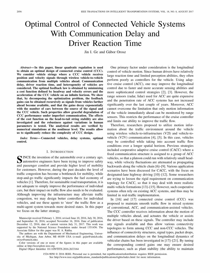
Fig. 1. Functional scheme of the optimal connected cruise control design

chosen speed without external perturbations) and string stabil-ity (the suppression of velocity fluctuations along the vehicularchain). These may have a positive impact on the performanceof the whole transportation system as emphasized by thediagram in Fig. 1.

However, optimality of control gains in terms of mini-mizing velocity fluctuations has not yet been discussed forlarge connected vehicle systems. Optimal CACC designsoften use algorithms with relatively high computational cost,such as rolling horizon optimal control [14], which is onlyfeasible when considering a small group of vehicles withspecific communication structures. Thus, it is necessary tofind optimization algorithms with low computational costfor more general connectivity topologies. While [22] pre-sented some initial ideas about low-cost optimal design, driverreaction time and communication delay were not consid-ered. Here we present an algorithm that is compatible withhuman car-following behaviors while still allowing us to fullyexploit the connectivity without increasing the complexity ofgain-tuning.

In this paper we optimize the gains of a CCC vehiclethat receives position and velocity information from multiplehuman-driven vehicles ahead using linear quadratic regula-tion (LQR). The controller design is based on the minimiza-tion of velocity and headway fluctuations and the controlcost (acceleration/deceleration) for the CCC vehicle. We useoptimization as a tool to observe different levels of relianceon various signals and apply the findings in CCC design.While the optimization is performed over a high-dimensionalnetwork, we show that the problem can be decomposed sincethe information flow is uni-directional in a connected vehiclesystem when vehicles only utilize motion information ofvehicles ahead. Such decomposition allows us to obtain ananalytical solution to the optimization problem recursively, andit allows graceful degradation of CCC performance when V2Vcommunication deteriorates. We also show that the weightsin the cost function can be chosen such that the velocityfluctuations of the CCC vehicle are attenuated compared withvehicles ahead (i.e., string stability can be achieved). While theoptimization is done at the linear level, we demonstrate that thecontroller performs well at the nonlinear level, and is robustagainst parameter variations and heterogeneities appearing inmulti-vehicle systems.

The layout of this paper is as follows. In Section II wepresent models for human driving and build up the modelsfor CCC design. In Section III we introduce the setup of

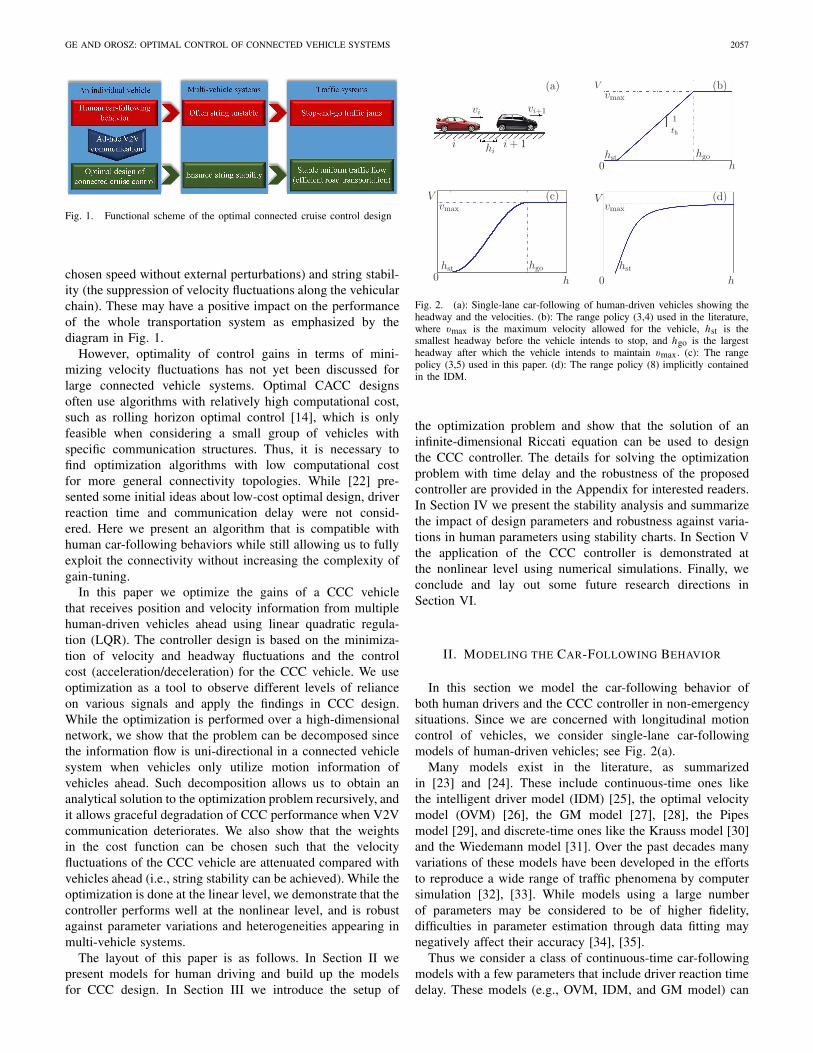
Fig. 2. (a): Single-lane car-following of human-driven vehicles showing theheadway and the velocities. (b): The range policy (3,4) used in the literature,where vmax is the maximum velocity allowed for the vehicle, hst is thesmallest headway before the vehicle intends to stop, and hgo is the largestheadway after which the vehicle intends to maintain vmax. (c): The rangepolicy (3,5) used in this paper. (d): The range policy (8) implicitly containedin the IDM.

the optimization problem and show that the solution of aninfinite-dimensional Riccati equation can be used to designthe CCC controller. The details for solving the optimizationproblem with time delay and the robustness of the proposedcontroller are provided in the Appendix for interested readers.In Section IV we present the stability analysis and summarizethe impact of design parameters and robustness against varia-tions in human parameters using stability charts. In Section Vthe application of the CCC controller is demonstrated atthe nonlinear level using numerical simulations. Finally, weconclude and lay out some future research directions inSection VI.

II. MODELING THE CAR-FOLLOWING BEHAVIOR

In this section we model the car-following behavior ofboth human drivers and the CCC controller in non-emergencysituations. Since we are concerned with longitudinal motioncontrol of vehicles, we consider single-lane car-followingmodels of human-driven vehicles; see Fig. 2(a).

Many models exist in the literature, as summarizedin [23] and [24]. These include continuous-time ones likethe intelligent driver model (IDM) [25], the optimal velocitymodel (OVM) [26], the GM model [27], [28], the Pipesmodel [29], and discrete-time ones like the Krauss model [30]and the Wiedemann model [31]. Over the past decades manyvariations of these models have been developed in the effortsto reproduce a wide range of traffic phenomena by computersimulation [32], [33]. While models using a large numberof parameters may be considered to be of higher fidelity,difficulties in parameter estimation through data fitting maynegatively affect their accuracy [34], [35].

Thus we consider a class of continuous-time car-followingmodels with a few parameters that include driver reaction timedelay. These models (e.g., OVM, IDM, and GM model) can


be written in the form

hi (t) = vi+1(t)− vi (t) ,

vi (t) = F(hi (t − τ ), hi (t − τ ), vi (t − τ )

), (1)

to describe the car-following behavior of vehicle i . Herethe dot stands for differentiation with respect to time t , τis the human reaction time delay, hi denotes the headway,i.e., the bumper-to-bumper distance between vehicle i andits predecessor, and vi denotes the velocity of vehicle i ; seeFig. 2(a). Here we provide some details about the OVMand the IDM that are used very frequently in the literature.However, we remark that the controller design applied in thispaper is applicable to any model of the form (1).

In case of the OVM [18], the vehicle acceleration isdetermined by the difference between the headway-dependentdesired velocity and the actual velocity and by the velocitydifference between the vehicle and its predecessor, that is

F(h, h, v) = α(V (h)− v

) + βh , (2)

where the gains α and β are used by the human drivers tocorrect velocity errors. The desired velocity is determined bythe headway using the continuous range policy

V (h) =

⎧⎪⎨

⎪⎩

0 if h ≤ hst ,

fv(h) if hst < h < hgo ,

vmax if h ≥ hgo ,

(3)

i.e., the desired velocity is zero for small headways (h ≤ hst)and equal to the maximum speed vmax for large headways(h ≥ hgo). Between these, the desired velocity is given byfv(h) which increases with the headway monotonically. Thereare many choices for the specific function of fv(h), but thequalitative dynamics remain similar if the above characteristicsare kept [18], [19]. In [12] the function

fv(h) = vmaxh − hst

hgo − hst(4)

was used, which corresponds to the constant time headwayth = (hgo − hst)/vmax, as shown in Fig. 2(b). However, therange policy (3,4) is non-smooth at h = hst and h = hgo andmay generate a "jerky ride". Thus, here we use

fv(h) = vmax

2

(1 − cos

(π

h − hst

hgo − hst

))(5)

as shown in Fig. 2(c). The range policy (3,5) is smooth buthas a changing time headway given by th = 1/ f ′

v(h).We assume that human-driven vehicles try to maintain the

uniform traffic flow equilibrium

hi (t) ≡ h∗ , vi (t) ≡ v∗ , (6)

given by F(h∗, 0, v∗) = 0, cf. (1). Using (2) we find theequilibrium speed-headway relation of OVM given by its rangepolicy function (3), i.e., v∗ = V (h∗).

On the other hand, the IDM [25] can be written in the form

F(h, h, v)

= a

(1 −

( v

vmax

)4−(hst + Tgapv − hv/

√4ab

h

)2), (7)

where a is the maximum desired acceleration, Tgap is thedesired time gap, and b is the comfortable acceleration. While(7) does not contain a range policy function explicitly, theequilibrium speed-headway relation

h∗ = V −1(v∗) = hst + Tgapv∗

√1 − (v∗/vmax)4

, (8)

shown in Fig. 2(d), describes qualitatively the same drivingbehavior as in Fig. 2(b,c). Notice that for h∗ < hst, we havev∗ < 0 in the IDM, which can be eliminated by requiringvehicle velocities to be non-negative.

Observe that both the OVM (1,2) and the IDM (1,7) can belinearized into the same form [18]. Here we use the particularform (2) when performing the linearization (as the parametersα and β have clear physical meaning), but all results canbe generalized for an arbitrary F(h, h, v). By assuming thesystem in the vicinity of the equilibrium (6) and defining theheadway and velocity perturbations

hi (t) = hi (t)− h∗, vi (t) = vi (t)− v∗ , (9)

we linearize (1,2) to obtain the linear delay differential equa-tion (DDE)

˙hi (t)= vi+1(t)− vi (t) ,˙vi (t)= α

(N∗hi (t−τ )−vi(t−τ )

)+β(vi+1(t−τ )−vi (t−τ )

).

(10)

Here N∗ = V ′(h∗) is the derivative of the range policy (3) atthe equilibrium, and for hst ≤ h∗ ≤ hgo this gives the timeheadway th = 1/ f ′

v(h∗) = 1/N∗.

Controllers with a small time headway produce moreaggressive car-following behaviors, which makes it more dif-ficult to maintain uniform traffic flow [36]. Based on highwaytraffic data [18], we set vmax = 30 [m/s], hst = 5 [m],hgo = 35 [m]. We find at v∗ = 15 [m/s], h∗ = 20 [m] therange policy (3,5) has the largest derivative N∗ = π/2 [1/s]and correspondingly the smallest time headway th ≈ 0.64 [s].We consider this least-string-stable operating point in theremainder of this paper.

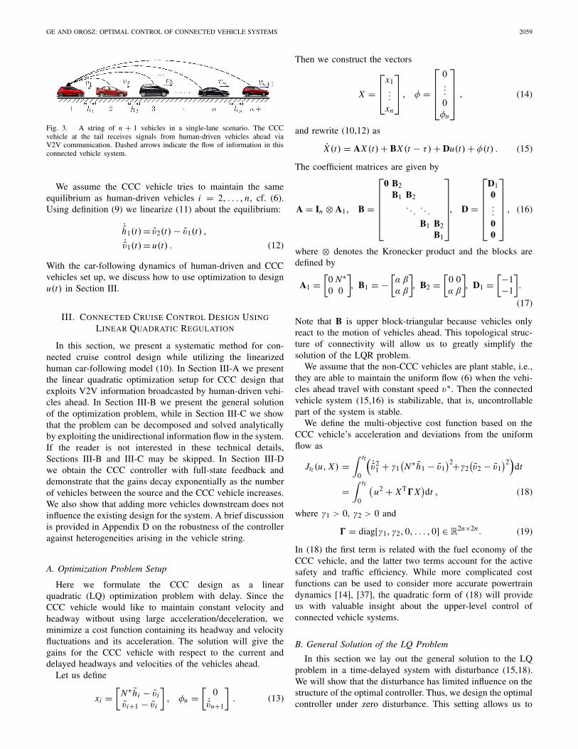
We now consider the single-lane configuration shown inFig. 3 where the CCC vehicle at the tail receives position andvelocity signals of the n non-CCC vehicles ahead through V2Vcommunication (see dashed arrows from preceding vehicles tovehicle 1). Initially, we assume that all preceding vehicles areidentical human-driven vehicles, but the effects of heteroge-neous dynamics among preceding vehicles will be investigatedin Appendix D.

The car-following dynamics of the CCC vehicle is given by

h1(t) = v2(t)− v1(t) ,

v1(t) = u(t) , (11)

where u(t) is the acceleration that will be designed using thevelocity and headway information obtained via V2V commu-nication. Communication delay is not included explicitly in theoptimization, but will be added when analyzing the stabilityof CCC in Section IV.


Fig. 3. A string of n + 1 vehicles in a single-lane scenario. The CCCvehicle at the tail receives signals from human-driven vehicles ahead viaV2V communication. Dashed arrows indicate the flow of information in thisconnected vehicle system.

We assume the CCC vehicle tries to maintain the sameequilibrium as human-driven vehicles i = 2, . . . , n, cf. (6).Using definition (9) we linearize (11) about the equilibrium:

˙h1(t)= v2(t)− v1(t) ,˙v1(t)= u(t) . (12)

With the car-following dynamics of human-driven and CCCvehicles set up, we discuss how to use optimization to designu(t) in Section III.

III. CONNECTED CRUISE CONTROL DESIGN USING

LINEAR QUADRATIC REGULATION

In this section, we present a systematic method for con-nected cruise control design while utilizing the linearizedhuman car-following model (10). In Section III-A we presentthe linear quadratic optimization setup for CCC design thatexploits V2V information broadcasted by human-driven vehi-cles ahead. In Section III-B we present the general solutionof the optimization problem, while in Section III-C we showthat the problem can be decomposed and solved analyticallyby exploiting the unidirectional information flow in the system.If the reader is not interested in these technical details,Sections III-B and III-C may be skipped. In Section III-Dwe obtain the CCC controller with full-state feedback anddemonstrate that the gains decay exponentially as the numberof vehicles between the source and the CCC vehicle increases.We also show that adding more vehicles downstream does notinfluence the existing design for the system. A brief discussionis provided in Appendix D on the robustness of the controlleragainst heterogeneities arising in the vehicle string.

A. Optimization Problem Setup

Here we formulate the CCC design as a linearquadratic (LQ) optimization problem with delay. Since theCCC vehicle would like to maintain constant velocity andheadway without using large acceleration/deceleration, weminimize a cost function containing its headway and velocityfluctuations and its acceleration. The solution will give thegains for the CCC vehicle with respect to the current anddelayed headways and velocities of the vehicles ahead.

Let us define

xi =[

N∗hi − vi

vi+1 − vi

], φn =

[0

˙vn+1

]. (13)

Then we construct the vectors

X =⎡

⎢⎣

x1...

xn

⎤

⎥⎦ , φ =

⎡

⎢⎢⎢⎣

0...0φn

⎤

⎥⎥⎥⎦, (14)

and rewrite (10,12) as

X(t) = AX (t)+ BX (t − τ )+ Du(t)+ φ(t) . (15)

The coefficient matrices are given by

A = In ⊗ A1, B =

⎡

⎢⎢⎢⎢⎢⎣

0 B2B1 B2

. . .. . .

B1 B2B1

⎤

⎥⎥⎥⎥⎥⎦, D =

⎡

⎢⎢⎢⎢⎢⎣

D10...00

⎤

⎥⎥⎥⎥⎥⎦, (16)

where ⊗ denotes the Kronecker product and the blocks aredefined by

A1 =[

0 N∗0 0

], B1 = −

[α βα β

], B2 =

[0 0α β

], D1 =

[−1−1

].

(17)

Note that B is upper block-triangular because vehicles onlyreact to the motion of vehicles ahead. This topological struc-ture of connectivity will allow us to greatly simplify thesolution of the LQR problem.

We assume that the non-CCC vehicles are plant stable, i.e.,they are able to maintain the uniform flow (6) when the vehi-cles ahead travel with constant speed v∗. Then the connectedvehicle system (15,16) is stabilizable, that is, uncontrollablepart of the system is stable.

We define the multi-objective cost function based on theCCC vehicle’s acceleration and deviations from the uniformflow as

Jtf (u, X) =∫ tf

0

( ˙v21 + γ1

(N∗h1 − v1

)2+γ2(v2 − v1

)2)

dt

=∫ tf

0

(u2 + XT�X

)dt , (18)

where γ1 > 0, γ2 > 0 and

� = diag[γ1, γ2, 0, . . . , 0] ∈ R2n×2n . (19)

In (18) the first term is related with the fuel economy of theCCC vehicle, and the latter two terms account for the activesafety and traffic efficiency. While more complicated costfunctions can be used to consider more accurate powertraindynamics [14], [37], the quadratic form of (18) will provideus with valuable insight about the upper-level control ofconnected vehicle systems.

B. General Solution of the LQ Problem

In this section we lay out the general solution to the LQproblem in a time-delayed system with disturbance (15,18).We will show that the disturbance has limited influence on thestructure of the optimal controller. Thus, we design the optimalcontroller under zero disturbance. This setting allows us to


exploit the uni-directional information flow to alleviate thehigh computational cost for optimal connected vehicle design.Readers not interested in the technical details may proceed toSection III-D.

We define the augmented state Y (t) = [XT(t) 1]T to placethe disturbance term φ(t) in (15) into a time-variant coefficientmatrix. This yields

Y (t) = A(t)Y (t)+ BY (t − τ )+ Du(t) , (20)

where

A(t) =[

A φ(t)0 0

], B =

[B 00 0

], D =

[D0

]. (21)

The cost function (18) can be rewritten accordingly

Jtf (u,Y ) =∫ tf

0

(u2 + Y T�Y

)dt , (22)

where � =[� 00 0

].

The optimal control for (20,22) is given by

u(t) = −DT(

P(t)Y (t)+∫ 0

−τQ(t, θ)Y (t + θ)dθ

), (23)

see [38]. The matrices P(t) and Q(t, θ) are obtained by solvingthe Riccati-type partial differential equation (PDE)

−P(t) = ATP(t)+ P(t)A − P(t)DDTP(t)

+ Q(t, 0)+ QT(t, 0)+ � ,

(∂θ − ∂t )Q(t, θ) = (AT − PDDT)

Q(t, θ)+ R(t, 0, θ) ,

(∂ξ + ∂θ − ∂t )R(t, ξ, θ) = −QT(t, ξ)DDTQ(t, θ) , (24)

with boundary conditions

P(tf) = 0 ,

Q(tf, θ) = 0 , Q(t,−τ ) = PTB ,

R(tf , ξ, θ) = 0 , R(t,−τ, θ) = BTQ(t, θ) , (25)

where P(t) is symmetric and RT(t, ξ, θ) = R(t, θ, ξ). Giventhe structure of coefficient matrices (21), the matrices P(t),Q(t, θ) and R(t, ξ, θ) can be constructed as

P =[

P1 P2P3 P4

], Q =

[Q1 Q2Q3 Q4

], R =

[R1 R2R3 R4

], (26)

where P1,Q1,R1 ∈ R2n×2n , P2,Q2,R2 ∈ R

2n×1,P3,Q3,R3 ∈ R

1×2n , and P4,Q4,R4 are scalars. since P(t) issymmetric we have P1(t) = PT

1 (t) and P2(t) = PT3 (t). More-

over, R(t, ξ, θ) = RT(t, θ, ξ) yields R1(t, ξ, θ) = RT1 (t, θ, ξ)

and R2(t, ξ, θ) = RT3 (t, θ, ξ). Thus, the optimal controller

(23) becomes

u(t) = −DT(

P1(t)X (t)+∫ 0

−τQ1(t, θ)X (t + θ)dθ

+ P2(t)+∫ 0

−τQ2(t, θ)dθ

). (27)

By substituting (26) into (24,25) we find that state-feedback-control gain matrices P1,Q1 in the optimal controller (27)are not influenced by the disturbance φ(t); see (65,67,69,71)in Appendix A. On the other hand, when including the

disturbance in the optimization, (27) cannot be implementedin real time since φ(t) is not known a priori; cf. A(t) in(21,24,26). Therefore we first ignore the disturbance φ(t), butlater in Section IV we ensure that this zero-disturbance designcan reject disturbances satisfyingly. Thus, we consider

P2(t) ≡ 0 , Q2(t, θ) ≡ 0 , (28)

which allows us to design the CCC controller analyticallywithout impairing the stability of the multi-vehicle system.

Since P1(t),Q1(t, θ),R1(t, ξ, θ) are given by (65), whichis an initial value problem in backward time, we consider thesteady-state solution

P1(t) ≡ P1, Q1(t, θ) ≡ Q1(θ), R1(t, ξ, θ) ≡ R1(ξ, θ),

(29)

which is equivalent to setting time horizon tf → ∞ in the costfunction (18); see [39].

Substituting (28,29) into (27) leads to the simplified con-troller

u(t) = −DT(

P1 X (t)+∫ 0

−τQ1(θ)X (t + θ)dθ

), (30)

where the matrices P1, Q1(θ) are given by

ATP1 + P1A − P1DDTP1 + Q1(0)+ QT1 (0)+ � = 0 ,

∂θQ1(θ) = (AT − P1DDT)

Q1(θ)+ R1(0, θ) ,

(∂ξ + ∂θ )R1(ξ, θ) = −QT1 (ξ)DDTQ1(θ) , (31)


Q1(−τ ) = P1B , R1(−τ, θ) = BTQ1(θ) , (32)

which can be attained by setting tf → ∞ in (65,66).

C. Decomposition of the Solution

In this section, we exploit the uni-directional informationflow and obtain the analytical solution to the delayed LQproblem (15,18) with zero disturbance (φ(t) ≡ 0) and infinitetime horizon (tf = ∞), i.e., we solve the PDE (31,32)analytically to obtain the controller (30).

While a numerical scheme for (31,32) is given in [39] toobtain P1, Q1(θ) in (30), no closed-form solution exists withgeneral A,B,D matrices. However, here only the first tworows of P1,Q1(θ) are used by the controller (30), since D iszero except its first two elements, cf. (16,17). Thus we onlyneed to obtain an analytical solution for the relevant parts inP1, Q1(θ), which is made possible by taking advantage of theupper-triangular block structure of A and B.

We introduce the notation

P1 =⎡

⎢⎣

P11· · ·P1n.... . .

...Pn1· · ·Pnn

⎤

⎥⎦ , Q1(θ) =

⎡

⎢⎣

Q11(θ)· · · Q1n(θ)...

. . ....

Qn1(θ)· · · Qnn(θ)

⎤

⎥⎦ , (33)

where Pi j ,Qi j (θ) ∈ R2×2 for i, j = 1, . . . , n, and rewrite (30)

as

u(t) = −DT1

n∑

i=1

(P1i xi (t)+

∫ 0

−τQ1i(θ)xi (t + θ)dθ

), (34)


where xi (t) is given in (13). This shows that we only need toderive P1i ,Q1i (θ) for i = 1, . . . , n to construct the controller.Substituting (33) into (31,32), we obtain equations for eachblock Pi j ,Qi j (θ),Ri j (ξ, θ), i, j = 1, . . . , n, which can besolved recursively. Specifically, P11 and Q11(θ) are given by

A1P11 + P11A1 + Q11(0)+ QT11(0)+ diag[γ1, γ2] = 0 ,

∂θQ11(θ) = A1Q11(θ)+ R11(0, θ) ,

(∂ξ + ∂θ )R11(ξ, θ) = −QT11(ξ)DDTQ11(θ) , (35)


Q11(−τ ) = 0 , R11(−τ, θ) = 0 , (36)

where

A1 = AT1 − P11D1DT

1 . (37)

The solution of (35,36) is given by

P11 =[

p11 p12p12 p22

], Q11(θ) ≡ 0, R11(ξ, θ) ≡ 0 , (38)

where

p11 = −γ1 + √γ1

√γ1 + γ2 + 2N∗√γ1

N∗ ,

p12 = √γ1 − p11 ,

p22 = −2√γ1 +

√γ1 + γ2 + 2N∗√γ1 + p11 , (39)

which is the only solution satisfying the condition P11 > 0.Notice that the matrix P11 only depends on the weights γ1, γ2and the CCC vehicle’s range policy N∗ (cf. (3)).

Then, to obtain P1i ,Q1i (θ),Qi1(θ) for i = 2, . . . , n, weneed to solve

A1P1i + P1i A1 + Q1i(0)+ QTi1(0) = 0 ,

∂θQ1i (θ) = A1Q1i (θ)+ R1i (0, θ) ,

∂θQi1(θ) = AT1 Qi1(θ)− PT

1iD1DT1 Q11(θ)+ RT

1i (θ, 0) ,

(∂ξ + ∂θ )R1i (ξ, θ) = −QT11(ξ)D1DT

1 Q1i (θ) , (40)


Q1i(−τ ) = P1i B1 + P1(i−1)B2 ,

Qi1(−τ ) = 0 ,

R1i (θ,−τ ) = QTi1(θ)B1 + QT

(i−1)1(θ)B2 ,

R1i (−τ, θ) = 0 . (41)

Now (40,41) give the solution

Qi1(θ) ≡ 0, R1i(ξ, θ) ≡ 0 , (42)

while the equations for Q1i (θ) simplify to

∂θQ1i (θ) = A1Q1i (θ),

Q1i (−τ ) = P1iB1 + P1(i−1)B2 , (43)

yielding the solution

Q1i (θ) = eA1(θ+τ )(P1i B1 + P1(i−1)B2) , (44)

for i = 2, . . . , n. Thus, the equation for P1i becomes

A1P1i + P1i A1 + eτ A1(P1iB1 + P1(i−1)B2) = 0 , (45)

yielding the solution

vec(P1i ) = Mi−1vec(P11) , (46)

for i = 2, . . . , n. Here vec(·) gives a column vector bystacking the columns of the matrix on the top of each other,and M ∈ R

4×4 is given by

M = −(I ⊗ A1 + AT

1 ⊗ I + BT1 ⊗ eτ A1

)−1(BT2 ⊗ eτ A1

).

(47)

Consequently, P1i and Q1i (θ) are obtained recursively using(38,44,46,47). The recursive rules (44,46) indicate that thefeedback gains for signals coming from the j th vehicle onlydepend on the dynamics of vehicles 2 to j and do not dependon the dynamics of vehicles in front of the j th vehicle. On theother hand, since A1 only depends on P11 (cf. (37,38,39)),the exponential term eA1(θ+τ ) shared by every Q1i(θ) isindependent from the dynamics of preceding vehicles butchanges with the CCC vehicle’s range policy N∗ and theoptimization weights γ1, γ2.

D. Constructing the CCC Controller

In (34) we move D1 (cf. (16)) into the integral and define[α1i β1i

] = [1 1

]P1i ,[

fi (θ) gi (θ)] = [

1 1]

Q1i (θ) . (48)

Based on definitions (13,48), the optimal controller (34) forthe CCC vehicle is given by

u(t) =n∑

i=1

(α1i

(N∗hi (t)−vi (t)

) + β1i(vi+1(t)−vi (t)

))

+n∑

i=1

∫ 0

−τfi (θ)

(N∗hi (t + θ)− vi (t + θ)

)dθ

+n∑

i=1

∫ 0

−τgi (θ)

(vi+1(t + θ)− vi (t + θ)

)dθ , (49)

where the distribution kernels take the form

fi (θ) = (ai0 + ai1(θ + τ )

)eλ1(θ+τ ) + ai2eλ2(θ+τ ) ,

gi (θ) = (bi0 + bi1(θ + τ )

)eλ1(θ+τ ) + bi2eλ2(θ+τ ) , (50)

for i = 1, . . . , n, θ ∈ [−τ, 0], where λ1, λ2 are the eigen-values of A1, and the expressions for λ1, λ2, ai0, ai1, ai2, andbi0, bi1, bi2 are given in Appendix B.

From (38,39,48) we obtain that

α11 = √γ1, β11 = −√

γ1 +√γ1 + γ2 + 2N∗√γ1 , (51)

i.e., the gains on CCC vehicle’s own headway and velocity donot depend on the dynamics of human-driven vehicles. SinceQ11(θ) ≡ 0, (48) yields

f1(θ) ≡ 0, g1(θ) ≡ 0 , (52)

i.e., the CCC vehicle does not have delayed feedback terms onits own headway and velocity. The rest of the gains α1i , β1i

and the distribution kernels fi (θ), gi (θ) for i = 2, . . . , nin (48) can be obtained using (44,46,47).


Fig. 4. The optimized feedback gains α1i , β1i , i = 1, . . . , n of the CCCvehicle in a string of (n + 1) vehicles for n = 5 (red circles) and for n = 10(blue crosses). The human parameters are α = 0.6 [1/s], β = 0.9 [1/s],τ = 0.4 [s]. The design parameters are γ1 = 0.04 [1/s2], γ2 = 0.30 [1/s2].

In Appendix C we show that the eigenvalues of M (cf. (47))are inside the unit circle for realistic values of weights γ1, γ2,human gains α, β, and driver reaction time τ . Thus (46) isa contracting map. Since α1i , β1i are given in (48) as linearcombinations of the components of P1i , they converge to zeroas i increases.

Fig. 4 shows the corresponding exponential decay of α1i

and β1i in a (5 + 1) vehicle chain (red circles) and a (10 + 1)vehicle chain (blue crosses) using the parameter valuesγ1 = 0.04 [1/s2], γ2 = 0.30 [1/s], α = 0.6 [1/s],β = 0.9 [1/s] and τ = 0.4 [s]. In this case, M has two zeroeigenvalues and two non-zero eigenvalues 0.69 ± 0.15i . Theexact match between the red circles and the blue crosses forvehicles 2 to 5 demonstrates that the existing optimized gainsdo not change when adding feedback terms on vehicles fartheraway. This corresponds to the fact that the gains α11, β11 arenot influenced by the connectivity structure (cf. (38,39,48)),and that α1i , β1i are calculated recursively using (46).For the parameters considered above, we have the gainsα11 ≈ 0.20 [1/s], β11 ≈ 0.78 [1/s].

In Fig. 5 we plot the distribution kernels fi (θ), gi(θ) fori = 2, . . . , n using the same parameters as in Fig. 4. Thedashed red curves correspond to n = 5 and the blue solidcurves correspond to n = 10. In both cases, the magnitudeof fi (θ) and gi (θ) decreases with i . Indeed, for vehiclesi = 2, . . . , 5, the distribution kernels fi (θ) and gi (θ) are thesame in both the (5 + 1)-car and the (10 + 1)-car systems.

Considering the similar feedback structure of the CCCcontroller (49) as in the conventional driving model (2), andthe decay of feedback gains and distribution kernels shownin Fig. 4 and Fig. 5, we conclude that the proposed CCCcontroller will degrade gracefully under imperfect commu-nication. More specifically, a CCC vehicle may experiencesevere packet drops from vehicles ahead, depending on theinvolved V2V communication devices, the physical distancebetween vehicles and the road environment [40]. When thecommunication channel with vehicle i +1 significantly deteri-orates, we may set the feedback gains and distribution kernelscorresponding to vehicle i + 1 and vehicles farther ahead aszero, and only use motion signals up to vehicles i . Sincemotion signals from farther downstream vehicles are assignedwith smaller gains, the switch to fewer signals will not inducea significant jump in control commands. Most importantly,since the gains for signals coming from vehicles 1–i do not

Fig. 5. The optimized distribution kernels fi (θ), gi (θ) for i = 2, . . . , nof the CCC vehicle for a (n + 1)-car system with the same parameter as inFig. 4. The red dashed curves correspond to n = 5, and the blue solid curvescorrespond to n = 10. The black arrows show the direction of increasingvehicle index i .

depend on those from vehicles i + 1 and beyond, the reducedCCC controller still remains optimal.

We note that the proposed CCC controller generates 2nfeedback gains and distribution kernels with only 2 designparameters, while being robust against heterogeneity andconnectivity structure changes among preceding vehicles, asdiscussed in detail in Appendix D. While our design relies oncar-following models in the form of (1) for the human-drivenvehicles ahead, one may use other driver models (see [23]) todesign similar controllers.

IV. STABILITY ANALYSIS OF OPTIMIZED CONNECTED

VEHICLE SYSTEMS

In this section, we analyze the linear stability of uniformtraffic flow using the optimized controller for the CCC vehicleat the tail, to make sure that the arising connected vehiclesystem is able to maintain uniform traffic flow. Here we takeinto account the communication delay due to intermittencyand packet loss in wireless communication. We analyze theplant stability and head-to-tail string stability and visualizethe corresponding stability areas using stability charts.

The intermittency in V2V communication with digital con-trollers results in an average communication delay of 0.15 [s];see [16]. However, packet losses may lead to significantincrease of the delay. While the delay changes stochasti-cally [20], here we approximate it with its average and studythe dynamics while viewing the delay as a parameter. Thenthe linear dynamics (10,12) becomes

˙h1(t) = v2(t)− v1(t) ,˙v1(t) = u(t − σ) ,˙hi (t) = vi+1(t)− vi (t) ,˙vi (t) = α

(N∗hi (t−τ )−vi(t−τ )

)

+ β(vi+1(t−τ )−vi(t−τ )

), (53)

for i = 2, . . . , n, where u(t) is given by (49) and σ denotesthe communication delay.

The plant stability of a CCC vehicle is given as follows:suppose that the vehicles whose signals are used by theCCC vehicle are driven at the same constant velocity, thatis, vi (t) ≡ v∗, i = 2, . . . , n + 1, then the velocity of the CCCvehicle approaches this constant velocity, i.e., lim

t→∞ v1(t) = v∗.


The plant stability of non-CCC vehicles is defined similarly:when the preceding vehicle is driven at constant velocity,the non-CCC vehicle should converge to the same veloc-ity. In this paper we only consider plant stable non-CCCvehicles.

String stability characterizes the attenuation of velocityfluctuations as they propagate upstream [36]. For non-CCCvehicles it is required that the vehicle attenuates the velocityfluctuations arising from the preceding vehicle. For a CCCvehicle, one may compare its velocity fluctuations with anypreceding vehicle whose signals is used by the CCC vehicle.The influence of a CCC vehicle on the traffic flow is evaluatedthe best by comparing its velocity fluctuations to that of thefurthest vehicle ahead whose signal is received by the CCCvehicle (called the head vehicle). Thus, we define the head-to-tail string stability, which requires velocity fluctuations tobe suppressed from the head vehicle to the tail. Since nocontrol is placed upon the non-CCC vehicles, it is reasonableto allow amplification of velocity fluctuations among non-CCCvehicles. Still, the CCC vehicles may ensure head-to-tail stringstability as demonstrated below.

While in the previous section the controller was designed forthe zero disturbance case, here we consider the velocity per-turbation vn+1 of the head vehicle as the input and the velocityperturbation v1 of the tail vehicle as the output in (53). Sinceperturbations of velocity can be represented using Fouriercomponents and superposition holds for linear systems, thehead-to-tail string stability can be ensured by attenuating sinu-soidal signals for all excitation frequencies. Thus, we considerthe periodic excitation vn+1(t) = v

ampn+1 sin(ωt) with frequency

ω and amplitude vampn+1. Then the steady state response of (53)

with control (49) is v1,ss(t) = vamp1 sin(ωt + ψ). In order to

ensure head-to-tail string stability, we need the amplitude ratiov

amp1 /v

ampn+1 < 1 for all excitation frequencies ω > 0, which can

be obtained through transfer functions.In particular, taking the Laplace transform of (53) with zero

initial conditions and eliminating the velocities and headwaysof vehicles i = 2, . . . , n, we obtain the head-to-tail transferfunction

H (s) = V1(s)

Vn+1(s)

=

n∑

i=2

(Fi−1(s)− Gi (s)

) · (H0(s)

)n−i+1 + Fn(s)

s2eσ s + G1(s).

(54)

Here V1(s) and Vn+1(s) denote the Laplace transform of v1(t)and vn+1(t), respectively, and

H0(s) = F0(s)

G0(s)= βs + αN∗

s2eτ s + (α + β)s + αN∗ ,

Fi (s) = α1i N∗ + β1i s + (ai1 N∗ + bi1s)h1(s)

+ (ai0 N∗ + bi0s)h0(s)+ (ai2 N∗ + bi2s)h2(s) ,

Gi (s) = Fi (s)+ α1i s + s(ai0h0(s)+ ai1h1(s)+ ai2h2(s)

),

(55)

where ai0, ai1, ai2, bi0, bi1, bi2 are given in Appendix B fori = 1, . . . , n and

h0(s) = eτλ1 − e−τ s

s + λ1,

h1(s) = τe−τ s

s + λ1− eτλ1 − e−τ s

(s + λ1)2,

h2(s) = eτλ2 − e−τ s

s + λ2. (56)

Here H0(s) represents the transfer function between a non-CCC vehicle and its predecessor. Indeed, the amplitude ratiofor frequency ω is given by vamp

1 /vampn+1 = |H (iω)|, that is, the

head-to-tail string stability is ensured when |H (iω)| < 1 forall ω > 0.

A. Plant Stability

The plant stability for the linearized connected vehiclesystem (49,53) requires that all its characteristic roots havenegative real parts, i.e., the solutions of the characteristicequation

Gn−10 (s)

(s2eσ s + G1(s)

) = 0 . (57)

stay in the left half complex plane.Since G0(s) = 0 (see H0(s) in (55)) is the characteristic

equation for linearized human car-following model (10), it isnecessary that the human-driven vehicles are plant stable. Thisis a reasonable requirement as they should be able to maintaina desired speed with no disturbance from the traffic. By settings = i�, � ≥ 0 in G0(s) = 0 we obtain the plant stabilityboundary for human-driven vehicles as

α = �2 cos(τ�)

N∗ ,

β = � sin(τ�)− �2 cos(τ�)

N∗ . (58)

And in the remainder of this paper we only consider humanparameters α, β inside the plant stability region enclosed by(58) and α = 0 (given by G(0) = 0); see the shading in Fig. 9.

For the remaining part of (57), we plug (73) in (55,56) andobtain

s2eσ s + (α11 + β11)s + α11 N∗ = 0 , (59)

the characteristic equation for the CCC driving model. Dueto the similarity between (59) and G0(s) = 0, the plantstability boundary is the same as (58) but with α11 insteadof α, β11 instead of β, and σ instead of τ . However, it ismore desirable to present it in the (γ1, γ2)-plane. Thus, weplug (51) into (59), consider s = i�, � ≥ 0, and obtain theplant stability boundary for the CCC vehicle as

γ1 = �4 cos2(σ�)

(N∗)2,

γ2 = �2 sin2(σ�)− �4 cos2(σ�)

(N∗)2− 2�2 cos(σ�) . (60)

Since the cost function (18) requires γ1 > 0, γ2 > 0, we onlyconsider the first quadrant of the (γ1, γ2)-plane. In Fig. 6,


Fig. 6. Plant stability charts in the (γ1, γ2)-plane with communication delayσ as indicated. The plant stability boundaries are denoted by dashed blackcurves. The plant stable domains are shaded light gray.

the dashed curves represent plant stability boundaries, andthe plant stability area is shaded as light gray for differentvalues of communication delay as indicated. By comparingthe two panels one may notice that as the communicationdelay increases the plant stable area shrinks, though it stillcovers a relatively large portion of the (γ1, γ2)-plane. Since thecommunication delay σ is seldom larger than human reactiontime τ , panel (b) shows a quite conservative case.

B. Head-to-Tail String Stability

At the linear level the necessary and sufficient condition ofhead-to-tail string stability is given by

L(ω) = |H (iω)|2 − 1 < 0 , ∀ω > 0 , (61)

where H (iω) is defined by (54,55,56). String stability isviolated when the maximum of L(ω) is larger than 0, andthus, the string stability boundary is given by the equations

L(ωcr) = 0 ,∂L(ωcr)

∂ω= 0 , (62)

subject to∂2 L(ωcr)

∂ω2 ≤ 0, where ωcr indicates the location

of the maximum of L(ω). When ωcr = 0, we always have

L(0) = 0,∂L(0)

∂ω= 0, and the boundary is given by

∂2 L(0)

∂ω2 = 0 . (63)

As demonstrated in the previous section, feedback gains forvehicles i, i > 6 are negligibly small. Therefore we consider aconnected vehicle system with n = 5. To obtain string stabilitycharts, we solve (62) numerically and plot the string stabilityboundaries in the (γ1, γ2)-plane and in the (β, α)-plane fordifferent values of communication delay and human reactiontime.

The charts in Fig. 7 allow us to choose the design para-meters γ1, γ2 so that head-to-tail string stability is ensured,as indicated by the dark gray region bounded by solid coloredcurves. The human gains are chosen as α = 0.6 [1/s], β = 0.9[1/s] and stability charts are shown for different values ofhuman reaction time τ and communication delay σ . In thelight gray region, only plant stability is satisfied. For the σvalues considered here, all γ1, γ2 values in the windows shownensure plant stability.

Fig. 7. Stability charts of a (5 + 1)-car platoon in the (γ1, γ2)-plane forhuman parameters α = 0.6 [1/s], β = 0.9 [1/s]. The colored solid curves arethe string stable boundaries. The coloring corresponds to the critical frequencyat which string stability loss happens, as indicated by the colorbar on the right.Shading indicates plant stability while the string stable regions are shaded darkgray.

By comparing the size of the string stable region on thepanels, we conclude that increasing the human reaction timeand the communication delay both reduce string stability area,however, human reaction time affects the string stability moreprominently. Notice that in order to achieve head-to-tail stringstability, the weights γ1, γ2 have to be large enough. However,when either of these weights is exceedingly large, head-to-tailstring stability will also be lost. The fact that both γ1, γ2 shallbe below 1 to ensure string stability implies that penalties onvelocity differences should be smaller than the penalty on thecontrol effort (acceleration).

We remark that the human reaction time considered in Fig. 7are larger than the critical reaction time τcr ≈ 0.325 [s]and thus no string stability exists for any α, β combinationswithout V2V connectivity [17], but the system can be madehead-to-tail string stable by using the connectivity in anappropriate way.

The coloring along the string stability boundaries showsthe critical frequency where string stability loss happens, asindicated by the colorbar on the right. Red corresponds tohigher frequency and blue corresponds to lower frequency.Leaving the string stable region through the dark blue curves,zero-frequency stability loss happens, while leaving it throughthe colored curve at the top, the stability loss happens atnon-zero frequency, indicating the consequence of improperconnectivity design.

To demonstrate string instabilities at different frequencies,we mark three points A, B, and C in Fig. 7(b) and plotthe corresponding Bode plots in Fig. 8. Case A is stringstable, with amplitude of transfer function smaller than 1 forall positive frequencies, cf. (61). The corresponding feedbackgains and distribution kernels are given in Figs. 4 and 5.Case B has string instability in higher frequency range, dueto the non-zero-frequency string stability loss at the bound-ary between points A and B. Such phenomenon has alsobeen observed when using acceleration feedback in CCC


Fig. 8. Magnitude of transfer function as a function of the excitationfrequency. Panels (a–c) correspond to points marked A–C in Fig. 7(a).

Fig. 9. Stability charts of a (5+1)-car platoon in the (β, α)-plane for designparameters γ1 = 0.01 [1/s2] , γ2 = 0.10 [1/s2]. The notation is the same asin Figs. 6 and 7.

design [19]. Case C is string unstable due to low-frequencyinstability, corresponding to the zero-frequency stability losswhen crossing the boundary between points A and C.

The charts in Fig. 9 allows us to test the robustness ofthe CCC design for given design parameters with respect todifferent human parameters of the non-CCC vehicles. Thesame notations are used as in Figs. 6 and 7. The light grayareas bounded by black dashed curves given by (58) showthe plant stable areas that shrink as human reaction time τincreases. The dark gray regions bounded by colored solidcurves are string stable regions, with the color indicating thefrequency at which the stability loss happens. The colors alongthe string stability boundaries show that both zero-frequencyand non-zero-frequency string stability loss exists for all cases.Note that although there may be string stability regions outsidethe plant stability region, the lack of plant stability preventsthe connected vehicle system from maintaining uniform trafficflow, so those regions are not shown in Fig. 9. Comparing thedifferent panels in Fig. 9, we find that larger human reactiontime significantly decreases the string stable area, while thecommunication delay only slightly deteriorates string stability.

V. NONLINEAR SIMULATIONS

While the CCC controller is obtained with little computa-tional cost using a linearized model for non-CCC vehicles,the algorithm should be able to accommodate nonlinearitiesarising in the dynamics of non-CCC vehicles, especially the

nonlinearity in the range policy (3). Here we show that thisnonlinearity can be added to the CCC design (49,53) byusing the optimized feedback gains and distribution kernels.In particular, we can construct

h1(t)= v2(t)− v1(t) ,

v1(t)=n∑

i=1

α1i(V (hi (t − σ))− vi (t − σ)

)

+n∑

i=1

β1i(vi+1(t − σ)− vi (t − σ)

)

+n∑

i=1

∫ 0

−τfi (θ)

(V (hi (t + θ − σ))−vi (t+θ − σ)

)dθ

+n∑

i=1

∫ 0

−τgi(θ)

(vi+1(t + θ − σ)− vi (t + θ − σ)

)dθ,

hi (t)= vi+1(t)− vi (t) ,

vi (t)= α(V (hi (t−τ ))−vi (t−τ )

)+β(vi+1(t−τ )−vi(t−τ )

),

(64)

for i = 2, . . . , n, cf. (1,2), whose linearization about theuniform flow equilibrium (6) is indeed (49,53).

To evaluate the performance at the nonlinear level, weconsider a (5 + 1)-car system with human delay timeτ = 0.4 [s], communication delay σ = 0.4 [s] and simulate thepropagation of headway and velocity perturbations along theconnected vehicle system (64). The simulation is performedwith Adam-Bashforth fourth-order method.

Fig. 10 compares the simulation results for the parameterscorresponding to points A and B in Fig. 7(b) with the casewhere the CCC vehicle loses connectivity and has the samecontroller as the human-driven vehicles. The velocity profile ofthe head vehicle is vn+1(t) = v∗+vamp

n+1 sin(ωt) with amplitudev

ampn+1 = 5 [m/s], frequency ω = 1 [rad/s] and v∗ = 15 [m/s].

Without connectivity, attenuation of velocity perturbationis not possible as the human reaction time τ > τcr. Thisis demonstrated by the black solid curve in Fig. 10(a). Forthe string unstable optimal design (point B in Fig. 7(b)), thevelocity perturbation is attenuated as shown by the red solidcurve in Fig. 10(a). However, the magnitude is still larger thanthat of the head vehicle (black dashed curve). On the otherhand, for the string stable design corresponding to point Ain Fig. 7(b), the CCC vehicle’s velocity fluctuation (greensolid curve) has smaller amplitude than the velocity input(black dashed curve), as depicted in Fig. 10(a). These resultsdemonstrate that the linearized design can be used to predictthe nonlinear behavior.

In Fig. 10(b), the headway fluctuations of the CCC vehicle(red and green solid curves) have smaller amplitude comparedto the case without connectivity (black solid curve). Thisshows that although the CCC design is based on stringstability in terms of velocity, the connectivity can also suppressheadway errors. Notice that the headway fluctuation of theCCC vehicle in the string unstable case B (red solid curve) isslightly smaller than in the string stable case A (green solidcurve), indicating a trade-off between attenuation of velocityand headway disturbances.


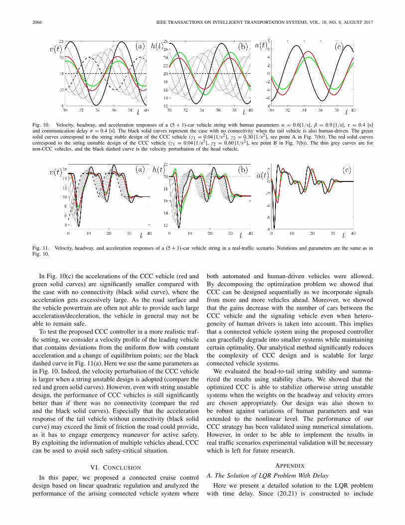
Fig. 10. Velocity, headway, and acceleration responses of a (5 + 1)-car vehicle string with human parameters α = 0.6[1/s], β = 0.9 [1/s], τ = 0.4 [s]and communication delay σ = 0.4 [s]. The black solid curves represent the case with no connectivity when the tail vehicle is also human-driven. The greensolid curves correspond to the string stable design of the CCC vehicle (γ1 = 0.04 [1/s2], γ2 = 0.30 [1/s2], see point A in Fig. 7(b)). The red solid curvescorrespond to the string unstable design of the CCC vehicle (γ1 = 0.04 [1/s2], γ2 = 0.60 [1/s2], see point B in Fig. 7(b)). The thin grey curves are fornon-CCC vehicles, and the black dashed curve is the velocity perturbation of the head vehicle.

Fig. 11. Velocity, headway, and acceleration responses of a (5 + 1)-car vehicle string in a real-traffic scenario. Notations and parameters are the same as inFig. 10.

In Fig. 10(c) the accelerations of the CCC vehicle (red andgreen solid curves) are significantly smaller compared withthe case with no connectivity (black solid curve), where theacceleration gets excessively large. As the road surface andthe vehicle powertrain are often not able to provide such largeacceleration/deceleration, the vehicle in general may not beable to remain safe.

To test the proposed CCC controller in a more realistic traf-fic setting, we consider a velocity profile of the leading vehiclethat contains deviations from the uniform flow with constantacceleration and a change of equilibrium points; see the blackdashed curve in Fig. 11(a). Here we use the same parameters asin Fig. 10. Indeed, the velocity perturbation of the CCC vehicleis larger when a string unstable design is adopted (compare thered and green solid curves). However, even with string unstabledesign, the performance of CCC vehicles is still significantlybetter than if there was no connectivity (compare the redand the black solid curves). Especially that the accelerationresponse of the tail vehicle without connectivity (black solidcurve) may exceed the limit of friction the road could provide,as it has to engage emergency maneuver for active safety.By exploiting the information of multiple vehicles ahead, CCCcan be used to avoid such safety-critical situation.

VI. CONCLUSION

In this paper, we proposed a connected cruise controldesign based on linear quadratic regulation and analyzed theperformance of the arising connected vehicle system where

both automated and human-driven vehicles were allowed.By decomposing the optimization problem we showed thatCCC can be designed sequentially as we incorporate signalsfrom more and more vehicles ahead. Moreover, we showedthat the gains decrease with the number of cars between theCCC vehicle and the signaling vehicle even when hetero-geneity of human drivers is taken into account. This impliesthat a connected vehicle system using the proposed controllercan gracefully degrade into smaller systems while maintainingcertain optimality. Our analytical method significantly reducesthe complexity of CCC design and is scalable for largeconnected vehicle systems.

We evaluated the head-to-tail string stability and summa-rized the results using stability charts. We showed that theoptimized CCC is able to stabilize otherwise string unstablesystems when the weights on the headway and velocity errorsare chosen appropriately. Our design was also shown tobe robust against variations of human parameters and wasextended to the nonlinear level. The performance of ourCCC strategy has been validated using numerical simulations.However, in order to be able to implement the results inreal traffic scenarios experimental validation will be necessarywhich is left for future research.

APPENDIX

A. The Solution of LQR Problem With Delay

Here we present a detailed solution to the LQR problemwith time delay. Since (20,21) is constructed to include


disturbance φ(t) in the LQR format, and the optimal con-troller (27) is given using partitioned matrices (26), we write(24,25) into four groups, where P1(t), Q1(t, θ), R1(t, ξ, θ)are independent from the disturbance and can be solved usingonly the coefficient matrices A,B,D and the weighting factor�. That is, for the first group we obtain the PDE

−P1(t) = ATP1(t)+ P1(t)A − P1(t)DDTP1(t)

+ Q1(t, 0)+ QT1 (t, 0)+ � ,

(∂θ − ∂t )Q1(t, θ) = (AT−P1(t)DDT)

Q1(t, θ)+R1(t, 0, θ),

(∂ξ + ∂θ − ∂t )R1(t, ξ, θ) = −QT1 (t, ξ)DDTQ1(t, θ) , (65)


P1(tf) = 0 ,

Q1(tf , θ) = 0 , Q1(t,−τ ) = P1(t)B ,

R1(tf , ξ, θ) = 0 , R1(t,−τ, θ) = BTQ1(t, θ) . (66)

Using P1(t) and Q1(t, θ) obtained from (65,66), we cancalculate Q2(t, θ) and R2(t, ξ, θ) by solving

(∂θ − ∂t )Q2(t, θ) = (AT−P1(t)DDT)

Q2(t, θ)+R2(t, 0, θ),

(∂t − ∂ξ − ∂θ )R2(t, ξ, θ) = QT1 (t, ξ)DDTQ2(t, θ) , (67)


Q2(tf , θ) = 0 , Q2(t,−τ ) = 0 ,

R2(tf , ξ, θ) = 0 , R2(t,−τ, θ) = BTQ2(t, θ) . (68)

Note that the disturbance φ(t) does not appear in (67) either.As a matter of fact, (67,68) result in Q2(t, θ) ≡ 0 andR2(t, ξ, θ) ≡ 0.

The dynamics of P2(t) and Q3(t, θ) are driven by thedisturbance φ(t):

−P2(t) = (AT − P1(t)DDT)

P2(t)+ P1(t)φ(t)

+ Q2(t, 0)+ QT3 (t, 0) ,

(∂θ−∂t)Q3(t, θ)=(φT(t)−PT

2 (t)DDT)Q1(t, θ)+RT

2 (t, θ, 0),

(69)


P2(tf) = 0 ,

Q3(tf , θ) = 0 , Q3(t,−τ ) = PT2 (t)B . (70)

Although P4(t), Q4(t, θ), R4(t, ξ, θ) do not appear in theoptimal control (27), they appear in the minimal cost function,and are given by the PDE

−P4(t) = φT(t)P2(t)+ P3(t)φ(t) − P3(t)DDTP2(t)

+ Q4(t, 0)+ QT4 (t, 0) ,

(∂θ − ∂t )Q4(t, θ) = (φT(t)−P3(t)DDT)

Q2(t, θ)

+ R4(t, 0, θ),

(∂ξ + ∂θ − ∂t )R4(t, ξ, θ) = −QT2 (t, ξ)DDTQ2(t, θ) , (71)


P4(tf) = 0 ,

Q4(tf , θ) = 0 , Q4(t,−τ ) = 0 ,

R4(tf , ξ, θ) = 0 , R4(t,−τ, θ) = 0 . (72)

B. The Distribution Kernels

Here we provide the constants that appear in the expressionof fi (θ), gi(θ), i = 1, . . . , n in (50) using (44,48,52). Fori = 1 (52) corresponds to

a10 = a11 = a12 = 0, b10 = b11 = b12 = 0 . (73)

For i = 2, . . . , n we write in (44) that

eA1(θ+τ ) = KeJ1(θ+τ )K−1 , (74)

where the Jordan form J1 contains the eigenvalues of A1:

λ1,2 = 1

2

(−

√γ1+γ2+2N∗√γ1 ±

√γ1+γ2−2N∗√γ1

),

(75)

and the real part of λ1, λ2 are smaller than zero (which isensured by the closed-loop plant stability of LQ design). Inmost cases A1 is diagonalizable, that is, J1 = diag([λ1, λ2]).In the special case γ2 = 2N∗√γ1 − γ1, we have λ1 = λ2 andA1 may not be diagonalizable, yielding the nontrivial Jordan

form J1 =[λ1 10 λ1

].

Denote K =[

k11 k12k21 k22

], K−1 =

[i11 i12i21 i22

], then from (44,48)

we obtain[

fi (θ) gi (θ)] = [

fc(θ) gc(θ)](

P1i B1 + P1(i−1)B2), (76)

where

fc(θ) = (tca + tcc(θ + τ )

)eλ1(θ+τ ) + tcbeλ2(θ+τ ) ,

gc(θ) = (sca + scc(θ + τ )

)eλ1(θ+τ ) + scbeλ2(θ+τ ) , (77)

such that we have

tca = (k11 + k21)i11 , tcb = (k12 + k22)i21 ,

sca = (k11 + k21)i12 , scb = (k12 + k22)i22 ,

tcc ={

0 , if A1 is diagonalizable ,

(k11 + k21)i21 , if A1 is not diagonalizable ,

scc ={

0 , if A1 is diagonalizable ,

(k11 + k21)i22 , if A1 is not diagonalizable .

(78)

Substituting (17,77) into (76), we obtain (50) with the coeffi-cients

ai0 = α(tcali1 + scali2) , bi0 = β(tcali1 + scali2) ,

ai1 = α(tccli1 + sccli2) , bi1 = β(tccli1 + sccli2) ,

ai2 = α(tcbli1 + scbli2) , bi2 = β(tcbli1 + scbli2) , (79)

where

li1 = −P1i [1, 1] − P1i [1, 2] + P1(i−1)[1, 2] ,li2 = −P1i [2, 1] − P1i [2, 2] + P1(i−1)[2, 2] , (80)

for i = 2, . . . , n, and C[i, j ] stands for the element of C atthe i th row and j th column.


C. The Contracting Map

To show that the feedback gains and distribution functionsdecay exponentially with the car number, all eigenvalues ofM must be smaller than 1 in magnitude, cf. (46,47).

We assume diagonalizable A1 and plug (74) into (47) toobtain

M = (I ⊗ K)M(I ⊗ K−1) , (81)

where

M =−[

J1 − αeτ J1 −αeτ J1

N∗I − βeτ J1 J1 − βeτ J1

]−1[0 αeτ J1

0 βeτ J1

]

. (82)

Indeed, the eigenvalues of M are the same as the eigenvaluesof M. It is evident that M has two zero eigenvalues, while theother two non-zero eigenvalues are

μ1,2 = − αN∗ − βλ1,2

λ21,2e−τλ1,2 − (α + β)λ1,2 + αN∗ , (83)

where λ1,2 are given in (75). That is, the recursive map (46,47)is contracting if

|μ1| < 1, |μ2| < 1 . (84)

Consider plant stable human-driven vehicles where N∗ andα, β are positive. We found that (84) holds in the stringstable region in the parameter space. Note that (83) bears aninteresting resemblance to H0(s) in (55), and still holds whenA1 is not diagonalizable.

D. Robustness of CCC Against Other CCC Vehicles

Here we consider the scenario where vehicles 2 − n inFig. 2 are no longer homogeneous, that is, some of themmay have different human parameters or even become CCCvehicles. To demonstrate the general influence of heterogeneityamong preceding vehicles on the CCC design, we assume thedynamics of vehicle i is

hi (t) = vi+1(t)− vi (t) ,

vi (t) =n∑

j=i

(αi j

(Vj (h j (t−τ ))−v j (t−τ )

) + βi j h j (t−τ )),

(85)

for i = 2, . . . , n, where αi j , βi j are vehicle i ’s feedback gainson motion signals from vehicle j , cf. (2,64).

Thus, the dynamics of the connected vehicle system is stilldescribed by (15), with a new coefficient matrix

B =

⎡

⎢⎢⎢⎢⎢⎣

0 B12 B13 · · · B1n

B22 B23 · · · B2n. . .

...B(n−1)(n−1) B(n−1)n

Bnn

⎤

⎥⎥⎥⎥⎥⎦, (86)

where

B1i =[

0 0α2i β2i

], Bii = −

[αii βii

αii βii

], i = 2, · · · , n,

Bi j =[ −αi j −βi j

α(i+1) j − αi j β(i+1) j − βi j

], j = i + 1, · · · , n ,

(87)

cf. (16,17).

Fig. 12. The optimized headway and velocity gains α1i , β1i , i = 1, . . . , nof the CCC vehicle in a (10 + 1)-car system for homogeneous (blue crosses)and heterogeneous (green diamonds) human gains as indicated. The otherparameters are the same as in Fig. 4.

Since the matrix B is still upper-triangular, the optimalcontrol design (31,32,34) can be decomposed as before. Nowinstead of (44,46,47), we have

Q1i(θ) =i∑

k=1

eA1(θ+τ )P1kBki , (88)

and

vec(P1i ) =i−1∑

k=1

Mikvec(P1k), (89)

for i = 2, . . . , n, where

Mik = −(I ⊗ A1 + AT1 ⊗ I + BT

ii ⊗ eτ A1)−1(BTki ⊗ eτ A1).

(90)

This means that the maps between vec(P1i ), i = 2, . . . , n, andvec(P11) are determined by Bki , k = 2, . . . , i − 1, i.e., by theconnectivity structure between vehicle 1 and vehicle i . Thus,the connectivity structure among vehicles farther downstreamstill does not influence feedback gains on existing feedbackterms of the CCC controller.

We first demonstrate only the influence of heterogeneoushuman parameters. In this case, the coefficient matrix B stillhas the same structure is in (16), i.e., Bi j �= 0 only for j =i + 1. Thus, there is only one term Mi(i−1) left in the right-hand side of (89), and it still defines a recursively contractingmap given plant stable human parameters in (90).

As an example, we take a (10 + 1)-car connected system,keep the design parameters γ1 = 0.04 [1/s2], γ2 = 0.30 [1/s2]and human reaction time τ = 0.4 [s] as in Fig. 4, butincrease/decrease the human gains for vehicles 2, 3, 4, 5 asindicated in Fig. 12. The blue crosses correspond to thehomogeneous system (cf. Fig. 4), while the green diamondscorrespond to the heterogeneous system. The gains α11, β11are the same for both cases, because they do not dependon parameters of preceding vehicles. Although α1i , β1i ,i = 2, . . . , n differ between the homogeneous and hetero-geneous cases, the difference is only noticeable for i = 2, 3,even though α44, β44, α55, β55 differ significantly. This isbecause the contracting map (89,90) forces the gains to


Fig. 13. The optimized headway and velocity gains α1i , β1i , i = 2, . . . , n ofthe CCC vehicle in a (10+1)-car connected vehicle system. The blue crossesdenote gains obtained with homogeneous human-driven vehicles, while thegreen squares denote the case when vehicle 3 uses additional feedback fromvehicle 5, with gains α35 = 0.9 [1/s] and β35 = 0.9 [1/s]. The otherparameters are the same as in Fig. 4.

decrease for signals coming from farther downstream, andthen heterogeneity of vehicles further away has less significantimpact on the CCC vehicle.

We then consider the robustness of the CCC design againstextra connectivity links among preceding vehicles. In Fig. 13,the blue crosses still show the gains in a (10 + 1)-car systemwith homogeneous human-driven vehicles (cf. Fig. 4), whilethe green squares depict the case when vehicle 3 is also usingmotion information of vehicle 5, with feedback gainsα35 = 0.6 [1/s] and β35 = 0.9 [1/s]. Notice that the gainsα1i , β1i of the CCC controller do not change for i = 1, . . . , 4.While α15 and β15 change considerably, as i increases furtherthe changes in α1i , β1i decay exponentially. These case studiesdemonstrate that our proposed algorithm is robust againstheterogeneity among preceding vehicles.

REFERENCES

[1] D. Schrank, B. Eisele, and T. Lomax, “TTI’s 2012 urban mobilityreport,” Texas A&M Transp. Inst. and Texas A&M Univ. Syst., CollegeStation, TX, USA, 2012.

[2] K. Li and P. Ioannou, “Modeling of traffic flow of automated vehicles,”IEEE Trans. Intell. Transp. Syst., vol. 5, no. 2, pp. 99–113, Jun. 2004.

[3] L. C. Davis, “Effect of adaptive cruise control systems on traffic flow,”Phys. Rev. E, vol. 69, no. 6, p. 066110, Jun. 2004.

[4] X. Cheng, L. Yang, and X. Shen, “D2D for intelligent transportationsystems: A feasibility study,” IEEE Trans. Intell. Transp. Syst., vol. 16,no. 4, pp. 1784–1793, Aug. 2015.

[5] X. Cheng et al., “Electrified vehicles and the smart grid: TheITS perspective,” IEEE Trans. Intell. Transp. Syst., vol. 15, no. 4,pp. 1388–1404, Aug. 2014.

[6] E. V. Nunen, M. R. J. A. E. Kwakkernaat, J. Ploeg, andB. D. Netten, “Cooperative competition for future mobility,” IEEE Trans.Intell. Transp. Syst., vol. 13, no. 3, pp. 1018–1025, Sep. 2012.

[7] E. Chan, P. Gilhead, P. Jelínek, P. Krejcí, and T. Robinson, “Cooperativecontrol of SARTRE automated platoon vehicles,” in Proc. 19th ITSWorld Congr., 2012, pp. 22–26.

[8] B. van Arem, C. J. G. van Driel, and R. Visser, “The impact ofcooperative adaptive cruise control on traffic-flow characteristics,” IEEETrans. Intell. Transp. Syst., vol. 7, no. 4, pp. 429–436, Dec. 2006.

[9] M. di Bernardo, A. Salvi, and S. Santini, “Distributed consensus strategyfor platooning of vehicles in the presence of time-varying heterogeneouscommunication delays,” IEEE Trans. Intell. Transp. Syst., vol. 16, no. 1,pp. 102–112, Feb. 2015.

[10] V. Milanes, J. Alonso, L. Bouraoui, and J. Ploeg, “Cooperative maneu-vering in close environments among cybercars and dual-mode cars,”IEEE Trans. Intell. Transp. Syst., vol. 12, no. 1, pp. 15–24, Mar. 2011.

[11] J. Ploeg, N. van de Wouw, and H. Nijmeijer, “Lp string stabilityof cascaded systems: Application to vehicle platooning,” IEEE Trans.Control Syst. Technol., vol. 22, no. 2, pp. 786–793, Mar. 2014.

[12] J. Ploeg, E. Semsar-Kazerooni, G. Lijster, N. van de Wouw, andH. Nijmeijer, “Graceful degradation of cooperative adaptive cruisecontrol,” IEEE Trans. Intell. Transp. Syst., vol. 16, no. 1, pp. 488–497,Feb. 2015.

[13] J. Ploeg, D. P. Shukla, N. van de Wouw, and H. Nijmeijer, “Controllersynthesis for string stability of vehicle platoons,” IEEE Trans. Intell.Transp. Syst., vol. 15, no. 2, pp. 845–865, Apr. 2014.

[14] M. Wang, W. Daamen, S. P. Hoogendoorn, and B. van Arem, “Rollinghorizon control framework for driver assistance systems. Part II: Coop-erative sensing and cooperative control,” Transp. Res. C, vol. 40,pp. 290–311, Mar. 2014.

[15] Y. Zheng, S. E. Li, J. Wang, D. Cao, and K. Li, “Stability and scalabilityof homogeneous vehicular platoon: Study on the influence of informa-tion flow topologies,” IEEE Trans. Intell. Transp. Syst., vol. 17, no. 1,pp. 14–26, Jan. 2016.

[16] G. Orosz, “Connected cruise control: Modelling, delay effects, andnonlinear behaviour,” Vehicle Syst. Dyn., vol. 54, no. 8, pp. 1147–1176,2016.

[17] L. Zhang and G. Orosz, “Motif-based design for connected vehiclesystems in presence of heterogeneous connectivity structures and timedelays,” IEEE Trans. Intell. Transp. Syst., vol. 17, no. 6, pp. 1638–1651,Jun. 2016.

[18] G. Orosz, R. E. Wilson, and G. Stépán, “Traffic jams: Dynamics andcontrol,” Philos. Trans. Roy. Soc. A, vol. 368, no. 1928, pp. 4455–4479,2010.

[19] J. I. Ge and G. Orosz, “Dynamics of connected vehicle systems withdelayed acceleration feedback,” Transp. Res. C, Emerg. Technol., vol. 46,pp. 46–64, Sep. 2014.

[20] W. B. Qin, M. M. Gomez, and G. Orosz, “Stability and frequencyresponse under stochastic communication delays with applications toconnected cruise control design,” IEEE Trans. Intell. Transp. Syst.,vol. PP, no. 99, pp. 1–16. [Online]. Available: http://dx.doi.org/10.1109/TITS.2016.2574246

[21] S. S. Avedisov and G. Orosz, “Nonlinear network modes in cyclicsystems with applications to connected vehicles,” J. Nonlinear Sci.,vol. 25, no. 4, pp. 1015–1049, Aug. 2015.

[22] J. I. Ge and G. Orosz, “Optimal control of connected vehicle systems,”in Proc. 53rd IEEE Conf. Decision Control, Dec. 2014, pp. 4107–4112.

[23] D. Helbing, “Traffic and related self-driven many-particle systems,” Rev.Mod. Phys., vol. 73, no. 4, pp. 1067–1141, 2001.

[24] K. Nagel, P. Wagner, and R. Woesler, “Still flowing: Approaches totraffic flow and traffic jam modeling,” Oper. Res., vol. 51, no. 5,pp. 681–710, 2003.

[25] M. Treiber, A. Hennecke, and D. Helbing, “Congested traffic statesin empirical observations and microscopic simulations,” Phys. Rev. E,vol. 62, no. 2, pp. 1805–1824, 2000.

[26] M. Bando, K. Hasebe, A. Nakayama, A. Shibata, and Y. Sugiyama,“Dynamical model of traffic congestion and numerical simulation,” Phys.Rev. E, vol. 51, pp. 1035–1042, Feb. 1995.

[27] R. Herman, E. W. Montroll, R. B. Potts, and R. W. Rothery, “Trafficdynamics: Analysis of stability in car following,” Oper. Res., vol. 7,no. 1, pp. 86–106, 1959.

[28] D. C. Gazis, R. Herman, and R. W. Rothery, “Nonlinear follow-the-leader models of traffic flow,” Oper. Res., vol. 9, no. 4, p. 545–567,1961.

[29] P. A. Ioannou and M. Stefanovic, “Evaluation of ACC vehicles in mixedtraffic: Lane change effects and sensitivity analysis,” IEEE Trans. Intell.Transp. Syst., vol. 6, no. 1, pp. 79–89, Mar. 2005.

[30] S. Krauss, P. Wagner, and C. Gawron, “Metastable states in a micro-scopic model of traffic flow,” Phys. Rev. E, vol. 55, no. 5, pp. 5597–5602,1997.

[31] R. Wiedemann, Simulation des Strassenverkehrsflusses (Institut FurVerkehrswesen Der). Karlsruhe, Germany: Univ. Karlsruhe, 1973.

[32] D. Krajzewicz, J. Erdmann, M. Behrisch, and L. Bieker, “Recentdevelopment and applications of SUMO—Simulation of urban mobility,”Int. J. Adv. Syst. Meas., vol. 5, nos. 3–4, pp. 128–138, 2012.

[33] Q. Yang and H. N. Koutsopoulos, “A microscopic traffic simulator forevaluation of dynamic traffic management systems,” Transp. Res. C,Emerg. Technol., vol. 4, no. 3, pp. 113–129, Jun. 1996.

[34] S. Hoogendoorn and R. Hoogendoorn, “Calibration of microscopictraffic-flow models using multiple data sources,” Philos. Trans. Roy. Soc.London A, Math. Phys. Sci., vol. 368, no. 1928, pp. 4497–4517, 2010.

[35] P. Wagner, “Fluid-dynamical and microscopic description of traffic flow:A data-driven comparison,” Philos. Trans. Roy. Soc. London A, Math.Phys. Sci., vol. 368, no. 1928, pp. 4481–4495, 2010.


[36] P. Seiler, A. Pant, and K. Hedrick, “Disturbance propagation in vehiclestrings,” IEEE Trans. Autom. Control, vol. 49, no. 10, pp. 1835–1842,Oct. 2004.

[37] C. R. He, H. Maurer, and G. Orosz, “Fuel consumption optimizationof heavy-duty vehicles with grade, wind, and traffic information,”J. Comput. Nonlinear Dyn., vol. 11, no. 6, p. 061011-1–061011-12,2016.

[38] V. Kolmanovskii and A. Myshkis, Applied Theory of Functional Differ-ential Equations. Norwell, MA, USA: Kluwer, 1992.

[39] D. W. Ross and I. Flügge-Lotz, “An optimal control problem for systemswith differential-difference equation dynamics,” J. Control, vol. 7, no. 4,pp. 609–623, 1969.

[40] F. Bai and H. Krishnan, “Reliability analysis of DSRC wireless commu-nication for vehicle safety applications,” in Proc. IEEE Intell. Transp.Syst. Conf., Sep. 2006, pp. 355–362.

Jin I. Ge received the bachelor’s degree in trans-portation engineering and the master’s degree inautomotive engineering from Beijing University ofAeronautics and Astronautics, China, in 2010 and2012, respectively. She is currently working towardthe Ph.D. degree in mechanical engineering withUniversity of Michigan, Ann Arbor. Her researchfocuses on dynamics and control of connected vehi-cles, optimal control, and time delay systems.

Gábor Orosz received the M.Sc. degree in engi-neering physics from Budapest University of Tech-nology and Economics, Hungary, in 2002 and thePh.D. degree in engineering mathematics from Uni-versity of Bristol in 2006. He held postdoctoralpositions with University of Exeter and University ofCalifornia, Santa Barbara. He has been an AssistantProfessor in mechanical engineering with Universityof Michigan, Ann Arbor, since 2010. His researchfocuses on nonlinear dynamics and control, timedelay systems, networks and complex systems with

applications on connected and automated vehicles, and biological networks.

2056 IEEE TRANSACTIONS ON INTELLIGENT …orosz/articles/ITS_2017_Jin.pdf · GE AND OROSZ: OPTIMAL...

Documents

Transcript of 2056 IEEE TRANSACTIONS ON INTELLIGENT …orosz/articles/ITS_2017_Jin.pdf · GE AND OROSZ: OPTIMAL...