Basic Electrical Engineering · 2020. 12. 23. · Basic Electrical Engineering

DEPARTMENT
OF
ELECTRICAL AND ELECTRONICS ENGINEERING
III BTECH I SEMESTER
REGULATIONLAB CODE R16EE506PC
LABORATORY MANUAL
BASIC ELECTRICAL SIMULATION
Basic Electrical Simulation Lab
Department of Electrical amp Electronics Engineering
DEPARTMENT VISION
To become a renowned department imparting both technical and non-technical skills to the
students by implementing new engineering pedagogyrsquos and research to produce competent new
age electrical engineers
DEPARTMENT MISSION
To transform the students into motivated and knowledgeable new age electrical engineers
To advance the quality of education to produce world class technocrats with an ability to adapt
to the academically challenging environment
To provide a progressive environment for learning through organized teaching methodologies
contemporary curriculum and research in the thrust areas of electrical engineering
Basic Electrical Simulation Lab
Department of Electrical amp Electronics Engineering
Program Educational Objectives (PEOrsquos)
PEO 1 Apply knowledge and skills to provide solutions to Electrical and Electronics
Engineering problems in industry and governmental organizations or to enhance student learning
in educational institutions
PEO 2 Work as a team with a sense of ethics and professionalism and communicate
effectively to manage cross-cultural and multidisciplinary teams
PEO 3 Update their knowledge continuously through lifelong learning that contributes to
personal global and organizational growth
Basic Electrical Simulation Lab
Department of Electrical amp Electronics Engineering
Program Outcomes(POrsquos)
A graduate of the Electrical and Electronics Engineering Program will demonstrate
PO 1 Engineering knowledge Apply the knowledge of mathematics science engineering
fundamentals and an engineering specialization to the solution of complex engineering
problems
PO 2 Problem analysis Identify formulate review research literature and analyze complex
engineering problems reaching substantiated conclusions using first principles of mathematics
natural science and engineering sciences
PO 3 Designdevelopment of solutions design solutions for complex engineering problems
and design system components or processes that meet the specified needs with appropriate
consideration for the public health and safety and the cultural societal and environmental
considerations
PO 4 Conduct investigations of complex problems use research based knowledge and
research methods including design of experiments analysis and interpretation of data and
synthesis of the information to provide valid conclusions
PO 5 Modern tool usage create select and apply appropriate techniques resources and
modern engineering and IT tools including prediction and modelling to complex engineering
activities with an understanding of the limitations
PO 6 The engineer and society apply reasoning informed by the contextual knowledge to
assess societal health safety legal and cultural issues and the consequent responsibilities
relevant to the professional engineering practice
PO 7 Environment sustainability understand the impact of the professional engineering
solutions in the societal and environmental contexts and demonstrate the knowledge of and
need for sustainable development
PO 8 Ethics apply ethical principles and commit to professional ethics and responsibilities
and norms of the engineering practice
PO 9 Individual and team work function effectively as an individual and as a member or
leader in diverse teams and in multidisciplinary settings
PO 10 Communication communicate effectively on complex engineering activities with the
engineering community and with society at large such as being able to comprehend and write
effective reports and design documentation make effective presentations and give and receive
clear instructions
PO 11 Project management and finance demonstrate knowledge and understanding of the
engineering and management principles and apply these to onersquos own work as a member and
leader in a team to manage projects and in multidisciplinary environments
PO 12 Lifelong learning recognize the need for and have the preparation and ability to
engage in independent and lifelong learning in the broader context of technological change
Basic Electrical Simulation Lab
Department of Electrical amp Electronics Engineering
Program Specific Outcomes(PSOrsquos)
PSO-1 Apply the engineering fundamental knowledge to identify formulate design and
investigate complex engineering problems of electric circuits power electronics electrical
machines and power systems and to succeed in competitive exams like GATE IES GRE OEFL
GMAT etc
PSO-2 Apply appropriate techniques and modern engineering hardware and software tools in
power systems and power electronics to engage in life-long learning and to get an employment in
the field of Electrical and Electronics Engineering
PSO-3 Understand the impact of engineering solutions in societal and environmental context
commit to professional ethics and communicate effectively
Basic Electrical Simulation Lab
Department of Electrical amp Electronics Engineering
Course Outcomes (COrsquos)
Upon completion of this course the student will be able to
CO1 Analyze signal generation in different systems
CO2 Analyze network by various techniques
CO3 Analyze circuit responses
CO4 Analyze bridge rectifiers
Basic Electrical Simulation Lab
Department of Electrical amp Electronics Engineering
EE506PC BASIC ELECTRICAL SIMULATION LAB
BTech III Year II Sem L T P C
0 0 3 2
Note Minimum 12 experiments should be conducted
Experiments are to be simulated using Multisim or P-spice or Equivalent Simulation and
then testing to be done in hardware
The following experiments are required to be conducted compulsory experiments
1 Basic Operations on Matrices
2 Generation of various signals and sequences (Periodic and Aperiodic) such as unit Impulse
Step Square Saw tooth Triangular Sinusoidal Ramp Sinc
3 Operations on signals and sequences such as Addition Multiplication Scaling
Shifting Folding Computation of Energy and Average Power
4 Mesh and Nodal Analysis of Electrical circuits
5 Application of Network Theorems to Electrical Networks
6 Waveform Synthesis using Laplace Transform
7 Locating the Zeros and Poles and Plotting the Pole-Zero maps in S plane and Z-Plane for the
given transfer function
8 Harmonic analysis of non sinusoidal waveforms
In addition to the above eight experiments at least any two of the experiments from the
following list are required to be conducted
9 Simulation of DC Circuits
10 Transient Analysis
11 Measurement of active Power of three phase circuit for balanced and unbalanced load
12 Simulation of single phase diode bridge rectifiers with filter for R amp RL load
13 Simulation of three phase diode bridge rectifiers with R RL load
14 Design of Low Pass and High Pass filters
15 Finding the Even and Odd parts of Signal Sequence and Real and imaginary parts of Signal
16 Finding the Fourier Transform of a given signal and plotting its magnitude and phase
spectrum
Basic Electrical Simulation Lab
Department of Electrical amp Electronics Engineering
Instructions to the students
A Dorsquos
1 Attend the laboratory always in time
2 Attend in formal dress
3 Submit the laboratory record and observation in every lab session
4 Use the laboratory systems properly and carefully
5 Attend the lab with procedure for the experiment
6 Switch off the systems immediately after the completion of the experiment
7 Place the bags outside
8 Leave the footwear outside
B Donrsquots
1 Donrsquot make noise in the laboratory
2 Donrsquot miss handle lab system
3 Donrsquot use cell phone in the lab
Basic Electrical Simulation Lab
Department of Electrical amp Electronics Engineering
INTRODUCTION TO SOFTWARE
MATLAB is widely used in all areas of applied mathematics in education and research at
universities and in the industry MATLAB stands for MATrix LABoratory and the software is
built up around vectors and matrices This makes the software particularly useful for linear
algebra but MATLAB is also a great tool for solving algebraic and differential equations and for
numerical integration MATLAB has powerful graphic tools and can produce nice pictures in both
2D and 3D It is also a programming language and is one of the easiest programming languages
for writing mathematical programs MATLAB also has some tool boxes useful for signal
processing image processing optimization etc
The MATLAB environment (on most computer systems) consists of menus buttons and a
writing area similar to an ordinary word processor There are plenty of help functions that you are
encouraged to use The writing area that you will see when you start MATLAB is called
the command window In this window you give the commands to MATLAB For example when
you want to run a program you have written for MATLAB you start the program in the command
window by typing its name at the prompt The command window is also useful if you just want to
use MATLAB as a scientific calculator or as a graphing tool If you write longer programs you
will find it more convenient to write the program code in a separate window and then run it in the
command window
Octave is an open-source interactive software system for numerical computations and
graphics It is particularly designed for matrix computations solving simultaneous equations
computing eigenvectors and Eigen values and so on In many real-world engineering problems the
data can be expressed as matrices and vectors and boil down to these forms of solution In
addition Octave can display data in a variety of different ways and it also has its own
programming language which allows the system to be extended It can be thought of as a very
powerful programmable graphical calculator Octave makes it easy to solve a wide range of
numerical problems allowing you to spend more time experimenting and thinking about the wider
problem Octave was originally developed as a companion software to a undergraduate course
book on chemical reactor design It is currently being developed under the leadership of Dr JW
Eaton and released under the GNU General Public Licence Octaversquos usefulness is enhanced in
that it is mostly syntax compatible with MATLAB which is commonly used in industry and
academia
Basic Electrical Simulation Lab
Department of Electrical amp Electronics Engineering
INDEX
SNo Name of the Experiment Page No
1 Basic Operations on Matrices
2 Generation of various signals and sequences
(Periodic and Aperiodic)
3 Operations on signals and sequences
4 Mesh and Nodal Analysis of Electrical circuits
5 Application of Network Theorems to Electrical
Networks
6 Waveform Synthesis using Laplace Transform
7 Locating the Zeros and Poles and Plotting the Pole-
Zero maps in S plane and Z-Plane for the given
transfer function
8 Harmonic analysis of non sinusoidal waveforms
9 Simulation of DC Circuits
10 Transient Analysis
11 Measurement of active Power of three phase circuit
for balanced and unbalanced load
12 Simulation of single phase diode bridge rectifiers
with filter for R amp RL load
13 Simulation of three phase diode bridge rectifiers
with R RL load
14 Design of Low Pass and High Pass filters
15 Finding the Even and Odd parts of Signal
Sequence and Real and imaginary parts of Signal
16 Finding the Fourier Transform of a given signal and
plotting its magnitude and phase spectrum
Basic Electrical Simulation Lab
Department of Electrical amp Electronics Engineering
EXPERIMENT -1
BASIC OPERATIONS ON MATRICES
AIM To write a OCTAVE program to perform some basic operation on matrices such as
addition subtraction multiplication
APPARATUS
1 OCTAVE
2 LINUX
THEORY
Built in Functions
1 Scalar Functions
Certain OCTAVE functions are essentially used on scalars but operate element-wise when
applied to a matrix (or vector) They are summarized below
1 sin - trigonometric sine
2 cos - trigonometric cosine
3 tan - trigonometric tangent
4 asin - trigonometric inverse sine (arcsine)
5 acos - trigonometric inverse cosine (arccosine)
6 atan - trigonometric inverse tangent (arctangent)
7 exp - exponential
8 log - natural logarithm
9 abs - absolute value
10 sqrt - square root
11 rem - remainder
12 round - round towards nearest integer
13 floor - round towards negative infinity
14 ceil - round towards positive infinity
2 Vector Functions
Other OCTAVE functions operate essentially on vectors returning a scalar value Some of
these functions are given below
1 max largest component get the row in which the maximum element lies
2 min smallest component
3 length length of a vector
4 sort sort in ascending order
Basic Electrical Simulation Lab
Department of Electrical amp Electronics Engineering
5 sum sum of elements
6 prod product of elements
7 median median value
8 mean mean value std standard deviation
3 Matrix Functions
Much of OCTAVE‟ s power comes from its matrix functions These can be further separated
into two sub-categories
The first one consists of convenient matrix building functions some of which are given below
1 eye - identity matrix
2 zeros - matrix of zeros
3 ones - matrix of ones
4 diag - extract diagonal of a matrix or create diagonal matrices
5 triu - upper triangular part of a matrix
6 tril - lower triangular part of a matrix
7 rand - randomly generated matrix
eg diag([090920516302661])
ans =
09092 0 0
0 05163 0
0 0 02661
Commands in the second sub-category of matrix functions are
1 size size of a matrix
2 det determinant of a square matrix
3 inv inverse of a matrix
4 rank rank of a matrix
5 rref reduced row echelon form
6 eig eigenvalues and eigenvectors
7 poly characteristic polynomial
Basic Electrical Simulation Lab
Department of Electrical amp Electronics Engineering
PROGRAM-
clc
close all
clear all
a=[1 2 -9 2 -1 2 3 -4 3]
b=[1 2 3 4 5 6 7 8 9]
disp(The matrix a= )
a
disp(The matrix b= )
b
to find sum of a and b
c=a+b
disp(The sum of a and b is )
c
to find difference of a and b
d=a-b
disp(The difference of a and b is )
d
to find multiplication of a and b
e=ab
disp(The product of a and b is )
e
end
PROCEDURE-
1 Open OCTAVE
2 Open new script
3 Type the program
4 Save in current directory
5 Compile and Run the program
6 For the output see command window Figure window
OUTPUT-
Basic Electrical Simulation Lab
Department of Electrical amp Electronics Engineering
RESULT-
EXPERIMENT -2
GENERATION OF VARIOUS SIGNALS AND SEQUENCES (PERIODIC AND
APERIODIC) SUCH AS UNIT IMPULSE STEP SQUARE SAW TOOTH
TRIANGULAR SINUSOIDAL RAMP SINC
AIM To write a ldquoOCTAVErdquo Program to generate various signals and sequences such as
Unit impulse unit step unit ramp sinusoidal square saw tooth triangular sinc signals
APPARATUS
1 OCTAVE
2 LINUX
THEORY
One of the more useful functions in the study of linear systems is the unit impulse function
An ideal impulse function is a function that is zero everywhere but at the origin where it is
infinitely high However the area of the impulse is finite This is at first hard to visualize but
we can do so by using the graphs shown below
Basic Electrical Simulation Lab
Department of Electrical amp Electronics Engineering
Unit Step Function
The unit step function and the impulse function are considered to be fundamental functions in
Engineering and it is strongly recommended that the reader becomes very familiar with both of
these functions
The unit step function also known as the Heaviside function is defined as such
Sometimes u(0) is given other values usually either 0 or 1 For many applications it is irrelevant
what the value at zero is u(0) is generally written as undefined
Sinc Function
There is a particular form that appears so frequently in communications engineering that we give
it its own name This function is called the Sinc function The Sinc function is defined in the
following manner
And Sinc(0)=1
The value of sinc(x) is defined as 1 at x = 0 since
Then since cos(0) = 1 we can apply the Squeeze Theorem to show that the sinc function
approaches one as x goes to zero Thus defining sinc(0) to be 1 makes the sinc function
continuous Also the Sinc function approaches zero as x goes towards infinity with the envelope
of sinc(x) tapering off as 1x
Basic Electrical Simulation Lab
Department of Electrical amp Electronics Engineering
Rect Function
The Rect Function is a function which produces a rectangular shaped pulse with a width of 1
centred at t = 0 The Rect function pulse also has a height of 1 The Sinc function and the
rectangular function form a Fourier transform pair
A Rect function can be written in the form
where the pulse is centered at X and has width Y We can define the impulse function above in
terms of the rectangle function by centering the pulse at zero (X = 0) setting its height to 1A and
setting the pulse width to A which approaches zero
We can also construct a Rect function out of a pair of unit step functions
Here both unit step functions are set a distance of Y2 away from the center point of (t - X)
SAW TOOTH-
The sawtooth wave (or saw wave) is a kind of non-sinusoidal waveform It is named a sawtooth
based on its resemblance to the teeth on the blade of a saw The convention is that a sawtooth
wave ramps upward and then sharply drops However there are also sawtooth waves in which the
wave ramps downward and then sharply rises The latter type of sawtooth wave is called a reverse
sawtooth wave or inverse sawtooth wave As audio signals the two orientations of sawtooth
wave sound identical The piecewise linear function based on the floor function of time t is an
example of a sawtooth wave with period 1
TRIANGLE WAVE
A triangle wave is a non-sinusoidal waveform named for its triangular shape A band
limited triangle wave pictured in the time domain (top) and frequency domain (bottom) The
fundamental is at 220 Hz (A2)Like a square wave the triangle wave contains only odd
harmonics However the higher harmonics roll off much faster than in a square wave
(proportional to the inverse square of the harmonic number as opposed to just the inverse)It is
possible to approximate a triangle wave with additive synthesis by adding odd harmonics of the
fundamental multiplying every (4n-1)th harmonic by -1and rolling off the harmonics by
the inverse square of their relative frequency to the undamental This infinite Fourier series
converges to the triangle
Basic Electrical Simulation Lab
Department of Electrical amp Electronics Engineering
SINUSOIDAL SIGNAL GENERATION
The sine wave or sinusoid is a mathematical function that describes a smooth repetitive
oscillation It occurs often in pure mathematics as well as physics signal processing electrical
engineering and many other fields Its most basic form as a function of time (t) is
where
bull A the amplitude is the peak deviation of the function from its center position
bull the angular frequency specifies how many oscillations occur in a unit time interval in
radians per second
bull the phase specifies where in its cycle the oscillation begins at t = 0
PROGRAM-
impulse
clc
clear all
close all
t=-10110
x=(t==0)
subplot(211)
plot(txb)
xlabel(time)
ylabel(amplitude)
title(unit impulse function)
subplot(212)
stem(txr)
xlabel(time)
ylabel(amplitude)
title(unit impulse discrete function)
Basic Electrical Simulation Lab
Department of Electrical amp Electronics Engineering
Step
clc
clear all
close all
N=100
t=1100
x=ones(1N)
subplot(211)
plot(txr)
xlabel(time)
ylabel(amplitude)
title(unit step function)
subplot(212)
stem(txr)
xlabel(time)
ylabel(amplitude)
title(unit step discrete function)
Ramp
clc
clear all
close all
t=020
x=t
subplot(211)
plot(txr)
xlabel(time)
ylabel(amplitude)
title(unit ramp function)
subplot(212)
stem(txr)
xlabel(time)
ylabel(amplitude)
title(unit ramp discrete function)
Basic Electrical Simulation Lab
Department of Electrical amp Electronics Engineering
Sinusoidal
clc
clear all
close all
t=0000012
x=sin(2pit)
subplot(211)
plot(txr)
xlabel(time)
ylabel(amplitude)
title(sinusoidal signal)
subplot(212)
stem(txr)
xlabel(time)
ylabel(amplitude)
title(sinusoidal sequence)
Square
clc
clear all
close all
t=00012
x=square(2pit)
subplot(211)
plot(txr)
xlabel(time)
ylabel(amplitude)
title(square signal)
subplot(212)
stem(txr)
xlabel(time)
ylabel(amplitude)
title(square sequence)
Basic Electrical Simulation Lab
Department of Electrical amp Electronics Engineering
Sawtooth
clc
clear all
close all
t=00012
x=sawtooth(2pi5t)
subplot(211)
plot(txk)
xlabel(time)
ylabel(amplitude)
title(sawtooth signal)
subplot(212)
stem(txr)
xlabel(time)
ylabel(amplitude)
title(sawtooth sequence)
Traingular
clc
clear all
close all
t=00012
x=sawtooth(2pi5t05)
subplot(211)
plot(txk)
xlabel(time)
ylabel(amplitude)
title(triangular signal)
subplot(212)
stem(txr)
xlabel(time)
ylabel(amplitude)
title(triangular sequence)
Basic Electrical Simulation Lab
Department of Electrical amp Electronics Engineering
Sinc
clc
clear all
close all
t=linspace(-55)
x=sinc(t)
subplot(211)
plot(txk)
xlabel(time)
ylabel(amplitude)
title(sinc signal)
subplot(212)
stem(txr)
xlabel(time)
ylabel(amplitude)
title(sinc sequence)
PROCEDURE-
1 Open OCTAVE
2 Open new script
3 Type the program
4 Save in current directory
5 Compile and Run the program
6 For the output see command window Figure window
OUTPUT-
RESULT-
Basic Electrical Simulation Lab
Department of Electrical amp Electronics Engineering
EXPERIMENT-3
OPERATIONS ON SIGNALS AND SEQUENCES SUCH AS ADDITION
MULTIPLICATION SCALING SHIFTING FOLDING COMPUTATION OF ENERGY
AND AVERAGE POWER
AIM To performs operations on signals and sequences such as addition multiplication
scaling shifting folding computation of energy and average power
APPARATUS
1 OCTAVE
2 LINUX
THEORY
Basic Operation on Signals
Time shifting y(t)=x(t-T)The effect that a time shift has on the appearance of a signal If T is a
positive number the time shifted signal x (t -T ) gets shifted to the right otherwise it gets shifted
left
Signal Shifting and Delay
Shifting y(n)=x(n-k) m=n-k y=x
Time reversal Y(t)=y(-t) Time reversal _ips the signal about t = 0 as seen in Figure
Signal Addition and Substraction
Addition any two signals can be added to form a third signal z (t) = x (t) + y (t)
Signal AmplificationAttuation
Basic Electrical Simulation Lab
Department of Electrical amp Electronics Engineering
MultiplicationDivition
Multiplication of two signals their product is also a signal z (t) = x (t) y (t)
folding
y(n)=x(-n) y=fliplr(x) n=-fliplr(n)
PROGRAM-
Addition and multiplication of two signals
clc
clear all
close all
t=000012
s1=6sin(2pi5t)
subplot(411)
plot(ts1g)
xlabel(time)
ylabel(amplitude)
title(first signal)
s2=8sin(2pi5t)
subplot(412)
plot(ts2r)
xlabel(time)
ylabel(amplitude)
title(second signal)
s3=s1+s2
subplot(413)
plot(ts3g)
xlabel(time)
ylabel(amplitude)
title(sum of two signals)
s4=s1s2
subplot(414)
plot(ts4g)
xlabel(time)
ylabel(amplitude)
title(multiplication of two signals)
Basic Electrical Simulation Lab
Department of Electrical amp Electronics Engineering
Amplitude scaling for signals
clc
clear all
close all
t=000012
s1=6sin(2pi5t)
subplot(311)
plot(ts1g)
xlabel(time)
ylabel(amplitude)
title(sinusoidal signal)
s2=3s1
subplot(312)
plot(ts2r)
xlabel(time)
ylabel(amplitude)
title(amplified signal)
s3=s13
subplot(313)
plot(ts3g)
xlabel(time)
ylabel(amplitude)
title(attenuated signal)
Time scaling for signals
clc
clear all
close all
t=000012
s1=6sin(2pi5t)
subplot(311)
plot(ts1g)
xlabel(time)
ylabel(amplitude)
title(sinusoidal signal)
t1=3t
subplot(312)
plot(t1s1r)
xlabel(time)
ylabel(amplitude)
title(compressed signal)
t2=t3
subplot(313)
plot(t2s1g)
xlabel(time)
ylabel(amplitude)
title(enlarged signal)
Basic Electrical Simulation Lab
Department of Electrical amp Electronics Engineering
Time shifting of a signal
clc
clear all
close all
t=000013
s1=6sin(2pi5t)
subplot(311)
plot(ts1g)
xlabel(time)
ylabel(amplitude)
title(sinusoidal signal)
t1=t+10
subplot(312)
plot(t1s1r)
xlabel(time)
ylabel(amplitude)
title(right shift of the signal)
t2=t-10
subplot(313)
plot(t2s1g)
xlabel(time)
ylabel(amplitude)
title(left shift of the signal)
Time folding of a signal
clc
clear all
close all
t=000012
s=sin(2pi5t)
m=length(s)
n=[-mm]
y=[0zeros(1m)s]
subplot(211)
plot(nyg)
xlabel(time)
ylabel(amplitude)
title(original signal)
y1=[fliplr(s)0zeros(1m)]
subplot(212)
plot(ny1r)
xlabel(time)
ylabel(amplitude)
title(folded signal)
Basic Electrical Simulation Lab
Department of Electrical amp Electronics Engineering
PROCEDURE-
1 Open OCTAVE
2 Open new script
3 Type the program
4 Save in current directory
5 Compile and Run the program
6 For the output see command window Figure window
OUTPUT-
RESULT-
Basic Electrical Simulation Lab
Department of Electrical amp Electronics Engineering
EXPERIMENT-4
MESH AND NODAL ANALYSIS OF ELECTRICAL CIRCUITS
AIM To Simulate the DC Circuit for determining the all node voltages and mesh currents using
NGPSPICE
APPARATUS
1 NGSPICE
2 LINUX
THEORY
NODAL ANALYSIS
In electric circuits analysis nodal analysis node-voltage analysis or the branch current
method is a method of determining the voltage (potential difference) between nodes (points
where elements or branches connect) in an electrical circuit in terms of the branch currents In
analyzing a circuit using Kirchhoffs circuit laws one can either do nodal analysis using
Kirchhoffs current law (KCL) or mesh analysis using Kirchhoffs voltage law (KVL) Nodal
analysis writes an equation at each electrical node requiring that the branch currents incident at a
node must sum to zero The branch currents are written in terms of the circuit node voltages As a
consequence each branch constitutive relation must give current as a function of voltage
an admittance representation For instance for a resistor Ibranch = Vbranch G where G (=1R) is
the admittance (conductance) of the resistor
Nodal analysis is possible when all the circuit elements branch constitutive relations have
an admittance representation Nodal analysis produces a compact set of equations for the network
which can be solved by hand if small or can be quickly solved using linear algebra by computer
Because of the compact system of equations many circuit simulation programs (eg SPICE) use
nodal analysis as a basis When elements do not have admittance representations a more general
extension of nodal analysis modified nodal analysis can be used
MESH ANALYSIS
Mesh analysis works by arbitrarily assigning mesh currents in the essential meshes (also referred
to as independent meshes) An essential mesh is a loop in the circuit that does not contain any
other loop Figure 1 labels the essential meshes with one two and three A mesh current is a
current that loops around the essential mesh and the equations are set solved in terms of them A
Basic Electrical Simulation Lab
Department of Electrical amp Electronics Engineering
mesh current may not correspond to any physically flowing current but the physical currents are
easily found from them It is usual practice to have all the mesh currents loop in the same
direction This helps prevent errors when writing out the equations The convention is to have all
the mesh currents looping in a clockwise direction
Solving for mesh currents instead of directly applying Kirchhoffs current law and Kirchhoffs
voltage law can greatly reduce the amount of calculation required This is because there are fewer
mesh currents than there are physical branch currents
CIRCUIT DIAGRAM
PROGRAM
Vs 1 0 DC 20V
Ra 1 2 5k
Rb 2 0 4k
Rc 3 0 1k
Is 3 2 DC 20mA
DC
end
OUTPUT-
RESULT-
Basic Electrical Simulation Lab
Department of Electrical amp Electronics Engineering
EXPERIMENT-5
APPLICATION OF NETWORK THEOREMS TO ELECTRICAL NETWORKS
AIM To Simulate the different network theorems to electrical networks using NGPSPICE
APPARATUS
1 NGSPICE
2 LINUX
THEORY
THEVENINrsquoS THEOREM
The Theveninrsquos Theorem states that ldquoAny two terminals linear bilateral DC network can
be replaced by an equivalent circuit consisting of a voltage source Vth in series with all equivalent
resistance Rthrdquo
(OR)
Thevenins theorem states that ldquoin any two terminal linear bilateral network having a
number of voltage current sources and resistances can be replaced by a simple equivalent circuit
consisting of a single voltage source in series with a resistance where the value of the voltage
source is equal to the open circuit voltage across the two terminals of the network and the
resistance is the equivalent resistance measured between the terminals with all energy sources
replaced by their internal resistancesrdquo
NORTONrsquoS THEOREM
Nortons theorem States that ldquoin any two terminal linear bilateral network with current
sources voltage sources and resistances can be replaced by an equivalent circuit consisting of a
current source in parallel with a resistance The value of the current source is the short circuit
current between the two terminals of the network and the resistance is the equivalent resistance
measured between the terminals of the network with all the energy sources replaced by their
internal resistancesrdquo
SUPERPOSITION THEOREM
This theorem states that ldquoThe response (voltage or current) in any branch of a bilateral
linear circuit having more than one independent source equals the algebraic sum of the responses
caused by each independent source acting alone where all the other independent sources are
replaced by their internal resistancerdquo
Basic Electrical Simulation Lab
Department of Electrical amp Electronics Engineering
i1 2kΩ
+
5000
+
minus minus
+
100i1 20kΩ
minus
1 3
2
A given response in a network regulating from a number of independent sources(including
initial condition source) may be computed by summing the response to each individual source
with all other sources made in operative( reduced to zero voltage or zero current)
This statement describes the property homogeneity in linear networks So it is the
combined properties off additivity and homogeneity off linear network It is a result of the linear
relation between current and volt in circuits having linear impedances
MAX POWER TRANSFER THEOREM
Max power will be delivered by network to the load if the impedance of network is
Complex conjugate of load impedance and vice versa
(or)
The maximum transformer states that ldquoA load will received maximum power from a
linear bilateral network when its load resistance is exactly equal to the Theveninrsquos resistance
of network measured looking back into the terminals of network
PROGRAM
THEVENINS THEORM
2mV -
Find Thevenin equivalent circuit
V10 1 0 2M V
R12 1 1A 2K
V1A 1A 2 DC 0V
E20 2 0 3 0 2E-4
F30 3 0 V1A 100
R30 3 0 20K
RL 3 0 1G
TF v(3) v10
END
NODE VOLTAGE NODE VOLTAGE NODE VOLTAGE NODE VOLTAGE
Basic Electrical Simulation Lab
Department of Electrical amp Electronics Engineering
NORTONS THEORM
PROGRAM
Vs 1 0 DC 20V
R1 1 2 18k
Rb 2 0 22k
Rc 2 3 33k
Is 3 0 RL
DC
end
MAXIMUM POWER TRANSFER THEOREM
PROGRAM
VS 1 0 DC 100
R1 1 2 10
R2 2 0 30
R3 1 3 20
R4 3 0 40
RL 2 3 RLOAD 1
MODEL RLOAD RES(R=25)
DC RES RLOAD(R) 0001 40 001
TF V(23) VS
PROBE
END
Basic Electrical Simulation Lab
Department of Electrical amp Electronics Engineering
SUPERPOSITION THEOREM
Program FOR CIRCUIT 1 FOR CIRCUIT 2
VDC 1 2 DC 10V VDC 1 2 DC 10V VDC 1 2 DC 0V
R1 1 3 100 R1 1 3 100 R1 1 3 100
R2 3 4 200 R2 3 4 200 R2 3 4 200
R3 3 6 470 R3 3 6 470 R3 3 6 470
R4 2 0 560 R4 2 0 560 R4 2 0 560
R5 4 5 100 R5 4 0 100 R5 4 5 100
VX 5 0 DC 10V VY 6 0 DC 0V VY 6 0 DC 0V
VY 6 0 DC 0V OP OP
OP END END
END
OUTPUT-
RESULT-
Basic Electrical Simulation Lab
Department of Electrical amp Electronics Engineering
EXPERIMET-6
WAVEFORM SYNTHESIS USING LAPLACE TRANSFORM
AIM To perform waveform synthesis using Laplace Transforms of a given signal
APPARATUS
1 OCTAVE
2 LINUX
THEORY
Bilateral Laplace transform
When one says the Laplace transform without qualification the unilateral or one-sided
transform is normally intended The Laplace transform can be alternatively defined as the bilateral
Laplace transform or two-sided Laplace transform by extending the limits of integration to be the
entire real axis If that is done the common unilateral transform simply becomes a special case of
the bilateral transform where the definition of the function being transformed is multiplied by the
Heaviside step function The bilateral Laplace transform is defined as follows
Inverse Laplace transform
The inverse Laplace transform is given by the following complex integral which is known by
various names (the Bromwich integral the Fourier-Mellin integral and Mellins inverse formula)
Example
Let y(t)=exp(t)
We have
The integral converges if sgt1 The functions exp(t) and 1(s-1) are partner functions
Basic Electrical Simulation Lab
Department of Electrical amp Electronics Engineering
PROGRAM-
Laplace Transform
clc
clear all
close all
syms t
x=exp(-2t)heaviside(t)
y=laplace(x)
disp(Laplace Transform of input signal)
y
z=ilaplace(y)
disp(Inverse Laplace Transform of input signal)
z
PROCEDURE-
1 Open OCTAVE
2 Open new script
3 Type the program
4 Save in current directory
5 Compile and Run the program
6 For the output see command window Figure window
OUTPUT-
RESULT-
Basic Electrical Simulation Lab
Department of Electrical amp Electronics Engineering
EXPERIMENT-7
LOCATING THE ZEROS AND POLES AND PLOTTING THE
POLE ZERO MAPS IN S-PLANE AND Z-PLANE FOR THE GIVEN
TRANSFER FUNCTION
AIM To locating the zeros and poles and plotting the pole zero maps in s-plane and z-plane
for the given transfer function
APPARATUS
1 OCTAVE
2 LINUX
THEORY
A Transfer Function is the ratio of the output of a system to the input of a system in the Laplace
domain considering its initial conditions to be zero If we have an input function of X(s) and an
output function Y(s) we define the transfer function H(s) to be
transfer function is the Laplace transform of a system‟ s impulse response
Given a continuous-time transfer function in the Laplace domain H(s) or a discrete-time one in
the Z-domain H(z) a zero is any value of s or z such that the transfer function is zero and a pole
is any value of s or z such that the transfer function is infinite
Zeros1 The value(s) for z where the numerator of the transfer function equals zero 2 The
complex frequencies that make the overall gain of the filter transfer function zero
Poles 1 The value(s) for z where the denominator of the transfer function equals zero 2 The
omplex frequencies that make the overall gain of the filter transfer function
infinite
Z-transforms
the Z-transform converts a discrete time-domain signal which is a sequence of real or complex
numbers into a complex frequency-domain representationThe Z-transform like many other
integral transforms can be defined as either a one-sided or two-sided transform
Basic Electrical Simulation Lab
Department of Electrical amp Electronics Engineering
Bilateral Z-transform
The bilateral or two-sided Z-transform of a discrete-time signal x[n] is the function X(z)
defined as
Unilateral Z-transform
Alternatively in cases where x[n] is defined only for n ge 0 the single-sided or unilateral
Z-transform is defined as
In signal processing this definition is used when the signal is causal
The roots of the equation P(z) = 0 correspond to the zeros of X(z)
The roots of the equation Q(z) = 0 correspond to the poles of X(z)
PROGRAM-
locating poles of zero on s-plane
clc
clear all
close all
num=input(enter numerator co-efficients)
den=input(enter denominator co-efficients)
h=tf(numden)
poles=roots(den)
zeros=roots(num)
sgrid
pzmap(h)
grid on
title(locating poles of zeros on s-plane)
Basic Electrical Simulation Lab
Department of Electrical amp Electronics Engineering
locating poles ampzeros on z-plane
clc
clear all
close all
num=input(enter numerator coefficient)
den=input(enter denominator coefficient)
p=roots(den)
z=roots(num)
zplane(pz)
grid
title(locating poler and zeros on s-plane)
PROCEDURE-
1 Open OCTAVE
2 Open new script
3 Type the program
4 Save in current directory
5 Compile and Run the program
6 For the output see command window Figure window
OUTPUT-
RESULT-
Basic Electrical Simulation Lab
Department of Electrical amp Electronics Engineering
EXPERIMENT-8
SIMULATION OF DC CIRCUITS
AIM To Simulate the DC network using PSPICE
APPARATUS
1 NGSPICE
2 LINUX
THEORY
Generally speaking network analysis is any structured technique used to mathematically
analyze a circuit (a ldquonetworkrdquo of interconnected components) Quite often the technician or
engineer will encounter circuits containing multiple sources of power or component
configurations which defy simplification by seriesparallel analysis techniques In those cases he
or she will be forced to use other means This chapter presents a few techniques useful in
analyzing such complex circuits
To analyse the above circuit one would first find the equivalent of R2 and R3 in parallel
then add R1 in series to arrive at a total resistance Then taking the voltage of battery B1 with
that total circuit resistance the total current could be calculated through the use of Ohmrsquos
Law (I=ER) then that current figure used to calculate voltage drops in the circuit All in all a
fairly simple procedure However the addition of just one more battery could change all of that
PROGRAM
Basic Electrical Simulation Lab
Department of Electrical amp Electronics Engineering
Vs 1 0 DC 20V
Ra 1 2 5k
Rb 2 0 4k
Rc 3 0 1k
Is 3 2 DC 20mA
DC
end
OUTPUT-
RESULT-
Basic Electrical Simulation Lab
Department of Electrical amp Electronics Engineering
EXPERIMENT-9
TRANSIENT ANALYSIS
AIM To find out the transient response by simulation of RLC circuits Using NGSPICE
APPARATUS
1 NGSPICE
2 LINUX
THEORY
The transient simulation is the calculation of a networks response on arbitrary excitations The
results are network quantities (branch currents and node voltages) as a function of time
Substantial for the transient analysis is the consideration of energy storing components ie
inductors and capacitorsThe relations between current and voltage of ideal capacitors and
inductors are given by
(61)
Or in terms of differential equations
(62)
To calculate these quantities in a computer program numerical integration methods are required
With the current-voltage relations of these components at hand it is possible to apply the modified
nodal analysis algorithm in order to calculate the networks response This means the transient
analysis attempts to find an approximation to the analytical solution at discrete time points using
numeric integration
CIRCUIT DIAGRAM
Basic Electrical Simulation Lab
Department of Electrical amp Electronics Engineering
PROGRAM
VIN1 1 0 PWL(0 0 1NS 1V 1MS 1V)
VIN2 4 0 PWL(0 0 1NS 1V 1MS 1V)
VIN3 7 0 PWL(0 0 1NS 1V 1MS 1V)
R1 1 2 2
R2 4 5 1
R3 7 8 8
L1 2 3 50UH
L2 5 6 50UH
L3 8 9 50UH
C1 3 0 10UF
C2 6 0 10UF
C3 9 0 10UF
TRAN 1US 400US
PLOT TRAN V(3) V(6) V(9)
PROBE
END
OUTPUT-
RESULT-
Basic Electrical Simulation Lab
Department of Electrical amp Electronics Engineering
EXPERIMENT-10
SIMULATION OF SINGLE PHASE DIODE BRIDGE RECTIFIERS WITH FILTER FOR
R amp RL LOAD
AIM To analyze the simulation of 1-Oslash diode bridge rectifiers with filter for R amp RL load using
NGSPICE
APPARATUS
1 NGSPICE
2 LINUX
THEORY
A bridge rectifier circuit is a common part of the electronic power supplies
Many electronic circuits require rectified DC power supply for powering the various electronic
basic components from available AC mains supply We can find this rectifier in a wide variety of
electronic AC power devices like home appliances motor controllers modulation process
welding applications etc
A Bridge rectifier is an Alternating Current (AC) to Direct Current (DC) converter that
rectifies mains AC input to DC output Bridge Rectifiers are widely used in power supplies that
provide necessary DC voltage for the electronic components or devices They can be constructed
with four or more diodes or any other controlled solid state switches Depending on the load
current requirements a proper bridge rectifier is selected Componentsrsquo ratings and specifications
breakdown voltage temperature ranges transient current rating forward current rating mounting
requirements and other considerations are taken into account while selecting a rectifier power
supply for an appropriate electronic circuitrsquos application
Bride rectifiers are classified into several types based on these factors type of supply
controlling capability bride circuitrsquos configurations etc Bridge rectifiers are mainly classified
into single and three phase rectifiers Both these types are further classified into uncontrolled half
controlled and full controlled rectifiers
Basic Electrical Simulation Lab
Department of Electrical amp Electronics Engineering
Program
VS 1 0 SIN(0 1697V 60HZ)
DF 5 4 DMOD
R1 4 7 10
L1 7 8 20MH
C1 4 6 793UF
RX 6 5 01
VX 8 5 DC 10V
VY 2 1 DC 0V
D1 2 4 DMOD
D2 5 3 DMOD
D3 3 4 DMOD
D4 5 2 DMOD
MODEL DMOD D( IS=22E-15 BV=1800 TT=0)
TRAN 10US 100MS 166MS
PROBE
FOUR 120HZ I(VX)
END
OUTPUT-
RESULT-
Basic Electrical Simulation Lab
Department of Electrical amp Electronics Engineering
EXPERIMENT-11
SIMULATION OF THREE PHASE DIODE BRIDGE RECTIFIERS WITH R RL LOAD
AIM To analyze the simulation of 3-Oslash diode bridge rectifiers with filter for R amp RL load using
NGSPICE
APPARATUS
1 NGSPICE
2 LINUX
THEORY
Three phase half controlled bridge converters amp fully controlled bridge converters are used
extensively in industrial applications up to about 15kW of output power The Three phase
controlled rectifiers provide a maximum dc output of
vdc(max)=2vm prod
The output ripple frequency is equal to the twice the ac supply frequency The single phase
full wave controlled rectifiers provide two output pulses during every input supply cycle
and hence are referred to as two pulse converters
Three phase converters are 3-phase controlled rectifiers which are used to convert ac input
power supply into dc output power across the load
Features of 3-phase controlled rectifiers are
Operate from 3 phase ac supply voltage
They provide higher dc output voltage and higher dc output power
Higher output voltage ripple frequency
Filtering requirements are simplified for smoothing out load voltage and load
current
Three phase controlled rectifiers are extensively used in high power variable speed
industrial dc drives
Basic Electrical Simulation Lab
Department of Electrical amp Electronics Engineering
Program
VAN 1 0 SIN(0V 200V 50HZ 0 0 0)
VBN 2 0 SIN(0V 200V 50HZ 0 0 -120)
VCN 3 0 SIN(0V 200V 50HZ 0 0 -240)
R 7 9 20
L 9 10 55MH
VX 10 8 DC 0V
VY 1 4 DC 0V
D1 4 7 DMOD
D2 8 2 DMOD
D3 3 7 DMOD
D4 8 4 DMOD
D5 2 7 DMOD
D6 8 3 DMOD
MODEL DMOD D(IS=22E-15 BV=1800V TT=0)
TRAN 5US 50MS 2166MS
PROBE
END
OUTPUT-
RESULT-
Basic Electrical Simulation Lab
Department of Electrical amp Electronics Engineering
EXPERIMENT-12
DESIGN OF LOW PASS AND HIGH PASS FILTERS
AIM To analyze the simulation of 3-Oslash diode bridge rectifiers with filter for R amp RL load using
NGSPICE
APPARATUS
1 OCTAVE
2 LINUX
THEORY
A filter is a circuit that has designed to pass a specified band of frequencies while attenuating all
signals outside this band Active filters employ transistors or op-amps plus resistors inductors
and capacitors There are four types of filters low-pass high-pass band-pass and band-
elimination (also referred to as band-reject or notch) filters Figure 71 illustrates frequency-
response plot for the four types of filters A low-pass filter is a circuit that has a constant output
voltage from dc up to a cutoff frequency fc As the frequency increases above fc the output
voltage is attenuated (decreases) Figure 71(a) is a plot of magnitude of the output voltage of a
low-pass filter versus frequency The range of frequencies that are transmitted is known as the
pass-band The range of frequencies that are attenuated is known as the stop-band The cutoff
frequency fc is also called the 0707 frequency the 3-dB frequency the corner frequency or the
break frequency High-pass filters attenuate the output voltage for all frequencies below the cutoff
frequency fc Above fc the magnitude of the output voltage is constant Figure 71(b) is the plot
for ideal and practical high-pass filters Band-pass filters pass only a band of frequencies while
attenuating all frequencies outside the band Band-elimination filters perform in an exactly
opposite way that is band-elimination filters reject a specified band of frequencies while passing
all frequencies outside the band Typical frequency-response plots for band-pass and band-
elimination filters are shown in Figure 71(c) and (d) In many filter applications it is necessary
for the closed-loop gain to be as close to 1 as possible within the pass band The Butterworth filter
is best suited for this type of application The Butterworth filter is also called a maximally flat or
flat-flat filter and all filter in this experiment will be of the Butterworth type Figure 72 shows
the ideal and the practical frequency response for three types of Butterworth filters As the roll-
offs become steeper they approach the ideal filter more closely
Basic Electrical Simulation Lab
Department of Electrical amp Electronics Engineering
PROGRAM
LOW PASS FILTER
N = 100 FIR filter order
Fp = 20e3 20 kHz passband-edge frequency
Fs = 96e3 96 kHz sampling frequency
Rp = 000057565 Corresponds to 001 dB peak-to-peak ripple
Rst = 1e-4 Corresponds to 80 dB stopband attenuation
eqnum = firceqrip(NFp(Fs2)[Rp Rst]passedge) eqnum = vec of coeffs
fvtool(eqnumFsFsColorWhite) Visualize filter
HIGH PASS FILTER
Fstop = 350
Fpass = 400
Astop = 65
Apass = 05
Fs = 1e3
d = designfilt(highpassfirStopbandFrequencyFstop
PassbandFrequencyFpassStopbandAttenuationAstop
PassbandRippleApassSampleRateFsDesignMethodequiripple)
fvtool(d)
OUTPUT-
RESULT-
Basic Electrical Simulation Lab
Department of Electrical amp Electronics Engineering
EXPERIMENT-13
FINDING THE EVEN AND ODD PARTS OF SIGNAL SEQUENCE AND REAL AND
IMAGINARY PARTS OF SIGNAL
AIM
program for finding even and odd parts of sequences Using OCTAVE Softwareamp
program for finding real and imaginary parts of sequences Using OCTAVE Software
APPARATUS
1 OCTAVE
2 LINUX
THEORY
Even and Odd Signal
One of characteristics of signal is symmetry that may be useful for signal analysis Even signals
are symmetric around vertical axis and Odd signals are symmetric about origin
Even Signal A signal is referred to as an even if it is identical to its time-reversed counterparts
x(t) = x(-t)
Odd Signal A signal is odd if x(t) = -x(-t)
An odd signal must be 0 at t=0 in other words odd signal passes the origin
Using the definition of even and odd signal any signal may be decomposed into a sum of its even
part xe(t) and its odd part xo(t) as follows
x(t)=xe(t)+xo(t)
x(t)=12x(t)+x(-t) +12x(t)-x(-t)
where
xe(t)=12x(t)+x(-t) ampxo(t)=12x(t)-x(-t)
It is an important fact because it is relative concept of Fourier series In Fourier series aperiodic
signal can be broken into a sum of sine and cosine signals Notice that sine function is odd signal
and cosine function is even signal
ENERGY AND POWER SIGNAL
A signal can be categorized into energy signal or power
signal An energy signal has a finite energy 0 lt E lt 1049279 In other words energy signals have
values only in the limited time duration For example a signal having only one square pulse is
energy signal A signal that decays exponentially has finite energy so it is also an energy signal
The power of an energy signal is 0 because of dividing finite energy by infinite time (or length)
If x(t) is a real-valued signal with Fourier transform X(f) and u(f) is the Heaviside step function
Basic Electrical Simulation Lab
Department of Electrical amp Electronics Engineering
then the function
contains only the non-negative frequency components of X(f) And the operation is reversible due
to the Hermitian property of X(f)
X(f) denotes the complex conjugate of X(f)
The inverse Fourier transform of Xa(f) is the analytic signal
where x^(t) is the Hilbert transform of x(t) and J is the imaginary unit
Basic Electrical Simulation Lab
Department of Electrical amp Electronics Engineering
PROGRAM-
Evenoddrealimaginary parts of a sequences
clc
clear all
close all
h=input(enter noof samples)
m=(h-1)2
n=-mm
x=input(enter sample values)
subplot(411)
stem(nxg)
xlabel(time)
ylabel(amplitude)
title(original sequence)
xmir=fliplr(x)
subplot(412)
stem(nxmirr)
xlabel(time)
ylabel(amplitude)
title(folded sequence)
even part of sequence
xeven=(x+xmir)2
subplot(413)
stem(nxevenr)
xlabel(time)
ylabel(amplitude)
title(even part of sequence)
odd part of sequence
xodd=(x-xmir)2
subplot(414)
stem(nxoddg)
xlabel(time)
ylabel(amplitude)
title(odd part of sequence)
Basic Electrical Simulation Lab
Department of Electrical amp Electronics Engineering
RealampImaginary parts of a sequences
clc
clear all
close all
y=input(enter complex numbers)
yreal=real(y)
disp(real values of y)
yreal
yimag=imag(y)
disp(imaginary values of y)
yimag
PROCEDURE-
1 Open OCTAVE
2 Open new script
3 Type the program
4 Save in current directory
5 Compile and Run the program
6 For the output see command window Figure window
OUTPUT-
RESULT-
Basic Electrical Simulation Lab
Department of Electrical amp Electronics Engineering
EXPERIMENT-14
FINDING THE FOURIER TRANSFORM OF A GIVEN SIGNAL AND PLOTTING ITS
MAGNITUDE AND PHASE SPECTRUM
AIM
Program for finding the fourier transform of a given signal Using OCTAVE Software amp Plotting
Its Magnitude And Phase Spectrum Using OCTAVE Software
APPARATUS
1 OCTAVE
2 LINUX
THEORY
The Fourier transform (FT) decomposes a function of time (a signal) into the
frequencies that make it up in a way similar to how a musical chord can be expressed as the
frequencies (or pitches) of its constituent notes The Fourier transform of a function of time itself
is a complex-valued function of frequency whose absolute value represents the amount of that
frequency present in the original function and whose complex argument is the phase offset of the
basic sinusoid in that frequency The Fourier transform is called the frequency domain
representation of the original signal The term Fourier transform refers to both the frequency
domain representation and the mathematical operation that associates the frequency domain
representation to a function of time The Fourier transform is not limited to functions of time but
in order to have a unified language the domain of the original function is commonly referred to as
the time domain For many functions of practical interest one can define an operation that
reverses this the inverse Fourier transformation also called Fourier synthesis of a frequency
domain representation combines the contributions of all the different frequencies to recover the
original function of time
Linear operations performed in one domain (time or frequency) have corresponding
operations in the other domain which are sometimes easier to perform The operation
of differentiation in the time domain corresponds to multiplication by the frequency[remark 1] so
some differential equations are easier to analyze in the frequency domain Also convolution in the
time domain corresponds to ordinary multiplication in the frequency domain Concretely this
means that any linear time-invariant system such as a filter applied to a signal can be expressed
relatively simply as an operation on frequencies After performing the desired operations
transformation of the result can be made back to the time domain Harmonic analysis is the
systematic study of the relationship between the frequency and time domains including the kinds
Basic Electrical Simulation Lab
Department of Electrical amp Electronics Engineering
of functions or operations that are simpler in one or the other and has deep connections to many
areas of modern mathematics
PROGRAM
Fs = 1000 Sampling frequency
T = 1Fs Sampling period
L = 1500 Length of signal
t = (0L-1)T Time vector
S = 07sin(2pi50t) + sin(2pi120t)
X = S + 2randn(size(t))
plot(1000t(150)X(150))
title(Signal Corrupted with Zero-Mean Random Noise)
xlabel(t (milliseconds))
ylabel(X(t))
Y = fft(X)
P2 = abs(YL)
P1 = P2(1L2+1)
P1(2end-1) = 2P1(2end-1)
f = Fs(0(L2))L
plot(fP1)
title(Single-Sided Amplitude Spectrum of X(t))
xlabel(f (Hz))
ylabel(|P1(f)|)
Y = fft(S)
P2 = abs(YL)
P1 = P2(1L2+1)
P1(2end-1) = 2P1(2end-1)
plot(fP1)
title(Single-Sided Amplitude Spectrum of S(t))
xlabel(f (Hz))
ylabel(|P1(f)|)
OUTPUT-
RESULT-

Basic Electrical Simulation Lab
Department of Electrical amp Electronics Engineering
Program Specific Outcomes(PSOrsquos)
PSO-1 Apply the engineering fundamental knowledge to identify formulate design and
investigate complex engineering problems of electric circuits power electronics electrical
machines and power systems and to succeed in competitive exams like GATE IES GRE OEFL
GMAT etc
PSO-2 Apply appropriate techniques and modern engineering hardware and software tools in
power systems and power electronics to engage in life-long learning and to get an employment in
the field of Electrical and Electronics Engineering
PSO-3 Understand the impact of engineering solutions in societal and environmental context
commit to professional ethics and communicate effectively
Basic Electrical Simulation Lab
Department of Electrical amp Electronics Engineering
Course Outcomes (COrsquos)
Upon completion of this course the student will be able to
CO1 Analyze signal generation in different systems
CO2 Analyze network by various techniques
CO3 Analyze circuit responses
CO4 Analyze bridge rectifiers
Basic Electrical Simulation Lab
Department of Electrical amp Electronics Engineering
EE506PC BASIC ELECTRICAL SIMULATION LAB
BTech III Year II Sem L T P C
0 0 3 2
Note Minimum 12 experiments should be conducted
Experiments are to be simulated using Multisim or P-spice or Equivalent Simulation and
then testing to be done in hardware
The following experiments are required to be conducted compulsory experiments
1 Basic Operations on Matrices
2 Generation of various signals and sequences (Periodic and Aperiodic) such as unit Impulse
Step Square Saw tooth Triangular Sinusoidal Ramp Sinc
3 Operations on signals and sequences such as Addition Multiplication Scaling
Shifting Folding Computation of Energy and Average Power
4 Mesh and Nodal Analysis of Electrical circuits
5 Application of Network Theorems to Electrical Networks
6 Waveform Synthesis using Laplace Transform
7 Locating the Zeros and Poles and Plotting the Pole-Zero maps in S plane and Z-Plane for the
given transfer function
8 Harmonic analysis of non sinusoidal waveforms
In addition to the above eight experiments at least any two of the experiments from the
following list are required to be conducted
9 Simulation of DC Circuits
10 Transient Analysis
11 Measurement of active Power of three phase circuit for balanced and unbalanced load
12 Simulation of single phase diode bridge rectifiers with filter for R amp RL load
13 Simulation of three phase diode bridge rectifiers with R RL load
14 Design of Low Pass and High Pass filters
15 Finding the Even and Odd parts of Signal Sequence and Real and imaginary parts of Signal
16 Finding the Fourier Transform of a given signal and plotting its magnitude and phase
spectrum
Basic Electrical Simulation Lab
Department of Electrical amp Electronics Engineering
Instructions to the students
A Dorsquos
1 Attend the laboratory always in time
2 Attend in formal dress
3 Submit the laboratory record and observation in every lab session
4 Use the laboratory systems properly and carefully
5 Attend the lab with procedure for the experiment
6 Switch off the systems immediately after the completion of the experiment
7 Place the bags outside
8 Leave the footwear outside
B Donrsquots
1 Donrsquot make noise in the laboratory
2 Donrsquot miss handle lab system
3 Donrsquot use cell phone in the lab
Basic Electrical Simulation Lab
Department of Electrical amp Electronics Engineering
INTRODUCTION TO SOFTWARE
MATLAB is widely used in all areas of applied mathematics in education and research at
universities and in the industry MATLAB stands for MATrix LABoratory and the software is
built up around vectors and matrices This makes the software particularly useful for linear
algebra but MATLAB is also a great tool for solving algebraic and differential equations and for
numerical integration MATLAB has powerful graphic tools and can produce nice pictures in both
2D and 3D It is also a programming language and is one of the easiest programming languages
for writing mathematical programs MATLAB also has some tool boxes useful for signal
processing image processing optimization etc
The MATLAB environment (on most computer systems) consists of menus buttons and a
writing area similar to an ordinary word processor There are plenty of help functions that you are
encouraged to use The writing area that you will see when you start MATLAB is called
the command window In this window you give the commands to MATLAB For example when
you want to run a program you have written for MATLAB you start the program in the command
window by typing its name at the prompt The command window is also useful if you just want to
use MATLAB as a scientific calculator or as a graphing tool If you write longer programs you
will find it more convenient to write the program code in a separate window and then run it in the
command window
Octave is an open-source interactive software system for numerical computations and
graphics It is particularly designed for matrix computations solving simultaneous equations
computing eigenvectors and Eigen values and so on In many real-world engineering problems the
data can be expressed as matrices and vectors and boil down to these forms of solution In
addition Octave can display data in a variety of different ways and it also has its own
programming language which allows the system to be extended It can be thought of as a very
powerful programmable graphical calculator Octave makes it easy to solve a wide range of
numerical problems allowing you to spend more time experimenting and thinking about the wider
problem Octave was originally developed as a companion software to a undergraduate course
book on chemical reactor design It is currently being developed under the leadership of Dr JW
Eaton and released under the GNU General Public Licence Octaversquos usefulness is enhanced in
that it is mostly syntax compatible with MATLAB which is commonly used in industry and
academia
Basic Electrical Simulation Lab
Department of Electrical amp Electronics Engineering
INDEX
SNo Name of the Experiment Page No
1 Basic Operations on Matrices
2 Generation of various signals and sequences
(Periodic and Aperiodic)
3 Operations on signals and sequences
4 Mesh and Nodal Analysis of Electrical circuits
5 Application of Network Theorems to Electrical
Networks
6 Waveform Synthesis using Laplace Transform
7 Locating the Zeros and Poles and Plotting the Pole-
Zero maps in S plane and Z-Plane for the given
transfer function
8 Harmonic analysis of non sinusoidal waveforms
9 Simulation of DC Circuits
10 Transient Analysis
11 Measurement of active Power of three phase circuit
for balanced and unbalanced load
12 Simulation of single phase diode bridge rectifiers
with filter for R amp RL load
13 Simulation of three phase diode bridge rectifiers
with R RL load
14 Design of Low Pass and High Pass filters
15 Finding the Even and Odd parts of Signal
Sequence and Real and imaginary parts of Signal
16 Finding the Fourier Transform of a given signal and
plotting its magnitude and phase spectrum
Basic Electrical Simulation Lab
Department of Electrical amp Electronics Engineering
EXPERIMENT -1
BASIC OPERATIONS ON MATRICES
AIM To write a OCTAVE program to perform some basic operation on matrices such as
addition subtraction multiplication
APPARATUS
1 OCTAVE
2 LINUX
THEORY
Built in Functions
1 Scalar Functions
Certain OCTAVE functions are essentially used on scalars but operate element-wise when
applied to a matrix (or vector) They are summarized below
1 sin - trigonometric sine
2 cos - trigonometric cosine
3 tan - trigonometric tangent
4 asin - trigonometric inverse sine (arcsine)
5 acos - trigonometric inverse cosine (arccosine)
6 atan - trigonometric inverse tangent (arctangent)
7 exp - exponential
8 log - natural logarithm
9 abs - absolute value
10 sqrt - square root
11 rem - remainder
12 round - round towards nearest integer
13 floor - round towards negative infinity
14 ceil - round towards positive infinity
2 Vector Functions
Other OCTAVE functions operate essentially on vectors returning a scalar value Some of
these functions are given below
1 max largest component get the row in which the maximum element lies
2 min smallest component
3 length length of a vector
4 sort sort in ascending order
Basic Electrical Simulation Lab
Department of Electrical amp Electronics Engineering
5 sum sum of elements
6 prod product of elements
7 median median value
8 mean mean value std standard deviation
3 Matrix Functions
Much of OCTAVE‟ s power comes from its matrix functions These can be further separated
into two sub-categories
The first one consists of convenient matrix building functions some of which are given below
1 eye - identity matrix
2 zeros - matrix of zeros
3 ones - matrix of ones
4 diag - extract diagonal of a matrix or create diagonal matrices
5 triu - upper triangular part of a matrix
6 tril - lower triangular part of a matrix
7 rand - randomly generated matrix
eg diag([090920516302661])
ans =
09092 0 0
0 05163 0
0 0 02661
Commands in the second sub-category of matrix functions are
1 size size of a matrix
2 det determinant of a square matrix
3 inv inverse of a matrix
4 rank rank of a matrix
5 rref reduced row echelon form
6 eig eigenvalues and eigenvectors
7 poly characteristic polynomial
Basic Electrical Simulation Lab
Department of Electrical amp Electronics Engineering
PROGRAM-
clc
close all
clear all
a=[1 2 -9 2 -1 2 3 -4 3]
b=[1 2 3 4 5 6 7 8 9]
disp(The matrix a= )
a
disp(The matrix b= )
b
to find sum of a and b
c=a+b
disp(The sum of a and b is )
c
to find difference of a and b
d=a-b
disp(The difference of a and b is )
d
to find multiplication of a and b
e=ab
disp(The product of a and b is )
e
end
PROCEDURE-
1 Open OCTAVE
2 Open new script
3 Type the program
4 Save in current directory
5 Compile and Run the program
6 For the output see command window Figure window
OUTPUT-
Basic Electrical Simulation Lab
Department of Electrical amp Electronics Engineering
RESULT-
EXPERIMENT -2
GENERATION OF VARIOUS SIGNALS AND SEQUENCES (PERIODIC AND
APERIODIC) SUCH AS UNIT IMPULSE STEP SQUARE SAW TOOTH
TRIANGULAR SINUSOIDAL RAMP SINC
AIM To write a ldquoOCTAVErdquo Program to generate various signals and sequences such as
Unit impulse unit step unit ramp sinusoidal square saw tooth triangular sinc signals
APPARATUS
1 OCTAVE
2 LINUX
THEORY
One of the more useful functions in the study of linear systems is the unit impulse function
An ideal impulse function is a function that is zero everywhere but at the origin where it is
infinitely high However the area of the impulse is finite This is at first hard to visualize but
we can do so by using the graphs shown below
Basic Electrical Simulation Lab
Department of Electrical amp Electronics Engineering
Unit Step Function
The unit step function and the impulse function are considered to be fundamental functions in
Engineering and it is strongly recommended that the reader becomes very familiar with both of
these functions
The unit step function also known as the Heaviside function is defined as such
Sometimes u(0) is given other values usually either 0 or 1 For many applications it is irrelevant
what the value at zero is u(0) is generally written as undefined
Sinc Function
There is a particular form that appears so frequently in communications engineering that we give
it its own name This function is called the Sinc function The Sinc function is defined in the
following manner
And Sinc(0)=1
The value of sinc(x) is defined as 1 at x = 0 since
Then since cos(0) = 1 we can apply the Squeeze Theorem to show that the sinc function
approaches one as x goes to zero Thus defining sinc(0) to be 1 makes the sinc function
continuous Also the Sinc function approaches zero as x goes towards infinity with the envelope
of sinc(x) tapering off as 1x
Basic Electrical Simulation Lab
Department of Electrical amp Electronics Engineering
Rect Function
The Rect Function is a function which produces a rectangular shaped pulse with a width of 1
centred at t = 0 The Rect function pulse also has a height of 1 The Sinc function and the
rectangular function form a Fourier transform pair
A Rect function can be written in the form
where the pulse is centered at X and has width Y We can define the impulse function above in
terms of the rectangle function by centering the pulse at zero (X = 0) setting its height to 1A and
setting the pulse width to A which approaches zero
We can also construct a Rect function out of a pair of unit step functions
Here both unit step functions are set a distance of Y2 away from the center point of (t - X)
SAW TOOTH-
The sawtooth wave (or saw wave) is a kind of non-sinusoidal waveform It is named a sawtooth
based on its resemblance to the teeth on the blade of a saw The convention is that a sawtooth
wave ramps upward and then sharply drops However there are also sawtooth waves in which the
wave ramps downward and then sharply rises The latter type of sawtooth wave is called a reverse
sawtooth wave or inverse sawtooth wave As audio signals the two orientations of sawtooth
wave sound identical The piecewise linear function based on the floor function of time t is an
example of a sawtooth wave with period 1
TRIANGLE WAVE
A triangle wave is a non-sinusoidal waveform named for its triangular shape A band
limited triangle wave pictured in the time domain (top) and frequency domain (bottom) The
fundamental is at 220 Hz (A2)Like a square wave the triangle wave contains only odd
harmonics However the higher harmonics roll off much faster than in a square wave
(proportional to the inverse square of the harmonic number as opposed to just the inverse)It is
possible to approximate a triangle wave with additive synthesis by adding odd harmonics of the
fundamental multiplying every (4n-1)th harmonic by -1and rolling off the harmonics by
the inverse square of their relative frequency to the undamental This infinite Fourier series
converges to the triangle
Basic Electrical Simulation Lab
Department of Electrical amp Electronics Engineering
SINUSOIDAL SIGNAL GENERATION
The sine wave or sinusoid is a mathematical function that describes a smooth repetitive
oscillation It occurs often in pure mathematics as well as physics signal processing electrical
engineering and many other fields Its most basic form as a function of time (t) is
where
bull A the amplitude is the peak deviation of the function from its center position
bull the angular frequency specifies how many oscillations occur in a unit time interval in
radians per second
bull the phase specifies where in its cycle the oscillation begins at t = 0
PROGRAM-
impulse
clc
clear all
close all
t=-10110
x=(t==0)
subplot(211)
plot(txb)
xlabel(time)
ylabel(amplitude)
title(unit impulse function)
subplot(212)
stem(txr)
xlabel(time)
ylabel(amplitude)
title(unit impulse discrete function)
Basic Electrical Simulation Lab
Department of Electrical amp Electronics Engineering
Step
clc
clear all
close all
N=100
t=1100
x=ones(1N)
subplot(211)
plot(txr)
xlabel(time)
ylabel(amplitude)
title(unit step function)
subplot(212)
stem(txr)
xlabel(time)
ylabel(amplitude)
title(unit step discrete function)
Ramp
clc
clear all
close all
t=020
x=t
subplot(211)
plot(txr)
xlabel(time)
ylabel(amplitude)
title(unit ramp function)
subplot(212)
stem(txr)
xlabel(time)
ylabel(amplitude)
title(unit ramp discrete function)
Basic Electrical Simulation Lab
Department of Electrical amp Electronics Engineering
Sinusoidal
clc
clear all
close all
t=0000012
x=sin(2pit)
subplot(211)
plot(txr)
xlabel(time)
ylabel(amplitude)
title(sinusoidal signal)
subplot(212)
stem(txr)
xlabel(time)
ylabel(amplitude)
title(sinusoidal sequence)
Square
clc
clear all
close all
t=00012
x=square(2pit)
subplot(211)
plot(txr)
xlabel(time)
ylabel(amplitude)
title(square signal)
subplot(212)
stem(txr)
xlabel(time)
ylabel(amplitude)
title(square sequence)
Basic Electrical Simulation Lab
Department of Electrical amp Electronics Engineering
Sawtooth
clc
clear all
close all
t=00012
x=sawtooth(2pi5t)
subplot(211)
plot(txk)
xlabel(time)
ylabel(amplitude)
title(sawtooth signal)
subplot(212)
stem(txr)
xlabel(time)
ylabel(amplitude)
title(sawtooth sequence)
Traingular
clc
clear all
close all
t=00012
x=sawtooth(2pi5t05)
subplot(211)
plot(txk)
xlabel(time)
ylabel(amplitude)
title(triangular signal)
subplot(212)
stem(txr)
xlabel(time)
ylabel(amplitude)
title(triangular sequence)
Basic Electrical Simulation Lab
Department of Electrical amp Electronics Engineering
Sinc
clc
clear all
close all
t=linspace(-55)
x=sinc(t)
subplot(211)
plot(txk)
xlabel(time)
ylabel(amplitude)
title(sinc signal)
subplot(212)
stem(txr)
xlabel(time)
ylabel(amplitude)
title(sinc sequence)
PROCEDURE-
1 Open OCTAVE
2 Open new script
3 Type the program
4 Save in current directory
5 Compile and Run the program
6 For the output see command window Figure window
OUTPUT-
RESULT-
Basic Electrical Simulation Lab
Department of Electrical amp Electronics Engineering
EXPERIMENT-3
OPERATIONS ON SIGNALS AND SEQUENCES SUCH AS ADDITION
MULTIPLICATION SCALING SHIFTING FOLDING COMPUTATION OF ENERGY
AND AVERAGE POWER
AIM To performs operations on signals and sequences such as addition multiplication
scaling shifting folding computation of energy and average power
APPARATUS
1 OCTAVE
2 LINUX
THEORY
Basic Operation on Signals
Time shifting y(t)=x(t-T)The effect that a time shift has on the appearance of a signal If T is a
positive number the time shifted signal x (t -T ) gets shifted to the right otherwise it gets shifted
left
Signal Shifting and Delay
Shifting y(n)=x(n-k) m=n-k y=x
Time reversal Y(t)=y(-t) Time reversal _ips the signal about t = 0 as seen in Figure
Signal Addition and Substraction
Addition any two signals can be added to form a third signal z (t) = x (t) + y (t)
Signal AmplificationAttuation
Basic Electrical Simulation Lab
Department of Electrical amp Electronics Engineering
MultiplicationDivition
Multiplication of two signals their product is also a signal z (t) = x (t) y (t)
folding
y(n)=x(-n) y=fliplr(x) n=-fliplr(n)
PROGRAM-
Addition and multiplication of two signals
clc
clear all
close all
t=000012
s1=6sin(2pi5t)
subplot(411)
plot(ts1g)
xlabel(time)
ylabel(amplitude)
title(first signal)
s2=8sin(2pi5t)
subplot(412)
plot(ts2r)
xlabel(time)
ylabel(amplitude)
title(second signal)
s3=s1+s2
subplot(413)
plot(ts3g)
xlabel(time)
ylabel(amplitude)
title(sum of two signals)
s4=s1s2
subplot(414)
plot(ts4g)
xlabel(time)
ylabel(amplitude)
title(multiplication of two signals)
Basic Electrical Simulation Lab
Department of Electrical amp Electronics Engineering
Amplitude scaling for signals
clc
clear all
close all
t=000012
s1=6sin(2pi5t)
subplot(311)
plot(ts1g)
xlabel(time)
ylabel(amplitude)
title(sinusoidal signal)
s2=3s1
subplot(312)
plot(ts2r)
xlabel(time)
ylabel(amplitude)
title(amplified signal)
s3=s13
subplot(313)
plot(ts3g)
xlabel(time)
ylabel(amplitude)
title(attenuated signal)
Time scaling for signals
clc
clear all
close all
t=000012
s1=6sin(2pi5t)
subplot(311)
plot(ts1g)
xlabel(time)
ylabel(amplitude)
title(sinusoidal signal)
t1=3t
subplot(312)
plot(t1s1r)
xlabel(time)
ylabel(amplitude)
title(compressed signal)
t2=t3
subplot(313)
plot(t2s1g)
xlabel(time)
ylabel(amplitude)
title(enlarged signal)
Basic Electrical Simulation Lab
Department of Electrical amp Electronics Engineering
Time shifting of a signal
clc
clear all
close all
t=000013
s1=6sin(2pi5t)
subplot(311)
plot(ts1g)
xlabel(time)
ylabel(amplitude)
title(sinusoidal signal)
t1=t+10
subplot(312)
plot(t1s1r)
xlabel(time)
ylabel(amplitude)
title(right shift of the signal)
t2=t-10
subplot(313)
plot(t2s1g)
xlabel(time)
ylabel(amplitude)
title(left shift of the signal)
Time folding of a signal
clc
clear all
close all
t=000012
s=sin(2pi5t)
m=length(s)
n=[-mm]
y=[0zeros(1m)s]
subplot(211)
plot(nyg)
xlabel(time)
ylabel(amplitude)
title(original signal)
y1=[fliplr(s)0zeros(1m)]
subplot(212)
plot(ny1r)
xlabel(time)
ylabel(amplitude)
title(folded signal)
Basic Electrical Simulation Lab
Department of Electrical amp Electronics Engineering
PROCEDURE-
1 Open OCTAVE
2 Open new script
3 Type the program
4 Save in current directory
5 Compile and Run the program
6 For the output see command window Figure window
OUTPUT-
RESULT-
Basic Electrical Simulation Lab
Department of Electrical amp Electronics Engineering
EXPERIMENT-4
MESH AND NODAL ANALYSIS OF ELECTRICAL CIRCUITS
AIM To Simulate the DC Circuit for determining the all node voltages and mesh currents using
NGPSPICE
APPARATUS
1 NGSPICE
2 LINUX
THEORY
NODAL ANALYSIS
In electric circuits analysis nodal analysis node-voltage analysis or the branch current
method is a method of determining the voltage (potential difference) between nodes (points
where elements or branches connect) in an electrical circuit in terms of the branch currents In
analyzing a circuit using Kirchhoffs circuit laws one can either do nodal analysis using
Kirchhoffs current law (KCL) or mesh analysis using Kirchhoffs voltage law (KVL) Nodal
analysis writes an equation at each electrical node requiring that the branch currents incident at a
node must sum to zero The branch currents are written in terms of the circuit node voltages As a
consequence each branch constitutive relation must give current as a function of voltage
an admittance representation For instance for a resistor Ibranch = Vbranch G where G (=1R) is
the admittance (conductance) of the resistor
Nodal analysis is possible when all the circuit elements branch constitutive relations have
an admittance representation Nodal analysis produces a compact set of equations for the network
which can be solved by hand if small or can be quickly solved using linear algebra by computer
Because of the compact system of equations many circuit simulation programs (eg SPICE) use
nodal analysis as a basis When elements do not have admittance representations a more general
extension of nodal analysis modified nodal analysis can be used
MESH ANALYSIS
Mesh analysis works by arbitrarily assigning mesh currents in the essential meshes (also referred
to as independent meshes) An essential mesh is a loop in the circuit that does not contain any
other loop Figure 1 labels the essential meshes with one two and three A mesh current is a
current that loops around the essential mesh and the equations are set solved in terms of them A
Basic Electrical Simulation Lab
Department of Electrical amp Electronics Engineering
mesh current may not correspond to any physically flowing current but the physical currents are
easily found from them It is usual practice to have all the mesh currents loop in the same
direction This helps prevent errors when writing out the equations The convention is to have all
the mesh currents looping in a clockwise direction
Solving for mesh currents instead of directly applying Kirchhoffs current law and Kirchhoffs
voltage law can greatly reduce the amount of calculation required This is because there are fewer
mesh currents than there are physical branch currents
CIRCUIT DIAGRAM
PROGRAM
Vs 1 0 DC 20V
Ra 1 2 5k
Rb 2 0 4k
Rc 3 0 1k
Is 3 2 DC 20mA
DC
end
OUTPUT-
RESULT-
Basic Electrical Simulation Lab
Department of Electrical amp Electronics Engineering
EXPERIMENT-5
APPLICATION OF NETWORK THEOREMS TO ELECTRICAL NETWORKS
AIM To Simulate the different network theorems to electrical networks using NGPSPICE
APPARATUS
1 NGSPICE
2 LINUX
THEORY
THEVENINrsquoS THEOREM
The Theveninrsquos Theorem states that ldquoAny two terminals linear bilateral DC network can
be replaced by an equivalent circuit consisting of a voltage source Vth in series with all equivalent
resistance Rthrdquo
(OR)
Thevenins theorem states that ldquoin any two terminal linear bilateral network having a
number of voltage current sources and resistances can be replaced by a simple equivalent circuit
consisting of a single voltage source in series with a resistance where the value of the voltage
source is equal to the open circuit voltage across the two terminals of the network and the
resistance is the equivalent resistance measured between the terminals with all energy sources
replaced by their internal resistancesrdquo
NORTONrsquoS THEOREM
Nortons theorem States that ldquoin any two terminal linear bilateral network with current
sources voltage sources and resistances can be replaced by an equivalent circuit consisting of a
current source in parallel with a resistance The value of the current source is the short circuit
current between the two terminals of the network and the resistance is the equivalent resistance
measured between the terminals of the network with all the energy sources replaced by their
internal resistancesrdquo
SUPERPOSITION THEOREM
This theorem states that ldquoThe response (voltage or current) in any branch of a bilateral
linear circuit having more than one independent source equals the algebraic sum of the responses
caused by each independent source acting alone where all the other independent sources are
replaced by their internal resistancerdquo
Basic Electrical Simulation Lab
Department of Electrical amp Electronics Engineering
i1 2kΩ
+
5000
+
minus minus
+
100i1 20kΩ
minus
1 3
2
A given response in a network regulating from a number of independent sources(including
initial condition source) may be computed by summing the response to each individual source
with all other sources made in operative( reduced to zero voltage or zero current)
This statement describes the property homogeneity in linear networks So it is the
combined properties off additivity and homogeneity off linear network It is a result of the linear
relation between current and volt in circuits having linear impedances
MAX POWER TRANSFER THEOREM
Max power will be delivered by network to the load if the impedance of network is
Complex conjugate of load impedance and vice versa
(or)
The maximum transformer states that ldquoA load will received maximum power from a
linear bilateral network when its load resistance is exactly equal to the Theveninrsquos resistance
of network measured looking back into the terminals of network
PROGRAM
THEVENINS THEORM
2mV -
Find Thevenin equivalent circuit
V10 1 0 2M V
R12 1 1A 2K
V1A 1A 2 DC 0V
E20 2 0 3 0 2E-4
F30 3 0 V1A 100
R30 3 0 20K
RL 3 0 1G
TF v(3) v10
END
NODE VOLTAGE NODE VOLTAGE NODE VOLTAGE NODE VOLTAGE
Basic Electrical Simulation Lab
Department of Electrical amp Electronics Engineering
NORTONS THEORM
PROGRAM
Vs 1 0 DC 20V
R1 1 2 18k
Rb 2 0 22k
Rc 2 3 33k
Is 3 0 RL
DC
end
MAXIMUM POWER TRANSFER THEOREM
PROGRAM
VS 1 0 DC 100
R1 1 2 10
R2 2 0 30
R3 1 3 20
R4 3 0 40
RL 2 3 RLOAD 1
MODEL RLOAD RES(R=25)
DC RES RLOAD(R) 0001 40 001
TF V(23) VS
PROBE
END
Basic Electrical Simulation Lab
Department of Electrical amp Electronics Engineering
SUPERPOSITION THEOREM
Program FOR CIRCUIT 1 FOR CIRCUIT 2
VDC 1 2 DC 10V VDC 1 2 DC 10V VDC 1 2 DC 0V
R1 1 3 100 R1 1 3 100 R1 1 3 100
R2 3 4 200 R2 3 4 200 R2 3 4 200
R3 3 6 470 R3 3 6 470 R3 3 6 470
R4 2 0 560 R4 2 0 560 R4 2 0 560
R5 4 5 100 R5 4 0 100 R5 4 5 100
VX 5 0 DC 10V VY 6 0 DC 0V VY 6 0 DC 0V
VY 6 0 DC 0V OP OP
OP END END
END
OUTPUT-
RESULT-
Basic Electrical Simulation Lab
Department of Electrical amp Electronics Engineering
EXPERIMET-6
WAVEFORM SYNTHESIS USING LAPLACE TRANSFORM
AIM To perform waveform synthesis using Laplace Transforms of a given signal
APPARATUS
1 OCTAVE
2 LINUX
THEORY
Bilateral Laplace transform
When one says the Laplace transform without qualification the unilateral or one-sided
transform is normally intended The Laplace transform can be alternatively defined as the bilateral
Laplace transform or two-sided Laplace transform by extending the limits of integration to be the
entire real axis If that is done the common unilateral transform simply becomes a special case of
the bilateral transform where the definition of the function being transformed is multiplied by the
Heaviside step function The bilateral Laplace transform is defined as follows
Inverse Laplace transform
The inverse Laplace transform is given by the following complex integral which is known by
various names (the Bromwich integral the Fourier-Mellin integral and Mellins inverse formula)
Example
Let y(t)=exp(t)
We have
The integral converges if sgt1 The functions exp(t) and 1(s-1) are partner functions
Basic Electrical Simulation Lab
Department of Electrical amp Electronics Engineering
PROGRAM-
Laplace Transform
clc
clear all
close all
syms t
x=exp(-2t)heaviside(t)
y=laplace(x)
disp(Laplace Transform of input signal)
y
z=ilaplace(y)
disp(Inverse Laplace Transform of input signal)
z
PROCEDURE-
1 Open OCTAVE
2 Open new script
3 Type the program
4 Save in current directory
5 Compile and Run the program
6 For the output see command window Figure window
OUTPUT-
RESULT-
Basic Electrical Simulation Lab
Department of Electrical amp Electronics Engineering
EXPERIMENT-7
LOCATING THE ZEROS AND POLES AND PLOTTING THE
POLE ZERO MAPS IN S-PLANE AND Z-PLANE FOR THE GIVEN
TRANSFER FUNCTION
AIM To locating the zeros and poles and plotting the pole zero maps in s-plane and z-plane
for the given transfer function
APPARATUS
1 OCTAVE
2 LINUX
THEORY
A Transfer Function is the ratio of the output of a system to the input of a system in the Laplace
domain considering its initial conditions to be zero If we have an input function of X(s) and an
output function Y(s) we define the transfer function H(s) to be
transfer function is the Laplace transform of a system‟ s impulse response
Given a continuous-time transfer function in the Laplace domain H(s) or a discrete-time one in
the Z-domain H(z) a zero is any value of s or z such that the transfer function is zero and a pole
is any value of s or z such that the transfer function is infinite
Zeros1 The value(s) for z where the numerator of the transfer function equals zero 2 The
complex frequencies that make the overall gain of the filter transfer function zero
Poles 1 The value(s) for z where the denominator of the transfer function equals zero 2 The
omplex frequencies that make the overall gain of the filter transfer function
infinite
Z-transforms
the Z-transform converts a discrete time-domain signal which is a sequence of real or complex
numbers into a complex frequency-domain representationThe Z-transform like many other
integral transforms can be defined as either a one-sided or two-sided transform
Basic Electrical Simulation Lab
Department of Electrical amp Electronics Engineering
Bilateral Z-transform
The bilateral or two-sided Z-transform of a discrete-time signal x[n] is the function X(z)
defined as
Unilateral Z-transform
Alternatively in cases where x[n] is defined only for n ge 0 the single-sided or unilateral
Z-transform is defined as
In signal processing this definition is used when the signal is causal
The roots of the equation P(z) = 0 correspond to the zeros of X(z)
The roots of the equation Q(z) = 0 correspond to the poles of X(z)
PROGRAM-
locating poles of zero on s-plane
clc
clear all
close all
num=input(enter numerator co-efficients)
den=input(enter denominator co-efficients)
h=tf(numden)
poles=roots(den)
zeros=roots(num)
sgrid
pzmap(h)
grid on
title(locating poles of zeros on s-plane)
Basic Electrical Simulation Lab
Department of Electrical amp Electronics Engineering
locating poles ampzeros on z-plane
clc
clear all
close all
num=input(enter numerator coefficient)
den=input(enter denominator coefficient)
p=roots(den)
z=roots(num)
zplane(pz)
grid
title(locating poler and zeros on s-plane)
PROCEDURE-
1 Open OCTAVE
2 Open new script
3 Type the program
4 Save in current directory
5 Compile and Run the program
6 For the output see command window Figure window
OUTPUT-
RESULT-
Basic Electrical Simulation Lab
Department of Electrical amp Electronics Engineering
EXPERIMENT-8
SIMULATION OF DC CIRCUITS
AIM To Simulate the DC network using PSPICE
APPARATUS
1 NGSPICE
2 LINUX
THEORY
Generally speaking network analysis is any structured technique used to mathematically
analyze a circuit (a ldquonetworkrdquo of interconnected components) Quite often the technician or
engineer will encounter circuits containing multiple sources of power or component
configurations which defy simplification by seriesparallel analysis techniques In those cases he
or she will be forced to use other means This chapter presents a few techniques useful in
analyzing such complex circuits
To analyse the above circuit one would first find the equivalent of R2 and R3 in parallel
then add R1 in series to arrive at a total resistance Then taking the voltage of battery B1 with
that total circuit resistance the total current could be calculated through the use of Ohmrsquos
Law (I=ER) then that current figure used to calculate voltage drops in the circuit All in all a
fairly simple procedure However the addition of just one more battery could change all of that
PROGRAM
Basic Electrical Simulation Lab
Department of Electrical amp Electronics Engineering
Vs 1 0 DC 20V
Ra 1 2 5k
Rb 2 0 4k
Rc 3 0 1k
Is 3 2 DC 20mA
DC
end
OUTPUT-
RESULT-
Basic Electrical Simulation Lab
Department of Electrical amp Electronics Engineering
EXPERIMENT-9
TRANSIENT ANALYSIS
AIM To find out the transient response by simulation of RLC circuits Using NGSPICE
APPARATUS
1 NGSPICE
2 LINUX
THEORY
The transient simulation is the calculation of a networks response on arbitrary excitations The
results are network quantities (branch currents and node voltages) as a function of time
Substantial for the transient analysis is the consideration of energy storing components ie
inductors and capacitorsThe relations between current and voltage of ideal capacitors and
inductors are given by
(61)
Or in terms of differential equations
(62)
To calculate these quantities in a computer program numerical integration methods are required
With the current-voltage relations of these components at hand it is possible to apply the modified
nodal analysis algorithm in order to calculate the networks response This means the transient
analysis attempts to find an approximation to the analytical solution at discrete time points using
numeric integration
CIRCUIT DIAGRAM
Basic Electrical Simulation Lab
Department of Electrical amp Electronics Engineering
PROGRAM
VIN1 1 0 PWL(0 0 1NS 1V 1MS 1V)
VIN2 4 0 PWL(0 0 1NS 1V 1MS 1V)
VIN3 7 0 PWL(0 0 1NS 1V 1MS 1V)
R1 1 2 2
R2 4 5 1
R3 7 8 8
L1 2 3 50UH
L2 5 6 50UH
L3 8 9 50UH
C1 3 0 10UF
C2 6 0 10UF
C3 9 0 10UF
TRAN 1US 400US
PLOT TRAN V(3) V(6) V(9)
PROBE
END
OUTPUT-
RESULT-
Basic Electrical Simulation Lab
Department of Electrical amp Electronics Engineering
EXPERIMENT-10
SIMULATION OF SINGLE PHASE DIODE BRIDGE RECTIFIERS WITH FILTER FOR
R amp RL LOAD
AIM To analyze the simulation of 1-Oslash diode bridge rectifiers with filter for R amp RL load using
NGSPICE
APPARATUS
1 NGSPICE
2 LINUX
THEORY
A bridge rectifier circuit is a common part of the electronic power supplies
Many electronic circuits require rectified DC power supply for powering the various electronic
basic components from available AC mains supply We can find this rectifier in a wide variety of
electronic AC power devices like home appliances motor controllers modulation process
welding applications etc
A Bridge rectifier is an Alternating Current (AC) to Direct Current (DC) converter that
rectifies mains AC input to DC output Bridge Rectifiers are widely used in power supplies that
provide necessary DC voltage for the electronic components or devices They can be constructed
with four or more diodes or any other controlled solid state switches Depending on the load
current requirements a proper bridge rectifier is selected Componentsrsquo ratings and specifications
breakdown voltage temperature ranges transient current rating forward current rating mounting
requirements and other considerations are taken into account while selecting a rectifier power
supply for an appropriate electronic circuitrsquos application
Bride rectifiers are classified into several types based on these factors type of supply
controlling capability bride circuitrsquos configurations etc Bridge rectifiers are mainly classified
into single and three phase rectifiers Both these types are further classified into uncontrolled half
controlled and full controlled rectifiers
Basic Electrical Simulation Lab
Department of Electrical amp Electronics Engineering
Program
VS 1 0 SIN(0 1697V 60HZ)
DF 5 4 DMOD
R1 4 7 10
L1 7 8 20MH
C1 4 6 793UF
RX 6 5 01
VX 8 5 DC 10V
VY 2 1 DC 0V
D1 2 4 DMOD
D2 5 3 DMOD
D3 3 4 DMOD
D4 5 2 DMOD
MODEL DMOD D( IS=22E-15 BV=1800 TT=0)
TRAN 10US 100MS 166MS
PROBE
FOUR 120HZ I(VX)
END
OUTPUT-
RESULT-
Basic Electrical Simulation Lab
Department of Electrical amp Electronics Engineering
EXPERIMENT-11
SIMULATION OF THREE PHASE DIODE BRIDGE RECTIFIERS WITH R RL LOAD
AIM To analyze the simulation of 3-Oslash diode bridge rectifiers with filter for R amp RL load using
NGSPICE
APPARATUS
1 NGSPICE
2 LINUX
THEORY
Three phase half controlled bridge converters amp fully controlled bridge converters are used
extensively in industrial applications up to about 15kW of output power The Three phase
controlled rectifiers provide a maximum dc output of
vdc(max)=2vm prod
The output ripple frequency is equal to the twice the ac supply frequency The single phase
full wave controlled rectifiers provide two output pulses during every input supply cycle
and hence are referred to as two pulse converters
Three phase converters are 3-phase controlled rectifiers which are used to convert ac input
power supply into dc output power across the load
Features of 3-phase controlled rectifiers are
Operate from 3 phase ac supply voltage
They provide higher dc output voltage and higher dc output power
Higher output voltage ripple frequency
Filtering requirements are simplified for smoothing out load voltage and load
current
Three phase controlled rectifiers are extensively used in high power variable speed
industrial dc drives
Basic Electrical Simulation Lab
Department of Electrical amp Electronics Engineering
Program
VAN 1 0 SIN(0V 200V 50HZ 0 0 0)
VBN 2 0 SIN(0V 200V 50HZ 0 0 -120)
VCN 3 0 SIN(0V 200V 50HZ 0 0 -240)
R 7 9 20
L 9 10 55MH
VX 10 8 DC 0V
VY 1 4 DC 0V
D1 4 7 DMOD
D2 8 2 DMOD
D3 3 7 DMOD
D4 8 4 DMOD
D5 2 7 DMOD
D6 8 3 DMOD
MODEL DMOD D(IS=22E-15 BV=1800V TT=0)
TRAN 5US 50MS 2166MS
PROBE
END
OUTPUT-
RESULT-
Basic Electrical Simulation Lab
Department of Electrical amp Electronics Engineering
EXPERIMENT-12
DESIGN OF LOW PASS AND HIGH PASS FILTERS
AIM To analyze the simulation of 3-Oslash diode bridge rectifiers with filter for R amp RL load using
NGSPICE
APPARATUS
1 OCTAVE
2 LINUX
THEORY
A filter is a circuit that has designed to pass a specified band of frequencies while attenuating all
signals outside this band Active filters employ transistors or op-amps plus resistors inductors
and capacitors There are four types of filters low-pass high-pass band-pass and band-
elimination (also referred to as band-reject or notch) filters Figure 71 illustrates frequency-
response plot for the four types of filters A low-pass filter is a circuit that has a constant output
voltage from dc up to a cutoff frequency fc As the frequency increases above fc the output
voltage is attenuated (decreases) Figure 71(a) is a plot of magnitude of the output voltage of a
low-pass filter versus frequency The range of frequencies that are transmitted is known as the
pass-band The range of frequencies that are attenuated is known as the stop-band The cutoff
frequency fc is also called the 0707 frequency the 3-dB frequency the corner frequency or the
break frequency High-pass filters attenuate the output voltage for all frequencies below the cutoff
frequency fc Above fc the magnitude of the output voltage is constant Figure 71(b) is the plot
for ideal and practical high-pass filters Band-pass filters pass only a band of frequencies while
attenuating all frequencies outside the band Band-elimination filters perform in an exactly
opposite way that is band-elimination filters reject a specified band of frequencies while passing
all frequencies outside the band Typical frequency-response plots for band-pass and band-
elimination filters are shown in Figure 71(c) and (d) In many filter applications it is necessary
for the closed-loop gain to be as close to 1 as possible within the pass band The Butterworth filter
is best suited for this type of application The Butterworth filter is also called a maximally flat or
flat-flat filter and all filter in this experiment will be of the Butterworth type Figure 72 shows
the ideal and the practical frequency response for three types of Butterworth filters As the roll-
offs become steeper they approach the ideal filter more closely
Basic Electrical Simulation Lab
Department of Electrical amp Electronics Engineering
PROGRAM
LOW PASS FILTER
N = 100 FIR filter order
Fp = 20e3 20 kHz passband-edge frequency
Fs = 96e3 96 kHz sampling frequency
Rp = 000057565 Corresponds to 001 dB peak-to-peak ripple
Rst = 1e-4 Corresponds to 80 dB stopband attenuation
eqnum = firceqrip(NFp(Fs2)[Rp Rst]passedge) eqnum = vec of coeffs
fvtool(eqnumFsFsColorWhite) Visualize filter
HIGH PASS FILTER
Fstop = 350
Fpass = 400
Astop = 65
Apass = 05
Fs = 1e3
d = designfilt(highpassfirStopbandFrequencyFstop
PassbandFrequencyFpassStopbandAttenuationAstop
PassbandRippleApassSampleRateFsDesignMethodequiripple)
fvtool(d)
OUTPUT-
RESULT-
Basic Electrical Simulation Lab
Department of Electrical amp Electronics Engineering
EXPERIMENT-13
FINDING THE EVEN AND ODD PARTS OF SIGNAL SEQUENCE AND REAL AND
IMAGINARY PARTS OF SIGNAL
AIM
program for finding even and odd parts of sequences Using OCTAVE Softwareamp
program for finding real and imaginary parts of sequences Using OCTAVE Software
APPARATUS
1 OCTAVE
2 LINUX
THEORY
Even and Odd Signal
One of characteristics of signal is symmetry that may be useful for signal analysis Even signals
are symmetric around vertical axis and Odd signals are symmetric about origin
Even Signal A signal is referred to as an even if it is identical to its time-reversed counterparts
x(t) = x(-t)
Odd Signal A signal is odd if x(t) = -x(-t)
An odd signal must be 0 at t=0 in other words odd signal passes the origin
Using the definition of even and odd signal any signal may be decomposed into a sum of its even
part xe(t) and its odd part xo(t) as follows
x(t)=xe(t)+xo(t)
x(t)=12x(t)+x(-t) +12x(t)-x(-t)
where
xe(t)=12x(t)+x(-t) ampxo(t)=12x(t)-x(-t)
It is an important fact because it is relative concept of Fourier series In Fourier series aperiodic
signal can be broken into a sum of sine and cosine signals Notice that sine function is odd signal
and cosine function is even signal
ENERGY AND POWER SIGNAL
A signal can be categorized into energy signal or power
signal An energy signal has a finite energy 0 lt E lt 1049279 In other words energy signals have
values only in the limited time duration For example a signal having only one square pulse is
energy signal A signal that decays exponentially has finite energy so it is also an energy signal
The power of an energy signal is 0 because of dividing finite energy by infinite time (or length)
If x(t) is a real-valued signal with Fourier transform X(f) and u(f) is the Heaviside step function
Basic Electrical Simulation Lab
Department of Electrical amp Electronics Engineering
then the function
contains only the non-negative frequency components of X(f) And the operation is reversible due
to the Hermitian property of X(f)
X(f) denotes the complex conjugate of X(f)
The inverse Fourier transform of Xa(f) is the analytic signal
where x^(t) is the Hilbert transform of x(t) and J is the imaginary unit
Basic Electrical Simulation Lab
Department of Electrical amp Electronics Engineering
PROGRAM-
Evenoddrealimaginary parts of a sequences
clc
clear all
close all
h=input(enter noof samples)
m=(h-1)2
n=-mm
x=input(enter sample values)
subplot(411)
stem(nxg)
xlabel(time)
ylabel(amplitude)
title(original sequence)
xmir=fliplr(x)
subplot(412)
stem(nxmirr)
xlabel(time)
ylabel(amplitude)
title(folded sequence)
even part of sequence
xeven=(x+xmir)2
subplot(413)
stem(nxevenr)
xlabel(time)
ylabel(amplitude)
title(even part of sequence)
odd part of sequence
xodd=(x-xmir)2
subplot(414)
stem(nxoddg)
xlabel(time)
ylabel(amplitude)
title(odd part of sequence)
Basic Electrical Simulation Lab
Department of Electrical amp Electronics Engineering
RealampImaginary parts of a sequences
clc
clear all
close all
y=input(enter complex numbers)
yreal=real(y)
disp(real values of y)
yreal
yimag=imag(y)
disp(imaginary values of y)
yimag
PROCEDURE-
1 Open OCTAVE
2 Open new script
3 Type the program
4 Save in current directory
5 Compile and Run the program
6 For the output see command window Figure window
OUTPUT-
RESULT-
Basic Electrical Simulation Lab
Department of Electrical amp Electronics Engineering
EXPERIMENT-14
FINDING THE FOURIER TRANSFORM OF A GIVEN SIGNAL AND PLOTTING ITS
MAGNITUDE AND PHASE SPECTRUM
AIM
Program for finding the fourier transform of a given signal Using OCTAVE Software amp Plotting
Its Magnitude And Phase Spectrum Using OCTAVE Software
APPARATUS
1 OCTAVE
2 LINUX
THEORY
The Fourier transform (FT) decomposes a function of time (a signal) into the
frequencies that make it up in a way similar to how a musical chord can be expressed as the
frequencies (or pitches) of its constituent notes The Fourier transform of a function of time itself
is a complex-valued function of frequency whose absolute value represents the amount of that
frequency present in the original function and whose complex argument is the phase offset of the
basic sinusoid in that frequency The Fourier transform is called the frequency domain
representation of the original signal The term Fourier transform refers to both the frequency
domain representation and the mathematical operation that associates the frequency domain
representation to a function of time The Fourier transform is not limited to functions of time but
in order to have a unified language the domain of the original function is commonly referred to as
the time domain For many functions of practical interest one can define an operation that
reverses this the inverse Fourier transformation also called Fourier synthesis of a frequency
domain representation combines the contributions of all the different frequencies to recover the
original function of time
Linear operations performed in one domain (time or frequency) have corresponding
operations in the other domain which are sometimes easier to perform The operation
of differentiation in the time domain corresponds to multiplication by the frequency[remark 1] so
some differential equations are easier to analyze in the frequency domain Also convolution in the
time domain corresponds to ordinary multiplication in the frequency domain Concretely this
means that any linear time-invariant system such as a filter applied to a signal can be expressed
relatively simply as an operation on frequencies After performing the desired operations
transformation of the result can be made back to the time domain Harmonic analysis is the
systematic study of the relationship between the frequency and time domains including the kinds
Basic Electrical Simulation Lab
Department of Electrical amp Electronics Engineering
of functions or operations that are simpler in one or the other and has deep connections to many
areas of modern mathematics
PROGRAM
Fs = 1000 Sampling frequency
T = 1Fs Sampling period
L = 1500 Length of signal
t = (0L-1)T Time vector
S = 07sin(2pi50t) + sin(2pi120t)
X = S + 2randn(size(t))
plot(1000t(150)X(150))
title(Signal Corrupted with Zero-Mean Random Noise)
xlabel(t (milliseconds))
ylabel(X(t))
Y = fft(X)
P2 = abs(YL)
P1 = P2(1L2+1)
P1(2end-1) = 2P1(2end-1)
f = Fs(0(L2))L
plot(fP1)
title(Single-Sided Amplitude Spectrum of X(t))
xlabel(f (Hz))
ylabel(|P1(f)|)
Y = fft(S)
P2 = abs(YL)
P1 = P2(1L2+1)
P1(2end-1) = 2P1(2end-1)
plot(fP1)
title(Single-Sided Amplitude Spectrum of S(t))
xlabel(f (Hz))
ylabel(|P1(f)|)
OUTPUT-
RESULT-
Basic Electrical Simulation Lab
Department of Electrical amp Electronics Engineering
Course Outcomes (COrsquos)
Upon completion of this course the student will be able to
CO1 Analyze signal generation in different systems
CO2 Analyze network by various techniques
CO3 Analyze circuit responses
CO4 Analyze bridge rectifiers
Basic Electrical Simulation Lab
Department of Electrical amp Electronics Engineering
EE506PC BASIC ELECTRICAL SIMULATION LAB
BTech III Year II Sem L T P C
0 0 3 2
Note Minimum 12 experiments should be conducted
Experiments are to be simulated using Multisim or P-spice or Equivalent Simulation and
then testing to be done in hardware
The following experiments are required to be conducted compulsory experiments
1 Basic Operations on Matrices
2 Generation of various signals and sequences (Periodic and Aperiodic) such as unit Impulse
Step Square Saw tooth Triangular Sinusoidal Ramp Sinc
3 Operations on signals and sequences such as Addition Multiplication Scaling
Shifting Folding Computation of Energy and Average Power
4 Mesh and Nodal Analysis of Electrical circuits
5 Application of Network Theorems to Electrical Networks
6 Waveform Synthesis using Laplace Transform
7 Locating the Zeros and Poles and Plotting the Pole-Zero maps in S plane and Z-Plane for the
given transfer function
8 Harmonic analysis of non sinusoidal waveforms
In addition to the above eight experiments at least any two of the experiments from the
following list are required to be conducted
9 Simulation of DC Circuits
10 Transient Analysis
11 Measurement of active Power of three phase circuit for balanced and unbalanced load
12 Simulation of single phase diode bridge rectifiers with filter for R amp RL load
13 Simulation of three phase diode bridge rectifiers with R RL load
14 Design of Low Pass and High Pass filters
15 Finding the Even and Odd parts of Signal Sequence and Real and imaginary parts of Signal
16 Finding the Fourier Transform of a given signal and plotting its magnitude and phase
spectrum
Basic Electrical Simulation Lab
Department of Electrical amp Electronics Engineering
Instructions to the students
A Dorsquos
1 Attend the laboratory always in time
2 Attend in formal dress
3 Submit the laboratory record and observation in every lab session
4 Use the laboratory systems properly and carefully
5 Attend the lab with procedure for the experiment
6 Switch off the systems immediately after the completion of the experiment
7 Place the bags outside
8 Leave the footwear outside
B Donrsquots
1 Donrsquot make noise in the laboratory
2 Donrsquot miss handle lab system
3 Donrsquot use cell phone in the lab
Basic Electrical Simulation Lab
Department of Electrical amp Electronics Engineering
INTRODUCTION TO SOFTWARE
MATLAB is widely used in all areas of applied mathematics in education and research at
universities and in the industry MATLAB stands for MATrix LABoratory and the software is
built up around vectors and matrices This makes the software particularly useful for linear
algebra but MATLAB is also a great tool for solving algebraic and differential equations and for
numerical integration MATLAB has powerful graphic tools and can produce nice pictures in both
2D and 3D It is also a programming language and is one of the easiest programming languages
for writing mathematical programs MATLAB also has some tool boxes useful for signal
processing image processing optimization etc
The MATLAB environment (on most computer systems) consists of menus buttons and a
writing area similar to an ordinary word processor There are plenty of help functions that you are
encouraged to use The writing area that you will see when you start MATLAB is called
the command window In this window you give the commands to MATLAB For example when
you want to run a program you have written for MATLAB you start the program in the command
window by typing its name at the prompt The command window is also useful if you just want to
use MATLAB as a scientific calculator or as a graphing tool If you write longer programs you
will find it more convenient to write the program code in a separate window and then run it in the
command window
Octave is an open-source interactive software system for numerical computations and
graphics It is particularly designed for matrix computations solving simultaneous equations
computing eigenvectors and Eigen values and so on In many real-world engineering problems the
data can be expressed as matrices and vectors and boil down to these forms of solution In
addition Octave can display data in a variety of different ways and it also has its own
programming language which allows the system to be extended It can be thought of as a very
powerful programmable graphical calculator Octave makes it easy to solve a wide range of
numerical problems allowing you to spend more time experimenting and thinking about the wider
problem Octave was originally developed as a companion software to a undergraduate course
book on chemical reactor design It is currently being developed under the leadership of Dr JW
Eaton and released under the GNU General Public Licence Octaversquos usefulness is enhanced in
that it is mostly syntax compatible with MATLAB which is commonly used in industry and
academia
Basic Electrical Simulation Lab
Department of Electrical amp Electronics Engineering
INDEX
SNo Name of the Experiment Page No
1 Basic Operations on Matrices
2 Generation of various signals and sequences
(Periodic and Aperiodic)
3 Operations on signals and sequences
4 Mesh and Nodal Analysis of Electrical circuits
5 Application of Network Theorems to Electrical
Networks
6 Waveform Synthesis using Laplace Transform
7 Locating the Zeros and Poles and Plotting the Pole-
Zero maps in S plane and Z-Plane for the given
transfer function
8 Harmonic analysis of non sinusoidal waveforms
9 Simulation of DC Circuits
10 Transient Analysis
11 Measurement of active Power of three phase circuit
for balanced and unbalanced load
12 Simulation of single phase diode bridge rectifiers
with filter for R amp RL load
13 Simulation of three phase diode bridge rectifiers
with R RL load
14 Design of Low Pass and High Pass filters
15 Finding the Even and Odd parts of Signal
Sequence and Real and imaginary parts of Signal
16 Finding the Fourier Transform of a given signal and
plotting its magnitude and phase spectrum
Basic Electrical Simulation Lab
Department of Electrical amp Electronics Engineering
EXPERIMENT -1
BASIC OPERATIONS ON MATRICES
AIM To write a OCTAVE program to perform some basic operation on matrices such as
addition subtraction multiplication
APPARATUS
1 OCTAVE
2 LINUX
THEORY
Built in Functions
1 Scalar Functions
Certain OCTAVE functions are essentially used on scalars but operate element-wise when
applied to a matrix (or vector) They are summarized below
1 sin - trigonometric sine
2 cos - trigonometric cosine
3 tan - trigonometric tangent
4 asin - trigonometric inverse sine (arcsine)
5 acos - trigonometric inverse cosine (arccosine)
6 atan - trigonometric inverse tangent (arctangent)
7 exp - exponential
8 log - natural logarithm
9 abs - absolute value
10 sqrt - square root
11 rem - remainder
12 round - round towards nearest integer
13 floor - round towards negative infinity
14 ceil - round towards positive infinity
2 Vector Functions
Other OCTAVE functions operate essentially on vectors returning a scalar value Some of
these functions are given below
1 max largest component get the row in which the maximum element lies
2 min smallest component
3 length length of a vector
4 sort sort in ascending order
Basic Electrical Simulation Lab
Department of Electrical amp Electronics Engineering
5 sum sum of elements
6 prod product of elements
7 median median value
8 mean mean value std standard deviation
3 Matrix Functions
Much of OCTAVE‟ s power comes from its matrix functions These can be further separated
into two sub-categories
The first one consists of convenient matrix building functions some of which are given below
1 eye - identity matrix
2 zeros - matrix of zeros
3 ones - matrix of ones
4 diag - extract diagonal of a matrix or create diagonal matrices
5 triu - upper triangular part of a matrix
6 tril - lower triangular part of a matrix
7 rand - randomly generated matrix
eg diag([090920516302661])
ans =
09092 0 0
0 05163 0
0 0 02661
Commands in the second sub-category of matrix functions are
1 size size of a matrix
2 det determinant of a square matrix
3 inv inverse of a matrix
4 rank rank of a matrix
5 rref reduced row echelon form
6 eig eigenvalues and eigenvectors
7 poly characteristic polynomial
Basic Electrical Simulation Lab
Department of Electrical amp Electronics Engineering
PROGRAM-
clc
close all
clear all
a=[1 2 -9 2 -1 2 3 -4 3]
b=[1 2 3 4 5 6 7 8 9]
disp(The matrix a= )
a
disp(The matrix b= )
b
to find sum of a and b
c=a+b
disp(The sum of a and b is )
c
to find difference of a and b
d=a-b
disp(The difference of a and b is )
d
to find multiplication of a and b
e=ab
disp(The product of a and b is )
e
end
PROCEDURE-
1 Open OCTAVE
2 Open new script
3 Type the program
4 Save in current directory
5 Compile and Run the program
6 For the output see command window Figure window
OUTPUT-
Basic Electrical Simulation Lab
Department of Electrical amp Electronics Engineering
RESULT-
EXPERIMENT -2
GENERATION OF VARIOUS SIGNALS AND SEQUENCES (PERIODIC AND
APERIODIC) SUCH AS UNIT IMPULSE STEP SQUARE SAW TOOTH
TRIANGULAR SINUSOIDAL RAMP SINC
AIM To write a ldquoOCTAVErdquo Program to generate various signals and sequences such as
Unit impulse unit step unit ramp sinusoidal square saw tooth triangular sinc signals
APPARATUS
1 OCTAVE
2 LINUX
THEORY
One of the more useful functions in the study of linear systems is the unit impulse function
An ideal impulse function is a function that is zero everywhere but at the origin where it is
infinitely high However the area of the impulse is finite This is at first hard to visualize but
we can do so by using the graphs shown below
Basic Electrical Simulation Lab
Department of Electrical amp Electronics Engineering
Unit Step Function
The unit step function and the impulse function are considered to be fundamental functions in
Engineering and it is strongly recommended that the reader becomes very familiar with both of
these functions
The unit step function also known as the Heaviside function is defined as such
Sometimes u(0) is given other values usually either 0 or 1 For many applications it is irrelevant
what the value at zero is u(0) is generally written as undefined
Sinc Function
There is a particular form that appears so frequently in communications engineering that we give
it its own name This function is called the Sinc function The Sinc function is defined in the
following manner
And Sinc(0)=1
The value of sinc(x) is defined as 1 at x = 0 since
Then since cos(0) = 1 we can apply the Squeeze Theorem to show that the sinc function
approaches one as x goes to zero Thus defining sinc(0) to be 1 makes the sinc function
continuous Also the Sinc function approaches zero as x goes towards infinity with the envelope
of sinc(x) tapering off as 1x
Basic Electrical Simulation Lab
Department of Electrical amp Electronics Engineering
Rect Function
The Rect Function is a function which produces a rectangular shaped pulse with a width of 1
centred at t = 0 The Rect function pulse also has a height of 1 The Sinc function and the
rectangular function form a Fourier transform pair
A Rect function can be written in the form
where the pulse is centered at X and has width Y We can define the impulse function above in
terms of the rectangle function by centering the pulse at zero (X = 0) setting its height to 1A and
setting the pulse width to A which approaches zero
We can also construct a Rect function out of a pair of unit step functions
Here both unit step functions are set a distance of Y2 away from the center point of (t - X)
SAW TOOTH-
The sawtooth wave (or saw wave) is a kind of non-sinusoidal waveform It is named a sawtooth
based on its resemblance to the teeth on the blade of a saw The convention is that a sawtooth
wave ramps upward and then sharply drops However there are also sawtooth waves in which the
wave ramps downward and then sharply rises The latter type of sawtooth wave is called a reverse
sawtooth wave or inverse sawtooth wave As audio signals the two orientations of sawtooth
wave sound identical The piecewise linear function based on the floor function of time t is an
example of a sawtooth wave with period 1
TRIANGLE WAVE
A triangle wave is a non-sinusoidal waveform named for its triangular shape A band
limited triangle wave pictured in the time domain (top) and frequency domain (bottom) The
fundamental is at 220 Hz (A2)Like a square wave the triangle wave contains only odd
harmonics However the higher harmonics roll off much faster than in a square wave
(proportional to the inverse square of the harmonic number as opposed to just the inverse)It is
possible to approximate a triangle wave with additive synthesis by adding odd harmonics of the
fundamental multiplying every (4n-1)th harmonic by -1and rolling off the harmonics by
the inverse square of their relative frequency to the undamental This infinite Fourier series
converges to the triangle
Basic Electrical Simulation Lab
Department of Electrical amp Electronics Engineering
SINUSOIDAL SIGNAL GENERATION
The sine wave or sinusoid is a mathematical function that describes a smooth repetitive
oscillation It occurs often in pure mathematics as well as physics signal processing electrical
engineering and many other fields Its most basic form as a function of time (t) is
where
bull A the amplitude is the peak deviation of the function from its center position
bull the angular frequency specifies how many oscillations occur in a unit time interval in
radians per second
bull the phase specifies where in its cycle the oscillation begins at t = 0
PROGRAM-
impulse
clc
clear all
close all
t=-10110
x=(t==0)
subplot(211)
plot(txb)
xlabel(time)
ylabel(amplitude)
title(unit impulse function)
subplot(212)
stem(txr)
xlabel(time)
ylabel(amplitude)
title(unit impulse discrete function)
Basic Electrical Simulation Lab
Department of Electrical amp Electronics Engineering
Step
clc
clear all
close all
N=100
t=1100
x=ones(1N)
subplot(211)
plot(txr)
xlabel(time)
ylabel(amplitude)
title(unit step function)
subplot(212)
stem(txr)
xlabel(time)
ylabel(amplitude)
title(unit step discrete function)
Ramp
clc
clear all
close all
t=020
x=t
subplot(211)
plot(txr)
xlabel(time)
ylabel(amplitude)
title(unit ramp function)
subplot(212)
stem(txr)
xlabel(time)
ylabel(amplitude)
title(unit ramp discrete function)
Basic Electrical Simulation Lab
Department of Electrical amp Electronics Engineering
Sinusoidal
clc
clear all
close all
t=0000012
x=sin(2pit)
subplot(211)
plot(txr)
xlabel(time)
ylabel(amplitude)
title(sinusoidal signal)
subplot(212)
stem(txr)
xlabel(time)
ylabel(amplitude)
title(sinusoidal sequence)
Square
clc
clear all
close all
t=00012
x=square(2pit)
subplot(211)
plot(txr)
xlabel(time)
ylabel(amplitude)
title(square signal)
subplot(212)
stem(txr)
xlabel(time)
ylabel(amplitude)
title(square sequence)
Basic Electrical Simulation Lab
Department of Electrical amp Electronics Engineering
Sawtooth
clc
clear all
close all
t=00012
x=sawtooth(2pi5t)
subplot(211)
plot(txk)
xlabel(time)
ylabel(amplitude)
title(sawtooth signal)
subplot(212)
stem(txr)
xlabel(time)
ylabel(amplitude)
title(sawtooth sequence)
Traingular
clc
clear all
close all
t=00012
x=sawtooth(2pi5t05)
subplot(211)
plot(txk)
xlabel(time)
ylabel(amplitude)
title(triangular signal)
subplot(212)
stem(txr)
xlabel(time)
ylabel(amplitude)
title(triangular sequence)
Basic Electrical Simulation Lab
Department of Electrical amp Electronics Engineering
Sinc
clc
clear all
close all
t=linspace(-55)
x=sinc(t)
subplot(211)
plot(txk)
xlabel(time)
ylabel(amplitude)
title(sinc signal)
subplot(212)
stem(txr)
xlabel(time)
ylabel(amplitude)
title(sinc sequence)
PROCEDURE-
1 Open OCTAVE
2 Open new script
3 Type the program
4 Save in current directory
5 Compile and Run the program
6 For the output see command window Figure window
OUTPUT-
RESULT-
Basic Electrical Simulation Lab
Department of Electrical amp Electronics Engineering
EXPERIMENT-3
OPERATIONS ON SIGNALS AND SEQUENCES SUCH AS ADDITION
MULTIPLICATION SCALING SHIFTING FOLDING COMPUTATION OF ENERGY
AND AVERAGE POWER
AIM To performs operations on signals and sequences such as addition multiplication
scaling shifting folding computation of energy and average power
APPARATUS
1 OCTAVE
2 LINUX
THEORY
Basic Operation on Signals
Time shifting y(t)=x(t-T)The effect that a time shift has on the appearance of a signal If T is a
positive number the time shifted signal x (t -T ) gets shifted to the right otherwise it gets shifted
left
Signal Shifting and Delay
Shifting y(n)=x(n-k) m=n-k y=x
Time reversal Y(t)=y(-t) Time reversal _ips the signal about t = 0 as seen in Figure
Signal Addition and Substraction
Addition any two signals can be added to form a third signal z (t) = x (t) + y (t)
Signal AmplificationAttuation
Basic Electrical Simulation Lab
Department of Electrical amp Electronics Engineering
MultiplicationDivition
Multiplication of two signals their product is also a signal z (t) = x (t) y (t)
folding
y(n)=x(-n) y=fliplr(x) n=-fliplr(n)
PROGRAM-
Addition and multiplication of two signals
clc
clear all
close all
t=000012
s1=6sin(2pi5t)
subplot(411)
plot(ts1g)
xlabel(time)
ylabel(amplitude)
title(first signal)
s2=8sin(2pi5t)
subplot(412)
plot(ts2r)
xlabel(time)
ylabel(amplitude)
title(second signal)
s3=s1+s2
subplot(413)
plot(ts3g)
xlabel(time)
ylabel(amplitude)
title(sum of two signals)
s4=s1s2
subplot(414)
plot(ts4g)
xlabel(time)
ylabel(amplitude)
title(multiplication of two signals)
Basic Electrical Simulation Lab
Department of Electrical amp Electronics Engineering
Amplitude scaling for signals
clc
clear all
close all
t=000012
s1=6sin(2pi5t)
subplot(311)
plot(ts1g)
xlabel(time)
ylabel(amplitude)
title(sinusoidal signal)
s2=3s1
subplot(312)
plot(ts2r)
xlabel(time)
ylabel(amplitude)
title(amplified signal)
s3=s13
subplot(313)
plot(ts3g)
xlabel(time)
ylabel(amplitude)
title(attenuated signal)
Time scaling for signals
clc
clear all
close all
t=000012
s1=6sin(2pi5t)
subplot(311)
plot(ts1g)
xlabel(time)
ylabel(amplitude)
title(sinusoidal signal)
t1=3t
subplot(312)
plot(t1s1r)
xlabel(time)
ylabel(amplitude)
title(compressed signal)
t2=t3
subplot(313)
plot(t2s1g)
xlabel(time)
ylabel(amplitude)
title(enlarged signal)
Basic Electrical Simulation Lab
Department of Electrical amp Electronics Engineering
Time shifting of a signal
clc
clear all
close all
t=000013
s1=6sin(2pi5t)
subplot(311)
plot(ts1g)
xlabel(time)
ylabel(amplitude)
title(sinusoidal signal)
t1=t+10
subplot(312)
plot(t1s1r)
xlabel(time)
ylabel(amplitude)
title(right shift of the signal)
t2=t-10
subplot(313)
plot(t2s1g)
xlabel(time)
ylabel(amplitude)
title(left shift of the signal)
Time folding of a signal
clc
clear all
close all
t=000012
s=sin(2pi5t)
m=length(s)
n=[-mm]
y=[0zeros(1m)s]
subplot(211)
plot(nyg)
xlabel(time)
ylabel(amplitude)
title(original signal)
y1=[fliplr(s)0zeros(1m)]
subplot(212)
plot(ny1r)
xlabel(time)
ylabel(amplitude)
title(folded signal)
Basic Electrical Simulation Lab
Department of Electrical amp Electronics Engineering
PROCEDURE-
1 Open OCTAVE
2 Open new script
3 Type the program
4 Save in current directory
5 Compile and Run the program
6 For the output see command window Figure window
OUTPUT-
RESULT-
Basic Electrical Simulation Lab
Department of Electrical amp Electronics Engineering
EXPERIMENT-4
MESH AND NODAL ANALYSIS OF ELECTRICAL CIRCUITS
AIM To Simulate the DC Circuit for determining the all node voltages and mesh currents using
NGPSPICE
APPARATUS
1 NGSPICE
2 LINUX
THEORY
NODAL ANALYSIS
In electric circuits analysis nodal analysis node-voltage analysis or the branch current
method is a method of determining the voltage (potential difference) between nodes (points
where elements or branches connect) in an electrical circuit in terms of the branch currents In
analyzing a circuit using Kirchhoffs circuit laws one can either do nodal analysis using
Kirchhoffs current law (KCL) or mesh analysis using Kirchhoffs voltage law (KVL) Nodal
analysis writes an equation at each electrical node requiring that the branch currents incident at a
node must sum to zero The branch currents are written in terms of the circuit node voltages As a
consequence each branch constitutive relation must give current as a function of voltage
an admittance representation For instance for a resistor Ibranch = Vbranch G where G (=1R) is
the admittance (conductance) of the resistor
Nodal analysis is possible when all the circuit elements branch constitutive relations have
an admittance representation Nodal analysis produces a compact set of equations for the network
which can be solved by hand if small or can be quickly solved using linear algebra by computer
Because of the compact system of equations many circuit simulation programs (eg SPICE) use
nodal analysis as a basis When elements do not have admittance representations a more general
extension of nodal analysis modified nodal analysis can be used
MESH ANALYSIS
Mesh analysis works by arbitrarily assigning mesh currents in the essential meshes (also referred
to as independent meshes) An essential mesh is a loop in the circuit that does not contain any
other loop Figure 1 labels the essential meshes with one two and three A mesh current is a
current that loops around the essential mesh and the equations are set solved in terms of them A
Basic Electrical Simulation Lab
Department of Electrical amp Electronics Engineering
mesh current may not correspond to any physically flowing current but the physical currents are
easily found from them It is usual practice to have all the mesh currents loop in the same
direction This helps prevent errors when writing out the equations The convention is to have all
the mesh currents looping in a clockwise direction
Solving for mesh currents instead of directly applying Kirchhoffs current law and Kirchhoffs
voltage law can greatly reduce the amount of calculation required This is because there are fewer
mesh currents than there are physical branch currents
CIRCUIT DIAGRAM
PROGRAM
Vs 1 0 DC 20V
Ra 1 2 5k
Rb 2 0 4k
Rc 3 0 1k
Is 3 2 DC 20mA
DC
end
OUTPUT-
RESULT-
Basic Electrical Simulation Lab
Department of Electrical amp Electronics Engineering
EXPERIMENT-5
APPLICATION OF NETWORK THEOREMS TO ELECTRICAL NETWORKS
AIM To Simulate the different network theorems to electrical networks using NGPSPICE
APPARATUS
1 NGSPICE
2 LINUX
THEORY
THEVENINrsquoS THEOREM
The Theveninrsquos Theorem states that ldquoAny two terminals linear bilateral DC network can
be replaced by an equivalent circuit consisting of a voltage source Vth in series with all equivalent
resistance Rthrdquo
(OR)
Thevenins theorem states that ldquoin any two terminal linear bilateral network having a
number of voltage current sources and resistances can be replaced by a simple equivalent circuit
consisting of a single voltage source in series with a resistance where the value of the voltage
source is equal to the open circuit voltage across the two terminals of the network and the
resistance is the equivalent resistance measured between the terminals with all energy sources
replaced by their internal resistancesrdquo
NORTONrsquoS THEOREM
Nortons theorem States that ldquoin any two terminal linear bilateral network with current
sources voltage sources and resistances can be replaced by an equivalent circuit consisting of a
current source in parallel with a resistance The value of the current source is the short circuit
current between the two terminals of the network and the resistance is the equivalent resistance
measured between the terminals of the network with all the energy sources replaced by their
internal resistancesrdquo
SUPERPOSITION THEOREM
This theorem states that ldquoThe response (voltage or current) in any branch of a bilateral
linear circuit having more than one independent source equals the algebraic sum of the responses
caused by each independent source acting alone where all the other independent sources are
replaced by their internal resistancerdquo
Basic Electrical Simulation Lab
Department of Electrical amp Electronics Engineering
i1 2kΩ
+
5000
+
minus minus
+
100i1 20kΩ
minus
1 3
2
A given response in a network regulating from a number of independent sources(including
initial condition source) may be computed by summing the response to each individual source
with all other sources made in operative( reduced to zero voltage or zero current)
This statement describes the property homogeneity in linear networks So it is the
combined properties off additivity and homogeneity off linear network It is a result of the linear
relation between current and volt in circuits having linear impedances
MAX POWER TRANSFER THEOREM
Max power will be delivered by network to the load if the impedance of network is
Complex conjugate of load impedance and vice versa
(or)
The maximum transformer states that ldquoA load will received maximum power from a
linear bilateral network when its load resistance is exactly equal to the Theveninrsquos resistance
of network measured looking back into the terminals of network
PROGRAM
THEVENINS THEORM
2mV -
Find Thevenin equivalent circuit
V10 1 0 2M V
R12 1 1A 2K
V1A 1A 2 DC 0V
E20 2 0 3 0 2E-4
F30 3 0 V1A 100
R30 3 0 20K
RL 3 0 1G
TF v(3) v10
END
NODE VOLTAGE NODE VOLTAGE NODE VOLTAGE NODE VOLTAGE
Basic Electrical Simulation Lab
Department of Electrical amp Electronics Engineering
NORTONS THEORM
PROGRAM
Vs 1 0 DC 20V
R1 1 2 18k
Rb 2 0 22k
Rc 2 3 33k
Is 3 0 RL
DC
end
MAXIMUM POWER TRANSFER THEOREM
PROGRAM
VS 1 0 DC 100
R1 1 2 10
R2 2 0 30
R3 1 3 20
R4 3 0 40
RL 2 3 RLOAD 1
MODEL RLOAD RES(R=25)
DC RES RLOAD(R) 0001 40 001
TF V(23) VS
PROBE
END
Basic Electrical Simulation Lab
Department of Electrical amp Electronics Engineering
SUPERPOSITION THEOREM
Program FOR CIRCUIT 1 FOR CIRCUIT 2
VDC 1 2 DC 10V VDC 1 2 DC 10V VDC 1 2 DC 0V
R1 1 3 100 R1 1 3 100 R1 1 3 100
R2 3 4 200 R2 3 4 200 R2 3 4 200
R3 3 6 470 R3 3 6 470 R3 3 6 470
R4 2 0 560 R4 2 0 560 R4 2 0 560
R5 4 5 100 R5 4 0 100 R5 4 5 100
VX 5 0 DC 10V VY 6 0 DC 0V VY 6 0 DC 0V
VY 6 0 DC 0V OP OP
OP END END
END
OUTPUT-
RESULT-
Basic Electrical Simulation Lab
Department of Electrical amp Electronics Engineering
EXPERIMET-6
WAVEFORM SYNTHESIS USING LAPLACE TRANSFORM
AIM To perform waveform synthesis using Laplace Transforms of a given signal
APPARATUS
1 OCTAVE
2 LINUX
THEORY
Bilateral Laplace transform
When one says the Laplace transform without qualification the unilateral or one-sided
transform is normally intended The Laplace transform can be alternatively defined as the bilateral
Laplace transform or two-sided Laplace transform by extending the limits of integration to be the
entire real axis If that is done the common unilateral transform simply becomes a special case of
the bilateral transform where the definition of the function being transformed is multiplied by the
Heaviside step function The bilateral Laplace transform is defined as follows
Inverse Laplace transform
The inverse Laplace transform is given by the following complex integral which is known by
various names (the Bromwich integral the Fourier-Mellin integral and Mellins inverse formula)
Example
Let y(t)=exp(t)
We have
The integral converges if sgt1 The functions exp(t) and 1(s-1) are partner functions
Basic Electrical Simulation Lab
Department of Electrical amp Electronics Engineering
PROGRAM-
Laplace Transform
clc
clear all
close all
syms t
x=exp(-2t)heaviside(t)
y=laplace(x)
disp(Laplace Transform of input signal)
y
z=ilaplace(y)
disp(Inverse Laplace Transform of input signal)
z
PROCEDURE-
1 Open OCTAVE
2 Open new script
3 Type the program
4 Save in current directory
5 Compile and Run the program
6 For the output see command window Figure window
OUTPUT-
RESULT-
Basic Electrical Simulation Lab
Department of Electrical amp Electronics Engineering
EXPERIMENT-7
LOCATING THE ZEROS AND POLES AND PLOTTING THE
POLE ZERO MAPS IN S-PLANE AND Z-PLANE FOR THE GIVEN
TRANSFER FUNCTION
AIM To locating the zeros and poles and plotting the pole zero maps in s-plane and z-plane
for the given transfer function
APPARATUS
1 OCTAVE
2 LINUX
THEORY
A Transfer Function is the ratio of the output of a system to the input of a system in the Laplace
domain considering its initial conditions to be zero If we have an input function of X(s) and an
output function Y(s) we define the transfer function H(s) to be
transfer function is the Laplace transform of a system‟ s impulse response
Given a continuous-time transfer function in the Laplace domain H(s) or a discrete-time one in
the Z-domain H(z) a zero is any value of s or z such that the transfer function is zero and a pole
is any value of s or z such that the transfer function is infinite
Zeros1 The value(s) for z where the numerator of the transfer function equals zero 2 The
complex frequencies that make the overall gain of the filter transfer function zero
Poles 1 The value(s) for z where the denominator of the transfer function equals zero 2 The
omplex frequencies that make the overall gain of the filter transfer function
infinite
Z-transforms
the Z-transform converts a discrete time-domain signal which is a sequence of real or complex
numbers into a complex frequency-domain representationThe Z-transform like many other
integral transforms can be defined as either a one-sided or two-sided transform
Basic Electrical Simulation Lab
Department of Electrical amp Electronics Engineering
Bilateral Z-transform
The bilateral or two-sided Z-transform of a discrete-time signal x[n] is the function X(z)
defined as
Unilateral Z-transform
Alternatively in cases where x[n] is defined only for n ge 0 the single-sided or unilateral
Z-transform is defined as
In signal processing this definition is used when the signal is causal
The roots of the equation P(z) = 0 correspond to the zeros of X(z)
The roots of the equation Q(z) = 0 correspond to the poles of X(z)
PROGRAM-
locating poles of zero on s-plane
clc
clear all
close all
num=input(enter numerator co-efficients)
den=input(enter denominator co-efficients)
h=tf(numden)
poles=roots(den)
zeros=roots(num)
sgrid
pzmap(h)
grid on
title(locating poles of zeros on s-plane)
Basic Electrical Simulation Lab
Department of Electrical amp Electronics Engineering
locating poles ampzeros on z-plane
clc
clear all
close all
num=input(enter numerator coefficient)
den=input(enter denominator coefficient)
p=roots(den)
z=roots(num)
zplane(pz)
grid
title(locating poler and zeros on s-plane)
PROCEDURE-
1 Open OCTAVE
2 Open new script
3 Type the program
4 Save in current directory
5 Compile and Run the program
6 For the output see command window Figure window
OUTPUT-
RESULT-
Basic Electrical Simulation Lab
Department of Electrical amp Electronics Engineering
EXPERIMENT-8
SIMULATION OF DC CIRCUITS
AIM To Simulate the DC network using PSPICE
APPARATUS
1 NGSPICE
2 LINUX
THEORY
Generally speaking network analysis is any structured technique used to mathematically
analyze a circuit (a ldquonetworkrdquo of interconnected components) Quite often the technician or
engineer will encounter circuits containing multiple sources of power or component
configurations which defy simplification by seriesparallel analysis techniques In those cases he
or she will be forced to use other means This chapter presents a few techniques useful in
analyzing such complex circuits
To analyse the above circuit one would first find the equivalent of R2 and R3 in parallel
then add R1 in series to arrive at a total resistance Then taking the voltage of battery B1 with
that total circuit resistance the total current could be calculated through the use of Ohmrsquos
Law (I=ER) then that current figure used to calculate voltage drops in the circuit All in all a
fairly simple procedure However the addition of just one more battery could change all of that
PROGRAM
Basic Electrical Simulation Lab
Department of Electrical amp Electronics Engineering
Vs 1 0 DC 20V
Ra 1 2 5k
Rb 2 0 4k
Rc 3 0 1k
Is 3 2 DC 20mA
DC
end
OUTPUT-
RESULT-
Basic Electrical Simulation Lab
Department of Electrical amp Electronics Engineering
EXPERIMENT-9
TRANSIENT ANALYSIS
AIM To find out the transient response by simulation of RLC circuits Using NGSPICE
APPARATUS
1 NGSPICE
2 LINUX
THEORY
The transient simulation is the calculation of a networks response on arbitrary excitations The
results are network quantities (branch currents and node voltages) as a function of time
Substantial for the transient analysis is the consideration of energy storing components ie
inductors and capacitorsThe relations between current and voltage of ideal capacitors and
inductors are given by
(61)
Or in terms of differential equations
(62)
To calculate these quantities in a computer program numerical integration methods are required
With the current-voltage relations of these components at hand it is possible to apply the modified
nodal analysis algorithm in order to calculate the networks response This means the transient
analysis attempts to find an approximation to the analytical solution at discrete time points using
numeric integration
CIRCUIT DIAGRAM
Basic Electrical Simulation Lab
Department of Electrical amp Electronics Engineering
PROGRAM
VIN1 1 0 PWL(0 0 1NS 1V 1MS 1V)
VIN2 4 0 PWL(0 0 1NS 1V 1MS 1V)
VIN3 7 0 PWL(0 0 1NS 1V 1MS 1V)
R1 1 2 2
R2 4 5 1
R3 7 8 8
L1 2 3 50UH
L2 5 6 50UH
L3 8 9 50UH
C1 3 0 10UF
C2 6 0 10UF
C3 9 0 10UF
TRAN 1US 400US
PLOT TRAN V(3) V(6) V(9)
PROBE
END
OUTPUT-
RESULT-
Basic Electrical Simulation Lab
Department of Electrical amp Electronics Engineering
EXPERIMENT-10
SIMULATION OF SINGLE PHASE DIODE BRIDGE RECTIFIERS WITH FILTER FOR
R amp RL LOAD
AIM To analyze the simulation of 1-Oslash diode bridge rectifiers with filter for R amp RL load using
NGSPICE
APPARATUS
1 NGSPICE
2 LINUX
THEORY
A bridge rectifier circuit is a common part of the electronic power supplies
Many electronic circuits require rectified DC power supply for powering the various electronic
basic components from available AC mains supply We can find this rectifier in a wide variety of
electronic AC power devices like home appliances motor controllers modulation process
welding applications etc
A Bridge rectifier is an Alternating Current (AC) to Direct Current (DC) converter that
rectifies mains AC input to DC output Bridge Rectifiers are widely used in power supplies that
provide necessary DC voltage for the electronic components or devices They can be constructed
with four or more diodes or any other controlled solid state switches Depending on the load
current requirements a proper bridge rectifier is selected Componentsrsquo ratings and specifications
breakdown voltage temperature ranges transient current rating forward current rating mounting
requirements and other considerations are taken into account while selecting a rectifier power
supply for an appropriate electronic circuitrsquos application
Bride rectifiers are classified into several types based on these factors type of supply
controlling capability bride circuitrsquos configurations etc Bridge rectifiers are mainly classified
into single and three phase rectifiers Both these types are further classified into uncontrolled half
controlled and full controlled rectifiers
Basic Electrical Simulation Lab
Department of Electrical amp Electronics Engineering
Program
VS 1 0 SIN(0 1697V 60HZ)
DF 5 4 DMOD
R1 4 7 10
L1 7 8 20MH
C1 4 6 793UF
RX 6 5 01
VX 8 5 DC 10V
VY 2 1 DC 0V
D1 2 4 DMOD
D2 5 3 DMOD
D3 3 4 DMOD
D4 5 2 DMOD
MODEL DMOD D( IS=22E-15 BV=1800 TT=0)
TRAN 10US 100MS 166MS
PROBE
FOUR 120HZ I(VX)
END
OUTPUT-
RESULT-
Basic Electrical Simulation Lab
Department of Electrical amp Electronics Engineering
EXPERIMENT-11
SIMULATION OF THREE PHASE DIODE BRIDGE RECTIFIERS WITH R RL LOAD
AIM To analyze the simulation of 3-Oslash diode bridge rectifiers with filter for R amp RL load using
NGSPICE
APPARATUS
1 NGSPICE
2 LINUX
THEORY
Three phase half controlled bridge converters amp fully controlled bridge converters are used
extensively in industrial applications up to about 15kW of output power The Three phase
controlled rectifiers provide a maximum dc output of
vdc(max)=2vm prod
The output ripple frequency is equal to the twice the ac supply frequency The single phase
full wave controlled rectifiers provide two output pulses during every input supply cycle
and hence are referred to as two pulse converters
Three phase converters are 3-phase controlled rectifiers which are used to convert ac input
power supply into dc output power across the load
Features of 3-phase controlled rectifiers are
Operate from 3 phase ac supply voltage
They provide higher dc output voltage and higher dc output power
Higher output voltage ripple frequency
Filtering requirements are simplified for smoothing out load voltage and load
current
Three phase controlled rectifiers are extensively used in high power variable speed
industrial dc drives
Basic Electrical Simulation Lab
Department of Electrical amp Electronics Engineering
Program
VAN 1 0 SIN(0V 200V 50HZ 0 0 0)
VBN 2 0 SIN(0V 200V 50HZ 0 0 -120)
VCN 3 0 SIN(0V 200V 50HZ 0 0 -240)
R 7 9 20
L 9 10 55MH
VX 10 8 DC 0V
VY 1 4 DC 0V
D1 4 7 DMOD
D2 8 2 DMOD
D3 3 7 DMOD
D4 8 4 DMOD
D5 2 7 DMOD
D6 8 3 DMOD
MODEL DMOD D(IS=22E-15 BV=1800V TT=0)
TRAN 5US 50MS 2166MS
PROBE
END
OUTPUT-
RESULT-
Basic Electrical Simulation Lab
Department of Electrical amp Electronics Engineering
EXPERIMENT-12
DESIGN OF LOW PASS AND HIGH PASS FILTERS
AIM To analyze the simulation of 3-Oslash diode bridge rectifiers with filter for R amp RL load using
NGSPICE
APPARATUS
1 OCTAVE
2 LINUX
THEORY
A filter is a circuit that has designed to pass a specified band of frequencies while attenuating all
signals outside this band Active filters employ transistors or op-amps plus resistors inductors
and capacitors There are four types of filters low-pass high-pass band-pass and band-
elimination (also referred to as band-reject or notch) filters Figure 71 illustrates frequency-
response plot for the four types of filters A low-pass filter is a circuit that has a constant output
voltage from dc up to a cutoff frequency fc As the frequency increases above fc the output
voltage is attenuated (decreases) Figure 71(a) is a plot of magnitude of the output voltage of a
low-pass filter versus frequency The range of frequencies that are transmitted is known as the
pass-band The range of frequencies that are attenuated is known as the stop-band The cutoff
frequency fc is also called the 0707 frequency the 3-dB frequency the corner frequency or the
break frequency High-pass filters attenuate the output voltage for all frequencies below the cutoff
frequency fc Above fc the magnitude of the output voltage is constant Figure 71(b) is the plot
for ideal and practical high-pass filters Band-pass filters pass only a band of frequencies while
attenuating all frequencies outside the band Band-elimination filters perform in an exactly
opposite way that is band-elimination filters reject a specified band of frequencies while passing
all frequencies outside the band Typical frequency-response plots for band-pass and band-
elimination filters are shown in Figure 71(c) and (d) In many filter applications it is necessary
for the closed-loop gain to be as close to 1 as possible within the pass band The Butterworth filter
is best suited for this type of application The Butterworth filter is also called a maximally flat or
flat-flat filter and all filter in this experiment will be of the Butterworth type Figure 72 shows
the ideal and the practical frequency response for three types of Butterworth filters As the roll-
offs become steeper they approach the ideal filter more closely
Basic Electrical Simulation Lab
Department of Electrical amp Electronics Engineering
PROGRAM
LOW PASS FILTER
N = 100 FIR filter order
Fp = 20e3 20 kHz passband-edge frequency
Fs = 96e3 96 kHz sampling frequency
Rp = 000057565 Corresponds to 001 dB peak-to-peak ripple
Rst = 1e-4 Corresponds to 80 dB stopband attenuation
eqnum = firceqrip(NFp(Fs2)[Rp Rst]passedge) eqnum = vec of coeffs
fvtool(eqnumFsFsColorWhite) Visualize filter
HIGH PASS FILTER
Fstop = 350
Fpass = 400
Astop = 65
Apass = 05
Fs = 1e3
d = designfilt(highpassfirStopbandFrequencyFstop
PassbandFrequencyFpassStopbandAttenuationAstop
PassbandRippleApassSampleRateFsDesignMethodequiripple)
fvtool(d)
OUTPUT-
RESULT-
Basic Electrical Simulation Lab
Department of Electrical amp Electronics Engineering
EXPERIMENT-13
FINDING THE EVEN AND ODD PARTS OF SIGNAL SEQUENCE AND REAL AND
IMAGINARY PARTS OF SIGNAL
AIM
program for finding even and odd parts of sequences Using OCTAVE Softwareamp
program for finding real and imaginary parts of sequences Using OCTAVE Software
APPARATUS
1 OCTAVE
2 LINUX
THEORY
Even and Odd Signal
One of characteristics of signal is symmetry that may be useful for signal analysis Even signals
are symmetric around vertical axis and Odd signals are symmetric about origin
Even Signal A signal is referred to as an even if it is identical to its time-reversed counterparts
x(t) = x(-t)
Odd Signal A signal is odd if x(t) = -x(-t)
An odd signal must be 0 at t=0 in other words odd signal passes the origin
Using the definition of even and odd signal any signal may be decomposed into a sum of its even
part xe(t) and its odd part xo(t) as follows
x(t)=xe(t)+xo(t)
x(t)=12x(t)+x(-t) +12x(t)-x(-t)
where
xe(t)=12x(t)+x(-t) ampxo(t)=12x(t)-x(-t)
It is an important fact because it is relative concept of Fourier series In Fourier series aperiodic
signal can be broken into a sum of sine and cosine signals Notice that sine function is odd signal
and cosine function is even signal
ENERGY AND POWER SIGNAL
A signal can be categorized into energy signal or power
signal An energy signal has a finite energy 0 lt E lt 1049279 In other words energy signals have
values only in the limited time duration For example a signal having only one square pulse is
energy signal A signal that decays exponentially has finite energy so it is also an energy signal
The power of an energy signal is 0 because of dividing finite energy by infinite time (or length)
If x(t) is a real-valued signal with Fourier transform X(f) and u(f) is the Heaviside step function
Basic Electrical Simulation Lab
Department of Electrical amp Electronics Engineering
then the function
contains only the non-negative frequency components of X(f) And the operation is reversible due
to the Hermitian property of X(f)
X(f) denotes the complex conjugate of X(f)
The inverse Fourier transform of Xa(f) is the analytic signal
where x^(t) is the Hilbert transform of x(t) and J is the imaginary unit
Basic Electrical Simulation Lab
Department of Electrical amp Electronics Engineering
PROGRAM-
Evenoddrealimaginary parts of a sequences
clc
clear all
close all
h=input(enter noof samples)
m=(h-1)2
n=-mm
x=input(enter sample values)
subplot(411)
stem(nxg)
xlabel(time)
ylabel(amplitude)
title(original sequence)
xmir=fliplr(x)
subplot(412)
stem(nxmirr)
xlabel(time)
ylabel(amplitude)
title(folded sequence)
even part of sequence
xeven=(x+xmir)2
subplot(413)
stem(nxevenr)
xlabel(time)
ylabel(amplitude)
title(even part of sequence)
odd part of sequence
xodd=(x-xmir)2
subplot(414)
stem(nxoddg)
xlabel(time)
ylabel(amplitude)
title(odd part of sequence)
Basic Electrical Simulation Lab
Department of Electrical amp Electronics Engineering
RealampImaginary parts of a sequences
clc
clear all
close all
y=input(enter complex numbers)
yreal=real(y)
disp(real values of y)
yreal
yimag=imag(y)
disp(imaginary values of y)
yimag
PROCEDURE-
1 Open OCTAVE
2 Open new script
3 Type the program
4 Save in current directory
5 Compile and Run the program
6 For the output see command window Figure window
OUTPUT-
RESULT-
Basic Electrical Simulation Lab
Department of Electrical amp Electronics Engineering
EXPERIMENT-14
FINDING THE FOURIER TRANSFORM OF A GIVEN SIGNAL AND PLOTTING ITS
MAGNITUDE AND PHASE SPECTRUM
AIM
Program for finding the fourier transform of a given signal Using OCTAVE Software amp Plotting
Its Magnitude And Phase Spectrum Using OCTAVE Software
APPARATUS
1 OCTAVE
2 LINUX
THEORY
The Fourier transform (FT) decomposes a function of time (a signal) into the
frequencies that make it up in a way similar to how a musical chord can be expressed as the
frequencies (or pitches) of its constituent notes The Fourier transform of a function of time itself
is a complex-valued function of frequency whose absolute value represents the amount of that
frequency present in the original function and whose complex argument is the phase offset of the
basic sinusoid in that frequency The Fourier transform is called the frequency domain
representation of the original signal The term Fourier transform refers to both the frequency
domain representation and the mathematical operation that associates the frequency domain
representation to a function of time The Fourier transform is not limited to functions of time but
in order to have a unified language the domain of the original function is commonly referred to as
the time domain For many functions of practical interest one can define an operation that
reverses this the inverse Fourier transformation also called Fourier synthesis of a frequency
domain representation combines the contributions of all the different frequencies to recover the
original function of time
Linear operations performed in one domain (time or frequency) have corresponding
operations in the other domain which are sometimes easier to perform The operation
of differentiation in the time domain corresponds to multiplication by the frequency[remark 1] so
some differential equations are easier to analyze in the frequency domain Also convolution in the
time domain corresponds to ordinary multiplication in the frequency domain Concretely this
means that any linear time-invariant system such as a filter applied to a signal can be expressed
relatively simply as an operation on frequencies After performing the desired operations
transformation of the result can be made back to the time domain Harmonic analysis is the
systematic study of the relationship between the frequency and time domains including the kinds
Basic Electrical Simulation Lab
Department of Electrical amp Electronics Engineering
of functions or operations that are simpler in one or the other and has deep connections to many
areas of modern mathematics
PROGRAM
Fs = 1000 Sampling frequency
T = 1Fs Sampling period
L = 1500 Length of signal
t = (0L-1)T Time vector
S = 07sin(2pi50t) + sin(2pi120t)
X = S + 2randn(size(t))
plot(1000t(150)X(150))
title(Signal Corrupted with Zero-Mean Random Noise)
xlabel(t (milliseconds))
ylabel(X(t))
Y = fft(X)
P2 = abs(YL)
P1 = P2(1L2+1)
P1(2end-1) = 2P1(2end-1)
f = Fs(0(L2))L
plot(fP1)
title(Single-Sided Amplitude Spectrum of X(t))
xlabel(f (Hz))
ylabel(|P1(f)|)
Y = fft(S)
P2 = abs(YL)
P1 = P2(1L2+1)
P1(2end-1) = 2P1(2end-1)
plot(fP1)
title(Single-Sided Amplitude Spectrum of S(t))
xlabel(f (Hz))
ylabel(|P1(f)|)
OUTPUT-
RESULT-

Basic Electrical Simulation Lab
Department of Electrical amp Electronics Engineering
Instructions to the students
A Dorsquos
1 Attend the laboratory always in time
2 Attend in formal dress
3 Submit the laboratory record and observation in every lab session
4 Use the laboratory systems properly and carefully
5 Attend the lab with procedure for the experiment
6 Switch off the systems immediately after the completion of the experiment
7 Place the bags outside
8 Leave the footwear outside
B Donrsquots
1 Donrsquot make noise in the laboratory
2 Donrsquot miss handle lab system
3 Donrsquot use cell phone in the lab
Basic Electrical Simulation Lab
Department of Electrical amp Electronics Engineering
INTRODUCTION TO SOFTWARE
MATLAB is widely used in all areas of applied mathematics in education and research at
universities and in the industry MATLAB stands for MATrix LABoratory and the software is
built up around vectors and matrices This makes the software particularly useful for linear
algebra but MATLAB is also a great tool for solving algebraic and differential equations and for
numerical integration MATLAB has powerful graphic tools and can produce nice pictures in both
2D and 3D It is also a programming language and is one of the easiest programming languages
for writing mathematical programs MATLAB also has some tool boxes useful for signal
processing image processing optimization etc
The MATLAB environment (on most computer systems) consists of menus buttons and a
writing area similar to an ordinary word processor There are plenty of help functions that you are
encouraged to use The writing area that you will see when you start MATLAB is called
the command window In this window you give the commands to MATLAB For example when
you want to run a program you have written for MATLAB you start the program in the command
window by typing its name at the prompt The command window is also useful if you just want to
use MATLAB as a scientific calculator or as a graphing tool If you write longer programs you
will find it more convenient to write the program code in a separate window and then run it in the
command window
Octave is an open-source interactive software system for numerical computations and
graphics It is particularly designed for matrix computations solving simultaneous equations
computing eigenvectors and Eigen values and so on In many real-world engineering problems the
data can be expressed as matrices and vectors and boil down to these forms of solution In
addition Octave can display data in a variety of different ways and it also has its own
programming language which allows the system to be extended It can be thought of as a very
powerful programmable graphical calculator Octave makes it easy to solve a wide range of
numerical problems allowing you to spend more time experimenting and thinking about the wider
problem Octave was originally developed as a companion software to a undergraduate course
book on chemical reactor design It is currently being developed under the leadership of Dr JW
Eaton and released under the GNU General Public Licence Octaversquos usefulness is enhanced in
that it is mostly syntax compatible with MATLAB which is commonly used in industry and
academia
Basic Electrical Simulation Lab
Department of Electrical amp Electronics Engineering
INDEX
SNo Name of the Experiment Page No
1 Basic Operations on Matrices
2 Generation of various signals and sequences
(Periodic and Aperiodic)
3 Operations on signals and sequences
4 Mesh and Nodal Analysis of Electrical circuits
5 Application of Network Theorems to Electrical
Networks
6 Waveform Synthesis using Laplace Transform
7 Locating the Zeros and Poles and Plotting the Pole-
Zero maps in S plane and Z-Plane for the given
transfer function
8 Harmonic analysis of non sinusoidal waveforms
9 Simulation of DC Circuits
10 Transient Analysis
11 Measurement of active Power of three phase circuit
for balanced and unbalanced load
12 Simulation of single phase diode bridge rectifiers
with filter for R amp RL load
13 Simulation of three phase diode bridge rectifiers
with R RL load
14 Design of Low Pass and High Pass filters
15 Finding the Even and Odd parts of Signal
Sequence and Real and imaginary parts of Signal
16 Finding the Fourier Transform of a given signal and
plotting its magnitude and phase spectrum
Basic Electrical Simulation Lab
Department of Electrical amp Electronics Engineering
EXPERIMENT -1
BASIC OPERATIONS ON MATRICES
AIM To write a OCTAVE program to perform some basic operation on matrices such as
addition subtraction multiplication
APPARATUS
1 OCTAVE
2 LINUX
THEORY
Built in Functions
1 Scalar Functions
Certain OCTAVE functions are essentially used on scalars but operate element-wise when
applied to a matrix (or vector) They are summarized below
1 sin - trigonometric sine
2 cos - trigonometric cosine
3 tan - trigonometric tangent
4 asin - trigonometric inverse sine (arcsine)
5 acos - trigonometric inverse cosine (arccosine)
6 atan - trigonometric inverse tangent (arctangent)
7 exp - exponential
8 log - natural logarithm
9 abs - absolute value
10 sqrt - square root
11 rem - remainder
12 round - round towards nearest integer
13 floor - round towards negative infinity
14 ceil - round towards positive infinity
2 Vector Functions
Other OCTAVE functions operate essentially on vectors returning a scalar value Some of
these functions are given below
1 max largest component get the row in which the maximum element lies
2 min smallest component
3 length length of a vector
4 sort sort in ascending order
Basic Electrical Simulation Lab
Department of Electrical amp Electronics Engineering
5 sum sum of elements
6 prod product of elements
7 median median value
8 mean mean value std standard deviation
3 Matrix Functions
Much of OCTAVE‟ s power comes from its matrix functions These can be further separated
into two sub-categories
The first one consists of convenient matrix building functions some of which are given below
1 eye - identity matrix
2 zeros - matrix of zeros
3 ones - matrix of ones
4 diag - extract diagonal of a matrix or create diagonal matrices
5 triu - upper triangular part of a matrix
6 tril - lower triangular part of a matrix
7 rand - randomly generated matrix
eg diag([090920516302661])
ans =
09092 0 0
0 05163 0
0 0 02661
Commands in the second sub-category of matrix functions are
1 size size of a matrix
2 det determinant of a square matrix
3 inv inverse of a matrix
4 rank rank of a matrix
5 rref reduced row echelon form
6 eig eigenvalues and eigenvectors
7 poly characteristic polynomial
Basic Electrical Simulation Lab
Department of Electrical amp Electronics Engineering
PROGRAM-
clc
close all
clear all
a=[1 2 -9 2 -1 2 3 -4 3]
b=[1 2 3 4 5 6 7 8 9]
disp(The matrix a= )
a
disp(The matrix b= )
b
to find sum of a and b
c=a+b
disp(The sum of a and b is )
c
to find difference of a and b
d=a-b
disp(The difference of a and b is )
d
to find multiplication of a and b
e=ab
disp(The product of a and b is )
e
end
PROCEDURE-
1 Open OCTAVE
2 Open new script
3 Type the program
4 Save in current directory
5 Compile and Run the program
6 For the output see command window Figure window
OUTPUT-
Basic Electrical Simulation Lab
Department of Electrical amp Electronics Engineering
RESULT-
EXPERIMENT -2
GENERATION OF VARIOUS SIGNALS AND SEQUENCES (PERIODIC AND
APERIODIC) SUCH AS UNIT IMPULSE STEP SQUARE SAW TOOTH
TRIANGULAR SINUSOIDAL RAMP SINC
AIM To write a ldquoOCTAVErdquo Program to generate various signals and sequences such as
Unit impulse unit step unit ramp sinusoidal square saw tooth triangular sinc signals
APPARATUS
1 OCTAVE
2 LINUX
THEORY
One of the more useful functions in the study of linear systems is the unit impulse function
An ideal impulse function is a function that is zero everywhere but at the origin where it is
infinitely high However the area of the impulse is finite This is at first hard to visualize but
we can do so by using the graphs shown below
Basic Electrical Simulation Lab
Department of Electrical amp Electronics Engineering
Unit Step Function
The unit step function and the impulse function are considered to be fundamental functions in
Engineering and it is strongly recommended that the reader becomes very familiar with both of
these functions
The unit step function also known as the Heaviside function is defined as such
Sometimes u(0) is given other values usually either 0 or 1 For many applications it is irrelevant
what the value at zero is u(0) is generally written as undefined
Sinc Function
There is a particular form that appears so frequently in communications engineering that we give
it its own name This function is called the Sinc function The Sinc function is defined in the
following manner
And Sinc(0)=1
The value of sinc(x) is defined as 1 at x = 0 since
Then since cos(0) = 1 we can apply the Squeeze Theorem to show that the sinc function
approaches one as x goes to zero Thus defining sinc(0) to be 1 makes the sinc function
continuous Also the Sinc function approaches zero as x goes towards infinity with the envelope
of sinc(x) tapering off as 1x
Basic Electrical Simulation Lab
Department of Electrical amp Electronics Engineering
Rect Function
The Rect Function is a function which produces a rectangular shaped pulse with a width of 1
centred at t = 0 The Rect function pulse also has a height of 1 The Sinc function and the
rectangular function form a Fourier transform pair
A Rect function can be written in the form
where the pulse is centered at X and has width Y We can define the impulse function above in
terms of the rectangle function by centering the pulse at zero (X = 0) setting its height to 1A and
setting the pulse width to A which approaches zero
We can also construct a Rect function out of a pair of unit step functions
Here both unit step functions are set a distance of Y2 away from the center point of (t - X)
SAW TOOTH-
The sawtooth wave (or saw wave) is a kind of non-sinusoidal waveform It is named a sawtooth
based on its resemblance to the teeth on the blade of a saw The convention is that a sawtooth
wave ramps upward and then sharply drops However there are also sawtooth waves in which the
wave ramps downward and then sharply rises The latter type of sawtooth wave is called a reverse
sawtooth wave or inverse sawtooth wave As audio signals the two orientations of sawtooth
wave sound identical The piecewise linear function based on the floor function of time t is an
example of a sawtooth wave with period 1
TRIANGLE WAVE
A triangle wave is a non-sinusoidal waveform named for its triangular shape A band
limited triangle wave pictured in the time domain (top) and frequency domain (bottom) The
fundamental is at 220 Hz (A2)Like a square wave the triangle wave contains only odd
harmonics However the higher harmonics roll off much faster than in a square wave
(proportional to the inverse square of the harmonic number as opposed to just the inverse)It is
possible to approximate a triangle wave with additive synthesis by adding odd harmonics of the
fundamental multiplying every (4n-1)th harmonic by -1and rolling off the harmonics by
the inverse square of their relative frequency to the undamental This infinite Fourier series
converges to the triangle
Basic Electrical Simulation Lab
Department of Electrical amp Electronics Engineering
SINUSOIDAL SIGNAL GENERATION
The sine wave or sinusoid is a mathematical function that describes a smooth repetitive
oscillation It occurs often in pure mathematics as well as physics signal processing electrical
engineering and many other fields Its most basic form as a function of time (t) is
where
bull A the amplitude is the peak deviation of the function from its center position
bull the angular frequency specifies how many oscillations occur in a unit time interval in
radians per second
bull the phase specifies where in its cycle the oscillation begins at t = 0
PROGRAM-
impulse
clc
clear all
close all
t=-10110
x=(t==0)
subplot(211)
plot(txb)
xlabel(time)
ylabel(amplitude)
title(unit impulse function)
subplot(212)
stem(txr)
xlabel(time)
ylabel(amplitude)
title(unit impulse discrete function)
Basic Electrical Simulation Lab
Department of Electrical amp Electronics Engineering
Step
clc
clear all
close all
N=100
t=1100
x=ones(1N)
subplot(211)
plot(txr)
xlabel(time)
ylabel(amplitude)
title(unit step function)
subplot(212)
stem(txr)
xlabel(time)
ylabel(amplitude)
title(unit step discrete function)
Ramp
clc
clear all
close all
t=020
x=t
subplot(211)
plot(txr)
xlabel(time)
ylabel(amplitude)
title(unit ramp function)
subplot(212)
stem(txr)
xlabel(time)
ylabel(amplitude)
title(unit ramp discrete function)
Basic Electrical Simulation Lab
Department of Electrical amp Electronics Engineering
Sinusoidal
clc
clear all
close all
t=0000012
x=sin(2pit)
subplot(211)
plot(txr)
xlabel(time)
ylabel(amplitude)
title(sinusoidal signal)
subplot(212)
stem(txr)
xlabel(time)
ylabel(amplitude)
title(sinusoidal sequence)
Square
clc
clear all
close all
t=00012
x=square(2pit)
subplot(211)
plot(txr)
xlabel(time)
ylabel(amplitude)
title(square signal)
subplot(212)
stem(txr)
xlabel(time)
ylabel(amplitude)
title(square sequence)
Basic Electrical Simulation Lab
Department of Electrical amp Electronics Engineering
Sawtooth
clc
clear all
close all
t=00012
x=sawtooth(2pi5t)
subplot(211)
plot(txk)
xlabel(time)
ylabel(amplitude)
title(sawtooth signal)
subplot(212)
stem(txr)
xlabel(time)
ylabel(amplitude)
title(sawtooth sequence)
Traingular
clc
clear all
close all
t=00012
x=sawtooth(2pi5t05)
subplot(211)
plot(txk)
xlabel(time)
ylabel(amplitude)
title(triangular signal)
subplot(212)
stem(txr)
xlabel(time)
ylabel(amplitude)
title(triangular sequence)
Basic Electrical Simulation Lab
Department of Electrical amp Electronics Engineering
Sinc
clc
clear all
close all
t=linspace(-55)
x=sinc(t)
subplot(211)
plot(txk)
xlabel(time)
ylabel(amplitude)
title(sinc signal)
subplot(212)
stem(txr)
xlabel(time)
ylabel(amplitude)
title(sinc sequence)
PROCEDURE-
1 Open OCTAVE
2 Open new script
3 Type the program
4 Save in current directory
5 Compile and Run the program
6 For the output see command window Figure window
OUTPUT-
RESULT-
Basic Electrical Simulation Lab
Department of Electrical amp Electronics Engineering
EXPERIMENT-3
OPERATIONS ON SIGNALS AND SEQUENCES SUCH AS ADDITION
MULTIPLICATION SCALING SHIFTING FOLDING COMPUTATION OF ENERGY
AND AVERAGE POWER
AIM To performs operations on signals and sequences such as addition multiplication
scaling shifting folding computation of energy and average power
APPARATUS
1 OCTAVE
2 LINUX
THEORY
Basic Operation on Signals
Time shifting y(t)=x(t-T)The effect that a time shift has on the appearance of a signal If T is a
positive number the time shifted signal x (t -T ) gets shifted to the right otherwise it gets shifted
left
Signal Shifting and Delay
Shifting y(n)=x(n-k) m=n-k y=x
Time reversal Y(t)=y(-t) Time reversal _ips the signal about t = 0 as seen in Figure
Signal Addition and Substraction
Addition any two signals can be added to form a third signal z (t) = x (t) + y (t)
Signal AmplificationAttuation
Basic Electrical Simulation Lab
Department of Electrical amp Electronics Engineering
MultiplicationDivition
Multiplication of two signals their product is also a signal z (t) = x (t) y (t)
folding
y(n)=x(-n) y=fliplr(x) n=-fliplr(n)
PROGRAM-
Addition and multiplication of two signals
clc
clear all
close all
t=000012
s1=6sin(2pi5t)
subplot(411)
plot(ts1g)
xlabel(time)
ylabel(amplitude)
title(first signal)
s2=8sin(2pi5t)
subplot(412)
plot(ts2r)
xlabel(time)
ylabel(amplitude)
title(second signal)
s3=s1+s2
subplot(413)
plot(ts3g)
xlabel(time)
ylabel(amplitude)
title(sum of two signals)
s4=s1s2
subplot(414)
plot(ts4g)
xlabel(time)
ylabel(amplitude)
title(multiplication of two signals)
Basic Electrical Simulation Lab
Department of Electrical amp Electronics Engineering
Amplitude scaling for signals
clc
clear all
close all
t=000012
s1=6sin(2pi5t)
subplot(311)
plot(ts1g)
xlabel(time)
ylabel(amplitude)
title(sinusoidal signal)
s2=3s1
subplot(312)
plot(ts2r)
xlabel(time)
ylabel(amplitude)
title(amplified signal)
s3=s13
subplot(313)
plot(ts3g)
xlabel(time)
ylabel(amplitude)
title(attenuated signal)
Time scaling for signals
clc
clear all
close all
t=000012
s1=6sin(2pi5t)
subplot(311)
plot(ts1g)
xlabel(time)
ylabel(amplitude)
title(sinusoidal signal)
t1=3t
subplot(312)
plot(t1s1r)
xlabel(time)
ylabel(amplitude)
title(compressed signal)
t2=t3
subplot(313)
plot(t2s1g)
xlabel(time)
ylabel(amplitude)
title(enlarged signal)
Basic Electrical Simulation Lab
Department of Electrical amp Electronics Engineering
Time shifting of a signal
clc
clear all
close all
t=000013
s1=6sin(2pi5t)
subplot(311)
plot(ts1g)
xlabel(time)
ylabel(amplitude)
title(sinusoidal signal)
t1=t+10
subplot(312)
plot(t1s1r)
xlabel(time)
ylabel(amplitude)
title(right shift of the signal)
t2=t-10
subplot(313)
plot(t2s1g)
xlabel(time)
ylabel(amplitude)
title(left shift of the signal)
Time folding of a signal
clc
clear all
close all
t=000012
s=sin(2pi5t)
m=length(s)
n=[-mm]
y=[0zeros(1m)s]
subplot(211)
plot(nyg)
xlabel(time)
ylabel(amplitude)
title(original signal)
y1=[fliplr(s)0zeros(1m)]
subplot(212)
plot(ny1r)
xlabel(time)
ylabel(amplitude)
title(folded signal)
Basic Electrical Simulation Lab
Department of Electrical amp Electronics Engineering
PROCEDURE-
1 Open OCTAVE
2 Open new script
3 Type the program
4 Save in current directory
5 Compile and Run the program
6 For the output see command window Figure window
OUTPUT-
RESULT-
Basic Electrical Simulation Lab
Department of Electrical amp Electronics Engineering
EXPERIMENT-4
MESH AND NODAL ANALYSIS OF ELECTRICAL CIRCUITS
AIM To Simulate the DC Circuit for determining the all node voltages and mesh currents using
NGPSPICE
APPARATUS
1 NGSPICE
2 LINUX
THEORY
NODAL ANALYSIS
In electric circuits analysis nodal analysis node-voltage analysis or the branch current
method is a method of determining the voltage (potential difference) between nodes (points
where elements or branches connect) in an electrical circuit in terms of the branch currents In
analyzing a circuit using Kirchhoffs circuit laws one can either do nodal analysis using
Kirchhoffs current law (KCL) or mesh analysis using Kirchhoffs voltage law (KVL) Nodal
analysis writes an equation at each electrical node requiring that the branch currents incident at a
node must sum to zero The branch currents are written in terms of the circuit node voltages As a
consequence each branch constitutive relation must give current as a function of voltage
an admittance representation For instance for a resistor Ibranch = Vbranch G where G (=1R) is
the admittance (conductance) of the resistor
Nodal analysis is possible when all the circuit elements branch constitutive relations have
an admittance representation Nodal analysis produces a compact set of equations for the network
which can be solved by hand if small or can be quickly solved using linear algebra by computer
Because of the compact system of equations many circuit simulation programs (eg SPICE) use
nodal analysis as a basis When elements do not have admittance representations a more general
extension of nodal analysis modified nodal analysis can be used
MESH ANALYSIS
Mesh analysis works by arbitrarily assigning mesh currents in the essential meshes (also referred
to as independent meshes) An essential mesh is a loop in the circuit that does not contain any
other loop Figure 1 labels the essential meshes with one two and three A mesh current is a
current that loops around the essential mesh and the equations are set solved in terms of them A
Basic Electrical Simulation Lab
Department of Electrical amp Electronics Engineering
mesh current may not correspond to any physically flowing current but the physical currents are
easily found from them It is usual practice to have all the mesh currents loop in the same
direction This helps prevent errors when writing out the equations The convention is to have all
the mesh currents looping in a clockwise direction
Solving for mesh currents instead of directly applying Kirchhoffs current law and Kirchhoffs
voltage law can greatly reduce the amount of calculation required This is because there are fewer
mesh currents than there are physical branch currents
CIRCUIT DIAGRAM
PROGRAM
Vs 1 0 DC 20V
Ra 1 2 5k
Rb 2 0 4k
Rc 3 0 1k
Is 3 2 DC 20mA
DC
end
OUTPUT-
RESULT-
Basic Electrical Simulation Lab
Department of Electrical amp Electronics Engineering
EXPERIMENT-5
APPLICATION OF NETWORK THEOREMS TO ELECTRICAL NETWORKS
AIM To Simulate the different network theorems to electrical networks using NGPSPICE
APPARATUS
1 NGSPICE
2 LINUX
THEORY
THEVENINrsquoS THEOREM
The Theveninrsquos Theorem states that ldquoAny two terminals linear bilateral DC network can
be replaced by an equivalent circuit consisting of a voltage source Vth in series with all equivalent
resistance Rthrdquo
(OR)
Thevenins theorem states that ldquoin any two terminal linear bilateral network having a
number of voltage current sources and resistances can be replaced by a simple equivalent circuit
consisting of a single voltage source in series with a resistance where the value of the voltage
source is equal to the open circuit voltage across the two terminals of the network and the
resistance is the equivalent resistance measured between the terminals with all energy sources
replaced by their internal resistancesrdquo
NORTONrsquoS THEOREM
Nortons theorem States that ldquoin any two terminal linear bilateral network with current
sources voltage sources and resistances can be replaced by an equivalent circuit consisting of a
current source in parallel with a resistance The value of the current source is the short circuit
current between the two terminals of the network and the resistance is the equivalent resistance
measured between the terminals of the network with all the energy sources replaced by their
internal resistancesrdquo
SUPERPOSITION THEOREM
This theorem states that ldquoThe response (voltage or current) in any branch of a bilateral
linear circuit having more than one independent source equals the algebraic sum of the responses
caused by each independent source acting alone where all the other independent sources are
replaced by their internal resistancerdquo
Basic Electrical Simulation Lab
Department of Electrical amp Electronics Engineering
i1 2kΩ
+
5000
+
minus minus
+
100i1 20kΩ
minus
1 3
2
A given response in a network regulating from a number of independent sources(including
initial condition source) may be computed by summing the response to each individual source
with all other sources made in operative( reduced to zero voltage or zero current)
This statement describes the property homogeneity in linear networks So it is the
combined properties off additivity and homogeneity off linear network It is a result of the linear
relation between current and volt in circuits having linear impedances
MAX POWER TRANSFER THEOREM
Max power will be delivered by network to the load if the impedance of network is
Complex conjugate of load impedance and vice versa
(or)
The maximum transformer states that ldquoA load will received maximum power from a
linear bilateral network when its load resistance is exactly equal to the Theveninrsquos resistance
of network measured looking back into the terminals of network
PROGRAM
THEVENINS THEORM
2mV -
Find Thevenin equivalent circuit
V10 1 0 2M V
R12 1 1A 2K
V1A 1A 2 DC 0V
E20 2 0 3 0 2E-4
F30 3 0 V1A 100
R30 3 0 20K
RL 3 0 1G
TF v(3) v10
END
NODE VOLTAGE NODE VOLTAGE NODE VOLTAGE NODE VOLTAGE
Basic Electrical Simulation Lab
Department of Electrical amp Electronics Engineering
NORTONS THEORM
PROGRAM
Vs 1 0 DC 20V
R1 1 2 18k
Rb 2 0 22k
Rc 2 3 33k
Is 3 0 RL
DC
end
MAXIMUM POWER TRANSFER THEOREM
PROGRAM
VS 1 0 DC 100
R1 1 2 10
R2 2 0 30
R3 1 3 20
R4 3 0 40
RL 2 3 RLOAD 1
MODEL RLOAD RES(R=25)
DC RES RLOAD(R) 0001 40 001
TF V(23) VS
PROBE
END
Basic Electrical Simulation Lab
Department of Electrical amp Electronics Engineering
SUPERPOSITION THEOREM
Program FOR CIRCUIT 1 FOR CIRCUIT 2
VDC 1 2 DC 10V VDC 1 2 DC 10V VDC 1 2 DC 0V
R1 1 3 100 R1 1 3 100 R1 1 3 100
R2 3 4 200 R2 3 4 200 R2 3 4 200
R3 3 6 470 R3 3 6 470 R3 3 6 470
R4 2 0 560 R4 2 0 560 R4 2 0 560
R5 4 5 100 R5 4 0 100 R5 4 5 100
VX 5 0 DC 10V VY 6 0 DC 0V VY 6 0 DC 0V
VY 6 0 DC 0V OP OP
OP END END
END
OUTPUT-
RESULT-
Basic Electrical Simulation Lab
Department of Electrical amp Electronics Engineering
EXPERIMET-6
WAVEFORM SYNTHESIS USING LAPLACE TRANSFORM
AIM To perform waveform synthesis using Laplace Transforms of a given signal
APPARATUS
1 OCTAVE
2 LINUX
THEORY
Bilateral Laplace transform
When one says the Laplace transform without qualification the unilateral or one-sided
transform is normally intended The Laplace transform can be alternatively defined as the bilateral
Laplace transform or two-sided Laplace transform by extending the limits of integration to be the
entire real axis If that is done the common unilateral transform simply becomes a special case of
the bilateral transform where the definition of the function being transformed is multiplied by the
Heaviside step function The bilateral Laplace transform is defined as follows
Inverse Laplace transform
The inverse Laplace transform is given by the following complex integral which is known by
various names (the Bromwich integral the Fourier-Mellin integral and Mellins inverse formula)
Example
Let y(t)=exp(t)
We have
The integral converges if sgt1 The functions exp(t) and 1(s-1) are partner functions
Basic Electrical Simulation Lab
Department of Electrical amp Electronics Engineering
PROGRAM-
Laplace Transform
clc
clear all
close all
syms t
x=exp(-2t)heaviside(t)
y=laplace(x)
disp(Laplace Transform of input signal)
y
z=ilaplace(y)
disp(Inverse Laplace Transform of input signal)
z
PROCEDURE-
1 Open OCTAVE
2 Open new script
3 Type the program
4 Save in current directory
5 Compile and Run the program
6 For the output see command window Figure window
OUTPUT-
RESULT-
Basic Electrical Simulation Lab
Department of Electrical amp Electronics Engineering
EXPERIMENT-7
LOCATING THE ZEROS AND POLES AND PLOTTING THE
POLE ZERO MAPS IN S-PLANE AND Z-PLANE FOR THE GIVEN
TRANSFER FUNCTION
AIM To locating the zeros and poles and plotting the pole zero maps in s-plane and z-plane
for the given transfer function
APPARATUS
1 OCTAVE
2 LINUX
THEORY
A Transfer Function is the ratio of the output of a system to the input of a system in the Laplace
domain considering its initial conditions to be zero If we have an input function of X(s) and an
output function Y(s) we define the transfer function H(s) to be
transfer function is the Laplace transform of a system‟ s impulse response
Given a continuous-time transfer function in the Laplace domain H(s) or a discrete-time one in
the Z-domain H(z) a zero is any value of s or z such that the transfer function is zero and a pole
is any value of s or z such that the transfer function is infinite
Zeros1 The value(s) for z where the numerator of the transfer function equals zero 2 The
complex frequencies that make the overall gain of the filter transfer function zero
Poles 1 The value(s) for z where the denominator of the transfer function equals zero 2 The
omplex frequencies that make the overall gain of the filter transfer function
infinite
Z-transforms
the Z-transform converts a discrete time-domain signal which is a sequence of real or complex
numbers into a complex frequency-domain representationThe Z-transform like many other
integral transforms can be defined as either a one-sided or two-sided transform
Basic Electrical Simulation Lab
Department of Electrical amp Electronics Engineering
Bilateral Z-transform
The bilateral or two-sided Z-transform of a discrete-time signal x[n] is the function X(z)
defined as
Unilateral Z-transform
Alternatively in cases where x[n] is defined only for n ge 0 the single-sided or unilateral
Z-transform is defined as
In signal processing this definition is used when the signal is causal
The roots of the equation P(z) = 0 correspond to the zeros of X(z)
The roots of the equation Q(z) = 0 correspond to the poles of X(z)
PROGRAM-
locating poles of zero on s-plane
clc
clear all
close all
num=input(enter numerator co-efficients)
den=input(enter denominator co-efficients)
h=tf(numden)
poles=roots(den)
zeros=roots(num)
sgrid
pzmap(h)
grid on
title(locating poles of zeros on s-plane)
Basic Electrical Simulation Lab
Department of Electrical amp Electronics Engineering
locating poles ampzeros on z-plane
clc
clear all
close all
num=input(enter numerator coefficient)
den=input(enter denominator coefficient)
p=roots(den)
z=roots(num)
zplane(pz)
grid
title(locating poler and zeros on s-plane)
PROCEDURE-
1 Open OCTAVE
2 Open new script
3 Type the program
4 Save in current directory
5 Compile and Run the program
6 For the output see command window Figure window
OUTPUT-
RESULT-
Basic Electrical Simulation Lab
Department of Electrical amp Electronics Engineering
EXPERIMENT-8
SIMULATION OF DC CIRCUITS
AIM To Simulate the DC network using PSPICE
APPARATUS
1 NGSPICE
2 LINUX
THEORY
Generally speaking network analysis is any structured technique used to mathematically
analyze a circuit (a ldquonetworkrdquo of interconnected components) Quite often the technician or
engineer will encounter circuits containing multiple sources of power or component
configurations which defy simplification by seriesparallel analysis techniques In those cases he
or she will be forced to use other means This chapter presents a few techniques useful in
analyzing such complex circuits
To analyse the above circuit one would first find the equivalent of R2 and R3 in parallel
then add R1 in series to arrive at a total resistance Then taking the voltage of battery B1 with
that total circuit resistance the total current could be calculated through the use of Ohmrsquos
Law (I=ER) then that current figure used to calculate voltage drops in the circuit All in all a
fairly simple procedure However the addition of just one more battery could change all of that
PROGRAM
Basic Electrical Simulation Lab
Department of Electrical amp Electronics Engineering
Vs 1 0 DC 20V
Ra 1 2 5k
Rb 2 0 4k
Rc 3 0 1k
Is 3 2 DC 20mA
DC
end
OUTPUT-
RESULT-
Basic Electrical Simulation Lab
Department of Electrical amp Electronics Engineering
EXPERIMENT-9
TRANSIENT ANALYSIS
AIM To find out the transient response by simulation of RLC circuits Using NGSPICE
APPARATUS
1 NGSPICE
2 LINUX
THEORY
The transient simulation is the calculation of a networks response on arbitrary excitations The
results are network quantities (branch currents and node voltages) as a function of time
Substantial for the transient analysis is the consideration of energy storing components ie
inductors and capacitorsThe relations between current and voltage of ideal capacitors and
inductors are given by
(61)
Or in terms of differential equations
(62)
To calculate these quantities in a computer program numerical integration methods are required
With the current-voltage relations of these components at hand it is possible to apply the modified
nodal analysis algorithm in order to calculate the networks response This means the transient
analysis attempts to find an approximation to the analytical solution at discrete time points using
numeric integration
CIRCUIT DIAGRAM
Basic Electrical Simulation Lab
Department of Electrical amp Electronics Engineering
PROGRAM
VIN1 1 0 PWL(0 0 1NS 1V 1MS 1V)
VIN2 4 0 PWL(0 0 1NS 1V 1MS 1V)
VIN3 7 0 PWL(0 0 1NS 1V 1MS 1V)
R1 1 2 2
R2 4 5 1
R3 7 8 8
L1 2 3 50UH
L2 5 6 50UH
L3 8 9 50UH
C1 3 0 10UF
C2 6 0 10UF
C3 9 0 10UF
TRAN 1US 400US
PLOT TRAN V(3) V(6) V(9)
PROBE
END
OUTPUT-
RESULT-
Basic Electrical Simulation Lab
Department of Electrical amp Electronics Engineering
EXPERIMENT-10
SIMULATION OF SINGLE PHASE DIODE BRIDGE RECTIFIERS WITH FILTER FOR
R amp RL LOAD
AIM To analyze the simulation of 1-Oslash diode bridge rectifiers with filter for R amp RL load using
NGSPICE
APPARATUS
1 NGSPICE
2 LINUX
THEORY
A bridge rectifier circuit is a common part of the electronic power supplies
Many electronic circuits require rectified DC power supply for powering the various electronic
basic components from available AC mains supply We can find this rectifier in a wide variety of
electronic AC power devices like home appliances motor controllers modulation process
welding applications etc
A Bridge rectifier is an Alternating Current (AC) to Direct Current (DC) converter that
rectifies mains AC input to DC output Bridge Rectifiers are widely used in power supplies that
provide necessary DC voltage for the electronic components or devices They can be constructed
with four or more diodes or any other controlled solid state switches Depending on the load
current requirements a proper bridge rectifier is selected Componentsrsquo ratings and specifications
breakdown voltage temperature ranges transient current rating forward current rating mounting
requirements and other considerations are taken into account while selecting a rectifier power
supply for an appropriate electronic circuitrsquos application
Bride rectifiers are classified into several types based on these factors type of supply
controlling capability bride circuitrsquos configurations etc Bridge rectifiers are mainly classified
into single and three phase rectifiers Both these types are further classified into uncontrolled half
controlled and full controlled rectifiers
Basic Electrical Simulation Lab
Department of Electrical amp Electronics Engineering
Program
VS 1 0 SIN(0 1697V 60HZ)
DF 5 4 DMOD
R1 4 7 10
L1 7 8 20MH
C1 4 6 793UF
RX 6 5 01
VX 8 5 DC 10V
VY 2 1 DC 0V
D1 2 4 DMOD
D2 5 3 DMOD
D3 3 4 DMOD
D4 5 2 DMOD
MODEL DMOD D( IS=22E-15 BV=1800 TT=0)
TRAN 10US 100MS 166MS
PROBE
FOUR 120HZ I(VX)
END
OUTPUT-
RESULT-
Basic Electrical Simulation Lab
Department of Electrical amp Electronics Engineering
EXPERIMENT-11
SIMULATION OF THREE PHASE DIODE BRIDGE RECTIFIERS WITH R RL LOAD
AIM To analyze the simulation of 3-Oslash diode bridge rectifiers with filter for R amp RL load using
NGSPICE
APPARATUS
1 NGSPICE
2 LINUX
THEORY
Three phase half controlled bridge converters amp fully controlled bridge converters are used
extensively in industrial applications up to about 15kW of output power The Three phase
controlled rectifiers provide a maximum dc output of
vdc(max)=2vm prod
The output ripple frequency is equal to the twice the ac supply frequency The single phase
full wave controlled rectifiers provide two output pulses during every input supply cycle
and hence are referred to as two pulse converters
Three phase converters are 3-phase controlled rectifiers which are used to convert ac input
power supply into dc output power across the load
Features of 3-phase controlled rectifiers are
Operate from 3 phase ac supply voltage
They provide higher dc output voltage and higher dc output power
Higher output voltage ripple frequency
Filtering requirements are simplified for smoothing out load voltage and load
current
Three phase controlled rectifiers are extensively used in high power variable speed
industrial dc drives
Basic Electrical Simulation Lab
Department of Electrical amp Electronics Engineering
Program
VAN 1 0 SIN(0V 200V 50HZ 0 0 0)
VBN 2 0 SIN(0V 200V 50HZ 0 0 -120)
VCN 3 0 SIN(0V 200V 50HZ 0 0 -240)
R 7 9 20
L 9 10 55MH
VX 10 8 DC 0V
VY 1 4 DC 0V
D1 4 7 DMOD
D2 8 2 DMOD
D3 3 7 DMOD
D4 8 4 DMOD
D5 2 7 DMOD
D6 8 3 DMOD
MODEL DMOD D(IS=22E-15 BV=1800V TT=0)
TRAN 5US 50MS 2166MS
PROBE
END
OUTPUT-
RESULT-
Basic Electrical Simulation Lab
Department of Electrical amp Electronics Engineering
EXPERIMENT-12
DESIGN OF LOW PASS AND HIGH PASS FILTERS
AIM To analyze the simulation of 3-Oslash diode bridge rectifiers with filter for R amp RL load using
NGSPICE
APPARATUS
1 OCTAVE
2 LINUX
THEORY
A filter is a circuit that has designed to pass a specified band of frequencies while attenuating all
signals outside this band Active filters employ transistors or op-amps plus resistors inductors
and capacitors There are four types of filters low-pass high-pass band-pass and band-
elimination (also referred to as band-reject or notch) filters Figure 71 illustrates frequency-
response plot for the four types of filters A low-pass filter is a circuit that has a constant output
voltage from dc up to a cutoff frequency fc As the frequency increases above fc the output
voltage is attenuated (decreases) Figure 71(a) is a plot of magnitude of the output voltage of a
low-pass filter versus frequency The range of frequencies that are transmitted is known as the
pass-band The range of frequencies that are attenuated is known as the stop-band The cutoff
frequency fc is also called the 0707 frequency the 3-dB frequency the corner frequency or the
break frequency High-pass filters attenuate the output voltage for all frequencies below the cutoff
frequency fc Above fc the magnitude of the output voltage is constant Figure 71(b) is the plot
for ideal and practical high-pass filters Band-pass filters pass only a band of frequencies while
attenuating all frequencies outside the band Band-elimination filters perform in an exactly
opposite way that is band-elimination filters reject a specified band of frequencies while passing
all frequencies outside the band Typical frequency-response plots for band-pass and band-
elimination filters are shown in Figure 71(c) and (d) In many filter applications it is necessary
for the closed-loop gain to be as close to 1 as possible within the pass band The Butterworth filter
is best suited for this type of application The Butterworth filter is also called a maximally flat or
flat-flat filter and all filter in this experiment will be of the Butterworth type Figure 72 shows
the ideal and the practical frequency response for three types of Butterworth filters As the roll-
offs become steeper they approach the ideal filter more closely
Basic Electrical Simulation Lab
Department of Electrical amp Electronics Engineering
PROGRAM
LOW PASS FILTER
N = 100 FIR filter order
Fp = 20e3 20 kHz passband-edge frequency
Fs = 96e3 96 kHz sampling frequency
Rp = 000057565 Corresponds to 001 dB peak-to-peak ripple
Rst = 1e-4 Corresponds to 80 dB stopband attenuation
eqnum = firceqrip(NFp(Fs2)[Rp Rst]passedge) eqnum = vec of coeffs
fvtool(eqnumFsFsColorWhite) Visualize filter
HIGH PASS FILTER
Fstop = 350
Fpass = 400
Astop = 65
Apass = 05
Fs = 1e3
d = designfilt(highpassfirStopbandFrequencyFstop
PassbandFrequencyFpassStopbandAttenuationAstop
PassbandRippleApassSampleRateFsDesignMethodequiripple)
fvtool(d)
OUTPUT-
RESULT-
Basic Electrical Simulation Lab
Department of Electrical amp Electronics Engineering
EXPERIMENT-13
FINDING THE EVEN AND ODD PARTS OF SIGNAL SEQUENCE AND REAL AND
IMAGINARY PARTS OF SIGNAL
AIM
program for finding even and odd parts of sequences Using OCTAVE Softwareamp
program for finding real and imaginary parts of sequences Using OCTAVE Software
APPARATUS
1 OCTAVE
2 LINUX
THEORY
Even and Odd Signal
One of characteristics of signal is symmetry that may be useful for signal analysis Even signals
are symmetric around vertical axis and Odd signals are symmetric about origin
Even Signal A signal is referred to as an even if it is identical to its time-reversed counterparts
x(t) = x(-t)
Odd Signal A signal is odd if x(t) = -x(-t)
An odd signal must be 0 at t=0 in other words odd signal passes the origin
Using the definition of even and odd signal any signal may be decomposed into a sum of its even
part xe(t) and its odd part xo(t) as follows
x(t)=xe(t)+xo(t)
x(t)=12x(t)+x(-t) +12x(t)-x(-t)
where
xe(t)=12x(t)+x(-t) ampxo(t)=12x(t)-x(-t)
It is an important fact because it is relative concept of Fourier series In Fourier series aperiodic
signal can be broken into a sum of sine and cosine signals Notice that sine function is odd signal
and cosine function is even signal
ENERGY AND POWER SIGNAL
A signal can be categorized into energy signal or power
signal An energy signal has a finite energy 0 lt E lt 1049279 In other words energy signals have
values only in the limited time duration For example a signal having only one square pulse is
energy signal A signal that decays exponentially has finite energy so it is also an energy signal
The power of an energy signal is 0 because of dividing finite energy by infinite time (or length)
If x(t) is a real-valued signal with Fourier transform X(f) and u(f) is the Heaviside step function
Basic Electrical Simulation Lab
Department of Electrical amp Electronics Engineering
then the function
contains only the non-negative frequency components of X(f) And the operation is reversible due
to the Hermitian property of X(f)
X(f) denotes the complex conjugate of X(f)
The inverse Fourier transform of Xa(f) is the analytic signal
where x^(t) is the Hilbert transform of x(t) and J is the imaginary unit
Basic Electrical Simulation Lab
Department of Electrical amp Electronics Engineering
PROGRAM-
Evenoddrealimaginary parts of a sequences
clc
clear all
close all
h=input(enter noof samples)
m=(h-1)2
n=-mm
x=input(enter sample values)
subplot(411)
stem(nxg)
xlabel(time)
ylabel(amplitude)
title(original sequence)
xmir=fliplr(x)
subplot(412)
stem(nxmirr)
xlabel(time)
ylabel(amplitude)
title(folded sequence)
even part of sequence
xeven=(x+xmir)2
subplot(413)
stem(nxevenr)
xlabel(time)
ylabel(amplitude)
title(even part of sequence)
odd part of sequence
xodd=(x-xmir)2
subplot(414)
stem(nxoddg)
xlabel(time)
ylabel(amplitude)
title(odd part of sequence)
Basic Electrical Simulation Lab
Department of Electrical amp Electronics Engineering
RealampImaginary parts of a sequences
clc
clear all
close all
y=input(enter complex numbers)
yreal=real(y)
disp(real values of y)
yreal
yimag=imag(y)
disp(imaginary values of y)
yimag
PROCEDURE-
1 Open OCTAVE
2 Open new script
3 Type the program
4 Save in current directory
5 Compile and Run the program
6 For the output see command window Figure window
OUTPUT-
RESULT-
Basic Electrical Simulation Lab
Department of Electrical amp Electronics Engineering
EXPERIMENT-14
FINDING THE FOURIER TRANSFORM OF A GIVEN SIGNAL AND PLOTTING ITS
MAGNITUDE AND PHASE SPECTRUM
AIM
Program for finding the fourier transform of a given signal Using OCTAVE Software amp Plotting
Its Magnitude And Phase Spectrum Using OCTAVE Software
APPARATUS
1 OCTAVE
2 LINUX
THEORY
The Fourier transform (FT) decomposes a function of time (a signal) into the
frequencies that make it up in a way similar to how a musical chord can be expressed as the
frequencies (or pitches) of its constituent notes The Fourier transform of a function of time itself
is a complex-valued function of frequency whose absolute value represents the amount of that
frequency present in the original function and whose complex argument is the phase offset of the
basic sinusoid in that frequency The Fourier transform is called the frequency domain
representation of the original signal The term Fourier transform refers to both the frequency
domain representation and the mathematical operation that associates the frequency domain
representation to a function of time The Fourier transform is not limited to functions of time but
in order to have a unified language the domain of the original function is commonly referred to as
the time domain For many functions of practical interest one can define an operation that
reverses this the inverse Fourier transformation also called Fourier synthesis of a frequency
domain representation combines the contributions of all the different frequencies to recover the
original function of time
Linear operations performed in one domain (time or frequency) have corresponding
operations in the other domain which are sometimes easier to perform The operation
of differentiation in the time domain corresponds to multiplication by the frequency[remark 1] so
some differential equations are easier to analyze in the frequency domain Also convolution in the
time domain corresponds to ordinary multiplication in the frequency domain Concretely this
means that any linear time-invariant system such as a filter applied to a signal can be expressed
relatively simply as an operation on frequencies After performing the desired operations
transformation of the result can be made back to the time domain Harmonic analysis is the
systematic study of the relationship between the frequency and time domains including the kinds
Basic Electrical Simulation Lab
Department of Electrical amp Electronics Engineering
of functions or operations that are simpler in one or the other and has deep connections to many
areas of modern mathematics
PROGRAM
Fs = 1000 Sampling frequency
T = 1Fs Sampling period
L = 1500 Length of signal
t = (0L-1)T Time vector
S = 07sin(2pi50t) + sin(2pi120t)
X = S + 2randn(size(t))
plot(1000t(150)X(150))
title(Signal Corrupted with Zero-Mean Random Noise)
xlabel(t (milliseconds))
ylabel(X(t))
Y = fft(X)
P2 = abs(YL)
P1 = P2(1L2+1)
P1(2end-1) = 2P1(2end-1)
f = Fs(0(L2))L
plot(fP1)
title(Single-Sided Amplitude Spectrum of X(t))
xlabel(f (Hz))
ylabel(|P1(f)|)
Y = fft(S)
P2 = abs(YL)
P1 = P2(1L2+1)
P1(2end-1) = 2P1(2end-1)
plot(fP1)
title(Single-Sided Amplitude Spectrum of S(t))
xlabel(f (Hz))
ylabel(|P1(f)|)
OUTPUT-
RESULT-
Basic Electrical Simulation Lab
Department of Electrical amp Electronics Engineering
INTRODUCTION TO SOFTWARE
MATLAB is widely used in all areas of applied mathematics in education and research at
universities and in the industry MATLAB stands for MATrix LABoratory and the software is
built up around vectors and matrices This makes the software particularly useful for linear
algebra but MATLAB is also a great tool for solving algebraic and differential equations and for
numerical integration MATLAB has powerful graphic tools and can produce nice pictures in both
2D and 3D It is also a programming language and is one of the easiest programming languages
for writing mathematical programs MATLAB also has some tool boxes useful for signal
processing image processing optimization etc
The MATLAB environment (on most computer systems) consists of menus buttons and a
writing area similar to an ordinary word processor There are plenty of help functions that you are
encouraged to use The writing area that you will see when you start MATLAB is called
the command window In this window you give the commands to MATLAB For example when
you want to run a program you have written for MATLAB you start the program in the command
window by typing its name at the prompt The command window is also useful if you just want to
use MATLAB as a scientific calculator or as a graphing tool If you write longer programs you
will find it more convenient to write the program code in a separate window and then run it in the
command window
Octave is an open-source interactive software system for numerical computations and
graphics It is particularly designed for matrix computations solving simultaneous equations
computing eigenvectors and Eigen values and so on In many real-world engineering problems the
data can be expressed as matrices and vectors and boil down to these forms of solution In
addition Octave can display data in a variety of different ways and it also has its own
programming language which allows the system to be extended It can be thought of as a very
powerful programmable graphical calculator Octave makes it easy to solve a wide range of
numerical problems allowing you to spend more time experimenting and thinking about the wider
problem Octave was originally developed as a companion software to a undergraduate course
book on chemical reactor design It is currently being developed under the leadership of Dr JW
Eaton and released under the GNU General Public Licence Octaversquos usefulness is enhanced in
that it is mostly syntax compatible with MATLAB which is commonly used in industry and
academia
Basic Electrical Simulation Lab
Department of Electrical amp Electronics Engineering
INDEX
SNo Name of the Experiment Page No
1 Basic Operations on Matrices
2 Generation of various signals and sequences
(Periodic and Aperiodic)
3 Operations on signals and sequences
4 Mesh and Nodal Analysis of Electrical circuits
5 Application of Network Theorems to Electrical
Networks
6 Waveform Synthesis using Laplace Transform
7 Locating the Zeros and Poles and Plotting the Pole-
Zero maps in S plane and Z-Plane for the given
transfer function
8 Harmonic analysis of non sinusoidal waveforms
9 Simulation of DC Circuits
10 Transient Analysis
11 Measurement of active Power of three phase circuit
for balanced and unbalanced load
12 Simulation of single phase diode bridge rectifiers
with filter for R amp RL load
13 Simulation of three phase diode bridge rectifiers
with R RL load
14 Design of Low Pass and High Pass filters
15 Finding the Even and Odd parts of Signal
Sequence and Real and imaginary parts of Signal
16 Finding the Fourier Transform of a given signal and
plotting its magnitude and phase spectrum
Basic Electrical Simulation Lab
Department of Electrical amp Electronics Engineering
EXPERIMENT -1
BASIC OPERATIONS ON MATRICES
AIM To write a OCTAVE program to perform some basic operation on matrices such as
addition subtraction multiplication
APPARATUS
1 OCTAVE
2 LINUX
THEORY
Built in Functions
1 Scalar Functions
Certain OCTAVE functions are essentially used on scalars but operate element-wise when
applied to a matrix (or vector) They are summarized below
1 sin - trigonometric sine
2 cos - trigonometric cosine
3 tan - trigonometric tangent
4 asin - trigonometric inverse sine (arcsine)
5 acos - trigonometric inverse cosine (arccosine)
6 atan - trigonometric inverse tangent (arctangent)
7 exp - exponential
8 log - natural logarithm
9 abs - absolute value
10 sqrt - square root
11 rem - remainder
12 round - round towards nearest integer
13 floor - round towards negative infinity
14 ceil - round towards positive infinity
2 Vector Functions
Other OCTAVE functions operate essentially on vectors returning a scalar value Some of
these functions are given below
1 max largest component get the row in which the maximum element lies
2 min smallest component
3 length length of a vector
4 sort sort in ascending order
Basic Electrical Simulation Lab
Department of Electrical amp Electronics Engineering
5 sum sum of elements
6 prod product of elements
7 median median value
8 mean mean value std standard deviation
3 Matrix Functions
Much of OCTAVE‟ s power comes from its matrix functions These can be further separated
into two sub-categories
The first one consists of convenient matrix building functions some of which are given below
1 eye - identity matrix
2 zeros - matrix of zeros
3 ones - matrix of ones
4 diag - extract diagonal of a matrix or create diagonal matrices
5 triu - upper triangular part of a matrix
6 tril - lower triangular part of a matrix
7 rand - randomly generated matrix
eg diag([090920516302661])
ans =
09092 0 0
0 05163 0
0 0 02661
Commands in the second sub-category of matrix functions are
1 size size of a matrix
2 det determinant of a square matrix
3 inv inverse of a matrix
4 rank rank of a matrix
5 rref reduced row echelon form
6 eig eigenvalues and eigenvectors
7 poly characteristic polynomial
Basic Electrical Simulation Lab
Department of Electrical amp Electronics Engineering
PROGRAM-
clc
close all
clear all
a=[1 2 -9 2 -1 2 3 -4 3]
b=[1 2 3 4 5 6 7 8 9]
disp(The matrix a= )
a
disp(The matrix b= )
b
to find sum of a and b
c=a+b
disp(The sum of a and b is )
c
to find difference of a and b
d=a-b
disp(The difference of a and b is )
d
to find multiplication of a and b
e=ab
disp(The product of a and b is )
e
end
PROCEDURE-
1 Open OCTAVE
2 Open new script
3 Type the program
4 Save in current directory
5 Compile and Run the program
6 For the output see command window Figure window
OUTPUT-
Basic Electrical Simulation Lab
Department of Electrical amp Electronics Engineering
RESULT-
EXPERIMENT -2
GENERATION OF VARIOUS SIGNALS AND SEQUENCES (PERIODIC AND
APERIODIC) SUCH AS UNIT IMPULSE STEP SQUARE SAW TOOTH
TRIANGULAR SINUSOIDAL RAMP SINC
AIM To write a ldquoOCTAVErdquo Program to generate various signals and sequences such as
Unit impulse unit step unit ramp sinusoidal square saw tooth triangular sinc signals
APPARATUS
1 OCTAVE
2 LINUX
THEORY
One of the more useful functions in the study of linear systems is the unit impulse function
An ideal impulse function is a function that is zero everywhere but at the origin where it is
infinitely high However the area of the impulse is finite This is at first hard to visualize but
we can do so by using the graphs shown below
Basic Electrical Simulation Lab
Department of Electrical amp Electronics Engineering
Unit Step Function
The unit step function and the impulse function are considered to be fundamental functions in
Engineering and it is strongly recommended that the reader becomes very familiar with both of
these functions
The unit step function also known as the Heaviside function is defined as such
Sometimes u(0) is given other values usually either 0 or 1 For many applications it is irrelevant
what the value at zero is u(0) is generally written as undefined
Sinc Function
There is a particular form that appears so frequently in communications engineering that we give
it its own name This function is called the Sinc function The Sinc function is defined in the
following manner
And Sinc(0)=1
The value of sinc(x) is defined as 1 at x = 0 since
Then since cos(0) = 1 we can apply the Squeeze Theorem to show that the sinc function
approaches one as x goes to zero Thus defining sinc(0) to be 1 makes the sinc function
continuous Also the Sinc function approaches zero as x goes towards infinity with the envelope
of sinc(x) tapering off as 1x
Basic Electrical Simulation Lab
Department of Electrical amp Electronics Engineering
Rect Function
The Rect Function is a function which produces a rectangular shaped pulse with a width of 1
centred at t = 0 The Rect function pulse also has a height of 1 The Sinc function and the
rectangular function form a Fourier transform pair
A Rect function can be written in the form
where the pulse is centered at X and has width Y We can define the impulse function above in
terms of the rectangle function by centering the pulse at zero (X = 0) setting its height to 1A and
setting the pulse width to A which approaches zero
We can also construct a Rect function out of a pair of unit step functions
Here both unit step functions are set a distance of Y2 away from the center point of (t - X)
SAW TOOTH-
The sawtooth wave (or saw wave) is a kind of non-sinusoidal waveform It is named a sawtooth
based on its resemblance to the teeth on the blade of a saw The convention is that a sawtooth
wave ramps upward and then sharply drops However there are also sawtooth waves in which the
wave ramps downward and then sharply rises The latter type of sawtooth wave is called a reverse
sawtooth wave or inverse sawtooth wave As audio signals the two orientations of sawtooth
wave sound identical The piecewise linear function based on the floor function of time t is an
example of a sawtooth wave with period 1
TRIANGLE WAVE
A triangle wave is a non-sinusoidal waveform named for its triangular shape A band
limited triangle wave pictured in the time domain (top) and frequency domain (bottom) The
fundamental is at 220 Hz (A2)Like a square wave the triangle wave contains only odd
harmonics However the higher harmonics roll off much faster than in a square wave
(proportional to the inverse square of the harmonic number as opposed to just the inverse)It is
possible to approximate a triangle wave with additive synthesis by adding odd harmonics of the
fundamental multiplying every (4n-1)th harmonic by -1and rolling off the harmonics by
the inverse square of their relative frequency to the undamental This infinite Fourier series
converges to the triangle
Basic Electrical Simulation Lab
Department of Electrical amp Electronics Engineering
SINUSOIDAL SIGNAL GENERATION
The sine wave or sinusoid is a mathematical function that describes a smooth repetitive
oscillation It occurs often in pure mathematics as well as physics signal processing electrical
engineering and many other fields Its most basic form as a function of time (t) is
where
bull A the amplitude is the peak deviation of the function from its center position
bull the angular frequency specifies how many oscillations occur in a unit time interval in
radians per second
bull the phase specifies where in its cycle the oscillation begins at t = 0
PROGRAM-
impulse
clc
clear all
close all
t=-10110
x=(t==0)
subplot(211)
plot(txb)
xlabel(time)
ylabel(amplitude)
title(unit impulse function)
subplot(212)
stem(txr)
xlabel(time)
ylabel(amplitude)
title(unit impulse discrete function)
Basic Electrical Simulation Lab
Department of Electrical amp Electronics Engineering
Step
clc
clear all
close all
N=100
t=1100
x=ones(1N)
subplot(211)
plot(txr)
xlabel(time)
ylabel(amplitude)
title(unit step function)
subplot(212)
stem(txr)
xlabel(time)
ylabel(amplitude)
title(unit step discrete function)
Ramp
clc
clear all
close all
t=020
x=t
subplot(211)
plot(txr)
xlabel(time)
ylabel(amplitude)
title(unit ramp function)
subplot(212)
stem(txr)
xlabel(time)
ylabel(amplitude)
title(unit ramp discrete function)
Basic Electrical Simulation Lab
Department of Electrical amp Electronics Engineering
Sinusoidal
clc
clear all
close all
t=0000012
x=sin(2pit)
subplot(211)
plot(txr)
xlabel(time)
ylabel(amplitude)
title(sinusoidal signal)
subplot(212)
stem(txr)
xlabel(time)
ylabel(amplitude)
title(sinusoidal sequence)
Square
clc
clear all
close all
t=00012
x=square(2pit)
subplot(211)
plot(txr)
xlabel(time)
ylabel(amplitude)
title(square signal)
subplot(212)
stem(txr)
xlabel(time)
ylabel(amplitude)
title(square sequence)
Basic Electrical Simulation Lab
Department of Electrical amp Electronics Engineering
Sawtooth
clc
clear all
close all
t=00012
x=sawtooth(2pi5t)
subplot(211)
plot(txk)
xlabel(time)
ylabel(amplitude)
title(sawtooth signal)
subplot(212)
stem(txr)
xlabel(time)
ylabel(amplitude)
title(sawtooth sequence)
Traingular
clc
clear all
close all
t=00012
x=sawtooth(2pi5t05)
subplot(211)
plot(txk)
xlabel(time)
ylabel(amplitude)
title(triangular signal)
subplot(212)
stem(txr)
xlabel(time)
ylabel(amplitude)
title(triangular sequence)
Basic Electrical Simulation Lab
Department of Electrical amp Electronics Engineering
Sinc
clc
clear all
close all
t=linspace(-55)
x=sinc(t)
subplot(211)
plot(txk)
xlabel(time)
ylabel(amplitude)
title(sinc signal)
subplot(212)
stem(txr)
xlabel(time)
ylabel(amplitude)
title(sinc sequence)
PROCEDURE-
1 Open OCTAVE
2 Open new script
3 Type the program
4 Save in current directory
5 Compile and Run the program
6 For the output see command window Figure window
OUTPUT-
RESULT-
Basic Electrical Simulation Lab
Department of Electrical amp Electronics Engineering
EXPERIMENT-3
OPERATIONS ON SIGNALS AND SEQUENCES SUCH AS ADDITION
MULTIPLICATION SCALING SHIFTING FOLDING COMPUTATION OF ENERGY
AND AVERAGE POWER
AIM To performs operations on signals and sequences such as addition multiplication
scaling shifting folding computation of energy and average power
APPARATUS
1 OCTAVE
2 LINUX
THEORY
Basic Operation on Signals
Time shifting y(t)=x(t-T)The effect that a time shift has on the appearance of a signal If T is a
positive number the time shifted signal x (t -T ) gets shifted to the right otherwise it gets shifted
left
Signal Shifting and Delay
Shifting y(n)=x(n-k) m=n-k y=x
Time reversal Y(t)=y(-t) Time reversal _ips the signal about t = 0 as seen in Figure
Signal Addition and Substraction
Addition any two signals can be added to form a third signal z (t) = x (t) + y (t)
Signal AmplificationAttuation
Basic Electrical Simulation Lab
Department of Electrical amp Electronics Engineering
MultiplicationDivition
Multiplication of two signals their product is also a signal z (t) = x (t) y (t)
folding
y(n)=x(-n) y=fliplr(x) n=-fliplr(n)
PROGRAM-
Addition and multiplication of two signals
clc
clear all
close all
t=000012
s1=6sin(2pi5t)
subplot(411)
plot(ts1g)
xlabel(time)
ylabel(amplitude)
title(first signal)
s2=8sin(2pi5t)
subplot(412)
plot(ts2r)
xlabel(time)
ylabel(amplitude)
title(second signal)
s3=s1+s2
subplot(413)
plot(ts3g)
xlabel(time)
ylabel(amplitude)
title(sum of two signals)
s4=s1s2
subplot(414)
plot(ts4g)
xlabel(time)
ylabel(amplitude)
title(multiplication of two signals)
Basic Electrical Simulation Lab
Department of Electrical amp Electronics Engineering
Amplitude scaling for signals
clc
clear all
close all
t=000012
s1=6sin(2pi5t)
subplot(311)
plot(ts1g)
xlabel(time)
ylabel(amplitude)
title(sinusoidal signal)
s2=3s1
subplot(312)
plot(ts2r)
xlabel(time)
ylabel(amplitude)
title(amplified signal)
s3=s13
subplot(313)
plot(ts3g)
xlabel(time)
ylabel(amplitude)
title(attenuated signal)
Time scaling for signals
clc
clear all
close all
t=000012
s1=6sin(2pi5t)
subplot(311)
plot(ts1g)
xlabel(time)
ylabel(amplitude)
title(sinusoidal signal)
t1=3t
subplot(312)
plot(t1s1r)
xlabel(time)
ylabel(amplitude)
title(compressed signal)
t2=t3
subplot(313)
plot(t2s1g)
xlabel(time)
ylabel(amplitude)
title(enlarged signal)
Basic Electrical Simulation Lab
Department of Electrical amp Electronics Engineering
Time shifting of a signal
clc
clear all
close all
t=000013
s1=6sin(2pi5t)
subplot(311)
plot(ts1g)
xlabel(time)
ylabel(amplitude)
title(sinusoidal signal)
t1=t+10
subplot(312)
plot(t1s1r)
xlabel(time)
ylabel(amplitude)
title(right shift of the signal)
t2=t-10
subplot(313)
plot(t2s1g)
xlabel(time)
ylabel(amplitude)
title(left shift of the signal)
Time folding of a signal
clc
clear all
close all
t=000012
s=sin(2pi5t)
m=length(s)
n=[-mm]
y=[0zeros(1m)s]
subplot(211)
plot(nyg)
xlabel(time)
ylabel(amplitude)
title(original signal)
y1=[fliplr(s)0zeros(1m)]
subplot(212)
plot(ny1r)
xlabel(time)
ylabel(amplitude)
title(folded signal)
Basic Electrical Simulation Lab
Department of Electrical amp Electronics Engineering
PROCEDURE-
1 Open OCTAVE
2 Open new script
3 Type the program
4 Save in current directory
5 Compile and Run the program
6 For the output see command window Figure window
OUTPUT-
RESULT-
Basic Electrical Simulation Lab
Department of Electrical amp Electronics Engineering
EXPERIMENT-4
MESH AND NODAL ANALYSIS OF ELECTRICAL CIRCUITS
AIM To Simulate the DC Circuit for determining the all node voltages and mesh currents using
NGPSPICE
APPARATUS
1 NGSPICE
2 LINUX
THEORY
NODAL ANALYSIS
In electric circuits analysis nodal analysis node-voltage analysis or the branch current
method is a method of determining the voltage (potential difference) between nodes (points
where elements or branches connect) in an electrical circuit in terms of the branch currents In
analyzing a circuit using Kirchhoffs circuit laws one can either do nodal analysis using
Kirchhoffs current law (KCL) or mesh analysis using Kirchhoffs voltage law (KVL) Nodal
analysis writes an equation at each electrical node requiring that the branch currents incident at a
node must sum to zero The branch currents are written in terms of the circuit node voltages As a
consequence each branch constitutive relation must give current as a function of voltage
an admittance representation For instance for a resistor Ibranch = Vbranch G where G (=1R) is
the admittance (conductance) of the resistor
Nodal analysis is possible when all the circuit elements branch constitutive relations have
an admittance representation Nodal analysis produces a compact set of equations for the network
which can be solved by hand if small or can be quickly solved using linear algebra by computer
Because of the compact system of equations many circuit simulation programs (eg SPICE) use
nodal analysis as a basis When elements do not have admittance representations a more general
extension of nodal analysis modified nodal analysis can be used
MESH ANALYSIS
Mesh analysis works by arbitrarily assigning mesh currents in the essential meshes (also referred
to as independent meshes) An essential mesh is a loop in the circuit that does not contain any
other loop Figure 1 labels the essential meshes with one two and three A mesh current is a
current that loops around the essential mesh and the equations are set solved in terms of them A
Basic Electrical Simulation Lab
Department of Electrical amp Electronics Engineering
mesh current may not correspond to any physically flowing current but the physical currents are
easily found from them It is usual practice to have all the mesh currents loop in the same
direction This helps prevent errors when writing out the equations The convention is to have all
the mesh currents looping in a clockwise direction
Solving for mesh currents instead of directly applying Kirchhoffs current law and Kirchhoffs
voltage law can greatly reduce the amount of calculation required This is because there are fewer
mesh currents than there are physical branch currents
CIRCUIT DIAGRAM
PROGRAM
Vs 1 0 DC 20V
Ra 1 2 5k
Rb 2 0 4k
Rc 3 0 1k
Is 3 2 DC 20mA
DC
end
OUTPUT-
RESULT-
Basic Electrical Simulation Lab
Department of Electrical amp Electronics Engineering
EXPERIMENT-5
APPLICATION OF NETWORK THEOREMS TO ELECTRICAL NETWORKS
AIM To Simulate the different network theorems to electrical networks using NGPSPICE
APPARATUS
1 NGSPICE
2 LINUX
THEORY
THEVENINrsquoS THEOREM
The Theveninrsquos Theorem states that ldquoAny two terminals linear bilateral DC network can
be replaced by an equivalent circuit consisting of a voltage source Vth in series with all equivalent
resistance Rthrdquo
(OR)
Thevenins theorem states that ldquoin any two terminal linear bilateral network having a
number of voltage current sources and resistances can be replaced by a simple equivalent circuit
consisting of a single voltage source in series with a resistance where the value of the voltage
source is equal to the open circuit voltage across the two terminals of the network and the
resistance is the equivalent resistance measured between the terminals with all energy sources
replaced by their internal resistancesrdquo
NORTONrsquoS THEOREM
Nortons theorem States that ldquoin any two terminal linear bilateral network with current
sources voltage sources and resistances can be replaced by an equivalent circuit consisting of a
current source in parallel with a resistance The value of the current source is the short circuit
current between the two terminals of the network and the resistance is the equivalent resistance
measured between the terminals of the network with all the energy sources replaced by their
internal resistancesrdquo
SUPERPOSITION THEOREM
This theorem states that ldquoThe response (voltage or current) in any branch of a bilateral
linear circuit having more than one independent source equals the algebraic sum of the responses
caused by each independent source acting alone where all the other independent sources are
replaced by their internal resistancerdquo
Basic Electrical Simulation Lab
Department of Electrical amp Electronics Engineering
i1 2kΩ
+
5000
+
minus minus
+
100i1 20kΩ
minus
1 3
2
A given response in a network regulating from a number of independent sources(including
initial condition source) may be computed by summing the response to each individual source
with all other sources made in operative( reduced to zero voltage or zero current)
This statement describes the property homogeneity in linear networks So it is the
combined properties off additivity and homogeneity off linear network It is a result of the linear
relation between current and volt in circuits having linear impedances
MAX POWER TRANSFER THEOREM
Max power will be delivered by network to the load if the impedance of network is
Complex conjugate of load impedance and vice versa
(or)
The maximum transformer states that ldquoA load will received maximum power from a
linear bilateral network when its load resistance is exactly equal to the Theveninrsquos resistance
of network measured looking back into the terminals of network
PROGRAM
THEVENINS THEORM
2mV -
Find Thevenin equivalent circuit
V10 1 0 2M V
R12 1 1A 2K
V1A 1A 2 DC 0V
E20 2 0 3 0 2E-4
F30 3 0 V1A 100
R30 3 0 20K
RL 3 0 1G
TF v(3) v10
END
NODE VOLTAGE NODE VOLTAGE NODE VOLTAGE NODE VOLTAGE
Basic Electrical Simulation Lab
Department of Electrical amp Electronics Engineering
NORTONS THEORM
PROGRAM
Vs 1 0 DC 20V
R1 1 2 18k
Rb 2 0 22k
Rc 2 3 33k
Is 3 0 RL
DC
end
MAXIMUM POWER TRANSFER THEOREM
PROGRAM
VS 1 0 DC 100
R1 1 2 10
R2 2 0 30
R3 1 3 20
R4 3 0 40
RL 2 3 RLOAD 1
MODEL RLOAD RES(R=25)
DC RES RLOAD(R) 0001 40 001
TF V(23) VS
PROBE
END
Basic Electrical Simulation Lab
Department of Electrical amp Electronics Engineering
SUPERPOSITION THEOREM
Program FOR CIRCUIT 1 FOR CIRCUIT 2
VDC 1 2 DC 10V VDC 1 2 DC 10V VDC 1 2 DC 0V
R1 1 3 100 R1 1 3 100 R1 1 3 100
R2 3 4 200 R2 3 4 200 R2 3 4 200
R3 3 6 470 R3 3 6 470 R3 3 6 470
R4 2 0 560 R4 2 0 560 R4 2 0 560
R5 4 5 100 R5 4 0 100 R5 4 5 100
VX 5 0 DC 10V VY 6 0 DC 0V VY 6 0 DC 0V
VY 6 0 DC 0V OP OP
OP END END
END
OUTPUT-
RESULT-
Basic Electrical Simulation Lab
Department of Electrical amp Electronics Engineering
EXPERIMET-6
WAVEFORM SYNTHESIS USING LAPLACE TRANSFORM
AIM To perform waveform synthesis using Laplace Transforms of a given signal
APPARATUS
1 OCTAVE
2 LINUX
THEORY
Bilateral Laplace transform
When one says the Laplace transform without qualification the unilateral or one-sided
transform is normally intended The Laplace transform can be alternatively defined as the bilateral
Laplace transform or two-sided Laplace transform by extending the limits of integration to be the
entire real axis If that is done the common unilateral transform simply becomes a special case of
the bilateral transform where the definition of the function being transformed is multiplied by the
Heaviside step function The bilateral Laplace transform is defined as follows
Inverse Laplace transform
The inverse Laplace transform is given by the following complex integral which is known by
various names (the Bromwich integral the Fourier-Mellin integral and Mellins inverse formula)
Example
Let y(t)=exp(t)
We have
The integral converges if sgt1 The functions exp(t) and 1(s-1) are partner functions
Basic Electrical Simulation Lab
Department of Electrical amp Electronics Engineering
PROGRAM-
Laplace Transform
clc
clear all
close all
syms t
x=exp(-2t)heaviside(t)
y=laplace(x)
disp(Laplace Transform of input signal)
y
z=ilaplace(y)
disp(Inverse Laplace Transform of input signal)
z
PROCEDURE-
1 Open OCTAVE
2 Open new script
3 Type the program
4 Save in current directory
5 Compile and Run the program
6 For the output see command window Figure window
OUTPUT-
RESULT-
Basic Electrical Simulation Lab
Department of Electrical amp Electronics Engineering
EXPERIMENT-7
LOCATING THE ZEROS AND POLES AND PLOTTING THE
POLE ZERO MAPS IN S-PLANE AND Z-PLANE FOR THE GIVEN
TRANSFER FUNCTION
AIM To locating the zeros and poles and plotting the pole zero maps in s-plane and z-plane
for the given transfer function
APPARATUS
1 OCTAVE
2 LINUX
THEORY
A Transfer Function is the ratio of the output of a system to the input of a system in the Laplace
domain considering its initial conditions to be zero If we have an input function of X(s) and an
output function Y(s) we define the transfer function H(s) to be
transfer function is the Laplace transform of a system‟ s impulse response
Given a continuous-time transfer function in the Laplace domain H(s) or a discrete-time one in
the Z-domain H(z) a zero is any value of s or z such that the transfer function is zero and a pole
is any value of s or z such that the transfer function is infinite
Zeros1 The value(s) for z where the numerator of the transfer function equals zero 2 The
complex frequencies that make the overall gain of the filter transfer function zero
Poles 1 The value(s) for z where the denominator of the transfer function equals zero 2 The
omplex frequencies that make the overall gain of the filter transfer function
infinite
Z-transforms
the Z-transform converts a discrete time-domain signal which is a sequence of real or complex
numbers into a complex frequency-domain representationThe Z-transform like many other
integral transforms can be defined as either a one-sided or two-sided transform
Basic Electrical Simulation Lab
Department of Electrical amp Electronics Engineering
Bilateral Z-transform
The bilateral or two-sided Z-transform of a discrete-time signal x[n] is the function X(z)
defined as
Unilateral Z-transform
Alternatively in cases where x[n] is defined only for n ge 0 the single-sided or unilateral
Z-transform is defined as
In signal processing this definition is used when the signal is causal
The roots of the equation P(z) = 0 correspond to the zeros of X(z)
The roots of the equation Q(z) = 0 correspond to the poles of X(z)
PROGRAM-
locating poles of zero on s-plane
clc
clear all
close all
num=input(enter numerator co-efficients)
den=input(enter denominator co-efficients)
h=tf(numden)
poles=roots(den)
zeros=roots(num)
sgrid
pzmap(h)
grid on
title(locating poles of zeros on s-plane)
Basic Electrical Simulation Lab
Department of Electrical amp Electronics Engineering
locating poles ampzeros on z-plane
clc
clear all
close all
num=input(enter numerator coefficient)
den=input(enter denominator coefficient)
p=roots(den)
z=roots(num)
zplane(pz)
grid
title(locating poler and zeros on s-plane)
PROCEDURE-
1 Open OCTAVE
2 Open new script
3 Type the program
4 Save in current directory
5 Compile and Run the program
6 For the output see command window Figure window
OUTPUT-
RESULT-
Basic Electrical Simulation Lab
Department of Electrical amp Electronics Engineering
EXPERIMENT-8
SIMULATION OF DC CIRCUITS
AIM To Simulate the DC network using PSPICE
APPARATUS
1 NGSPICE
2 LINUX
THEORY
Generally speaking network analysis is any structured technique used to mathematically
analyze a circuit (a ldquonetworkrdquo of interconnected components) Quite often the technician or
engineer will encounter circuits containing multiple sources of power or component
configurations which defy simplification by seriesparallel analysis techniques In those cases he
or she will be forced to use other means This chapter presents a few techniques useful in
analyzing such complex circuits
To analyse the above circuit one would first find the equivalent of R2 and R3 in parallel
then add R1 in series to arrive at a total resistance Then taking the voltage of battery B1 with
that total circuit resistance the total current could be calculated through the use of Ohmrsquos
Law (I=ER) then that current figure used to calculate voltage drops in the circuit All in all a
fairly simple procedure However the addition of just one more battery could change all of that
PROGRAM
Basic Electrical Simulation Lab
Department of Electrical amp Electronics Engineering
Vs 1 0 DC 20V
Ra 1 2 5k
Rb 2 0 4k
Rc 3 0 1k
Is 3 2 DC 20mA
DC
end
OUTPUT-
RESULT-
Basic Electrical Simulation Lab
Department of Electrical amp Electronics Engineering
EXPERIMENT-9
TRANSIENT ANALYSIS
AIM To find out the transient response by simulation of RLC circuits Using NGSPICE
APPARATUS
1 NGSPICE
2 LINUX
THEORY
The transient simulation is the calculation of a networks response on arbitrary excitations The
results are network quantities (branch currents and node voltages) as a function of time
Substantial for the transient analysis is the consideration of energy storing components ie
inductors and capacitorsThe relations between current and voltage of ideal capacitors and
inductors are given by
(61)
Or in terms of differential equations
(62)
To calculate these quantities in a computer program numerical integration methods are required
With the current-voltage relations of these components at hand it is possible to apply the modified
nodal analysis algorithm in order to calculate the networks response This means the transient
analysis attempts to find an approximation to the analytical solution at discrete time points using
numeric integration
CIRCUIT DIAGRAM
Basic Electrical Simulation Lab
Department of Electrical amp Electronics Engineering
PROGRAM
VIN1 1 0 PWL(0 0 1NS 1V 1MS 1V)
VIN2 4 0 PWL(0 0 1NS 1V 1MS 1V)
VIN3 7 0 PWL(0 0 1NS 1V 1MS 1V)
R1 1 2 2
R2 4 5 1
R3 7 8 8
L1 2 3 50UH
L2 5 6 50UH
L3 8 9 50UH
C1 3 0 10UF
C2 6 0 10UF
C3 9 0 10UF
TRAN 1US 400US
PLOT TRAN V(3) V(6) V(9)
PROBE
END
OUTPUT-
RESULT-
Basic Electrical Simulation Lab
Department of Electrical amp Electronics Engineering
EXPERIMENT-10
SIMULATION OF SINGLE PHASE DIODE BRIDGE RECTIFIERS WITH FILTER FOR
R amp RL LOAD
AIM To analyze the simulation of 1-Oslash diode bridge rectifiers with filter for R amp RL load using
NGSPICE
APPARATUS
1 NGSPICE
2 LINUX
THEORY
A bridge rectifier circuit is a common part of the electronic power supplies
Many electronic circuits require rectified DC power supply for powering the various electronic
basic components from available AC mains supply We can find this rectifier in a wide variety of
electronic AC power devices like home appliances motor controllers modulation process
welding applications etc
A Bridge rectifier is an Alternating Current (AC) to Direct Current (DC) converter that
rectifies mains AC input to DC output Bridge Rectifiers are widely used in power supplies that
provide necessary DC voltage for the electronic components or devices They can be constructed
with four or more diodes or any other controlled solid state switches Depending on the load
current requirements a proper bridge rectifier is selected Componentsrsquo ratings and specifications
breakdown voltage temperature ranges transient current rating forward current rating mounting
requirements and other considerations are taken into account while selecting a rectifier power
supply for an appropriate electronic circuitrsquos application
Bride rectifiers are classified into several types based on these factors type of supply
controlling capability bride circuitrsquos configurations etc Bridge rectifiers are mainly classified
into single and three phase rectifiers Both these types are further classified into uncontrolled half
controlled and full controlled rectifiers
Basic Electrical Simulation Lab
Department of Electrical amp Electronics Engineering
Program
VS 1 0 SIN(0 1697V 60HZ)
DF 5 4 DMOD
R1 4 7 10
L1 7 8 20MH
C1 4 6 793UF
RX 6 5 01
VX 8 5 DC 10V
VY 2 1 DC 0V
D1 2 4 DMOD
D2 5 3 DMOD
D3 3 4 DMOD
D4 5 2 DMOD
MODEL DMOD D( IS=22E-15 BV=1800 TT=0)
TRAN 10US 100MS 166MS
PROBE
FOUR 120HZ I(VX)
END
OUTPUT-
RESULT-
Basic Electrical Simulation Lab
Department of Electrical amp Electronics Engineering
EXPERIMENT-11
SIMULATION OF THREE PHASE DIODE BRIDGE RECTIFIERS WITH R RL LOAD
AIM To analyze the simulation of 3-Oslash diode bridge rectifiers with filter for R amp RL load using
NGSPICE
APPARATUS
1 NGSPICE
2 LINUX
THEORY
Three phase half controlled bridge converters amp fully controlled bridge converters are used
extensively in industrial applications up to about 15kW of output power The Three phase
controlled rectifiers provide a maximum dc output of
vdc(max)=2vm prod
The output ripple frequency is equal to the twice the ac supply frequency The single phase
full wave controlled rectifiers provide two output pulses during every input supply cycle
and hence are referred to as two pulse converters
Three phase converters are 3-phase controlled rectifiers which are used to convert ac input
power supply into dc output power across the load
Features of 3-phase controlled rectifiers are
Operate from 3 phase ac supply voltage
They provide higher dc output voltage and higher dc output power
Higher output voltage ripple frequency
Filtering requirements are simplified for smoothing out load voltage and load
current
Three phase controlled rectifiers are extensively used in high power variable speed
industrial dc drives
Basic Electrical Simulation Lab
Department of Electrical amp Electronics Engineering
Program
VAN 1 0 SIN(0V 200V 50HZ 0 0 0)
VBN 2 0 SIN(0V 200V 50HZ 0 0 -120)
VCN 3 0 SIN(0V 200V 50HZ 0 0 -240)
R 7 9 20
L 9 10 55MH
VX 10 8 DC 0V
VY 1 4 DC 0V
D1 4 7 DMOD
D2 8 2 DMOD
D3 3 7 DMOD
D4 8 4 DMOD
D5 2 7 DMOD
D6 8 3 DMOD
MODEL DMOD D(IS=22E-15 BV=1800V TT=0)
TRAN 5US 50MS 2166MS
PROBE
END
OUTPUT-
RESULT-
Basic Electrical Simulation Lab
Department of Electrical amp Electronics Engineering
EXPERIMENT-12
DESIGN OF LOW PASS AND HIGH PASS FILTERS
AIM To analyze the simulation of 3-Oslash diode bridge rectifiers with filter for R amp RL load using
NGSPICE
APPARATUS
1 OCTAVE
2 LINUX
THEORY
A filter is a circuit that has designed to pass a specified band of frequencies while attenuating all
signals outside this band Active filters employ transistors or op-amps plus resistors inductors
and capacitors There are four types of filters low-pass high-pass band-pass and band-
elimination (also referred to as band-reject or notch) filters Figure 71 illustrates frequency-
response plot for the four types of filters A low-pass filter is a circuit that has a constant output
voltage from dc up to a cutoff frequency fc As the frequency increases above fc the output
voltage is attenuated (decreases) Figure 71(a) is a plot of magnitude of the output voltage of a
low-pass filter versus frequency The range of frequencies that are transmitted is known as the
pass-band The range of frequencies that are attenuated is known as the stop-band The cutoff
frequency fc is also called the 0707 frequency the 3-dB frequency the corner frequency or the
break frequency High-pass filters attenuate the output voltage for all frequencies below the cutoff
frequency fc Above fc the magnitude of the output voltage is constant Figure 71(b) is the plot
for ideal and practical high-pass filters Band-pass filters pass only a band of frequencies while
attenuating all frequencies outside the band Band-elimination filters perform in an exactly
opposite way that is band-elimination filters reject a specified band of frequencies while passing
all frequencies outside the band Typical frequency-response plots for band-pass and band-
elimination filters are shown in Figure 71(c) and (d) In many filter applications it is necessary
for the closed-loop gain to be as close to 1 as possible within the pass band The Butterworth filter
is best suited for this type of application The Butterworth filter is also called a maximally flat or
flat-flat filter and all filter in this experiment will be of the Butterworth type Figure 72 shows
the ideal and the practical frequency response for three types of Butterworth filters As the roll-
offs become steeper they approach the ideal filter more closely
Basic Electrical Simulation Lab
Department of Electrical amp Electronics Engineering
PROGRAM
LOW PASS FILTER
N = 100 FIR filter order
Fp = 20e3 20 kHz passband-edge frequency
Fs = 96e3 96 kHz sampling frequency
Rp = 000057565 Corresponds to 001 dB peak-to-peak ripple
Rst = 1e-4 Corresponds to 80 dB stopband attenuation
eqnum = firceqrip(NFp(Fs2)[Rp Rst]passedge) eqnum = vec of coeffs
fvtool(eqnumFsFsColorWhite) Visualize filter
HIGH PASS FILTER
Fstop = 350
Fpass = 400
Astop = 65
Apass = 05
Fs = 1e3
d = designfilt(highpassfirStopbandFrequencyFstop
PassbandFrequencyFpassStopbandAttenuationAstop
PassbandRippleApassSampleRateFsDesignMethodequiripple)
fvtool(d)
OUTPUT-
RESULT-
Basic Electrical Simulation Lab
Department of Electrical amp Electronics Engineering
EXPERIMENT-13
FINDING THE EVEN AND ODD PARTS OF SIGNAL SEQUENCE AND REAL AND
IMAGINARY PARTS OF SIGNAL
AIM
program for finding even and odd parts of sequences Using OCTAVE Softwareamp
program for finding real and imaginary parts of sequences Using OCTAVE Software
APPARATUS
1 OCTAVE
2 LINUX
THEORY
Even and Odd Signal
One of characteristics of signal is symmetry that may be useful for signal analysis Even signals
are symmetric around vertical axis and Odd signals are symmetric about origin
Even Signal A signal is referred to as an even if it is identical to its time-reversed counterparts
x(t) = x(-t)
Odd Signal A signal is odd if x(t) = -x(-t)
An odd signal must be 0 at t=0 in other words odd signal passes the origin
Using the definition of even and odd signal any signal may be decomposed into a sum of its even
part xe(t) and its odd part xo(t) as follows
x(t)=xe(t)+xo(t)
x(t)=12x(t)+x(-t) +12x(t)-x(-t)
where
xe(t)=12x(t)+x(-t) ampxo(t)=12x(t)-x(-t)
It is an important fact because it is relative concept of Fourier series In Fourier series aperiodic
signal can be broken into a sum of sine and cosine signals Notice that sine function is odd signal
and cosine function is even signal
ENERGY AND POWER SIGNAL
A signal can be categorized into energy signal or power
signal An energy signal has a finite energy 0 lt E lt 1049279 In other words energy signals have
values only in the limited time duration For example a signal having only one square pulse is
energy signal A signal that decays exponentially has finite energy so it is also an energy signal
The power of an energy signal is 0 because of dividing finite energy by infinite time (or length)
If x(t) is a real-valued signal with Fourier transform X(f) and u(f) is the Heaviside step function
Basic Electrical Simulation Lab
Department of Electrical amp Electronics Engineering
then the function
contains only the non-negative frequency components of X(f) And the operation is reversible due
to the Hermitian property of X(f)
X(f) denotes the complex conjugate of X(f)
The inverse Fourier transform of Xa(f) is the analytic signal
where x^(t) is the Hilbert transform of x(t) and J is the imaginary unit
Basic Electrical Simulation Lab
Department of Electrical amp Electronics Engineering
PROGRAM-
Evenoddrealimaginary parts of a sequences
clc
clear all
close all
h=input(enter noof samples)
m=(h-1)2
n=-mm
x=input(enter sample values)
subplot(411)
stem(nxg)
xlabel(time)
ylabel(amplitude)
title(original sequence)
xmir=fliplr(x)
subplot(412)
stem(nxmirr)
xlabel(time)
ylabel(amplitude)
title(folded sequence)
even part of sequence
xeven=(x+xmir)2
subplot(413)
stem(nxevenr)
xlabel(time)
ylabel(amplitude)
title(even part of sequence)
odd part of sequence
xodd=(x-xmir)2
subplot(414)
stem(nxoddg)
xlabel(time)
ylabel(amplitude)
title(odd part of sequence)
Basic Electrical Simulation Lab
Department of Electrical amp Electronics Engineering
RealampImaginary parts of a sequences
clc
clear all
close all
y=input(enter complex numbers)
yreal=real(y)
disp(real values of y)
yreal
yimag=imag(y)
disp(imaginary values of y)
yimag
PROCEDURE-
1 Open OCTAVE
2 Open new script
3 Type the program
4 Save in current directory
5 Compile and Run the program
6 For the output see command window Figure window
OUTPUT-
RESULT-
Basic Electrical Simulation Lab
Department of Electrical amp Electronics Engineering
EXPERIMENT-14
FINDING THE FOURIER TRANSFORM OF A GIVEN SIGNAL AND PLOTTING ITS
MAGNITUDE AND PHASE SPECTRUM
AIM
Program for finding the fourier transform of a given signal Using OCTAVE Software amp Plotting
Its Magnitude And Phase Spectrum Using OCTAVE Software
APPARATUS
1 OCTAVE
2 LINUX
THEORY
The Fourier transform (FT) decomposes a function of time (a signal) into the
frequencies that make it up in a way similar to how a musical chord can be expressed as the
frequencies (or pitches) of its constituent notes The Fourier transform of a function of time itself
is a complex-valued function of frequency whose absolute value represents the amount of that
frequency present in the original function and whose complex argument is the phase offset of the
basic sinusoid in that frequency The Fourier transform is called the frequency domain
representation of the original signal The term Fourier transform refers to both the frequency
domain representation and the mathematical operation that associates the frequency domain
representation to a function of time The Fourier transform is not limited to functions of time but
in order to have a unified language the domain of the original function is commonly referred to as
the time domain For many functions of practical interest one can define an operation that
reverses this the inverse Fourier transformation also called Fourier synthesis of a frequency
domain representation combines the contributions of all the different frequencies to recover the
original function of time
Linear operations performed in one domain (time or frequency) have corresponding
operations in the other domain which are sometimes easier to perform The operation
of differentiation in the time domain corresponds to multiplication by the frequency[remark 1] so
some differential equations are easier to analyze in the frequency domain Also convolution in the
time domain corresponds to ordinary multiplication in the frequency domain Concretely this
means that any linear time-invariant system such as a filter applied to a signal can be expressed
relatively simply as an operation on frequencies After performing the desired operations
transformation of the result can be made back to the time domain Harmonic analysis is the
systematic study of the relationship between the frequency and time domains including the kinds
Basic Electrical Simulation Lab
Department of Electrical amp Electronics Engineering
of functions or operations that are simpler in one or the other and has deep connections to many
areas of modern mathematics
PROGRAM
Fs = 1000 Sampling frequency
T = 1Fs Sampling period
L = 1500 Length of signal
t = (0L-1)T Time vector
S = 07sin(2pi50t) + sin(2pi120t)
X = S + 2randn(size(t))
plot(1000t(150)X(150))
title(Signal Corrupted with Zero-Mean Random Noise)
xlabel(t (milliseconds))
ylabel(X(t))
Y = fft(X)
P2 = abs(YL)
P1 = P2(1L2+1)
P1(2end-1) = 2P1(2end-1)
f = Fs(0(L2))L
plot(fP1)
title(Single-Sided Amplitude Spectrum of X(t))
xlabel(f (Hz))
ylabel(|P1(f)|)
Y = fft(S)
P2 = abs(YL)
P1 = P2(1L2+1)
P1(2end-1) = 2P1(2end-1)
plot(fP1)
title(Single-Sided Amplitude Spectrum of S(t))
xlabel(f (Hz))
ylabel(|P1(f)|)
OUTPUT-
RESULT-

Basic Electrical Simulation Lab
Department of Electrical amp Electronics Engineering
5 sum sum of elements
6 prod product of elements
7 median median value
8 mean mean value std standard deviation
3 Matrix Functions
Much of OCTAVE‟ s power comes from its matrix functions These can be further separated
into two sub-categories
The first one consists of convenient matrix building functions some of which are given below
1 eye - identity matrix
2 zeros - matrix of zeros
3 ones - matrix of ones
4 diag - extract diagonal of a matrix or create diagonal matrices
5 triu - upper triangular part of a matrix
6 tril - lower triangular part of a matrix
7 rand - randomly generated matrix
eg diag([090920516302661])
ans =
09092 0 0
0 05163 0
0 0 02661
Commands in the second sub-category of matrix functions are
1 size size of a matrix
2 det determinant of a square matrix
3 inv inverse of a matrix
4 rank rank of a matrix
5 rref reduced row echelon form
6 eig eigenvalues and eigenvectors
7 poly characteristic polynomial
Basic Electrical Simulation Lab
Department of Electrical amp Electronics Engineering
PROGRAM-
clc
close all
clear all
a=[1 2 -9 2 -1 2 3 -4 3]
b=[1 2 3 4 5 6 7 8 9]
disp(The matrix a= )
a
disp(The matrix b= )
b
to find sum of a and b
c=a+b
disp(The sum of a and b is )
c
to find difference of a and b
d=a-b
disp(The difference of a and b is )
d
to find multiplication of a and b
e=ab
disp(The product of a and b is )
e
end
PROCEDURE-
1 Open OCTAVE
2 Open new script
3 Type the program
4 Save in current directory
5 Compile and Run the program
6 For the output see command window Figure window
OUTPUT-
Basic Electrical Simulation Lab
Department of Electrical amp Electronics Engineering
RESULT-
EXPERIMENT -2
GENERATION OF VARIOUS SIGNALS AND SEQUENCES (PERIODIC AND
APERIODIC) SUCH AS UNIT IMPULSE STEP SQUARE SAW TOOTH
TRIANGULAR SINUSOIDAL RAMP SINC
AIM To write a ldquoOCTAVErdquo Program to generate various signals and sequences such as
Unit impulse unit step unit ramp sinusoidal square saw tooth triangular sinc signals
APPARATUS
1 OCTAVE
2 LINUX
THEORY
One of the more useful functions in the study of linear systems is the unit impulse function
An ideal impulse function is a function that is zero everywhere but at the origin where it is
infinitely high However the area of the impulse is finite This is at first hard to visualize but
we can do so by using the graphs shown below
Basic Electrical Simulation Lab
Department of Electrical amp Electronics Engineering
Unit Step Function
The unit step function and the impulse function are considered to be fundamental functions in
Engineering and it is strongly recommended that the reader becomes very familiar with both of
these functions
The unit step function also known as the Heaviside function is defined as such
Sometimes u(0) is given other values usually either 0 or 1 For many applications it is irrelevant
what the value at zero is u(0) is generally written as undefined
Sinc Function
There is a particular form that appears so frequently in communications engineering that we give
it its own name This function is called the Sinc function The Sinc function is defined in the
following manner
And Sinc(0)=1
The value of sinc(x) is defined as 1 at x = 0 since
Then since cos(0) = 1 we can apply the Squeeze Theorem to show that the sinc function
approaches one as x goes to zero Thus defining sinc(0) to be 1 makes the sinc function
continuous Also the Sinc function approaches zero as x goes towards infinity with the envelope
of sinc(x) tapering off as 1x
Basic Electrical Simulation Lab
Department of Electrical amp Electronics Engineering
Rect Function
The Rect Function is a function which produces a rectangular shaped pulse with a width of 1
centred at t = 0 The Rect function pulse also has a height of 1 The Sinc function and the
rectangular function form a Fourier transform pair
A Rect function can be written in the form
where the pulse is centered at X and has width Y We can define the impulse function above in
terms of the rectangle function by centering the pulse at zero (X = 0) setting its height to 1A and
setting the pulse width to A which approaches zero
We can also construct a Rect function out of a pair of unit step functions
Here both unit step functions are set a distance of Y2 away from the center point of (t - X)
SAW TOOTH-
The sawtooth wave (or saw wave) is a kind of non-sinusoidal waveform It is named a sawtooth
based on its resemblance to the teeth on the blade of a saw The convention is that a sawtooth
wave ramps upward and then sharply drops However there are also sawtooth waves in which the
wave ramps downward and then sharply rises The latter type of sawtooth wave is called a reverse
sawtooth wave or inverse sawtooth wave As audio signals the two orientations of sawtooth
wave sound identical The piecewise linear function based on the floor function of time t is an
example of a sawtooth wave with period 1
TRIANGLE WAVE
A triangle wave is a non-sinusoidal waveform named for its triangular shape A band
limited triangle wave pictured in the time domain (top) and frequency domain (bottom) The
fundamental is at 220 Hz (A2)Like a square wave the triangle wave contains only odd
harmonics However the higher harmonics roll off much faster than in a square wave
(proportional to the inverse square of the harmonic number as opposed to just the inverse)It is
possible to approximate a triangle wave with additive synthesis by adding odd harmonics of the
fundamental multiplying every (4n-1)th harmonic by -1and rolling off the harmonics by
the inverse square of their relative frequency to the undamental This infinite Fourier series
converges to the triangle
Basic Electrical Simulation Lab
Department of Electrical amp Electronics Engineering
SINUSOIDAL SIGNAL GENERATION
The sine wave or sinusoid is a mathematical function that describes a smooth repetitive
oscillation It occurs often in pure mathematics as well as physics signal processing electrical
engineering and many other fields Its most basic form as a function of time (t) is
where
bull A the amplitude is the peak deviation of the function from its center position
bull the angular frequency specifies how many oscillations occur in a unit time interval in
radians per second
bull the phase specifies where in its cycle the oscillation begins at t = 0
PROGRAM-
impulse
clc
clear all
close all
t=-10110
x=(t==0)
subplot(211)
plot(txb)
xlabel(time)
ylabel(amplitude)
title(unit impulse function)
subplot(212)
stem(txr)
xlabel(time)
ylabel(amplitude)
title(unit impulse discrete function)
Basic Electrical Simulation Lab
Department of Electrical amp Electronics Engineering
Step
clc
clear all
close all
N=100
t=1100
x=ones(1N)
subplot(211)
plot(txr)
xlabel(time)
ylabel(amplitude)
title(unit step function)
subplot(212)
stem(txr)
xlabel(time)
ylabel(amplitude)
title(unit step discrete function)
Ramp
clc
clear all
close all
t=020
x=t
subplot(211)
plot(txr)
xlabel(time)
ylabel(amplitude)
title(unit ramp function)
subplot(212)
stem(txr)
xlabel(time)
ylabel(amplitude)
title(unit ramp discrete function)
Basic Electrical Simulation Lab
Department of Electrical amp Electronics Engineering
Sinusoidal
clc
clear all
close all
t=0000012
x=sin(2pit)
subplot(211)
plot(txr)
xlabel(time)
ylabel(amplitude)
title(sinusoidal signal)
subplot(212)
stem(txr)
xlabel(time)
ylabel(amplitude)
title(sinusoidal sequence)
Square
clc
clear all
close all
t=00012
x=square(2pit)
subplot(211)
plot(txr)
xlabel(time)
ylabel(amplitude)
title(square signal)
subplot(212)
stem(txr)
xlabel(time)
ylabel(amplitude)
title(square sequence)
Basic Electrical Simulation Lab
Department of Electrical amp Electronics Engineering
Sawtooth
clc
clear all
close all
t=00012
x=sawtooth(2pi5t)
subplot(211)
plot(txk)
xlabel(time)
ylabel(amplitude)
title(sawtooth signal)
subplot(212)
stem(txr)
xlabel(time)
ylabel(amplitude)
title(sawtooth sequence)
Traingular
clc
clear all
close all
t=00012
x=sawtooth(2pi5t05)
subplot(211)
plot(txk)
xlabel(time)
ylabel(amplitude)
title(triangular signal)
subplot(212)
stem(txr)
xlabel(time)
ylabel(amplitude)
title(triangular sequence)
Basic Electrical Simulation Lab
Department of Electrical amp Electronics Engineering
Sinc
clc
clear all
close all
t=linspace(-55)
x=sinc(t)
subplot(211)
plot(txk)
xlabel(time)
ylabel(amplitude)
title(sinc signal)
subplot(212)
stem(txr)
xlabel(time)
ylabel(amplitude)
title(sinc sequence)
PROCEDURE-
1 Open OCTAVE
2 Open new script
3 Type the program
4 Save in current directory
5 Compile and Run the program
6 For the output see command window Figure window
OUTPUT-
RESULT-
Basic Electrical Simulation Lab
Department of Electrical amp Electronics Engineering
EXPERIMENT-3
OPERATIONS ON SIGNALS AND SEQUENCES SUCH AS ADDITION
MULTIPLICATION SCALING SHIFTING FOLDING COMPUTATION OF ENERGY
AND AVERAGE POWER
AIM To performs operations on signals and sequences such as addition multiplication
scaling shifting folding computation of energy and average power
APPARATUS
1 OCTAVE
2 LINUX
THEORY
Basic Operation on Signals
Time shifting y(t)=x(t-T)The effect that a time shift has on the appearance of a signal If T is a
positive number the time shifted signal x (t -T ) gets shifted to the right otherwise it gets shifted
left
Signal Shifting and Delay
Shifting y(n)=x(n-k) m=n-k y=x
Time reversal Y(t)=y(-t) Time reversal _ips the signal about t = 0 as seen in Figure
Signal Addition and Substraction
Addition any two signals can be added to form a third signal z (t) = x (t) + y (t)
Signal AmplificationAttuation
Basic Electrical Simulation Lab
Department of Electrical amp Electronics Engineering
MultiplicationDivition
Multiplication of two signals their product is also a signal z (t) = x (t) y (t)
folding
y(n)=x(-n) y=fliplr(x) n=-fliplr(n)
PROGRAM-
Addition and multiplication of two signals
clc
clear all
close all
t=000012
s1=6sin(2pi5t)
subplot(411)
plot(ts1g)
xlabel(time)
ylabel(amplitude)
title(first signal)
s2=8sin(2pi5t)
subplot(412)
plot(ts2r)
xlabel(time)
ylabel(amplitude)
title(second signal)
s3=s1+s2
subplot(413)
plot(ts3g)
xlabel(time)
ylabel(amplitude)
title(sum of two signals)
s4=s1s2
subplot(414)
plot(ts4g)
xlabel(time)
ylabel(amplitude)
title(multiplication of two signals)
Basic Electrical Simulation Lab
Department of Electrical amp Electronics Engineering
Amplitude scaling for signals
clc
clear all
close all
t=000012
s1=6sin(2pi5t)
subplot(311)
plot(ts1g)
xlabel(time)
ylabel(amplitude)
title(sinusoidal signal)
s2=3s1
subplot(312)
plot(ts2r)
xlabel(time)
ylabel(amplitude)
title(amplified signal)
s3=s13
subplot(313)
plot(ts3g)
xlabel(time)
ylabel(amplitude)
title(attenuated signal)
Time scaling for signals
clc
clear all
close all
t=000012
s1=6sin(2pi5t)
subplot(311)
plot(ts1g)
xlabel(time)
ylabel(amplitude)
title(sinusoidal signal)
t1=3t
subplot(312)
plot(t1s1r)
xlabel(time)
ylabel(amplitude)
title(compressed signal)
t2=t3
subplot(313)
plot(t2s1g)
xlabel(time)
ylabel(amplitude)
title(enlarged signal)
Basic Electrical Simulation Lab
Department of Electrical amp Electronics Engineering
Time shifting of a signal
clc
clear all
close all
t=000013
s1=6sin(2pi5t)
subplot(311)
plot(ts1g)
xlabel(time)
ylabel(amplitude)
title(sinusoidal signal)
t1=t+10
subplot(312)
plot(t1s1r)
xlabel(time)
ylabel(amplitude)
title(right shift of the signal)
t2=t-10
subplot(313)
plot(t2s1g)
xlabel(time)
ylabel(amplitude)
title(left shift of the signal)
Time folding of a signal
clc
clear all
close all
t=000012
s=sin(2pi5t)
m=length(s)
n=[-mm]
y=[0zeros(1m)s]
subplot(211)
plot(nyg)
xlabel(time)
ylabel(amplitude)
title(original signal)
y1=[fliplr(s)0zeros(1m)]
subplot(212)
plot(ny1r)
xlabel(time)
ylabel(amplitude)
title(folded signal)
Basic Electrical Simulation Lab
Department of Electrical amp Electronics Engineering
PROCEDURE-
1 Open OCTAVE
2 Open new script
3 Type the program
4 Save in current directory
5 Compile and Run the program
6 For the output see command window Figure window
OUTPUT-
RESULT-
Basic Electrical Simulation Lab
Department of Electrical amp Electronics Engineering
EXPERIMENT-4
MESH AND NODAL ANALYSIS OF ELECTRICAL CIRCUITS
AIM To Simulate the DC Circuit for determining the all node voltages and mesh currents using
NGPSPICE
APPARATUS
1 NGSPICE
2 LINUX
THEORY
NODAL ANALYSIS
In electric circuits analysis nodal analysis node-voltage analysis or the branch current
method is a method of determining the voltage (potential difference) between nodes (points
where elements or branches connect) in an electrical circuit in terms of the branch currents In
analyzing a circuit using Kirchhoffs circuit laws one can either do nodal analysis using
Kirchhoffs current law (KCL) or mesh analysis using Kirchhoffs voltage law (KVL) Nodal
analysis writes an equation at each electrical node requiring that the branch currents incident at a
node must sum to zero The branch currents are written in terms of the circuit node voltages As a
consequence each branch constitutive relation must give current as a function of voltage
an admittance representation For instance for a resistor Ibranch = Vbranch G where G (=1R) is
the admittance (conductance) of the resistor
Nodal analysis is possible when all the circuit elements branch constitutive relations have
an admittance representation Nodal analysis produces a compact set of equations for the network
which can be solved by hand if small or can be quickly solved using linear algebra by computer
Because of the compact system of equations many circuit simulation programs (eg SPICE) use
nodal analysis as a basis When elements do not have admittance representations a more general
extension of nodal analysis modified nodal analysis can be used
MESH ANALYSIS
Mesh analysis works by arbitrarily assigning mesh currents in the essential meshes (also referred
to as independent meshes) An essential mesh is a loop in the circuit that does not contain any
other loop Figure 1 labels the essential meshes with one two and three A mesh current is a
current that loops around the essential mesh and the equations are set solved in terms of them A
Basic Electrical Simulation Lab
Department of Electrical amp Electronics Engineering
mesh current may not correspond to any physically flowing current but the physical currents are
easily found from them It is usual practice to have all the mesh currents loop in the same
direction This helps prevent errors when writing out the equations The convention is to have all
the mesh currents looping in a clockwise direction
Solving for mesh currents instead of directly applying Kirchhoffs current law and Kirchhoffs
voltage law can greatly reduce the amount of calculation required This is because there are fewer
mesh currents than there are physical branch currents
CIRCUIT DIAGRAM
PROGRAM
Vs 1 0 DC 20V
Ra 1 2 5k
Rb 2 0 4k
Rc 3 0 1k
Is 3 2 DC 20mA
DC
end
OUTPUT-
RESULT-
Basic Electrical Simulation Lab
Department of Electrical amp Electronics Engineering
EXPERIMENT-5
APPLICATION OF NETWORK THEOREMS TO ELECTRICAL NETWORKS
AIM To Simulate the different network theorems to electrical networks using NGPSPICE
APPARATUS
1 NGSPICE
2 LINUX
THEORY
THEVENINrsquoS THEOREM
The Theveninrsquos Theorem states that ldquoAny two terminals linear bilateral DC network can
be replaced by an equivalent circuit consisting of a voltage source Vth in series with all equivalent
resistance Rthrdquo
(OR)
Thevenins theorem states that ldquoin any two terminal linear bilateral network having a
number of voltage current sources and resistances can be replaced by a simple equivalent circuit
consisting of a single voltage source in series with a resistance where the value of the voltage
source is equal to the open circuit voltage across the two terminals of the network and the
resistance is the equivalent resistance measured between the terminals with all energy sources
replaced by their internal resistancesrdquo
NORTONrsquoS THEOREM
Nortons theorem States that ldquoin any two terminal linear bilateral network with current
sources voltage sources and resistances can be replaced by an equivalent circuit consisting of a
current source in parallel with a resistance The value of the current source is the short circuit
current between the two terminals of the network and the resistance is the equivalent resistance
measured between the terminals of the network with all the energy sources replaced by their
internal resistancesrdquo
SUPERPOSITION THEOREM
This theorem states that ldquoThe response (voltage or current) in any branch of a bilateral
linear circuit having more than one independent source equals the algebraic sum of the responses
caused by each independent source acting alone where all the other independent sources are
replaced by their internal resistancerdquo
Basic Electrical Simulation Lab
Department of Electrical amp Electronics Engineering
i1 2kΩ
+
5000
+
minus minus
+
100i1 20kΩ
minus
1 3
2
A given response in a network regulating from a number of independent sources(including
initial condition source) may be computed by summing the response to each individual source
with all other sources made in operative( reduced to zero voltage or zero current)
This statement describes the property homogeneity in linear networks So it is the
combined properties off additivity and homogeneity off linear network It is a result of the linear
relation between current and volt in circuits having linear impedances
MAX POWER TRANSFER THEOREM
Max power will be delivered by network to the load if the impedance of network is
Complex conjugate of load impedance and vice versa
(or)
The maximum transformer states that ldquoA load will received maximum power from a
linear bilateral network when its load resistance is exactly equal to the Theveninrsquos resistance
of network measured looking back into the terminals of network
PROGRAM
THEVENINS THEORM
2mV -
Find Thevenin equivalent circuit
V10 1 0 2M V
R12 1 1A 2K
V1A 1A 2 DC 0V
E20 2 0 3 0 2E-4
F30 3 0 V1A 100
R30 3 0 20K
RL 3 0 1G
TF v(3) v10
END
NODE VOLTAGE NODE VOLTAGE NODE VOLTAGE NODE VOLTAGE
Basic Electrical Simulation Lab
Department of Electrical amp Electronics Engineering
NORTONS THEORM
PROGRAM
Vs 1 0 DC 20V
R1 1 2 18k
Rb 2 0 22k
Rc 2 3 33k
Is 3 0 RL
DC
end
MAXIMUM POWER TRANSFER THEOREM
PROGRAM
VS 1 0 DC 100
R1 1 2 10
R2 2 0 30
R3 1 3 20
R4 3 0 40
RL 2 3 RLOAD 1
MODEL RLOAD RES(R=25)
DC RES RLOAD(R) 0001 40 001
TF V(23) VS
PROBE
END
Basic Electrical Simulation Lab
Department of Electrical amp Electronics Engineering
SUPERPOSITION THEOREM
Program FOR CIRCUIT 1 FOR CIRCUIT 2
VDC 1 2 DC 10V VDC 1 2 DC 10V VDC 1 2 DC 0V
R1 1 3 100 R1 1 3 100 R1 1 3 100
R2 3 4 200 R2 3 4 200 R2 3 4 200
R3 3 6 470 R3 3 6 470 R3 3 6 470
R4 2 0 560 R4 2 0 560 R4 2 0 560
R5 4 5 100 R5 4 0 100 R5 4 5 100
VX 5 0 DC 10V VY 6 0 DC 0V VY 6 0 DC 0V
VY 6 0 DC 0V OP OP
OP END END
END
OUTPUT-
RESULT-
Basic Electrical Simulation Lab
Department of Electrical amp Electronics Engineering
EXPERIMET-6
WAVEFORM SYNTHESIS USING LAPLACE TRANSFORM
AIM To perform waveform synthesis using Laplace Transforms of a given signal
APPARATUS
1 OCTAVE
2 LINUX
THEORY
Bilateral Laplace transform
When one says the Laplace transform without qualification the unilateral or one-sided
transform is normally intended The Laplace transform can be alternatively defined as the bilateral
Laplace transform or two-sided Laplace transform by extending the limits of integration to be the
entire real axis If that is done the common unilateral transform simply becomes a special case of
the bilateral transform where the definition of the function being transformed is multiplied by the
Heaviside step function The bilateral Laplace transform is defined as follows
Inverse Laplace transform
The inverse Laplace transform is given by the following complex integral which is known by
various names (the Bromwich integral the Fourier-Mellin integral and Mellins inverse formula)
Example
Let y(t)=exp(t)
We have
The integral converges if sgt1 The functions exp(t) and 1(s-1) are partner functions
Basic Electrical Simulation Lab
Department of Electrical amp Electronics Engineering
PROGRAM-
Laplace Transform
clc
clear all
close all
syms t
x=exp(-2t)heaviside(t)
y=laplace(x)
disp(Laplace Transform of input signal)
y
z=ilaplace(y)
disp(Inverse Laplace Transform of input signal)
z
PROCEDURE-
1 Open OCTAVE
2 Open new script
3 Type the program
4 Save in current directory
5 Compile and Run the program
6 For the output see command window Figure window
OUTPUT-
RESULT-
Basic Electrical Simulation Lab
Department of Electrical amp Electronics Engineering
EXPERIMENT-7
LOCATING THE ZEROS AND POLES AND PLOTTING THE
POLE ZERO MAPS IN S-PLANE AND Z-PLANE FOR THE GIVEN
TRANSFER FUNCTION
AIM To locating the zeros and poles and plotting the pole zero maps in s-plane and z-plane
for the given transfer function
APPARATUS
1 OCTAVE
2 LINUX
THEORY
A Transfer Function is the ratio of the output of a system to the input of a system in the Laplace
domain considering its initial conditions to be zero If we have an input function of X(s) and an
output function Y(s) we define the transfer function H(s) to be
transfer function is the Laplace transform of a system‟ s impulse response
Given a continuous-time transfer function in the Laplace domain H(s) or a discrete-time one in
the Z-domain H(z) a zero is any value of s or z such that the transfer function is zero and a pole
is any value of s or z such that the transfer function is infinite
Zeros1 The value(s) for z where the numerator of the transfer function equals zero 2 The
complex frequencies that make the overall gain of the filter transfer function zero
Poles 1 The value(s) for z where the denominator of the transfer function equals zero 2 The
omplex frequencies that make the overall gain of the filter transfer function
infinite
Z-transforms
the Z-transform converts a discrete time-domain signal which is a sequence of real or complex
numbers into a complex frequency-domain representationThe Z-transform like many other
integral transforms can be defined as either a one-sided or two-sided transform
Basic Electrical Simulation Lab
Department of Electrical amp Electronics Engineering
Bilateral Z-transform
The bilateral or two-sided Z-transform of a discrete-time signal x[n] is the function X(z)
defined as
Unilateral Z-transform
Alternatively in cases where x[n] is defined only for n ge 0 the single-sided or unilateral
Z-transform is defined as
In signal processing this definition is used when the signal is causal
The roots of the equation P(z) = 0 correspond to the zeros of X(z)
The roots of the equation Q(z) = 0 correspond to the poles of X(z)
PROGRAM-
locating poles of zero on s-plane
clc
clear all
close all
num=input(enter numerator co-efficients)
den=input(enter denominator co-efficients)
h=tf(numden)
poles=roots(den)
zeros=roots(num)
sgrid
pzmap(h)
grid on
title(locating poles of zeros on s-plane)
Basic Electrical Simulation Lab
Department of Electrical amp Electronics Engineering
locating poles ampzeros on z-plane
clc
clear all
close all
num=input(enter numerator coefficient)
den=input(enter denominator coefficient)
p=roots(den)
z=roots(num)
zplane(pz)
grid
title(locating poler and zeros on s-plane)
PROCEDURE-
1 Open OCTAVE
2 Open new script
3 Type the program
4 Save in current directory
5 Compile and Run the program
6 For the output see command window Figure window
OUTPUT-
RESULT-
Basic Electrical Simulation Lab
Department of Electrical amp Electronics Engineering
EXPERIMENT-8
SIMULATION OF DC CIRCUITS
AIM To Simulate the DC network using PSPICE
APPARATUS
1 NGSPICE
2 LINUX
THEORY
Generally speaking network analysis is any structured technique used to mathematically
analyze a circuit (a ldquonetworkrdquo of interconnected components) Quite often the technician or
engineer will encounter circuits containing multiple sources of power or component
configurations which defy simplification by seriesparallel analysis techniques In those cases he
or she will be forced to use other means This chapter presents a few techniques useful in
analyzing such complex circuits
To analyse the above circuit one would first find the equivalent of R2 and R3 in parallel
then add R1 in series to arrive at a total resistance Then taking the voltage of battery B1 with
that total circuit resistance the total current could be calculated through the use of Ohmrsquos
Law (I=ER) then that current figure used to calculate voltage drops in the circuit All in all a
fairly simple procedure However the addition of just one more battery could change all of that
PROGRAM
Basic Electrical Simulation Lab
Department of Electrical amp Electronics Engineering
Vs 1 0 DC 20V
Ra 1 2 5k
Rb 2 0 4k
Rc 3 0 1k
Is 3 2 DC 20mA
DC
end
OUTPUT-
RESULT-
Basic Electrical Simulation Lab
Department of Electrical amp Electronics Engineering
EXPERIMENT-9
TRANSIENT ANALYSIS
AIM To find out the transient response by simulation of RLC circuits Using NGSPICE
APPARATUS
1 NGSPICE
2 LINUX
THEORY
The transient simulation is the calculation of a networks response on arbitrary excitations The
results are network quantities (branch currents and node voltages) as a function of time
Substantial for the transient analysis is the consideration of energy storing components ie
inductors and capacitorsThe relations between current and voltage of ideal capacitors and
inductors are given by
(61)
Or in terms of differential equations
(62)
To calculate these quantities in a computer program numerical integration methods are required
With the current-voltage relations of these components at hand it is possible to apply the modified
nodal analysis algorithm in order to calculate the networks response This means the transient
analysis attempts to find an approximation to the analytical solution at discrete time points using
numeric integration
CIRCUIT DIAGRAM
Basic Electrical Simulation Lab
Department of Electrical amp Electronics Engineering
PROGRAM
VIN1 1 0 PWL(0 0 1NS 1V 1MS 1V)
VIN2 4 0 PWL(0 0 1NS 1V 1MS 1V)
VIN3 7 0 PWL(0 0 1NS 1V 1MS 1V)
R1 1 2 2
R2 4 5 1
R3 7 8 8
L1 2 3 50UH
L2 5 6 50UH
L3 8 9 50UH
C1 3 0 10UF
C2 6 0 10UF
C3 9 0 10UF
TRAN 1US 400US
PLOT TRAN V(3) V(6) V(9)
PROBE
END
OUTPUT-
RESULT-
Basic Electrical Simulation Lab
Department of Electrical amp Electronics Engineering
EXPERIMENT-10
SIMULATION OF SINGLE PHASE DIODE BRIDGE RECTIFIERS WITH FILTER FOR
R amp RL LOAD
AIM To analyze the simulation of 1-Oslash diode bridge rectifiers with filter for R amp RL load using
NGSPICE
APPARATUS
1 NGSPICE
2 LINUX
THEORY
A bridge rectifier circuit is a common part of the electronic power supplies
Many electronic circuits require rectified DC power supply for powering the various electronic
basic components from available AC mains supply We can find this rectifier in a wide variety of
electronic AC power devices like home appliances motor controllers modulation process
welding applications etc
A Bridge rectifier is an Alternating Current (AC) to Direct Current (DC) converter that
rectifies mains AC input to DC output Bridge Rectifiers are widely used in power supplies that
provide necessary DC voltage for the electronic components or devices They can be constructed
with four or more diodes or any other controlled solid state switches Depending on the load
current requirements a proper bridge rectifier is selected Componentsrsquo ratings and specifications
breakdown voltage temperature ranges transient current rating forward current rating mounting
requirements and other considerations are taken into account while selecting a rectifier power
supply for an appropriate electronic circuitrsquos application
Bride rectifiers are classified into several types based on these factors type of supply
controlling capability bride circuitrsquos configurations etc Bridge rectifiers are mainly classified
into single and three phase rectifiers Both these types are further classified into uncontrolled half
controlled and full controlled rectifiers
Basic Electrical Simulation Lab
Department of Electrical amp Electronics Engineering
Program
VS 1 0 SIN(0 1697V 60HZ)
DF 5 4 DMOD
R1 4 7 10
L1 7 8 20MH
C1 4 6 793UF
RX 6 5 01
VX 8 5 DC 10V
VY 2 1 DC 0V
D1 2 4 DMOD
D2 5 3 DMOD
D3 3 4 DMOD
D4 5 2 DMOD
MODEL DMOD D( IS=22E-15 BV=1800 TT=0)
TRAN 10US 100MS 166MS
PROBE
FOUR 120HZ I(VX)
END
OUTPUT-
RESULT-
Basic Electrical Simulation Lab
Department of Electrical amp Electronics Engineering
EXPERIMENT-11
SIMULATION OF THREE PHASE DIODE BRIDGE RECTIFIERS WITH R RL LOAD
AIM To analyze the simulation of 3-Oslash diode bridge rectifiers with filter for R amp RL load using
NGSPICE
APPARATUS
1 NGSPICE
2 LINUX
THEORY
Three phase half controlled bridge converters amp fully controlled bridge converters are used
extensively in industrial applications up to about 15kW of output power The Three phase
controlled rectifiers provide a maximum dc output of
vdc(max)=2vm prod
The output ripple frequency is equal to the twice the ac supply frequency The single phase
full wave controlled rectifiers provide two output pulses during every input supply cycle
and hence are referred to as two pulse converters
Three phase converters are 3-phase controlled rectifiers which are used to convert ac input
power supply into dc output power across the load
Features of 3-phase controlled rectifiers are
Operate from 3 phase ac supply voltage
They provide higher dc output voltage and higher dc output power
Higher output voltage ripple frequency
Filtering requirements are simplified for smoothing out load voltage and load
current
Three phase controlled rectifiers are extensively used in high power variable speed
industrial dc drives
Basic Electrical Simulation Lab
Department of Electrical amp Electronics Engineering
Program
VAN 1 0 SIN(0V 200V 50HZ 0 0 0)
VBN 2 0 SIN(0V 200V 50HZ 0 0 -120)
VCN 3 0 SIN(0V 200V 50HZ 0 0 -240)
R 7 9 20
L 9 10 55MH
VX 10 8 DC 0V
VY 1 4 DC 0V
D1 4 7 DMOD
D2 8 2 DMOD
D3 3 7 DMOD
D4 8 4 DMOD
D5 2 7 DMOD
D6 8 3 DMOD
MODEL DMOD D(IS=22E-15 BV=1800V TT=0)
TRAN 5US 50MS 2166MS
PROBE
END
OUTPUT-
RESULT-
Basic Electrical Simulation Lab
Department of Electrical amp Electronics Engineering
EXPERIMENT-12
DESIGN OF LOW PASS AND HIGH PASS FILTERS
AIM To analyze the simulation of 3-Oslash diode bridge rectifiers with filter for R amp RL load using
NGSPICE
APPARATUS
1 OCTAVE
2 LINUX
THEORY
A filter is a circuit that has designed to pass a specified band of frequencies while attenuating all
signals outside this band Active filters employ transistors or op-amps plus resistors inductors
and capacitors There are four types of filters low-pass high-pass band-pass and band-
elimination (also referred to as band-reject or notch) filters Figure 71 illustrates frequency-
response plot for the four types of filters A low-pass filter is a circuit that has a constant output
voltage from dc up to a cutoff frequency fc As the frequency increases above fc the output
voltage is attenuated (decreases) Figure 71(a) is a plot of magnitude of the output voltage of a
low-pass filter versus frequency The range of frequencies that are transmitted is known as the
pass-band The range of frequencies that are attenuated is known as the stop-band The cutoff
frequency fc is also called the 0707 frequency the 3-dB frequency the corner frequency or the
break frequency High-pass filters attenuate the output voltage for all frequencies below the cutoff
frequency fc Above fc the magnitude of the output voltage is constant Figure 71(b) is the plot
for ideal and practical high-pass filters Band-pass filters pass only a band of frequencies while
attenuating all frequencies outside the band Band-elimination filters perform in an exactly
opposite way that is band-elimination filters reject a specified band of frequencies while passing
all frequencies outside the band Typical frequency-response plots for band-pass and band-
elimination filters are shown in Figure 71(c) and (d) In many filter applications it is necessary
for the closed-loop gain to be as close to 1 as possible within the pass band The Butterworth filter
is best suited for this type of application The Butterworth filter is also called a maximally flat or
flat-flat filter and all filter in this experiment will be of the Butterworth type Figure 72 shows
the ideal and the practical frequency response for three types of Butterworth filters As the roll-
offs become steeper they approach the ideal filter more closely
Basic Electrical Simulation Lab
Department of Electrical amp Electronics Engineering
PROGRAM
LOW PASS FILTER
N = 100 FIR filter order
Fp = 20e3 20 kHz passband-edge frequency
Fs = 96e3 96 kHz sampling frequency
Rp = 000057565 Corresponds to 001 dB peak-to-peak ripple
Rst = 1e-4 Corresponds to 80 dB stopband attenuation
eqnum = firceqrip(NFp(Fs2)[Rp Rst]passedge) eqnum = vec of coeffs
fvtool(eqnumFsFsColorWhite) Visualize filter
HIGH PASS FILTER
Fstop = 350
Fpass = 400
Astop = 65
Apass = 05
Fs = 1e3
d = designfilt(highpassfirStopbandFrequencyFstop
PassbandFrequencyFpassStopbandAttenuationAstop
PassbandRippleApassSampleRateFsDesignMethodequiripple)
fvtool(d)
OUTPUT-
RESULT-
Basic Electrical Simulation Lab
Department of Electrical amp Electronics Engineering
EXPERIMENT-13
FINDING THE EVEN AND ODD PARTS OF SIGNAL SEQUENCE AND REAL AND
IMAGINARY PARTS OF SIGNAL
AIM
program for finding even and odd parts of sequences Using OCTAVE Softwareamp
program for finding real and imaginary parts of sequences Using OCTAVE Software
APPARATUS
1 OCTAVE
2 LINUX
THEORY
Even and Odd Signal
One of characteristics of signal is symmetry that may be useful for signal analysis Even signals
are symmetric around vertical axis and Odd signals are symmetric about origin
Even Signal A signal is referred to as an even if it is identical to its time-reversed counterparts
x(t) = x(-t)
Odd Signal A signal is odd if x(t) = -x(-t)
An odd signal must be 0 at t=0 in other words odd signal passes the origin
Using the definition of even and odd signal any signal may be decomposed into a sum of its even
part xe(t) and its odd part xo(t) as follows
x(t)=xe(t)+xo(t)
x(t)=12x(t)+x(-t) +12x(t)-x(-t)
where
xe(t)=12x(t)+x(-t) ampxo(t)=12x(t)-x(-t)
It is an important fact because it is relative concept of Fourier series In Fourier series aperiodic
signal can be broken into a sum of sine and cosine signals Notice that sine function is odd signal
and cosine function is even signal
ENERGY AND POWER SIGNAL
A signal can be categorized into energy signal or power
signal An energy signal has a finite energy 0 lt E lt 1049279 In other words energy signals have
values only in the limited time duration For example a signal having only one square pulse is
energy signal A signal that decays exponentially has finite energy so it is also an energy signal
The power of an energy signal is 0 because of dividing finite energy by infinite time (or length)
If x(t) is a real-valued signal with Fourier transform X(f) and u(f) is the Heaviside step function
Basic Electrical Simulation Lab
Department of Electrical amp Electronics Engineering
then the function
contains only the non-negative frequency components of X(f) And the operation is reversible due
to the Hermitian property of X(f)
X(f) denotes the complex conjugate of X(f)
The inverse Fourier transform of Xa(f) is the analytic signal
where x^(t) is the Hilbert transform of x(t) and J is the imaginary unit
Basic Electrical Simulation Lab
Department of Electrical amp Electronics Engineering
PROGRAM-
Evenoddrealimaginary parts of a sequences
clc
clear all
close all
h=input(enter noof samples)
m=(h-1)2
n=-mm
x=input(enter sample values)
subplot(411)
stem(nxg)
xlabel(time)
ylabel(amplitude)
title(original sequence)
xmir=fliplr(x)
subplot(412)
stem(nxmirr)
xlabel(time)
ylabel(amplitude)
title(folded sequence)
even part of sequence
xeven=(x+xmir)2
subplot(413)
stem(nxevenr)
xlabel(time)
ylabel(amplitude)
title(even part of sequence)
odd part of sequence
xodd=(x-xmir)2
subplot(414)
stem(nxoddg)
xlabel(time)
ylabel(amplitude)
title(odd part of sequence)
Basic Electrical Simulation Lab
Department of Electrical amp Electronics Engineering
RealampImaginary parts of a sequences
clc
clear all
close all
y=input(enter complex numbers)
yreal=real(y)
disp(real values of y)
yreal
yimag=imag(y)
disp(imaginary values of y)
yimag
PROCEDURE-
1 Open OCTAVE
2 Open new script
3 Type the program
4 Save in current directory
5 Compile and Run the program
6 For the output see command window Figure window
OUTPUT-
RESULT-
Basic Electrical Simulation Lab
Department of Electrical amp Electronics Engineering
EXPERIMENT-14
FINDING THE FOURIER TRANSFORM OF A GIVEN SIGNAL AND PLOTTING ITS
MAGNITUDE AND PHASE SPECTRUM
AIM
Program for finding the fourier transform of a given signal Using OCTAVE Software amp Plotting
Its Magnitude And Phase Spectrum Using OCTAVE Software
APPARATUS
1 OCTAVE
2 LINUX
THEORY
The Fourier transform (FT) decomposes a function of time (a signal) into the
frequencies that make it up in a way similar to how a musical chord can be expressed as the
frequencies (or pitches) of its constituent notes The Fourier transform of a function of time itself
is a complex-valued function of frequency whose absolute value represents the amount of that
frequency present in the original function and whose complex argument is the phase offset of the
basic sinusoid in that frequency The Fourier transform is called the frequency domain
representation of the original signal The term Fourier transform refers to both the frequency
domain representation and the mathematical operation that associates the frequency domain
representation to a function of time The Fourier transform is not limited to functions of time but
in order to have a unified language the domain of the original function is commonly referred to as
the time domain For many functions of practical interest one can define an operation that
reverses this the inverse Fourier transformation also called Fourier synthesis of a frequency
domain representation combines the contributions of all the different frequencies to recover the
original function of time
Linear operations performed in one domain (time or frequency) have corresponding
operations in the other domain which are sometimes easier to perform The operation
of differentiation in the time domain corresponds to multiplication by the frequency[remark 1] so
some differential equations are easier to analyze in the frequency domain Also convolution in the
time domain corresponds to ordinary multiplication in the frequency domain Concretely this
means that any linear time-invariant system such as a filter applied to a signal can be expressed
relatively simply as an operation on frequencies After performing the desired operations
transformation of the result can be made back to the time domain Harmonic analysis is the
systematic study of the relationship between the frequency and time domains including the kinds
Basic Electrical Simulation Lab
Department of Electrical amp Electronics Engineering
of functions or operations that are simpler in one or the other and has deep connections to many
areas of modern mathematics
PROGRAM
Fs = 1000 Sampling frequency
T = 1Fs Sampling period
L = 1500 Length of signal
t = (0L-1)T Time vector
S = 07sin(2pi50t) + sin(2pi120t)
X = S + 2randn(size(t))
plot(1000t(150)X(150))
title(Signal Corrupted with Zero-Mean Random Noise)
xlabel(t (milliseconds))
ylabel(X(t))
Y = fft(X)
P2 = abs(YL)
P1 = P2(1L2+1)
P1(2end-1) = 2P1(2end-1)
f = Fs(0(L2))L
plot(fP1)
title(Single-Sided Amplitude Spectrum of X(t))
xlabel(f (Hz))
ylabel(|P1(f)|)
Y = fft(S)
P2 = abs(YL)
P1 = P2(1L2+1)
P1(2end-1) = 2P1(2end-1)
plot(fP1)
title(Single-Sided Amplitude Spectrum of S(t))
xlabel(f (Hz))
ylabel(|P1(f)|)
OUTPUT-
RESULT-
Basic Electrical Simulation Lab
Department of Electrical amp Electronics Engineering
PROGRAM-
clc
close all
clear all
a=[1 2 -9 2 -1 2 3 -4 3]
b=[1 2 3 4 5 6 7 8 9]
disp(The matrix a= )
a
disp(The matrix b= )
b
to find sum of a and b
c=a+b
disp(The sum of a and b is )
c
to find difference of a and b
d=a-b
disp(The difference of a and b is )
d
to find multiplication of a and b
e=ab
disp(The product of a and b is )
e
end
PROCEDURE-
1 Open OCTAVE
2 Open new script
3 Type the program
4 Save in current directory
5 Compile and Run the program
6 For the output see command window Figure window
OUTPUT-
Basic Electrical Simulation Lab
Department of Electrical amp Electronics Engineering
RESULT-
EXPERIMENT -2
GENERATION OF VARIOUS SIGNALS AND SEQUENCES (PERIODIC AND
APERIODIC) SUCH AS UNIT IMPULSE STEP SQUARE SAW TOOTH
TRIANGULAR SINUSOIDAL RAMP SINC
AIM To write a ldquoOCTAVErdquo Program to generate various signals and sequences such as
Unit impulse unit step unit ramp sinusoidal square saw tooth triangular sinc signals
APPARATUS
1 OCTAVE
2 LINUX
THEORY
One of the more useful functions in the study of linear systems is the unit impulse function
An ideal impulse function is a function that is zero everywhere but at the origin where it is
infinitely high However the area of the impulse is finite This is at first hard to visualize but
we can do so by using the graphs shown below
Basic Electrical Simulation Lab
Department of Electrical amp Electronics Engineering
Unit Step Function
The unit step function and the impulse function are considered to be fundamental functions in
Engineering and it is strongly recommended that the reader becomes very familiar with both of
these functions
The unit step function also known as the Heaviside function is defined as such
Sometimes u(0) is given other values usually either 0 or 1 For many applications it is irrelevant
what the value at zero is u(0) is generally written as undefined
Sinc Function
There is a particular form that appears so frequently in communications engineering that we give
it its own name This function is called the Sinc function The Sinc function is defined in the
following manner
And Sinc(0)=1
The value of sinc(x) is defined as 1 at x = 0 since
Then since cos(0) = 1 we can apply the Squeeze Theorem to show that the sinc function
approaches one as x goes to zero Thus defining sinc(0) to be 1 makes the sinc function
continuous Also the Sinc function approaches zero as x goes towards infinity with the envelope
of sinc(x) tapering off as 1x
Basic Electrical Simulation Lab
Department of Electrical amp Electronics Engineering
Rect Function
The Rect Function is a function which produces a rectangular shaped pulse with a width of 1
centred at t = 0 The Rect function pulse also has a height of 1 The Sinc function and the
rectangular function form a Fourier transform pair
A Rect function can be written in the form
where the pulse is centered at X and has width Y We can define the impulse function above in
terms of the rectangle function by centering the pulse at zero (X = 0) setting its height to 1A and
setting the pulse width to A which approaches zero
We can also construct a Rect function out of a pair of unit step functions
Here both unit step functions are set a distance of Y2 away from the center point of (t - X)
SAW TOOTH-
The sawtooth wave (or saw wave) is a kind of non-sinusoidal waveform It is named a sawtooth
based on its resemblance to the teeth on the blade of a saw The convention is that a sawtooth
wave ramps upward and then sharply drops However there are also sawtooth waves in which the
wave ramps downward and then sharply rises The latter type of sawtooth wave is called a reverse
sawtooth wave or inverse sawtooth wave As audio signals the two orientations of sawtooth
wave sound identical The piecewise linear function based on the floor function of time t is an
example of a sawtooth wave with period 1
TRIANGLE WAVE
A triangle wave is a non-sinusoidal waveform named for its triangular shape A band
limited triangle wave pictured in the time domain (top) and frequency domain (bottom) The
fundamental is at 220 Hz (A2)Like a square wave the triangle wave contains only odd
harmonics However the higher harmonics roll off much faster than in a square wave
(proportional to the inverse square of the harmonic number as opposed to just the inverse)It is
possible to approximate a triangle wave with additive synthesis by adding odd harmonics of the
fundamental multiplying every (4n-1)th harmonic by -1and rolling off the harmonics by
the inverse square of their relative frequency to the undamental This infinite Fourier series
converges to the triangle
Basic Electrical Simulation Lab
Department of Electrical amp Electronics Engineering
SINUSOIDAL SIGNAL GENERATION
The sine wave or sinusoid is a mathematical function that describes a smooth repetitive
oscillation It occurs often in pure mathematics as well as physics signal processing electrical
engineering and many other fields Its most basic form as a function of time (t) is
where
bull A the amplitude is the peak deviation of the function from its center position
bull the angular frequency specifies how many oscillations occur in a unit time interval in
radians per second
bull the phase specifies where in its cycle the oscillation begins at t = 0
PROGRAM-
impulse
clc
clear all
close all
t=-10110
x=(t==0)
subplot(211)
plot(txb)
xlabel(time)
ylabel(amplitude)
title(unit impulse function)
subplot(212)
stem(txr)
xlabel(time)
ylabel(amplitude)
title(unit impulse discrete function)
Basic Electrical Simulation Lab
Department of Electrical amp Electronics Engineering
Step
clc
clear all
close all
N=100
t=1100
x=ones(1N)
subplot(211)
plot(txr)
xlabel(time)
ylabel(amplitude)
title(unit step function)
subplot(212)
stem(txr)
xlabel(time)
ylabel(amplitude)
title(unit step discrete function)
Ramp
clc
clear all
close all
t=020
x=t
subplot(211)
plot(txr)
xlabel(time)
ylabel(amplitude)
title(unit ramp function)
subplot(212)
stem(txr)
xlabel(time)
ylabel(amplitude)
title(unit ramp discrete function)
Basic Electrical Simulation Lab
Department of Electrical amp Electronics Engineering
Sinusoidal
clc
clear all
close all
t=0000012
x=sin(2pit)
subplot(211)
plot(txr)
xlabel(time)
ylabel(amplitude)
title(sinusoidal signal)
subplot(212)
stem(txr)
xlabel(time)
ylabel(amplitude)
title(sinusoidal sequence)
Square
clc
clear all
close all
t=00012
x=square(2pit)
subplot(211)
plot(txr)
xlabel(time)
ylabel(amplitude)
title(square signal)
subplot(212)
stem(txr)
xlabel(time)
ylabel(amplitude)
title(square sequence)
Basic Electrical Simulation Lab
Department of Electrical amp Electronics Engineering
Sawtooth
clc
clear all
close all
t=00012
x=sawtooth(2pi5t)
subplot(211)
plot(txk)
xlabel(time)
ylabel(amplitude)
title(sawtooth signal)
subplot(212)
stem(txr)
xlabel(time)
ylabel(amplitude)
title(sawtooth sequence)
Traingular
clc
clear all
close all
t=00012
x=sawtooth(2pi5t05)
subplot(211)
plot(txk)
xlabel(time)
ylabel(amplitude)
title(triangular signal)
subplot(212)
stem(txr)
xlabel(time)
ylabel(amplitude)
title(triangular sequence)
Basic Electrical Simulation Lab
Department of Electrical amp Electronics Engineering
Sinc
clc
clear all
close all
t=linspace(-55)
x=sinc(t)
subplot(211)
plot(txk)
xlabel(time)
ylabel(amplitude)
title(sinc signal)
subplot(212)
stem(txr)
xlabel(time)
ylabel(amplitude)
title(sinc sequence)
PROCEDURE-
1 Open OCTAVE
2 Open new script
3 Type the program
4 Save in current directory
5 Compile and Run the program
6 For the output see command window Figure window
OUTPUT-
RESULT-
Basic Electrical Simulation Lab
Department of Electrical amp Electronics Engineering
EXPERIMENT-3
OPERATIONS ON SIGNALS AND SEQUENCES SUCH AS ADDITION
MULTIPLICATION SCALING SHIFTING FOLDING COMPUTATION OF ENERGY
AND AVERAGE POWER
AIM To performs operations on signals and sequences such as addition multiplication
scaling shifting folding computation of energy and average power
APPARATUS
1 OCTAVE
2 LINUX
THEORY
Basic Operation on Signals
Time shifting y(t)=x(t-T)The effect that a time shift has on the appearance of a signal If T is a
positive number the time shifted signal x (t -T ) gets shifted to the right otherwise it gets shifted
left
Signal Shifting and Delay
Shifting y(n)=x(n-k) m=n-k y=x
Time reversal Y(t)=y(-t) Time reversal _ips the signal about t = 0 as seen in Figure
Signal Addition and Substraction
Addition any two signals can be added to form a third signal z (t) = x (t) + y (t)
Signal AmplificationAttuation
Basic Electrical Simulation Lab
Department of Electrical amp Electronics Engineering
MultiplicationDivition
Multiplication of two signals their product is also a signal z (t) = x (t) y (t)
folding
y(n)=x(-n) y=fliplr(x) n=-fliplr(n)
PROGRAM-
Addition and multiplication of two signals
clc
clear all
close all
t=000012
s1=6sin(2pi5t)
subplot(411)
plot(ts1g)
xlabel(time)
ylabel(amplitude)
title(first signal)
s2=8sin(2pi5t)
subplot(412)
plot(ts2r)
xlabel(time)
ylabel(amplitude)
title(second signal)
s3=s1+s2
subplot(413)
plot(ts3g)
xlabel(time)
ylabel(amplitude)
title(sum of two signals)
s4=s1s2
subplot(414)
plot(ts4g)
xlabel(time)
ylabel(amplitude)
title(multiplication of two signals)
Basic Electrical Simulation Lab
Department of Electrical amp Electronics Engineering
Amplitude scaling for signals
clc
clear all
close all
t=000012
s1=6sin(2pi5t)
subplot(311)
plot(ts1g)
xlabel(time)
ylabel(amplitude)
title(sinusoidal signal)
s2=3s1
subplot(312)
plot(ts2r)
xlabel(time)
ylabel(amplitude)
title(amplified signal)
s3=s13
subplot(313)
plot(ts3g)
xlabel(time)
ylabel(amplitude)
title(attenuated signal)
Time scaling for signals
clc
clear all
close all
t=000012
s1=6sin(2pi5t)
subplot(311)
plot(ts1g)
xlabel(time)
ylabel(amplitude)
title(sinusoidal signal)
t1=3t
subplot(312)
plot(t1s1r)
xlabel(time)
ylabel(amplitude)
title(compressed signal)
t2=t3
subplot(313)
plot(t2s1g)
xlabel(time)
ylabel(amplitude)
title(enlarged signal)
Basic Electrical Simulation Lab
Department of Electrical amp Electronics Engineering
Time shifting of a signal
clc
clear all
close all
t=000013
s1=6sin(2pi5t)
subplot(311)
plot(ts1g)
xlabel(time)
ylabel(amplitude)
title(sinusoidal signal)
t1=t+10
subplot(312)
plot(t1s1r)
xlabel(time)
ylabel(amplitude)
title(right shift of the signal)
t2=t-10
subplot(313)
plot(t2s1g)
xlabel(time)
ylabel(amplitude)
title(left shift of the signal)
Time folding of a signal
clc
clear all
close all
t=000012
s=sin(2pi5t)
m=length(s)
n=[-mm]
y=[0zeros(1m)s]
subplot(211)
plot(nyg)
xlabel(time)
ylabel(amplitude)
title(original signal)
y1=[fliplr(s)0zeros(1m)]
subplot(212)
plot(ny1r)
xlabel(time)
ylabel(amplitude)
title(folded signal)
Basic Electrical Simulation Lab
Department of Electrical amp Electronics Engineering
PROCEDURE-
1 Open OCTAVE
2 Open new script
3 Type the program
4 Save in current directory
5 Compile and Run the program
6 For the output see command window Figure window
OUTPUT-
RESULT-
Basic Electrical Simulation Lab
Department of Electrical amp Electronics Engineering
EXPERIMENT-4
MESH AND NODAL ANALYSIS OF ELECTRICAL CIRCUITS
AIM To Simulate the DC Circuit for determining the all node voltages and mesh currents using
NGPSPICE
APPARATUS
1 NGSPICE
2 LINUX
THEORY
NODAL ANALYSIS
In electric circuits analysis nodal analysis node-voltage analysis or the branch current
method is a method of determining the voltage (potential difference) between nodes (points
where elements or branches connect) in an electrical circuit in terms of the branch currents In
analyzing a circuit using Kirchhoffs circuit laws one can either do nodal analysis using
Kirchhoffs current law (KCL) or mesh analysis using Kirchhoffs voltage law (KVL) Nodal
analysis writes an equation at each electrical node requiring that the branch currents incident at a
node must sum to zero The branch currents are written in terms of the circuit node voltages As a
consequence each branch constitutive relation must give current as a function of voltage
an admittance representation For instance for a resistor Ibranch = Vbranch G where G (=1R) is
the admittance (conductance) of the resistor
Nodal analysis is possible when all the circuit elements branch constitutive relations have
an admittance representation Nodal analysis produces a compact set of equations for the network
which can be solved by hand if small or can be quickly solved using linear algebra by computer
Because of the compact system of equations many circuit simulation programs (eg SPICE) use
nodal analysis as a basis When elements do not have admittance representations a more general
extension of nodal analysis modified nodal analysis can be used
MESH ANALYSIS
Mesh analysis works by arbitrarily assigning mesh currents in the essential meshes (also referred
to as independent meshes) An essential mesh is a loop in the circuit that does not contain any
other loop Figure 1 labels the essential meshes with one two and three A mesh current is a
current that loops around the essential mesh and the equations are set solved in terms of them A
Basic Electrical Simulation Lab
Department of Electrical amp Electronics Engineering
mesh current may not correspond to any physically flowing current but the physical currents are
easily found from them It is usual practice to have all the mesh currents loop in the same
direction This helps prevent errors when writing out the equations The convention is to have all
the mesh currents looping in a clockwise direction
Solving for mesh currents instead of directly applying Kirchhoffs current law and Kirchhoffs
voltage law can greatly reduce the amount of calculation required This is because there are fewer
mesh currents than there are physical branch currents
CIRCUIT DIAGRAM
PROGRAM
Vs 1 0 DC 20V
Ra 1 2 5k
Rb 2 0 4k
Rc 3 0 1k
Is 3 2 DC 20mA
DC
end
OUTPUT-
RESULT-
Basic Electrical Simulation Lab
Department of Electrical amp Electronics Engineering
EXPERIMENT-5
APPLICATION OF NETWORK THEOREMS TO ELECTRICAL NETWORKS
AIM To Simulate the different network theorems to electrical networks using NGPSPICE
APPARATUS
1 NGSPICE
2 LINUX
THEORY
THEVENINrsquoS THEOREM
The Theveninrsquos Theorem states that ldquoAny two terminals linear bilateral DC network can
be replaced by an equivalent circuit consisting of a voltage source Vth in series with all equivalent
resistance Rthrdquo
(OR)
Thevenins theorem states that ldquoin any two terminal linear bilateral network having a
number of voltage current sources and resistances can be replaced by a simple equivalent circuit
consisting of a single voltage source in series with a resistance where the value of the voltage
source is equal to the open circuit voltage across the two terminals of the network and the
resistance is the equivalent resistance measured between the terminals with all energy sources
replaced by their internal resistancesrdquo
NORTONrsquoS THEOREM
Nortons theorem States that ldquoin any two terminal linear bilateral network with current
sources voltage sources and resistances can be replaced by an equivalent circuit consisting of a
current source in parallel with a resistance The value of the current source is the short circuit
current between the two terminals of the network and the resistance is the equivalent resistance
measured between the terminals of the network with all the energy sources replaced by their
internal resistancesrdquo
SUPERPOSITION THEOREM
This theorem states that ldquoThe response (voltage or current) in any branch of a bilateral
linear circuit having more than one independent source equals the algebraic sum of the responses
caused by each independent source acting alone where all the other independent sources are
replaced by their internal resistancerdquo
Basic Electrical Simulation Lab
Department of Electrical amp Electronics Engineering
i1 2kΩ
+
5000
+
minus minus
+
100i1 20kΩ
minus
1 3
2
A given response in a network regulating from a number of independent sources(including
initial condition source) may be computed by summing the response to each individual source
with all other sources made in operative( reduced to zero voltage or zero current)
This statement describes the property homogeneity in linear networks So it is the
combined properties off additivity and homogeneity off linear network It is a result of the linear
relation between current and volt in circuits having linear impedances
MAX POWER TRANSFER THEOREM
Max power will be delivered by network to the load if the impedance of network is
Complex conjugate of load impedance and vice versa
(or)
The maximum transformer states that ldquoA load will received maximum power from a
linear bilateral network when its load resistance is exactly equal to the Theveninrsquos resistance
of network measured looking back into the terminals of network
PROGRAM
THEVENINS THEORM
2mV -
Find Thevenin equivalent circuit
V10 1 0 2M V
R12 1 1A 2K
V1A 1A 2 DC 0V
E20 2 0 3 0 2E-4
F30 3 0 V1A 100
R30 3 0 20K
RL 3 0 1G
TF v(3) v10
END
NODE VOLTAGE NODE VOLTAGE NODE VOLTAGE NODE VOLTAGE
Basic Electrical Simulation Lab
Department of Electrical amp Electronics Engineering
NORTONS THEORM
PROGRAM
Vs 1 0 DC 20V
R1 1 2 18k
Rb 2 0 22k
Rc 2 3 33k
Is 3 0 RL
DC
end
MAXIMUM POWER TRANSFER THEOREM
PROGRAM
VS 1 0 DC 100
R1 1 2 10
R2 2 0 30
R3 1 3 20
R4 3 0 40
RL 2 3 RLOAD 1
MODEL RLOAD RES(R=25)
DC RES RLOAD(R) 0001 40 001
TF V(23) VS
PROBE
END
Basic Electrical Simulation Lab
Department of Electrical amp Electronics Engineering
SUPERPOSITION THEOREM
Program FOR CIRCUIT 1 FOR CIRCUIT 2
VDC 1 2 DC 10V VDC 1 2 DC 10V VDC 1 2 DC 0V
R1 1 3 100 R1 1 3 100 R1 1 3 100
R2 3 4 200 R2 3 4 200 R2 3 4 200
R3 3 6 470 R3 3 6 470 R3 3 6 470
R4 2 0 560 R4 2 0 560 R4 2 0 560
R5 4 5 100 R5 4 0 100 R5 4 5 100
VX 5 0 DC 10V VY 6 0 DC 0V VY 6 0 DC 0V
VY 6 0 DC 0V OP OP
OP END END
END
OUTPUT-
RESULT-
Basic Electrical Simulation Lab
Department of Electrical amp Electronics Engineering
EXPERIMET-6
WAVEFORM SYNTHESIS USING LAPLACE TRANSFORM
AIM To perform waveform synthesis using Laplace Transforms of a given signal
APPARATUS
1 OCTAVE
2 LINUX
THEORY
Bilateral Laplace transform
When one says the Laplace transform without qualification the unilateral or one-sided
transform is normally intended The Laplace transform can be alternatively defined as the bilateral
Laplace transform or two-sided Laplace transform by extending the limits of integration to be the
entire real axis If that is done the common unilateral transform simply becomes a special case of
the bilateral transform where the definition of the function being transformed is multiplied by the
Heaviside step function The bilateral Laplace transform is defined as follows
Inverse Laplace transform
The inverse Laplace transform is given by the following complex integral which is known by
various names (the Bromwich integral the Fourier-Mellin integral and Mellins inverse formula)
Example
Let y(t)=exp(t)
We have
The integral converges if sgt1 The functions exp(t) and 1(s-1) are partner functions
Basic Electrical Simulation Lab
Department of Electrical amp Electronics Engineering
PROGRAM-
Laplace Transform
clc
clear all
close all
syms t
x=exp(-2t)heaviside(t)
y=laplace(x)
disp(Laplace Transform of input signal)
y
z=ilaplace(y)
disp(Inverse Laplace Transform of input signal)
z
PROCEDURE-
1 Open OCTAVE
2 Open new script
3 Type the program
4 Save in current directory
5 Compile and Run the program
6 For the output see command window Figure window
OUTPUT-
RESULT-
Basic Electrical Simulation Lab
Department of Electrical amp Electronics Engineering
EXPERIMENT-7
LOCATING THE ZEROS AND POLES AND PLOTTING THE
POLE ZERO MAPS IN S-PLANE AND Z-PLANE FOR THE GIVEN
TRANSFER FUNCTION
AIM To locating the zeros and poles and plotting the pole zero maps in s-plane and z-plane
for the given transfer function
APPARATUS
1 OCTAVE
2 LINUX
THEORY
A Transfer Function is the ratio of the output of a system to the input of a system in the Laplace
domain considering its initial conditions to be zero If we have an input function of X(s) and an
output function Y(s) we define the transfer function H(s) to be
transfer function is the Laplace transform of a system‟ s impulse response
Given a continuous-time transfer function in the Laplace domain H(s) or a discrete-time one in
the Z-domain H(z) a zero is any value of s or z such that the transfer function is zero and a pole
is any value of s or z such that the transfer function is infinite
Zeros1 The value(s) for z where the numerator of the transfer function equals zero 2 The
complex frequencies that make the overall gain of the filter transfer function zero
Poles 1 The value(s) for z where the denominator of the transfer function equals zero 2 The
omplex frequencies that make the overall gain of the filter transfer function
infinite
Z-transforms
the Z-transform converts a discrete time-domain signal which is a sequence of real or complex
numbers into a complex frequency-domain representationThe Z-transform like many other
integral transforms can be defined as either a one-sided or two-sided transform
Basic Electrical Simulation Lab
Department of Electrical amp Electronics Engineering
Bilateral Z-transform
The bilateral or two-sided Z-transform of a discrete-time signal x[n] is the function X(z)
defined as
Unilateral Z-transform
Alternatively in cases where x[n] is defined only for n ge 0 the single-sided or unilateral
Z-transform is defined as
In signal processing this definition is used when the signal is causal
The roots of the equation P(z) = 0 correspond to the zeros of X(z)
The roots of the equation Q(z) = 0 correspond to the poles of X(z)
PROGRAM-
locating poles of zero on s-plane
clc
clear all
close all
num=input(enter numerator co-efficients)
den=input(enter denominator co-efficients)
h=tf(numden)
poles=roots(den)
zeros=roots(num)
sgrid
pzmap(h)
grid on
title(locating poles of zeros on s-plane)
Basic Electrical Simulation Lab
Department of Electrical amp Electronics Engineering
locating poles ampzeros on z-plane
clc
clear all
close all
num=input(enter numerator coefficient)
den=input(enter denominator coefficient)
p=roots(den)
z=roots(num)
zplane(pz)
grid
title(locating poler and zeros on s-plane)
PROCEDURE-
1 Open OCTAVE
2 Open new script
3 Type the program
4 Save in current directory
5 Compile and Run the program
6 For the output see command window Figure window
OUTPUT-
RESULT-
Basic Electrical Simulation Lab
Department of Electrical amp Electronics Engineering
EXPERIMENT-8
SIMULATION OF DC CIRCUITS
AIM To Simulate the DC network using PSPICE
APPARATUS
1 NGSPICE
2 LINUX
THEORY
Generally speaking network analysis is any structured technique used to mathematically
analyze a circuit (a ldquonetworkrdquo of interconnected components) Quite often the technician or
engineer will encounter circuits containing multiple sources of power or component
configurations which defy simplification by seriesparallel analysis techniques In those cases he
or she will be forced to use other means This chapter presents a few techniques useful in
analyzing such complex circuits
To analyse the above circuit one would first find the equivalent of R2 and R3 in parallel
then add R1 in series to arrive at a total resistance Then taking the voltage of battery B1 with
that total circuit resistance the total current could be calculated through the use of Ohmrsquos
Law (I=ER) then that current figure used to calculate voltage drops in the circuit All in all a
fairly simple procedure However the addition of just one more battery could change all of that
PROGRAM
Basic Electrical Simulation Lab
Department of Electrical amp Electronics Engineering
Vs 1 0 DC 20V
Ra 1 2 5k
Rb 2 0 4k
Rc 3 0 1k
Is 3 2 DC 20mA
DC
end
OUTPUT-
RESULT-
Basic Electrical Simulation Lab
Department of Electrical amp Electronics Engineering
EXPERIMENT-9
TRANSIENT ANALYSIS
AIM To find out the transient response by simulation of RLC circuits Using NGSPICE
APPARATUS
1 NGSPICE
2 LINUX
THEORY
The transient simulation is the calculation of a networks response on arbitrary excitations The
results are network quantities (branch currents and node voltages) as a function of time
Substantial for the transient analysis is the consideration of energy storing components ie
inductors and capacitorsThe relations between current and voltage of ideal capacitors and
inductors are given by
(61)
Or in terms of differential equations
(62)
To calculate these quantities in a computer program numerical integration methods are required
With the current-voltage relations of these components at hand it is possible to apply the modified
nodal analysis algorithm in order to calculate the networks response This means the transient
analysis attempts to find an approximation to the analytical solution at discrete time points using
numeric integration
CIRCUIT DIAGRAM
Basic Electrical Simulation Lab
Department of Electrical amp Electronics Engineering
PROGRAM
VIN1 1 0 PWL(0 0 1NS 1V 1MS 1V)
VIN2 4 0 PWL(0 0 1NS 1V 1MS 1V)
VIN3 7 0 PWL(0 0 1NS 1V 1MS 1V)
R1 1 2 2
R2 4 5 1
R3 7 8 8
L1 2 3 50UH
L2 5 6 50UH
L3 8 9 50UH
C1 3 0 10UF
C2 6 0 10UF
C3 9 0 10UF
TRAN 1US 400US
PLOT TRAN V(3) V(6) V(9)
PROBE
END
OUTPUT-
RESULT-
Basic Electrical Simulation Lab
Department of Electrical amp Electronics Engineering
EXPERIMENT-10
SIMULATION OF SINGLE PHASE DIODE BRIDGE RECTIFIERS WITH FILTER FOR
R amp RL LOAD
AIM To analyze the simulation of 1-Oslash diode bridge rectifiers with filter for R amp RL load using
NGSPICE
APPARATUS
1 NGSPICE
2 LINUX
THEORY
A bridge rectifier circuit is a common part of the electronic power supplies
Many electronic circuits require rectified DC power supply for powering the various electronic
basic components from available AC mains supply We can find this rectifier in a wide variety of
electronic AC power devices like home appliances motor controllers modulation process
welding applications etc
A Bridge rectifier is an Alternating Current (AC) to Direct Current (DC) converter that
rectifies mains AC input to DC output Bridge Rectifiers are widely used in power supplies that
provide necessary DC voltage for the electronic components or devices They can be constructed
with four or more diodes or any other controlled solid state switches Depending on the load
current requirements a proper bridge rectifier is selected Componentsrsquo ratings and specifications
breakdown voltage temperature ranges transient current rating forward current rating mounting
requirements and other considerations are taken into account while selecting a rectifier power
supply for an appropriate electronic circuitrsquos application
Bride rectifiers are classified into several types based on these factors type of supply
controlling capability bride circuitrsquos configurations etc Bridge rectifiers are mainly classified
into single and three phase rectifiers Both these types are further classified into uncontrolled half
controlled and full controlled rectifiers
Basic Electrical Simulation Lab
Department of Electrical amp Electronics Engineering
Program
VS 1 0 SIN(0 1697V 60HZ)
DF 5 4 DMOD
R1 4 7 10
L1 7 8 20MH
C1 4 6 793UF
RX 6 5 01
VX 8 5 DC 10V
VY 2 1 DC 0V
D1 2 4 DMOD
D2 5 3 DMOD
D3 3 4 DMOD
D4 5 2 DMOD
MODEL DMOD D( IS=22E-15 BV=1800 TT=0)
TRAN 10US 100MS 166MS
PROBE
FOUR 120HZ I(VX)
END
OUTPUT-
RESULT-
Basic Electrical Simulation Lab
Department of Electrical amp Electronics Engineering
EXPERIMENT-11
SIMULATION OF THREE PHASE DIODE BRIDGE RECTIFIERS WITH R RL LOAD
AIM To analyze the simulation of 3-Oslash diode bridge rectifiers with filter for R amp RL load using
NGSPICE
APPARATUS
1 NGSPICE
2 LINUX
THEORY
Three phase half controlled bridge converters amp fully controlled bridge converters are used
extensively in industrial applications up to about 15kW of output power The Three phase
controlled rectifiers provide a maximum dc output of
vdc(max)=2vm prod
The output ripple frequency is equal to the twice the ac supply frequency The single phase
full wave controlled rectifiers provide two output pulses during every input supply cycle
and hence are referred to as two pulse converters
Three phase converters are 3-phase controlled rectifiers which are used to convert ac input
power supply into dc output power across the load
Features of 3-phase controlled rectifiers are
Operate from 3 phase ac supply voltage
They provide higher dc output voltage and higher dc output power
Higher output voltage ripple frequency
Filtering requirements are simplified for smoothing out load voltage and load
current
Three phase controlled rectifiers are extensively used in high power variable speed
industrial dc drives
Basic Electrical Simulation Lab
Department of Electrical amp Electronics Engineering
Program
VAN 1 0 SIN(0V 200V 50HZ 0 0 0)
VBN 2 0 SIN(0V 200V 50HZ 0 0 -120)
VCN 3 0 SIN(0V 200V 50HZ 0 0 -240)
R 7 9 20
L 9 10 55MH
VX 10 8 DC 0V
VY 1 4 DC 0V
D1 4 7 DMOD
D2 8 2 DMOD
D3 3 7 DMOD
D4 8 4 DMOD
D5 2 7 DMOD
D6 8 3 DMOD
MODEL DMOD D(IS=22E-15 BV=1800V TT=0)
TRAN 5US 50MS 2166MS
PROBE
END
OUTPUT-
RESULT-
Basic Electrical Simulation Lab
Department of Electrical amp Electronics Engineering
EXPERIMENT-12
DESIGN OF LOW PASS AND HIGH PASS FILTERS
AIM To analyze the simulation of 3-Oslash diode bridge rectifiers with filter for R amp RL load using
NGSPICE
APPARATUS
1 OCTAVE
2 LINUX
THEORY
A filter is a circuit that has designed to pass a specified band of frequencies while attenuating all
signals outside this band Active filters employ transistors or op-amps plus resistors inductors
and capacitors There are four types of filters low-pass high-pass band-pass and band-
elimination (also referred to as band-reject or notch) filters Figure 71 illustrates frequency-
response plot for the four types of filters A low-pass filter is a circuit that has a constant output
voltage from dc up to a cutoff frequency fc As the frequency increases above fc the output
voltage is attenuated (decreases) Figure 71(a) is a plot of magnitude of the output voltage of a
low-pass filter versus frequency The range of frequencies that are transmitted is known as the
pass-band The range of frequencies that are attenuated is known as the stop-band The cutoff
frequency fc is also called the 0707 frequency the 3-dB frequency the corner frequency or the
break frequency High-pass filters attenuate the output voltage for all frequencies below the cutoff
frequency fc Above fc the magnitude of the output voltage is constant Figure 71(b) is the plot
for ideal and practical high-pass filters Band-pass filters pass only a band of frequencies while
attenuating all frequencies outside the band Band-elimination filters perform in an exactly
opposite way that is band-elimination filters reject a specified band of frequencies while passing
all frequencies outside the band Typical frequency-response plots for band-pass and band-
elimination filters are shown in Figure 71(c) and (d) In many filter applications it is necessary
for the closed-loop gain to be as close to 1 as possible within the pass band The Butterworth filter
is best suited for this type of application The Butterworth filter is also called a maximally flat or
flat-flat filter and all filter in this experiment will be of the Butterworth type Figure 72 shows
the ideal and the practical frequency response for three types of Butterworth filters As the roll-
offs become steeper they approach the ideal filter more closely
Basic Electrical Simulation Lab
Department of Electrical amp Electronics Engineering
PROGRAM
LOW PASS FILTER
N = 100 FIR filter order
Fp = 20e3 20 kHz passband-edge frequency
Fs = 96e3 96 kHz sampling frequency
Rp = 000057565 Corresponds to 001 dB peak-to-peak ripple
Rst = 1e-4 Corresponds to 80 dB stopband attenuation
eqnum = firceqrip(NFp(Fs2)[Rp Rst]passedge) eqnum = vec of coeffs
fvtool(eqnumFsFsColorWhite) Visualize filter
HIGH PASS FILTER
Fstop = 350
Fpass = 400
Astop = 65
Apass = 05
Fs = 1e3
d = designfilt(highpassfirStopbandFrequencyFstop
PassbandFrequencyFpassStopbandAttenuationAstop
PassbandRippleApassSampleRateFsDesignMethodequiripple)
fvtool(d)
OUTPUT-
RESULT-
Basic Electrical Simulation Lab
Department of Electrical amp Electronics Engineering
EXPERIMENT-13
FINDING THE EVEN AND ODD PARTS OF SIGNAL SEQUENCE AND REAL AND
IMAGINARY PARTS OF SIGNAL
AIM
program for finding even and odd parts of sequences Using OCTAVE Softwareamp
program for finding real and imaginary parts of sequences Using OCTAVE Software
APPARATUS
1 OCTAVE
2 LINUX
THEORY
Even and Odd Signal
One of characteristics of signal is symmetry that may be useful for signal analysis Even signals
are symmetric around vertical axis and Odd signals are symmetric about origin
Even Signal A signal is referred to as an even if it is identical to its time-reversed counterparts
x(t) = x(-t)
Odd Signal A signal is odd if x(t) = -x(-t)
An odd signal must be 0 at t=0 in other words odd signal passes the origin
Using the definition of even and odd signal any signal may be decomposed into a sum of its even
part xe(t) and its odd part xo(t) as follows
x(t)=xe(t)+xo(t)
x(t)=12x(t)+x(-t) +12x(t)-x(-t)
where
xe(t)=12x(t)+x(-t) ampxo(t)=12x(t)-x(-t)
It is an important fact because it is relative concept of Fourier series In Fourier series aperiodic
signal can be broken into a sum of sine and cosine signals Notice that sine function is odd signal
and cosine function is even signal
ENERGY AND POWER SIGNAL
A signal can be categorized into energy signal or power
signal An energy signal has a finite energy 0 lt E lt 1049279 In other words energy signals have
values only in the limited time duration For example a signal having only one square pulse is
energy signal A signal that decays exponentially has finite energy so it is also an energy signal
The power of an energy signal is 0 because of dividing finite energy by infinite time (or length)
If x(t) is a real-valued signal with Fourier transform X(f) and u(f) is the Heaviside step function
Basic Electrical Simulation Lab
Department of Electrical amp Electronics Engineering
then the function
contains only the non-negative frequency components of X(f) And the operation is reversible due
to the Hermitian property of X(f)
X(f) denotes the complex conjugate of X(f)
The inverse Fourier transform of Xa(f) is the analytic signal
where x^(t) is the Hilbert transform of x(t) and J is the imaginary unit
Basic Electrical Simulation Lab
Department of Electrical amp Electronics Engineering
PROGRAM-
Evenoddrealimaginary parts of a sequences
clc
clear all
close all
h=input(enter noof samples)
m=(h-1)2
n=-mm
x=input(enter sample values)
subplot(411)
stem(nxg)
xlabel(time)
ylabel(amplitude)
title(original sequence)
xmir=fliplr(x)
subplot(412)
stem(nxmirr)
xlabel(time)
ylabel(amplitude)
title(folded sequence)
even part of sequence
xeven=(x+xmir)2
subplot(413)
stem(nxevenr)
xlabel(time)
ylabel(amplitude)
title(even part of sequence)
odd part of sequence
xodd=(x-xmir)2
subplot(414)
stem(nxoddg)
xlabel(time)
ylabel(amplitude)
title(odd part of sequence)
Basic Electrical Simulation Lab
Department of Electrical amp Electronics Engineering
RealampImaginary parts of a sequences
clc
clear all
close all
y=input(enter complex numbers)
yreal=real(y)
disp(real values of y)
yreal
yimag=imag(y)
disp(imaginary values of y)
yimag
PROCEDURE-
1 Open OCTAVE
2 Open new script
3 Type the program
4 Save in current directory
5 Compile and Run the program
6 For the output see command window Figure window
OUTPUT-
RESULT-
Basic Electrical Simulation Lab
Department of Electrical amp Electronics Engineering
EXPERIMENT-14
FINDING THE FOURIER TRANSFORM OF A GIVEN SIGNAL AND PLOTTING ITS
MAGNITUDE AND PHASE SPECTRUM
AIM
Program for finding the fourier transform of a given signal Using OCTAVE Software amp Plotting
Its Magnitude And Phase Spectrum Using OCTAVE Software
APPARATUS
1 OCTAVE
2 LINUX
THEORY
The Fourier transform (FT) decomposes a function of time (a signal) into the
frequencies that make it up in a way similar to how a musical chord can be expressed as the
frequencies (or pitches) of its constituent notes The Fourier transform of a function of time itself
is a complex-valued function of frequency whose absolute value represents the amount of that
frequency present in the original function and whose complex argument is the phase offset of the
basic sinusoid in that frequency The Fourier transform is called the frequency domain
representation of the original signal The term Fourier transform refers to both the frequency
domain representation and the mathematical operation that associates the frequency domain
representation to a function of time The Fourier transform is not limited to functions of time but
in order to have a unified language the domain of the original function is commonly referred to as
the time domain For many functions of practical interest one can define an operation that
reverses this the inverse Fourier transformation also called Fourier synthesis of a frequency
domain representation combines the contributions of all the different frequencies to recover the
original function of time
Linear operations performed in one domain (time or frequency) have corresponding
operations in the other domain which are sometimes easier to perform The operation
of differentiation in the time domain corresponds to multiplication by the frequency[remark 1] so
some differential equations are easier to analyze in the frequency domain Also convolution in the
time domain corresponds to ordinary multiplication in the frequency domain Concretely this
means that any linear time-invariant system such as a filter applied to a signal can be expressed
relatively simply as an operation on frequencies After performing the desired operations
transformation of the result can be made back to the time domain Harmonic analysis is the
systematic study of the relationship between the frequency and time domains including the kinds
Basic Electrical Simulation Lab
Department of Electrical amp Electronics Engineering
of functions or operations that are simpler in one or the other and has deep connections to many
areas of modern mathematics
PROGRAM
Fs = 1000 Sampling frequency
T = 1Fs Sampling period
L = 1500 Length of signal
t = (0L-1)T Time vector
S = 07sin(2pi50t) + sin(2pi120t)
X = S + 2randn(size(t))
plot(1000t(150)X(150))
title(Signal Corrupted with Zero-Mean Random Noise)
xlabel(t (milliseconds))
ylabel(X(t))
Y = fft(X)
P2 = abs(YL)
P1 = P2(1L2+1)
P1(2end-1) = 2P1(2end-1)
f = Fs(0(L2))L
plot(fP1)
title(Single-Sided Amplitude Spectrum of X(t))
xlabel(f (Hz))
ylabel(|P1(f)|)
Y = fft(S)
P2 = abs(YL)
P1 = P2(1L2+1)
P1(2end-1) = 2P1(2end-1)
plot(fP1)
title(Single-Sided Amplitude Spectrum of S(t))
xlabel(f (Hz))
ylabel(|P1(f)|)
OUTPUT-
RESULT-
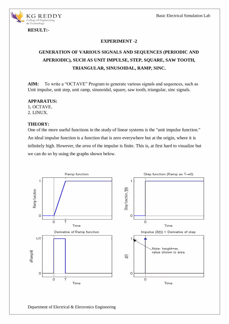
Basic Electrical Simulation Lab
Department of Electrical amp Electronics Engineering
RESULT-
EXPERIMENT -2
GENERATION OF VARIOUS SIGNALS AND SEQUENCES (PERIODIC AND
APERIODIC) SUCH AS UNIT IMPULSE STEP SQUARE SAW TOOTH
TRIANGULAR SINUSOIDAL RAMP SINC
AIM To write a ldquoOCTAVErdquo Program to generate various signals and sequences such as
Unit impulse unit step unit ramp sinusoidal square saw tooth triangular sinc signals
APPARATUS
1 OCTAVE
2 LINUX
THEORY
One of the more useful functions in the study of linear systems is the unit impulse function
An ideal impulse function is a function that is zero everywhere but at the origin where it is
infinitely high However the area of the impulse is finite This is at first hard to visualize but
we can do so by using the graphs shown below
Basic Electrical Simulation Lab
Department of Electrical amp Electronics Engineering
Unit Step Function
The unit step function and the impulse function are considered to be fundamental functions in
Engineering and it is strongly recommended that the reader becomes very familiar with both of
these functions
The unit step function also known as the Heaviside function is defined as such
Sometimes u(0) is given other values usually either 0 or 1 For many applications it is irrelevant
what the value at zero is u(0) is generally written as undefined
Sinc Function
There is a particular form that appears so frequently in communications engineering that we give
it its own name This function is called the Sinc function The Sinc function is defined in the
following manner
And Sinc(0)=1
The value of sinc(x) is defined as 1 at x = 0 since
Then since cos(0) = 1 we can apply the Squeeze Theorem to show that the sinc function
approaches one as x goes to zero Thus defining sinc(0) to be 1 makes the sinc function
continuous Also the Sinc function approaches zero as x goes towards infinity with the envelope
of sinc(x) tapering off as 1x
Basic Electrical Simulation Lab
Department of Electrical amp Electronics Engineering
Rect Function
The Rect Function is a function which produces a rectangular shaped pulse with a width of 1
centred at t = 0 The Rect function pulse also has a height of 1 The Sinc function and the
rectangular function form a Fourier transform pair
A Rect function can be written in the form
where the pulse is centered at X and has width Y We can define the impulse function above in
terms of the rectangle function by centering the pulse at zero (X = 0) setting its height to 1A and
setting the pulse width to A which approaches zero
We can also construct a Rect function out of a pair of unit step functions
Here both unit step functions are set a distance of Y2 away from the center point of (t - X)
SAW TOOTH-
The sawtooth wave (or saw wave) is a kind of non-sinusoidal waveform It is named a sawtooth
based on its resemblance to the teeth on the blade of a saw The convention is that a sawtooth
wave ramps upward and then sharply drops However there are also sawtooth waves in which the
wave ramps downward and then sharply rises The latter type of sawtooth wave is called a reverse
sawtooth wave or inverse sawtooth wave As audio signals the two orientations of sawtooth
wave sound identical The piecewise linear function based on the floor function of time t is an
example of a sawtooth wave with period 1
TRIANGLE WAVE
A triangle wave is a non-sinusoidal waveform named for its triangular shape A band
limited triangle wave pictured in the time domain (top) and frequency domain (bottom) The
fundamental is at 220 Hz (A2)Like a square wave the triangle wave contains only odd
harmonics However the higher harmonics roll off much faster than in a square wave
(proportional to the inverse square of the harmonic number as opposed to just the inverse)It is
possible to approximate a triangle wave with additive synthesis by adding odd harmonics of the
fundamental multiplying every (4n-1)th harmonic by -1and rolling off the harmonics by
the inverse square of their relative frequency to the undamental This infinite Fourier series
converges to the triangle
Basic Electrical Simulation Lab
Department of Electrical amp Electronics Engineering
SINUSOIDAL SIGNAL GENERATION
The sine wave or sinusoid is a mathematical function that describes a smooth repetitive
oscillation It occurs often in pure mathematics as well as physics signal processing electrical
engineering and many other fields Its most basic form as a function of time (t) is
where
bull A the amplitude is the peak deviation of the function from its center position
bull the angular frequency specifies how many oscillations occur in a unit time interval in
radians per second
bull the phase specifies where in its cycle the oscillation begins at t = 0
PROGRAM-
impulse
clc
clear all
close all
t=-10110
x=(t==0)
subplot(211)
plot(txb)
xlabel(time)
ylabel(amplitude)
title(unit impulse function)
subplot(212)
stem(txr)
xlabel(time)
ylabel(amplitude)
title(unit impulse discrete function)
Basic Electrical Simulation Lab
Department of Electrical amp Electronics Engineering
Step
clc
clear all
close all
N=100
t=1100
x=ones(1N)
subplot(211)
plot(txr)
xlabel(time)
ylabel(amplitude)
title(unit step function)
subplot(212)
stem(txr)
xlabel(time)
ylabel(amplitude)
title(unit step discrete function)
Ramp
clc
clear all
close all
t=020
x=t
subplot(211)
plot(txr)
xlabel(time)
ylabel(amplitude)
title(unit ramp function)
subplot(212)
stem(txr)
xlabel(time)
ylabel(amplitude)
title(unit ramp discrete function)
Basic Electrical Simulation Lab
Department of Electrical amp Electronics Engineering
Sinusoidal
clc
clear all
close all
t=0000012
x=sin(2pit)
subplot(211)
plot(txr)
xlabel(time)
ylabel(amplitude)
title(sinusoidal signal)
subplot(212)
stem(txr)
xlabel(time)
ylabel(amplitude)
title(sinusoidal sequence)
Square
clc
clear all
close all
t=00012
x=square(2pit)
subplot(211)
plot(txr)
xlabel(time)
ylabel(amplitude)
title(square signal)
subplot(212)
stem(txr)
xlabel(time)
ylabel(amplitude)
title(square sequence)
Basic Electrical Simulation Lab
Department of Electrical amp Electronics Engineering
Sawtooth
clc
clear all
close all
t=00012
x=sawtooth(2pi5t)
subplot(211)
plot(txk)
xlabel(time)
ylabel(amplitude)
title(sawtooth signal)
subplot(212)
stem(txr)
xlabel(time)
ylabel(amplitude)
title(sawtooth sequence)
Traingular
clc
clear all
close all
t=00012
x=sawtooth(2pi5t05)
subplot(211)
plot(txk)
xlabel(time)
ylabel(amplitude)
title(triangular signal)
subplot(212)
stem(txr)
xlabel(time)
ylabel(amplitude)
title(triangular sequence)
Basic Electrical Simulation Lab
Department of Electrical amp Electronics Engineering
Sinc
clc
clear all
close all
t=linspace(-55)
x=sinc(t)
subplot(211)
plot(txk)
xlabel(time)
ylabel(amplitude)
title(sinc signal)
subplot(212)
stem(txr)
xlabel(time)
ylabel(amplitude)
title(sinc sequence)
PROCEDURE-
1 Open OCTAVE
2 Open new script
3 Type the program
4 Save in current directory
5 Compile and Run the program
6 For the output see command window Figure window
OUTPUT-
RESULT-
Basic Electrical Simulation Lab
Department of Electrical amp Electronics Engineering
EXPERIMENT-3
OPERATIONS ON SIGNALS AND SEQUENCES SUCH AS ADDITION
MULTIPLICATION SCALING SHIFTING FOLDING COMPUTATION OF ENERGY
AND AVERAGE POWER
AIM To performs operations on signals and sequences such as addition multiplication
scaling shifting folding computation of energy and average power
APPARATUS
1 OCTAVE
2 LINUX
THEORY
Basic Operation on Signals
Time shifting y(t)=x(t-T)The effect that a time shift has on the appearance of a signal If T is a
positive number the time shifted signal x (t -T ) gets shifted to the right otherwise it gets shifted
left
Signal Shifting and Delay
Shifting y(n)=x(n-k) m=n-k y=x
Time reversal Y(t)=y(-t) Time reversal _ips the signal about t = 0 as seen in Figure
Signal Addition and Substraction
Addition any two signals can be added to form a third signal z (t) = x (t) + y (t)
Signal AmplificationAttuation
Basic Electrical Simulation Lab
Department of Electrical amp Electronics Engineering
MultiplicationDivition
Multiplication of two signals their product is also a signal z (t) = x (t) y (t)
folding
y(n)=x(-n) y=fliplr(x) n=-fliplr(n)
PROGRAM-
Addition and multiplication of two signals
clc
clear all
close all
t=000012
s1=6sin(2pi5t)
subplot(411)
plot(ts1g)
xlabel(time)
ylabel(amplitude)
title(first signal)
s2=8sin(2pi5t)
subplot(412)
plot(ts2r)
xlabel(time)
ylabel(amplitude)
title(second signal)
s3=s1+s2
subplot(413)
plot(ts3g)
xlabel(time)
ylabel(amplitude)
title(sum of two signals)
s4=s1s2
subplot(414)
plot(ts4g)
xlabel(time)
ylabel(amplitude)
title(multiplication of two signals)
Basic Electrical Simulation Lab
Department of Electrical amp Electronics Engineering
Amplitude scaling for signals
clc
clear all
close all
t=000012
s1=6sin(2pi5t)
subplot(311)
plot(ts1g)
xlabel(time)
ylabel(amplitude)
title(sinusoidal signal)
s2=3s1
subplot(312)
plot(ts2r)
xlabel(time)
ylabel(amplitude)
title(amplified signal)
s3=s13
subplot(313)
plot(ts3g)
xlabel(time)
ylabel(amplitude)
title(attenuated signal)
Time scaling for signals
clc
clear all
close all
t=000012
s1=6sin(2pi5t)
subplot(311)
plot(ts1g)
xlabel(time)
ylabel(amplitude)
title(sinusoidal signal)
t1=3t
subplot(312)
plot(t1s1r)
xlabel(time)
ylabel(amplitude)
title(compressed signal)
t2=t3
subplot(313)
plot(t2s1g)
xlabel(time)
ylabel(amplitude)
title(enlarged signal)
Basic Electrical Simulation Lab
Department of Electrical amp Electronics Engineering
Time shifting of a signal
clc
clear all
close all
t=000013
s1=6sin(2pi5t)
subplot(311)
plot(ts1g)
xlabel(time)
ylabel(amplitude)
title(sinusoidal signal)
t1=t+10
subplot(312)
plot(t1s1r)
xlabel(time)
ylabel(amplitude)
title(right shift of the signal)
t2=t-10
subplot(313)
plot(t2s1g)
xlabel(time)
ylabel(amplitude)
title(left shift of the signal)
Time folding of a signal
clc
clear all
close all
t=000012
s=sin(2pi5t)
m=length(s)
n=[-mm]
y=[0zeros(1m)s]
subplot(211)
plot(nyg)
xlabel(time)
ylabel(amplitude)
title(original signal)
y1=[fliplr(s)0zeros(1m)]
subplot(212)
plot(ny1r)
xlabel(time)
ylabel(amplitude)
title(folded signal)
Basic Electrical Simulation Lab
Department of Electrical amp Electronics Engineering
PROCEDURE-
1 Open OCTAVE
2 Open new script
3 Type the program
4 Save in current directory
5 Compile and Run the program
6 For the output see command window Figure window
OUTPUT-
RESULT-
Basic Electrical Simulation Lab
Department of Electrical amp Electronics Engineering
EXPERIMENT-4
MESH AND NODAL ANALYSIS OF ELECTRICAL CIRCUITS
AIM To Simulate the DC Circuit for determining the all node voltages and mesh currents using
NGPSPICE
APPARATUS
1 NGSPICE
2 LINUX
THEORY
NODAL ANALYSIS
In electric circuits analysis nodal analysis node-voltage analysis or the branch current
method is a method of determining the voltage (potential difference) between nodes (points
where elements or branches connect) in an electrical circuit in terms of the branch currents In
analyzing a circuit using Kirchhoffs circuit laws one can either do nodal analysis using
Kirchhoffs current law (KCL) or mesh analysis using Kirchhoffs voltage law (KVL) Nodal
analysis writes an equation at each electrical node requiring that the branch currents incident at a
node must sum to zero The branch currents are written in terms of the circuit node voltages As a
consequence each branch constitutive relation must give current as a function of voltage
an admittance representation For instance for a resistor Ibranch = Vbranch G where G (=1R) is
the admittance (conductance) of the resistor
Nodal analysis is possible when all the circuit elements branch constitutive relations have
an admittance representation Nodal analysis produces a compact set of equations for the network
which can be solved by hand if small or can be quickly solved using linear algebra by computer
Because of the compact system of equations many circuit simulation programs (eg SPICE) use
nodal analysis as a basis When elements do not have admittance representations a more general
extension of nodal analysis modified nodal analysis can be used
MESH ANALYSIS
Mesh analysis works by arbitrarily assigning mesh currents in the essential meshes (also referred
to as independent meshes) An essential mesh is a loop in the circuit that does not contain any
other loop Figure 1 labels the essential meshes with one two and three A mesh current is a
current that loops around the essential mesh and the equations are set solved in terms of them A
Basic Electrical Simulation Lab
Department of Electrical amp Electronics Engineering
mesh current may not correspond to any physically flowing current but the physical currents are
easily found from them It is usual practice to have all the mesh currents loop in the same
direction This helps prevent errors when writing out the equations The convention is to have all
the mesh currents looping in a clockwise direction
Solving for mesh currents instead of directly applying Kirchhoffs current law and Kirchhoffs
voltage law can greatly reduce the amount of calculation required This is because there are fewer
mesh currents than there are physical branch currents
CIRCUIT DIAGRAM
PROGRAM
Vs 1 0 DC 20V
Ra 1 2 5k
Rb 2 0 4k
Rc 3 0 1k
Is 3 2 DC 20mA
DC
end
OUTPUT-
RESULT-
Basic Electrical Simulation Lab
Department of Electrical amp Electronics Engineering
EXPERIMENT-5
APPLICATION OF NETWORK THEOREMS TO ELECTRICAL NETWORKS
AIM To Simulate the different network theorems to electrical networks using NGPSPICE
APPARATUS
1 NGSPICE
2 LINUX
THEORY
THEVENINrsquoS THEOREM
The Theveninrsquos Theorem states that ldquoAny two terminals linear bilateral DC network can
be replaced by an equivalent circuit consisting of a voltage source Vth in series with all equivalent
resistance Rthrdquo
(OR)
Thevenins theorem states that ldquoin any two terminal linear bilateral network having a
number of voltage current sources and resistances can be replaced by a simple equivalent circuit
consisting of a single voltage source in series with a resistance where the value of the voltage
source is equal to the open circuit voltage across the two terminals of the network and the
resistance is the equivalent resistance measured between the terminals with all energy sources
replaced by their internal resistancesrdquo
NORTONrsquoS THEOREM
Nortons theorem States that ldquoin any two terminal linear bilateral network with current
sources voltage sources and resistances can be replaced by an equivalent circuit consisting of a
current source in parallel with a resistance The value of the current source is the short circuit
current between the two terminals of the network and the resistance is the equivalent resistance
measured between the terminals of the network with all the energy sources replaced by their
internal resistancesrdquo
SUPERPOSITION THEOREM
This theorem states that ldquoThe response (voltage or current) in any branch of a bilateral
linear circuit having more than one independent source equals the algebraic sum of the responses
caused by each independent source acting alone where all the other independent sources are
replaced by their internal resistancerdquo
Basic Electrical Simulation Lab
Department of Electrical amp Electronics Engineering
i1 2kΩ
+
5000
+
minus minus
+
100i1 20kΩ
minus
1 3
2
A given response in a network regulating from a number of independent sources(including
initial condition source) may be computed by summing the response to each individual source
with all other sources made in operative( reduced to zero voltage or zero current)
This statement describes the property homogeneity in linear networks So it is the
combined properties off additivity and homogeneity off linear network It is a result of the linear
relation between current and volt in circuits having linear impedances
MAX POWER TRANSFER THEOREM
Max power will be delivered by network to the load if the impedance of network is
Complex conjugate of load impedance and vice versa
(or)
The maximum transformer states that ldquoA load will received maximum power from a
linear bilateral network when its load resistance is exactly equal to the Theveninrsquos resistance
of network measured looking back into the terminals of network
PROGRAM
THEVENINS THEORM
2mV -
Find Thevenin equivalent circuit
V10 1 0 2M V
R12 1 1A 2K
V1A 1A 2 DC 0V
E20 2 0 3 0 2E-4
F30 3 0 V1A 100
R30 3 0 20K
RL 3 0 1G
TF v(3) v10
END
NODE VOLTAGE NODE VOLTAGE NODE VOLTAGE NODE VOLTAGE
Basic Electrical Simulation Lab
Department of Electrical amp Electronics Engineering
NORTONS THEORM
PROGRAM
Vs 1 0 DC 20V
R1 1 2 18k
Rb 2 0 22k
Rc 2 3 33k
Is 3 0 RL
DC
end
MAXIMUM POWER TRANSFER THEOREM
PROGRAM
VS 1 0 DC 100
R1 1 2 10
R2 2 0 30
R3 1 3 20
R4 3 0 40
RL 2 3 RLOAD 1
MODEL RLOAD RES(R=25)
DC RES RLOAD(R) 0001 40 001
TF V(23) VS
PROBE
END
Basic Electrical Simulation Lab
Department of Electrical amp Electronics Engineering
SUPERPOSITION THEOREM
Program FOR CIRCUIT 1 FOR CIRCUIT 2
VDC 1 2 DC 10V VDC 1 2 DC 10V VDC 1 2 DC 0V
R1 1 3 100 R1 1 3 100 R1 1 3 100
R2 3 4 200 R2 3 4 200 R2 3 4 200
R3 3 6 470 R3 3 6 470 R3 3 6 470
R4 2 0 560 R4 2 0 560 R4 2 0 560
R5 4 5 100 R5 4 0 100 R5 4 5 100
VX 5 0 DC 10V VY 6 0 DC 0V VY 6 0 DC 0V
VY 6 0 DC 0V OP OP
OP END END
END
OUTPUT-
RESULT-
Basic Electrical Simulation Lab
Department of Electrical amp Electronics Engineering
EXPERIMET-6
WAVEFORM SYNTHESIS USING LAPLACE TRANSFORM
AIM To perform waveform synthesis using Laplace Transforms of a given signal
APPARATUS
1 OCTAVE
2 LINUX
THEORY
Bilateral Laplace transform
When one says the Laplace transform without qualification the unilateral or one-sided
transform is normally intended The Laplace transform can be alternatively defined as the bilateral
Laplace transform or two-sided Laplace transform by extending the limits of integration to be the
entire real axis If that is done the common unilateral transform simply becomes a special case of
the bilateral transform where the definition of the function being transformed is multiplied by the
Heaviside step function The bilateral Laplace transform is defined as follows
Inverse Laplace transform
The inverse Laplace transform is given by the following complex integral which is known by
various names (the Bromwich integral the Fourier-Mellin integral and Mellins inverse formula)
Example
Let y(t)=exp(t)
We have
The integral converges if sgt1 The functions exp(t) and 1(s-1) are partner functions
Basic Electrical Simulation Lab
Department of Electrical amp Electronics Engineering
PROGRAM-
Laplace Transform
clc
clear all
close all
syms t
x=exp(-2t)heaviside(t)
y=laplace(x)
disp(Laplace Transform of input signal)
y
z=ilaplace(y)
disp(Inverse Laplace Transform of input signal)
z
PROCEDURE-
1 Open OCTAVE
2 Open new script
3 Type the program
4 Save in current directory
5 Compile and Run the program
6 For the output see command window Figure window
OUTPUT-
RESULT-
Basic Electrical Simulation Lab
Department of Electrical amp Electronics Engineering
EXPERIMENT-7
LOCATING THE ZEROS AND POLES AND PLOTTING THE
POLE ZERO MAPS IN S-PLANE AND Z-PLANE FOR THE GIVEN
TRANSFER FUNCTION
AIM To locating the zeros and poles and plotting the pole zero maps in s-plane and z-plane
for the given transfer function
APPARATUS
1 OCTAVE
2 LINUX
THEORY
A Transfer Function is the ratio of the output of a system to the input of a system in the Laplace
domain considering its initial conditions to be zero If we have an input function of X(s) and an
output function Y(s) we define the transfer function H(s) to be
transfer function is the Laplace transform of a system‟ s impulse response
Given a continuous-time transfer function in the Laplace domain H(s) or a discrete-time one in
the Z-domain H(z) a zero is any value of s or z such that the transfer function is zero and a pole
is any value of s or z such that the transfer function is infinite
Zeros1 The value(s) for z where the numerator of the transfer function equals zero 2 The
complex frequencies that make the overall gain of the filter transfer function zero
Poles 1 The value(s) for z where the denominator of the transfer function equals zero 2 The
omplex frequencies that make the overall gain of the filter transfer function
infinite
Z-transforms
the Z-transform converts a discrete time-domain signal which is a sequence of real or complex
numbers into a complex frequency-domain representationThe Z-transform like many other
integral transforms can be defined as either a one-sided or two-sided transform
Basic Electrical Simulation Lab
Department of Electrical amp Electronics Engineering
Bilateral Z-transform
The bilateral or two-sided Z-transform of a discrete-time signal x[n] is the function X(z)
defined as
Unilateral Z-transform
Alternatively in cases where x[n] is defined only for n ge 0 the single-sided or unilateral
Z-transform is defined as
In signal processing this definition is used when the signal is causal
The roots of the equation P(z) = 0 correspond to the zeros of X(z)
The roots of the equation Q(z) = 0 correspond to the poles of X(z)
PROGRAM-
locating poles of zero on s-plane
clc
clear all
close all
num=input(enter numerator co-efficients)
den=input(enter denominator co-efficients)
h=tf(numden)
poles=roots(den)
zeros=roots(num)
sgrid
pzmap(h)
grid on
title(locating poles of zeros on s-plane)
Basic Electrical Simulation Lab
Department of Electrical amp Electronics Engineering
locating poles ampzeros on z-plane
clc
clear all
close all
num=input(enter numerator coefficient)
den=input(enter denominator coefficient)
p=roots(den)
z=roots(num)
zplane(pz)
grid
title(locating poler and zeros on s-plane)
PROCEDURE-
1 Open OCTAVE
2 Open new script
3 Type the program
4 Save in current directory
5 Compile and Run the program
6 For the output see command window Figure window
OUTPUT-
RESULT-
Basic Electrical Simulation Lab
Department of Electrical amp Electronics Engineering
EXPERIMENT-8
SIMULATION OF DC CIRCUITS
AIM To Simulate the DC network using PSPICE
APPARATUS
1 NGSPICE
2 LINUX
THEORY
Generally speaking network analysis is any structured technique used to mathematically
analyze a circuit (a ldquonetworkrdquo of interconnected components) Quite often the technician or
engineer will encounter circuits containing multiple sources of power or component
configurations which defy simplification by seriesparallel analysis techniques In those cases he
or she will be forced to use other means This chapter presents a few techniques useful in
analyzing such complex circuits
To analyse the above circuit one would first find the equivalent of R2 and R3 in parallel
then add R1 in series to arrive at a total resistance Then taking the voltage of battery B1 with
that total circuit resistance the total current could be calculated through the use of Ohmrsquos
Law (I=ER) then that current figure used to calculate voltage drops in the circuit All in all a
fairly simple procedure However the addition of just one more battery could change all of that
PROGRAM
Basic Electrical Simulation Lab
Department of Electrical amp Electronics Engineering
Vs 1 0 DC 20V
Ra 1 2 5k
Rb 2 0 4k
Rc 3 0 1k
Is 3 2 DC 20mA
DC
end
OUTPUT-
RESULT-
Basic Electrical Simulation Lab
Department of Electrical amp Electronics Engineering
EXPERIMENT-9
TRANSIENT ANALYSIS
AIM To find out the transient response by simulation of RLC circuits Using NGSPICE
APPARATUS
1 NGSPICE
2 LINUX
THEORY
The transient simulation is the calculation of a networks response on arbitrary excitations The
results are network quantities (branch currents and node voltages) as a function of time
Substantial for the transient analysis is the consideration of energy storing components ie
inductors and capacitorsThe relations between current and voltage of ideal capacitors and
inductors are given by
(61)
Or in terms of differential equations
(62)
To calculate these quantities in a computer program numerical integration methods are required
With the current-voltage relations of these components at hand it is possible to apply the modified
nodal analysis algorithm in order to calculate the networks response This means the transient
analysis attempts to find an approximation to the analytical solution at discrete time points using
numeric integration
CIRCUIT DIAGRAM
Basic Electrical Simulation Lab
Department of Electrical amp Electronics Engineering
PROGRAM
VIN1 1 0 PWL(0 0 1NS 1V 1MS 1V)
VIN2 4 0 PWL(0 0 1NS 1V 1MS 1V)
VIN3 7 0 PWL(0 0 1NS 1V 1MS 1V)
R1 1 2 2
R2 4 5 1
R3 7 8 8
L1 2 3 50UH
L2 5 6 50UH
L3 8 9 50UH
C1 3 0 10UF
C2 6 0 10UF
C3 9 0 10UF
TRAN 1US 400US
PLOT TRAN V(3) V(6) V(9)
PROBE
END
OUTPUT-
RESULT-
Basic Electrical Simulation Lab
Department of Electrical amp Electronics Engineering
EXPERIMENT-10
SIMULATION OF SINGLE PHASE DIODE BRIDGE RECTIFIERS WITH FILTER FOR
R amp RL LOAD
AIM To analyze the simulation of 1-Oslash diode bridge rectifiers with filter for R amp RL load using
NGSPICE
APPARATUS
1 NGSPICE
2 LINUX
THEORY
A bridge rectifier circuit is a common part of the electronic power supplies
Many electronic circuits require rectified DC power supply for powering the various electronic
basic components from available AC mains supply We can find this rectifier in a wide variety of
electronic AC power devices like home appliances motor controllers modulation process
welding applications etc
A Bridge rectifier is an Alternating Current (AC) to Direct Current (DC) converter that
rectifies mains AC input to DC output Bridge Rectifiers are widely used in power supplies that
provide necessary DC voltage for the electronic components or devices They can be constructed
with four or more diodes or any other controlled solid state switches Depending on the load
current requirements a proper bridge rectifier is selected Componentsrsquo ratings and specifications
breakdown voltage temperature ranges transient current rating forward current rating mounting
requirements and other considerations are taken into account while selecting a rectifier power
supply for an appropriate electronic circuitrsquos application
Bride rectifiers are classified into several types based on these factors type of supply
controlling capability bride circuitrsquos configurations etc Bridge rectifiers are mainly classified
into single and three phase rectifiers Both these types are further classified into uncontrolled half
controlled and full controlled rectifiers
Basic Electrical Simulation Lab
Department of Electrical amp Electronics Engineering
Program
VS 1 0 SIN(0 1697V 60HZ)
DF 5 4 DMOD
R1 4 7 10
L1 7 8 20MH
C1 4 6 793UF
RX 6 5 01
VX 8 5 DC 10V
VY 2 1 DC 0V
D1 2 4 DMOD
D2 5 3 DMOD
D3 3 4 DMOD
D4 5 2 DMOD
MODEL DMOD D( IS=22E-15 BV=1800 TT=0)
TRAN 10US 100MS 166MS
PROBE
FOUR 120HZ I(VX)
END
OUTPUT-
RESULT-
Basic Electrical Simulation Lab
Department of Electrical amp Electronics Engineering
EXPERIMENT-11
SIMULATION OF THREE PHASE DIODE BRIDGE RECTIFIERS WITH R RL LOAD
AIM To analyze the simulation of 3-Oslash diode bridge rectifiers with filter for R amp RL load using
NGSPICE
APPARATUS
1 NGSPICE
2 LINUX
THEORY
Three phase half controlled bridge converters amp fully controlled bridge converters are used
extensively in industrial applications up to about 15kW of output power The Three phase
controlled rectifiers provide a maximum dc output of
vdc(max)=2vm prod
The output ripple frequency is equal to the twice the ac supply frequency The single phase
full wave controlled rectifiers provide two output pulses during every input supply cycle
and hence are referred to as two pulse converters
Three phase converters are 3-phase controlled rectifiers which are used to convert ac input
power supply into dc output power across the load
Features of 3-phase controlled rectifiers are
Operate from 3 phase ac supply voltage
They provide higher dc output voltage and higher dc output power
Higher output voltage ripple frequency
Filtering requirements are simplified for smoothing out load voltage and load
current
Three phase controlled rectifiers are extensively used in high power variable speed
industrial dc drives
Basic Electrical Simulation Lab
Department of Electrical amp Electronics Engineering
Program
VAN 1 0 SIN(0V 200V 50HZ 0 0 0)
VBN 2 0 SIN(0V 200V 50HZ 0 0 -120)
VCN 3 0 SIN(0V 200V 50HZ 0 0 -240)
R 7 9 20
L 9 10 55MH
VX 10 8 DC 0V
VY 1 4 DC 0V
D1 4 7 DMOD
D2 8 2 DMOD
D3 3 7 DMOD
D4 8 4 DMOD
D5 2 7 DMOD
D6 8 3 DMOD
MODEL DMOD D(IS=22E-15 BV=1800V TT=0)
TRAN 5US 50MS 2166MS
PROBE
END
OUTPUT-
RESULT-
Basic Electrical Simulation Lab
Department of Electrical amp Electronics Engineering
EXPERIMENT-12
DESIGN OF LOW PASS AND HIGH PASS FILTERS
AIM To analyze the simulation of 3-Oslash diode bridge rectifiers with filter for R amp RL load using
NGSPICE
APPARATUS
1 OCTAVE
2 LINUX
THEORY
A filter is a circuit that has designed to pass a specified band of frequencies while attenuating all
signals outside this band Active filters employ transistors or op-amps plus resistors inductors
and capacitors There are four types of filters low-pass high-pass band-pass and band-
elimination (also referred to as band-reject or notch) filters Figure 71 illustrates frequency-
response plot for the four types of filters A low-pass filter is a circuit that has a constant output
voltage from dc up to a cutoff frequency fc As the frequency increases above fc the output
voltage is attenuated (decreases) Figure 71(a) is a plot of magnitude of the output voltage of a
low-pass filter versus frequency The range of frequencies that are transmitted is known as the
pass-band The range of frequencies that are attenuated is known as the stop-band The cutoff
frequency fc is also called the 0707 frequency the 3-dB frequency the corner frequency or the
break frequency High-pass filters attenuate the output voltage for all frequencies below the cutoff
frequency fc Above fc the magnitude of the output voltage is constant Figure 71(b) is the plot
for ideal and practical high-pass filters Band-pass filters pass only a band of frequencies while
attenuating all frequencies outside the band Band-elimination filters perform in an exactly
opposite way that is band-elimination filters reject a specified band of frequencies while passing
all frequencies outside the band Typical frequency-response plots for band-pass and band-
elimination filters are shown in Figure 71(c) and (d) In many filter applications it is necessary
for the closed-loop gain to be as close to 1 as possible within the pass band The Butterworth filter
is best suited for this type of application The Butterworth filter is also called a maximally flat or
flat-flat filter and all filter in this experiment will be of the Butterworth type Figure 72 shows
the ideal and the practical frequency response for three types of Butterworth filters As the roll-
offs become steeper they approach the ideal filter more closely
Basic Electrical Simulation Lab
Department of Electrical amp Electronics Engineering
PROGRAM
LOW PASS FILTER
N = 100 FIR filter order
Fp = 20e3 20 kHz passband-edge frequency
Fs = 96e3 96 kHz sampling frequency
Rp = 000057565 Corresponds to 001 dB peak-to-peak ripple
Rst = 1e-4 Corresponds to 80 dB stopband attenuation
eqnum = firceqrip(NFp(Fs2)[Rp Rst]passedge) eqnum = vec of coeffs
fvtool(eqnumFsFsColorWhite) Visualize filter
HIGH PASS FILTER
Fstop = 350
Fpass = 400
Astop = 65
Apass = 05
Fs = 1e3
d = designfilt(highpassfirStopbandFrequencyFstop
PassbandFrequencyFpassStopbandAttenuationAstop
PassbandRippleApassSampleRateFsDesignMethodequiripple)
fvtool(d)
OUTPUT-
RESULT-
Basic Electrical Simulation Lab
Department of Electrical amp Electronics Engineering
EXPERIMENT-13
FINDING THE EVEN AND ODD PARTS OF SIGNAL SEQUENCE AND REAL AND
IMAGINARY PARTS OF SIGNAL
AIM
program for finding even and odd parts of sequences Using OCTAVE Softwareamp
program for finding real and imaginary parts of sequences Using OCTAVE Software
APPARATUS
1 OCTAVE
2 LINUX
THEORY
Even and Odd Signal
One of characteristics of signal is symmetry that may be useful for signal analysis Even signals
are symmetric around vertical axis and Odd signals are symmetric about origin
Even Signal A signal is referred to as an even if it is identical to its time-reversed counterparts
x(t) = x(-t)
Odd Signal A signal is odd if x(t) = -x(-t)
An odd signal must be 0 at t=0 in other words odd signal passes the origin
Using the definition of even and odd signal any signal may be decomposed into a sum of its even
part xe(t) and its odd part xo(t) as follows
x(t)=xe(t)+xo(t)
x(t)=12x(t)+x(-t) +12x(t)-x(-t)
where
xe(t)=12x(t)+x(-t) ampxo(t)=12x(t)-x(-t)
It is an important fact because it is relative concept of Fourier series In Fourier series aperiodic
signal can be broken into a sum of sine and cosine signals Notice that sine function is odd signal
and cosine function is even signal
ENERGY AND POWER SIGNAL
A signal can be categorized into energy signal or power
signal An energy signal has a finite energy 0 lt E lt 1049279 In other words energy signals have
values only in the limited time duration For example a signal having only one square pulse is
energy signal A signal that decays exponentially has finite energy so it is also an energy signal
The power of an energy signal is 0 because of dividing finite energy by infinite time (or length)
If x(t) is a real-valued signal with Fourier transform X(f) and u(f) is the Heaviside step function
Basic Electrical Simulation Lab
Department of Electrical amp Electronics Engineering
then the function
contains only the non-negative frequency components of X(f) And the operation is reversible due
to the Hermitian property of X(f)
X(f) denotes the complex conjugate of X(f)
The inverse Fourier transform of Xa(f) is the analytic signal
where x^(t) is the Hilbert transform of x(t) and J is the imaginary unit
Basic Electrical Simulation Lab
Department of Electrical amp Electronics Engineering
PROGRAM-
Evenoddrealimaginary parts of a sequences
clc
clear all
close all
h=input(enter noof samples)
m=(h-1)2
n=-mm
x=input(enter sample values)
subplot(411)
stem(nxg)
xlabel(time)
ylabel(amplitude)
title(original sequence)
xmir=fliplr(x)
subplot(412)
stem(nxmirr)
xlabel(time)
ylabel(amplitude)
title(folded sequence)
even part of sequence
xeven=(x+xmir)2
subplot(413)
stem(nxevenr)
xlabel(time)
ylabel(amplitude)
title(even part of sequence)
odd part of sequence
xodd=(x-xmir)2
subplot(414)
stem(nxoddg)
xlabel(time)
ylabel(amplitude)
title(odd part of sequence)
Basic Electrical Simulation Lab
Department of Electrical amp Electronics Engineering
RealampImaginary parts of a sequences
clc
clear all
close all
y=input(enter complex numbers)
yreal=real(y)
disp(real values of y)
yreal
yimag=imag(y)
disp(imaginary values of y)
yimag
PROCEDURE-
1 Open OCTAVE
2 Open new script
3 Type the program
4 Save in current directory
5 Compile and Run the program
6 For the output see command window Figure window
OUTPUT-
RESULT-
Basic Electrical Simulation Lab
Department of Electrical amp Electronics Engineering
EXPERIMENT-14
FINDING THE FOURIER TRANSFORM OF A GIVEN SIGNAL AND PLOTTING ITS
MAGNITUDE AND PHASE SPECTRUM
AIM
Program for finding the fourier transform of a given signal Using OCTAVE Software amp Plotting
Its Magnitude And Phase Spectrum Using OCTAVE Software
APPARATUS
1 OCTAVE
2 LINUX
THEORY
The Fourier transform (FT) decomposes a function of time (a signal) into the
frequencies that make it up in a way similar to how a musical chord can be expressed as the
frequencies (or pitches) of its constituent notes The Fourier transform of a function of time itself
is a complex-valued function of frequency whose absolute value represents the amount of that
frequency present in the original function and whose complex argument is the phase offset of the
basic sinusoid in that frequency The Fourier transform is called the frequency domain
representation of the original signal The term Fourier transform refers to both the frequency
domain representation and the mathematical operation that associates the frequency domain
representation to a function of time The Fourier transform is not limited to functions of time but
in order to have a unified language the domain of the original function is commonly referred to as
the time domain For many functions of practical interest one can define an operation that
reverses this the inverse Fourier transformation also called Fourier synthesis of a frequency
domain representation combines the contributions of all the different frequencies to recover the
original function of time
Linear operations performed in one domain (time or frequency) have corresponding
operations in the other domain which are sometimes easier to perform The operation
of differentiation in the time domain corresponds to multiplication by the frequency[remark 1] so
some differential equations are easier to analyze in the frequency domain Also convolution in the
time domain corresponds to ordinary multiplication in the frequency domain Concretely this
means that any linear time-invariant system such as a filter applied to a signal can be expressed
relatively simply as an operation on frequencies After performing the desired operations
transformation of the result can be made back to the time domain Harmonic analysis is the
systematic study of the relationship between the frequency and time domains including the kinds
Basic Electrical Simulation Lab
Department of Electrical amp Electronics Engineering
of functions or operations that are simpler in one or the other and has deep connections to many
areas of modern mathematics
PROGRAM
Fs = 1000 Sampling frequency
T = 1Fs Sampling period
L = 1500 Length of signal
t = (0L-1)T Time vector
S = 07sin(2pi50t) + sin(2pi120t)
X = S + 2randn(size(t))
plot(1000t(150)X(150))
title(Signal Corrupted with Zero-Mean Random Noise)
xlabel(t (milliseconds))
ylabel(X(t))
Y = fft(X)
P2 = abs(YL)
P1 = P2(1L2+1)
P1(2end-1) = 2P1(2end-1)
f = Fs(0(L2))L
plot(fP1)
title(Single-Sided Amplitude Spectrum of X(t))
xlabel(f (Hz))
ylabel(|P1(f)|)
Y = fft(S)
P2 = abs(YL)
P1 = P2(1L2+1)
P1(2end-1) = 2P1(2end-1)
plot(fP1)
title(Single-Sided Amplitude Spectrum of S(t))
xlabel(f (Hz))
ylabel(|P1(f)|)
OUTPUT-
RESULT-
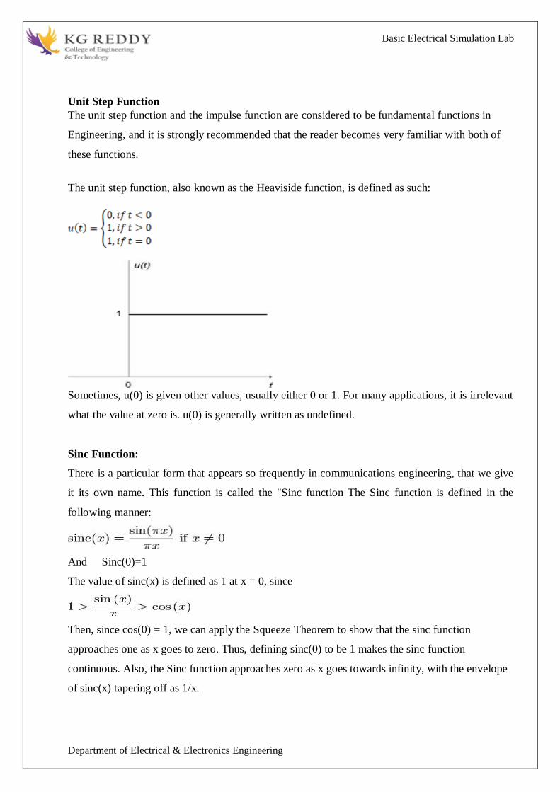
Basic Electrical Simulation Lab
Department of Electrical amp Electronics Engineering
Unit Step Function
The unit step function and the impulse function are considered to be fundamental functions in
Engineering and it is strongly recommended that the reader becomes very familiar with both of
these functions
The unit step function also known as the Heaviside function is defined as such
Sometimes u(0) is given other values usually either 0 or 1 For many applications it is irrelevant
what the value at zero is u(0) is generally written as undefined
Sinc Function
There is a particular form that appears so frequently in communications engineering that we give
it its own name This function is called the Sinc function The Sinc function is defined in the
following manner
And Sinc(0)=1
The value of sinc(x) is defined as 1 at x = 0 since
Then since cos(0) = 1 we can apply the Squeeze Theorem to show that the sinc function
approaches one as x goes to zero Thus defining sinc(0) to be 1 makes the sinc function
continuous Also the Sinc function approaches zero as x goes towards infinity with the envelope
of sinc(x) tapering off as 1x
Basic Electrical Simulation Lab
Department of Electrical amp Electronics Engineering
Rect Function
The Rect Function is a function which produces a rectangular shaped pulse with a width of 1
centred at t = 0 The Rect function pulse also has a height of 1 The Sinc function and the
rectangular function form a Fourier transform pair
A Rect function can be written in the form
where the pulse is centered at X and has width Y We can define the impulse function above in
terms of the rectangle function by centering the pulse at zero (X = 0) setting its height to 1A and
setting the pulse width to A which approaches zero
We can also construct a Rect function out of a pair of unit step functions
Here both unit step functions are set a distance of Y2 away from the center point of (t - X)
SAW TOOTH-
The sawtooth wave (or saw wave) is a kind of non-sinusoidal waveform It is named a sawtooth
based on its resemblance to the teeth on the blade of a saw The convention is that a sawtooth
wave ramps upward and then sharply drops However there are also sawtooth waves in which the
wave ramps downward and then sharply rises The latter type of sawtooth wave is called a reverse
sawtooth wave or inverse sawtooth wave As audio signals the two orientations of sawtooth
wave sound identical The piecewise linear function based on the floor function of time t is an
example of a sawtooth wave with period 1
TRIANGLE WAVE
A triangle wave is a non-sinusoidal waveform named for its triangular shape A band
limited triangle wave pictured in the time domain (top) and frequency domain (bottom) The
fundamental is at 220 Hz (A2)Like a square wave the triangle wave contains only odd
harmonics However the higher harmonics roll off much faster than in a square wave
(proportional to the inverse square of the harmonic number as opposed to just the inverse)It is
possible to approximate a triangle wave with additive synthesis by adding odd harmonics of the
fundamental multiplying every (4n-1)th harmonic by -1and rolling off the harmonics by
the inverse square of their relative frequency to the undamental This infinite Fourier series
converges to the triangle
Basic Electrical Simulation Lab
Department of Electrical amp Electronics Engineering
SINUSOIDAL SIGNAL GENERATION
The sine wave or sinusoid is a mathematical function that describes a smooth repetitive
oscillation It occurs often in pure mathematics as well as physics signal processing electrical
engineering and many other fields Its most basic form as a function of time (t) is
where
bull A the amplitude is the peak deviation of the function from its center position
bull the angular frequency specifies how many oscillations occur in a unit time interval in
radians per second
bull the phase specifies where in its cycle the oscillation begins at t = 0
PROGRAM-
impulse
clc
clear all
close all
t=-10110
x=(t==0)
subplot(211)
plot(txb)
xlabel(time)
ylabel(amplitude)
title(unit impulse function)
subplot(212)
stem(txr)
xlabel(time)
ylabel(amplitude)
title(unit impulse discrete function)
Basic Electrical Simulation Lab
Department of Electrical amp Electronics Engineering
Step
clc
clear all
close all
N=100
t=1100
x=ones(1N)
subplot(211)
plot(txr)
xlabel(time)
ylabel(amplitude)
title(unit step function)
subplot(212)
stem(txr)
xlabel(time)
ylabel(amplitude)
title(unit step discrete function)
Ramp
clc
clear all
close all
t=020
x=t
subplot(211)
plot(txr)
xlabel(time)
ylabel(amplitude)
title(unit ramp function)
subplot(212)
stem(txr)
xlabel(time)
ylabel(amplitude)
title(unit ramp discrete function)
Basic Electrical Simulation Lab
Department of Electrical amp Electronics Engineering
Sinusoidal
clc
clear all
close all
t=0000012
x=sin(2pit)
subplot(211)
plot(txr)
xlabel(time)
ylabel(amplitude)
title(sinusoidal signal)
subplot(212)
stem(txr)
xlabel(time)
ylabel(amplitude)
title(sinusoidal sequence)
Square
clc
clear all
close all
t=00012
x=square(2pit)
subplot(211)
plot(txr)
xlabel(time)
ylabel(amplitude)
title(square signal)
subplot(212)
stem(txr)
xlabel(time)
ylabel(amplitude)
title(square sequence)
Basic Electrical Simulation Lab
Department of Electrical amp Electronics Engineering
Sawtooth
clc
clear all
close all
t=00012
x=sawtooth(2pi5t)
subplot(211)
plot(txk)
xlabel(time)
ylabel(amplitude)
title(sawtooth signal)
subplot(212)
stem(txr)
xlabel(time)
ylabel(amplitude)
title(sawtooth sequence)
Traingular
clc
clear all
close all
t=00012
x=sawtooth(2pi5t05)
subplot(211)
plot(txk)
xlabel(time)
ylabel(amplitude)
title(triangular signal)
subplot(212)
stem(txr)
xlabel(time)
ylabel(amplitude)
title(triangular sequence)
Basic Electrical Simulation Lab
Department of Electrical amp Electronics Engineering
Sinc
clc
clear all
close all
t=linspace(-55)
x=sinc(t)
subplot(211)
plot(txk)
xlabel(time)
ylabel(amplitude)
title(sinc signal)
subplot(212)
stem(txr)
xlabel(time)
ylabel(amplitude)
title(sinc sequence)
PROCEDURE-
1 Open OCTAVE
2 Open new script
3 Type the program
4 Save in current directory
5 Compile and Run the program
6 For the output see command window Figure window
OUTPUT-
RESULT-
Basic Electrical Simulation Lab
Department of Electrical amp Electronics Engineering
EXPERIMENT-3
OPERATIONS ON SIGNALS AND SEQUENCES SUCH AS ADDITION
MULTIPLICATION SCALING SHIFTING FOLDING COMPUTATION OF ENERGY
AND AVERAGE POWER
AIM To performs operations on signals and sequences such as addition multiplication
scaling shifting folding computation of energy and average power
APPARATUS
1 OCTAVE
2 LINUX
THEORY
Basic Operation on Signals
Time shifting y(t)=x(t-T)The effect that a time shift has on the appearance of a signal If T is a
positive number the time shifted signal x (t -T ) gets shifted to the right otherwise it gets shifted
left
Signal Shifting and Delay
Shifting y(n)=x(n-k) m=n-k y=x
Time reversal Y(t)=y(-t) Time reversal _ips the signal about t = 0 as seen in Figure
Signal Addition and Substraction
Addition any two signals can be added to form a third signal z (t) = x (t) + y (t)
Signal AmplificationAttuation
Basic Electrical Simulation Lab
Department of Electrical amp Electronics Engineering
MultiplicationDivition
Multiplication of two signals their product is also a signal z (t) = x (t) y (t)
folding
y(n)=x(-n) y=fliplr(x) n=-fliplr(n)
PROGRAM-
Addition and multiplication of two signals
clc
clear all
close all
t=000012
s1=6sin(2pi5t)
subplot(411)
plot(ts1g)
xlabel(time)
ylabel(amplitude)
title(first signal)
s2=8sin(2pi5t)
subplot(412)
plot(ts2r)
xlabel(time)
ylabel(amplitude)
title(second signal)
s3=s1+s2
subplot(413)
plot(ts3g)
xlabel(time)
ylabel(amplitude)
title(sum of two signals)
s4=s1s2
subplot(414)
plot(ts4g)
xlabel(time)
ylabel(amplitude)
title(multiplication of two signals)
Basic Electrical Simulation Lab
Department of Electrical amp Electronics Engineering
Amplitude scaling for signals
clc
clear all
close all
t=000012
s1=6sin(2pi5t)
subplot(311)
plot(ts1g)
xlabel(time)
ylabel(amplitude)
title(sinusoidal signal)
s2=3s1
subplot(312)
plot(ts2r)
xlabel(time)
ylabel(amplitude)
title(amplified signal)
s3=s13
subplot(313)
plot(ts3g)
xlabel(time)
ylabel(amplitude)
title(attenuated signal)
Time scaling for signals
clc
clear all
close all
t=000012
s1=6sin(2pi5t)
subplot(311)
plot(ts1g)
xlabel(time)
ylabel(amplitude)
title(sinusoidal signal)
t1=3t
subplot(312)
plot(t1s1r)
xlabel(time)
ylabel(amplitude)
title(compressed signal)
t2=t3
subplot(313)
plot(t2s1g)
xlabel(time)
ylabel(amplitude)
title(enlarged signal)
Basic Electrical Simulation Lab
Department of Electrical amp Electronics Engineering
Time shifting of a signal
clc
clear all
close all
t=000013
s1=6sin(2pi5t)
subplot(311)
plot(ts1g)
xlabel(time)
ylabel(amplitude)
title(sinusoidal signal)
t1=t+10
subplot(312)
plot(t1s1r)
xlabel(time)
ylabel(amplitude)
title(right shift of the signal)
t2=t-10
subplot(313)
plot(t2s1g)
xlabel(time)
ylabel(amplitude)
title(left shift of the signal)
Time folding of a signal
clc
clear all
close all
t=000012
s=sin(2pi5t)
m=length(s)
n=[-mm]
y=[0zeros(1m)s]
subplot(211)
plot(nyg)
xlabel(time)
ylabel(amplitude)
title(original signal)
y1=[fliplr(s)0zeros(1m)]
subplot(212)
plot(ny1r)
xlabel(time)
ylabel(amplitude)
title(folded signal)
Basic Electrical Simulation Lab
Department of Electrical amp Electronics Engineering
PROCEDURE-
1 Open OCTAVE
2 Open new script
3 Type the program
4 Save in current directory
5 Compile and Run the program
6 For the output see command window Figure window
OUTPUT-
RESULT-
Basic Electrical Simulation Lab
Department of Electrical amp Electronics Engineering
EXPERIMENT-4
MESH AND NODAL ANALYSIS OF ELECTRICAL CIRCUITS
AIM To Simulate the DC Circuit for determining the all node voltages and mesh currents using
NGPSPICE
APPARATUS
1 NGSPICE
2 LINUX
THEORY
NODAL ANALYSIS
In electric circuits analysis nodal analysis node-voltage analysis or the branch current
method is a method of determining the voltage (potential difference) between nodes (points
where elements or branches connect) in an electrical circuit in terms of the branch currents In
analyzing a circuit using Kirchhoffs circuit laws one can either do nodal analysis using
Kirchhoffs current law (KCL) or mesh analysis using Kirchhoffs voltage law (KVL) Nodal
analysis writes an equation at each electrical node requiring that the branch currents incident at a
node must sum to zero The branch currents are written in terms of the circuit node voltages As a
consequence each branch constitutive relation must give current as a function of voltage
an admittance representation For instance for a resistor Ibranch = Vbranch G where G (=1R) is
the admittance (conductance) of the resistor
Nodal analysis is possible when all the circuit elements branch constitutive relations have
an admittance representation Nodal analysis produces a compact set of equations for the network
which can be solved by hand if small or can be quickly solved using linear algebra by computer
Because of the compact system of equations many circuit simulation programs (eg SPICE) use
nodal analysis as a basis When elements do not have admittance representations a more general
extension of nodal analysis modified nodal analysis can be used
MESH ANALYSIS
Mesh analysis works by arbitrarily assigning mesh currents in the essential meshes (also referred
to as independent meshes) An essential mesh is a loop in the circuit that does not contain any
other loop Figure 1 labels the essential meshes with one two and three A mesh current is a
current that loops around the essential mesh and the equations are set solved in terms of them A
Basic Electrical Simulation Lab
Department of Electrical amp Electronics Engineering
mesh current may not correspond to any physically flowing current but the physical currents are
easily found from them It is usual practice to have all the mesh currents loop in the same
direction This helps prevent errors when writing out the equations The convention is to have all
the mesh currents looping in a clockwise direction
Solving for mesh currents instead of directly applying Kirchhoffs current law and Kirchhoffs
voltage law can greatly reduce the amount of calculation required This is because there are fewer
mesh currents than there are physical branch currents
CIRCUIT DIAGRAM
PROGRAM
Vs 1 0 DC 20V
Ra 1 2 5k
Rb 2 0 4k
Rc 3 0 1k
Is 3 2 DC 20mA
DC
end
OUTPUT-
RESULT-
Basic Electrical Simulation Lab
Department of Electrical amp Electronics Engineering
EXPERIMENT-5
APPLICATION OF NETWORK THEOREMS TO ELECTRICAL NETWORKS
AIM To Simulate the different network theorems to electrical networks using NGPSPICE
APPARATUS
1 NGSPICE
2 LINUX
THEORY
THEVENINrsquoS THEOREM
The Theveninrsquos Theorem states that ldquoAny two terminals linear bilateral DC network can
be replaced by an equivalent circuit consisting of a voltage source Vth in series with all equivalent
resistance Rthrdquo
(OR)
Thevenins theorem states that ldquoin any two terminal linear bilateral network having a
number of voltage current sources and resistances can be replaced by a simple equivalent circuit
consisting of a single voltage source in series with a resistance where the value of the voltage
source is equal to the open circuit voltage across the two terminals of the network and the
resistance is the equivalent resistance measured between the terminals with all energy sources
replaced by their internal resistancesrdquo
NORTONrsquoS THEOREM
Nortons theorem States that ldquoin any two terminal linear bilateral network with current
sources voltage sources and resistances can be replaced by an equivalent circuit consisting of a
current source in parallel with a resistance The value of the current source is the short circuit
current between the two terminals of the network and the resistance is the equivalent resistance
measured between the terminals of the network with all the energy sources replaced by their
internal resistancesrdquo
SUPERPOSITION THEOREM
This theorem states that ldquoThe response (voltage or current) in any branch of a bilateral
linear circuit having more than one independent source equals the algebraic sum of the responses
caused by each independent source acting alone where all the other independent sources are
replaced by their internal resistancerdquo
Basic Electrical Simulation Lab
Department of Electrical amp Electronics Engineering
i1 2kΩ
+
5000
+
minus minus
+
100i1 20kΩ
minus
1 3
2
A given response in a network regulating from a number of independent sources(including
initial condition source) may be computed by summing the response to each individual source
with all other sources made in operative( reduced to zero voltage or zero current)
This statement describes the property homogeneity in linear networks So it is the
combined properties off additivity and homogeneity off linear network It is a result of the linear
relation between current and volt in circuits having linear impedances
MAX POWER TRANSFER THEOREM
Max power will be delivered by network to the load if the impedance of network is
Complex conjugate of load impedance and vice versa
(or)
The maximum transformer states that ldquoA load will received maximum power from a
linear bilateral network when its load resistance is exactly equal to the Theveninrsquos resistance
of network measured looking back into the terminals of network
PROGRAM
THEVENINS THEORM
2mV -
Find Thevenin equivalent circuit
V10 1 0 2M V
R12 1 1A 2K
V1A 1A 2 DC 0V
E20 2 0 3 0 2E-4
F30 3 0 V1A 100
R30 3 0 20K
RL 3 0 1G
TF v(3) v10
END
NODE VOLTAGE NODE VOLTAGE NODE VOLTAGE NODE VOLTAGE
Basic Electrical Simulation Lab
Department of Electrical amp Electronics Engineering
NORTONS THEORM
PROGRAM
Vs 1 0 DC 20V
R1 1 2 18k
Rb 2 0 22k
Rc 2 3 33k
Is 3 0 RL
DC
end
MAXIMUM POWER TRANSFER THEOREM
PROGRAM
VS 1 0 DC 100
R1 1 2 10
R2 2 0 30
R3 1 3 20
R4 3 0 40
RL 2 3 RLOAD 1
MODEL RLOAD RES(R=25)
DC RES RLOAD(R) 0001 40 001
TF V(23) VS
PROBE
END
Basic Electrical Simulation Lab
Department of Electrical amp Electronics Engineering
SUPERPOSITION THEOREM
Program FOR CIRCUIT 1 FOR CIRCUIT 2
VDC 1 2 DC 10V VDC 1 2 DC 10V VDC 1 2 DC 0V
R1 1 3 100 R1 1 3 100 R1 1 3 100
R2 3 4 200 R2 3 4 200 R2 3 4 200
R3 3 6 470 R3 3 6 470 R3 3 6 470
R4 2 0 560 R4 2 0 560 R4 2 0 560
R5 4 5 100 R5 4 0 100 R5 4 5 100
VX 5 0 DC 10V VY 6 0 DC 0V VY 6 0 DC 0V
VY 6 0 DC 0V OP OP
OP END END
END
OUTPUT-
RESULT-
Basic Electrical Simulation Lab
Department of Electrical amp Electronics Engineering
EXPERIMET-6
WAVEFORM SYNTHESIS USING LAPLACE TRANSFORM
AIM To perform waveform synthesis using Laplace Transforms of a given signal
APPARATUS
1 OCTAVE
2 LINUX
THEORY
Bilateral Laplace transform
When one says the Laplace transform without qualification the unilateral or one-sided
transform is normally intended The Laplace transform can be alternatively defined as the bilateral
Laplace transform or two-sided Laplace transform by extending the limits of integration to be the
entire real axis If that is done the common unilateral transform simply becomes a special case of
the bilateral transform where the definition of the function being transformed is multiplied by the
Heaviside step function The bilateral Laplace transform is defined as follows
Inverse Laplace transform
The inverse Laplace transform is given by the following complex integral which is known by
various names (the Bromwich integral the Fourier-Mellin integral and Mellins inverse formula)
Example
Let y(t)=exp(t)
We have
The integral converges if sgt1 The functions exp(t) and 1(s-1) are partner functions
Basic Electrical Simulation Lab
Department of Electrical amp Electronics Engineering
PROGRAM-
Laplace Transform
clc
clear all
close all
syms t
x=exp(-2t)heaviside(t)
y=laplace(x)
disp(Laplace Transform of input signal)
y
z=ilaplace(y)
disp(Inverse Laplace Transform of input signal)
z
PROCEDURE-
1 Open OCTAVE
2 Open new script
3 Type the program
4 Save in current directory
5 Compile and Run the program
6 For the output see command window Figure window
OUTPUT-
RESULT-
Basic Electrical Simulation Lab
Department of Electrical amp Electronics Engineering
EXPERIMENT-7
LOCATING THE ZEROS AND POLES AND PLOTTING THE
POLE ZERO MAPS IN S-PLANE AND Z-PLANE FOR THE GIVEN
TRANSFER FUNCTION
AIM To locating the zeros and poles and plotting the pole zero maps in s-plane and z-plane
for the given transfer function
APPARATUS
1 OCTAVE
2 LINUX
THEORY
A Transfer Function is the ratio of the output of a system to the input of a system in the Laplace
domain considering its initial conditions to be zero If we have an input function of X(s) and an
output function Y(s) we define the transfer function H(s) to be
transfer function is the Laplace transform of a system‟ s impulse response
Given a continuous-time transfer function in the Laplace domain H(s) or a discrete-time one in
the Z-domain H(z) a zero is any value of s or z such that the transfer function is zero and a pole
is any value of s or z such that the transfer function is infinite
Zeros1 The value(s) for z where the numerator of the transfer function equals zero 2 The
complex frequencies that make the overall gain of the filter transfer function zero
Poles 1 The value(s) for z where the denominator of the transfer function equals zero 2 The
omplex frequencies that make the overall gain of the filter transfer function
infinite
Z-transforms
the Z-transform converts a discrete time-domain signal which is a sequence of real or complex
numbers into a complex frequency-domain representationThe Z-transform like many other
integral transforms can be defined as either a one-sided or two-sided transform
Basic Electrical Simulation Lab
Department of Electrical amp Electronics Engineering
Bilateral Z-transform
The bilateral or two-sided Z-transform of a discrete-time signal x[n] is the function X(z)
defined as
Unilateral Z-transform
Alternatively in cases where x[n] is defined only for n ge 0 the single-sided or unilateral
Z-transform is defined as
In signal processing this definition is used when the signal is causal
The roots of the equation P(z) = 0 correspond to the zeros of X(z)
The roots of the equation Q(z) = 0 correspond to the poles of X(z)
PROGRAM-
locating poles of zero on s-plane
clc
clear all
close all
num=input(enter numerator co-efficients)
den=input(enter denominator co-efficients)
h=tf(numden)
poles=roots(den)
zeros=roots(num)
sgrid
pzmap(h)
grid on
title(locating poles of zeros on s-plane)
Basic Electrical Simulation Lab
Department of Electrical amp Electronics Engineering
locating poles ampzeros on z-plane
clc
clear all
close all
num=input(enter numerator coefficient)
den=input(enter denominator coefficient)
p=roots(den)
z=roots(num)
zplane(pz)
grid
title(locating poler and zeros on s-plane)
PROCEDURE-
1 Open OCTAVE
2 Open new script
3 Type the program
4 Save in current directory
5 Compile and Run the program
6 For the output see command window Figure window
OUTPUT-
RESULT-
Basic Electrical Simulation Lab
Department of Electrical amp Electronics Engineering
EXPERIMENT-8
SIMULATION OF DC CIRCUITS
AIM To Simulate the DC network using PSPICE
APPARATUS
1 NGSPICE
2 LINUX
THEORY
Generally speaking network analysis is any structured technique used to mathematically
analyze a circuit (a ldquonetworkrdquo of interconnected components) Quite often the technician or
engineer will encounter circuits containing multiple sources of power or component
configurations which defy simplification by seriesparallel analysis techniques In those cases he
or she will be forced to use other means This chapter presents a few techniques useful in
analyzing such complex circuits
To analyse the above circuit one would first find the equivalent of R2 and R3 in parallel
then add R1 in series to arrive at a total resistance Then taking the voltage of battery B1 with
that total circuit resistance the total current could be calculated through the use of Ohmrsquos
Law (I=ER) then that current figure used to calculate voltage drops in the circuit All in all a
fairly simple procedure However the addition of just one more battery could change all of that
PROGRAM
Basic Electrical Simulation Lab
Department of Electrical amp Electronics Engineering
Vs 1 0 DC 20V
Ra 1 2 5k
Rb 2 0 4k
Rc 3 0 1k
Is 3 2 DC 20mA
DC
end
OUTPUT-
RESULT-
Basic Electrical Simulation Lab
Department of Electrical amp Electronics Engineering
EXPERIMENT-9
TRANSIENT ANALYSIS
AIM To find out the transient response by simulation of RLC circuits Using NGSPICE
APPARATUS
1 NGSPICE
2 LINUX
THEORY
The transient simulation is the calculation of a networks response on arbitrary excitations The
results are network quantities (branch currents and node voltages) as a function of time
Substantial for the transient analysis is the consideration of energy storing components ie
inductors and capacitorsThe relations between current and voltage of ideal capacitors and
inductors are given by
(61)
Or in terms of differential equations
(62)
To calculate these quantities in a computer program numerical integration methods are required
With the current-voltage relations of these components at hand it is possible to apply the modified
nodal analysis algorithm in order to calculate the networks response This means the transient
analysis attempts to find an approximation to the analytical solution at discrete time points using
numeric integration
CIRCUIT DIAGRAM
Basic Electrical Simulation Lab
Department of Electrical amp Electronics Engineering
PROGRAM
VIN1 1 0 PWL(0 0 1NS 1V 1MS 1V)
VIN2 4 0 PWL(0 0 1NS 1V 1MS 1V)
VIN3 7 0 PWL(0 0 1NS 1V 1MS 1V)
R1 1 2 2
R2 4 5 1
R3 7 8 8
L1 2 3 50UH
L2 5 6 50UH
L3 8 9 50UH
C1 3 0 10UF
C2 6 0 10UF
C3 9 0 10UF
TRAN 1US 400US
PLOT TRAN V(3) V(6) V(9)
PROBE
END
OUTPUT-
RESULT-
Basic Electrical Simulation Lab
Department of Electrical amp Electronics Engineering
EXPERIMENT-10
SIMULATION OF SINGLE PHASE DIODE BRIDGE RECTIFIERS WITH FILTER FOR
R amp RL LOAD
AIM To analyze the simulation of 1-Oslash diode bridge rectifiers with filter for R amp RL load using
NGSPICE
APPARATUS
1 NGSPICE
2 LINUX
THEORY
A bridge rectifier circuit is a common part of the electronic power supplies
Many electronic circuits require rectified DC power supply for powering the various electronic
basic components from available AC mains supply We can find this rectifier in a wide variety of
electronic AC power devices like home appliances motor controllers modulation process
welding applications etc
A Bridge rectifier is an Alternating Current (AC) to Direct Current (DC) converter that
rectifies mains AC input to DC output Bridge Rectifiers are widely used in power supplies that
provide necessary DC voltage for the electronic components or devices They can be constructed
with four or more diodes or any other controlled solid state switches Depending on the load
current requirements a proper bridge rectifier is selected Componentsrsquo ratings and specifications
breakdown voltage temperature ranges transient current rating forward current rating mounting
requirements and other considerations are taken into account while selecting a rectifier power
supply for an appropriate electronic circuitrsquos application
Bride rectifiers are classified into several types based on these factors type of supply
controlling capability bride circuitrsquos configurations etc Bridge rectifiers are mainly classified
into single and three phase rectifiers Both these types are further classified into uncontrolled half
controlled and full controlled rectifiers
Basic Electrical Simulation Lab
Department of Electrical amp Electronics Engineering
Program
VS 1 0 SIN(0 1697V 60HZ)
DF 5 4 DMOD
R1 4 7 10
L1 7 8 20MH
C1 4 6 793UF
RX 6 5 01
VX 8 5 DC 10V
VY 2 1 DC 0V
D1 2 4 DMOD
D2 5 3 DMOD
D3 3 4 DMOD
D4 5 2 DMOD
MODEL DMOD D( IS=22E-15 BV=1800 TT=0)
TRAN 10US 100MS 166MS
PROBE
FOUR 120HZ I(VX)
END
OUTPUT-
RESULT-
Basic Electrical Simulation Lab
Department of Electrical amp Electronics Engineering
EXPERIMENT-11
SIMULATION OF THREE PHASE DIODE BRIDGE RECTIFIERS WITH R RL LOAD
AIM To analyze the simulation of 3-Oslash diode bridge rectifiers with filter for R amp RL load using
NGSPICE
APPARATUS
1 NGSPICE
2 LINUX
THEORY
Three phase half controlled bridge converters amp fully controlled bridge converters are used
extensively in industrial applications up to about 15kW of output power The Three phase
controlled rectifiers provide a maximum dc output of
vdc(max)=2vm prod
The output ripple frequency is equal to the twice the ac supply frequency The single phase
full wave controlled rectifiers provide two output pulses during every input supply cycle
and hence are referred to as two pulse converters
Three phase converters are 3-phase controlled rectifiers which are used to convert ac input
power supply into dc output power across the load
Features of 3-phase controlled rectifiers are
Operate from 3 phase ac supply voltage
They provide higher dc output voltage and higher dc output power
Higher output voltage ripple frequency
Filtering requirements are simplified for smoothing out load voltage and load
current
Three phase controlled rectifiers are extensively used in high power variable speed
industrial dc drives
Basic Electrical Simulation Lab
Department of Electrical amp Electronics Engineering
Program
VAN 1 0 SIN(0V 200V 50HZ 0 0 0)
VBN 2 0 SIN(0V 200V 50HZ 0 0 -120)
VCN 3 0 SIN(0V 200V 50HZ 0 0 -240)
R 7 9 20
L 9 10 55MH
VX 10 8 DC 0V
VY 1 4 DC 0V
D1 4 7 DMOD
D2 8 2 DMOD
D3 3 7 DMOD
D4 8 4 DMOD
D5 2 7 DMOD
D6 8 3 DMOD
MODEL DMOD D(IS=22E-15 BV=1800V TT=0)
TRAN 5US 50MS 2166MS
PROBE
END
OUTPUT-
RESULT-
Basic Electrical Simulation Lab
Department of Electrical amp Electronics Engineering
EXPERIMENT-12
DESIGN OF LOW PASS AND HIGH PASS FILTERS
AIM To analyze the simulation of 3-Oslash diode bridge rectifiers with filter for R amp RL load using
NGSPICE
APPARATUS
1 OCTAVE
2 LINUX
THEORY
A filter is a circuit that has designed to pass a specified band of frequencies while attenuating all
signals outside this band Active filters employ transistors or op-amps plus resistors inductors
and capacitors There are four types of filters low-pass high-pass band-pass and band-
elimination (also referred to as band-reject or notch) filters Figure 71 illustrates frequency-
response plot for the four types of filters A low-pass filter is a circuit that has a constant output
voltage from dc up to a cutoff frequency fc As the frequency increases above fc the output
voltage is attenuated (decreases) Figure 71(a) is a plot of magnitude of the output voltage of a
low-pass filter versus frequency The range of frequencies that are transmitted is known as the
pass-band The range of frequencies that are attenuated is known as the stop-band The cutoff
frequency fc is also called the 0707 frequency the 3-dB frequency the corner frequency or the
break frequency High-pass filters attenuate the output voltage for all frequencies below the cutoff
frequency fc Above fc the magnitude of the output voltage is constant Figure 71(b) is the plot
for ideal and practical high-pass filters Band-pass filters pass only a band of frequencies while
attenuating all frequencies outside the band Band-elimination filters perform in an exactly
opposite way that is band-elimination filters reject a specified band of frequencies while passing
all frequencies outside the band Typical frequency-response plots for band-pass and band-
elimination filters are shown in Figure 71(c) and (d) In many filter applications it is necessary
for the closed-loop gain to be as close to 1 as possible within the pass band The Butterworth filter
is best suited for this type of application The Butterworth filter is also called a maximally flat or
flat-flat filter and all filter in this experiment will be of the Butterworth type Figure 72 shows
the ideal and the practical frequency response for three types of Butterworth filters As the roll-
offs become steeper they approach the ideal filter more closely
Basic Electrical Simulation Lab
Department of Electrical amp Electronics Engineering
PROGRAM
LOW PASS FILTER
N = 100 FIR filter order
Fp = 20e3 20 kHz passband-edge frequency
Fs = 96e3 96 kHz sampling frequency
Rp = 000057565 Corresponds to 001 dB peak-to-peak ripple
Rst = 1e-4 Corresponds to 80 dB stopband attenuation
eqnum = firceqrip(NFp(Fs2)[Rp Rst]passedge) eqnum = vec of coeffs
fvtool(eqnumFsFsColorWhite) Visualize filter
HIGH PASS FILTER
Fstop = 350
Fpass = 400
Astop = 65
Apass = 05
Fs = 1e3
d = designfilt(highpassfirStopbandFrequencyFstop
PassbandFrequencyFpassStopbandAttenuationAstop
PassbandRippleApassSampleRateFsDesignMethodequiripple)
fvtool(d)
OUTPUT-
RESULT-
Basic Electrical Simulation Lab
Department of Electrical amp Electronics Engineering
EXPERIMENT-13
FINDING THE EVEN AND ODD PARTS OF SIGNAL SEQUENCE AND REAL AND
IMAGINARY PARTS OF SIGNAL
AIM
program for finding even and odd parts of sequences Using OCTAVE Softwareamp
program for finding real and imaginary parts of sequences Using OCTAVE Software
APPARATUS
1 OCTAVE
2 LINUX
THEORY
Even and Odd Signal
One of characteristics of signal is symmetry that may be useful for signal analysis Even signals
are symmetric around vertical axis and Odd signals are symmetric about origin
Even Signal A signal is referred to as an even if it is identical to its time-reversed counterparts
x(t) = x(-t)
Odd Signal A signal is odd if x(t) = -x(-t)
An odd signal must be 0 at t=0 in other words odd signal passes the origin
Using the definition of even and odd signal any signal may be decomposed into a sum of its even
part xe(t) and its odd part xo(t) as follows
x(t)=xe(t)+xo(t)
x(t)=12x(t)+x(-t) +12x(t)-x(-t)
where
xe(t)=12x(t)+x(-t) ampxo(t)=12x(t)-x(-t)
It is an important fact because it is relative concept of Fourier series In Fourier series aperiodic
signal can be broken into a sum of sine and cosine signals Notice that sine function is odd signal
and cosine function is even signal
ENERGY AND POWER SIGNAL
A signal can be categorized into energy signal or power
signal An energy signal has a finite energy 0 lt E lt 1049279 In other words energy signals have
values only in the limited time duration For example a signal having only one square pulse is
energy signal A signal that decays exponentially has finite energy so it is also an energy signal
The power of an energy signal is 0 because of dividing finite energy by infinite time (or length)
If x(t) is a real-valued signal with Fourier transform X(f) and u(f) is the Heaviside step function
Basic Electrical Simulation Lab
Department of Electrical amp Electronics Engineering
then the function
contains only the non-negative frequency components of X(f) And the operation is reversible due
to the Hermitian property of X(f)
X(f) denotes the complex conjugate of X(f)
The inverse Fourier transform of Xa(f) is the analytic signal
where x^(t) is the Hilbert transform of x(t) and J is the imaginary unit
Basic Electrical Simulation Lab
Department of Electrical amp Electronics Engineering
PROGRAM-
Evenoddrealimaginary parts of a sequences
clc
clear all
close all
h=input(enter noof samples)
m=(h-1)2
n=-mm
x=input(enter sample values)
subplot(411)
stem(nxg)
xlabel(time)
ylabel(amplitude)
title(original sequence)
xmir=fliplr(x)
subplot(412)
stem(nxmirr)
xlabel(time)
ylabel(amplitude)
title(folded sequence)
even part of sequence
xeven=(x+xmir)2
subplot(413)
stem(nxevenr)
xlabel(time)
ylabel(amplitude)
title(even part of sequence)
odd part of sequence
xodd=(x-xmir)2
subplot(414)
stem(nxoddg)
xlabel(time)
ylabel(amplitude)
title(odd part of sequence)
Basic Electrical Simulation Lab
Department of Electrical amp Electronics Engineering
RealampImaginary parts of a sequences
clc
clear all
close all
y=input(enter complex numbers)
yreal=real(y)
disp(real values of y)
yreal
yimag=imag(y)
disp(imaginary values of y)
yimag
PROCEDURE-
1 Open OCTAVE
2 Open new script
3 Type the program
4 Save in current directory
5 Compile and Run the program
6 For the output see command window Figure window
OUTPUT-
RESULT-
Basic Electrical Simulation Lab
Department of Electrical amp Electronics Engineering
EXPERIMENT-14
FINDING THE FOURIER TRANSFORM OF A GIVEN SIGNAL AND PLOTTING ITS
MAGNITUDE AND PHASE SPECTRUM
AIM
Program for finding the fourier transform of a given signal Using OCTAVE Software amp Plotting
Its Magnitude And Phase Spectrum Using OCTAVE Software
APPARATUS
1 OCTAVE
2 LINUX
THEORY
The Fourier transform (FT) decomposes a function of time (a signal) into the
frequencies that make it up in a way similar to how a musical chord can be expressed as the
frequencies (or pitches) of its constituent notes The Fourier transform of a function of time itself
is a complex-valued function of frequency whose absolute value represents the amount of that
frequency present in the original function and whose complex argument is the phase offset of the
basic sinusoid in that frequency The Fourier transform is called the frequency domain
representation of the original signal The term Fourier transform refers to both the frequency
domain representation and the mathematical operation that associates the frequency domain
representation to a function of time The Fourier transform is not limited to functions of time but
in order to have a unified language the domain of the original function is commonly referred to as
the time domain For many functions of practical interest one can define an operation that
reverses this the inverse Fourier transformation also called Fourier synthesis of a frequency
domain representation combines the contributions of all the different frequencies to recover the
original function of time
Linear operations performed in one domain (time or frequency) have corresponding
operations in the other domain which are sometimes easier to perform The operation
of differentiation in the time domain corresponds to multiplication by the frequency[remark 1] so
some differential equations are easier to analyze in the frequency domain Also convolution in the
time domain corresponds to ordinary multiplication in the frequency domain Concretely this
means that any linear time-invariant system such as a filter applied to a signal can be expressed
relatively simply as an operation on frequencies After performing the desired operations
transformation of the result can be made back to the time domain Harmonic analysis is the
systematic study of the relationship between the frequency and time domains including the kinds
Basic Electrical Simulation Lab
Department of Electrical amp Electronics Engineering
of functions or operations that are simpler in one or the other and has deep connections to many
areas of modern mathematics
PROGRAM
Fs = 1000 Sampling frequency
T = 1Fs Sampling period
L = 1500 Length of signal
t = (0L-1)T Time vector
S = 07sin(2pi50t) + sin(2pi120t)
X = S + 2randn(size(t))
plot(1000t(150)X(150))
title(Signal Corrupted with Zero-Mean Random Noise)
xlabel(t (milliseconds))
ylabel(X(t))
Y = fft(X)
P2 = abs(YL)
P1 = P2(1L2+1)
P1(2end-1) = 2P1(2end-1)
f = Fs(0(L2))L
plot(fP1)
title(Single-Sided Amplitude Spectrum of X(t))
xlabel(f (Hz))
ylabel(|P1(f)|)
Y = fft(S)
P2 = abs(YL)
P1 = P2(1L2+1)
P1(2end-1) = 2P1(2end-1)
plot(fP1)
title(Single-Sided Amplitude Spectrum of S(t))
xlabel(f (Hz))
ylabel(|P1(f)|)
OUTPUT-
RESULT-
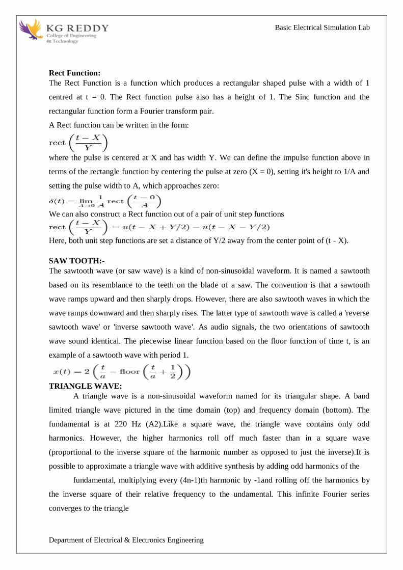
Basic Electrical Simulation Lab
Department of Electrical amp Electronics Engineering
Rect Function
The Rect Function is a function which produces a rectangular shaped pulse with a width of 1
centred at t = 0 The Rect function pulse also has a height of 1 The Sinc function and the
rectangular function form a Fourier transform pair
A Rect function can be written in the form
where the pulse is centered at X and has width Y We can define the impulse function above in
terms of the rectangle function by centering the pulse at zero (X = 0) setting its height to 1A and
setting the pulse width to A which approaches zero
We can also construct a Rect function out of a pair of unit step functions
Here both unit step functions are set a distance of Y2 away from the center point of (t - X)
SAW TOOTH-
The sawtooth wave (or saw wave) is a kind of non-sinusoidal waveform It is named a sawtooth
based on its resemblance to the teeth on the blade of a saw The convention is that a sawtooth
wave ramps upward and then sharply drops However there are also sawtooth waves in which the
wave ramps downward and then sharply rises The latter type of sawtooth wave is called a reverse
sawtooth wave or inverse sawtooth wave As audio signals the two orientations of sawtooth
wave sound identical The piecewise linear function based on the floor function of time t is an
example of a sawtooth wave with period 1
TRIANGLE WAVE
A triangle wave is a non-sinusoidal waveform named for its triangular shape A band
limited triangle wave pictured in the time domain (top) and frequency domain (bottom) The
fundamental is at 220 Hz (A2)Like a square wave the triangle wave contains only odd
harmonics However the higher harmonics roll off much faster than in a square wave
(proportional to the inverse square of the harmonic number as opposed to just the inverse)It is
possible to approximate a triangle wave with additive synthesis by adding odd harmonics of the
fundamental multiplying every (4n-1)th harmonic by -1and rolling off the harmonics by
the inverse square of their relative frequency to the undamental This infinite Fourier series
converges to the triangle
Basic Electrical Simulation Lab
Department of Electrical amp Electronics Engineering
SINUSOIDAL SIGNAL GENERATION
The sine wave or sinusoid is a mathematical function that describes a smooth repetitive
oscillation It occurs often in pure mathematics as well as physics signal processing electrical
engineering and many other fields Its most basic form as a function of time (t) is
where
bull A the amplitude is the peak deviation of the function from its center position
bull the angular frequency specifies how many oscillations occur in a unit time interval in
radians per second
bull the phase specifies where in its cycle the oscillation begins at t = 0
PROGRAM-
impulse
clc
clear all
close all
t=-10110
x=(t==0)
subplot(211)
plot(txb)
xlabel(time)
ylabel(amplitude)
title(unit impulse function)
subplot(212)
stem(txr)
xlabel(time)
ylabel(amplitude)
title(unit impulse discrete function)
Basic Electrical Simulation Lab
Department of Electrical amp Electronics Engineering
Step
clc
clear all
close all
N=100
t=1100
x=ones(1N)
subplot(211)
plot(txr)
xlabel(time)
ylabel(amplitude)
title(unit step function)
subplot(212)
stem(txr)
xlabel(time)
ylabel(amplitude)
title(unit step discrete function)
Ramp
clc
clear all
close all
t=020
x=t
subplot(211)
plot(txr)
xlabel(time)
ylabel(amplitude)
title(unit ramp function)
subplot(212)
stem(txr)
xlabel(time)
ylabel(amplitude)
title(unit ramp discrete function)
Basic Electrical Simulation Lab
Department of Electrical amp Electronics Engineering
Sinusoidal
clc
clear all
close all
t=0000012
x=sin(2pit)
subplot(211)
plot(txr)
xlabel(time)
ylabel(amplitude)
title(sinusoidal signal)
subplot(212)
stem(txr)
xlabel(time)
ylabel(amplitude)
title(sinusoidal sequence)
Square
clc
clear all
close all
t=00012
x=square(2pit)
subplot(211)
plot(txr)
xlabel(time)
ylabel(amplitude)
title(square signal)
subplot(212)
stem(txr)
xlabel(time)
ylabel(amplitude)
title(square sequence)
Basic Electrical Simulation Lab
Department of Electrical amp Electronics Engineering
Sawtooth
clc
clear all
close all
t=00012
x=sawtooth(2pi5t)
subplot(211)
plot(txk)
xlabel(time)
ylabel(amplitude)
title(sawtooth signal)
subplot(212)
stem(txr)
xlabel(time)
ylabel(amplitude)
title(sawtooth sequence)
Traingular
clc
clear all
close all
t=00012
x=sawtooth(2pi5t05)
subplot(211)
plot(txk)
xlabel(time)
ylabel(amplitude)
title(triangular signal)
subplot(212)
stem(txr)
xlabel(time)
ylabel(amplitude)
title(triangular sequence)
Basic Electrical Simulation Lab
Department of Electrical amp Electronics Engineering
Sinc
clc
clear all
close all
t=linspace(-55)
x=sinc(t)
subplot(211)
plot(txk)
xlabel(time)
ylabel(amplitude)
title(sinc signal)
subplot(212)
stem(txr)
xlabel(time)
ylabel(amplitude)
title(sinc sequence)
PROCEDURE-
1 Open OCTAVE
2 Open new script
3 Type the program
4 Save in current directory
5 Compile and Run the program
6 For the output see command window Figure window
OUTPUT-
RESULT-
Basic Electrical Simulation Lab
Department of Electrical amp Electronics Engineering
EXPERIMENT-3
OPERATIONS ON SIGNALS AND SEQUENCES SUCH AS ADDITION
MULTIPLICATION SCALING SHIFTING FOLDING COMPUTATION OF ENERGY
AND AVERAGE POWER
AIM To performs operations on signals and sequences such as addition multiplication
scaling shifting folding computation of energy and average power
APPARATUS
1 OCTAVE
2 LINUX
THEORY
Basic Operation on Signals
Time shifting y(t)=x(t-T)The effect that a time shift has on the appearance of a signal If T is a
positive number the time shifted signal x (t -T ) gets shifted to the right otherwise it gets shifted
left
Signal Shifting and Delay
Shifting y(n)=x(n-k) m=n-k y=x
Time reversal Y(t)=y(-t) Time reversal _ips the signal about t = 0 as seen in Figure
Signal Addition and Substraction
Addition any two signals can be added to form a third signal z (t) = x (t) + y (t)
Signal AmplificationAttuation
Basic Electrical Simulation Lab
Department of Electrical amp Electronics Engineering
MultiplicationDivition
Multiplication of two signals their product is also a signal z (t) = x (t) y (t)
folding
y(n)=x(-n) y=fliplr(x) n=-fliplr(n)
PROGRAM-
Addition and multiplication of two signals
clc
clear all
close all
t=000012
s1=6sin(2pi5t)
subplot(411)
plot(ts1g)
xlabel(time)
ylabel(amplitude)
title(first signal)
s2=8sin(2pi5t)
subplot(412)
plot(ts2r)
xlabel(time)
ylabel(amplitude)
title(second signal)
s3=s1+s2
subplot(413)
plot(ts3g)
xlabel(time)
ylabel(amplitude)
title(sum of two signals)
s4=s1s2
subplot(414)
plot(ts4g)
xlabel(time)
ylabel(amplitude)
title(multiplication of two signals)
Basic Electrical Simulation Lab
Department of Electrical amp Electronics Engineering
Amplitude scaling for signals
clc
clear all
close all
t=000012
s1=6sin(2pi5t)
subplot(311)
plot(ts1g)
xlabel(time)
ylabel(amplitude)
title(sinusoidal signal)
s2=3s1
subplot(312)
plot(ts2r)
xlabel(time)
ylabel(amplitude)
title(amplified signal)
s3=s13
subplot(313)
plot(ts3g)
xlabel(time)
ylabel(amplitude)
title(attenuated signal)
Time scaling for signals
clc
clear all
close all
t=000012
s1=6sin(2pi5t)
subplot(311)
plot(ts1g)
xlabel(time)
ylabel(amplitude)
title(sinusoidal signal)
t1=3t
subplot(312)
plot(t1s1r)
xlabel(time)
ylabel(amplitude)
title(compressed signal)
t2=t3
subplot(313)
plot(t2s1g)
xlabel(time)
ylabel(amplitude)
title(enlarged signal)
Basic Electrical Simulation Lab
Department of Electrical amp Electronics Engineering
Time shifting of a signal
clc
clear all
close all
t=000013
s1=6sin(2pi5t)
subplot(311)
plot(ts1g)
xlabel(time)
ylabel(amplitude)
title(sinusoidal signal)
t1=t+10
subplot(312)
plot(t1s1r)
xlabel(time)
ylabel(amplitude)
title(right shift of the signal)
t2=t-10
subplot(313)
plot(t2s1g)
xlabel(time)
ylabel(amplitude)
title(left shift of the signal)
Time folding of a signal
clc
clear all
close all
t=000012
s=sin(2pi5t)
m=length(s)
n=[-mm]
y=[0zeros(1m)s]
subplot(211)
plot(nyg)
xlabel(time)
ylabel(amplitude)
title(original signal)
y1=[fliplr(s)0zeros(1m)]
subplot(212)
plot(ny1r)
xlabel(time)
ylabel(amplitude)
title(folded signal)
Basic Electrical Simulation Lab
Department of Electrical amp Electronics Engineering
PROCEDURE-
1 Open OCTAVE
2 Open new script
3 Type the program
4 Save in current directory
5 Compile and Run the program
6 For the output see command window Figure window
OUTPUT-
RESULT-
Basic Electrical Simulation Lab
Department of Electrical amp Electronics Engineering
EXPERIMENT-4
MESH AND NODAL ANALYSIS OF ELECTRICAL CIRCUITS
AIM To Simulate the DC Circuit for determining the all node voltages and mesh currents using
NGPSPICE
APPARATUS
1 NGSPICE
2 LINUX
THEORY
NODAL ANALYSIS
In electric circuits analysis nodal analysis node-voltage analysis or the branch current
method is a method of determining the voltage (potential difference) between nodes (points
where elements or branches connect) in an electrical circuit in terms of the branch currents In
analyzing a circuit using Kirchhoffs circuit laws one can either do nodal analysis using
Kirchhoffs current law (KCL) or mesh analysis using Kirchhoffs voltage law (KVL) Nodal
analysis writes an equation at each electrical node requiring that the branch currents incident at a
node must sum to zero The branch currents are written in terms of the circuit node voltages As a
consequence each branch constitutive relation must give current as a function of voltage
an admittance representation For instance for a resistor Ibranch = Vbranch G where G (=1R) is
the admittance (conductance) of the resistor
Nodal analysis is possible when all the circuit elements branch constitutive relations have
an admittance representation Nodal analysis produces a compact set of equations for the network
which can be solved by hand if small or can be quickly solved using linear algebra by computer
Because of the compact system of equations many circuit simulation programs (eg SPICE) use
nodal analysis as a basis When elements do not have admittance representations a more general
extension of nodal analysis modified nodal analysis can be used
MESH ANALYSIS
Mesh analysis works by arbitrarily assigning mesh currents in the essential meshes (also referred
to as independent meshes) An essential mesh is a loop in the circuit that does not contain any
other loop Figure 1 labels the essential meshes with one two and three A mesh current is a
current that loops around the essential mesh and the equations are set solved in terms of them A
Basic Electrical Simulation Lab
Department of Electrical amp Electronics Engineering
mesh current may not correspond to any physically flowing current but the physical currents are
easily found from them It is usual practice to have all the mesh currents loop in the same
direction This helps prevent errors when writing out the equations The convention is to have all
the mesh currents looping in a clockwise direction
Solving for mesh currents instead of directly applying Kirchhoffs current law and Kirchhoffs
voltage law can greatly reduce the amount of calculation required This is because there are fewer
mesh currents than there are physical branch currents
CIRCUIT DIAGRAM
PROGRAM
Vs 1 0 DC 20V
Ra 1 2 5k
Rb 2 0 4k
Rc 3 0 1k
Is 3 2 DC 20mA
DC
end
OUTPUT-
RESULT-
Basic Electrical Simulation Lab
Department of Electrical amp Electronics Engineering
EXPERIMENT-5
APPLICATION OF NETWORK THEOREMS TO ELECTRICAL NETWORKS
AIM To Simulate the different network theorems to electrical networks using NGPSPICE
APPARATUS
1 NGSPICE
2 LINUX
THEORY
THEVENINrsquoS THEOREM
The Theveninrsquos Theorem states that ldquoAny two terminals linear bilateral DC network can
be replaced by an equivalent circuit consisting of a voltage source Vth in series with all equivalent
resistance Rthrdquo
(OR)
Thevenins theorem states that ldquoin any two terminal linear bilateral network having a
number of voltage current sources and resistances can be replaced by a simple equivalent circuit
consisting of a single voltage source in series with a resistance where the value of the voltage
source is equal to the open circuit voltage across the two terminals of the network and the
resistance is the equivalent resistance measured between the terminals with all energy sources
replaced by their internal resistancesrdquo
NORTONrsquoS THEOREM
Nortons theorem States that ldquoin any two terminal linear bilateral network with current
sources voltage sources and resistances can be replaced by an equivalent circuit consisting of a
current source in parallel with a resistance The value of the current source is the short circuit
current between the two terminals of the network and the resistance is the equivalent resistance
measured between the terminals of the network with all the energy sources replaced by their
internal resistancesrdquo
SUPERPOSITION THEOREM
This theorem states that ldquoThe response (voltage or current) in any branch of a bilateral
linear circuit having more than one independent source equals the algebraic sum of the responses
caused by each independent source acting alone where all the other independent sources are
replaced by their internal resistancerdquo
Basic Electrical Simulation Lab
Department of Electrical amp Electronics Engineering
i1 2kΩ
+
5000
+
minus minus
+
100i1 20kΩ
minus
1 3
2
A given response in a network regulating from a number of independent sources(including
initial condition source) may be computed by summing the response to each individual source
with all other sources made in operative( reduced to zero voltage or zero current)
This statement describes the property homogeneity in linear networks So it is the
combined properties off additivity and homogeneity off linear network It is a result of the linear
relation between current and volt in circuits having linear impedances
MAX POWER TRANSFER THEOREM
Max power will be delivered by network to the load if the impedance of network is
Complex conjugate of load impedance and vice versa
(or)
The maximum transformer states that ldquoA load will received maximum power from a
linear bilateral network when its load resistance is exactly equal to the Theveninrsquos resistance
of network measured looking back into the terminals of network
PROGRAM
THEVENINS THEORM
2mV -
Find Thevenin equivalent circuit
V10 1 0 2M V
R12 1 1A 2K
V1A 1A 2 DC 0V
E20 2 0 3 0 2E-4
F30 3 0 V1A 100
R30 3 0 20K
RL 3 0 1G
TF v(3) v10
END
NODE VOLTAGE NODE VOLTAGE NODE VOLTAGE NODE VOLTAGE
Basic Electrical Simulation Lab
Department of Electrical amp Electronics Engineering
NORTONS THEORM
PROGRAM
Vs 1 0 DC 20V
R1 1 2 18k
Rb 2 0 22k
Rc 2 3 33k
Is 3 0 RL
DC
end
MAXIMUM POWER TRANSFER THEOREM
PROGRAM
VS 1 0 DC 100
R1 1 2 10
R2 2 0 30
R3 1 3 20
R4 3 0 40
RL 2 3 RLOAD 1
MODEL RLOAD RES(R=25)
DC RES RLOAD(R) 0001 40 001
TF V(23) VS
PROBE
END
Basic Electrical Simulation Lab
Department of Electrical amp Electronics Engineering
SUPERPOSITION THEOREM
Program FOR CIRCUIT 1 FOR CIRCUIT 2
VDC 1 2 DC 10V VDC 1 2 DC 10V VDC 1 2 DC 0V
R1 1 3 100 R1 1 3 100 R1 1 3 100
R2 3 4 200 R2 3 4 200 R2 3 4 200
R3 3 6 470 R3 3 6 470 R3 3 6 470
R4 2 0 560 R4 2 0 560 R4 2 0 560
R5 4 5 100 R5 4 0 100 R5 4 5 100
VX 5 0 DC 10V VY 6 0 DC 0V VY 6 0 DC 0V
VY 6 0 DC 0V OP OP
OP END END
END
OUTPUT-
RESULT-
Basic Electrical Simulation Lab
Department of Electrical amp Electronics Engineering
EXPERIMET-6
WAVEFORM SYNTHESIS USING LAPLACE TRANSFORM
AIM To perform waveform synthesis using Laplace Transforms of a given signal
APPARATUS
1 OCTAVE
2 LINUX
THEORY
Bilateral Laplace transform
When one says the Laplace transform without qualification the unilateral or one-sided
transform is normally intended The Laplace transform can be alternatively defined as the bilateral
Laplace transform or two-sided Laplace transform by extending the limits of integration to be the
entire real axis If that is done the common unilateral transform simply becomes a special case of
the bilateral transform where the definition of the function being transformed is multiplied by the
Heaviside step function The bilateral Laplace transform is defined as follows
Inverse Laplace transform
The inverse Laplace transform is given by the following complex integral which is known by
various names (the Bromwich integral the Fourier-Mellin integral and Mellins inverse formula)
Example
Let y(t)=exp(t)
We have
The integral converges if sgt1 The functions exp(t) and 1(s-1) are partner functions
Basic Electrical Simulation Lab
Department of Electrical amp Electronics Engineering
PROGRAM-
Laplace Transform
clc
clear all
close all
syms t
x=exp(-2t)heaviside(t)
y=laplace(x)
disp(Laplace Transform of input signal)
y
z=ilaplace(y)
disp(Inverse Laplace Transform of input signal)
z
PROCEDURE-
1 Open OCTAVE
2 Open new script
3 Type the program
4 Save in current directory
5 Compile and Run the program
6 For the output see command window Figure window
OUTPUT-
RESULT-
Basic Electrical Simulation Lab
Department of Electrical amp Electronics Engineering
EXPERIMENT-7
LOCATING THE ZEROS AND POLES AND PLOTTING THE
POLE ZERO MAPS IN S-PLANE AND Z-PLANE FOR THE GIVEN
TRANSFER FUNCTION
AIM To locating the zeros and poles and plotting the pole zero maps in s-plane and z-plane
for the given transfer function
APPARATUS
1 OCTAVE
2 LINUX
THEORY
A Transfer Function is the ratio of the output of a system to the input of a system in the Laplace
domain considering its initial conditions to be zero If we have an input function of X(s) and an
output function Y(s) we define the transfer function H(s) to be
transfer function is the Laplace transform of a system‟ s impulse response
Given a continuous-time transfer function in the Laplace domain H(s) or a discrete-time one in
the Z-domain H(z) a zero is any value of s or z such that the transfer function is zero and a pole
is any value of s or z such that the transfer function is infinite
Zeros1 The value(s) for z where the numerator of the transfer function equals zero 2 The
complex frequencies that make the overall gain of the filter transfer function zero
Poles 1 The value(s) for z where the denominator of the transfer function equals zero 2 The
omplex frequencies that make the overall gain of the filter transfer function
infinite
Z-transforms
the Z-transform converts a discrete time-domain signal which is a sequence of real or complex
numbers into a complex frequency-domain representationThe Z-transform like many other
integral transforms can be defined as either a one-sided or two-sided transform
Basic Electrical Simulation Lab
Department of Electrical amp Electronics Engineering
Bilateral Z-transform
The bilateral or two-sided Z-transform of a discrete-time signal x[n] is the function X(z)
defined as
Unilateral Z-transform
Alternatively in cases where x[n] is defined only for n ge 0 the single-sided or unilateral
Z-transform is defined as
In signal processing this definition is used when the signal is causal
The roots of the equation P(z) = 0 correspond to the zeros of X(z)
The roots of the equation Q(z) = 0 correspond to the poles of X(z)
PROGRAM-
locating poles of zero on s-plane
clc
clear all
close all
num=input(enter numerator co-efficients)
den=input(enter denominator co-efficients)
h=tf(numden)
poles=roots(den)
zeros=roots(num)
sgrid
pzmap(h)
grid on
title(locating poles of zeros on s-plane)
Basic Electrical Simulation Lab
Department of Electrical amp Electronics Engineering
locating poles ampzeros on z-plane
clc
clear all
close all
num=input(enter numerator coefficient)
den=input(enter denominator coefficient)
p=roots(den)
z=roots(num)
zplane(pz)
grid
title(locating poler and zeros on s-plane)
PROCEDURE-
1 Open OCTAVE
2 Open new script
3 Type the program
4 Save in current directory
5 Compile and Run the program
6 For the output see command window Figure window
OUTPUT-
RESULT-
Basic Electrical Simulation Lab
Department of Electrical amp Electronics Engineering
EXPERIMENT-8
SIMULATION OF DC CIRCUITS
AIM To Simulate the DC network using PSPICE
APPARATUS
1 NGSPICE
2 LINUX
THEORY
Generally speaking network analysis is any structured technique used to mathematically
analyze a circuit (a ldquonetworkrdquo of interconnected components) Quite often the technician or
engineer will encounter circuits containing multiple sources of power or component
configurations which defy simplification by seriesparallel analysis techniques In those cases he
or she will be forced to use other means This chapter presents a few techniques useful in
analyzing such complex circuits
To analyse the above circuit one would first find the equivalent of R2 and R3 in parallel
then add R1 in series to arrive at a total resistance Then taking the voltage of battery B1 with
that total circuit resistance the total current could be calculated through the use of Ohmrsquos
Law (I=ER) then that current figure used to calculate voltage drops in the circuit All in all a
fairly simple procedure However the addition of just one more battery could change all of that
PROGRAM
Basic Electrical Simulation Lab
Department of Electrical amp Electronics Engineering
Vs 1 0 DC 20V
Ra 1 2 5k
Rb 2 0 4k
Rc 3 0 1k
Is 3 2 DC 20mA
DC
end
OUTPUT-
RESULT-
Basic Electrical Simulation Lab
Department of Electrical amp Electronics Engineering
EXPERIMENT-9
TRANSIENT ANALYSIS
AIM To find out the transient response by simulation of RLC circuits Using NGSPICE
APPARATUS
1 NGSPICE
2 LINUX
THEORY
The transient simulation is the calculation of a networks response on arbitrary excitations The
results are network quantities (branch currents and node voltages) as a function of time
Substantial for the transient analysis is the consideration of energy storing components ie
inductors and capacitorsThe relations between current and voltage of ideal capacitors and
inductors are given by
(61)
Or in terms of differential equations
(62)
To calculate these quantities in a computer program numerical integration methods are required
With the current-voltage relations of these components at hand it is possible to apply the modified
nodal analysis algorithm in order to calculate the networks response This means the transient
analysis attempts to find an approximation to the analytical solution at discrete time points using
numeric integration
CIRCUIT DIAGRAM
Basic Electrical Simulation Lab
Department of Electrical amp Electronics Engineering
PROGRAM
VIN1 1 0 PWL(0 0 1NS 1V 1MS 1V)
VIN2 4 0 PWL(0 0 1NS 1V 1MS 1V)
VIN3 7 0 PWL(0 0 1NS 1V 1MS 1V)
R1 1 2 2
R2 4 5 1
R3 7 8 8
L1 2 3 50UH
L2 5 6 50UH
L3 8 9 50UH
C1 3 0 10UF
C2 6 0 10UF
C3 9 0 10UF
TRAN 1US 400US
PLOT TRAN V(3) V(6) V(9)
PROBE
END
OUTPUT-
RESULT-
Basic Electrical Simulation Lab
Department of Electrical amp Electronics Engineering
EXPERIMENT-10
SIMULATION OF SINGLE PHASE DIODE BRIDGE RECTIFIERS WITH FILTER FOR
R amp RL LOAD
AIM To analyze the simulation of 1-Oslash diode bridge rectifiers with filter for R amp RL load using
NGSPICE
APPARATUS
1 NGSPICE
2 LINUX
THEORY
A bridge rectifier circuit is a common part of the electronic power supplies
Many electronic circuits require rectified DC power supply for powering the various electronic
basic components from available AC mains supply We can find this rectifier in a wide variety of
electronic AC power devices like home appliances motor controllers modulation process
welding applications etc
A Bridge rectifier is an Alternating Current (AC) to Direct Current (DC) converter that
rectifies mains AC input to DC output Bridge Rectifiers are widely used in power supplies that
provide necessary DC voltage for the electronic components or devices They can be constructed
with four or more diodes or any other controlled solid state switches Depending on the load
current requirements a proper bridge rectifier is selected Componentsrsquo ratings and specifications
breakdown voltage temperature ranges transient current rating forward current rating mounting
requirements and other considerations are taken into account while selecting a rectifier power
supply for an appropriate electronic circuitrsquos application
Bride rectifiers are classified into several types based on these factors type of supply
controlling capability bride circuitrsquos configurations etc Bridge rectifiers are mainly classified
into single and three phase rectifiers Both these types are further classified into uncontrolled half
controlled and full controlled rectifiers
Basic Electrical Simulation Lab
Department of Electrical amp Electronics Engineering
Program
VS 1 0 SIN(0 1697V 60HZ)
DF 5 4 DMOD
R1 4 7 10
L1 7 8 20MH
C1 4 6 793UF
RX 6 5 01
VX 8 5 DC 10V
VY 2 1 DC 0V
D1 2 4 DMOD
D2 5 3 DMOD
D3 3 4 DMOD
D4 5 2 DMOD
MODEL DMOD D( IS=22E-15 BV=1800 TT=0)
TRAN 10US 100MS 166MS
PROBE
FOUR 120HZ I(VX)
END
OUTPUT-
RESULT-
Basic Electrical Simulation Lab
Department of Electrical amp Electronics Engineering
EXPERIMENT-11
SIMULATION OF THREE PHASE DIODE BRIDGE RECTIFIERS WITH R RL LOAD
AIM To analyze the simulation of 3-Oslash diode bridge rectifiers with filter for R amp RL load using
NGSPICE
APPARATUS
1 NGSPICE
2 LINUX
THEORY
Three phase half controlled bridge converters amp fully controlled bridge converters are used
extensively in industrial applications up to about 15kW of output power The Three phase
controlled rectifiers provide a maximum dc output of
vdc(max)=2vm prod
The output ripple frequency is equal to the twice the ac supply frequency The single phase
full wave controlled rectifiers provide two output pulses during every input supply cycle
and hence are referred to as two pulse converters
Three phase converters are 3-phase controlled rectifiers which are used to convert ac input
power supply into dc output power across the load
Features of 3-phase controlled rectifiers are
Operate from 3 phase ac supply voltage
They provide higher dc output voltage and higher dc output power
Higher output voltage ripple frequency
Filtering requirements are simplified for smoothing out load voltage and load
current
Three phase controlled rectifiers are extensively used in high power variable speed
industrial dc drives
Basic Electrical Simulation Lab
Department of Electrical amp Electronics Engineering
Program
VAN 1 0 SIN(0V 200V 50HZ 0 0 0)
VBN 2 0 SIN(0V 200V 50HZ 0 0 -120)
VCN 3 0 SIN(0V 200V 50HZ 0 0 -240)
R 7 9 20
L 9 10 55MH
VX 10 8 DC 0V
VY 1 4 DC 0V
D1 4 7 DMOD
D2 8 2 DMOD
D3 3 7 DMOD
D4 8 4 DMOD
D5 2 7 DMOD
D6 8 3 DMOD
MODEL DMOD D(IS=22E-15 BV=1800V TT=0)
TRAN 5US 50MS 2166MS
PROBE
END
OUTPUT-
RESULT-
Basic Electrical Simulation Lab
Department of Electrical amp Electronics Engineering
EXPERIMENT-12
DESIGN OF LOW PASS AND HIGH PASS FILTERS
AIM To analyze the simulation of 3-Oslash diode bridge rectifiers with filter for R amp RL load using
NGSPICE
APPARATUS
1 OCTAVE
2 LINUX
THEORY
A filter is a circuit that has designed to pass a specified band of frequencies while attenuating all
signals outside this band Active filters employ transistors or op-amps plus resistors inductors
and capacitors There are four types of filters low-pass high-pass band-pass and band-
elimination (also referred to as band-reject or notch) filters Figure 71 illustrates frequency-
response plot for the four types of filters A low-pass filter is a circuit that has a constant output
voltage from dc up to a cutoff frequency fc As the frequency increases above fc the output
voltage is attenuated (decreases) Figure 71(a) is a plot of magnitude of the output voltage of a
low-pass filter versus frequency The range of frequencies that are transmitted is known as the
pass-band The range of frequencies that are attenuated is known as the stop-band The cutoff
frequency fc is also called the 0707 frequency the 3-dB frequency the corner frequency or the
break frequency High-pass filters attenuate the output voltage for all frequencies below the cutoff
frequency fc Above fc the magnitude of the output voltage is constant Figure 71(b) is the plot
for ideal and practical high-pass filters Band-pass filters pass only a band of frequencies while
attenuating all frequencies outside the band Band-elimination filters perform in an exactly
opposite way that is band-elimination filters reject a specified band of frequencies while passing
all frequencies outside the band Typical frequency-response plots for band-pass and band-
elimination filters are shown in Figure 71(c) and (d) In many filter applications it is necessary
for the closed-loop gain to be as close to 1 as possible within the pass band The Butterworth filter
is best suited for this type of application The Butterworth filter is also called a maximally flat or
flat-flat filter and all filter in this experiment will be of the Butterworth type Figure 72 shows
the ideal and the practical frequency response for three types of Butterworth filters As the roll-
offs become steeper they approach the ideal filter more closely
Basic Electrical Simulation Lab
Department of Electrical amp Electronics Engineering
PROGRAM
LOW PASS FILTER
N = 100 FIR filter order
Fp = 20e3 20 kHz passband-edge frequency
Fs = 96e3 96 kHz sampling frequency
Rp = 000057565 Corresponds to 001 dB peak-to-peak ripple
Rst = 1e-4 Corresponds to 80 dB stopband attenuation
eqnum = firceqrip(NFp(Fs2)[Rp Rst]passedge) eqnum = vec of coeffs
fvtool(eqnumFsFsColorWhite) Visualize filter
HIGH PASS FILTER
Fstop = 350
Fpass = 400
Astop = 65
Apass = 05
Fs = 1e3
d = designfilt(highpassfirStopbandFrequencyFstop
PassbandFrequencyFpassStopbandAttenuationAstop
PassbandRippleApassSampleRateFsDesignMethodequiripple)
fvtool(d)
OUTPUT-
RESULT-
Basic Electrical Simulation Lab
Department of Electrical amp Electronics Engineering
EXPERIMENT-13
FINDING THE EVEN AND ODD PARTS OF SIGNAL SEQUENCE AND REAL AND
IMAGINARY PARTS OF SIGNAL
AIM
program for finding even and odd parts of sequences Using OCTAVE Softwareamp
program for finding real and imaginary parts of sequences Using OCTAVE Software
APPARATUS
1 OCTAVE
2 LINUX
THEORY
Even and Odd Signal
One of characteristics of signal is symmetry that may be useful for signal analysis Even signals
are symmetric around vertical axis and Odd signals are symmetric about origin
Even Signal A signal is referred to as an even if it is identical to its time-reversed counterparts
x(t) = x(-t)
Odd Signal A signal is odd if x(t) = -x(-t)
An odd signal must be 0 at t=0 in other words odd signal passes the origin
Using the definition of even and odd signal any signal may be decomposed into a sum of its even
part xe(t) and its odd part xo(t) as follows
x(t)=xe(t)+xo(t)
x(t)=12x(t)+x(-t) +12x(t)-x(-t)
where
xe(t)=12x(t)+x(-t) ampxo(t)=12x(t)-x(-t)
It is an important fact because it is relative concept of Fourier series In Fourier series aperiodic
signal can be broken into a sum of sine and cosine signals Notice that sine function is odd signal
and cosine function is even signal
ENERGY AND POWER SIGNAL
A signal can be categorized into energy signal or power
signal An energy signal has a finite energy 0 lt E lt 1049279 In other words energy signals have
values only in the limited time duration For example a signal having only one square pulse is
energy signal A signal that decays exponentially has finite energy so it is also an energy signal
The power of an energy signal is 0 because of dividing finite energy by infinite time (or length)
If x(t) is a real-valued signal with Fourier transform X(f) and u(f) is the Heaviside step function
Basic Electrical Simulation Lab
Department of Electrical amp Electronics Engineering
then the function
contains only the non-negative frequency components of X(f) And the operation is reversible due
to the Hermitian property of X(f)
X(f) denotes the complex conjugate of X(f)
The inverse Fourier transform of Xa(f) is the analytic signal
where x^(t) is the Hilbert transform of x(t) and J is the imaginary unit
Basic Electrical Simulation Lab
Department of Electrical amp Electronics Engineering
PROGRAM-
Evenoddrealimaginary parts of a sequences
clc
clear all
close all
h=input(enter noof samples)
m=(h-1)2
n=-mm
x=input(enter sample values)
subplot(411)
stem(nxg)
xlabel(time)
ylabel(amplitude)
title(original sequence)
xmir=fliplr(x)
subplot(412)
stem(nxmirr)
xlabel(time)
ylabel(amplitude)
title(folded sequence)
even part of sequence
xeven=(x+xmir)2
subplot(413)
stem(nxevenr)
xlabel(time)
ylabel(amplitude)
title(even part of sequence)
odd part of sequence
xodd=(x-xmir)2
subplot(414)
stem(nxoddg)
xlabel(time)
ylabel(amplitude)
title(odd part of sequence)
Basic Electrical Simulation Lab
Department of Electrical amp Electronics Engineering
RealampImaginary parts of a sequences
clc
clear all
close all
y=input(enter complex numbers)
yreal=real(y)
disp(real values of y)
yreal
yimag=imag(y)
disp(imaginary values of y)
yimag
PROCEDURE-
1 Open OCTAVE
2 Open new script
3 Type the program
4 Save in current directory
5 Compile and Run the program
6 For the output see command window Figure window
OUTPUT-
RESULT-
Basic Electrical Simulation Lab
Department of Electrical amp Electronics Engineering
EXPERIMENT-14
FINDING THE FOURIER TRANSFORM OF A GIVEN SIGNAL AND PLOTTING ITS
MAGNITUDE AND PHASE SPECTRUM
AIM
Program for finding the fourier transform of a given signal Using OCTAVE Software amp Plotting
Its Magnitude And Phase Spectrum Using OCTAVE Software
APPARATUS
1 OCTAVE
2 LINUX
THEORY
The Fourier transform (FT) decomposes a function of time (a signal) into the
frequencies that make it up in a way similar to how a musical chord can be expressed as the
frequencies (or pitches) of its constituent notes The Fourier transform of a function of time itself
is a complex-valued function of frequency whose absolute value represents the amount of that
frequency present in the original function and whose complex argument is the phase offset of the
basic sinusoid in that frequency The Fourier transform is called the frequency domain
representation of the original signal The term Fourier transform refers to both the frequency
domain representation and the mathematical operation that associates the frequency domain
representation to a function of time The Fourier transform is not limited to functions of time but
in order to have a unified language the domain of the original function is commonly referred to as
the time domain For many functions of practical interest one can define an operation that
reverses this the inverse Fourier transformation also called Fourier synthesis of a frequency
domain representation combines the contributions of all the different frequencies to recover the
original function of time
Linear operations performed in one domain (time or frequency) have corresponding
operations in the other domain which are sometimes easier to perform The operation
of differentiation in the time domain corresponds to multiplication by the frequency[remark 1] so
some differential equations are easier to analyze in the frequency domain Also convolution in the
time domain corresponds to ordinary multiplication in the frequency domain Concretely this
means that any linear time-invariant system such as a filter applied to a signal can be expressed
relatively simply as an operation on frequencies After performing the desired operations
transformation of the result can be made back to the time domain Harmonic analysis is the
systematic study of the relationship between the frequency and time domains including the kinds
Basic Electrical Simulation Lab
Department of Electrical amp Electronics Engineering
of functions or operations that are simpler in one or the other and has deep connections to many
areas of modern mathematics
PROGRAM
Fs = 1000 Sampling frequency
T = 1Fs Sampling period
L = 1500 Length of signal
t = (0L-1)T Time vector
S = 07sin(2pi50t) + sin(2pi120t)
X = S + 2randn(size(t))
plot(1000t(150)X(150))
title(Signal Corrupted with Zero-Mean Random Noise)
xlabel(t (milliseconds))
ylabel(X(t))
Y = fft(X)
P2 = abs(YL)
P1 = P2(1L2+1)
P1(2end-1) = 2P1(2end-1)
f = Fs(0(L2))L
plot(fP1)
title(Single-Sided Amplitude Spectrum of X(t))
xlabel(f (Hz))
ylabel(|P1(f)|)
Y = fft(S)
P2 = abs(YL)
P1 = P2(1L2+1)
P1(2end-1) = 2P1(2end-1)
plot(fP1)
title(Single-Sided Amplitude Spectrum of S(t))
xlabel(f (Hz))
ylabel(|P1(f)|)
OUTPUT-
RESULT-
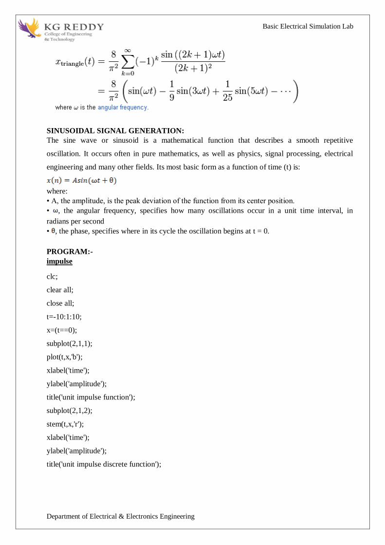
Basic Electrical Simulation Lab
Department of Electrical amp Electronics Engineering
SINUSOIDAL SIGNAL GENERATION
The sine wave or sinusoid is a mathematical function that describes a smooth repetitive
oscillation It occurs often in pure mathematics as well as physics signal processing electrical
engineering and many other fields Its most basic form as a function of time (t) is
where
bull A the amplitude is the peak deviation of the function from its center position
bull the angular frequency specifies how many oscillations occur in a unit time interval in
radians per second
bull the phase specifies where in its cycle the oscillation begins at t = 0
PROGRAM-
impulse
clc
clear all
close all
t=-10110
x=(t==0)
subplot(211)
plot(txb)
xlabel(time)
ylabel(amplitude)
title(unit impulse function)
subplot(212)
stem(txr)
xlabel(time)
ylabel(amplitude)
title(unit impulse discrete function)
Basic Electrical Simulation Lab
Department of Electrical amp Electronics Engineering
Step
clc
clear all
close all
N=100
t=1100
x=ones(1N)
subplot(211)
plot(txr)
xlabel(time)
ylabel(amplitude)
title(unit step function)
subplot(212)
stem(txr)
xlabel(time)
ylabel(amplitude)
title(unit step discrete function)
Ramp
clc
clear all
close all
t=020
x=t
subplot(211)
plot(txr)
xlabel(time)
ylabel(amplitude)
title(unit ramp function)
subplot(212)
stem(txr)
xlabel(time)
ylabel(amplitude)
title(unit ramp discrete function)
Basic Electrical Simulation Lab
Department of Electrical amp Electronics Engineering
Sinusoidal
clc
clear all
close all
t=0000012
x=sin(2pit)
subplot(211)
plot(txr)
xlabel(time)
ylabel(amplitude)
title(sinusoidal signal)
subplot(212)
stem(txr)
xlabel(time)
ylabel(amplitude)
title(sinusoidal sequence)
Square
clc
clear all
close all
t=00012
x=square(2pit)
subplot(211)
plot(txr)
xlabel(time)
ylabel(amplitude)
title(square signal)
subplot(212)
stem(txr)
xlabel(time)
ylabel(amplitude)
title(square sequence)
Basic Electrical Simulation Lab
Department of Electrical amp Electronics Engineering
Sawtooth
clc
clear all
close all
t=00012
x=sawtooth(2pi5t)
subplot(211)
plot(txk)
xlabel(time)
ylabel(amplitude)
title(sawtooth signal)
subplot(212)
stem(txr)
xlabel(time)
ylabel(amplitude)
title(sawtooth sequence)
Traingular
clc
clear all
close all
t=00012
x=sawtooth(2pi5t05)
subplot(211)
plot(txk)
xlabel(time)
ylabel(amplitude)
title(triangular signal)
subplot(212)
stem(txr)
xlabel(time)
ylabel(amplitude)
title(triangular sequence)
Basic Electrical Simulation Lab
Department of Electrical amp Electronics Engineering
Sinc
clc
clear all
close all
t=linspace(-55)
x=sinc(t)
subplot(211)
plot(txk)
xlabel(time)
ylabel(amplitude)
title(sinc signal)
subplot(212)
stem(txr)
xlabel(time)
ylabel(amplitude)
title(sinc sequence)
PROCEDURE-
1 Open OCTAVE
2 Open new script
3 Type the program
4 Save in current directory
5 Compile and Run the program
6 For the output see command window Figure window
OUTPUT-
RESULT-
Basic Electrical Simulation Lab
Department of Electrical amp Electronics Engineering
EXPERIMENT-3
OPERATIONS ON SIGNALS AND SEQUENCES SUCH AS ADDITION
MULTIPLICATION SCALING SHIFTING FOLDING COMPUTATION OF ENERGY
AND AVERAGE POWER
AIM To performs operations on signals and sequences such as addition multiplication
scaling shifting folding computation of energy and average power
APPARATUS
1 OCTAVE
2 LINUX
THEORY
Basic Operation on Signals
Time shifting y(t)=x(t-T)The effect that a time shift has on the appearance of a signal If T is a
positive number the time shifted signal x (t -T ) gets shifted to the right otherwise it gets shifted
left
Signal Shifting and Delay
Shifting y(n)=x(n-k) m=n-k y=x
Time reversal Y(t)=y(-t) Time reversal _ips the signal about t = 0 as seen in Figure
Signal Addition and Substraction
Addition any two signals can be added to form a third signal z (t) = x (t) + y (t)
Signal AmplificationAttuation
Basic Electrical Simulation Lab
Department of Electrical amp Electronics Engineering
MultiplicationDivition
Multiplication of two signals their product is also a signal z (t) = x (t) y (t)
folding
y(n)=x(-n) y=fliplr(x) n=-fliplr(n)
PROGRAM-
Addition and multiplication of two signals
clc
clear all
close all
t=000012
s1=6sin(2pi5t)
subplot(411)
plot(ts1g)
xlabel(time)
ylabel(amplitude)
title(first signal)
s2=8sin(2pi5t)
subplot(412)
plot(ts2r)
xlabel(time)
ylabel(amplitude)
title(second signal)
s3=s1+s2
subplot(413)
plot(ts3g)
xlabel(time)
ylabel(amplitude)
title(sum of two signals)
s4=s1s2
subplot(414)
plot(ts4g)
xlabel(time)
ylabel(amplitude)
title(multiplication of two signals)
Basic Electrical Simulation Lab
Department of Electrical amp Electronics Engineering
Amplitude scaling for signals
clc
clear all
close all
t=000012
s1=6sin(2pi5t)
subplot(311)
plot(ts1g)
xlabel(time)
ylabel(amplitude)
title(sinusoidal signal)
s2=3s1
subplot(312)
plot(ts2r)
xlabel(time)
ylabel(amplitude)
title(amplified signal)
s3=s13
subplot(313)
plot(ts3g)
xlabel(time)
ylabel(amplitude)
title(attenuated signal)
Time scaling for signals
clc
clear all
close all
t=000012
s1=6sin(2pi5t)
subplot(311)
plot(ts1g)
xlabel(time)
ylabel(amplitude)
title(sinusoidal signal)
t1=3t
subplot(312)
plot(t1s1r)
xlabel(time)
ylabel(amplitude)
title(compressed signal)
t2=t3
subplot(313)
plot(t2s1g)
xlabel(time)
ylabel(amplitude)
title(enlarged signal)
Basic Electrical Simulation Lab
Department of Electrical amp Electronics Engineering
Time shifting of a signal
clc
clear all
close all
t=000013
s1=6sin(2pi5t)
subplot(311)
plot(ts1g)
xlabel(time)
ylabel(amplitude)
title(sinusoidal signal)
t1=t+10
subplot(312)
plot(t1s1r)
xlabel(time)
ylabel(amplitude)
title(right shift of the signal)
t2=t-10
subplot(313)
plot(t2s1g)
xlabel(time)
ylabel(amplitude)
title(left shift of the signal)
Time folding of a signal
clc
clear all
close all
t=000012
s=sin(2pi5t)
m=length(s)
n=[-mm]
y=[0zeros(1m)s]
subplot(211)
plot(nyg)
xlabel(time)
ylabel(amplitude)
title(original signal)
y1=[fliplr(s)0zeros(1m)]
subplot(212)
plot(ny1r)
xlabel(time)
ylabel(amplitude)
title(folded signal)
Basic Electrical Simulation Lab
Department of Electrical amp Electronics Engineering
PROCEDURE-
1 Open OCTAVE
2 Open new script
3 Type the program
4 Save in current directory
5 Compile and Run the program
6 For the output see command window Figure window
OUTPUT-
RESULT-
Basic Electrical Simulation Lab
Department of Electrical amp Electronics Engineering
EXPERIMENT-4
MESH AND NODAL ANALYSIS OF ELECTRICAL CIRCUITS
AIM To Simulate the DC Circuit for determining the all node voltages and mesh currents using
NGPSPICE
APPARATUS
1 NGSPICE
2 LINUX
THEORY
NODAL ANALYSIS
In electric circuits analysis nodal analysis node-voltage analysis or the branch current
method is a method of determining the voltage (potential difference) between nodes (points
where elements or branches connect) in an electrical circuit in terms of the branch currents In
analyzing a circuit using Kirchhoffs circuit laws one can either do nodal analysis using
Kirchhoffs current law (KCL) or mesh analysis using Kirchhoffs voltage law (KVL) Nodal
analysis writes an equation at each electrical node requiring that the branch currents incident at a
node must sum to zero The branch currents are written in terms of the circuit node voltages As a
consequence each branch constitutive relation must give current as a function of voltage
an admittance representation For instance for a resistor Ibranch = Vbranch G where G (=1R) is
the admittance (conductance) of the resistor
Nodal analysis is possible when all the circuit elements branch constitutive relations have
an admittance representation Nodal analysis produces a compact set of equations for the network
which can be solved by hand if small or can be quickly solved using linear algebra by computer
Because of the compact system of equations many circuit simulation programs (eg SPICE) use
nodal analysis as a basis When elements do not have admittance representations a more general
extension of nodal analysis modified nodal analysis can be used
MESH ANALYSIS
Mesh analysis works by arbitrarily assigning mesh currents in the essential meshes (also referred
to as independent meshes) An essential mesh is a loop in the circuit that does not contain any
other loop Figure 1 labels the essential meshes with one two and three A mesh current is a
current that loops around the essential mesh and the equations are set solved in terms of them A
Basic Electrical Simulation Lab
Department of Electrical amp Electronics Engineering
mesh current may not correspond to any physically flowing current but the physical currents are
easily found from them It is usual practice to have all the mesh currents loop in the same
direction This helps prevent errors when writing out the equations The convention is to have all
the mesh currents looping in a clockwise direction
Solving for mesh currents instead of directly applying Kirchhoffs current law and Kirchhoffs
voltage law can greatly reduce the amount of calculation required This is because there are fewer
mesh currents than there are physical branch currents
CIRCUIT DIAGRAM
PROGRAM
Vs 1 0 DC 20V
Ra 1 2 5k
Rb 2 0 4k
Rc 3 0 1k
Is 3 2 DC 20mA
DC
end
OUTPUT-
RESULT-
Basic Electrical Simulation Lab
Department of Electrical amp Electronics Engineering
EXPERIMENT-5
APPLICATION OF NETWORK THEOREMS TO ELECTRICAL NETWORKS
AIM To Simulate the different network theorems to electrical networks using NGPSPICE
APPARATUS
1 NGSPICE
2 LINUX
THEORY
THEVENINrsquoS THEOREM
The Theveninrsquos Theorem states that ldquoAny two terminals linear bilateral DC network can
be replaced by an equivalent circuit consisting of a voltage source Vth in series with all equivalent
resistance Rthrdquo
(OR)
Thevenins theorem states that ldquoin any two terminal linear bilateral network having a
number of voltage current sources and resistances can be replaced by a simple equivalent circuit
consisting of a single voltage source in series with a resistance where the value of the voltage
source is equal to the open circuit voltage across the two terminals of the network and the
resistance is the equivalent resistance measured between the terminals with all energy sources
replaced by their internal resistancesrdquo
NORTONrsquoS THEOREM
Nortons theorem States that ldquoin any two terminal linear bilateral network with current
sources voltage sources and resistances can be replaced by an equivalent circuit consisting of a
current source in parallel with a resistance The value of the current source is the short circuit
current between the two terminals of the network and the resistance is the equivalent resistance
measured between the terminals of the network with all the energy sources replaced by their
internal resistancesrdquo
SUPERPOSITION THEOREM
This theorem states that ldquoThe response (voltage or current) in any branch of a bilateral
linear circuit having more than one independent source equals the algebraic sum of the responses
caused by each independent source acting alone where all the other independent sources are
replaced by their internal resistancerdquo
Basic Electrical Simulation Lab
Department of Electrical amp Electronics Engineering
i1 2kΩ
+
5000
+
minus minus
+
100i1 20kΩ
minus
1 3
2
A given response in a network regulating from a number of independent sources(including
initial condition source) may be computed by summing the response to each individual source
with all other sources made in operative( reduced to zero voltage or zero current)
This statement describes the property homogeneity in linear networks So it is the
combined properties off additivity and homogeneity off linear network It is a result of the linear
relation between current and volt in circuits having linear impedances
MAX POWER TRANSFER THEOREM
Max power will be delivered by network to the load if the impedance of network is
Complex conjugate of load impedance and vice versa
(or)
The maximum transformer states that ldquoA load will received maximum power from a
linear bilateral network when its load resistance is exactly equal to the Theveninrsquos resistance
of network measured looking back into the terminals of network
PROGRAM
THEVENINS THEORM
2mV -
Find Thevenin equivalent circuit
V10 1 0 2M V
R12 1 1A 2K
V1A 1A 2 DC 0V
E20 2 0 3 0 2E-4
F30 3 0 V1A 100
R30 3 0 20K
RL 3 0 1G
TF v(3) v10
END
NODE VOLTAGE NODE VOLTAGE NODE VOLTAGE NODE VOLTAGE
Basic Electrical Simulation Lab
Department of Electrical amp Electronics Engineering
NORTONS THEORM
PROGRAM
Vs 1 0 DC 20V
R1 1 2 18k
Rb 2 0 22k
Rc 2 3 33k
Is 3 0 RL
DC
end
MAXIMUM POWER TRANSFER THEOREM
PROGRAM
VS 1 0 DC 100
R1 1 2 10
R2 2 0 30
R3 1 3 20
R4 3 0 40
RL 2 3 RLOAD 1
MODEL RLOAD RES(R=25)
DC RES RLOAD(R) 0001 40 001
TF V(23) VS
PROBE
END
Basic Electrical Simulation Lab
Department of Electrical amp Electronics Engineering
SUPERPOSITION THEOREM
Program FOR CIRCUIT 1 FOR CIRCUIT 2
VDC 1 2 DC 10V VDC 1 2 DC 10V VDC 1 2 DC 0V
R1 1 3 100 R1 1 3 100 R1 1 3 100
R2 3 4 200 R2 3 4 200 R2 3 4 200
R3 3 6 470 R3 3 6 470 R3 3 6 470
R4 2 0 560 R4 2 0 560 R4 2 0 560
R5 4 5 100 R5 4 0 100 R5 4 5 100
VX 5 0 DC 10V VY 6 0 DC 0V VY 6 0 DC 0V
VY 6 0 DC 0V OP OP
OP END END
END
OUTPUT-
RESULT-
Basic Electrical Simulation Lab
Department of Electrical amp Electronics Engineering
EXPERIMET-6
WAVEFORM SYNTHESIS USING LAPLACE TRANSFORM
AIM To perform waveform synthesis using Laplace Transforms of a given signal
APPARATUS
1 OCTAVE
2 LINUX
THEORY
Bilateral Laplace transform
When one says the Laplace transform without qualification the unilateral or one-sided
transform is normally intended The Laplace transform can be alternatively defined as the bilateral
Laplace transform or two-sided Laplace transform by extending the limits of integration to be the
entire real axis If that is done the common unilateral transform simply becomes a special case of
the bilateral transform where the definition of the function being transformed is multiplied by the
Heaviside step function The bilateral Laplace transform is defined as follows
Inverse Laplace transform
The inverse Laplace transform is given by the following complex integral which is known by
various names (the Bromwich integral the Fourier-Mellin integral and Mellins inverse formula)
Example
Let y(t)=exp(t)
We have
The integral converges if sgt1 The functions exp(t) and 1(s-1) are partner functions
Basic Electrical Simulation Lab
Department of Electrical amp Electronics Engineering
PROGRAM-
Laplace Transform
clc
clear all
close all
syms t
x=exp(-2t)heaviside(t)
y=laplace(x)
disp(Laplace Transform of input signal)
y
z=ilaplace(y)
disp(Inverse Laplace Transform of input signal)
z
PROCEDURE-
1 Open OCTAVE
2 Open new script
3 Type the program
4 Save in current directory
5 Compile and Run the program
6 For the output see command window Figure window
OUTPUT-
RESULT-
Basic Electrical Simulation Lab
Department of Electrical amp Electronics Engineering
EXPERIMENT-7
LOCATING THE ZEROS AND POLES AND PLOTTING THE
POLE ZERO MAPS IN S-PLANE AND Z-PLANE FOR THE GIVEN
TRANSFER FUNCTION
AIM To locating the zeros and poles and plotting the pole zero maps in s-plane and z-plane
for the given transfer function
APPARATUS
1 OCTAVE
2 LINUX
THEORY
A Transfer Function is the ratio of the output of a system to the input of a system in the Laplace
domain considering its initial conditions to be zero If we have an input function of X(s) and an
output function Y(s) we define the transfer function H(s) to be
transfer function is the Laplace transform of a system‟ s impulse response
Given a continuous-time transfer function in the Laplace domain H(s) or a discrete-time one in
the Z-domain H(z) a zero is any value of s or z such that the transfer function is zero and a pole
is any value of s or z such that the transfer function is infinite
Zeros1 The value(s) for z where the numerator of the transfer function equals zero 2 The
complex frequencies that make the overall gain of the filter transfer function zero
Poles 1 The value(s) for z where the denominator of the transfer function equals zero 2 The
omplex frequencies that make the overall gain of the filter transfer function
infinite
Z-transforms
the Z-transform converts a discrete time-domain signal which is a sequence of real or complex
numbers into a complex frequency-domain representationThe Z-transform like many other
integral transforms can be defined as either a one-sided or two-sided transform
Basic Electrical Simulation Lab
Department of Electrical amp Electronics Engineering
Bilateral Z-transform
The bilateral or two-sided Z-transform of a discrete-time signal x[n] is the function X(z)
defined as
Unilateral Z-transform
Alternatively in cases where x[n] is defined only for n ge 0 the single-sided or unilateral
Z-transform is defined as
In signal processing this definition is used when the signal is causal
The roots of the equation P(z) = 0 correspond to the zeros of X(z)
The roots of the equation Q(z) = 0 correspond to the poles of X(z)
PROGRAM-
locating poles of zero on s-plane
clc
clear all
close all
num=input(enter numerator co-efficients)
den=input(enter denominator co-efficients)
h=tf(numden)
poles=roots(den)
zeros=roots(num)
sgrid
pzmap(h)
grid on
title(locating poles of zeros on s-plane)
Basic Electrical Simulation Lab
Department of Electrical amp Electronics Engineering
locating poles ampzeros on z-plane
clc
clear all
close all
num=input(enter numerator coefficient)
den=input(enter denominator coefficient)
p=roots(den)
z=roots(num)
zplane(pz)
grid
title(locating poler and zeros on s-plane)
PROCEDURE-
1 Open OCTAVE
2 Open new script
3 Type the program
4 Save in current directory
5 Compile and Run the program
6 For the output see command window Figure window
OUTPUT-
RESULT-
Basic Electrical Simulation Lab
Department of Electrical amp Electronics Engineering
EXPERIMENT-8
SIMULATION OF DC CIRCUITS
AIM To Simulate the DC network using PSPICE
APPARATUS
1 NGSPICE
2 LINUX
THEORY
Generally speaking network analysis is any structured technique used to mathematically
analyze a circuit (a ldquonetworkrdquo of interconnected components) Quite often the technician or
engineer will encounter circuits containing multiple sources of power or component
configurations which defy simplification by seriesparallel analysis techniques In those cases he
or she will be forced to use other means This chapter presents a few techniques useful in
analyzing such complex circuits
To analyse the above circuit one would first find the equivalent of R2 and R3 in parallel
then add R1 in series to arrive at a total resistance Then taking the voltage of battery B1 with
that total circuit resistance the total current could be calculated through the use of Ohmrsquos
Law (I=ER) then that current figure used to calculate voltage drops in the circuit All in all a
fairly simple procedure However the addition of just one more battery could change all of that
PROGRAM
Basic Electrical Simulation Lab
Department of Electrical amp Electronics Engineering
Vs 1 0 DC 20V
Ra 1 2 5k
Rb 2 0 4k
Rc 3 0 1k
Is 3 2 DC 20mA
DC
end
OUTPUT-
RESULT-
Basic Electrical Simulation Lab
Department of Electrical amp Electronics Engineering
EXPERIMENT-9
TRANSIENT ANALYSIS
AIM To find out the transient response by simulation of RLC circuits Using NGSPICE
APPARATUS
1 NGSPICE
2 LINUX
THEORY
The transient simulation is the calculation of a networks response on arbitrary excitations The
results are network quantities (branch currents and node voltages) as a function of time
Substantial for the transient analysis is the consideration of energy storing components ie
inductors and capacitorsThe relations between current and voltage of ideal capacitors and
inductors are given by
(61)
Or in terms of differential equations
(62)
To calculate these quantities in a computer program numerical integration methods are required
With the current-voltage relations of these components at hand it is possible to apply the modified
nodal analysis algorithm in order to calculate the networks response This means the transient
analysis attempts to find an approximation to the analytical solution at discrete time points using
numeric integration
CIRCUIT DIAGRAM
Basic Electrical Simulation Lab
Department of Electrical amp Electronics Engineering
PROGRAM
VIN1 1 0 PWL(0 0 1NS 1V 1MS 1V)
VIN2 4 0 PWL(0 0 1NS 1V 1MS 1V)
VIN3 7 0 PWL(0 0 1NS 1V 1MS 1V)
R1 1 2 2
R2 4 5 1
R3 7 8 8
L1 2 3 50UH
L2 5 6 50UH
L3 8 9 50UH
C1 3 0 10UF
C2 6 0 10UF
C3 9 0 10UF
TRAN 1US 400US
PLOT TRAN V(3) V(6) V(9)
PROBE
END
OUTPUT-
RESULT-
Basic Electrical Simulation Lab
Department of Electrical amp Electronics Engineering
EXPERIMENT-10
SIMULATION OF SINGLE PHASE DIODE BRIDGE RECTIFIERS WITH FILTER FOR
R amp RL LOAD
AIM To analyze the simulation of 1-Oslash diode bridge rectifiers with filter for R amp RL load using
NGSPICE
APPARATUS
1 NGSPICE
2 LINUX
THEORY
A bridge rectifier circuit is a common part of the electronic power supplies
Many electronic circuits require rectified DC power supply for powering the various electronic
basic components from available AC mains supply We can find this rectifier in a wide variety of
electronic AC power devices like home appliances motor controllers modulation process
welding applications etc
A Bridge rectifier is an Alternating Current (AC) to Direct Current (DC) converter that
rectifies mains AC input to DC output Bridge Rectifiers are widely used in power supplies that
provide necessary DC voltage for the electronic components or devices They can be constructed
with four or more diodes or any other controlled solid state switches Depending on the load
current requirements a proper bridge rectifier is selected Componentsrsquo ratings and specifications
breakdown voltage temperature ranges transient current rating forward current rating mounting
requirements and other considerations are taken into account while selecting a rectifier power
supply for an appropriate electronic circuitrsquos application
Bride rectifiers are classified into several types based on these factors type of supply
controlling capability bride circuitrsquos configurations etc Bridge rectifiers are mainly classified
into single and three phase rectifiers Both these types are further classified into uncontrolled half
controlled and full controlled rectifiers
Basic Electrical Simulation Lab
Department of Electrical amp Electronics Engineering
Program
VS 1 0 SIN(0 1697V 60HZ)
DF 5 4 DMOD
R1 4 7 10
L1 7 8 20MH
C1 4 6 793UF
RX 6 5 01
VX 8 5 DC 10V
VY 2 1 DC 0V
D1 2 4 DMOD
D2 5 3 DMOD
D3 3 4 DMOD
D4 5 2 DMOD
MODEL DMOD D( IS=22E-15 BV=1800 TT=0)
TRAN 10US 100MS 166MS
PROBE
FOUR 120HZ I(VX)
END
OUTPUT-
RESULT-
Basic Electrical Simulation Lab
Department of Electrical amp Electronics Engineering
EXPERIMENT-11
SIMULATION OF THREE PHASE DIODE BRIDGE RECTIFIERS WITH R RL LOAD
AIM To analyze the simulation of 3-Oslash diode bridge rectifiers with filter for R amp RL load using
NGSPICE
APPARATUS
1 NGSPICE
2 LINUX
THEORY
Three phase half controlled bridge converters amp fully controlled bridge converters are used
extensively in industrial applications up to about 15kW of output power The Three phase
controlled rectifiers provide a maximum dc output of
vdc(max)=2vm prod
The output ripple frequency is equal to the twice the ac supply frequency The single phase
full wave controlled rectifiers provide two output pulses during every input supply cycle
and hence are referred to as two pulse converters
Three phase converters are 3-phase controlled rectifiers which are used to convert ac input
power supply into dc output power across the load
Features of 3-phase controlled rectifiers are
Operate from 3 phase ac supply voltage
They provide higher dc output voltage and higher dc output power
Higher output voltage ripple frequency
Filtering requirements are simplified for smoothing out load voltage and load
current
Three phase controlled rectifiers are extensively used in high power variable speed
industrial dc drives
Basic Electrical Simulation Lab
Department of Electrical amp Electronics Engineering
Program
VAN 1 0 SIN(0V 200V 50HZ 0 0 0)
VBN 2 0 SIN(0V 200V 50HZ 0 0 -120)
VCN 3 0 SIN(0V 200V 50HZ 0 0 -240)
R 7 9 20
L 9 10 55MH
VX 10 8 DC 0V
VY 1 4 DC 0V
D1 4 7 DMOD
D2 8 2 DMOD
D3 3 7 DMOD
D4 8 4 DMOD
D5 2 7 DMOD
D6 8 3 DMOD
MODEL DMOD D(IS=22E-15 BV=1800V TT=0)
TRAN 5US 50MS 2166MS
PROBE
END
OUTPUT-
RESULT-
Basic Electrical Simulation Lab
Department of Electrical amp Electronics Engineering
EXPERIMENT-12
DESIGN OF LOW PASS AND HIGH PASS FILTERS
AIM To analyze the simulation of 3-Oslash diode bridge rectifiers with filter for R amp RL load using
NGSPICE
APPARATUS
1 OCTAVE
2 LINUX
THEORY
A filter is a circuit that has designed to pass a specified band of frequencies while attenuating all
signals outside this band Active filters employ transistors or op-amps plus resistors inductors
and capacitors There are four types of filters low-pass high-pass band-pass and band-
elimination (also referred to as band-reject or notch) filters Figure 71 illustrates frequency-
response plot for the four types of filters A low-pass filter is a circuit that has a constant output
voltage from dc up to a cutoff frequency fc As the frequency increases above fc the output
voltage is attenuated (decreases) Figure 71(a) is a plot of magnitude of the output voltage of a
low-pass filter versus frequency The range of frequencies that are transmitted is known as the
pass-band The range of frequencies that are attenuated is known as the stop-band The cutoff
frequency fc is also called the 0707 frequency the 3-dB frequency the corner frequency or the
break frequency High-pass filters attenuate the output voltage for all frequencies below the cutoff
frequency fc Above fc the magnitude of the output voltage is constant Figure 71(b) is the plot
for ideal and practical high-pass filters Band-pass filters pass only a band of frequencies while
attenuating all frequencies outside the band Band-elimination filters perform in an exactly
opposite way that is band-elimination filters reject a specified band of frequencies while passing
all frequencies outside the band Typical frequency-response plots for band-pass and band-
elimination filters are shown in Figure 71(c) and (d) In many filter applications it is necessary
for the closed-loop gain to be as close to 1 as possible within the pass band The Butterworth filter
is best suited for this type of application The Butterworth filter is also called a maximally flat or
flat-flat filter and all filter in this experiment will be of the Butterworth type Figure 72 shows
the ideal and the practical frequency response for three types of Butterworth filters As the roll-
offs become steeper they approach the ideal filter more closely
Basic Electrical Simulation Lab
Department of Electrical amp Electronics Engineering
PROGRAM
LOW PASS FILTER
N = 100 FIR filter order
Fp = 20e3 20 kHz passband-edge frequency
Fs = 96e3 96 kHz sampling frequency
Rp = 000057565 Corresponds to 001 dB peak-to-peak ripple
Rst = 1e-4 Corresponds to 80 dB stopband attenuation
eqnum = firceqrip(NFp(Fs2)[Rp Rst]passedge) eqnum = vec of coeffs
fvtool(eqnumFsFsColorWhite) Visualize filter
HIGH PASS FILTER
Fstop = 350
Fpass = 400
Astop = 65
Apass = 05
Fs = 1e3
d = designfilt(highpassfirStopbandFrequencyFstop
PassbandFrequencyFpassStopbandAttenuationAstop
PassbandRippleApassSampleRateFsDesignMethodequiripple)
fvtool(d)
OUTPUT-
RESULT-
Basic Electrical Simulation Lab
Department of Electrical amp Electronics Engineering
EXPERIMENT-13
FINDING THE EVEN AND ODD PARTS OF SIGNAL SEQUENCE AND REAL AND
IMAGINARY PARTS OF SIGNAL
AIM
program for finding even and odd parts of sequences Using OCTAVE Softwareamp
program for finding real and imaginary parts of sequences Using OCTAVE Software
APPARATUS
1 OCTAVE
2 LINUX
THEORY
Even and Odd Signal
One of characteristics of signal is symmetry that may be useful for signal analysis Even signals
are symmetric around vertical axis and Odd signals are symmetric about origin
Even Signal A signal is referred to as an even if it is identical to its time-reversed counterparts
x(t) = x(-t)
Odd Signal A signal is odd if x(t) = -x(-t)
An odd signal must be 0 at t=0 in other words odd signal passes the origin
Using the definition of even and odd signal any signal may be decomposed into a sum of its even
part xe(t) and its odd part xo(t) as follows
x(t)=xe(t)+xo(t)
x(t)=12x(t)+x(-t) +12x(t)-x(-t)
where
xe(t)=12x(t)+x(-t) ampxo(t)=12x(t)-x(-t)
It is an important fact because it is relative concept of Fourier series In Fourier series aperiodic
signal can be broken into a sum of sine and cosine signals Notice that sine function is odd signal
and cosine function is even signal
ENERGY AND POWER SIGNAL
A signal can be categorized into energy signal or power
signal An energy signal has a finite energy 0 lt E lt 1049279 In other words energy signals have
values only in the limited time duration For example a signal having only one square pulse is
energy signal A signal that decays exponentially has finite energy so it is also an energy signal
The power of an energy signal is 0 because of dividing finite energy by infinite time (or length)
If x(t) is a real-valued signal with Fourier transform X(f) and u(f) is the Heaviside step function
Basic Electrical Simulation Lab
Department of Electrical amp Electronics Engineering
then the function
contains only the non-negative frequency components of X(f) And the operation is reversible due
to the Hermitian property of X(f)
X(f) denotes the complex conjugate of X(f)
The inverse Fourier transform of Xa(f) is the analytic signal
where x^(t) is the Hilbert transform of x(t) and J is the imaginary unit
Basic Electrical Simulation Lab
Department of Electrical amp Electronics Engineering
PROGRAM-
Evenoddrealimaginary parts of a sequences
clc
clear all
close all
h=input(enter noof samples)
m=(h-1)2
n=-mm
x=input(enter sample values)
subplot(411)
stem(nxg)
xlabel(time)
ylabel(amplitude)
title(original sequence)
xmir=fliplr(x)
subplot(412)
stem(nxmirr)
xlabel(time)
ylabel(amplitude)
title(folded sequence)
even part of sequence
xeven=(x+xmir)2
subplot(413)
stem(nxevenr)
xlabel(time)
ylabel(amplitude)
title(even part of sequence)
odd part of sequence
xodd=(x-xmir)2
subplot(414)
stem(nxoddg)
xlabel(time)
ylabel(amplitude)
title(odd part of sequence)
Basic Electrical Simulation Lab
Department of Electrical amp Electronics Engineering
RealampImaginary parts of a sequences
clc
clear all
close all
y=input(enter complex numbers)
yreal=real(y)
disp(real values of y)
yreal
yimag=imag(y)
disp(imaginary values of y)
yimag
PROCEDURE-
1 Open OCTAVE
2 Open new script
3 Type the program
4 Save in current directory
5 Compile and Run the program
6 For the output see command window Figure window
OUTPUT-
RESULT-
Basic Electrical Simulation Lab
Department of Electrical amp Electronics Engineering
EXPERIMENT-14
FINDING THE FOURIER TRANSFORM OF A GIVEN SIGNAL AND PLOTTING ITS
MAGNITUDE AND PHASE SPECTRUM
AIM
Program for finding the fourier transform of a given signal Using OCTAVE Software amp Plotting
Its Magnitude And Phase Spectrum Using OCTAVE Software
APPARATUS
1 OCTAVE
2 LINUX
THEORY
The Fourier transform (FT) decomposes a function of time (a signal) into the
frequencies that make it up in a way similar to how a musical chord can be expressed as the
frequencies (or pitches) of its constituent notes The Fourier transform of a function of time itself
is a complex-valued function of frequency whose absolute value represents the amount of that
frequency present in the original function and whose complex argument is the phase offset of the
basic sinusoid in that frequency The Fourier transform is called the frequency domain
representation of the original signal The term Fourier transform refers to both the frequency
domain representation and the mathematical operation that associates the frequency domain
representation to a function of time The Fourier transform is not limited to functions of time but
in order to have a unified language the domain of the original function is commonly referred to as
the time domain For many functions of practical interest one can define an operation that
reverses this the inverse Fourier transformation also called Fourier synthesis of a frequency
domain representation combines the contributions of all the different frequencies to recover the
original function of time
Linear operations performed in one domain (time or frequency) have corresponding
operations in the other domain which are sometimes easier to perform The operation
of differentiation in the time domain corresponds to multiplication by the frequency[remark 1] so
some differential equations are easier to analyze in the frequency domain Also convolution in the
time domain corresponds to ordinary multiplication in the frequency domain Concretely this
means that any linear time-invariant system such as a filter applied to a signal can be expressed
relatively simply as an operation on frequencies After performing the desired operations
transformation of the result can be made back to the time domain Harmonic analysis is the
systematic study of the relationship between the frequency and time domains including the kinds
Basic Electrical Simulation Lab
Department of Electrical amp Electronics Engineering
of functions or operations that are simpler in one or the other and has deep connections to many
areas of modern mathematics
PROGRAM
Fs = 1000 Sampling frequency
T = 1Fs Sampling period
L = 1500 Length of signal
t = (0L-1)T Time vector
S = 07sin(2pi50t) + sin(2pi120t)
X = S + 2randn(size(t))
plot(1000t(150)X(150))
title(Signal Corrupted with Zero-Mean Random Noise)
xlabel(t (milliseconds))
ylabel(X(t))
Y = fft(X)
P2 = abs(YL)
P1 = P2(1L2+1)
P1(2end-1) = 2P1(2end-1)
f = Fs(0(L2))L
plot(fP1)
title(Single-Sided Amplitude Spectrum of X(t))
xlabel(f (Hz))
ylabel(|P1(f)|)
Y = fft(S)
P2 = abs(YL)
P1 = P2(1L2+1)
P1(2end-1) = 2P1(2end-1)
plot(fP1)
title(Single-Sided Amplitude Spectrum of S(t))
xlabel(f (Hz))
ylabel(|P1(f)|)
OUTPUT-
RESULT-
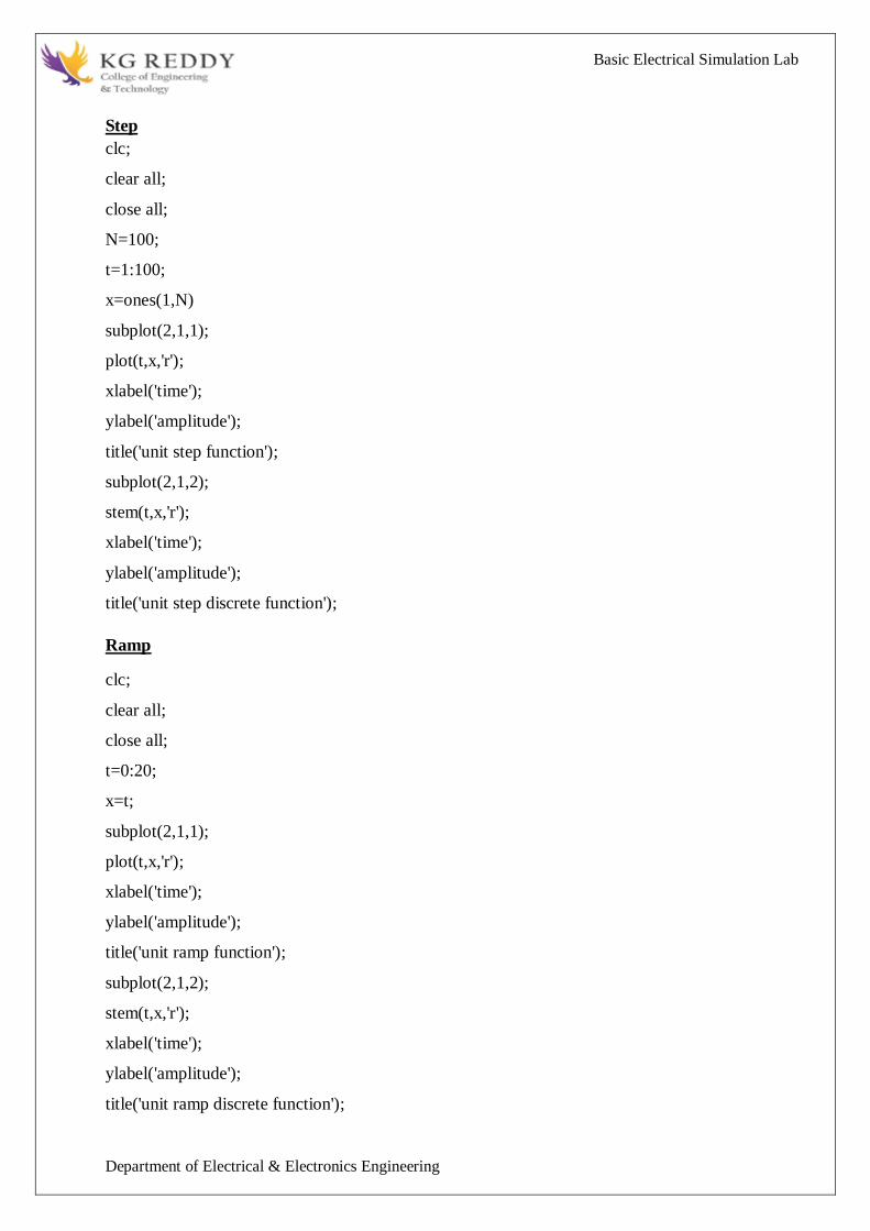
Basic Electrical Simulation Lab
Department of Electrical amp Electronics Engineering
Sinusoidal
clc
clear all
close all
t=0000012
x=sin(2pit)
subplot(211)
plot(txr)
xlabel(time)
ylabel(amplitude)
title(sinusoidal signal)
subplot(212)
stem(txr)
xlabel(time)
ylabel(amplitude)
title(sinusoidal sequence)
Square
clc
clear all
close all
t=00012
x=square(2pit)
subplot(211)
plot(txr)
xlabel(time)
ylabel(amplitude)
title(square signal)
subplot(212)
stem(txr)
xlabel(time)
ylabel(amplitude)
title(square sequence)
Basic Electrical Simulation Lab
Department of Electrical amp Electronics Engineering
Sawtooth
clc
clear all
close all
t=00012
x=sawtooth(2pi5t)
subplot(211)
plot(txk)
xlabel(time)
ylabel(amplitude)
title(sawtooth signal)
subplot(212)
stem(txr)
xlabel(time)
ylabel(amplitude)
title(sawtooth sequence)
Traingular
clc
clear all
close all
t=00012
x=sawtooth(2pi5t05)
subplot(211)
plot(txk)
xlabel(time)
ylabel(amplitude)
title(triangular signal)
subplot(212)
stem(txr)
xlabel(time)
ylabel(amplitude)
title(triangular sequence)
Basic Electrical Simulation Lab
Department of Electrical amp Electronics Engineering
Sinc
clc
clear all
close all
t=linspace(-55)
x=sinc(t)
subplot(211)
plot(txk)
xlabel(time)
ylabel(amplitude)
title(sinc signal)
subplot(212)
stem(txr)
xlabel(time)
ylabel(amplitude)
title(sinc sequence)
PROCEDURE-
1 Open OCTAVE
2 Open new script
3 Type the program
4 Save in current directory
5 Compile and Run the program
6 For the output see command window Figure window
OUTPUT-
RESULT-
Basic Electrical Simulation Lab
Department of Electrical amp Electronics Engineering
EXPERIMENT-3
OPERATIONS ON SIGNALS AND SEQUENCES SUCH AS ADDITION
MULTIPLICATION SCALING SHIFTING FOLDING COMPUTATION OF ENERGY
AND AVERAGE POWER
AIM To performs operations on signals and sequences such as addition multiplication
scaling shifting folding computation of energy and average power
APPARATUS
1 OCTAVE
2 LINUX
THEORY
Basic Operation on Signals
Time shifting y(t)=x(t-T)The effect that a time shift has on the appearance of a signal If T is a
positive number the time shifted signal x (t -T ) gets shifted to the right otherwise it gets shifted
left
Signal Shifting and Delay
Shifting y(n)=x(n-k) m=n-k y=x
Time reversal Y(t)=y(-t) Time reversal _ips the signal about t = 0 as seen in Figure
Signal Addition and Substraction
Addition any two signals can be added to form a third signal z (t) = x (t) + y (t)
Signal AmplificationAttuation
Basic Electrical Simulation Lab
Department of Electrical amp Electronics Engineering
MultiplicationDivition
Multiplication of two signals their product is also a signal z (t) = x (t) y (t)
folding
y(n)=x(-n) y=fliplr(x) n=-fliplr(n)
PROGRAM-
Addition and multiplication of two signals
clc
clear all
close all
t=000012
s1=6sin(2pi5t)
subplot(411)
plot(ts1g)
xlabel(time)
ylabel(amplitude)
title(first signal)
s2=8sin(2pi5t)
subplot(412)
plot(ts2r)
xlabel(time)
ylabel(amplitude)
title(second signal)
s3=s1+s2
subplot(413)
plot(ts3g)
xlabel(time)
ylabel(amplitude)
title(sum of two signals)
s4=s1s2
subplot(414)
plot(ts4g)
xlabel(time)
ylabel(amplitude)
title(multiplication of two signals)
Basic Electrical Simulation Lab
Department of Electrical amp Electronics Engineering
Amplitude scaling for signals
clc
clear all
close all
t=000012
s1=6sin(2pi5t)
subplot(311)
plot(ts1g)
xlabel(time)
ylabel(amplitude)
title(sinusoidal signal)
s2=3s1
subplot(312)
plot(ts2r)
xlabel(time)
ylabel(amplitude)
title(amplified signal)
s3=s13
subplot(313)
plot(ts3g)
xlabel(time)
ylabel(amplitude)
title(attenuated signal)
Time scaling for signals
clc
clear all
close all
t=000012
s1=6sin(2pi5t)
subplot(311)
plot(ts1g)
xlabel(time)
ylabel(amplitude)
title(sinusoidal signal)
t1=3t
subplot(312)
plot(t1s1r)
xlabel(time)
ylabel(amplitude)
title(compressed signal)
t2=t3
subplot(313)
plot(t2s1g)
xlabel(time)
ylabel(amplitude)
title(enlarged signal)
Basic Electrical Simulation Lab
Department of Electrical amp Electronics Engineering
Time shifting of a signal
clc
clear all
close all
t=000013
s1=6sin(2pi5t)
subplot(311)
plot(ts1g)
xlabel(time)
ylabel(amplitude)
title(sinusoidal signal)
t1=t+10
subplot(312)
plot(t1s1r)
xlabel(time)
ylabel(amplitude)
title(right shift of the signal)
t2=t-10
subplot(313)
plot(t2s1g)
xlabel(time)
ylabel(amplitude)
title(left shift of the signal)
Time folding of a signal
clc
clear all
close all
t=000012
s=sin(2pi5t)
m=length(s)
n=[-mm]
y=[0zeros(1m)s]
subplot(211)
plot(nyg)
xlabel(time)
ylabel(amplitude)
title(original signal)
y1=[fliplr(s)0zeros(1m)]
subplot(212)
plot(ny1r)
xlabel(time)
ylabel(amplitude)
title(folded signal)
Basic Electrical Simulation Lab
Department of Electrical amp Electronics Engineering
PROCEDURE-
1 Open OCTAVE
2 Open new script
3 Type the program
4 Save in current directory
5 Compile and Run the program
6 For the output see command window Figure window
OUTPUT-
RESULT-
Basic Electrical Simulation Lab
Department of Electrical amp Electronics Engineering
EXPERIMENT-4
MESH AND NODAL ANALYSIS OF ELECTRICAL CIRCUITS
AIM To Simulate the DC Circuit for determining the all node voltages and mesh currents using
NGPSPICE
APPARATUS
1 NGSPICE
2 LINUX
THEORY
NODAL ANALYSIS
In electric circuits analysis nodal analysis node-voltage analysis or the branch current
method is a method of determining the voltage (potential difference) between nodes (points
where elements or branches connect) in an electrical circuit in terms of the branch currents In
analyzing a circuit using Kirchhoffs circuit laws one can either do nodal analysis using
Kirchhoffs current law (KCL) or mesh analysis using Kirchhoffs voltage law (KVL) Nodal
analysis writes an equation at each electrical node requiring that the branch currents incident at a
node must sum to zero The branch currents are written in terms of the circuit node voltages As a
consequence each branch constitutive relation must give current as a function of voltage
an admittance representation For instance for a resistor Ibranch = Vbranch G where G (=1R) is
the admittance (conductance) of the resistor
Nodal analysis is possible when all the circuit elements branch constitutive relations have
an admittance representation Nodal analysis produces a compact set of equations for the network
which can be solved by hand if small or can be quickly solved using linear algebra by computer
Because of the compact system of equations many circuit simulation programs (eg SPICE) use
nodal analysis as a basis When elements do not have admittance representations a more general
extension of nodal analysis modified nodal analysis can be used
MESH ANALYSIS
Mesh analysis works by arbitrarily assigning mesh currents in the essential meshes (also referred
to as independent meshes) An essential mesh is a loop in the circuit that does not contain any
other loop Figure 1 labels the essential meshes with one two and three A mesh current is a
current that loops around the essential mesh and the equations are set solved in terms of them A
Basic Electrical Simulation Lab
Department of Electrical amp Electronics Engineering
mesh current may not correspond to any physically flowing current but the physical currents are
easily found from them It is usual practice to have all the mesh currents loop in the same
direction This helps prevent errors when writing out the equations The convention is to have all
the mesh currents looping in a clockwise direction
Solving for mesh currents instead of directly applying Kirchhoffs current law and Kirchhoffs
voltage law can greatly reduce the amount of calculation required This is because there are fewer
mesh currents than there are physical branch currents
CIRCUIT DIAGRAM
PROGRAM
Vs 1 0 DC 20V
Ra 1 2 5k
Rb 2 0 4k
Rc 3 0 1k
Is 3 2 DC 20mA
DC
end
OUTPUT-
RESULT-
Basic Electrical Simulation Lab
Department of Electrical amp Electronics Engineering
EXPERIMENT-5
APPLICATION OF NETWORK THEOREMS TO ELECTRICAL NETWORKS
AIM To Simulate the different network theorems to electrical networks using NGPSPICE
APPARATUS
1 NGSPICE
2 LINUX
THEORY
THEVENINrsquoS THEOREM
The Theveninrsquos Theorem states that ldquoAny two terminals linear bilateral DC network can
be replaced by an equivalent circuit consisting of a voltage source Vth in series with all equivalent
resistance Rthrdquo
(OR)
Thevenins theorem states that ldquoin any two terminal linear bilateral network having a
number of voltage current sources and resistances can be replaced by a simple equivalent circuit
consisting of a single voltage source in series with a resistance where the value of the voltage
source is equal to the open circuit voltage across the two terminals of the network and the
resistance is the equivalent resistance measured between the terminals with all energy sources
replaced by their internal resistancesrdquo
NORTONrsquoS THEOREM
Nortons theorem States that ldquoin any two terminal linear bilateral network with current
sources voltage sources and resistances can be replaced by an equivalent circuit consisting of a
current source in parallel with a resistance The value of the current source is the short circuit
current between the two terminals of the network and the resistance is the equivalent resistance
measured between the terminals of the network with all the energy sources replaced by their
internal resistancesrdquo
SUPERPOSITION THEOREM
This theorem states that ldquoThe response (voltage or current) in any branch of a bilateral
linear circuit having more than one independent source equals the algebraic sum of the responses
caused by each independent source acting alone where all the other independent sources are
replaced by their internal resistancerdquo
Basic Electrical Simulation Lab
Department of Electrical amp Electronics Engineering
i1 2kΩ
+
5000
+
minus minus
+
100i1 20kΩ
minus
1 3
2
A given response in a network regulating from a number of independent sources(including
initial condition source) may be computed by summing the response to each individual source
with all other sources made in operative( reduced to zero voltage or zero current)
This statement describes the property homogeneity in linear networks So it is the
combined properties off additivity and homogeneity off linear network It is a result of the linear
relation between current and volt in circuits having linear impedances
MAX POWER TRANSFER THEOREM
Max power will be delivered by network to the load if the impedance of network is
Complex conjugate of load impedance and vice versa
(or)
The maximum transformer states that ldquoA load will received maximum power from a
linear bilateral network when its load resistance is exactly equal to the Theveninrsquos resistance
of network measured looking back into the terminals of network
PROGRAM
THEVENINS THEORM
2mV -
Find Thevenin equivalent circuit
V10 1 0 2M V
R12 1 1A 2K
V1A 1A 2 DC 0V
E20 2 0 3 0 2E-4
F30 3 0 V1A 100
R30 3 0 20K
RL 3 0 1G
TF v(3) v10
END
NODE VOLTAGE NODE VOLTAGE NODE VOLTAGE NODE VOLTAGE
Basic Electrical Simulation Lab
Department of Electrical amp Electronics Engineering
NORTONS THEORM
PROGRAM
Vs 1 0 DC 20V
R1 1 2 18k
Rb 2 0 22k
Rc 2 3 33k
Is 3 0 RL
DC
end
MAXIMUM POWER TRANSFER THEOREM
PROGRAM
VS 1 0 DC 100
R1 1 2 10
R2 2 0 30
R3 1 3 20
R4 3 0 40
RL 2 3 RLOAD 1
MODEL RLOAD RES(R=25)
DC RES RLOAD(R) 0001 40 001
TF V(23) VS
PROBE
END
Basic Electrical Simulation Lab
Department of Electrical amp Electronics Engineering
SUPERPOSITION THEOREM
Program FOR CIRCUIT 1 FOR CIRCUIT 2
VDC 1 2 DC 10V VDC 1 2 DC 10V VDC 1 2 DC 0V
R1 1 3 100 R1 1 3 100 R1 1 3 100
R2 3 4 200 R2 3 4 200 R2 3 4 200
R3 3 6 470 R3 3 6 470 R3 3 6 470
R4 2 0 560 R4 2 0 560 R4 2 0 560
R5 4 5 100 R5 4 0 100 R5 4 5 100
VX 5 0 DC 10V VY 6 0 DC 0V VY 6 0 DC 0V
VY 6 0 DC 0V OP OP
OP END END
END
OUTPUT-
RESULT-
Basic Electrical Simulation Lab
Department of Electrical amp Electronics Engineering
EXPERIMET-6
WAVEFORM SYNTHESIS USING LAPLACE TRANSFORM
AIM To perform waveform synthesis using Laplace Transforms of a given signal
APPARATUS
1 OCTAVE
2 LINUX
THEORY
Bilateral Laplace transform
When one says the Laplace transform without qualification the unilateral or one-sided
transform is normally intended The Laplace transform can be alternatively defined as the bilateral
Laplace transform or two-sided Laplace transform by extending the limits of integration to be the
entire real axis If that is done the common unilateral transform simply becomes a special case of
the bilateral transform where the definition of the function being transformed is multiplied by the
Heaviside step function The bilateral Laplace transform is defined as follows
Inverse Laplace transform
The inverse Laplace transform is given by the following complex integral which is known by
various names (the Bromwich integral the Fourier-Mellin integral and Mellins inverse formula)
Example
Let y(t)=exp(t)
We have
The integral converges if sgt1 The functions exp(t) and 1(s-1) are partner functions
Basic Electrical Simulation Lab
Department of Electrical amp Electronics Engineering
PROGRAM-
Laplace Transform
clc
clear all
close all
syms t
x=exp(-2t)heaviside(t)
y=laplace(x)
disp(Laplace Transform of input signal)
y
z=ilaplace(y)
disp(Inverse Laplace Transform of input signal)
z
PROCEDURE-
1 Open OCTAVE
2 Open new script
3 Type the program
4 Save in current directory
5 Compile and Run the program
6 For the output see command window Figure window
OUTPUT-
RESULT-
Basic Electrical Simulation Lab
Department of Electrical amp Electronics Engineering
EXPERIMENT-7
LOCATING THE ZEROS AND POLES AND PLOTTING THE
POLE ZERO MAPS IN S-PLANE AND Z-PLANE FOR THE GIVEN
TRANSFER FUNCTION
AIM To locating the zeros and poles and plotting the pole zero maps in s-plane and z-plane
for the given transfer function
APPARATUS
1 OCTAVE
2 LINUX
THEORY
A Transfer Function is the ratio of the output of a system to the input of a system in the Laplace
domain considering its initial conditions to be zero If we have an input function of X(s) and an
output function Y(s) we define the transfer function H(s) to be
transfer function is the Laplace transform of a system‟ s impulse response
Given a continuous-time transfer function in the Laplace domain H(s) or a discrete-time one in
the Z-domain H(z) a zero is any value of s or z such that the transfer function is zero and a pole
is any value of s or z such that the transfer function is infinite
Zeros1 The value(s) for z where the numerator of the transfer function equals zero 2 The
complex frequencies that make the overall gain of the filter transfer function zero
Poles 1 The value(s) for z where the denominator of the transfer function equals zero 2 The
omplex frequencies that make the overall gain of the filter transfer function
infinite
Z-transforms
the Z-transform converts a discrete time-domain signal which is a sequence of real or complex
numbers into a complex frequency-domain representationThe Z-transform like many other
integral transforms can be defined as either a one-sided or two-sided transform
Basic Electrical Simulation Lab
Department of Electrical amp Electronics Engineering
Bilateral Z-transform
The bilateral or two-sided Z-transform of a discrete-time signal x[n] is the function X(z)
defined as
Unilateral Z-transform
Alternatively in cases where x[n] is defined only for n ge 0 the single-sided or unilateral
Z-transform is defined as
In signal processing this definition is used when the signal is causal
The roots of the equation P(z) = 0 correspond to the zeros of X(z)
The roots of the equation Q(z) = 0 correspond to the poles of X(z)
PROGRAM-
locating poles of zero on s-plane
clc
clear all
close all
num=input(enter numerator co-efficients)
den=input(enter denominator co-efficients)
h=tf(numden)
poles=roots(den)
zeros=roots(num)
sgrid
pzmap(h)
grid on
title(locating poles of zeros on s-plane)
Basic Electrical Simulation Lab
Department of Electrical amp Electronics Engineering
locating poles ampzeros on z-plane
clc
clear all
close all
num=input(enter numerator coefficient)
den=input(enter denominator coefficient)
p=roots(den)
z=roots(num)
zplane(pz)
grid
title(locating poler and zeros on s-plane)
PROCEDURE-
1 Open OCTAVE
2 Open new script
3 Type the program
4 Save in current directory
5 Compile and Run the program
6 For the output see command window Figure window
OUTPUT-
RESULT-
Basic Electrical Simulation Lab
Department of Electrical amp Electronics Engineering
EXPERIMENT-8
SIMULATION OF DC CIRCUITS
AIM To Simulate the DC network using PSPICE
APPARATUS
1 NGSPICE
2 LINUX
THEORY
Generally speaking network analysis is any structured technique used to mathematically
analyze a circuit (a ldquonetworkrdquo of interconnected components) Quite often the technician or
engineer will encounter circuits containing multiple sources of power or component
configurations which defy simplification by seriesparallel analysis techniques In those cases he
or she will be forced to use other means This chapter presents a few techniques useful in
analyzing such complex circuits
To analyse the above circuit one would first find the equivalent of R2 and R3 in parallel
then add R1 in series to arrive at a total resistance Then taking the voltage of battery B1 with
that total circuit resistance the total current could be calculated through the use of Ohmrsquos
Law (I=ER) then that current figure used to calculate voltage drops in the circuit All in all a
fairly simple procedure However the addition of just one more battery could change all of that
PROGRAM
Basic Electrical Simulation Lab
Department of Electrical amp Electronics Engineering
Vs 1 0 DC 20V
Ra 1 2 5k
Rb 2 0 4k
Rc 3 0 1k
Is 3 2 DC 20mA
DC
end
OUTPUT-
RESULT-
Basic Electrical Simulation Lab
Department of Electrical amp Electronics Engineering
EXPERIMENT-9
TRANSIENT ANALYSIS
AIM To find out the transient response by simulation of RLC circuits Using NGSPICE
APPARATUS
1 NGSPICE
2 LINUX
THEORY
The transient simulation is the calculation of a networks response on arbitrary excitations The
results are network quantities (branch currents and node voltages) as a function of time
Substantial for the transient analysis is the consideration of energy storing components ie
inductors and capacitorsThe relations between current and voltage of ideal capacitors and
inductors are given by
(61)
Or in terms of differential equations
(62)
To calculate these quantities in a computer program numerical integration methods are required
With the current-voltage relations of these components at hand it is possible to apply the modified
nodal analysis algorithm in order to calculate the networks response This means the transient
analysis attempts to find an approximation to the analytical solution at discrete time points using
numeric integration
CIRCUIT DIAGRAM
Basic Electrical Simulation Lab
Department of Electrical amp Electronics Engineering
PROGRAM
VIN1 1 0 PWL(0 0 1NS 1V 1MS 1V)
VIN2 4 0 PWL(0 0 1NS 1V 1MS 1V)
VIN3 7 0 PWL(0 0 1NS 1V 1MS 1V)
R1 1 2 2
R2 4 5 1
R3 7 8 8
L1 2 3 50UH
L2 5 6 50UH
L3 8 9 50UH
C1 3 0 10UF
C2 6 0 10UF
C3 9 0 10UF
TRAN 1US 400US
PLOT TRAN V(3) V(6) V(9)
PROBE
END
OUTPUT-
RESULT-
Basic Electrical Simulation Lab
Department of Electrical amp Electronics Engineering
EXPERIMENT-10
SIMULATION OF SINGLE PHASE DIODE BRIDGE RECTIFIERS WITH FILTER FOR
R amp RL LOAD
AIM To analyze the simulation of 1-Oslash diode bridge rectifiers with filter for R amp RL load using
NGSPICE
APPARATUS
1 NGSPICE
2 LINUX
THEORY
A bridge rectifier circuit is a common part of the electronic power supplies
Many electronic circuits require rectified DC power supply for powering the various electronic
basic components from available AC mains supply We can find this rectifier in a wide variety of
electronic AC power devices like home appliances motor controllers modulation process
welding applications etc
A Bridge rectifier is an Alternating Current (AC) to Direct Current (DC) converter that
rectifies mains AC input to DC output Bridge Rectifiers are widely used in power supplies that
provide necessary DC voltage for the electronic components or devices They can be constructed
with four or more diodes or any other controlled solid state switches Depending on the load
current requirements a proper bridge rectifier is selected Componentsrsquo ratings and specifications
breakdown voltage temperature ranges transient current rating forward current rating mounting
requirements and other considerations are taken into account while selecting a rectifier power
supply for an appropriate electronic circuitrsquos application
Bride rectifiers are classified into several types based on these factors type of supply
controlling capability bride circuitrsquos configurations etc Bridge rectifiers are mainly classified
into single and three phase rectifiers Both these types are further classified into uncontrolled half
controlled and full controlled rectifiers
Basic Electrical Simulation Lab
Department of Electrical amp Electronics Engineering
Program
VS 1 0 SIN(0 1697V 60HZ)
DF 5 4 DMOD
R1 4 7 10
L1 7 8 20MH
C1 4 6 793UF
RX 6 5 01
VX 8 5 DC 10V
VY 2 1 DC 0V
D1 2 4 DMOD
D2 5 3 DMOD
D3 3 4 DMOD
D4 5 2 DMOD
MODEL DMOD D( IS=22E-15 BV=1800 TT=0)
TRAN 10US 100MS 166MS
PROBE
FOUR 120HZ I(VX)
END
OUTPUT-
RESULT-
Basic Electrical Simulation Lab
Department of Electrical amp Electronics Engineering
EXPERIMENT-11
SIMULATION OF THREE PHASE DIODE BRIDGE RECTIFIERS WITH R RL LOAD
AIM To analyze the simulation of 3-Oslash diode bridge rectifiers with filter for R amp RL load using
NGSPICE
APPARATUS
1 NGSPICE
2 LINUX
THEORY
Three phase half controlled bridge converters amp fully controlled bridge converters are used
extensively in industrial applications up to about 15kW of output power The Three phase
controlled rectifiers provide a maximum dc output of
vdc(max)=2vm prod
The output ripple frequency is equal to the twice the ac supply frequency The single phase
full wave controlled rectifiers provide two output pulses during every input supply cycle
and hence are referred to as two pulse converters
Three phase converters are 3-phase controlled rectifiers which are used to convert ac input
power supply into dc output power across the load
Features of 3-phase controlled rectifiers are
Operate from 3 phase ac supply voltage
They provide higher dc output voltage and higher dc output power
Higher output voltage ripple frequency
Filtering requirements are simplified for smoothing out load voltage and load
current
Three phase controlled rectifiers are extensively used in high power variable speed
industrial dc drives
Basic Electrical Simulation Lab
Department of Electrical amp Electronics Engineering
Program
VAN 1 0 SIN(0V 200V 50HZ 0 0 0)
VBN 2 0 SIN(0V 200V 50HZ 0 0 -120)
VCN 3 0 SIN(0V 200V 50HZ 0 0 -240)
R 7 9 20
L 9 10 55MH
VX 10 8 DC 0V
VY 1 4 DC 0V
D1 4 7 DMOD
D2 8 2 DMOD
D3 3 7 DMOD
D4 8 4 DMOD
D5 2 7 DMOD
D6 8 3 DMOD
MODEL DMOD D(IS=22E-15 BV=1800V TT=0)
TRAN 5US 50MS 2166MS
PROBE
END
OUTPUT-
RESULT-
Basic Electrical Simulation Lab
Department of Electrical amp Electronics Engineering
EXPERIMENT-12
DESIGN OF LOW PASS AND HIGH PASS FILTERS
AIM To analyze the simulation of 3-Oslash diode bridge rectifiers with filter for R amp RL load using
NGSPICE
APPARATUS
1 OCTAVE
2 LINUX
THEORY
A filter is a circuit that has designed to pass a specified band of frequencies while attenuating all
signals outside this band Active filters employ transistors or op-amps plus resistors inductors
and capacitors There are four types of filters low-pass high-pass band-pass and band-
elimination (also referred to as band-reject or notch) filters Figure 71 illustrates frequency-
response plot for the four types of filters A low-pass filter is a circuit that has a constant output
voltage from dc up to a cutoff frequency fc As the frequency increases above fc the output
voltage is attenuated (decreases) Figure 71(a) is a plot of magnitude of the output voltage of a
low-pass filter versus frequency The range of frequencies that are transmitted is known as the
pass-band The range of frequencies that are attenuated is known as the stop-band The cutoff
frequency fc is also called the 0707 frequency the 3-dB frequency the corner frequency or the
break frequency High-pass filters attenuate the output voltage for all frequencies below the cutoff
frequency fc Above fc the magnitude of the output voltage is constant Figure 71(b) is the plot
for ideal and practical high-pass filters Band-pass filters pass only a band of frequencies while
attenuating all frequencies outside the band Band-elimination filters perform in an exactly
opposite way that is band-elimination filters reject a specified band of frequencies while passing
all frequencies outside the band Typical frequency-response plots for band-pass and band-
elimination filters are shown in Figure 71(c) and (d) In many filter applications it is necessary
for the closed-loop gain to be as close to 1 as possible within the pass band The Butterworth filter
is best suited for this type of application The Butterworth filter is also called a maximally flat or
flat-flat filter and all filter in this experiment will be of the Butterworth type Figure 72 shows
the ideal and the practical frequency response for three types of Butterworth filters As the roll-
offs become steeper they approach the ideal filter more closely
Basic Electrical Simulation Lab
Department of Electrical amp Electronics Engineering
PROGRAM
LOW PASS FILTER
N = 100 FIR filter order
Fp = 20e3 20 kHz passband-edge frequency
Fs = 96e3 96 kHz sampling frequency
Rp = 000057565 Corresponds to 001 dB peak-to-peak ripple
Rst = 1e-4 Corresponds to 80 dB stopband attenuation
eqnum = firceqrip(NFp(Fs2)[Rp Rst]passedge) eqnum = vec of coeffs
fvtool(eqnumFsFsColorWhite) Visualize filter
HIGH PASS FILTER
Fstop = 350
Fpass = 400
Astop = 65
Apass = 05
Fs = 1e3
d = designfilt(highpassfirStopbandFrequencyFstop
PassbandFrequencyFpassStopbandAttenuationAstop
PassbandRippleApassSampleRateFsDesignMethodequiripple)
fvtool(d)
OUTPUT-
RESULT-
Basic Electrical Simulation Lab
Department of Electrical amp Electronics Engineering
EXPERIMENT-13
FINDING THE EVEN AND ODD PARTS OF SIGNAL SEQUENCE AND REAL AND
IMAGINARY PARTS OF SIGNAL
AIM
program for finding even and odd parts of sequences Using OCTAVE Softwareamp
program for finding real and imaginary parts of sequences Using OCTAVE Software
APPARATUS
1 OCTAVE
2 LINUX
THEORY
Even and Odd Signal
One of characteristics of signal is symmetry that may be useful for signal analysis Even signals
are symmetric around vertical axis and Odd signals are symmetric about origin
Even Signal A signal is referred to as an even if it is identical to its time-reversed counterparts
x(t) = x(-t)
Odd Signal A signal is odd if x(t) = -x(-t)
An odd signal must be 0 at t=0 in other words odd signal passes the origin
Using the definition of even and odd signal any signal may be decomposed into a sum of its even
part xe(t) and its odd part xo(t) as follows
x(t)=xe(t)+xo(t)
x(t)=12x(t)+x(-t) +12x(t)-x(-t)
where
xe(t)=12x(t)+x(-t) ampxo(t)=12x(t)-x(-t)
It is an important fact because it is relative concept of Fourier series In Fourier series aperiodic
signal can be broken into a sum of sine and cosine signals Notice that sine function is odd signal
and cosine function is even signal
ENERGY AND POWER SIGNAL
A signal can be categorized into energy signal or power
signal An energy signal has a finite energy 0 lt E lt 1049279 In other words energy signals have
values only in the limited time duration For example a signal having only one square pulse is
energy signal A signal that decays exponentially has finite energy so it is also an energy signal
The power of an energy signal is 0 because of dividing finite energy by infinite time (or length)
If x(t) is a real-valued signal with Fourier transform X(f) and u(f) is the Heaviside step function
Basic Electrical Simulation Lab
Department of Electrical amp Electronics Engineering
then the function
contains only the non-negative frequency components of X(f) And the operation is reversible due
to the Hermitian property of X(f)
X(f) denotes the complex conjugate of X(f)
The inverse Fourier transform of Xa(f) is the analytic signal
where x^(t) is the Hilbert transform of x(t) and J is the imaginary unit
Basic Electrical Simulation Lab
Department of Electrical amp Electronics Engineering
PROGRAM-
Evenoddrealimaginary parts of a sequences
clc
clear all
close all
h=input(enter noof samples)
m=(h-1)2
n=-mm
x=input(enter sample values)
subplot(411)
stem(nxg)
xlabel(time)
ylabel(amplitude)
title(original sequence)
xmir=fliplr(x)
subplot(412)
stem(nxmirr)
xlabel(time)
ylabel(amplitude)
title(folded sequence)
even part of sequence
xeven=(x+xmir)2
subplot(413)
stem(nxevenr)
xlabel(time)
ylabel(amplitude)
title(even part of sequence)
odd part of sequence
xodd=(x-xmir)2
subplot(414)
stem(nxoddg)
xlabel(time)
ylabel(amplitude)
title(odd part of sequence)
Basic Electrical Simulation Lab
Department of Electrical amp Electronics Engineering
RealampImaginary parts of a sequences
clc
clear all
close all
y=input(enter complex numbers)
yreal=real(y)
disp(real values of y)
yreal
yimag=imag(y)
disp(imaginary values of y)
yimag
PROCEDURE-
1 Open OCTAVE
2 Open new script
3 Type the program
4 Save in current directory
5 Compile and Run the program
6 For the output see command window Figure window
OUTPUT-
RESULT-
Basic Electrical Simulation Lab
Department of Electrical amp Electronics Engineering
EXPERIMENT-14
FINDING THE FOURIER TRANSFORM OF A GIVEN SIGNAL AND PLOTTING ITS
MAGNITUDE AND PHASE SPECTRUM
AIM
Program for finding the fourier transform of a given signal Using OCTAVE Software amp Plotting
Its Magnitude And Phase Spectrum Using OCTAVE Software
APPARATUS
1 OCTAVE
2 LINUX
THEORY
The Fourier transform (FT) decomposes a function of time (a signal) into the
frequencies that make it up in a way similar to how a musical chord can be expressed as the
frequencies (or pitches) of its constituent notes The Fourier transform of a function of time itself
is a complex-valued function of frequency whose absolute value represents the amount of that
frequency present in the original function and whose complex argument is the phase offset of the
basic sinusoid in that frequency The Fourier transform is called the frequency domain
representation of the original signal The term Fourier transform refers to both the frequency
domain representation and the mathematical operation that associates the frequency domain
representation to a function of time The Fourier transform is not limited to functions of time but
in order to have a unified language the domain of the original function is commonly referred to as
the time domain For many functions of practical interest one can define an operation that
reverses this the inverse Fourier transformation also called Fourier synthesis of a frequency
domain representation combines the contributions of all the different frequencies to recover the
original function of time
Linear operations performed in one domain (time or frequency) have corresponding
operations in the other domain which are sometimes easier to perform The operation
of differentiation in the time domain corresponds to multiplication by the frequency[remark 1] so
some differential equations are easier to analyze in the frequency domain Also convolution in the
time domain corresponds to ordinary multiplication in the frequency domain Concretely this
means that any linear time-invariant system such as a filter applied to a signal can be expressed
relatively simply as an operation on frequencies After performing the desired operations
transformation of the result can be made back to the time domain Harmonic analysis is the
systematic study of the relationship between the frequency and time domains including the kinds
Basic Electrical Simulation Lab
Department of Electrical amp Electronics Engineering
of functions or operations that are simpler in one or the other and has deep connections to many
areas of modern mathematics
PROGRAM
Fs = 1000 Sampling frequency
T = 1Fs Sampling period
L = 1500 Length of signal
t = (0L-1)T Time vector
S = 07sin(2pi50t) + sin(2pi120t)
X = S + 2randn(size(t))
plot(1000t(150)X(150))
title(Signal Corrupted with Zero-Mean Random Noise)
xlabel(t (milliseconds))
ylabel(X(t))
Y = fft(X)
P2 = abs(YL)
P1 = P2(1L2+1)
P1(2end-1) = 2P1(2end-1)
f = Fs(0(L2))L
plot(fP1)
title(Single-Sided Amplitude Spectrum of X(t))
xlabel(f (Hz))
ylabel(|P1(f)|)
Y = fft(S)
P2 = abs(YL)
P1 = P2(1L2+1)
P1(2end-1) = 2P1(2end-1)
plot(fP1)
title(Single-Sided Amplitude Spectrum of S(t))
xlabel(f (Hz))
ylabel(|P1(f)|)
OUTPUT-
RESULT-
Basic Electrical Simulation Lab
Department of Electrical amp Electronics Engineering
Sawtooth
clc
clear all
close all
t=00012
x=sawtooth(2pi5t)
subplot(211)
plot(txk)
xlabel(time)
ylabel(amplitude)
title(sawtooth signal)
subplot(212)
stem(txr)
xlabel(time)
ylabel(amplitude)
title(sawtooth sequence)
Traingular
clc
clear all
close all
t=00012
x=sawtooth(2pi5t05)
subplot(211)
plot(txk)
xlabel(time)
ylabel(amplitude)
title(triangular signal)
subplot(212)
stem(txr)
xlabel(time)
ylabel(amplitude)
title(triangular sequence)
Basic Electrical Simulation Lab
Department of Electrical amp Electronics Engineering
Sinc
clc
clear all
close all
t=linspace(-55)
x=sinc(t)
subplot(211)
plot(txk)
xlabel(time)
ylabel(amplitude)
title(sinc signal)
subplot(212)
stem(txr)
xlabel(time)
ylabel(amplitude)
title(sinc sequence)
PROCEDURE-
1 Open OCTAVE
2 Open new script
3 Type the program
4 Save in current directory
5 Compile and Run the program
6 For the output see command window Figure window
OUTPUT-
RESULT-
Basic Electrical Simulation Lab
Department of Electrical amp Electronics Engineering
EXPERIMENT-3
OPERATIONS ON SIGNALS AND SEQUENCES SUCH AS ADDITION
MULTIPLICATION SCALING SHIFTING FOLDING COMPUTATION OF ENERGY
AND AVERAGE POWER
AIM To performs operations on signals and sequences such as addition multiplication
scaling shifting folding computation of energy and average power
APPARATUS
1 OCTAVE
2 LINUX
THEORY
Basic Operation on Signals
Time shifting y(t)=x(t-T)The effect that a time shift has on the appearance of a signal If T is a
positive number the time shifted signal x (t -T ) gets shifted to the right otherwise it gets shifted
left
Signal Shifting and Delay
Shifting y(n)=x(n-k) m=n-k y=x
Time reversal Y(t)=y(-t) Time reversal _ips the signal about t = 0 as seen in Figure
Signal Addition and Substraction
Addition any two signals can be added to form a third signal z (t) = x (t) + y (t)
Signal AmplificationAttuation
Basic Electrical Simulation Lab
Department of Electrical amp Electronics Engineering
MultiplicationDivition
Multiplication of two signals their product is also a signal z (t) = x (t) y (t)
folding
y(n)=x(-n) y=fliplr(x) n=-fliplr(n)
PROGRAM-
Addition and multiplication of two signals
clc
clear all
close all
t=000012
s1=6sin(2pi5t)
subplot(411)
plot(ts1g)
xlabel(time)
ylabel(amplitude)
title(first signal)
s2=8sin(2pi5t)
subplot(412)
plot(ts2r)
xlabel(time)
ylabel(amplitude)
title(second signal)
s3=s1+s2
subplot(413)
plot(ts3g)
xlabel(time)
ylabel(amplitude)
title(sum of two signals)
s4=s1s2
subplot(414)
plot(ts4g)
xlabel(time)
ylabel(amplitude)
title(multiplication of two signals)
Basic Electrical Simulation Lab
Department of Electrical amp Electronics Engineering
Amplitude scaling for signals
clc
clear all
close all
t=000012
s1=6sin(2pi5t)
subplot(311)
plot(ts1g)
xlabel(time)
ylabel(amplitude)
title(sinusoidal signal)
s2=3s1
subplot(312)
plot(ts2r)
xlabel(time)
ylabel(amplitude)
title(amplified signal)
s3=s13
subplot(313)
plot(ts3g)
xlabel(time)
ylabel(amplitude)
title(attenuated signal)
Time scaling for signals
clc
clear all
close all
t=000012
s1=6sin(2pi5t)
subplot(311)
plot(ts1g)
xlabel(time)
ylabel(amplitude)
title(sinusoidal signal)
t1=3t
subplot(312)
plot(t1s1r)
xlabel(time)
ylabel(amplitude)
title(compressed signal)
t2=t3
subplot(313)
plot(t2s1g)
xlabel(time)
ylabel(amplitude)
title(enlarged signal)
Basic Electrical Simulation Lab
Department of Electrical amp Electronics Engineering
Time shifting of a signal
clc
clear all
close all
t=000013
s1=6sin(2pi5t)
subplot(311)
plot(ts1g)
xlabel(time)
ylabel(amplitude)
title(sinusoidal signal)
t1=t+10
subplot(312)
plot(t1s1r)
xlabel(time)
ylabel(amplitude)
title(right shift of the signal)
t2=t-10
subplot(313)
plot(t2s1g)
xlabel(time)
ylabel(amplitude)
title(left shift of the signal)
Time folding of a signal
clc
clear all
close all
t=000012
s=sin(2pi5t)
m=length(s)
n=[-mm]
y=[0zeros(1m)s]
subplot(211)
plot(nyg)
xlabel(time)
ylabel(amplitude)
title(original signal)
y1=[fliplr(s)0zeros(1m)]
subplot(212)
plot(ny1r)
xlabel(time)
ylabel(amplitude)
title(folded signal)
Basic Electrical Simulation Lab
Department of Electrical amp Electronics Engineering
PROCEDURE-
1 Open OCTAVE
2 Open new script
3 Type the program
4 Save in current directory
5 Compile and Run the program
6 For the output see command window Figure window
OUTPUT-
RESULT-
Basic Electrical Simulation Lab
Department of Electrical amp Electronics Engineering
EXPERIMENT-4
MESH AND NODAL ANALYSIS OF ELECTRICAL CIRCUITS
AIM To Simulate the DC Circuit for determining the all node voltages and mesh currents using
NGPSPICE
APPARATUS
1 NGSPICE
2 LINUX
THEORY
NODAL ANALYSIS
In electric circuits analysis nodal analysis node-voltage analysis or the branch current
method is a method of determining the voltage (potential difference) between nodes (points
where elements or branches connect) in an electrical circuit in terms of the branch currents In
analyzing a circuit using Kirchhoffs circuit laws one can either do nodal analysis using
Kirchhoffs current law (KCL) or mesh analysis using Kirchhoffs voltage law (KVL) Nodal
analysis writes an equation at each electrical node requiring that the branch currents incident at a
node must sum to zero The branch currents are written in terms of the circuit node voltages As a
consequence each branch constitutive relation must give current as a function of voltage
an admittance representation For instance for a resistor Ibranch = Vbranch G where G (=1R) is
the admittance (conductance) of the resistor
Nodal analysis is possible when all the circuit elements branch constitutive relations have
an admittance representation Nodal analysis produces a compact set of equations for the network
which can be solved by hand if small or can be quickly solved using linear algebra by computer
Because of the compact system of equations many circuit simulation programs (eg SPICE) use
nodal analysis as a basis When elements do not have admittance representations a more general
extension of nodal analysis modified nodal analysis can be used
MESH ANALYSIS
Mesh analysis works by arbitrarily assigning mesh currents in the essential meshes (also referred
to as independent meshes) An essential mesh is a loop in the circuit that does not contain any
other loop Figure 1 labels the essential meshes with one two and three A mesh current is a
current that loops around the essential mesh and the equations are set solved in terms of them A
Basic Electrical Simulation Lab
Department of Electrical amp Electronics Engineering
mesh current may not correspond to any physically flowing current but the physical currents are
easily found from them It is usual practice to have all the mesh currents loop in the same
direction This helps prevent errors when writing out the equations The convention is to have all
the mesh currents looping in a clockwise direction
Solving for mesh currents instead of directly applying Kirchhoffs current law and Kirchhoffs
voltage law can greatly reduce the amount of calculation required This is because there are fewer
mesh currents than there are physical branch currents
CIRCUIT DIAGRAM
PROGRAM
Vs 1 0 DC 20V
Ra 1 2 5k
Rb 2 0 4k
Rc 3 0 1k
Is 3 2 DC 20mA
DC
end
OUTPUT-
RESULT-
Basic Electrical Simulation Lab
Department of Electrical amp Electronics Engineering
EXPERIMENT-5
APPLICATION OF NETWORK THEOREMS TO ELECTRICAL NETWORKS
AIM To Simulate the different network theorems to electrical networks using NGPSPICE
APPARATUS
1 NGSPICE
2 LINUX
THEORY
THEVENINrsquoS THEOREM
The Theveninrsquos Theorem states that ldquoAny two terminals linear bilateral DC network can
be replaced by an equivalent circuit consisting of a voltage source Vth in series with all equivalent
resistance Rthrdquo
(OR)
Thevenins theorem states that ldquoin any two terminal linear bilateral network having a
number of voltage current sources and resistances can be replaced by a simple equivalent circuit
consisting of a single voltage source in series with a resistance where the value of the voltage
source is equal to the open circuit voltage across the two terminals of the network and the
resistance is the equivalent resistance measured between the terminals with all energy sources
replaced by their internal resistancesrdquo
NORTONrsquoS THEOREM
Nortons theorem States that ldquoin any two terminal linear bilateral network with current
sources voltage sources and resistances can be replaced by an equivalent circuit consisting of a
current source in parallel with a resistance The value of the current source is the short circuit
current between the two terminals of the network and the resistance is the equivalent resistance
measured between the terminals of the network with all the energy sources replaced by their
internal resistancesrdquo
SUPERPOSITION THEOREM
This theorem states that ldquoThe response (voltage or current) in any branch of a bilateral
linear circuit having more than one independent source equals the algebraic sum of the responses
caused by each independent source acting alone where all the other independent sources are
replaced by their internal resistancerdquo
Basic Electrical Simulation Lab
Department of Electrical amp Electronics Engineering
i1 2kΩ
+
5000
+
minus minus
+
100i1 20kΩ
minus
1 3
2
A given response in a network regulating from a number of independent sources(including
initial condition source) may be computed by summing the response to each individual source
with all other sources made in operative( reduced to zero voltage or zero current)
This statement describes the property homogeneity in linear networks So it is the
combined properties off additivity and homogeneity off linear network It is a result of the linear
relation between current and volt in circuits having linear impedances
MAX POWER TRANSFER THEOREM
Max power will be delivered by network to the load if the impedance of network is
Complex conjugate of load impedance and vice versa
(or)
The maximum transformer states that ldquoA load will received maximum power from a
linear bilateral network when its load resistance is exactly equal to the Theveninrsquos resistance
of network measured looking back into the terminals of network
PROGRAM
THEVENINS THEORM
2mV -
Find Thevenin equivalent circuit
V10 1 0 2M V
R12 1 1A 2K
V1A 1A 2 DC 0V
E20 2 0 3 0 2E-4
F30 3 0 V1A 100
R30 3 0 20K
RL 3 0 1G
TF v(3) v10
END
NODE VOLTAGE NODE VOLTAGE NODE VOLTAGE NODE VOLTAGE
Basic Electrical Simulation Lab
Department of Electrical amp Electronics Engineering
NORTONS THEORM
PROGRAM
Vs 1 0 DC 20V
R1 1 2 18k
Rb 2 0 22k
Rc 2 3 33k
Is 3 0 RL
DC
end
MAXIMUM POWER TRANSFER THEOREM
PROGRAM
VS 1 0 DC 100
R1 1 2 10
R2 2 0 30
R3 1 3 20
R4 3 0 40
RL 2 3 RLOAD 1
MODEL RLOAD RES(R=25)
DC RES RLOAD(R) 0001 40 001
TF V(23) VS
PROBE
END
Basic Electrical Simulation Lab
Department of Electrical amp Electronics Engineering
SUPERPOSITION THEOREM
Program FOR CIRCUIT 1 FOR CIRCUIT 2
VDC 1 2 DC 10V VDC 1 2 DC 10V VDC 1 2 DC 0V
R1 1 3 100 R1 1 3 100 R1 1 3 100
R2 3 4 200 R2 3 4 200 R2 3 4 200
R3 3 6 470 R3 3 6 470 R3 3 6 470
R4 2 0 560 R4 2 0 560 R4 2 0 560
R5 4 5 100 R5 4 0 100 R5 4 5 100
VX 5 0 DC 10V VY 6 0 DC 0V VY 6 0 DC 0V
VY 6 0 DC 0V OP OP
OP END END
END
OUTPUT-
RESULT-
Basic Electrical Simulation Lab
Department of Electrical amp Electronics Engineering
EXPERIMET-6
WAVEFORM SYNTHESIS USING LAPLACE TRANSFORM
AIM To perform waveform synthesis using Laplace Transforms of a given signal
APPARATUS
1 OCTAVE
2 LINUX
THEORY
Bilateral Laplace transform
When one says the Laplace transform without qualification the unilateral or one-sided
transform is normally intended The Laplace transform can be alternatively defined as the bilateral
Laplace transform or two-sided Laplace transform by extending the limits of integration to be the
entire real axis If that is done the common unilateral transform simply becomes a special case of
the bilateral transform where the definition of the function being transformed is multiplied by the
Heaviside step function The bilateral Laplace transform is defined as follows
Inverse Laplace transform
The inverse Laplace transform is given by the following complex integral which is known by
various names (the Bromwich integral the Fourier-Mellin integral and Mellins inverse formula)
Example
Let y(t)=exp(t)
We have
The integral converges if sgt1 The functions exp(t) and 1(s-1) are partner functions
Basic Electrical Simulation Lab
Department of Electrical amp Electronics Engineering
PROGRAM-
Laplace Transform
clc
clear all
close all
syms t
x=exp(-2t)heaviside(t)
y=laplace(x)
disp(Laplace Transform of input signal)
y
z=ilaplace(y)
disp(Inverse Laplace Transform of input signal)
z
PROCEDURE-
1 Open OCTAVE
2 Open new script
3 Type the program
4 Save in current directory
5 Compile and Run the program
6 For the output see command window Figure window
OUTPUT-
RESULT-
Basic Electrical Simulation Lab
Department of Electrical amp Electronics Engineering
EXPERIMENT-7
LOCATING THE ZEROS AND POLES AND PLOTTING THE
POLE ZERO MAPS IN S-PLANE AND Z-PLANE FOR THE GIVEN
TRANSFER FUNCTION
AIM To locating the zeros and poles and plotting the pole zero maps in s-plane and z-plane
for the given transfer function
APPARATUS
1 OCTAVE
2 LINUX
THEORY
A Transfer Function is the ratio of the output of a system to the input of a system in the Laplace
domain considering its initial conditions to be zero If we have an input function of X(s) and an
output function Y(s) we define the transfer function H(s) to be
transfer function is the Laplace transform of a system‟ s impulse response
Given a continuous-time transfer function in the Laplace domain H(s) or a discrete-time one in
the Z-domain H(z) a zero is any value of s or z such that the transfer function is zero and a pole
is any value of s or z such that the transfer function is infinite
Zeros1 The value(s) for z where the numerator of the transfer function equals zero 2 The
complex frequencies that make the overall gain of the filter transfer function zero
Poles 1 The value(s) for z where the denominator of the transfer function equals zero 2 The
omplex frequencies that make the overall gain of the filter transfer function
infinite
Z-transforms
the Z-transform converts a discrete time-domain signal which is a sequence of real or complex
numbers into a complex frequency-domain representationThe Z-transform like many other
integral transforms can be defined as either a one-sided or two-sided transform
Basic Electrical Simulation Lab
Department of Electrical amp Electronics Engineering
Bilateral Z-transform
The bilateral or two-sided Z-transform of a discrete-time signal x[n] is the function X(z)
defined as
Unilateral Z-transform
Alternatively in cases where x[n] is defined only for n ge 0 the single-sided or unilateral
Z-transform is defined as
In signal processing this definition is used when the signal is causal
The roots of the equation P(z) = 0 correspond to the zeros of X(z)
The roots of the equation Q(z) = 0 correspond to the poles of X(z)
PROGRAM-
locating poles of zero on s-plane
clc
clear all
close all
num=input(enter numerator co-efficients)
den=input(enter denominator co-efficients)
h=tf(numden)
poles=roots(den)
zeros=roots(num)
sgrid
pzmap(h)
grid on
title(locating poles of zeros on s-plane)
Basic Electrical Simulation Lab
Department of Electrical amp Electronics Engineering
locating poles ampzeros on z-plane
clc
clear all
close all
num=input(enter numerator coefficient)
den=input(enter denominator coefficient)
p=roots(den)
z=roots(num)
zplane(pz)
grid
title(locating poler and zeros on s-plane)
PROCEDURE-
1 Open OCTAVE
2 Open new script
3 Type the program
4 Save in current directory
5 Compile and Run the program
6 For the output see command window Figure window
OUTPUT-
RESULT-
Basic Electrical Simulation Lab
Department of Electrical amp Electronics Engineering
EXPERIMENT-8
SIMULATION OF DC CIRCUITS
AIM To Simulate the DC network using PSPICE
APPARATUS
1 NGSPICE
2 LINUX
THEORY
Generally speaking network analysis is any structured technique used to mathematically
analyze a circuit (a ldquonetworkrdquo of interconnected components) Quite often the technician or
engineer will encounter circuits containing multiple sources of power or component
configurations which defy simplification by seriesparallel analysis techniques In those cases he
or she will be forced to use other means This chapter presents a few techniques useful in
analyzing such complex circuits
To analyse the above circuit one would first find the equivalent of R2 and R3 in parallel
then add R1 in series to arrive at a total resistance Then taking the voltage of battery B1 with
that total circuit resistance the total current could be calculated through the use of Ohmrsquos
Law (I=ER) then that current figure used to calculate voltage drops in the circuit All in all a
fairly simple procedure However the addition of just one more battery could change all of that
PROGRAM
Basic Electrical Simulation Lab
Department of Electrical amp Electronics Engineering
Vs 1 0 DC 20V
Ra 1 2 5k
Rb 2 0 4k
Rc 3 0 1k
Is 3 2 DC 20mA
DC
end
OUTPUT-
RESULT-
Basic Electrical Simulation Lab
Department of Electrical amp Electronics Engineering
EXPERIMENT-9
TRANSIENT ANALYSIS
AIM To find out the transient response by simulation of RLC circuits Using NGSPICE
APPARATUS
1 NGSPICE
2 LINUX
THEORY
The transient simulation is the calculation of a networks response on arbitrary excitations The
results are network quantities (branch currents and node voltages) as a function of time
Substantial for the transient analysis is the consideration of energy storing components ie
inductors and capacitorsThe relations between current and voltage of ideal capacitors and
inductors are given by
(61)
Or in terms of differential equations
(62)
To calculate these quantities in a computer program numerical integration methods are required
With the current-voltage relations of these components at hand it is possible to apply the modified
nodal analysis algorithm in order to calculate the networks response This means the transient
analysis attempts to find an approximation to the analytical solution at discrete time points using
numeric integration
CIRCUIT DIAGRAM
Basic Electrical Simulation Lab
Department of Electrical amp Electronics Engineering
PROGRAM
VIN1 1 0 PWL(0 0 1NS 1V 1MS 1V)
VIN2 4 0 PWL(0 0 1NS 1V 1MS 1V)
VIN3 7 0 PWL(0 0 1NS 1V 1MS 1V)
R1 1 2 2
R2 4 5 1
R3 7 8 8
L1 2 3 50UH
L2 5 6 50UH
L3 8 9 50UH
C1 3 0 10UF
C2 6 0 10UF
C3 9 0 10UF
TRAN 1US 400US
PLOT TRAN V(3) V(6) V(9)
PROBE
END
OUTPUT-
RESULT-
Basic Electrical Simulation Lab
Department of Electrical amp Electronics Engineering
EXPERIMENT-10
SIMULATION OF SINGLE PHASE DIODE BRIDGE RECTIFIERS WITH FILTER FOR
R amp RL LOAD
AIM To analyze the simulation of 1-Oslash diode bridge rectifiers with filter for R amp RL load using
NGSPICE
APPARATUS
1 NGSPICE
2 LINUX
THEORY
A bridge rectifier circuit is a common part of the electronic power supplies
Many electronic circuits require rectified DC power supply for powering the various electronic
basic components from available AC mains supply We can find this rectifier in a wide variety of
electronic AC power devices like home appliances motor controllers modulation process
welding applications etc
A Bridge rectifier is an Alternating Current (AC) to Direct Current (DC) converter that
rectifies mains AC input to DC output Bridge Rectifiers are widely used in power supplies that
provide necessary DC voltage for the electronic components or devices They can be constructed
with four or more diodes or any other controlled solid state switches Depending on the load
current requirements a proper bridge rectifier is selected Componentsrsquo ratings and specifications
breakdown voltage temperature ranges transient current rating forward current rating mounting
requirements and other considerations are taken into account while selecting a rectifier power
supply for an appropriate electronic circuitrsquos application
Bride rectifiers are classified into several types based on these factors type of supply
controlling capability bride circuitrsquos configurations etc Bridge rectifiers are mainly classified
into single and three phase rectifiers Both these types are further classified into uncontrolled half
controlled and full controlled rectifiers
Basic Electrical Simulation Lab
Department of Electrical amp Electronics Engineering
Program
VS 1 0 SIN(0 1697V 60HZ)
DF 5 4 DMOD
R1 4 7 10
L1 7 8 20MH
C1 4 6 793UF
RX 6 5 01
VX 8 5 DC 10V
VY 2 1 DC 0V
D1 2 4 DMOD
D2 5 3 DMOD
D3 3 4 DMOD
D4 5 2 DMOD
MODEL DMOD D( IS=22E-15 BV=1800 TT=0)
TRAN 10US 100MS 166MS
PROBE
FOUR 120HZ I(VX)
END
OUTPUT-
RESULT-
Basic Electrical Simulation Lab
Department of Electrical amp Electronics Engineering
EXPERIMENT-11
SIMULATION OF THREE PHASE DIODE BRIDGE RECTIFIERS WITH R RL LOAD
AIM To analyze the simulation of 3-Oslash diode bridge rectifiers with filter for R amp RL load using
NGSPICE
APPARATUS
1 NGSPICE
2 LINUX
THEORY
Three phase half controlled bridge converters amp fully controlled bridge converters are used
extensively in industrial applications up to about 15kW of output power The Three phase
controlled rectifiers provide a maximum dc output of
vdc(max)=2vm prod
The output ripple frequency is equal to the twice the ac supply frequency The single phase
full wave controlled rectifiers provide two output pulses during every input supply cycle
and hence are referred to as two pulse converters
Three phase converters are 3-phase controlled rectifiers which are used to convert ac input
power supply into dc output power across the load
Features of 3-phase controlled rectifiers are
Operate from 3 phase ac supply voltage
They provide higher dc output voltage and higher dc output power
Higher output voltage ripple frequency
Filtering requirements are simplified for smoothing out load voltage and load
current
Three phase controlled rectifiers are extensively used in high power variable speed
industrial dc drives
Basic Electrical Simulation Lab
Department of Electrical amp Electronics Engineering
Program
VAN 1 0 SIN(0V 200V 50HZ 0 0 0)
VBN 2 0 SIN(0V 200V 50HZ 0 0 -120)
VCN 3 0 SIN(0V 200V 50HZ 0 0 -240)
R 7 9 20
L 9 10 55MH
VX 10 8 DC 0V
VY 1 4 DC 0V
D1 4 7 DMOD
D2 8 2 DMOD
D3 3 7 DMOD
D4 8 4 DMOD
D5 2 7 DMOD
D6 8 3 DMOD
MODEL DMOD D(IS=22E-15 BV=1800V TT=0)
TRAN 5US 50MS 2166MS
PROBE
END
OUTPUT-
RESULT-
Basic Electrical Simulation Lab
Department of Electrical amp Electronics Engineering
EXPERIMENT-12
DESIGN OF LOW PASS AND HIGH PASS FILTERS
AIM To analyze the simulation of 3-Oslash diode bridge rectifiers with filter for R amp RL load using
NGSPICE
APPARATUS
1 OCTAVE
2 LINUX
THEORY
A filter is a circuit that has designed to pass a specified band of frequencies while attenuating all
signals outside this band Active filters employ transistors or op-amps plus resistors inductors
and capacitors There are four types of filters low-pass high-pass band-pass and band-
elimination (also referred to as band-reject or notch) filters Figure 71 illustrates frequency-
response plot for the four types of filters A low-pass filter is a circuit that has a constant output
voltage from dc up to a cutoff frequency fc As the frequency increases above fc the output
voltage is attenuated (decreases) Figure 71(a) is a plot of magnitude of the output voltage of a
low-pass filter versus frequency The range of frequencies that are transmitted is known as the
pass-band The range of frequencies that are attenuated is known as the stop-band The cutoff
frequency fc is also called the 0707 frequency the 3-dB frequency the corner frequency or the
break frequency High-pass filters attenuate the output voltage for all frequencies below the cutoff
frequency fc Above fc the magnitude of the output voltage is constant Figure 71(b) is the plot
for ideal and practical high-pass filters Band-pass filters pass only a band of frequencies while
attenuating all frequencies outside the band Band-elimination filters perform in an exactly
opposite way that is band-elimination filters reject a specified band of frequencies while passing
all frequencies outside the band Typical frequency-response plots for band-pass and band-
elimination filters are shown in Figure 71(c) and (d) In many filter applications it is necessary
for the closed-loop gain to be as close to 1 as possible within the pass band The Butterworth filter
is best suited for this type of application The Butterworth filter is also called a maximally flat or
flat-flat filter and all filter in this experiment will be of the Butterworth type Figure 72 shows
the ideal and the practical frequency response for three types of Butterworth filters As the roll-
offs become steeper they approach the ideal filter more closely
Basic Electrical Simulation Lab
Department of Electrical amp Electronics Engineering
PROGRAM
LOW PASS FILTER
N = 100 FIR filter order
Fp = 20e3 20 kHz passband-edge frequency
Fs = 96e3 96 kHz sampling frequency
Rp = 000057565 Corresponds to 001 dB peak-to-peak ripple
Rst = 1e-4 Corresponds to 80 dB stopband attenuation
eqnum = firceqrip(NFp(Fs2)[Rp Rst]passedge) eqnum = vec of coeffs
fvtool(eqnumFsFsColorWhite) Visualize filter
HIGH PASS FILTER
Fstop = 350
Fpass = 400
Astop = 65
Apass = 05
Fs = 1e3
d = designfilt(highpassfirStopbandFrequencyFstop
PassbandFrequencyFpassStopbandAttenuationAstop
PassbandRippleApassSampleRateFsDesignMethodequiripple)
fvtool(d)
OUTPUT-
RESULT-
Basic Electrical Simulation Lab
Department of Electrical amp Electronics Engineering
EXPERIMENT-13
FINDING THE EVEN AND ODD PARTS OF SIGNAL SEQUENCE AND REAL AND
IMAGINARY PARTS OF SIGNAL
AIM
program for finding even and odd parts of sequences Using OCTAVE Softwareamp
program for finding real and imaginary parts of sequences Using OCTAVE Software
APPARATUS
1 OCTAVE
2 LINUX
THEORY
Even and Odd Signal
One of characteristics of signal is symmetry that may be useful for signal analysis Even signals
are symmetric around vertical axis and Odd signals are symmetric about origin
Even Signal A signal is referred to as an even if it is identical to its time-reversed counterparts
x(t) = x(-t)
Odd Signal A signal is odd if x(t) = -x(-t)
An odd signal must be 0 at t=0 in other words odd signal passes the origin
Using the definition of even and odd signal any signal may be decomposed into a sum of its even
part xe(t) and its odd part xo(t) as follows
x(t)=xe(t)+xo(t)
x(t)=12x(t)+x(-t) +12x(t)-x(-t)
where
xe(t)=12x(t)+x(-t) ampxo(t)=12x(t)-x(-t)
It is an important fact because it is relative concept of Fourier series In Fourier series aperiodic
signal can be broken into a sum of sine and cosine signals Notice that sine function is odd signal
and cosine function is even signal
ENERGY AND POWER SIGNAL
A signal can be categorized into energy signal or power
signal An energy signal has a finite energy 0 lt E lt 1049279 In other words energy signals have
values only in the limited time duration For example a signal having only one square pulse is
energy signal A signal that decays exponentially has finite energy so it is also an energy signal
The power of an energy signal is 0 because of dividing finite energy by infinite time (or length)
If x(t) is a real-valued signal with Fourier transform X(f) and u(f) is the Heaviside step function
Basic Electrical Simulation Lab
Department of Electrical amp Electronics Engineering
then the function
contains only the non-negative frequency components of X(f) And the operation is reversible due
to the Hermitian property of X(f)
X(f) denotes the complex conjugate of X(f)
The inverse Fourier transform of Xa(f) is the analytic signal
where x^(t) is the Hilbert transform of x(t) and J is the imaginary unit
Basic Electrical Simulation Lab
Department of Electrical amp Electronics Engineering
PROGRAM-
Evenoddrealimaginary parts of a sequences
clc
clear all
close all
h=input(enter noof samples)
m=(h-1)2
n=-mm
x=input(enter sample values)
subplot(411)
stem(nxg)
xlabel(time)
ylabel(amplitude)
title(original sequence)
xmir=fliplr(x)
subplot(412)
stem(nxmirr)
xlabel(time)
ylabel(amplitude)
title(folded sequence)
even part of sequence
xeven=(x+xmir)2
subplot(413)
stem(nxevenr)
xlabel(time)
ylabel(amplitude)
title(even part of sequence)
odd part of sequence
xodd=(x-xmir)2
subplot(414)
stem(nxoddg)
xlabel(time)
ylabel(amplitude)
title(odd part of sequence)
Basic Electrical Simulation Lab
Department of Electrical amp Electronics Engineering
RealampImaginary parts of a sequences
clc
clear all
close all
y=input(enter complex numbers)
yreal=real(y)
disp(real values of y)
yreal
yimag=imag(y)
disp(imaginary values of y)
yimag
PROCEDURE-
1 Open OCTAVE
2 Open new script
3 Type the program
4 Save in current directory
5 Compile and Run the program
6 For the output see command window Figure window
OUTPUT-
RESULT-
Basic Electrical Simulation Lab
Department of Electrical amp Electronics Engineering
EXPERIMENT-14
FINDING THE FOURIER TRANSFORM OF A GIVEN SIGNAL AND PLOTTING ITS
MAGNITUDE AND PHASE SPECTRUM
AIM
Program for finding the fourier transform of a given signal Using OCTAVE Software amp Plotting
Its Magnitude And Phase Spectrum Using OCTAVE Software
APPARATUS
1 OCTAVE
2 LINUX
THEORY
The Fourier transform (FT) decomposes a function of time (a signal) into the
frequencies that make it up in a way similar to how a musical chord can be expressed as the
frequencies (or pitches) of its constituent notes The Fourier transform of a function of time itself
is a complex-valued function of frequency whose absolute value represents the amount of that
frequency present in the original function and whose complex argument is the phase offset of the
basic sinusoid in that frequency The Fourier transform is called the frequency domain
representation of the original signal The term Fourier transform refers to both the frequency
domain representation and the mathematical operation that associates the frequency domain
representation to a function of time The Fourier transform is not limited to functions of time but
in order to have a unified language the domain of the original function is commonly referred to as
the time domain For many functions of practical interest one can define an operation that
reverses this the inverse Fourier transformation also called Fourier synthesis of a frequency
domain representation combines the contributions of all the different frequencies to recover the
original function of time
Linear operations performed in one domain (time or frequency) have corresponding
operations in the other domain which are sometimes easier to perform The operation
of differentiation in the time domain corresponds to multiplication by the frequency[remark 1] so
some differential equations are easier to analyze in the frequency domain Also convolution in the
time domain corresponds to ordinary multiplication in the frequency domain Concretely this
means that any linear time-invariant system such as a filter applied to a signal can be expressed
relatively simply as an operation on frequencies After performing the desired operations
transformation of the result can be made back to the time domain Harmonic analysis is the
systematic study of the relationship between the frequency and time domains including the kinds
Basic Electrical Simulation Lab
Department of Electrical amp Electronics Engineering
of functions or operations that are simpler in one or the other and has deep connections to many
areas of modern mathematics
PROGRAM
Fs = 1000 Sampling frequency
T = 1Fs Sampling period
L = 1500 Length of signal
t = (0L-1)T Time vector
S = 07sin(2pi50t) + sin(2pi120t)
X = S + 2randn(size(t))
plot(1000t(150)X(150))
title(Signal Corrupted with Zero-Mean Random Noise)
xlabel(t (milliseconds))
ylabel(X(t))
Y = fft(X)
P2 = abs(YL)
P1 = P2(1L2+1)
P1(2end-1) = 2P1(2end-1)
f = Fs(0(L2))L
plot(fP1)
title(Single-Sided Amplitude Spectrum of X(t))
xlabel(f (Hz))
ylabel(|P1(f)|)
Y = fft(S)
P2 = abs(YL)
P1 = P2(1L2+1)
P1(2end-1) = 2P1(2end-1)
plot(fP1)
title(Single-Sided Amplitude Spectrum of S(t))
xlabel(f (Hz))
ylabel(|P1(f)|)
OUTPUT-
RESULT-

Basic Electrical Simulation Lab
Department of Electrical amp Electronics Engineering
EXPERIMENT-3
OPERATIONS ON SIGNALS AND SEQUENCES SUCH AS ADDITION
MULTIPLICATION SCALING SHIFTING FOLDING COMPUTATION OF ENERGY
AND AVERAGE POWER
AIM To performs operations on signals and sequences such as addition multiplication
scaling shifting folding computation of energy and average power
APPARATUS
1 OCTAVE
2 LINUX
THEORY
Basic Operation on Signals
Time shifting y(t)=x(t-T)The effect that a time shift has on the appearance of a signal If T is a
positive number the time shifted signal x (t -T ) gets shifted to the right otherwise it gets shifted
left
Signal Shifting and Delay
Shifting y(n)=x(n-k) m=n-k y=x
Time reversal Y(t)=y(-t) Time reversal _ips the signal about t = 0 as seen in Figure
Signal Addition and Substraction
Addition any two signals can be added to form a third signal z (t) = x (t) + y (t)
Signal AmplificationAttuation
Basic Electrical Simulation Lab
Department of Electrical amp Electronics Engineering
MultiplicationDivition
Multiplication of two signals their product is also a signal z (t) = x (t) y (t)
folding
y(n)=x(-n) y=fliplr(x) n=-fliplr(n)
PROGRAM-
Addition and multiplication of two signals
clc
clear all
close all
t=000012
s1=6sin(2pi5t)
subplot(411)
plot(ts1g)
xlabel(time)
ylabel(amplitude)
title(first signal)
s2=8sin(2pi5t)
subplot(412)
plot(ts2r)
xlabel(time)
ylabel(amplitude)
title(second signal)
s3=s1+s2
subplot(413)
plot(ts3g)
xlabel(time)
ylabel(amplitude)
title(sum of two signals)
s4=s1s2
subplot(414)
plot(ts4g)
xlabel(time)
ylabel(amplitude)
title(multiplication of two signals)
Basic Electrical Simulation Lab
Department of Electrical amp Electronics Engineering
Amplitude scaling for signals
clc
clear all
close all
t=000012
s1=6sin(2pi5t)
subplot(311)
plot(ts1g)
xlabel(time)
ylabel(amplitude)
title(sinusoidal signal)
s2=3s1
subplot(312)
plot(ts2r)
xlabel(time)
ylabel(amplitude)
title(amplified signal)
s3=s13
subplot(313)
plot(ts3g)
xlabel(time)
ylabel(amplitude)
title(attenuated signal)
Time scaling for signals
clc
clear all
close all
t=000012
s1=6sin(2pi5t)
subplot(311)
plot(ts1g)
xlabel(time)
ylabel(amplitude)
title(sinusoidal signal)
t1=3t
subplot(312)
plot(t1s1r)
xlabel(time)
ylabel(amplitude)
title(compressed signal)
t2=t3
subplot(313)
plot(t2s1g)
xlabel(time)
ylabel(amplitude)
title(enlarged signal)
Basic Electrical Simulation Lab
Department of Electrical amp Electronics Engineering
Time shifting of a signal
clc
clear all
close all
t=000013
s1=6sin(2pi5t)
subplot(311)
plot(ts1g)
xlabel(time)
ylabel(amplitude)
title(sinusoidal signal)
t1=t+10
subplot(312)
plot(t1s1r)
xlabel(time)
ylabel(amplitude)
title(right shift of the signal)
t2=t-10
subplot(313)
plot(t2s1g)
xlabel(time)
ylabel(amplitude)
title(left shift of the signal)
Time folding of a signal
clc
clear all
close all
t=000012
s=sin(2pi5t)
m=length(s)
n=[-mm]
y=[0zeros(1m)s]
subplot(211)
plot(nyg)
xlabel(time)
ylabel(amplitude)
title(original signal)
y1=[fliplr(s)0zeros(1m)]
subplot(212)
plot(ny1r)
xlabel(time)
ylabel(amplitude)
title(folded signal)
Basic Electrical Simulation Lab
Department of Electrical amp Electronics Engineering
PROCEDURE-
1 Open OCTAVE
2 Open new script
3 Type the program
4 Save in current directory
5 Compile and Run the program
6 For the output see command window Figure window
OUTPUT-
RESULT-
Basic Electrical Simulation Lab
Department of Electrical amp Electronics Engineering
EXPERIMENT-4
MESH AND NODAL ANALYSIS OF ELECTRICAL CIRCUITS
AIM To Simulate the DC Circuit for determining the all node voltages and mesh currents using
NGPSPICE
APPARATUS
1 NGSPICE
2 LINUX
THEORY
NODAL ANALYSIS
In electric circuits analysis nodal analysis node-voltage analysis or the branch current
method is a method of determining the voltage (potential difference) between nodes (points
where elements or branches connect) in an electrical circuit in terms of the branch currents In
analyzing a circuit using Kirchhoffs circuit laws one can either do nodal analysis using
Kirchhoffs current law (KCL) or mesh analysis using Kirchhoffs voltage law (KVL) Nodal
analysis writes an equation at each electrical node requiring that the branch currents incident at a
node must sum to zero The branch currents are written in terms of the circuit node voltages As a
consequence each branch constitutive relation must give current as a function of voltage
an admittance representation For instance for a resistor Ibranch = Vbranch G where G (=1R) is
the admittance (conductance) of the resistor
Nodal analysis is possible when all the circuit elements branch constitutive relations have
an admittance representation Nodal analysis produces a compact set of equations for the network
which can be solved by hand if small or can be quickly solved using linear algebra by computer
Because of the compact system of equations many circuit simulation programs (eg SPICE) use
nodal analysis as a basis When elements do not have admittance representations a more general
extension of nodal analysis modified nodal analysis can be used
MESH ANALYSIS
Mesh analysis works by arbitrarily assigning mesh currents in the essential meshes (also referred
to as independent meshes) An essential mesh is a loop in the circuit that does not contain any
other loop Figure 1 labels the essential meshes with one two and three A mesh current is a
current that loops around the essential mesh and the equations are set solved in terms of them A
Basic Electrical Simulation Lab
Department of Electrical amp Electronics Engineering
mesh current may not correspond to any physically flowing current but the physical currents are
easily found from them It is usual practice to have all the mesh currents loop in the same
direction This helps prevent errors when writing out the equations The convention is to have all
the mesh currents looping in a clockwise direction
Solving for mesh currents instead of directly applying Kirchhoffs current law and Kirchhoffs
voltage law can greatly reduce the amount of calculation required This is because there are fewer
mesh currents than there are physical branch currents
CIRCUIT DIAGRAM
PROGRAM
Vs 1 0 DC 20V
Ra 1 2 5k
Rb 2 0 4k
Rc 3 0 1k
Is 3 2 DC 20mA
DC
end
OUTPUT-
RESULT-
Basic Electrical Simulation Lab
Department of Electrical amp Electronics Engineering
EXPERIMENT-5
APPLICATION OF NETWORK THEOREMS TO ELECTRICAL NETWORKS
AIM To Simulate the different network theorems to electrical networks using NGPSPICE
APPARATUS
1 NGSPICE
2 LINUX
THEORY
THEVENINrsquoS THEOREM
The Theveninrsquos Theorem states that ldquoAny two terminals linear bilateral DC network can
be replaced by an equivalent circuit consisting of a voltage source Vth in series with all equivalent
resistance Rthrdquo
(OR)
Thevenins theorem states that ldquoin any two terminal linear bilateral network having a
number of voltage current sources and resistances can be replaced by a simple equivalent circuit
consisting of a single voltage source in series with a resistance where the value of the voltage
source is equal to the open circuit voltage across the two terminals of the network and the
resistance is the equivalent resistance measured between the terminals with all energy sources
replaced by their internal resistancesrdquo
NORTONrsquoS THEOREM
Nortons theorem States that ldquoin any two terminal linear bilateral network with current
sources voltage sources and resistances can be replaced by an equivalent circuit consisting of a
current source in parallel with a resistance The value of the current source is the short circuit
current between the two terminals of the network and the resistance is the equivalent resistance
measured between the terminals of the network with all the energy sources replaced by their
internal resistancesrdquo
SUPERPOSITION THEOREM
This theorem states that ldquoThe response (voltage or current) in any branch of a bilateral
linear circuit having more than one independent source equals the algebraic sum of the responses
caused by each independent source acting alone where all the other independent sources are
replaced by their internal resistancerdquo
Basic Electrical Simulation Lab
Department of Electrical amp Electronics Engineering
i1 2kΩ
+
5000
+
minus minus
+
100i1 20kΩ
minus
1 3
2
A given response in a network regulating from a number of independent sources(including
initial condition source) may be computed by summing the response to each individual source
with all other sources made in operative( reduced to zero voltage or zero current)
This statement describes the property homogeneity in linear networks So it is the
combined properties off additivity and homogeneity off linear network It is a result of the linear
relation between current and volt in circuits having linear impedances
MAX POWER TRANSFER THEOREM
Max power will be delivered by network to the load if the impedance of network is
Complex conjugate of load impedance and vice versa
(or)
The maximum transformer states that ldquoA load will received maximum power from a
linear bilateral network when its load resistance is exactly equal to the Theveninrsquos resistance
of network measured looking back into the terminals of network
PROGRAM
THEVENINS THEORM
2mV -
Find Thevenin equivalent circuit
V10 1 0 2M V
R12 1 1A 2K
V1A 1A 2 DC 0V
E20 2 0 3 0 2E-4
F30 3 0 V1A 100
R30 3 0 20K
RL 3 0 1G
TF v(3) v10
END
NODE VOLTAGE NODE VOLTAGE NODE VOLTAGE NODE VOLTAGE
Basic Electrical Simulation Lab
Department of Electrical amp Electronics Engineering
NORTONS THEORM
PROGRAM
Vs 1 0 DC 20V
R1 1 2 18k
Rb 2 0 22k
Rc 2 3 33k
Is 3 0 RL
DC
end
MAXIMUM POWER TRANSFER THEOREM
PROGRAM
VS 1 0 DC 100
R1 1 2 10
R2 2 0 30
R3 1 3 20
R4 3 0 40
RL 2 3 RLOAD 1
MODEL RLOAD RES(R=25)
DC RES RLOAD(R) 0001 40 001
TF V(23) VS
PROBE
END
Basic Electrical Simulation Lab
Department of Electrical amp Electronics Engineering
SUPERPOSITION THEOREM
Program FOR CIRCUIT 1 FOR CIRCUIT 2
VDC 1 2 DC 10V VDC 1 2 DC 10V VDC 1 2 DC 0V
R1 1 3 100 R1 1 3 100 R1 1 3 100
R2 3 4 200 R2 3 4 200 R2 3 4 200
R3 3 6 470 R3 3 6 470 R3 3 6 470
R4 2 0 560 R4 2 0 560 R4 2 0 560
R5 4 5 100 R5 4 0 100 R5 4 5 100
VX 5 0 DC 10V VY 6 0 DC 0V VY 6 0 DC 0V
VY 6 0 DC 0V OP OP
OP END END
END
OUTPUT-
RESULT-
Basic Electrical Simulation Lab
Department of Electrical amp Electronics Engineering
EXPERIMET-6
WAVEFORM SYNTHESIS USING LAPLACE TRANSFORM
AIM To perform waveform synthesis using Laplace Transforms of a given signal
APPARATUS
1 OCTAVE
2 LINUX
THEORY
Bilateral Laplace transform
When one says the Laplace transform without qualification the unilateral or one-sided
transform is normally intended The Laplace transform can be alternatively defined as the bilateral
Laplace transform or two-sided Laplace transform by extending the limits of integration to be the
entire real axis If that is done the common unilateral transform simply becomes a special case of
the bilateral transform where the definition of the function being transformed is multiplied by the
Heaviside step function The bilateral Laplace transform is defined as follows
Inverse Laplace transform
The inverse Laplace transform is given by the following complex integral which is known by
various names (the Bromwich integral the Fourier-Mellin integral and Mellins inverse formula)
Example
Let y(t)=exp(t)
We have
The integral converges if sgt1 The functions exp(t) and 1(s-1) are partner functions
Basic Electrical Simulation Lab
Department of Electrical amp Electronics Engineering
PROGRAM-
Laplace Transform
clc
clear all
close all
syms t
x=exp(-2t)heaviside(t)
y=laplace(x)
disp(Laplace Transform of input signal)
y
z=ilaplace(y)
disp(Inverse Laplace Transform of input signal)
z
PROCEDURE-
1 Open OCTAVE
2 Open new script
3 Type the program
4 Save in current directory
5 Compile and Run the program
6 For the output see command window Figure window
OUTPUT-
RESULT-
Basic Electrical Simulation Lab
Department of Electrical amp Electronics Engineering
EXPERIMENT-7
LOCATING THE ZEROS AND POLES AND PLOTTING THE
POLE ZERO MAPS IN S-PLANE AND Z-PLANE FOR THE GIVEN
TRANSFER FUNCTION
AIM To locating the zeros and poles and plotting the pole zero maps in s-plane and z-plane
for the given transfer function
APPARATUS
1 OCTAVE
2 LINUX
THEORY
A Transfer Function is the ratio of the output of a system to the input of a system in the Laplace
domain considering its initial conditions to be zero If we have an input function of X(s) and an
output function Y(s) we define the transfer function H(s) to be
transfer function is the Laplace transform of a system‟ s impulse response
Given a continuous-time transfer function in the Laplace domain H(s) or a discrete-time one in
the Z-domain H(z) a zero is any value of s or z such that the transfer function is zero and a pole
is any value of s or z such that the transfer function is infinite
Zeros1 The value(s) for z where the numerator of the transfer function equals zero 2 The
complex frequencies that make the overall gain of the filter transfer function zero
Poles 1 The value(s) for z where the denominator of the transfer function equals zero 2 The
omplex frequencies that make the overall gain of the filter transfer function
infinite
Z-transforms
the Z-transform converts a discrete time-domain signal which is a sequence of real or complex
numbers into a complex frequency-domain representationThe Z-transform like many other
integral transforms can be defined as either a one-sided or two-sided transform
Basic Electrical Simulation Lab
Department of Electrical amp Electronics Engineering
Bilateral Z-transform
The bilateral or two-sided Z-transform of a discrete-time signal x[n] is the function X(z)
defined as
Unilateral Z-transform
Alternatively in cases where x[n] is defined only for n ge 0 the single-sided or unilateral
Z-transform is defined as
In signal processing this definition is used when the signal is causal
The roots of the equation P(z) = 0 correspond to the zeros of X(z)
The roots of the equation Q(z) = 0 correspond to the poles of X(z)
PROGRAM-
locating poles of zero on s-plane
clc
clear all
close all
num=input(enter numerator co-efficients)
den=input(enter denominator co-efficients)
h=tf(numden)
poles=roots(den)
zeros=roots(num)
sgrid
pzmap(h)
grid on
title(locating poles of zeros on s-plane)
Basic Electrical Simulation Lab
Department of Electrical amp Electronics Engineering
locating poles ampzeros on z-plane
clc
clear all
close all
num=input(enter numerator coefficient)
den=input(enter denominator coefficient)
p=roots(den)
z=roots(num)
zplane(pz)
grid
title(locating poler and zeros on s-plane)
PROCEDURE-
1 Open OCTAVE
2 Open new script
3 Type the program
4 Save in current directory
5 Compile and Run the program
6 For the output see command window Figure window
OUTPUT-
RESULT-
Basic Electrical Simulation Lab
Department of Electrical amp Electronics Engineering
EXPERIMENT-8
SIMULATION OF DC CIRCUITS
AIM To Simulate the DC network using PSPICE
APPARATUS
1 NGSPICE
2 LINUX
THEORY
Generally speaking network analysis is any structured technique used to mathematically
analyze a circuit (a ldquonetworkrdquo of interconnected components) Quite often the technician or
engineer will encounter circuits containing multiple sources of power or component
configurations which defy simplification by seriesparallel analysis techniques In those cases he
or she will be forced to use other means This chapter presents a few techniques useful in
analyzing such complex circuits
To analyse the above circuit one would first find the equivalent of R2 and R3 in parallel
then add R1 in series to arrive at a total resistance Then taking the voltage of battery B1 with
that total circuit resistance the total current could be calculated through the use of Ohmrsquos
Law (I=ER) then that current figure used to calculate voltage drops in the circuit All in all a
fairly simple procedure However the addition of just one more battery could change all of that
PROGRAM
Basic Electrical Simulation Lab
Department of Electrical amp Electronics Engineering
Vs 1 0 DC 20V
Ra 1 2 5k
Rb 2 0 4k
Rc 3 0 1k
Is 3 2 DC 20mA
DC
end
OUTPUT-
RESULT-
Basic Electrical Simulation Lab
Department of Electrical amp Electronics Engineering
EXPERIMENT-9
TRANSIENT ANALYSIS
AIM To find out the transient response by simulation of RLC circuits Using NGSPICE
APPARATUS
1 NGSPICE
2 LINUX
THEORY
The transient simulation is the calculation of a networks response on arbitrary excitations The
results are network quantities (branch currents and node voltages) as a function of time
Substantial for the transient analysis is the consideration of energy storing components ie
inductors and capacitorsThe relations between current and voltage of ideal capacitors and
inductors are given by
(61)
Or in terms of differential equations
(62)
To calculate these quantities in a computer program numerical integration methods are required
With the current-voltage relations of these components at hand it is possible to apply the modified
nodal analysis algorithm in order to calculate the networks response This means the transient
analysis attempts to find an approximation to the analytical solution at discrete time points using
numeric integration
CIRCUIT DIAGRAM
Basic Electrical Simulation Lab
Department of Electrical amp Electronics Engineering
PROGRAM
VIN1 1 0 PWL(0 0 1NS 1V 1MS 1V)
VIN2 4 0 PWL(0 0 1NS 1V 1MS 1V)
VIN3 7 0 PWL(0 0 1NS 1V 1MS 1V)
R1 1 2 2
R2 4 5 1
R3 7 8 8
L1 2 3 50UH
L2 5 6 50UH
L3 8 9 50UH
C1 3 0 10UF
C2 6 0 10UF
C3 9 0 10UF
TRAN 1US 400US
PLOT TRAN V(3) V(6) V(9)
PROBE
END
OUTPUT-
RESULT-
Basic Electrical Simulation Lab
Department of Electrical amp Electronics Engineering
EXPERIMENT-10
SIMULATION OF SINGLE PHASE DIODE BRIDGE RECTIFIERS WITH FILTER FOR
R amp RL LOAD
AIM To analyze the simulation of 1-Oslash diode bridge rectifiers with filter for R amp RL load using
NGSPICE
APPARATUS
1 NGSPICE
2 LINUX
THEORY
A bridge rectifier circuit is a common part of the electronic power supplies
Many electronic circuits require rectified DC power supply for powering the various electronic
basic components from available AC mains supply We can find this rectifier in a wide variety of
electronic AC power devices like home appliances motor controllers modulation process
welding applications etc
A Bridge rectifier is an Alternating Current (AC) to Direct Current (DC) converter that
rectifies mains AC input to DC output Bridge Rectifiers are widely used in power supplies that
provide necessary DC voltage for the electronic components or devices They can be constructed
with four or more diodes or any other controlled solid state switches Depending on the load
current requirements a proper bridge rectifier is selected Componentsrsquo ratings and specifications
breakdown voltage temperature ranges transient current rating forward current rating mounting
requirements and other considerations are taken into account while selecting a rectifier power
supply for an appropriate electronic circuitrsquos application
Bride rectifiers are classified into several types based on these factors type of supply
controlling capability bride circuitrsquos configurations etc Bridge rectifiers are mainly classified
into single and three phase rectifiers Both these types are further classified into uncontrolled half
controlled and full controlled rectifiers
Basic Electrical Simulation Lab
Department of Electrical amp Electronics Engineering
Program
VS 1 0 SIN(0 1697V 60HZ)
DF 5 4 DMOD
R1 4 7 10
L1 7 8 20MH
C1 4 6 793UF
RX 6 5 01
VX 8 5 DC 10V
VY 2 1 DC 0V
D1 2 4 DMOD
D2 5 3 DMOD
D3 3 4 DMOD
D4 5 2 DMOD
MODEL DMOD D( IS=22E-15 BV=1800 TT=0)
TRAN 10US 100MS 166MS
PROBE
FOUR 120HZ I(VX)
END
OUTPUT-
RESULT-
Basic Electrical Simulation Lab
Department of Electrical amp Electronics Engineering
EXPERIMENT-11
SIMULATION OF THREE PHASE DIODE BRIDGE RECTIFIERS WITH R RL LOAD
AIM To analyze the simulation of 3-Oslash diode bridge rectifiers with filter for R amp RL load using
NGSPICE
APPARATUS
1 NGSPICE
2 LINUX
THEORY
Three phase half controlled bridge converters amp fully controlled bridge converters are used
extensively in industrial applications up to about 15kW of output power The Three phase
controlled rectifiers provide a maximum dc output of
vdc(max)=2vm prod
The output ripple frequency is equal to the twice the ac supply frequency The single phase
full wave controlled rectifiers provide two output pulses during every input supply cycle
and hence are referred to as two pulse converters
Three phase converters are 3-phase controlled rectifiers which are used to convert ac input
power supply into dc output power across the load
Features of 3-phase controlled rectifiers are
Operate from 3 phase ac supply voltage
They provide higher dc output voltage and higher dc output power
Higher output voltage ripple frequency
Filtering requirements are simplified for smoothing out load voltage and load
current
Three phase controlled rectifiers are extensively used in high power variable speed
industrial dc drives
Basic Electrical Simulation Lab
Department of Electrical amp Electronics Engineering
Program
VAN 1 0 SIN(0V 200V 50HZ 0 0 0)
VBN 2 0 SIN(0V 200V 50HZ 0 0 -120)
VCN 3 0 SIN(0V 200V 50HZ 0 0 -240)
R 7 9 20
L 9 10 55MH
VX 10 8 DC 0V
VY 1 4 DC 0V
D1 4 7 DMOD
D2 8 2 DMOD
D3 3 7 DMOD
D4 8 4 DMOD
D5 2 7 DMOD
D6 8 3 DMOD
MODEL DMOD D(IS=22E-15 BV=1800V TT=0)
TRAN 5US 50MS 2166MS
PROBE
END
OUTPUT-
RESULT-
Basic Electrical Simulation Lab
Department of Electrical amp Electronics Engineering
EXPERIMENT-12
DESIGN OF LOW PASS AND HIGH PASS FILTERS
AIM To analyze the simulation of 3-Oslash diode bridge rectifiers with filter for R amp RL load using
NGSPICE
APPARATUS
1 OCTAVE
2 LINUX
THEORY
A filter is a circuit that has designed to pass a specified band of frequencies while attenuating all
signals outside this band Active filters employ transistors or op-amps plus resistors inductors
and capacitors There are four types of filters low-pass high-pass band-pass and band-
elimination (also referred to as band-reject or notch) filters Figure 71 illustrates frequency-
response plot for the four types of filters A low-pass filter is a circuit that has a constant output
voltage from dc up to a cutoff frequency fc As the frequency increases above fc the output
voltage is attenuated (decreases) Figure 71(a) is a plot of magnitude of the output voltage of a
low-pass filter versus frequency The range of frequencies that are transmitted is known as the
pass-band The range of frequencies that are attenuated is known as the stop-band The cutoff
frequency fc is also called the 0707 frequency the 3-dB frequency the corner frequency or the
break frequency High-pass filters attenuate the output voltage for all frequencies below the cutoff
frequency fc Above fc the magnitude of the output voltage is constant Figure 71(b) is the plot
for ideal and practical high-pass filters Band-pass filters pass only a band of frequencies while
attenuating all frequencies outside the band Band-elimination filters perform in an exactly
opposite way that is band-elimination filters reject a specified band of frequencies while passing
all frequencies outside the band Typical frequency-response plots for band-pass and band-
elimination filters are shown in Figure 71(c) and (d) In many filter applications it is necessary
for the closed-loop gain to be as close to 1 as possible within the pass band The Butterworth filter
is best suited for this type of application The Butterworth filter is also called a maximally flat or
flat-flat filter and all filter in this experiment will be of the Butterworth type Figure 72 shows
the ideal and the practical frequency response for three types of Butterworth filters As the roll-
offs become steeper they approach the ideal filter more closely
Basic Electrical Simulation Lab
Department of Electrical amp Electronics Engineering
PROGRAM
LOW PASS FILTER
N = 100 FIR filter order
Fp = 20e3 20 kHz passband-edge frequency
Fs = 96e3 96 kHz sampling frequency
Rp = 000057565 Corresponds to 001 dB peak-to-peak ripple
Rst = 1e-4 Corresponds to 80 dB stopband attenuation
eqnum = firceqrip(NFp(Fs2)[Rp Rst]passedge) eqnum = vec of coeffs
fvtool(eqnumFsFsColorWhite) Visualize filter
HIGH PASS FILTER
Fstop = 350
Fpass = 400
Astop = 65
Apass = 05
Fs = 1e3
d = designfilt(highpassfirStopbandFrequencyFstop
PassbandFrequencyFpassStopbandAttenuationAstop
PassbandRippleApassSampleRateFsDesignMethodequiripple)
fvtool(d)
OUTPUT-
RESULT-
Basic Electrical Simulation Lab
Department of Electrical amp Electronics Engineering
EXPERIMENT-13
FINDING THE EVEN AND ODD PARTS OF SIGNAL SEQUENCE AND REAL AND
IMAGINARY PARTS OF SIGNAL
AIM
program for finding even and odd parts of sequences Using OCTAVE Softwareamp
program for finding real and imaginary parts of sequences Using OCTAVE Software
APPARATUS
1 OCTAVE
2 LINUX
THEORY
Even and Odd Signal
One of characteristics of signal is symmetry that may be useful for signal analysis Even signals
are symmetric around vertical axis and Odd signals are symmetric about origin
Even Signal A signal is referred to as an even if it is identical to its time-reversed counterparts
x(t) = x(-t)
Odd Signal A signal is odd if x(t) = -x(-t)
An odd signal must be 0 at t=0 in other words odd signal passes the origin
Using the definition of even and odd signal any signal may be decomposed into a sum of its even
part xe(t) and its odd part xo(t) as follows
x(t)=xe(t)+xo(t)
x(t)=12x(t)+x(-t) +12x(t)-x(-t)
where
xe(t)=12x(t)+x(-t) ampxo(t)=12x(t)-x(-t)
It is an important fact because it is relative concept of Fourier series In Fourier series aperiodic
signal can be broken into a sum of sine and cosine signals Notice that sine function is odd signal
and cosine function is even signal
ENERGY AND POWER SIGNAL
A signal can be categorized into energy signal or power
signal An energy signal has a finite energy 0 lt E lt 1049279 In other words energy signals have
values only in the limited time duration For example a signal having only one square pulse is
energy signal A signal that decays exponentially has finite energy so it is also an energy signal
The power of an energy signal is 0 because of dividing finite energy by infinite time (or length)
If x(t) is a real-valued signal with Fourier transform X(f) and u(f) is the Heaviside step function
Basic Electrical Simulation Lab
Department of Electrical amp Electronics Engineering
then the function
contains only the non-negative frequency components of X(f) And the operation is reversible due
to the Hermitian property of X(f)
X(f) denotes the complex conjugate of X(f)
The inverse Fourier transform of Xa(f) is the analytic signal
where x^(t) is the Hilbert transform of x(t) and J is the imaginary unit
Basic Electrical Simulation Lab
Department of Electrical amp Electronics Engineering
PROGRAM-
Evenoddrealimaginary parts of a sequences
clc
clear all
close all
h=input(enter noof samples)
m=(h-1)2
n=-mm
x=input(enter sample values)
subplot(411)
stem(nxg)
xlabel(time)
ylabel(amplitude)
title(original sequence)
xmir=fliplr(x)
subplot(412)
stem(nxmirr)
xlabel(time)
ylabel(amplitude)
title(folded sequence)
even part of sequence
xeven=(x+xmir)2
subplot(413)
stem(nxevenr)
xlabel(time)
ylabel(amplitude)
title(even part of sequence)
odd part of sequence
xodd=(x-xmir)2
subplot(414)
stem(nxoddg)
xlabel(time)
ylabel(amplitude)
title(odd part of sequence)
Basic Electrical Simulation Lab
Department of Electrical amp Electronics Engineering
RealampImaginary parts of a sequences
clc
clear all
close all
y=input(enter complex numbers)
yreal=real(y)
disp(real values of y)
yreal
yimag=imag(y)
disp(imaginary values of y)
yimag
PROCEDURE-
1 Open OCTAVE
2 Open new script
3 Type the program
4 Save in current directory
5 Compile and Run the program
6 For the output see command window Figure window
OUTPUT-
RESULT-
Basic Electrical Simulation Lab
Department of Electrical amp Electronics Engineering
EXPERIMENT-14
FINDING THE FOURIER TRANSFORM OF A GIVEN SIGNAL AND PLOTTING ITS
MAGNITUDE AND PHASE SPECTRUM
AIM
Program for finding the fourier transform of a given signal Using OCTAVE Software amp Plotting
Its Magnitude And Phase Spectrum Using OCTAVE Software
APPARATUS
1 OCTAVE
2 LINUX
THEORY
The Fourier transform (FT) decomposes a function of time (a signal) into the
frequencies that make it up in a way similar to how a musical chord can be expressed as the
frequencies (or pitches) of its constituent notes The Fourier transform of a function of time itself
is a complex-valued function of frequency whose absolute value represents the amount of that
frequency present in the original function and whose complex argument is the phase offset of the
basic sinusoid in that frequency The Fourier transform is called the frequency domain
representation of the original signal The term Fourier transform refers to both the frequency
domain representation and the mathematical operation that associates the frequency domain
representation to a function of time The Fourier transform is not limited to functions of time but
in order to have a unified language the domain of the original function is commonly referred to as
the time domain For many functions of practical interest one can define an operation that
reverses this the inverse Fourier transformation also called Fourier synthesis of a frequency
domain representation combines the contributions of all the different frequencies to recover the
original function of time
Linear operations performed in one domain (time or frequency) have corresponding
operations in the other domain which are sometimes easier to perform The operation
of differentiation in the time domain corresponds to multiplication by the frequency[remark 1] so
some differential equations are easier to analyze in the frequency domain Also convolution in the
time domain corresponds to ordinary multiplication in the frequency domain Concretely this
means that any linear time-invariant system such as a filter applied to a signal can be expressed
relatively simply as an operation on frequencies After performing the desired operations
transformation of the result can be made back to the time domain Harmonic analysis is the
systematic study of the relationship between the frequency and time domains including the kinds
Basic Electrical Simulation Lab
Department of Electrical amp Electronics Engineering
of functions or operations that are simpler in one or the other and has deep connections to many
areas of modern mathematics
PROGRAM
Fs = 1000 Sampling frequency
T = 1Fs Sampling period
L = 1500 Length of signal
t = (0L-1)T Time vector
S = 07sin(2pi50t) + sin(2pi120t)
X = S + 2randn(size(t))
plot(1000t(150)X(150))
title(Signal Corrupted with Zero-Mean Random Noise)
xlabel(t (milliseconds))
ylabel(X(t))
Y = fft(X)
P2 = abs(YL)
P1 = P2(1L2+1)
P1(2end-1) = 2P1(2end-1)
f = Fs(0(L2))L
plot(fP1)
title(Single-Sided Amplitude Spectrum of X(t))
xlabel(f (Hz))
ylabel(|P1(f)|)
Y = fft(S)
P2 = abs(YL)
P1 = P2(1L2+1)
P1(2end-1) = 2P1(2end-1)
plot(fP1)
title(Single-Sided Amplitude Spectrum of S(t))
xlabel(f (Hz))
ylabel(|P1(f)|)
OUTPUT-
RESULT-
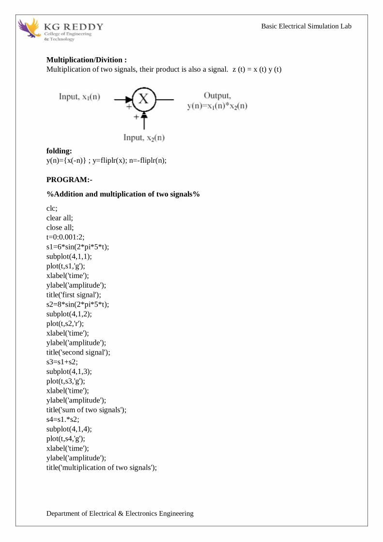
Basic Electrical Simulation Lab
Department of Electrical amp Electronics Engineering
MultiplicationDivition
Multiplication of two signals their product is also a signal z (t) = x (t) y (t)
folding
y(n)=x(-n) y=fliplr(x) n=-fliplr(n)
PROGRAM-
Addition and multiplication of two signals
clc
clear all
close all
t=000012
s1=6sin(2pi5t)
subplot(411)
plot(ts1g)
xlabel(time)
ylabel(amplitude)
title(first signal)
s2=8sin(2pi5t)
subplot(412)
plot(ts2r)
xlabel(time)
ylabel(amplitude)
title(second signal)
s3=s1+s2
subplot(413)
plot(ts3g)
xlabel(time)
ylabel(amplitude)
title(sum of two signals)
s4=s1s2
subplot(414)
plot(ts4g)
xlabel(time)
ylabel(amplitude)
title(multiplication of two signals)
Basic Electrical Simulation Lab
Department of Electrical amp Electronics Engineering
Amplitude scaling for signals
clc
clear all
close all
t=000012
s1=6sin(2pi5t)
subplot(311)
plot(ts1g)
xlabel(time)
ylabel(amplitude)
title(sinusoidal signal)
s2=3s1
subplot(312)
plot(ts2r)
xlabel(time)
ylabel(amplitude)
title(amplified signal)
s3=s13
subplot(313)
plot(ts3g)
xlabel(time)
ylabel(amplitude)
title(attenuated signal)
Time scaling for signals
clc
clear all
close all
t=000012
s1=6sin(2pi5t)
subplot(311)
plot(ts1g)
xlabel(time)
ylabel(amplitude)
title(sinusoidal signal)
t1=3t
subplot(312)
plot(t1s1r)
xlabel(time)
ylabel(amplitude)
title(compressed signal)
t2=t3
subplot(313)
plot(t2s1g)
xlabel(time)
ylabel(amplitude)
title(enlarged signal)
Basic Electrical Simulation Lab
Department of Electrical amp Electronics Engineering
Time shifting of a signal
clc
clear all
close all
t=000013
s1=6sin(2pi5t)
subplot(311)
plot(ts1g)
xlabel(time)
ylabel(amplitude)
title(sinusoidal signal)
t1=t+10
subplot(312)
plot(t1s1r)
xlabel(time)
ylabel(amplitude)
title(right shift of the signal)
t2=t-10
subplot(313)
plot(t2s1g)
xlabel(time)
ylabel(amplitude)
title(left shift of the signal)
Time folding of a signal
clc
clear all
close all
t=000012
s=sin(2pi5t)
m=length(s)
n=[-mm]
y=[0zeros(1m)s]
subplot(211)
plot(nyg)
xlabel(time)
ylabel(amplitude)
title(original signal)
y1=[fliplr(s)0zeros(1m)]
subplot(212)
plot(ny1r)
xlabel(time)
ylabel(amplitude)
title(folded signal)
Basic Electrical Simulation Lab
Department of Electrical amp Electronics Engineering
PROCEDURE-
1 Open OCTAVE
2 Open new script
3 Type the program
4 Save in current directory
5 Compile and Run the program
6 For the output see command window Figure window
OUTPUT-
RESULT-
Basic Electrical Simulation Lab
Department of Electrical amp Electronics Engineering
EXPERIMENT-4
MESH AND NODAL ANALYSIS OF ELECTRICAL CIRCUITS
AIM To Simulate the DC Circuit for determining the all node voltages and mesh currents using
NGPSPICE
APPARATUS
1 NGSPICE
2 LINUX
THEORY
NODAL ANALYSIS
In electric circuits analysis nodal analysis node-voltage analysis or the branch current
method is a method of determining the voltage (potential difference) between nodes (points
where elements or branches connect) in an electrical circuit in terms of the branch currents In
analyzing a circuit using Kirchhoffs circuit laws one can either do nodal analysis using
Kirchhoffs current law (KCL) or mesh analysis using Kirchhoffs voltage law (KVL) Nodal
analysis writes an equation at each electrical node requiring that the branch currents incident at a
node must sum to zero The branch currents are written in terms of the circuit node voltages As a
consequence each branch constitutive relation must give current as a function of voltage
an admittance representation For instance for a resistor Ibranch = Vbranch G where G (=1R) is
the admittance (conductance) of the resistor
Nodal analysis is possible when all the circuit elements branch constitutive relations have
an admittance representation Nodal analysis produces a compact set of equations for the network
which can be solved by hand if small or can be quickly solved using linear algebra by computer
Because of the compact system of equations many circuit simulation programs (eg SPICE) use
nodal analysis as a basis When elements do not have admittance representations a more general
extension of nodal analysis modified nodal analysis can be used
MESH ANALYSIS
Mesh analysis works by arbitrarily assigning mesh currents in the essential meshes (also referred
to as independent meshes) An essential mesh is a loop in the circuit that does not contain any
other loop Figure 1 labels the essential meshes with one two and three A mesh current is a
current that loops around the essential mesh and the equations are set solved in terms of them A
Basic Electrical Simulation Lab
Department of Electrical amp Electronics Engineering
mesh current may not correspond to any physically flowing current but the physical currents are
easily found from them It is usual practice to have all the mesh currents loop in the same
direction This helps prevent errors when writing out the equations The convention is to have all
the mesh currents looping in a clockwise direction
Solving for mesh currents instead of directly applying Kirchhoffs current law and Kirchhoffs
voltage law can greatly reduce the amount of calculation required This is because there are fewer
mesh currents than there are physical branch currents
CIRCUIT DIAGRAM
PROGRAM
Vs 1 0 DC 20V
Ra 1 2 5k
Rb 2 0 4k
Rc 3 0 1k
Is 3 2 DC 20mA
DC
end
OUTPUT-
RESULT-
Basic Electrical Simulation Lab
Department of Electrical amp Electronics Engineering
EXPERIMENT-5
APPLICATION OF NETWORK THEOREMS TO ELECTRICAL NETWORKS
AIM To Simulate the different network theorems to electrical networks using NGPSPICE
APPARATUS
1 NGSPICE
2 LINUX
THEORY
THEVENINrsquoS THEOREM
The Theveninrsquos Theorem states that ldquoAny two terminals linear bilateral DC network can
be replaced by an equivalent circuit consisting of a voltage source Vth in series with all equivalent
resistance Rthrdquo
(OR)
Thevenins theorem states that ldquoin any two terminal linear bilateral network having a
number of voltage current sources and resistances can be replaced by a simple equivalent circuit
consisting of a single voltage source in series with a resistance where the value of the voltage
source is equal to the open circuit voltage across the two terminals of the network and the
resistance is the equivalent resistance measured between the terminals with all energy sources
replaced by their internal resistancesrdquo
NORTONrsquoS THEOREM
Nortons theorem States that ldquoin any two terminal linear bilateral network with current
sources voltage sources and resistances can be replaced by an equivalent circuit consisting of a
current source in parallel with a resistance The value of the current source is the short circuit
current between the two terminals of the network and the resistance is the equivalent resistance
measured between the terminals of the network with all the energy sources replaced by their
internal resistancesrdquo
SUPERPOSITION THEOREM
This theorem states that ldquoThe response (voltage or current) in any branch of a bilateral
linear circuit having more than one independent source equals the algebraic sum of the responses
caused by each independent source acting alone where all the other independent sources are
replaced by their internal resistancerdquo
Basic Electrical Simulation Lab
Department of Electrical amp Electronics Engineering
i1 2kΩ
+
5000
+
minus minus
+
100i1 20kΩ
minus
1 3
2
A given response in a network regulating from a number of independent sources(including
initial condition source) may be computed by summing the response to each individual source
with all other sources made in operative( reduced to zero voltage or zero current)
This statement describes the property homogeneity in linear networks So it is the
combined properties off additivity and homogeneity off linear network It is a result of the linear
relation between current and volt in circuits having linear impedances
MAX POWER TRANSFER THEOREM
Max power will be delivered by network to the load if the impedance of network is
Complex conjugate of load impedance and vice versa
(or)
The maximum transformer states that ldquoA load will received maximum power from a
linear bilateral network when its load resistance is exactly equal to the Theveninrsquos resistance
of network measured looking back into the terminals of network
PROGRAM
THEVENINS THEORM
2mV -
Find Thevenin equivalent circuit
V10 1 0 2M V
R12 1 1A 2K
V1A 1A 2 DC 0V
E20 2 0 3 0 2E-4
F30 3 0 V1A 100
R30 3 0 20K
RL 3 0 1G
TF v(3) v10
END
NODE VOLTAGE NODE VOLTAGE NODE VOLTAGE NODE VOLTAGE
Basic Electrical Simulation Lab
Department of Electrical amp Electronics Engineering
NORTONS THEORM
PROGRAM
Vs 1 0 DC 20V
R1 1 2 18k
Rb 2 0 22k
Rc 2 3 33k
Is 3 0 RL
DC
end
MAXIMUM POWER TRANSFER THEOREM
PROGRAM
VS 1 0 DC 100
R1 1 2 10
R2 2 0 30
R3 1 3 20
R4 3 0 40
RL 2 3 RLOAD 1
MODEL RLOAD RES(R=25)
DC RES RLOAD(R) 0001 40 001
TF V(23) VS
PROBE
END
Basic Electrical Simulation Lab
Department of Electrical amp Electronics Engineering
SUPERPOSITION THEOREM
Program FOR CIRCUIT 1 FOR CIRCUIT 2
VDC 1 2 DC 10V VDC 1 2 DC 10V VDC 1 2 DC 0V
R1 1 3 100 R1 1 3 100 R1 1 3 100
R2 3 4 200 R2 3 4 200 R2 3 4 200
R3 3 6 470 R3 3 6 470 R3 3 6 470
R4 2 0 560 R4 2 0 560 R4 2 0 560
R5 4 5 100 R5 4 0 100 R5 4 5 100
VX 5 0 DC 10V VY 6 0 DC 0V VY 6 0 DC 0V
VY 6 0 DC 0V OP OP
OP END END
END
OUTPUT-
RESULT-
Basic Electrical Simulation Lab
Department of Electrical amp Electronics Engineering
EXPERIMET-6
WAVEFORM SYNTHESIS USING LAPLACE TRANSFORM
AIM To perform waveform synthesis using Laplace Transforms of a given signal
APPARATUS
1 OCTAVE
2 LINUX
THEORY
Bilateral Laplace transform
When one says the Laplace transform without qualification the unilateral or one-sided
transform is normally intended The Laplace transform can be alternatively defined as the bilateral
Laplace transform or two-sided Laplace transform by extending the limits of integration to be the
entire real axis If that is done the common unilateral transform simply becomes a special case of
the bilateral transform where the definition of the function being transformed is multiplied by the
Heaviside step function The bilateral Laplace transform is defined as follows
Inverse Laplace transform
The inverse Laplace transform is given by the following complex integral which is known by
various names (the Bromwich integral the Fourier-Mellin integral and Mellins inverse formula)
Example
Let y(t)=exp(t)
We have
The integral converges if sgt1 The functions exp(t) and 1(s-1) are partner functions
Basic Electrical Simulation Lab
Department of Electrical amp Electronics Engineering
PROGRAM-
Laplace Transform
clc
clear all
close all
syms t
x=exp(-2t)heaviside(t)
y=laplace(x)
disp(Laplace Transform of input signal)
y
z=ilaplace(y)
disp(Inverse Laplace Transform of input signal)
z
PROCEDURE-
1 Open OCTAVE
2 Open new script
3 Type the program
4 Save in current directory
5 Compile and Run the program
6 For the output see command window Figure window
OUTPUT-
RESULT-
Basic Electrical Simulation Lab
Department of Electrical amp Electronics Engineering
EXPERIMENT-7
LOCATING THE ZEROS AND POLES AND PLOTTING THE
POLE ZERO MAPS IN S-PLANE AND Z-PLANE FOR THE GIVEN
TRANSFER FUNCTION
AIM To locating the zeros and poles and plotting the pole zero maps in s-plane and z-plane
for the given transfer function
APPARATUS
1 OCTAVE
2 LINUX
THEORY
A Transfer Function is the ratio of the output of a system to the input of a system in the Laplace
domain considering its initial conditions to be zero If we have an input function of X(s) and an
output function Y(s) we define the transfer function H(s) to be
transfer function is the Laplace transform of a system‟ s impulse response
Given a continuous-time transfer function in the Laplace domain H(s) or a discrete-time one in
the Z-domain H(z) a zero is any value of s or z such that the transfer function is zero and a pole
is any value of s or z such that the transfer function is infinite
Zeros1 The value(s) for z where the numerator of the transfer function equals zero 2 The
complex frequencies that make the overall gain of the filter transfer function zero
Poles 1 The value(s) for z where the denominator of the transfer function equals zero 2 The
omplex frequencies that make the overall gain of the filter transfer function
infinite
Z-transforms
the Z-transform converts a discrete time-domain signal which is a sequence of real or complex
numbers into a complex frequency-domain representationThe Z-transform like many other
integral transforms can be defined as either a one-sided or two-sided transform
Basic Electrical Simulation Lab
Department of Electrical amp Electronics Engineering
Bilateral Z-transform
The bilateral or two-sided Z-transform of a discrete-time signal x[n] is the function X(z)
defined as
Unilateral Z-transform
Alternatively in cases where x[n] is defined only for n ge 0 the single-sided or unilateral
Z-transform is defined as
In signal processing this definition is used when the signal is causal
The roots of the equation P(z) = 0 correspond to the zeros of X(z)
The roots of the equation Q(z) = 0 correspond to the poles of X(z)
PROGRAM-
locating poles of zero on s-plane
clc
clear all
close all
num=input(enter numerator co-efficients)
den=input(enter denominator co-efficients)
h=tf(numden)
poles=roots(den)
zeros=roots(num)
sgrid
pzmap(h)
grid on
title(locating poles of zeros on s-plane)
Basic Electrical Simulation Lab
Department of Electrical amp Electronics Engineering
locating poles ampzeros on z-plane
clc
clear all
close all
num=input(enter numerator coefficient)
den=input(enter denominator coefficient)
p=roots(den)
z=roots(num)
zplane(pz)
grid
title(locating poler and zeros on s-plane)
PROCEDURE-
1 Open OCTAVE
2 Open new script
3 Type the program
4 Save in current directory
5 Compile and Run the program
6 For the output see command window Figure window
OUTPUT-
RESULT-
Basic Electrical Simulation Lab
Department of Electrical amp Electronics Engineering
EXPERIMENT-8
SIMULATION OF DC CIRCUITS
AIM To Simulate the DC network using PSPICE
APPARATUS
1 NGSPICE
2 LINUX
THEORY
Generally speaking network analysis is any structured technique used to mathematically
analyze a circuit (a ldquonetworkrdquo of interconnected components) Quite often the technician or
engineer will encounter circuits containing multiple sources of power or component
configurations which defy simplification by seriesparallel analysis techniques In those cases he
or she will be forced to use other means This chapter presents a few techniques useful in
analyzing such complex circuits
To analyse the above circuit one would first find the equivalent of R2 and R3 in parallel
then add R1 in series to arrive at a total resistance Then taking the voltage of battery B1 with
that total circuit resistance the total current could be calculated through the use of Ohmrsquos
Law (I=ER) then that current figure used to calculate voltage drops in the circuit All in all a
fairly simple procedure However the addition of just one more battery could change all of that
PROGRAM
Basic Electrical Simulation Lab
Department of Electrical amp Electronics Engineering
Vs 1 0 DC 20V
Ra 1 2 5k
Rb 2 0 4k
Rc 3 0 1k
Is 3 2 DC 20mA
DC
end
OUTPUT-
RESULT-
Basic Electrical Simulation Lab
Department of Electrical amp Electronics Engineering
EXPERIMENT-9
TRANSIENT ANALYSIS
AIM To find out the transient response by simulation of RLC circuits Using NGSPICE
APPARATUS
1 NGSPICE
2 LINUX
THEORY
The transient simulation is the calculation of a networks response on arbitrary excitations The
results are network quantities (branch currents and node voltages) as a function of time
Substantial for the transient analysis is the consideration of energy storing components ie
inductors and capacitorsThe relations between current and voltage of ideal capacitors and
inductors are given by
(61)
Or in terms of differential equations
(62)
To calculate these quantities in a computer program numerical integration methods are required
With the current-voltage relations of these components at hand it is possible to apply the modified
nodal analysis algorithm in order to calculate the networks response This means the transient
analysis attempts to find an approximation to the analytical solution at discrete time points using
numeric integration
CIRCUIT DIAGRAM
Basic Electrical Simulation Lab
Department of Electrical amp Electronics Engineering
PROGRAM
VIN1 1 0 PWL(0 0 1NS 1V 1MS 1V)
VIN2 4 0 PWL(0 0 1NS 1V 1MS 1V)
VIN3 7 0 PWL(0 0 1NS 1V 1MS 1V)
R1 1 2 2
R2 4 5 1
R3 7 8 8
L1 2 3 50UH
L2 5 6 50UH
L3 8 9 50UH
C1 3 0 10UF
C2 6 0 10UF
C3 9 0 10UF
TRAN 1US 400US
PLOT TRAN V(3) V(6) V(9)
PROBE
END
OUTPUT-
RESULT-
Basic Electrical Simulation Lab
Department of Electrical amp Electronics Engineering
EXPERIMENT-10
SIMULATION OF SINGLE PHASE DIODE BRIDGE RECTIFIERS WITH FILTER FOR
R amp RL LOAD
AIM To analyze the simulation of 1-Oslash diode bridge rectifiers with filter for R amp RL load using
NGSPICE
APPARATUS
1 NGSPICE
2 LINUX
THEORY
A bridge rectifier circuit is a common part of the electronic power supplies
Many electronic circuits require rectified DC power supply for powering the various electronic
basic components from available AC mains supply We can find this rectifier in a wide variety of
electronic AC power devices like home appliances motor controllers modulation process
welding applications etc
A Bridge rectifier is an Alternating Current (AC) to Direct Current (DC) converter that
rectifies mains AC input to DC output Bridge Rectifiers are widely used in power supplies that
provide necessary DC voltage for the electronic components or devices They can be constructed
with four or more diodes or any other controlled solid state switches Depending on the load
current requirements a proper bridge rectifier is selected Componentsrsquo ratings and specifications
breakdown voltage temperature ranges transient current rating forward current rating mounting
requirements and other considerations are taken into account while selecting a rectifier power
supply for an appropriate electronic circuitrsquos application
Bride rectifiers are classified into several types based on these factors type of supply
controlling capability bride circuitrsquos configurations etc Bridge rectifiers are mainly classified
into single and three phase rectifiers Both these types are further classified into uncontrolled half
controlled and full controlled rectifiers
Basic Electrical Simulation Lab
Department of Electrical amp Electronics Engineering
Program
VS 1 0 SIN(0 1697V 60HZ)
DF 5 4 DMOD
R1 4 7 10
L1 7 8 20MH
C1 4 6 793UF
RX 6 5 01
VX 8 5 DC 10V
VY 2 1 DC 0V
D1 2 4 DMOD
D2 5 3 DMOD
D3 3 4 DMOD
D4 5 2 DMOD
MODEL DMOD D( IS=22E-15 BV=1800 TT=0)
TRAN 10US 100MS 166MS
PROBE
FOUR 120HZ I(VX)
END
OUTPUT-
RESULT-
Basic Electrical Simulation Lab
Department of Electrical amp Electronics Engineering
EXPERIMENT-11
SIMULATION OF THREE PHASE DIODE BRIDGE RECTIFIERS WITH R RL LOAD
AIM To analyze the simulation of 3-Oslash diode bridge rectifiers with filter for R amp RL load using
NGSPICE
APPARATUS
1 NGSPICE
2 LINUX
THEORY
Three phase half controlled bridge converters amp fully controlled bridge converters are used
extensively in industrial applications up to about 15kW of output power The Three phase
controlled rectifiers provide a maximum dc output of
vdc(max)=2vm prod
The output ripple frequency is equal to the twice the ac supply frequency The single phase
full wave controlled rectifiers provide two output pulses during every input supply cycle
and hence are referred to as two pulse converters
Three phase converters are 3-phase controlled rectifiers which are used to convert ac input
power supply into dc output power across the load
Features of 3-phase controlled rectifiers are
Operate from 3 phase ac supply voltage
They provide higher dc output voltage and higher dc output power
Higher output voltage ripple frequency
Filtering requirements are simplified for smoothing out load voltage and load
current
Three phase controlled rectifiers are extensively used in high power variable speed
industrial dc drives
Basic Electrical Simulation Lab
Department of Electrical amp Electronics Engineering
Program
VAN 1 0 SIN(0V 200V 50HZ 0 0 0)
VBN 2 0 SIN(0V 200V 50HZ 0 0 -120)
VCN 3 0 SIN(0V 200V 50HZ 0 0 -240)
R 7 9 20
L 9 10 55MH
VX 10 8 DC 0V
VY 1 4 DC 0V
D1 4 7 DMOD
D2 8 2 DMOD
D3 3 7 DMOD
D4 8 4 DMOD
D5 2 7 DMOD
D6 8 3 DMOD
MODEL DMOD D(IS=22E-15 BV=1800V TT=0)
TRAN 5US 50MS 2166MS
PROBE
END
OUTPUT-
RESULT-
Basic Electrical Simulation Lab
Department of Electrical amp Electronics Engineering
EXPERIMENT-12
DESIGN OF LOW PASS AND HIGH PASS FILTERS
AIM To analyze the simulation of 3-Oslash diode bridge rectifiers with filter for R amp RL load using
NGSPICE
APPARATUS
1 OCTAVE
2 LINUX
THEORY
A filter is a circuit that has designed to pass a specified band of frequencies while attenuating all
signals outside this band Active filters employ transistors or op-amps plus resistors inductors
and capacitors There are four types of filters low-pass high-pass band-pass and band-
elimination (also referred to as band-reject or notch) filters Figure 71 illustrates frequency-
response plot for the four types of filters A low-pass filter is a circuit that has a constant output
voltage from dc up to a cutoff frequency fc As the frequency increases above fc the output
voltage is attenuated (decreases) Figure 71(a) is a plot of magnitude of the output voltage of a
low-pass filter versus frequency The range of frequencies that are transmitted is known as the
pass-band The range of frequencies that are attenuated is known as the stop-band The cutoff
frequency fc is also called the 0707 frequency the 3-dB frequency the corner frequency or the
break frequency High-pass filters attenuate the output voltage for all frequencies below the cutoff
frequency fc Above fc the magnitude of the output voltage is constant Figure 71(b) is the plot
for ideal and practical high-pass filters Band-pass filters pass only a band of frequencies while
attenuating all frequencies outside the band Band-elimination filters perform in an exactly
opposite way that is band-elimination filters reject a specified band of frequencies while passing
all frequencies outside the band Typical frequency-response plots for band-pass and band-
elimination filters are shown in Figure 71(c) and (d) In many filter applications it is necessary
for the closed-loop gain to be as close to 1 as possible within the pass band The Butterworth filter
is best suited for this type of application The Butterworth filter is also called a maximally flat or
flat-flat filter and all filter in this experiment will be of the Butterworth type Figure 72 shows
the ideal and the practical frequency response for three types of Butterworth filters As the roll-
offs become steeper they approach the ideal filter more closely
Basic Electrical Simulation Lab
Department of Electrical amp Electronics Engineering
PROGRAM
LOW PASS FILTER
N = 100 FIR filter order
Fp = 20e3 20 kHz passband-edge frequency
Fs = 96e3 96 kHz sampling frequency
Rp = 000057565 Corresponds to 001 dB peak-to-peak ripple
Rst = 1e-4 Corresponds to 80 dB stopband attenuation
eqnum = firceqrip(NFp(Fs2)[Rp Rst]passedge) eqnum = vec of coeffs
fvtool(eqnumFsFsColorWhite) Visualize filter
HIGH PASS FILTER
Fstop = 350
Fpass = 400
Astop = 65
Apass = 05
Fs = 1e3
d = designfilt(highpassfirStopbandFrequencyFstop
PassbandFrequencyFpassStopbandAttenuationAstop
PassbandRippleApassSampleRateFsDesignMethodequiripple)
fvtool(d)
OUTPUT-
RESULT-
Basic Electrical Simulation Lab
Department of Electrical amp Electronics Engineering
EXPERIMENT-13
FINDING THE EVEN AND ODD PARTS OF SIGNAL SEQUENCE AND REAL AND
IMAGINARY PARTS OF SIGNAL
AIM
program for finding even and odd parts of sequences Using OCTAVE Softwareamp
program for finding real and imaginary parts of sequences Using OCTAVE Software
APPARATUS
1 OCTAVE
2 LINUX
THEORY
Even and Odd Signal
One of characteristics of signal is symmetry that may be useful for signal analysis Even signals
are symmetric around vertical axis and Odd signals are symmetric about origin
Even Signal A signal is referred to as an even if it is identical to its time-reversed counterparts
x(t) = x(-t)
Odd Signal A signal is odd if x(t) = -x(-t)
An odd signal must be 0 at t=0 in other words odd signal passes the origin
Using the definition of even and odd signal any signal may be decomposed into a sum of its even
part xe(t) and its odd part xo(t) as follows
x(t)=xe(t)+xo(t)
x(t)=12x(t)+x(-t) +12x(t)-x(-t)
where
xe(t)=12x(t)+x(-t) ampxo(t)=12x(t)-x(-t)
It is an important fact because it is relative concept of Fourier series In Fourier series aperiodic
signal can be broken into a sum of sine and cosine signals Notice that sine function is odd signal
and cosine function is even signal
ENERGY AND POWER SIGNAL
A signal can be categorized into energy signal or power
signal An energy signal has a finite energy 0 lt E lt 1049279 In other words energy signals have
values only in the limited time duration For example a signal having only one square pulse is
energy signal A signal that decays exponentially has finite energy so it is also an energy signal
The power of an energy signal is 0 because of dividing finite energy by infinite time (or length)
If x(t) is a real-valued signal with Fourier transform X(f) and u(f) is the Heaviside step function
Basic Electrical Simulation Lab
Department of Electrical amp Electronics Engineering
then the function
contains only the non-negative frequency components of X(f) And the operation is reversible due
to the Hermitian property of X(f)
X(f) denotes the complex conjugate of X(f)
The inverse Fourier transform of Xa(f) is the analytic signal
where x^(t) is the Hilbert transform of x(t) and J is the imaginary unit
Basic Electrical Simulation Lab
Department of Electrical amp Electronics Engineering
PROGRAM-
Evenoddrealimaginary parts of a sequences
clc
clear all
close all
h=input(enter noof samples)
m=(h-1)2
n=-mm
x=input(enter sample values)
subplot(411)
stem(nxg)
xlabel(time)
ylabel(amplitude)
title(original sequence)
xmir=fliplr(x)
subplot(412)
stem(nxmirr)
xlabel(time)
ylabel(amplitude)
title(folded sequence)
even part of sequence
xeven=(x+xmir)2
subplot(413)
stem(nxevenr)
xlabel(time)
ylabel(amplitude)
title(even part of sequence)
odd part of sequence
xodd=(x-xmir)2
subplot(414)
stem(nxoddg)
xlabel(time)
ylabel(amplitude)
title(odd part of sequence)
Basic Electrical Simulation Lab
Department of Electrical amp Electronics Engineering
RealampImaginary parts of a sequences
clc
clear all
close all
y=input(enter complex numbers)
yreal=real(y)
disp(real values of y)
yreal
yimag=imag(y)
disp(imaginary values of y)
yimag
PROCEDURE-
1 Open OCTAVE
2 Open new script
3 Type the program
4 Save in current directory
5 Compile and Run the program
6 For the output see command window Figure window
OUTPUT-
RESULT-
Basic Electrical Simulation Lab
Department of Electrical amp Electronics Engineering
EXPERIMENT-14
FINDING THE FOURIER TRANSFORM OF A GIVEN SIGNAL AND PLOTTING ITS
MAGNITUDE AND PHASE SPECTRUM
AIM
Program for finding the fourier transform of a given signal Using OCTAVE Software amp Plotting
Its Magnitude And Phase Spectrum Using OCTAVE Software
APPARATUS
1 OCTAVE
2 LINUX
THEORY
The Fourier transform (FT) decomposes a function of time (a signal) into the
frequencies that make it up in a way similar to how a musical chord can be expressed as the
frequencies (or pitches) of its constituent notes The Fourier transform of a function of time itself
is a complex-valued function of frequency whose absolute value represents the amount of that
frequency present in the original function and whose complex argument is the phase offset of the
basic sinusoid in that frequency The Fourier transform is called the frequency domain
representation of the original signal The term Fourier transform refers to both the frequency
domain representation and the mathematical operation that associates the frequency domain
representation to a function of time The Fourier transform is not limited to functions of time but
in order to have a unified language the domain of the original function is commonly referred to as
the time domain For many functions of practical interest one can define an operation that
reverses this the inverse Fourier transformation also called Fourier synthesis of a frequency
domain representation combines the contributions of all the different frequencies to recover the
original function of time
Linear operations performed in one domain (time or frequency) have corresponding
operations in the other domain which are sometimes easier to perform The operation
of differentiation in the time domain corresponds to multiplication by the frequency[remark 1] so
some differential equations are easier to analyze in the frequency domain Also convolution in the
time domain corresponds to ordinary multiplication in the frequency domain Concretely this
means that any linear time-invariant system such as a filter applied to a signal can be expressed
relatively simply as an operation on frequencies After performing the desired operations
transformation of the result can be made back to the time domain Harmonic analysis is the
systematic study of the relationship between the frequency and time domains including the kinds
Basic Electrical Simulation Lab
Department of Electrical amp Electronics Engineering
of functions or operations that are simpler in one or the other and has deep connections to many
areas of modern mathematics
PROGRAM
Fs = 1000 Sampling frequency
T = 1Fs Sampling period
L = 1500 Length of signal
t = (0L-1)T Time vector
S = 07sin(2pi50t) + sin(2pi120t)
X = S + 2randn(size(t))
plot(1000t(150)X(150))
title(Signal Corrupted with Zero-Mean Random Noise)
xlabel(t (milliseconds))
ylabel(X(t))
Y = fft(X)
P2 = abs(YL)
P1 = P2(1L2+1)
P1(2end-1) = 2P1(2end-1)
f = Fs(0(L2))L
plot(fP1)
title(Single-Sided Amplitude Spectrum of X(t))
xlabel(f (Hz))
ylabel(|P1(f)|)
Y = fft(S)
P2 = abs(YL)
P1 = P2(1L2+1)
P1(2end-1) = 2P1(2end-1)
plot(fP1)
title(Single-Sided Amplitude Spectrum of S(t))
xlabel(f (Hz))
ylabel(|P1(f)|)
OUTPUT-
RESULT-
Basic Electrical Simulation Lab
Department of Electrical amp Electronics Engineering
Amplitude scaling for signals
clc
clear all
close all
t=000012
s1=6sin(2pi5t)
subplot(311)
plot(ts1g)
xlabel(time)
ylabel(amplitude)
title(sinusoidal signal)
s2=3s1
subplot(312)
plot(ts2r)
xlabel(time)
ylabel(amplitude)
title(amplified signal)
s3=s13
subplot(313)
plot(ts3g)
xlabel(time)
ylabel(amplitude)
title(attenuated signal)
Time scaling for signals
clc
clear all
close all
t=000012
s1=6sin(2pi5t)
subplot(311)
plot(ts1g)
xlabel(time)
ylabel(amplitude)
title(sinusoidal signal)
t1=3t
subplot(312)
plot(t1s1r)
xlabel(time)
ylabel(amplitude)
title(compressed signal)
t2=t3
subplot(313)
plot(t2s1g)
xlabel(time)
ylabel(amplitude)
title(enlarged signal)
Basic Electrical Simulation Lab
Department of Electrical amp Electronics Engineering
Time shifting of a signal
clc
clear all
close all
t=000013
s1=6sin(2pi5t)
subplot(311)
plot(ts1g)
xlabel(time)
ylabel(amplitude)
title(sinusoidal signal)
t1=t+10
subplot(312)
plot(t1s1r)
xlabel(time)
ylabel(amplitude)
title(right shift of the signal)
t2=t-10
subplot(313)
plot(t2s1g)
xlabel(time)
ylabel(amplitude)
title(left shift of the signal)
Time folding of a signal
clc
clear all
close all
t=000012
s=sin(2pi5t)
m=length(s)
n=[-mm]
y=[0zeros(1m)s]
subplot(211)
plot(nyg)
xlabel(time)
ylabel(amplitude)
title(original signal)
y1=[fliplr(s)0zeros(1m)]
subplot(212)
plot(ny1r)
xlabel(time)
ylabel(amplitude)
title(folded signal)
Basic Electrical Simulation Lab
Department of Electrical amp Electronics Engineering
PROCEDURE-
1 Open OCTAVE
2 Open new script
3 Type the program
4 Save in current directory
5 Compile and Run the program
6 For the output see command window Figure window
OUTPUT-
RESULT-
Basic Electrical Simulation Lab
Department of Electrical amp Electronics Engineering
EXPERIMENT-4
MESH AND NODAL ANALYSIS OF ELECTRICAL CIRCUITS
AIM To Simulate the DC Circuit for determining the all node voltages and mesh currents using
NGPSPICE
APPARATUS
1 NGSPICE
2 LINUX
THEORY
NODAL ANALYSIS
In electric circuits analysis nodal analysis node-voltage analysis or the branch current
method is a method of determining the voltage (potential difference) between nodes (points
where elements or branches connect) in an electrical circuit in terms of the branch currents In
analyzing a circuit using Kirchhoffs circuit laws one can either do nodal analysis using
Kirchhoffs current law (KCL) or mesh analysis using Kirchhoffs voltage law (KVL) Nodal
analysis writes an equation at each electrical node requiring that the branch currents incident at a
node must sum to zero The branch currents are written in terms of the circuit node voltages As a
consequence each branch constitutive relation must give current as a function of voltage
an admittance representation For instance for a resistor Ibranch = Vbranch G where G (=1R) is
the admittance (conductance) of the resistor
Nodal analysis is possible when all the circuit elements branch constitutive relations have
an admittance representation Nodal analysis produces a compact set of equations for the network
which can be solved by hand if small or can be quickly solved using linear algebra by computer
Because of the compact system of equations many circuit simulation programs (eg SPICE) use
nodal analysis as a basis When elements do not have admittance representations a more general
extension of nodal analysis modified nodal analysis can be used
MESH ANALYSIS
Mesh analysis works by arbitrarily assigning mesh currents in the essential meshes (also referred
to as independent meshes) An essential mesh is a loop in the circuit that does not contain any
other loop Figure 1 labels the essential meshes with one two and three A mesh current is a
current that loops around the essential mesh and the equations are set solved in terms of them A
Basic Electrical Simulation Lab
Department of Electrical amp Electronics Engineering
mesh current may not correspond to any physically flowing current but the physical currents are
easily found from them It is usual practice to have all the mesh currents loop in the same
direction This helps prevent errors when writing out the equations The convention is to have all
the mesh currents looping in a clockwise direction
Solving for mesh currents instead of directly applying Kirchhoffs current law and Kirchhoffs
voltage law can greatly reduce the amount of calculation required This is because there are fewer
mesh currents than there are physical branch currents
CIRCUIT DIAGRAM
PROGRAM
Vs 1 0 DC 20V
Ra 1 2 5k
Rb 2 0 4k
Rc 3 0 1k
Is 3 2 DC 20mA
DC
end
OUTPUT-
RESULT-
Basic Electrical Simulation Lab
Department of Electrical amp Electronics Engineering
EXPERIMENT-5
APPLICATION OF NETWORK THEOREMS TO ELECTRICAL NETWORKS
AIM To Simulate the different network theorems to electrical networks using NGPSPICE
APPARATUS
1 NGSPICE
2 LINUX
THEORY
THEVENINrsquoS THEOREM
The Theveninrsquos Theorem states that ldquoAny two terminals linear bilateral DC network can
be replaced by an equivalent circuit consisting of a voltage source Vth in series with all equivalent
resistance Rthrdquo
(OR)
Thevenins theorem states that ldquoin any two terminal linear bilateral network having a
number of voltage current sources and resistances can be replaced by a simple equivalent circuit
consisting of a single voltage source in series with a resistance where the value of the voltage
source is equal to the open circuit voltage across the two terminals of the network and the
resistance is the equivalent resistance measured between the terminals with all energy sources
replaced by their internal resistancesrdquo
NORTONrsquoS THEOREM
Nortons theorem States that ldquoin any two terminal linear bilateral network with current
sources voltage sources and resistances can be replaced by an equivalent circuit consisting of a
current source in parallel with a resistance The value of the current source is the short circuit
current between the two terminals of the network and the resistance is the equivalent resistance
measured between the terminals of the network with all the energy sources replaced by their
internal resistancesrdquo
SUPERPOSITION THEOREM
This theorem states that ldquoThe response (voltage or current) in any branch of a bilateral
linear circuit having more than one independent source equals the algebraic sum of the responses
caused by each independent source acting alone where all the other independent sources are
replaced by their internal resistancerdquo
Basic Electrical Simulation Lab
Department of Electrical amp Electronics Engineering
i1 2kΩ
+
5000
+
minus minus
+
100i1 20kΩ
minus
1 3
2
A given response in a network regulating from a number of independent sources(including
initial condition source) may be computed by summing the response to each individual source
with all other sources made in operative( reduced to zero voltage or zero current)
This statement describes the property homogeneity in linear networks So it is the
combined properties off additivity and homogeneity off linear network It is a result of the linear
relation between current and volt in circuits having linear impedances
MAX POWER TRANSFER THEOREM
Max power will be delivered by network to the load if the impedance of network is
Complex conjugate of load impedance and vice versa
(or)
The maximum transformer states that ldquoA load will received maximum power from a
linear bilateral network when its load resistance is exactly equal to the Theveninrsquos resistance
of network measured looking back into the terminals of network
PROGRAM
THEVENINS THEORM
2mV -
Find Thevenin equivalent circuit
V10 1 0 2M V
R12 1 1A 2K
V1A 1A 2 DC 0V
E20 2 0 3 0 2E-4
F30 3 0 V1A 100
R30 3 0 20K
RL 3 0 1G
TF v(3) v10
END
NODE VOLTAGE NODE VOLTAGE NODE VOLTAGE NODE VOLTAGE
Basic Electrical Simulation Lab
Department of Electrical amp Electronics Engineering
NORTONS THEORM
PROGRAM
Vs 1 0 DC 20V
R1 1 2 18k
Rb 2 0 22k
Rc 2 3 33k
Is 3 0 RL
DC
end
MAXIMUM POWER TRANSFER THEOREM
PROGRAM
VS 1 0 DC 100
R1 1 2 10
R2 2 0 30
R3 1 3 20
R4 3 0 40
RL 2 3 RLOAD 1
MODEL RLOAD RES(R=25)
DC RES RLOAD(R) 0001 40 001
TF V(23) VS
PROBE
END
Basic Electrical Simulation Lab
Department of Electrical amp Electronics Engineering
SUPERPOSITION THEOREM
Program FOR CIRCUIT 1 FOR CIRCUIT 2
VDC 1 2 DC 10V VDC 1 2 DC 10V VDC 1 2 DC 0V
R1 1 3 100 R1 1 3 100 R1 1 3 100
R2 3 4 200 R2 3 4 200 R2 3 4 200
R3 3 6 470 R3 3 6 470 R3 3 6 470
R4 2 0 560 R4 2 0 560 R4 2 0 560
R5 4 5 100 R5 4 0 100 R5 4 5 100
VX 5 0 DC 10V VY 6 0 DC 0V VY 6 0 DC 0V
VY 6 0 DC 0V OP OP
OP END END
END
OUTPUT-
RESULT-
Basic Electrical Simulation Lab
Department of Electrical amp Electronics Engineering
EXPERIMET-6
WAVEFORM SYNTHESIS USING LAPLACE TRANSFORM
AIM To perform waveform synthesis using Laplace Transforms of a given signal
APPARATUS
1 OCTAVE
2 LINUX
THEORY
Bilateral Laplace transform
When one says the Laplace transform without qualification the unilateral or one-sided
transform is normally intended The Laplace transform can be alternatively defined as the bilateral
Laplace transform or two-sided Laplace transform by extending the limits of integration to be the
entire real axis If that is done the common unilateral transform simply becomes a special case of
the bilateral transform where the definition of the function being transformed is multiplied by the
Heaviside step function The bilateral Laplace transform is defined as follows
Inverse Laplace transform
The inverse Laplace transform is given by the following complex integral which is known by
various names (the Bromwich integral the Fourier-Mellin integral and Mellins inverse formula)
Example
Let y(t)=exp(t)
We have
The integral converges if sgt1 The functions exp(t) and 1(s-1) are partner functions
Basic Electrical Simulation Lab
Department of Electrical amp Electronics Engineering
PROGRAM-
Laplace Transform
clc
clear all
close all
syms t
x=exp(-2t)heaviside(t)
y=laplace(x)
disp(Laplace Transform of input signal)
y
z=ilaplace(y)
disp(Inverse Laplace Transform of input signal)
z
PROCEDURE-
1 Open OCTAVE
2 Open new script
3 Type the program
4 Save in current directory
5 Compile and Run the program
6 For the output see command window Figure window
OUTPUT-
RESULT-
Basic Electrical Simulation Lab
Department of Electrical amp Electronics Engineering
EXPERIMENT-7
LOCATING THE ZEROS AND POLES AND PLOTTING THE
POLE ZERO MAPS IN S-PLANE AND Z-PLANE FOR THE GIVEN
TRANSFER FUNCTION
AIM To locating the zeros and poles and plotting the pole zero maps in s-plane and z-plane
for the given transfer function
APPARATUS
1 OCTAVE
2 LINUX
THEORY
A Transfer Function is the ratio of the output of a system to the input of a system in the Laplace
domain considering its initial conditions to be zero If we have an input function of X(s) and an
output function Y(s) we define the transfer function H(s) to be
transfer function is the Laplace transform of a system‟ s impulse response
Given a continuous-time transfer function in the Laplace domain H(s) or a discrete-time one in
the Z-domain H(z) a zero is any value of s or z such that the transfer function is zero and a pole
is any value of s or z such that the transfer function is infinite
Zeros1 The value(s) for z where the numerator of the transfer function equals zero 2 The
complex frequencies that make the overall gain of the filter transfer function zero
Poles 1 The value(s) for z where the denominator of the transfer function equals zero 2 The
omplex frequencies that make the overall gain of the filter transfer function
infinite
Z-transforms
the Z-transform converts a discrete time-domain signal which is a sequence of real or complex
numbers into a complex frequency-domain representationThe Z-transform like many other
integral transforms can be defined as either a one-sided or two-sided transform
Basic Electrical Simulation Lab
Department of Electrical amp Electronics Engineering
Bilateral Z-transform
The bilateral or two-sided Z-transform of a discrete-time signal x[n] is the function X(z)
defined as
Unilateral Z-transform
Alternatively in cases where x[n] is defined only for n ge 0 the single-sided or unilateral
Z-transform is defined as
In signal processing this definition is used when the signal is causal
The roots of the equation P(z) = 0 correspond to the zeros of X(z)
The roots of the equation Q(z) = 0 correspond to the poles of X(z)
PROGRAM-
locating poles of zero on s-plane
clc
clear all
close all
num=input(enter numerator co-efficients)
den=input(enter denominator co-efficients)
h=tf(numden)
poles=roots(den)
zeros=roots(num)
sgrid
pzmap(h)
grid on
title(locating poles of zeros on s-plane)
Basic Electrical Simulation Lab
Department of Electrical amp Electronics Engineering
locating poles ampzeros on z-plane
clc
clear all
close all
num=input(enter numerator coefficient)
den=input(enter denominator coefficient)
p=roots(den)
z=roots(num)
zplane(pz)
grid
title(locating poler and zeros on s-plane)
PROCEDURE-
1 Open OCTAVE
2 Open new script
3 Type the program
4 Save in current directory
5 Compile and Run the program
6 For the output see command window Figure window
OUTPUT-
RESULT-
Basic Electrical Simulation Lab
Department of Electrical amp Electronics Engineering
EXPERIMENT-8
SIMULATION OF DC CIRCUITS
AIM To Simulate the DC network using PSPICE
APPARATUS
1 NGSPICE
2 LINUX
THEORY
Generally speaking network analysis is any structured technique used to mathematically
analyze a circuit (a ldquonetworkrdquo of interconnected components) Quite often the technician or
engineer will encounter circuits containing multiple sources of power or component
configurations which defy simplification by seriesparallel analysis techniques In those cases he
or she will be forced to use other means This chapter presents a few techniques useful in
analyzing such complex circuits
To analyse the above circuit one would first find the equivalent of R2 and R3 in parallel
then add R1 in series to arrive at a total resistance Then taking the voltage of battery B1 with
that total circuit resistance the total current could be calculated through the use of Ohmrsquos
Law (I=ER) then that current figure used to calculate voltage drops in the circuit All in all a
fairly simple procedure However the addition of just one more battery could change all of that
PROGRAM
Basic Electrical Simulation Lab
Department of Electrical amp Electronics Engineering
Vs 1 0 DC 20V
Ra 1 2 5k
Rb 2 0 4k
Rc 3 0 1k
Is 3 2 DC 20mA
DC
end
OUTPUT-
RESULT-
Basic Electrical Simulation Lab
Department of Electrical amp Electronics Engineering
EXPERIMENT-9
TRANSIENT ANALYSIS
AIM To find out the transient response by simulation of RLC circuits Using NGSPICE
APPARATUS
1 NGSPICE
2 LINUX
THEORY
The transient simulation is the calculation of a networks response on arbitrary excitations The
results are network quantities (branch currents and node voltages) as a function of time
Substantial for the transient analysis is the consideration of energy storing components ie
inductors and capacitorsThe relations between current and voltage of ideal capacitors and
inductors are given by
(61)
Or in terms of differential equations
(62)
To calculate these quantities in a computer program numerical integration methods are required
With the current-voltage relations of these components at hand it is possible to apply the modified
nodal analysis algorithm in order to calculate the networks response This means the transient
analysis attempts to find an approximation to the analytical solution at discrete time points using
numeric integration
CIRCUIT DIAGRAM
Basic Electrical Simulation Lab
Department of Electrical amp Electronics Engineering
PROGRAM
VIN1 1 0 PWL(0 0 1NS 1V 1MS 1V)
VIN2 4 0 PWL(0 0 1NS 1V 1MS 1V)
VIN3 7 0 PWL(0 0 1NS 1V 1MS 1V)
R1 1 2 2
R2 4 5 1
R3 7 8 8
L1 2 3 50UH
L2 5 6 50UH
L3 8 9 50UH
C1 3 0 10UF
C2 6 0 10UF
C3 9 0 10UF
TRAN 1US 400US
PLOT TRAN V(3) V(6) V(9)
PROBE
END
OUTPUT-
RESULT-
Basic Electrical Simulation Lab
Department of Electrical amp Electronics Engineering
EXPERIMENT-10
SIMULATION OF SINGLE PHASE DIODE BRIDGE RECTIFIERS WITH FILTER FOR
R amp RL LOAD
AIM To analyze the simulation of 1-Oslash diode bridge rectifiers with filter for R amp RL load using
NGSPICE
APPARATUS
1 NGSPICE
2 LINUX
THEORY
A bridge rectifier circuit is a common part of the electronic power supplies
Many electronic circuits require rectified DC power supply for powering the various electronic
basic components from available AC mains supply We can find this rectifier in a wide variety of
electronic AC power devices like home appliances motor controllers modulation process
welding applications etc
A Bridge rectifier is an Alternating Current (AC) to Direct Current (DC) converter that
rectifies mains AC input to DC output Bridge Rectifiers are widely used in power supplies that
provide necessary DC voltage for the electronic components or devices They can be constructed
with four or more diodes or any other controlled solid state switches Depending on the load
current requirements a proper bridge rectifier is selected Componentsrsquo ratings and specifications
breakdown voltage temperature ranges transient current rating forward current rating mounting
requirements and other considerations are taken into account while selecting a rectifier power
supply for an appropriate electronic circuitrsquos application
Bride rectifiers are classified into several types based on these factors type of supply
controlling capability bride circuitrsquos configurations etc Bridge rectifiers are mainly classified
into single and three phase rectifiers Both these types are further classified into uncontrolled half
controlled and full controlled rectifiers
Basic Electrical Simulation Lab
Department of Electrical amp Electronics Engineering
Program
VS 1 0 SIN(0 1697V 60HZ)
DF 5 4 DMOD
R1 4 7 10
L1 7 8 20MH
C1 4 6 793UF
RX 6 5 01
VX 8 5 DC 10V
VY 2 1 DC 0V
D1 2 4 DMOD
D2 5 3 DMOD
D3 3 4 DMOD
D4 5 2 DMOD
MODEL DMOD D( IS=22E-15 BV=1800 TT=0)
TRAN 10US 100MS 166MS
PROBE
FOUR 120HZ I(VX)
END
OUTPUT-
RESULT-
Basic Electrical Simulation Lab
Department of Electrical amp Electronics Engineering
EXPERIMENT-11
SIMULATION OF THREE PHASE DIODE BRIDGE RECTIFIERS WITH R RL LOAD
AIM To analyze the simulation of 3-Oslash diode bridge rectifiers with filter for R amp RL load using
NGSPICE
APPARATUS
1 NGSPICE
2 LINUX
THEORY
Three phase half controlled bridge converters amp fully controlled bridge converters are used
extensively in industrial applications up to about 15kW of output power The Three phase
controlled rectifiers provide a maximum dc output of
vdc(max)=2vm prod
The output ripple frequency is equal to the twice the ac supply frequency The single phase
full wave controlled rectifiers provide two output pulses during every input supply cycle
and hence are referred to as two pulse converters
Three phase converters are 3-phase controlled rectifiers which are used to convert ac input
power supply into dc output power across the load
Features of 3-phase controlled rectifiers are
Operate from 3 phase ac supply voltage
They provide higher dc output voltage and higher dc output power
Higher output voltage ripple frequency
Filtering requirements are simplified for smoothing out load voltage and load
current
Three phase controlled rectifiers are extensively used in high power variable speed
industrial dc drives
Basic Electrical Simulation Lab
Department of Electrical amp Electronics Engineering
Program
VAN 1 0 SIN(0V 200V 50HZ 0 0 0)
VBN 2 0 SIN(0V 200V 50HZ 0 0 -120)
VCN 3 0 SIN(0V 200V 50HZ 0 0 -240)
R 7 9 20
L 9 10 55MH
VX 10 8 DC 0V
VY 1 4 DC 0V
D1 4 7 DMOD
D2 8 2 DMOD
D3 3 7 DMOD
D4 8 4 DMOD
D5 2 7 DMOD
D6 8 3 DMOD
MODEL DMOD D(IS=22E-15 BV=1800V TT=0)
TRAN 5US 50MS 2166MS
PROBE
END
OUTPUT-
RESULT-
Basic Electrical Simulation Lab
Department of Electrical amp Electronics Engineering
EXPERIMENT-12
DESIGN OF LOW PASS AND HIGH PASS FILTERS
AIM To analyze the simulation of 3-Oslash diode bridge rectifiers with filter for R amp RL load using
NGSPICE
APPARATUS
1 OCTAVE
2 LINUX
THEORY
A filter is a circuit that has designed to pass a specified band of frequencies while attenuating all
signals outside this band Active filters employ transistors or op-amps plus resistors inductors
and capacitors There are four types of filters low-pass high-pass band-pass and band-
elimination (also referred to as band-reject or notch) filters Figure 71 illustrates frequency-
response plot for the four types of filters A low-pass filter is a circuit that has a constant output
voltage from dc up to a cutoff frequency fc As the frequency increases above fc the output
voltage is attenuated (decreases) Figure 71(a) is a plot of magnitude of the output voltage of a
low-pass filter versus frequency The range of frequencies that are transmitted is known as the
pass-band The range of frequencies that are attenuated is known as the stop-band The cutoff
frequency fc is also called the 0707 frequency the 3-dB frequency the corner frequency or the
break frequency High-pass filters attenuate the output voltage for all frequencies below the cutoff
frequency fc Above fc the magnitude of the output voltage is constant Figure 71(b) is the plot
for ideal and practical high-pass filters Band-pass filters pass only a band of frequencies while
attenuating all frequencies outside the band Band-elimination filters perform in an exactly
opposite way that is band-elimination filters reject a specified band of frequencies while passing
all frequencies outside the band Typical frequency-response plots for band-pass and band-
elimination filters are shown in Figure 71(c) and (d) In many filter applications it is necessary
for the closed-loop gain to be as close to 1 as possible within the pass band The Butterworth filter
is best suited for this type of application The Butterworth filter is also called a maximally flat or
flat-flat filter and all filter in this experiment will be of the Butterworth type Figure 72 shows
the ideal and the practical frequency response for three types of Butterworth filters As the roll-
offs become steeper they approach the ideal filter more closely
Basic Electrical Simulation Lab
Department of Electrical amp Electronics Engineering
PROGRAM
LOW PASS FILTER
N = 100 FIR filter order
Fp = 20e3 20 kHz passband-edge frequency
Fs = 96e3 96 kHz sampling frequency
Rp = 000057565 Corresponds to 001 dB peak-to-peak ripple
Rst = 1e-4 Corresponds to 80 dB stopband attenuation
eqnum = firceqrip(NFp(Fs2)[Rp Rst]passedge) eqnum = vec of coeffs
fvtool(eqnumFsFsColorWhite) Visualize filter
HIGH PASS FILTER
Fstop = 350
Fpass = 400
Astop = 65
Apass = 05
Fs = 1e3
d = designfilt(highpassfirStopbandFrequencyFstop
PassbandFrequencyFpassStopbandAttenuationAstop
PassbandRippleApassSampleRateFsDesignMethodequiripple)
fvtool(d)
OUTPUT-
RESULT-
Basic Electrical Simulation Lab
Department of Electrical amp Electronics Engineering
EXPERIMENT-13
FINDING THE EVEN AND ODD PARTS OF SIGNAL SEQUENCE AND REAL AND
IMAGINARY PARTS OF SIGNAL
AIM
program for finding even and odd parts of sequences Using OCTAVE Softwareamp
program for finding real and imaginary parts of sequences Using OCTAVE Software
APPARATUS
1 OCTAVE
2 LINUX
THEORY
Even and Odd Signal
One of characteristics of signal is symmetry that may be useful for signal analysis Even signals
are symmetric around vertical axis and Odd signals are symmetric about origin
Even Signal A signal is referred to as an even if it is identical to its time-reversed counterparts
x(t) = x(-t)
Odd Signal A signal is odd if x(t) = -x(-t)
An odd signal must be 0 at t=0 in other words odd signal passes the origin
Using the definition of even and odd signal any signal may be decomposed into a sum of its even
part xe(t) and its odd part xo(t) as follows
x(t)=xe(t)+xo(t)
x(t)=12x(t)+x(-t) +12x(t)-x(-t)
where
xe(t)=12x(t)+x(-t) ampxo(t)=12x(t)-x(-t)
It is an important fact because it is relative concept of Fourier series In Fourier series aperiodic
signal can be broken into a sum of sine and cosine signals Notice that sine function is odd signal
and cosine function is even signal
ENERGY AND POWER SIGNAL
A signal can be categorized into energy signal or power
signal An energy signal has a finite energy 0 lt E lt 1049279 In other words energy signals have
values only in the limited time duration For example a signal having only one square pulse is
energy signal A signal that decays exponentially has finite energy so it is also an energy signal
The power of an energy signal is 0 because of dividing finite energy by infinite time (or length)
If x(t) is a real-valued signal with Fourier transform X(f) and u(f) is the Heaviside step function
Basic Electrical Simulation Lab
Department of Electrical amp Electronics Engineering
then the function
contains only the non-negative frequency components of X(f) And the operation is reversible due
to the Hermitian property of X(f)
X(f) denotes the complex conjugate of X(f)
The inverse Fourier transform of Xa(f) is the analytic signal
where x^(t) is the Hilbert transform of x(t) and J is the imaginary unit
Basic Electrical Simulation Lab
Department of Electrical amp Electronics Engineering
PROGRAM-
Evenoddrealimaginary parts of a sequences
clc
clear all
close all
h=input(enter noof samples)
m=(h-1)2
n=-mm
x=input(enter sample values)
subplot(411)
stem(nxg)
xlabel(time)
ylabel(amplitude)
title(original sequence)
xmir=fliplr(x)
subplot(412)
stem(nxmirr)
xlabel(time)
ylabel(amplitude)
title(folded sequence)
even part of sequence
xeven=(x+xmir)2
subplot(413)
stem(nxevenr)
xlabel(time)
ylabel(amplitude)
title(even part of sequence)
odd part of sequence
xodd=(x-xmir)2
subplot(414)
stem(nxoddg)
xlabel(time)
ylabel(amplitude)
title(odd part of sequence)
Basic Electrical Simulation Lab
Department of Electrical amp Electronics Engineering
RealampImaginary parts of a sequences
clc
clear all
close all
y=input(enter complex numbers)
yreal=real(y)
disp(real values of y)
yreal
yimag=imag(y)
disp(imaginary values of y)
yimag
PROCEDURE-
1 Open OCTAVE
2 Open new script
3 Type the program
4 Save in current directory
5 Compile and Run the program
6 For the output see command window Figure window
OUTPUT-
RESULT-
Basic Electrical Simulation Lab
Department of Electrical amp Electronics Engineering
EXPERIMENT-14
FINDING THE FOURIER TRANSFORM OF A GIVEN SIGNAL AND PLOTTING ITS
MAGNITUDE AND PHASE SPECTRUM
AIM
Program for finding the fourier transform of a given signal Using OCTAVE Software amp Plotting
Its Magnitude And Phase Spectrum Using OCTAVE Software
APPARATUS
1 OCTAVE
2 LINUX
THEORY
The Fourier transform (FT) decomposes a function of time (a signal) into the
frequencies that make it up in a way similar to how a musical chord can be expressed as the
frequencies (or pitches) of its constituent notes The Fourier transform of a function of time itself
is a complex-valued function of frequency whose absolute value represents the amount of that
frequency present in the original function and whose complex argument is the phase offset of the
basic sinusoid in that frequency The Fourier transform is called the frequency domain
representation of the original signal The term Fourier transform refers to both the frequency
domain representation and the mathematical operation that associates the frequency domain
representation to a function of time The Fourier transform is not limited to functions of time but
in order to have a unified language the domain of the original function is commonly referred to as
the time domain For many functions of practical interest one can define an operation that
reverses this the inverse Fourier transformation also called Fourier synthesis of a frequency
domain representation combines the contributions of all the different frequencies to recover the
original function of time
Linear operations performed in one domain (time or frequency) have corresponding
operations in the other domain which are sometimes easier to perform The operation
of differentiation in the time domain corresponds to multiplication by the frequency[remark 1] so
some differential equations are easier to analyze in the frequency domain Also convolution in the
time domain corresponds to ordinary multiplication in the frequency domain Concretely this
means that any linear time-invariant system such as a filter applied to a signal can be expressed
relatively simply as an operation on frequencies After performing the desired operations
transformation of the result can be made back to the time domain Harmonic analysis is the
systematic study of the relationship between the frequency and time domains including the kinds
Basic Electrical Simulation Lab
Department of Electrical amp Electronics Engineering
of functions or operations that are simpler in one or the other and has deep connections to many
areas of modern mathematics
PROGRAM
Fs = 1000 Sampling frequency
T = 1Fs Sampling period
L = 1500 Length of signal
t = (0L-1)T Time vector
S = 07sin(2pi50t) + sin(2pi120t)
X = S + 2randn(size(t))
plot(1000t(150)X(150))
title(Signal Corrupted with Zero-Mean Random Noise)
xlabel(t (milliseconds))
ylabel(X(t))
Y = fft(X)
P2 = abs(YL)
P1 = P2(1L2+1)
P1(2end-1) = 2P1(2end-1)
f = Fs(0(L2))L
plot(fP1)
title(Single-Sided Amplitude Spectrum of X(t))
xlabel(f (Hz))
ylabel(|P1(f)|)
Y = fft(S)
P2 = abs(YL)
P1 = P2(1L2+1)
P1(2end-1) = 2P1(2end-1)
plot(fP1)
title(Single-Sided Amplitude Spectrum of S(t))
xlabel(f (Hz))
ylabel(|P1(f)|)
OUTPUT-
RESULT-

Basic Electrical Simulation Lab
Department of Electrical amp Electronics Engineering
PROCEDURE-
1 Open OCTAVE
2 Open new script
3 Type the program
4 Save in current directory
5 Compile and Run the program
6 For the output see command window Figure window
OUTPUT-
RESULT-
Basic Electrical Simulation Lab
Department of Electrical amp Electronics Engineering
EXPERIMENT-4
MESH AND NODAL ANALYSIS OF ELECTRICAL CIRCUITS
AIM To Simulate the DC Circuit for determining the all node voltages and mesh currents using
NGPSPICE
APPARATUS
1 NGSPICE
2 LINUX
THEORY
NODAL ANALYSIS
In electric circuits analysis nodal analysis node-voltage analysis or the branch current
method is a method of determining the voltage (potential difference) between nodes (points
where elements or branches connect) in an electrical circuit in terms of the branch currents In
analyzing a circuit using Kirchhoffs circuit laws one can either do nodal analysis using
Kirchhoffs current law (KCL) or mesh analysis using Kirchhoffs voltage law (KVL) Nodal
analysis writes an equation at each electrical node requiring that the branch currents incident at a
node must sum to zero The branch currents are written in terms of the circuit node voltages As a
consequence each branch constitutive relation must give current as a function of voltage
an admittance representation For instance for a resistor Ibranch = Vbranch G where G (=1R) is
the admittance (conductance) of the resistor
Nodal analysis is possible when all the circuit elements branch constitutive relations have
an admittance representation Nodal analysis produces a compact set of equations for the network
which can be solved by hand if small or can be quickly solved using linear algebra by computer
Because of the compact system of equations many circuit simulation programs (eg SPICE) use
nodal analysis as a basis When elements do not have admittance representations a more general
extension of nodal analysis modified nodal analysis can be used
MESH ANALYSIS
Mesh analysis works by arbitrarily assigning mesh currents in the essential meshes (also referred
to as independent meshes) An essential mesh is a loop in the circuit that does not contain any
other loop Figure 1 labels the essential meshes with one two and three A mesh current is a
current that loops around the essential mesh and the equations are set solved in terms of them A
Basic Electrical Simulation Lab
Department of Electrical amp Electronics Engineering
mesh current may not correspond to any physically flowing current but the physical currents are
easily found from them It is usual practice to have all the mesh currents loop in the same
direction This helps prevent errors when writing out the equations The convention is to have all
the mesh currents looping in a clockwise direction
Solving for mesh currents instead of directly applying Kirchhoffs current law and Kirchhoffs
voltage law can greatly reduce the amount of calculation required This is because there are fewer
mesh currents than there are physical branch currents
CIRCUIT DIAGRAM
PROGRAM
Vs 1 0 DC 20V
Ra 1 2 5k
Rb 2 0 4k
Rc 3 0 1k
Is 3 2 DC 20mA
DC
end
OUTPUT-
RESULT-
Basic Electrical Simulation Lab
Department of Electrical amp Electronics Engineering
EXPERIMENT-5
APPLICATION OF NETWORK THEOREMS TO ELECTRICAL NETWORKS
AIM To Simulate the different network theorems to electrical networks using NGPSPICE
APPARATUS
1 NGSPICE
2 LINUX
THEORY
THEVENINrsquoS THEOREM
The Theveninrsquos Theorem states that ldquoAny two terminals linear bilateral DC network can
be replaced by an equivalent circuit consisting of a voltage source Vth in series with all equivalent
resistance Rthrdquo
(OR)
Thevenins theorem states that ldquoin any two terminal linear bilateral network having a
number of voltage current sources and resistances can be replaced by a simple equivalent circuit
consisting of a single voltage source in series with a resistance where the value of the voltage
source is equal to the open circuit voltage across the two terminals of the network and the
resistance is the equivalent resistance measured between the terminals with all energy sources
replaced by their internal resistancesrdquo
NORTONrsquoS THEOREM
Nortons theorem States that ldquoin any two terminal linear bilateral network with current
sources voltage sources and resistances can be replaced by an equivalent circuit consisting of a
current source in parallel with a resistance The value of the current source is the short circuit
current between the two terminals of the network and the resistance is the equivalent resistance
measured between the terminals of the network with all the energy sources replaced by their
internal resistancesrdquo
SUPERPOSITION THEOREM
This theorem states that ldquoThe response (voltage or current) in any branch of a bilateral
linear circuit having more than one independent source equals the algebraic sum of the responses
caused by each independent source acting alone where all the other independent sources are
replaced by their internal resistancerdquo
Basic Electrical Simulation Lab
Department of Electrical amp Electronics Engineering
i1 2kΩ
+
5000
+
minus minus
+
100i1 20kΩ
minus
1 3
2
A given response in a network regulating from a number of independent sources(including
initial condition source) may be computed by summing the response to each individual source
with all other sources made in operative( reduced to zero voltage or zero current)
This statement describes the property homogeneity in linear networks So it is the
combined properties off additivity and homogeneity off linear network It is a result of the linear
relation between current and volt in circuits having linear impedances
MAX POWER TRANSFER THEOREM
Max power will be delivered by network to the load if the impedance of network is
Complex conjugate of load impedance and vice versa
(or)
The maximum transformer states that ldquoA load will received maximum power from a
linear bilateral network when its load resistance is exactly equal to the Theveninrsquos resistance
of network measured looking back into the terminals of network
PROGRAM
THEVENINS THEORM
2mV -
Find Thevenin equivalent circuit
V10 1 0 2M V
R12 1 1A 2K
V1A 1A 2 DC 0V
E20 2 0 3 0 2E-4
F30 3 0 V1A 100
R30 3 0 20K
RL 3 0 1G
TF v(3) v10
END
NODE VOLTAGE NODE VOLTAGE NODE VOLTAGE NODE VOLTAGE
Basic Electrical Simulation Lab
Department of Electrical amp Electronics Engineering
NORTONS THEORM
PROGRAM
Vs 1 0 DC 20V
R1 1 2 18k
Rb 2 0 22k
Rc 2 3 33k
Is 3 0 RL
DC
end
MAXIMUM POWER TRANSFER THEOREM
PROGRAM
VS 1 0 DC 100
R1 1 2 10
R2 2 0 30
R3 1 3 20
R4 3 0 40
RL 2 3 RLOAD 1
MODEL RLOAD RES(R=25)
DC RES RLOAD(R) 0001 40 001
TF V(23) VS
PROBE
END
Basic Electrical Simulation Lab
Department of Electrical amp Electronics Engineering
SUPERPOSITION THEOREM
Program FOR CIRCUIT 1 FOR CIRCUIT 2
VDC 1 2 DC 10V VDC 1 2 DC 10V VDC 1 2 DC 0V
R1 1 3 100 R1 1 3 100 R1 1 3 100
R2 3 4 200 R2 3 4 200 R2 3 4 200
R3 3 6 470 R3 3 6 470 R3 3 6 470
R4 2 0 560 R4 2 0 560 R4 2 0 560
R5 4 5 100 R5 4 0 100 R5 4 5 100
VX 5 0 DC 10V VY 6 0 DC 0V VY 6 0 DC 0V
VY 6 0 DC 0V OP OP
OP END END
END
OUTPUT-
RESULT-
Basic Electrical Simulation Lab
Department of Electrical amp Electronics Engineering
EXPERIMET-6
WAVEFORM SYNTHESIS USING LAPLACE TRANSFORM
AIM To perform waveform synthesis using Laplace Transforms of a given signal
APPARATUS
1 OCTAVE
2 LINUX
THEORY
Bilateral Laplace transform
When one says the Laplace transform without qualification the unilateral or one-sided
transform is normally intended The Laplace transform can be alternatively defined as the bilateral
Laplace transform or two-sided Laplace transform by extending the limits of integration to be the
entire real axis If that is done the common unilateral transform simply becomes a special case of
the bilateral transform where the definition of the function being transformed is multiplied by the
Heaviside step function The bilateral Laplace transform is defined as follows
Inverse Laplace transform
The inverse Laplace transform is given by the following complex integral which is known by
various names (the Bromwich integral the Fourier-Mellin integral and Mellins inverse formula)
Example
Let y(t)=exp(t)
We have
The integral converges if sgt1 The functions exp(t) and 1(s-1) are partner functions
Basic Electrical Simulation Lab
Department of Electrical amp Electronics Engineering
PROGRAM-
Laplace Transform
clc
clear all
close all
syms t
x=exp(-2t)heaviside(t)
y=laplace(x)
disp(Laplace Transform of input signal)
y
z=ilaplace(y)
disp(Inverse Laplace Transform of input signal)
z
PROCEDURE-
1 Open OCTAVE
2 Open new script
3 Type the program
4 Save in current directory
5 Compile and Run the program
6 For the output see command window Figure window
OUTPUT-
RESULT-
Basic Electrical Simulation Lab
Department of Electrical amp Electronics Engineering
EXPERIMENT-7
LOCATING THE ZEROS AND POLES AND PLOTTING THE
POLE ZERO MAPS IN S-PLANE AND Z-PLANE FOR THE GIVEN
TRANSFER FUNCTION
AIM To locating the zeros and poles and plotting the pole zero maps in s-plane and z-plane
for the given transfer function
APPARATUS
1 OCTAVE
2 LINUX
THEORY
A Transfer Function is the ratio of the output of a system to the input of a system in the Laplace
domain considering its initial conditions to be zero If we have an input function of X(s) and an
output function Y(s) we define the transfer function H(s) to be
transfer function is the Laplace transform of a system‟ s impulse response
Given a continuous-time transfer function in the Laplace domain H(s) or a discrete-time one in
the Z-domain H(z) a zero is any value of s or z such that the transfer function is zero and a pole
is any value of s or z such that the transfer function is infinite
Zeros1 The value(s) for z where the numerator of the transfer function equals zero 2 The
complex frequencies that make the overall gain of the filter transfer function zero
Poles 1 The value(s) for z where the denominator of the transfer function equals zero 2 The
omplex frequencies that make the overall gain of the filter transfer function
infinite
Z-transforms
the Z-transform converts a discrete time-domain signal which is a sequence of real or complex
numbers into a complex frequency-domain representationThe Z-transform like many other
integral transforms can be defined as either a one-sided or two-sided transform
Basic Electrical Simulation Lab
Department of Electrical amp Electronics Engineering
Bilateral Z-transform
The bilateral or two-sided Z-transform of a discrete-time signal x[n] is the function X(z)
defined as
Unilateral Z-transform
Alternatively in cases where x[n] is defined only for n ge 0 the single-sided or unilateral
Z-transform is defined as
In signal processing this definition is used when the signal is causal
The roots of the equation P(z) = 0 correspond to the zeros of X(z)
The roots of the equation Q(z) = 0 correspond to the poles of X(z)
PROGRAM-
locating poles of zero on s-plane
clc
clear all
close all
num=input(enter numerator co-efficients)
den=input(enter denominator co-efficients)
h=tf(numden)
poles=roots(den)
zeros=roots(num)
sgrid
pzmap(h)
grid on
title(locating poles of zeros on s-plane)
Basic Electrical Simulation Lab
Department of Electrical amp Electronics Engineering
locating poles ampzeros on z-plane
clc
clear all
close all
num=input(enter numerator coefficient)
den=input(enter denominator coefficient)
p=roots(den)
z=roots(num)
zplane(pz)
grid
title(locating poler and zeros on s-plane)
PROCEDURE-
1 Open OCTAVE
2 Open new script
3 Type the program
4 Save in current directory
5 Compile and Run the program
6 For the output see command window Figure window
OUTPUT-
RESULT-
Basic Electrical Simulation Lab
Department of Electrical amp Electronics Engineering
EXPERIMENT-8
SIMULATION OF DC CIRCUITS
AIM To Simulate the DC network using PSPICE
APPARATUS
1 NGSPICE
2 LINUX
THEORY
Generally speaking network analysis is any structured technique used to mathematically
analyze a circuit (a ldquonetworkrdquo of interconnected components) Quite often the technician or
engineer will encounter circuits containing multiple sources of power or component
configurations which defy simplification by seriesparallel analysis techniques In those cases he
or she will be forced to use other means This chapter presents a few techniques useful in
analyzing such complex circuits
To analyse the above circuit one would first find the equivalent of R2 and R3 in parallel
then add R1 in series to arrive at a total resistance Then taking the voltage of battery B1 with
that total circuit resistance the total current could be calculated through the use of Ohmrsquos
Law (I=ER) then that current figure used to calculate voltage drops in the circuit All in all a
fairly simple procedure However the addition of just one more battery could change all of that
PROGRAM
Basic Electrical Simulation Lab
Department of Electrical amp Electronics Engineering
Vs 1 0 DC 20V
Ra 1 2 5k
Rb 2 0 4k
Rc 3 0 1k
Is 3 2 DC 20mA
DC
end
OUTPUT-
RESULT-
Basic Electrical Simulation Lab
Department of Electrical amp Electronics Engineering
EXPERIMENT-9
TRANSIENT ANALYSIS
AIM To find out the transient response by simulation of RLC circuits Using NGSPICE
APPARATUS
1 NGSPICE
2 LINUX
THEORY
The transient simulation is the calculation of a networks response on arbitrary excitations The
results are network quantities (branch currents and node voltages) as a function of time
Substantial for the transient analysis is the consideration of energy storing components ie
inductors and capacitorsThe relations between current and voltage of ideal capacitors and
inductors are given by
(61)
Or in terms of differential equations
(62)
To calculate these quantities in a computer program numerical integration methods are required
With the current-voltage relations of these components at hand it is possible to apply the modified
nodal analysis algorithm in order to calculate the networks response This means the transient
analysis attempts to find an approximation to the analytical solution at discrete time points using
numeric integration
CIRCUIT DIAGRAM
Basic Electrical Simulation Lab
Department of Electrical amp Electronics Engineering
PROGRAM
VIN1 1 0 PWL(0 0 1NS 1V 1MS 1V)
VIN2 4 0 PWL(0 0 1NS 1V 1MS 1V)
VIN3 7 0 PWL(0 0 1NS 1V 1MS 1V)
R1 1 2 2
R2 4 5 1
R3 7 8 8
L1 2 3 50UH
L2 5 6 50UH
L3 8 9 50UH
C1 3 0 10UF
C2 6 0 10UF
C3 9 0 10UF
TRAN 1US 400US
PLOT TRAN V(3) V(6) V(9)
PROBE
END
OUTPUT-
RESULT-
Basic Electrical Simulation Lab
Department of Electrical amp Electronics Engineering
EXPERIMENT-10
SIMULATION OF SINGLE PHASE DIODE BRIDGE RECTIFIERS WITH FILTER FOR
R amp RL LOAD
AIM To analyze the simulation of 1-Oslash diode bridge rectifiers with filter for R amp RL load using
NGSPICE
APPARATUS
1 NGSPICE
2 LINUX
THEORY
A bridge rectifier circuit is a common part of the electronic power supplies
Many electronic circuits require rectified DC power supply for powering the various electronic
basic components from available AC mains supply We can find this rectifier in a wide variety of
electronic AC power devices like home appliances motor controllers modulation process
welding applications etc
A Bridge rectifier is an Alternating Current (AC) to Direct Current (DC) converter that
rectifies mains AC input to DC output Bridge Rectifiers are widely used in power supplies that
provide necessary DC voltage for the electronic components or devices They can be constructed
with four or more diodes or any other controlled solid state switches Depending on the load
current requirements a proper bridge rectifier is selected Componentsrsquo ratings and specifications
breakdown voltage temperature ranges transient current rating forward current rating mounting
requirements and other considerations are taken into account while selecting a rectifier power
supply for an appropriate electronic circuitrsquos application
Bride rectifiers are classified into several types based on these factors type of supply
controlling capability bride circuitrsquos configurations etc Bridge rectifiers are mainly classified
into single and three phase rectifiers Both these types are further classified into uncontrolled half
controlled and full controlled rectifiers
Basic Electrical Simulation Lab
Department of Electrical amp Electronics Engineering
Program
VS 1 0 SIN(0 1697V 60HZ)
DF 5 4 DMOD
R1 4 7 10
L1 7 8 20MH
C1 4 6 793UF
RX 6 5 01
VX 8 5 DC 10V
VY 2 1 DC 0V
D1 2 4 DMOD
D2 5 3 DMOD
D3 3 4 DMOD
D4 5 2 DMOD
MODEL DMOD D( IS=22E-15 BV=1800 TT=0)
TRAN 10US 100MS 166MS
PROBE
FOUR 120HZ I(VX)
END
OUTPUT-
RESULT-
Basic Electrical Simulation Lab
Department of Electrical amp Electronics Engineering
EXPERIMENT-11
SIMULATION OF THREE PHASE DIODE BRIDGE RECTIFIERS WITH R RL LOAD
AIM To analyze the simulation of 3-Oslash diode bridge rectifiers with filter for R amp RL load using
NGSPICE
APPARATUS
1 NGSPICE
2 LINUX
THEORY
Three phase half controlled bridge converters amp fully controlled bridge converters are used
extensively in industrial applications up to about 15kW of output power The Three phase
controlled rectifiers provide a maximum dc output of
vdc(max)=2vm prod
The output ripple frequency is equal to the twice the ac supply frequency The single phase
full wave controlled rectifiers provide two output pulses during every input supply cycle
and hence are referred to as two pulse converters
Three phase converters are 3-phase controlled rectifiers which are used to convert ac input
power supply into dc output power across the load
Features of 3-phase controlled rectifiers are
Operate from 3 phase ac supply voltage
They provide higher dc output voltage and higher dc output power
Higher output voltage ripple frequency
Filtering requirements are simplified for smoothing out load voltage and load
current
Three phase controlled rectifiers are extensively used in high power variable speed
industrial dc drives
Basic Electrical Simulation Lab
Department of Electrical amp Electronics Engineering
Program
VAN 1 0 SIN(0V 200V 50HZ 0 0 0)
VBN 2 0 SIN(0V 200V 50HZ 0 0 -120)
VCN 3 0 SIN(0V 200V 50HZ 0 0 -240)
R 7 9 20
L 9 10 55MH
VX 10 8 DC 0V
VY 1 4 DC 0V
D1 4 7 DMOD
D2 8 2 DMOD
D3 3 7 DMOD
D4 8 4 DMOD
D5 2 7 DMOD
D6 8 3 DMOD
MODEL DMOD D(IS=22E-15 BV=1800V TT=0)
TRAN 5US 50MS 2166MS
PROBE
END
OUTPUT-
RESULT-
Basic Electrical Simulation Lab
Department of Electrical amp Electronics Engineering
EXPERIMENT-12
DESIGN OF LOW PASS AND HIGH PASS FILTERS
AIM To analyze the simulation of 3-Oslash diode bridge rectifiers with filter for R amp RL load using
NGSPICE
APPARATUS
1 OCTAVE
2 LINUX
THEORY
A filter is a circuit that has designed to pass a specified band of frequencies while attenuating all
signals outside this band Active filters employ transistors or op-amps plus resistors inductors
and capacitors There are four types of filters low-pass high-pass band-pass and band-
elimination (also referred to as band-reject or notch) filters Figure 71 illustrates frequency-
response plot for the four types of filters A low-pass filter is a circuit that has a constant output
voltage from dc up to a cutoff frequency fc As the frequency increases above fc the output
voltage is attenuated (decreases) Figure 71(a) is a plot of magnitude of the output voltage of a
low-pass filter versus frequency The range of frequencies that are transmitted is known as the
pass-band The range of frequencies that are attenuated is known as the stop-band The cutoff
frequency fc is also called the 0707 frequency the 3-dB frequency the corner frequency or the
break frequency High-pass filters attenuate the output voltage for all frequencies below the cutoff
frequency fc Above fc the magnitude of the output voltage is constant Figure 71(b) is the plot
for ideal and practical high-pass filters Band-pass filters pass only a band of frequencies while
attenuating all frequencies outside the band Band-elimination filters perform in an exactly
opposite way that is band-elimination filters reject a specified band of frequencies while passing
all frequencies outside the band Typical frequency-response plots for band-pass and band-
elimination filters are shown in Figure 71(c) and (d) In many filter applications it is necessary
for the closed-loop gain to be as close to 1 as possible within the pass band The Butterworth filter
is best suited for this type of application The Butterworth filter is also called a maximally flat or
flat-flat filter and all filter in this experiment will be of the Butterworth type Figure 72 shows
the ideal and the practical frequency response for three types of Butterworth filters As the roll-
offs become steeper they approach the ideal filter more closely
Basic Electrical Simulation Lab
Department of Electrical amp Electronics Engineering
PROGRAM
LOW PASS FILTER
N = 100 FIR filter order
Fp = 20e3 20 kHz passband-edge frequency
Fs = 96e3 96 kHz sampling frequency
Rp = 000057565 Corresponds to 001 dB peak-to-peak ripple
Rst = 1e-4 Corresponds to 80 dB stopband attenuation
eqnum = firceqrip(NFp(Fs2)[Rp Rst]passedge) eqnum = vec of coeffs
fvtool(eqnumFsFsColorWhite) Visualize filter
HIGH PASS FILTER
Fstop = 350
Fpass = 400
Astop = 65
Apass = 05
Fs = 1e3
d = designfilt(highpassfirStopbandFrequencyFstop
PassbandFrequencyFpassStopbandAttenuationAstop
PassbandRippleApassSampleRateFsDesignMethodequiripple)
fvtool(d)
OUTPUT-
RESULT-
Basic Electrical Simulation Lab
Department of Electrical amp Electronics Engineering
EXPERIMENT-13
FINDING THE EVEN AND ODD PARTS OF SIGNAL SEQUENCE AND REAL AND
IMAGINARY PARTS OF SIGNAL
AIM
program for finding even and odd parts of sequences Using OCTAVE Softwareamp
program for finding real and imaginary parts of sequences Using OCTAVE Software
APPARATUS
1 OCTAVE
2 LINUX
THEORY
Even and Odd Signal
One of characteristics of signal is symmetry that may be useful for signal analysis Even signals
are symmetric around vertical axis and Odd signals are symmetric about origin
Even Signal A signal is referred to as an even if it is identical to its time-reversed counterparts
x(t) = x(-t)
Odd Signal A signal is odd if x(t) = -x(-t)
An odd signal must be 0 at t=0 in other words odd signal passes the origin
Using the definition of even and odd signal any signal may be decomposed into a sum of its even
part xe(t) and its odd part xo(t) as follows
x(t)=xe(t)+xo(t)
x(t)=12x(t)+x(-t) +12x(t)-x(-t)
where
xe(t)=12x(t)+x(-t) ampxo(t)=12x(t)-x(-t)
It is an important fact because it is relative concept of Fourier series In Fourier series aperiodic
signal can be broken into a sum of sine and cosine signals Notice that sine function is odd signal
and cosine function is even signal
ENERGY AND POWER SIGNAL
A signal can be categorized into energy signal or power
signal An energy signal has a finite energy 0 lt E lt 1049279 In other words energy signals have
values only in the limited time duration For example a signal having only one square pulse is
energy signal A signal that decays exponentially has finite energy so it is also an energy signal
The power of an energy signal is 0 because of dividing finite energy by infinite time (or length)
If x(t) is a real-valued signal with Fourier transform X(f) and u(f) is the Heaviside step function
Basic Electrical Simulation Lab
Department of Electrical amp Electronics Engineering
then the function
contains only the non-negative frequency components of X(f) And the operation is reversible due
to the Hermitian property of X(f)
X(f) denotes the complex conjugate of X(f)
The inverse Fourier transform of Xa(f) is the analytic signal
where x^(t) is the Hilbert transform of x(t) and J is the imaginary unit
Basic Electrical Simulation Lab
Department of Electrical amp Electronics Engineering
PROGRAM-
Evenoddrealimaginary parts of a sequences
clc
clear all
close all
h=input(enter noof samples)
m=(h-1)2
n=-mm
x=input(enter sample values)
subplot(411)
stem(nxg)
xlabel(time)
ylabel(amplitude)
title(original sequence)
xmir=fliplr(x)
subplot(412)
stem(nxmirr)
xlabel(time)
ylabel(amplitude)
title(folded sequence)
even part of sequence
xeven=(x+xmir)2
subplot(413)
stem(nxevenr)
xlabel(time)
ylabel(amplitude)
title(even part of sequence)
odd part of sequence
xodd=(x-xmir)2
subplot(414)
stem(nxoddg)
xlabel(time)
ylabel(amplitude)
title(odd part of sequence)
Basic Electrical Simulation Lab
Department of Electrical amp Electronics Engineering
RealampImaginary parts of a sequences
clc
clear all
close all
y=input(enter complex numbers)
yreal=real(y)
disp(real values of y)
yreal
yimag=imag(y)
disp(imaginary values of y)
yimag
PROCEDURE-
1 Open OCTAVE
2 Open new script
3 Type the program
4 Save in current directory
5 Compile and Run the program
6 For the output see command window Figure window
OUTPUT-
RESULT-
Basic Electrical Simulation Lab
Department of Electrical amp Electronics Engineering
EXPERIMENT-14
FINDING THE FOURIER TRANSFORM OF A GIVEN SIGNAL AND PLOTTING ITS
MAGNITUDE AND PHASE SPECTRUM
AIM
Program for finding the fourier transform of a given signal Using OCTAVE Software amp Plotting
Its Magnitude And Phase Spectrum Using OCTAVE Software
APPARATUS
1 OCTAVE
2 LINUX
THEORY
The Fourier transform (FT) decomposes a function of time (a signal) into the
frequencies that make it up in a way similar to how a musical chord can be expressed as the
frequencies (or pitches) of its constituent notes The Fourier transform of a function of time itself
is a complex-valued function of frequency whose absolute value represents the amount of that
frequency present in the original function and whose complex argument is the phase offset of the
basic sinusoid in that frequency The Fourier transform is called the frequency domain
representation of the original signal The term Fourier transform refers to both the frequency
domain representation and the mathematical operation that associates the frequency domain
representation to a function of time The Fourier transform is not limited to functions of time but
in order to have a unified language the domain of the original function is commonly referred to as
the time domain For many functions of practical interest one can define an operation that
reverses this the inverse Fourier transformation also called Fourier synthesis of a frequency
domain representation combines the contributions of all the different frequencies to recover the
original function of time
Linear operations performed in one domain (time or frequency) have corresponding
operations in the other domain which are sometimes easier to perform The operation
of differentiation in the time domain corresponds to multiplication by the frequency[remark 1] so
some differential equations are easier to analyze in the frequency domain Also convolution in the
time domain corresponds to ordinary multiplication in the frequency domain Concretely this
means that any linear time-invariant system such as a filter applied to a signal can be expressed
relatively simply as an operation on frequencies After performing the desired operations
transformation of the result can be made back to the time domain Harmonic analysis is the
systematic study of the relationship between the frequency and time domains including the kinds
Basic Electrical Simulation Lab
Department of Electrical amp Electronics Engineering
of functions or operations that are simpler in one or the other and has deep connections to many
areas of modern mathematics
PROGRAM
Fs = 1000 Sampling frequency
T = 1Fs Sampling period
L = 1500 Length of signal
t = (0L-1)T Time vector
S = 07sin(2pi50t) + sin(2pi120t)
X = S + 2randn(size(t))
plot(1000t(150)X(150))
title(Signal Corrupted with Zero-Mean Random Noise)
xlabel(t (milliseconds))
ylabel(X(t))
Y = fft(X)
P2 = abs(YL)
P1 = P2(1L2+1)
P1(2end-1) = 2P1(2end-1)
f = Fs(0(L2))L
plot(fP1)
title(Single-Sided Amplitude Spectrum of X(t))
xlabel(f (Hz))
ylabel(|P1(f)|)
Y = fft(S)
P2 = abs(YL)
P1 = P2(1L2+1)
P1(2end-1) = 2P1(2end-1)
plot(fP1)
title(Single-Sided Amplitude Spectrum of S(t))
xlabel(f (Hz))
ylabel(|P1(f)|)
OUTPUT-
RESULT-
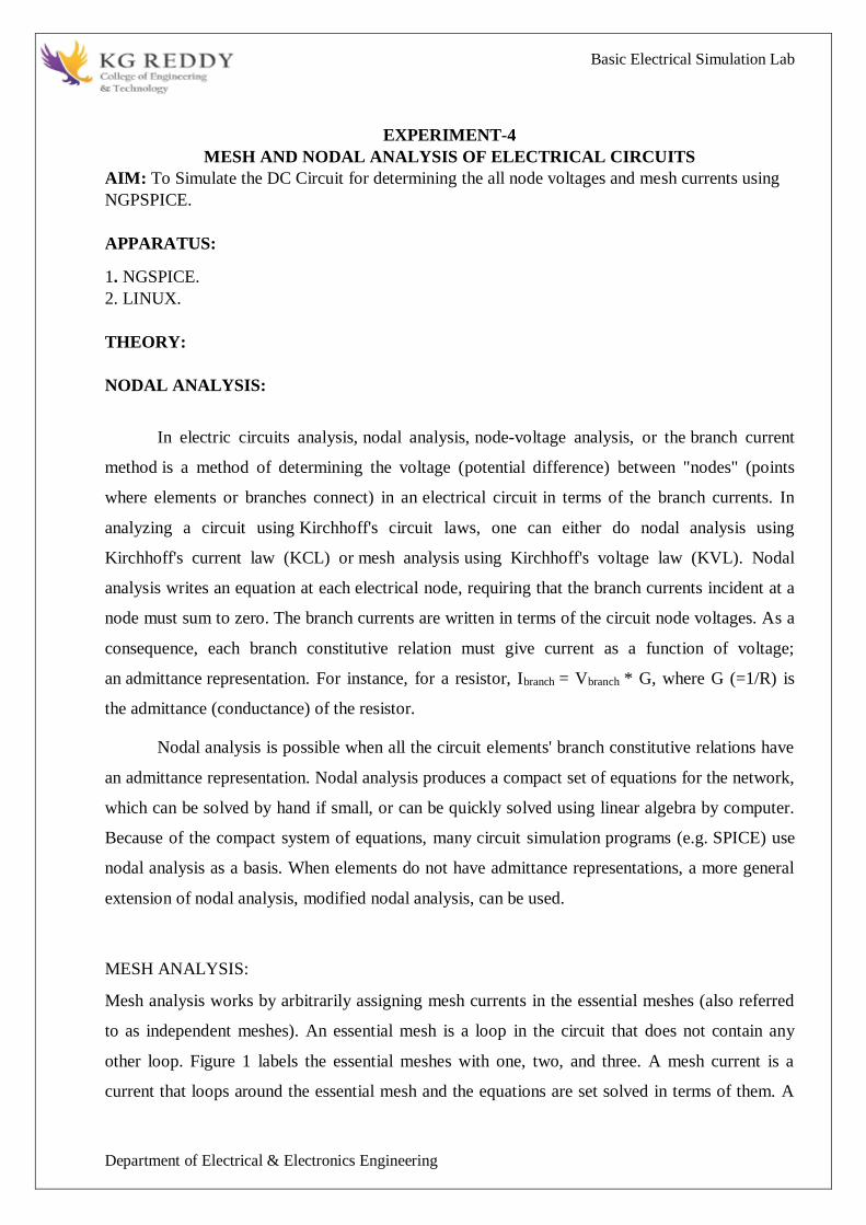
Basic Electrical Simulation Lab
Department of Electrical amp Electronics Engineering
EXPERIMENT-4
MESH AND NODAL ANALYSIS OF ELECTRICAL CIRCUITS
AIM To Simulate the DC Circuit for determining the all node voltages and mesh currents using
NGPSPICE
APPARATUS
1 NGSPICE
2 LINUX
THEORY
NODAL ANALYSIS
In electric circuits analysis nodal analysis node-voltage analysis or the branch current
method is a method of determining the voltage (potential difference) between nodes (points
where elements or branches connect) in an electrical circuit in terms of the branch currents In
analyzing a circuit using Kirchhoffs circuit laws one can either do nodal analysis using
Kirchhoffs current law (KCL) or mesh analysis using Kirchhoffs voltage law (KVL) Nodal
analysis writes an equation at each electrical node requiring that the branch currents incident at a
node must sum to zero The branch currents are written in terms of the circuit node voltages As a
consequence each branch constitutive relation must give current as a function of voltage
an admittance representation For instance for a resistor Ibranch = Vbranch G where G (=1R) is
the admittance (conductance) of the resistor
Nodal analysis is possible when all the circuit elements branch constitutive relations have
an admittance representation Nodal analysis produces a compact set of equations for the network
which can be solved by hand if small or can be quickly solved using linear algebra by computer
Because of the compact system of equations many circuit simulation programs (eg SPICE) use
nodal analysis as a basis When elements do not have admittance representations a more general
extension of nodal analysis modified nodal analysis can be used
MESH ANALYSIS
Mesh analysis works by arbitrarily assigning mesh currents in the essential meshes (also referred
to as independent meshes) An essential mesh is a loop in the circuit that does not contain any
other loop Figure 1 labels the essential meshes with one two and three A mesh current is a
current that loops around the essential mesh and the equations are set solved in terms of them A
Basic Electrical Simulation Lab
Department of Electrical amp Electronics Engineering
mesh current may not correspond to any physically flowing current but the physical currents are
easily found from them It is usual practice to have all the mesh currents loop in the same
direction This helps prevent errors when writing out the equations The convention is to have all
the mesh currents looping in a clockwise direction
Solving for mesh currents instead of directly applying Kirchhoffs current law and Kirchhoffs
voltage law can greatly reduce the amount of calculation required This is because there are fewer
mesh currents than there are physical branch currents
CIRCUIT DIAGRAM
PROGRAM
Vs 1 0 DC 20V
Ra 1 2 5k
Rb 2 0 4k
Rc 3 0 1k
Is 3 2 DC 20mA
DC
end
OUTPUT-
RESULT-
Basic Electrical Simulation Lab
Department of Electrical amp Electronics Engineering
EXPERIMENT-5
APPLICATION OF NETWORK THEOREMS TO ELECTRICAL NETWORKS
AIM To Simulate the different network theorems to electrical networks using NGPSPICE
APPARATUS
1 NGSPICE
2 LINUX
THEORY
THEVENINrsquoS THEOREM
The Theveninrsquos Theorem states that ldquoAny two terminals linear bilateral DC network can
be replaced by an equivalent circuit consisting of a voltage source Vth in series with all equivalent
resistance Rthrdquo
(OR)
Thevenins theorem states that ldquoin any two terminal linear bilateral network having a
number of voltage current sources and resistances can be replaced by a simple equivalent circuit
consisting of a single voltage source in series with a resistance where the value of the voltage
source is equal to the open circuit voltage across the two terminals of the network and the
resistance is the equivalent resistance measured between the terminals with all energy sources
replaced by their internal resistancesrdquo
NORTONrsquoS THEOREM
Nortons theorem States that ldquoin any two terminal linear bilateral network with current
sources voltage sources and resistances can be replaced by an equivalent circuit consisting of a
current source in parallel with a resistance The value of the current source is the short circuit
current between the two terminals of the network and the resistance is the equivalent resistance
measured between the terminals of the network with all the energy sources replaced by their
internal resistancesrdquo
SUPERPOSITION THEOREM
This theorem states that ldquoThe response (voltage or current) in any branch of a bilateral
linear circuit having more than one independent source equals the algebraic sum of the responses
caused by each independent source acting alone where all the other independent sources are
replaced by their internal resistancerdquo
Basic Electrical Simulation Lab
Department of Electrical amp Electronics Engineering
i1 2kΩ
+
5000
+
minus minus
+
100i1 20kΩ
minus
1 3
2
A given response in a network regulating from a number of independent sources(including
initial condition source) may be computed by summing the response to each individual source
with all other sources made in operative( reduced to zero voltage or zero current)
This statement describes the property homogeneity in linear networks So it is the
combined properties off additivity and homogeneity off linear network It is a result of the linear
relation between current and volt in circuits having linear impedances
MAX POWER TRANSFER THEOREM
Max power will be delivered by network to the load if the impedance of network is
Complex conjugate of load impedance and vice versa
(or)
The maximum transformer states that ldquoA load will received maximum power from a
linear bilateral network when its load resistance is exactly equal to the Theveninrsquos resistance
of network measured looking back into the terminals of network
PROGRAM
THEVENINS THEORM
2mV -
Find Thevenin equivalent circuit
V10 1 0 2M V
R12 1 1A 2K
V1A 1A 2 DC 0V
E20 2 0 3 0 2E-4
F30 3 0 V1A 100
R30 3 0 20K
RL 3 0 1G
TF v(3) v10
END
NODE VOLTAGE NODE VOLTAGE NODE VOLTAGE NODE VOLTAGE
Basic Electrical Simulation Lab
Department of Electrical amp Electronics Engineering
NORTONS THEORM
PROGRAM
Vs 1 0 DC 20V
R1 1 2 18k
Rb 2 0 22k
Rc 2 3 33k
Is 3 0 RL
DC
end
MAXIMUM POWER TRANSFER THEOREM
PROGRAM
VS 1 0 DC 100
R1 1 2 10
R2 2 0 30
R3 1 3 20
R4 3 0 40
RL 2 3 RLOAD 1
MODEL RLOAD RES(R=25)
DC RES RLOAD(R) 0001 40 001
TF V(23) VS
PROBE
END
Basic Electrical Simulation Lab
Department of Electrical amp Electronics Engineering
SUPERPOSITION THEOREM
Program FOR CIRCUIT 1 FOR CIRCUIT 2
VDC 1 2 DC 10V VDC 1 2 DC 10V VDC 1 2 DC 0V
R1 1 3 100 R1 1 3 100 R1 1 3 100
R2 3 4 200 R2 3 4 200 R2 3 4 200
R3 3 6 470 R3 3 6 470 R3 3 6 470
R4 2 0 560 R4 2 0 560 R4 2 0 560
R5 4 5 100 R5 4 0 100 R5 4 5 100
VX 5 0 DC 10V VY 6 0 DC 0V VY 6 0 DC 0V
VY 6 0 DC 0V OP OP
OP END END
END
OUTPUT-
RESULT-
Basic Electrical Simulation Lab
Department of Electrical amp Electronics Engineering
EXPERIMET-6
WAVEFORM SYNTHESIS USING LAPLACE TRANSFORM
AIM To perform waveform synthesis using Laplace Transforms of a given signal
APPARATUS
1 OCTAVE
2 LINUX
THEORY
Bilateral Laplace transform
When one says the Laplace transform without qualification the unilateral or one-sided
transform is normally intended The Laplace transform can be alternatively defined as the bilateral
Laplace transform or two-sided Laplace transform by extending the limits of integration to be the
entire real axis If that is done the common unilateral transform simply becomes a special case of
the bilateral transform where the definition of the function being transformed is multiplied by the
Heaviside step function The bilateral Laplace transform is defined as follows
Inverse Laplace transform
The inverse Laplace transform is given by the following complex integral which is known by
various names (the Bromwich integral the Fourier-Mellin integral and Mellins inverse formula)
Example
Let y(t)=exp(t)
We have
The integral converges if sgt1 The functions exp(t) and 1(s-1) are partner functions
Basic Electrical Simulation Lab
Department of Electrical amp Electronics Engineering
PROGRAM-
Laplace Transform
clc
clear all
close all
syms t
x=exp(-2t)heaviside(t)
y=laplace(x)
disp(Laplace Transform of input signal)
y
z=ilaplace(y)
disp(Inverse Laplace Transform of input signal)
z
PROCEDURE-
1 Open OCTAVE
2 Open new script
3 Type the program
4 Save in current directory
5 Compile and Run the program
6 For the output see command window Figure window
OUTPUT-
RESULT-
Basic Electrical Simulation Lab
Department of Electrical amp Electronics Engineering
EXPERIMENT-7
LOCATING THE ZEROS AND POLES AND PLOTTING THE
POLE ZERO MAPS IN S-PLANE AND Z-PLANE FOR THE GIVEN
TRANSFER FUNCTION
AIM To locating the zeros and poles and plotting the pole zero maps in s-plane and z-plane
for the given transfer function
APPARATUS
1 OCTAVE
2 LINUX
THEORY
A Transfer Function is the ratio of the output of a system to the input of a system in the Laplace
domain considering its initial conditions to be zero If we have an input function of X(s) and an
output function Y(s) we define the transfer function H(s) to be
transfer function is the Laplace transform of a system‟ s impulse response
Given a continuous-time transfer function in the Laplace domain H(s) or a discrete-time one in
the Z-domain H(z) a zero is any value of s or z such that the transfer function is zero and a pole
is any value of s or z such that the transfer function is infinite
Zeros1 The value(s) for z where the numerator of the transfer function equals zero 2 The
complex frequencies that make the overall gain of the filter transfer function zero
Poles 1 The value(s) for z where the denominator of the transfer function equals zero 2 The
omplex frequencies that make the overall gain of the filter transfer function
infinite
Z-transforms
the Z-transform converts a discrete time-domain signal which is a sequence of real or complex
numbers into a complex frequency-domain representationThe Z-transform like many other
integral transforms can be defined as either a one-sided or two-sided transform
Basic Electrical Simulation Lab
Department of Electrical amp Electronics Engineering
Bilateral Z-transform
The bilateral or two-sided Z-transform of a discrete-time signal x[n] is the function X(z)
defined as
Unilateral Z-transform
Alternatively in cases where x[n] is defined only for n ge 0 the single-sided or unilateral
Z-transform is defined as
In signal processing this definition is used when the signal is causal
The roots of the equation P(z) = 0 correspond to the zeros of X(z)
The roots of the equation Q(z) = 0 correspond to the poles of X(z)
PROGRAM-
locating poles of zero on s-plane
clc
clear all
close all
num=input(enter numerator co-efficients)
den=input(enter denominator co-efficients)
h=tf(numden)
poles=roots(den)
zeros=roots(num)
sgrid
pzmap(h)
grid on
title(locating poles of zeros on s-plane)
Basic Electrical Simulation Lab
Department of Electrical amp Electronics Engineering
locating poles ampzeros on z-plane
clc
clear all
close all
num=input(enter numerator coefficient)
den=input(enter denominator coefficient)
p=roots(den)
z=roots(num)
zplane(pz)
grid
title(locating poler and zeros on s-plane)
PROCEDURE-
1 Open OCTAVE
2 Open new script
3 Type the program
4 Save in current directory
5 Compile and Run the program
6 For the output see command window Figure window
OUTPUT-
RESULT-
Basic Electrical Simulation Lab
Department of Electrical amp Electronics Engineering
EXPERIMENT-8
SIMULATION OF DC CIRCUITS
AIM To Simulate the DC network using PSPICE
APPARATUS
1 NGSPICE
2 LINUX
THEORY
Generally speaking network analysis is any structured technique used to mathematically
analyze a circuit (a ldquonetworkrdquo of interconnected components) Quite often the technician or
engineer will encounter circuits containing multiple sources of power or component
configurations which defy simplification by seriesparallel analysis techniques In those cases he
or she will be forced to use other means This chapter presents a few techniques useful in
analyzing such complex circuits
To analyse the above circuit one would first find the equivalent of R2 and R3 in parallel
then add R1 in series to arrive at a total resistance Then taking the voltage of battery B1 with
that total circuit resistance the total current could be calculated through the use of Ohmrsquos
Law (I=ER) then that current figure used to calculate voltage drops in the circuit All in all a
fairly simple procedure However the addition of just one more battery could change all of that
PROGRAM
Basic Electrical Simulation Lab
Department of Electrical amp Electronics Engineering
Vs 1 0 DC 20V
Ra 1 2 5k
Rb 2 0 4k
Rc 3 0 1k
Is 3 2 DC 20mA
DC
end
OUTPUT-
RESULT-
Basic Electrical Simulation Lab
Department of Electrical amp Electronics Engineering
EXPERIMENT-9
TRANSIENT ANALYSIS
AIM To find out the transient response by simulation of RLC circuits Using NGSPICE
APPARATUS
1 NGSPICE
2 LINUX
THEORY
The transient simulation is the calculation of a networks response on arbitrary excitations The
results are network quantities (branch currents and node voltages) as a function of time
Substantial for the transient analysis is the consideration of energy storing components ie
inductors and capacitorsThe relations between current and voltage of ideal capacitors and
inductors are given by
(61)
Or in terms of differential equations
(62)
To calculate these quantities in a computer program numerical integration methods are required
With the current-voltage relations of these components at hand it is possible to apply the modified
nodal analysis algorithm in order to calculate the networks response This means the transient
analysis attempts to find an approximation to the analytical solution at discrete time points using
numeric integration
CIRCUIT DIAGRAM
Basic Electrical Simulation Lab
Department of Electrical amp Electronics Engineering
PROGRAM
VIN1 1 0 PWL(0 0 1NS 1V 1MS 1V)
VIN2 4 0 PWL(0 0 1NS 1V 1MS 1V)
VIN3 7 0 PWL(0 0 1NS 1V 1MS 1V)
R1 1 2 2
R2 4 5 1
R3 7 8 8
L1 2 3 50UH
L2 5 6 50UH
L3 8 9 50UH
C1 3 0 10UF
C2 6 0 10UF
C3 9 0 10UF
TRAN 1US 400US
PLOT TRAN V(3) V(6) V(9)
PROBE
END
OUTPUT-
RESULT-
Basic Electrical Simulation Lab
Department of Electrical amp Electronics Engineering
EXPERIMENT-10
SIMULATION OF SINGLE PHASE DIODE BRIDGE RECTIFIERS WITH FILTER FOR
R amp RL LOAD
AIM To analyze the simulation of 1-Oslash diode bridge rectifiers with filter for R amp RL load using
NGSPICE
APPARATUS
1 NGSPICE
2 LINUX
THEORY
A bridge rectifier circuit is a common part of the electronic power supplies
Many electronic circuits require rectified DC power supply for powering the various electronic
basic components from available AC mains supply We can find this rectifier in a wide variety of
electronic AC power devices like home appliances motor controllers modulation process
welding applications etc
A Bridge rectifier is an Alternating Current (AC) to Direct Current (DC) converter that
rectifies mains AC input to DC output Bridge Rectifiers are widely used in power supplies that
provide necessary DC voltage for the electronic components or devices They can be constructed
with four or more diodes or any other controlled solid state switches Depending on the load
current requirements a proper bridge rectifier is selected Componentsrsquo ratings and specifications
breakdown voltage temperature ranges transient current rating forward current rating mounting
requirements and other considerations are taken into account while selecting a rectifier power
supply for an appropriate electronic circuitrsquos application
Bride rectifiers are classified into several types based on these factors type of supply
controlling capability bride circuitrsquos configurations etc Bridge rectifiers are mainly classified
into single and three phase rectifiers Both these types are further classified into uncontrolled half
controlled and full controlled rectifiers
Basic Electrical Simulation Lab
Department of Electrical amp Electronics Engineering
Program
VS 1 0 SIN(0 1697V 60HZ)
DF 5 4 DMOD
R1 4 7 10
L1 7 8 20MH
C1 4 6 793UF
RX 6 5 01
VX 8 5 DC 10V
VY 2 1 DC 0V
D1 2 4 DMOD
D2 5 3 DMOD
D3 3 4 DMOD
D4 5 2 DMOD
MODEL DMOD D( IS=22E-15 BV=1800 TT=0)
TRAN 10US 100MS 166MS
PROBE
FOUR 120HZ I(VX)
END
OUTPUT-
RESULT-
Basic Electrical Simulation Lab
Department of Electrical amp Electronics Engineering
EXPERIMENT-11
SIMULATION OF THREE PHASE DIODE BRIDGE RECTIFIERS WITH R RL LOAD
AIM To analyze the simulation of 3-Oslash diode bridge rectifiers with filter for R amp RL load using
NGSPICE
APPARATUS
1 NGSPICE
2 LINUX
THEORY
Three phase half controlled bridge converters amp fully controlled bridge converters are used
extensively in industrial applications up to about 15kW of output power The Three phase
controlled rectifiers provide a maximum dc output of
vdc(max)=2vm prod
The output ripple frequency is equal to the twice the ac supply frequency The single phase
full wave controlled rectifiers provide two output pulses during every input supply cycle
and hence are referred to as two pulse converters
Three phase converters are 3-phase controlled rectifiers which are used to convert ac input
power supply into dc output power across the load
Features of 3-phase controlled rectifiers are
Operate from 3 phase ac supply voltage
They provide higher dc output voltage and higher dc output power
Higher output voltage ripple frequency
Filtering requirements are simplified for smoothing out load voltage and load
current
Three phase controlled rectifiers are extensively used in high power variable speed
industrial dc drives
Basic Electrical Simulation Lab
Department of Electrical amp Electronics Engineering
Program
VAN 1 0 SIN(0V 200V 50HZ 0 0 0)
VBN 2 0 SIN(0V 200V 50HZ 0 0 -120)
VCN 3 0 SIN(0V 200V 50HZ 0 0 -240)
R 7 9 20
L 9 10 55MH
VX 10 8 DC 0V
VY 1 4 DC 0V
D1 4 7 DMOD
D2 8 2 DMOD
D3 3 7 DMOD
D4 8 4 DMOD
D5 2 7 DMOD
D6 8 3 DMOD
MODEL DMOD D(IS=22E-15 BV=1800V TT=0)
TRAN 5US 50MS 2166MS
PROBE
END
OUTPUT-
RESULT-
Basic Electrical Simulation Lab
Department of Electrical amp Electronics Engineering
EXPERIMENT-12
DESIGN OF LOW PASS AND HIGH PASS FILTERS
AIM To analyze the simulation of 3-Oslash diode bridge rectifiers with filter for R amp RL load using
NGSPICE
APPARATUS
1 OCTAVE
2 LINUX
THEORY
A filter is a circuit that has designed to pass a specified band of frequencies while attenuating all
signals outside this band Active filters employ transistors or op-amps plus resistors inductors
and capacitors There are four types of filters low-pass high-pass band-pass and band-
elimination (also referred to as band-reject or notch) filters Figure 71 illustrates frequency-
response plot for the four types of filters A low-pass filter is a circuit that has a constant output
voltage from dc up to a cutoff frequency fc As the frequency increases above fc the output
voltage is attenuated (decreases) Figure 71(a) is a plot of magnitude of the output voltage of a
low-pass filter versus frequency The range of frequencies that are transmitted is known as the
pass-band The range of frequencies that are attenuated is known as the stop-band The cutoff
frequency fc is also called the 0707 frequency the 3-dB frequency the corner frequency or the
break frequency High-pass filters attenuate the output voltage for all frequencies below the cutoff
frequency fc Above fc the magnitude of the output voltage is constant Figure 71(b) is the plot
for ideal and practical high-pass filters Band-pass filters pass only a band of frequencies while
attenuating all frequencies outside the band Band-elimination filters perform in an exactly
opposite way that is band-elimination filters reject a specified band of frequencies while passing
all frequencies outside the band Typical frequency-response plots for band-pass and band-
elimination filters are shown in Figure 71(c) and (d) In many filter applications it is necessary
for the closed-loop gain to be as close to 1 as possible within the pass band The Butterworth filter
is best suited for this type of application The Butterworth filter is also called a maximally flat or
flat-flat filter and all filter in this experiment will be of the Butterworth type Figure 72 shows
the ideal and the practical frequency response for three types of Butterworth filters As the roll-
offs become steeper they approach the ideal filter more closely
Basic Electrical Simulation Lab
Department of Electrical amp Electronics Engineering
PROGRAM
LOW PASS FILTER
N = 100 FIR filter order
Fp = 20e3 20 kHz passband-edge frequency
Fs = 96e3 96 kHz sampling frequency
Rp = 000057565 Corresponds to 001 dB peak-to-peak ripple
Rst = 1e-4 Corresponds to 80 dB stopband attenuation
eqnum = firceqrip(NFp(Fs2)[Rp Rst]passedge) eqnum = vec of coeffs
fvtool(eqnumFsFsColorWhite) Visualize filter
HIGH PASS FILTER
Fstop = 350
Fpass = 400
Astop = 65
Apass = 05
Fs = 1e3
d = designfilt(highpassfirStopbandFrequencyFstop
PassbandFrequencyFpassStopbandAttenuationAstop
PassbandRippleApassSampleRateFsDesignMethodequiripple)
fvtool(d)
OUTPUT-
RESULT-
Basic Electrical Simulation Lab
Department of Electrical amp Electronics Engineering
EXPERIMENT-13
FINDING THE EVEN AND ODD PARTS OF SIGNAL SEQUENCE AND REAL AND
IMAGINARY PARTS OF SIGNAL
AIM
program for finding even and odd parts of sequences Using OCTAVE Softwareamp
program for finding real and imaginary parts of sequences Using OCTAVE Software
APPARATUS
1 OCTAVE
2 LINUX
THEORY
Even and Odd Signal
One of characteristics of signal is symmetry that may be useful for signal analysis Even signals
are symmetric around vertical axis and Odd signals are symmetric about origin
Even Signal A signal is referred to as an even if it is identical to its time-reversed counterparts
x(t) = x(-t)
Odd Signal A signal is odd if x(t) = -x(-t)
An odd signal must be 0 at t=0 in other words odd signal passes the origin
Using the definition of even and odd signal any signal may be decomposed into a sum of its even
part xe(t) and its odd part xo(t) as follows
x(t)=xe(t)+xo(t)
x(t)=12x(t)+x(-t) +12x(t)-x(-t)
where
xe(t)=12x(t)+x(-t) ampxo(t)=12x(t)-x(-t)
It is an important fact because it is relative concept of Fourier series In Fourier series aperiodic
signal can be broken into a sum of sine and cosine signals Notice that sine function is odd signal
and cosine function is even signal
ENERGY AND POWER SIGNAL
A signal can be categorized into energy signal or power
signal An energy signal has a finite energy 0 lt E lt 1049279 In other words energy signals have
values only in the limited time duration For example a signal having only one square pulse is
energy signal A signal that decays exponentially has finite energy so it is also an energy signal
The power of an energy signal is 0 because of dividing finite energy by infinite time (or length)
If x(t) is a real-valued signal with Fourier transform X(f) and u(f) is the Heaviside step function
Basic Electrical Simulation Lab
Department of Electrical amp Electronics Engineering
then the function
contains only the non-negative frequency components of X(f) And the operation is reversible due
to the Hermitian property of X(f)
X(f) denotes the complex conjugate of X(f)
The inverse Fourier transform of Xa(f) is the analytic signal
where x^(t) is the Hilbert transform of x(t) and J is the imaginary unit
Basic Electrical Simulation Lab
Department of Electrical amp Electronics Engineering
PROGRAM-
Evenoddrealimaginary parts of a sequences
clc
clear all
close all
h=input(enter noof samples)
m=(h-1)2
n=-mm
x=input(enter sample values)
subplot(411)
stem(nxg)
xlabel(time)
ylabel(amplitude)
title(original sequence)
xmir=fliplr(x)
subplot(412)
stem(nxmirr)
xlabel(time)
ylabel(amplitude)
title(folded sequence)
even part of sequence
xeven=(x+xmir)2
subplot(413)
stem(nxevenr)
xlabel(time)
ylabel(amplitude)
title(even part of sequence)
odd part of sequence
xodd=(x-xmir)2
subplot(414)
stem(nxoddg)
xlabel(time)
ylabel(amplitude)
title(odd part of sequence)
Basic Electrical Simulation Lab
Department of Electrical amp Electronics Engineering
RealampImaginary parts of a sequences
clc
clear all
close all
y=input(enter complex numbers)
yreal=real(y)
disp(real values of y)
yreal
yimag=imag(y)
disp(imaginary values of y)
yimag
PROCEDURE-
1 Open OCTAVE
2 Open new script
3 Type the program
4 Save in current directory
5 Compile and Run the program
6 For the output see command window Figure window
OUTPUT-
RESULT-
Basic Electrical Simulation Lab
Department of Electrical amp Electronics Engineering
EXPERIMENT-14
FINDING THE FOURIER TRANSFORM OF A GIVEN SIGNAL AND PLOTTING ITS
MAGNITUDE AND PHASE SPECTRUM
AIM
Program for finding the fourier transform of a given signal Using OCTAVE Software amp Plotting
Its Magnitude And Phase Spectrum Using OCTAVE Software
APPARATUS
1 OCTAVE
2 LINUX
THEORY
The Fourier transform (FT) decomposes a function of time (a signal) into the
frequencies that make it up in a way similar to how a musical chord can be expressed as the
frequencies (or pitches) of its constituent notes The Fourier transform of a function of time itself
is a complex-valued function of frequency whose absolute value represents the amount of that
frequency present in the original function and whose complex argument is the phase offset of the
basic sinusoid in that frequency The Fourier transform is called the frequency domain
representation of the original signal The term Fourier transform refers to both the frequency
domain representation and the mathematical operation that associates the frequency domain
representation to a function of time The Fourier transform is not limited to functions of time but
in order to have a unified language the domain of the original function is commonly referred to as
the time domain For many functions of practical interest one can define an operation that
reverses this the inverse Fourier transformation also called Fourier synthesis of a frequency
domain representation combines the contributions of all the different frequencies to recover the
original function of time
Linear operations performed in one domain (time or frequency) have corresponding
operations in the other domain which are sometimes easier to perform The operation
of differentiation in the time domain corresponds to multiplication by the frequency[remark 1] so
some differential equations are easier to analyze in the frequency domain Also convolution in the
time domain corresponds to ordinary multiplication in the frequency domain Concretely this
means that any linear time-invariant system such as a filter applied to a signal can be expressed
relatively simply as an operation on frequencies After performing the desired operations
transformation of the result can be made back to the time domain Harmonic analysis is the
systematic study of the relationship between the frequency and time domains including the kinds
Basic Electrical Simulation Lab
Department of Electrical amp Electronics Engineering
of functions or operations that are simpler in one or the other and has deep connections to many
areas of modern mathematics
PROGRAM
Fs = 1000 Sampling frequency
T = 1Fs Sampling period
L = 1500 Length of signal
t = (0L-1)T Time vector
S = 07sin(2pi50t) + sin(2pi120t)
X = S + 2randn(size(t))
plot(1000t(150)X(150))
title(Signal Corrupted with Zero-Mean Random Noise)
xlabel(t (milliseconds))
ylabel(X(t))
Y = fft(X)
P2 = abs(YL)
P1 = P2(1L2+1)
P1(2end-1) = 2P1(2end-1)
f = Fs(0(L2))L
plot(fP1)
title(Single-Sided Amplitude Spectrum of X(t))
xlabel(f (Hz))
ylabel(|P1(f)|)
Y = fft(S)
P2 = abs(YL)
P1 = P2(1L2+1)
P1(2end-1) = 2P1(2end-1)
plot(fP1)
title(Single-Sided Amplitude Spectrum of S(t))
xlabel(f (Hz))
ylabel(|P1(f)|)
OUTPUT-
RESULT-
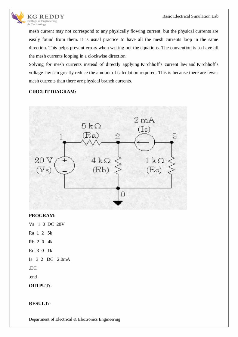
Basic Electrical Simulation Lab
Department of Electrical amp Electronics Engineering
EXPERIMENT-5
APPLICATION OF NETWORK THEOREMS TO ELECTRICAL NETWORKS
AIM To Simulate the different network theorems to electrical networks using NGPSPICE
APPARATUS
1 NGSPICE
2 LINUX
THEORY
THEVENINrsquoS THEOREM
The Theveninrsquos Theorem states that ldquoAny two terminals linear bilateral DC network can
be replaced by an equivalent circuit consisting of a voltage source Vth in series with all equivalent
resistance Rthrdquo
(OR)
Thevenins theorem states that ldquoin any two terminal linear bilateral network having a
number of voltage current sources and resistances can be replaced by a simple equivalent circuit
consisting of a single voltage source in series with a resistance where the value of the voltage
source is equal to the open circuit voltage across the two terminals of the network and the
resistance is the equivalent resistance measured between the terminals with all energy sources
replaced by their internal resistancesrdquo
NORTONrsquoS THEOREM
Nortons theorem States that ldquoin any two terminal linear bilateral network with current
sources voltage sources and resistances can be replaced by an equivalent circuit consisting of a
current source in parallel with a resistance The value of the current source is the short circuit
current between the two terminals of the network and the resistance is the equivalent resistance
measured between the terminals of the network with all the energy sources replaced by their
internal resistancesrdquo
SUPERPOSITION THEOREM
This theorem states that ldquoThe response (voltage or current) in any branch of a bilateral
linear circuit having more than one independent source equals the algebraic sum of the responses
caused by each independent source acting alone where all the other independent sources are
replaced by their internal resistancerdquo
Basic Electrical Simulation Lab
Department of Electrical amp Electronics Engineering
i1 2kΩ
+
5000
+
minus minus
+
100i1 20kΩ
minus
1 3
2
A given response in a network regulating from a number of independent sources(including
initial condition source) may be computed by summing the response to each individual source
with all other sources made in operative( reduced to zero voltage or zero current)
This statement describes the property homogeneity in linear networks So it is the
combined properties off additivity and homogeneity off linear network It is a result of the linear
relation between current and volt in circuits having linear impedances
MAX POWER TRANSFER THEOREM
Max power will be delivered by network to the load if the impedance of network is
Complex conjugate of load impedance and vice versa
(or)
The maximum transformer states that ldquoA load will received maximum power from a
linear bilateral network when its load resistance is exactly equal to the Theveninrsquos resistance
of network measured looking back into the terminals of network
PROGRAM
THEVENINS THEORM
2mV -
Find Thevenin equivalent circuit
V10 1 0 2M V
R12 1 1A 2K
V1A 1A 2 DC 0V
E20 2 0 3 0 2E-4
F30 3 0 V1A 100
R30 3 0 20K
RL 3 0 1G
TF v(3) v10
END
NODE VOLTAGE NODE VOLTAGE NODE VOLTAGE NODE VOLTAGE
Basic Electrical Simulation Lab
Department of Electrical amp Electronics Engineering
NORTONS THEORM
PROGRAM
Vs 1 0 DC 20V
R1 1 2 18k
Rb 2 0 22k
Rc 2 3 33k
Is 3 0 RL
DC
end
MAXIMUM POWER TRANSFER THEOREM
PROGRAM
VS 1 0 DC 100
R1 1 2 10
R2 2 0 30
R3 1 3 20
R4 3 0 40
RL 2 3 RLOAD 1
MODEL RLOAD RES(R=25)
DC RES RLOAD(R) 0001 40 001
TF V(23) VS
PROBE
END
Basic Electrical Simulation Lab
Department of Electrical amp Electronics Engineering
SUPERPOSITION THEOREM
Program FOR CIRCUIT 1 FOR CIRCUIT 2
VDC 1 2 DC 10V VDC 1 2 DC 10V VDC 1 2 DC 0V
R1 1 3 100 R1 1 3 100 R1 1 3 100
R2 3 4 200 R2 3 4 200 R2 3 4 200
R3 3 6 470 R3 3 6 470 R3 3 6 470
R4 2 0 560 R4 2 0 560 R4 2 0 560
R5 4 5 100 R5 4 0 100 R5 4 5 100
VX 5 0 DC 10V VY 6 0 DC 0V VY 6 0 DC 0V
VY 6 0 DC 0V OP OP
OP END END
END
OUTPUT-
RESULT-
Basic Electrical Simulation Lab
Department of Electrical amp Electronics Engineering
EXPERIMET-6
WAVEFORM SYNTHESIS USING LAPLACE TRANSFORM
AIM To perform waveform synthesis using Laplace Transforms of a given signal
APPARATUS
1 OCTAVE
2 LINUX
THEORY
Bilateral Laplace transform
When one says the Laplace transform without qualification the unilateral or one-sided
transform is normally intended The Laplace transform can be alternatively defined as the bilateral
Laplace transform or two-sided Laplace transform by extending the limits of integration to be the
entire real axis If that is done the common unilateral transform simply becomes a special case of
the bilateral transform where the definition of the function being transformed is multiplied by the
Heaviside step function The bilateral Laplace transform is defined as follows
Inverse Laplace transform
The inverse Laplace transform is given by the following complex integral which is known by
various names (the Bromwich integral the Fourier-Mellin integral and Mellins inverse formula)
Example
Let y(t)=exp(t)
We have
The integral converges if sgt1 The functions exp(t) and 1(s-1) are partner functions
Basic Electrical Simulation Lab
Department of Electrical amp Electronics Engineering
PROGRAM-
Laplace Transform
clc
clear all
close all
syms t
x=exp(-2t)heaviside(t)
y=laplace(x)
disp(Laplace Transform of input signal)
y
z=ilaplace(y)
disp(Inverse Laplace Transform of input signal)
z
PROCEDURE-
1 Open OCTAVE
2 Open new script
3 Type the program
4 Save in current directory
5 Compile and Run the program
6 For the output see command window Figure window
OUTPUT-
RESULT-
Basic Electrical Simulation Lab
Department of Electrical amp Electronics Engineering
EXPERIMENT-7
LOCATING THE ZEROS AND POLES AND PLOTTING THE
POLE ZERO MAPS IN S-PLANE AND Z-PLANE FOR THE GIVEN
TRANSFER FUNCTION
AIM To locating the zeros and poles and plotting the pole zero maps in s-plane and z-plane
for the given transfer function
APPARATUS
1 OCTAVE
2 LINUX
THEORY
A Transfer Function is the ratio of the output of a system to the input of a system in the Laplace
domain considering its initial conditions to be zero If we have an input function of X(s) and an
output function Y(s) we define the transfer function H(s) to be
transfer function is the Laplace transform of a system‟ s impulse response
Given a continuous-time transfer function in the Laplace domain H(s) or a discrete-time one in
the Z-domain H(z) a zero is any value of s or z such that the transfer function is zero and a pole
is any value of s or z such that the transfer function is infinite
Zeros1 The value(s) for z where the numerator of the transfer function equals zero 2 The
complex frequencies that make the overall gain of the filter transfer function zero
Poles 1 The value(s) for z where the denominator of the transfer function equals zero 2 The
omplex frequencies that make the overall gain of the filter transfer function
infinite
Z-transforms
the Z-transform converts a discrete time-domain signal which is a sequence of real or complex
numbers into a complex frequency-domain representationThe Z-transform like many other
integral transforms can be defined as either a one-sided or two-sided transform
Basic Electrical Simulation Lab
Department of Electrical amp Electronics Engineering
Bilateral Z-transform
The bilateral or two-sided Z-transform of a discrete-time signal x[n] is the function X(z)
defined as
Unilateral Z-transform
Alternatively in cases where x[n] is defined only for n ge 0 the single-sided or unilateral
Z-transform is defined as
In signal processing this definition is used when the signal is causal
The roots of the equation P(z) = 0 correspond to the zeros of X(z)
The roots of the equation Q(z) = 0 correspond to the poles of X(z)
PROGRAM-
locating poles of zero on s-plane
clc
clear all
close all
num=input(enter numerator co-efficients)
den=input(enter denominator co-efficients)
h=tf(numden)
poles=roots(den)
zeros=roots(num)
sgrid
pzmap(h)
grid on
title(locating poles of zeros on s-plane)
Basic Electrical Simulation Lab
Department of Electrical amp Electronics Engineering
locating poles ampzeros on z-plane
clc
clear all
close all
num=input(enter numerator coefficient)
den=input(enter denominator coefficient)
p=roots(den)
z=roots(num)
zplane(pz)
grid
title(locating poler and zeros on s-plane)
PROCEDURE-
1 Open OCTAVE
2 Open new script
3 Type the program
4 Save in current directory
5 Compile and Run the program
6 For the output see command window Figure window
OUTPUT-
RESULT-
Basic Electrical Simulation Lab
Department of Electrical amp Electronics Engineering
EXPERIMENT-8
SIMULATION OF DC CIRCUITS
AIM To Simulate the DC network using PSPICE
APPARATUS
1 NGSPICE
2 LINUX
THEORY
Generally speaking network analysis is any structured technique used to mathematically
analyze a circuit (a ldquonetworkrdquo of interconnected components) Quite often the technician or
engineer will encounter circuits containing multiple sources of power or component
configurations which defy simplification by seriesparallel analysis techniques In those cases he
or she will be forced to use other means This chapter presents a few techniques useful in
analyzing such complex circuits
To analyse the above circuit one would first find the equivalent of R2 and R3 in parallel
then add R1 in series to arrive at a total resistance Then taking the voltage of battery B1 with
that total circuit resistance the total current could be calculated through the use of Ohmrsquos
Law (I=ER) then that current figure used to calculate voltage drops in the circuit All in all a
fairly simple procedure However the addition of just one more battery could change all of that
PROGRAM
Basic Electrical Simulation Lab
Department of Electrical amp Electronics Engineering
Vs 1 0 DC 20V
Ra 1 2 5k
Rb 2 0 4k
Rc 3 0 1k
Is 3 2 DC 20mA
DC
end
OUTPUT-
RESULT-
Basic Electrical Simulation Lab
Department of Electrical amp Electronics Engineering
EXPERIMENT-9
TRANSIENT ANALYSIS
AIM To find out the transient response by simulation of RLC circuits Using NGSPICE
APPARATUS
1 NGSPICE
2 LINUX
THEORY
The transient simulation is the calculation of a networks response on arbitrary excitations The
results are network quantities (branch currents and node voltages) as a function of time
Substantial for the transient analysis is the consideration of energy storing components ie
inductors and capacitorsThe relations between current and voltage of ideal capacitors and
inductors are given by
(61)
Or in terms of differential equations
(62)
To calculate these quantities in a computer program numerical integration methods are required
With the current-voltage relations of these components at hand it is possible to apply the modified
nodal analysis algorithm in order to calculate the networks response This means the transient
analysis attempts to find an approximation to the analytical solution at discrete time points using
numeric integration
CIRCUIT DIAGRAM
Basic Electrical Simulation Lab
Department of Electrical amp Electronics Engineering
PROGRAM
VIN1 1 0 PWL(0 0 1NS 1V 1MS 1V)
VIN2 4 0 PWL(0 0 1NS 1V 1MS 1V)
VIN3 7 0 PWL(0 0 1NS 1V 1MS 1V)
R1 1 2 2
R2 4 5 1
R3 7 8 8
L1 2 3 50UH
L2 5 6 50UH
L3 8 9 50UH
C1 3 0 10UF
C2 6 0 10UF
C3 9 0 10UF
TRAN 1US 400US
PLOT TRAN V(3) V(6) V(9)
PROBE
END
OUTPUT-
RESULT-
Basic Electrical Simulation Lab
Department of Electrical amp Electronics Engineering
EXPERIMENT-10
SIMULATION OF SINGLE PHASE DIODE BRIDGE RECTIFIERS WITH FILTER FOR
R amp RL LOAD
AIM To analyze the simulation of 1-Oslash diode bridge rectifiers with filter for R amp RL load using
NGSPICE
APPARATUS
1 NGSPICE
2 LINUX
THEORY
A bridge rectifier circuit is a common part of the electronic power supplies
Many electronic circuits require rectified DC power supply for powering the various electronic
basic components from available AC mains supply We can find this rectifier in a wide variety of
electronic AC power devices like home appliances motor controllers modulation process
welding applications etc
A Bridge rectifier is an Alternating Current (AC) to Direct Current (DC) converter that
rectifies mains AC input to DC output Bridge Rectifiers are widely used in power supplies that
provide necessary DC voltage for the electronic components or devices They can be constructed
with four or more diodes or any other controlled solid state switches Depending on the load
current requirements a proper bridge rectifier is selected Componentsrsquo ratings and specifications
breakdown voltage temperature ranges transient current rating forward current rating mounting
requirements and other considerations are taken into account while selecting a rectifier power
supply for an appropriate electronic circuitrsquos application
Bride rectifiers are classified into several types based on these factors type of supply
controlling capability bride circuitrsquos configurations etc Bridge rectifiers are mainly classified
into single and three phase rectifiers Both these types are further classified into uncontrolled half
controlled and full controlled rectifiers
Basic Electrical Simulation Lab
Department of Electrical amp Electronics Engineering
Program
VS 1 0 SIN(0 1697V 60HZ)
DF 5 4 DMOD
R1 4 7 10
L1 7 8 20MH
C1 4 6 793UF
RX 6 5 01
VX 8 5 DC 10V
VY 2 1 DC 0V
D1 2 4 DMOD
D2 5 3 DMOD
D3 3 4 DMOD
D4 5 2 DMOD
MODEL DMOD D( IS=22E-15 BV=1800 TT=0)
TRAN 10US 100MS 166MS
PROBE
FOUR 120HZ I(VX)
END
OUTPUT-
RESULT-
Basic Electrical Simulation Lab
Department of Electrical amp Electronics Engineering
EXPERIMENT-11
SIMULATION OF THREE PHASE DIODE BRIDGE RECTIFIERS WITH R RL LOAD
AIM To analyze the simulation of 3-Oslash diode bridge rectifiers with filter for R amp RL load using
NGSPICE
APPARATUS
1 NGSPICE
2 LINUX
THEORY
Three phase half controlled bridge converters amp fully controlled bridge converters are used
extensively in industrial applications up to about 15kW of output power The Three phase
controlled rectifiers provide a maximum dc output of
vdc(max)=2vm prod
The output ripple frequency is equal to the twice the ac supply frequency The single phase
full wave controlled rectifiers provide two output pulses during every input supply cycle
and hence are referred to as two pulse converters
Three phase converters are 3-phase controlled rectifiers which are used to convert ac input
power supply into dc output power across the load
Features of 3-phase controlled rectifiers are
Operate from 3 phase ac supply voltage
They provide higher dc output voltage and higher dc output power
Higher output voltage ripple frequency
Filtering requirements are simplified for smoothing out load voltage and load
current
Three phase controlled rectifiers are extensively used in high power variable speed
industrial dc drives
Basic Electrical Simulation Lab
Department of Electrical amp Electronics Engineering
Program
VAN 1 0 SIN(0V 200V 50HZ 0 0 0)
VBN 2 0 SIN(0V 200V 50HZ 0 0 -120)
VCN 3 0 SIN(0V 200V 50HZ 0 0 -240)
R 7 9 20
L 9 10 55MH
VX 10 8 DC 0V
VY 1 4 DC 0V
D1 4 7 DMOD
D2 8 2 DMOD
D3 3 7 DMOD
D4 8 4 DMOD
D5 2 7 DMOD
D6 8 3 DMOD
MODEL DMOD D(IS=22E-15 BV=1800V TT=0)
TRAN 5US 50MS 2166MS
PROBE
END
OUTPUT-
RESULT-
Basic Electrical Simulation Lab
Department of Electrical amp Electronics Engineering
EXPERIMENT-12
DESIGN OF LOW PASS AND HIGH PASS FILTERS
AIM To analyze the simulation of 3-Oslash diode bridge rectifiers with filter for R amp RL load using
NGSPICE
APPARATUS
1 OCTAVE
2 LINUX
THEORY
A filter is a circuit that has designed to pass a specified band of frequencies while attenuating all
signals outside this band Active filters employ transistors or op-amps plus resistors inductors
and capacitors There are four types of filters low-pass high-pass band-pass and band-
elimination (also referred to as band-reject or notch) filters Figure 71 illustrates frequency-
response plot for the four types of filters A low-pass filter is a circuit that has a constant output
voltage from dc up to a cutoff frequency fc As the frequency increases above fc the output
voltage is attenuated (decreases) Figure 71(a) is a plot of magnitude of the output voltage of a
low-pass filter versus frequency The range of frequencies that are transmitted is known as the
pass-band The range of frequencies that are attenuated is known as the stop-band The cutoff
frequency fc is also called the 0707 frequency the 3-dB frequency the corner frequency or the
break frequency High-pass filters attenuate the output voltage for all frequencies below the cutoff
frequency fc Above fc the magnitude of the output voltage is constant Figure 71(b) is the plot
for ideal and practical high-pass filters Band-pass filters pass only a band of frequencies while
attenuating all frequencies outside the band Band-elimination filters perform in an exactly
opposite way that is band-elimination filters reject a specified band of frequencies while passing
all frequencies outside the band Typical frequency-response plots for band-pass and band-
elimination filters are shown in Figure 71(c) and (d) In many filter applications it is necessary
for the closed-loop gain to be as close to 1 as possible within the pass band The Butterworth filter
is best suited for this type of application The Butterworth filter is also called a maximally flat or
flat-flat filter and all filter in this experiment will be of the Butterworth type Figure 72 shows
the ideal and the practical frequency response for three types of Butterworth filters As the roll-
offs become steeper they approach the ideal filter more closely
Basic Electrical Simulation Lab
Department of Electrical amp Electronics Engineering
PROGRAM
LOW PASS FILTER
N = 100 FIR filter order
Fp = 20e3 20 kHz passband-edge frequency
Fs = 96e3 96 kHz sampling frequency
Rp = 000057565 Corresponds to 001 dB peak-to-peak ripple
Rst = 1e-4 Corresponds to 80 dB stopband attenuation
eqnum = firceqrip(NFp(Fs2)[Rp Rst]passedge) eqnum = vec of coeffs
fvtool(eqnumFsFsColorWhite) Visualize filter
HIGH PASS FILTER
Fstop = 350
Fpass = 400
Astop = 65
Apass = 05
Fs = 1e3
d = designfilt(highpassfirStopbandFrequencyFstop
PassbandFrequencyFpassStopbandAttenuationAstop
PassbandRippleApassSampleRateFsDesignMethodequiripple)
fvtool(d)
OUTPUT-
RESULT-
Basic Electrical Simulation Lab
Department of Electrical amp Electronics Engineering
EXPERIMENT-13
FINDING THE EVEN AND ODD PARTS OF SIGNAL SEQUENCE AND REAL AND
IMAGINARY PARTS OF SIGNAL
AIM
program for finding even and odd parts of sequences Using OCTAVE Softwareamp
program for finding real and imaginary parts of sequences Using OCTAVE Software
APPARATUS
1 OCTAVE
2 LINUX
THEORY
Even and Odd Signal
One of characteristics of signal is symmetry that may be useful for signal analysis Even signals
are symmetric around vertical axis and Odd signals are symmetric about origin
Even Signal A signal is referred to as an even if it is identical to its time-reversed counterparts
x(t) = x(-t)
Odd Signal A signal is odd if x(t) = -x(-t)
An odd signal must be 0 at t=0 in other words odd signal passes the origin
Using the definition of even and odd signal any signal may be decomposed into a sum of its even
part xe(t) and its odd part xo(t) as follows
x(t)=xe(t)+xo(t)
x(t)=12x(t)+x(-t) +12x(t)-x(-t)
where
xe(t)=12x(t)+x(-t) ampxo(t)=12x(t)-x(-t)
It is an important fact because it is relative concept of Fourier series In Fourier series aperiodic
signal can be broken into a sum of sine and cosine signals Notice that sine function is odd signal
and cosine function is even signal
ENERGY AND POWER SIGNAL
A signal can be categorized into energy signal or power
signal An energy signal has a finite energy 0 lt E lt 1049279 In other words energy signals have
values only in the limited time duration For example a signal having only one square pulse is
energy signal A signal that decays exponentially has finite energy so it is also an energy signal
The power of an energy signal is 0 because of dividing finite energy by infinite time (or length)
If x(t) is a real-valued signal with Fourier transform X(f) and u(f) is the Heaviside step function
Basic Electrical Simulation Lab
Department of Electrical amp Electronics Engineering
then the function
contains only the non-negative frequency components of X(f) And the operation is reversible due
to the Hermitian property of X(f)
X(f) denotes the complex conjugate of X(f)
The inverse Fourier transform of Xa(f) is the analytic signal
where x^(t) is the Hilbert transform of x(t) and J is the imaginary unit
Basic Electrical Simulation Lab
Department of Electrical amp Electronics Engineering
PROGRAM-
Evenoddrealimaginary parts of a sequences
clc
clear all
close all
h=input(enter noof samples)
m=(h-1)2
n=-mm
x=input(enter sample values)
subplot(411)
stem(nxg)
xlabel(time)
ylabel(amplitude)
title(original sequence)
xmir=fliplr(x)
subplot(412)
stem(nxmirr)
xlabel(time)
ylabel(amplitude)
title(folded sequence)
even part of sequence
xeven=(x+xmir)2
subplot(413)
stem(nxevenr)
xlabel(time)
ylabel(amplitude)
title(even part of sequence)
odd part of sequence
xodd=(x-xmir)2
subplot(414)
stem(nxoddg)
xlabel(time)
ylabel(amplitude)
title(odd part of sequence)
Basic Electrical Simulation Lab
Department of Electrical amp Electronics Engineering
RealampImaginary parts of a sequences
clc
clear all
close all
y=input(enter complex numbers)
yreal=real(y)
disp(real values of y)
yreal
yimag=imag(y)
disp(imaginary values of y)
yimag
PROCEDURE-
1 Open OCTAVE
2 Open new script
3 Type the program
4 Save in current directory
5 Compile and Run the program
6 For the output see command window Figure window
OUTPUT-
RESULT-
Basic Electrical Simulation Lab
Department of Electrical amp Electronics Engineering
EXPERIMENT-14
FINDING THE FOURIER TRANSFORM OF A GIVEN SIGNAL AND PLOTTING ITS
MAGNITUDE AND PHASE SPECTRUM
AIM
Program for finding the fourier transform of a given signal Using OCTAVE Software amp Plotting
Its Magnitude And Phase Spectrum Using OCTAVE Software
APPARATUS
1 OCTAVE
2 LINUX
THEORY
The Fourier transform (FT) decomposes a function of time (a signal) into the
frequencies that make it up in a way similar to how a musical chord can be expressed as the
frequencies (or pitches) of its constituent notes The Fourier transform of a function of time itself
is a complex-valued function of frequency whose absolute value represents the amount of that
frequency present in the original function and whose complex argument is the phase offset of the
basic sinusoid in that frequency The Fourier transform is called the frequency domain
representation of the original signal The term Fourier transform refers to both the frequency
domain representation and the mathematical operation that associates the frequency domain
representation to a function of time The Fourier transform is not limited to functions of time but
in order to have a unified language the domain of the original function is commonly referred to as
the time domain For many functions of practical interest one can define an operation that
reverses this the inverse Fourier transformation also called Fourier synthesis of a frequency
domain representation combines the contributions of all the different frequencies to recover the
original function of time
Linear operations performed in one domain (time or frequency) have corresponding
operations in the other domain which are sometimes easier to perform The operation
of differentiation in the time domain corresponds to multiplication by the frequency[remark 1] so
some differential equations are easier to analyze in the frequency domain Also convolution in the
time domain corresponds to ordinary multiplication in the frequency domain Concretely this
means that any linear time-invariant system such as a filter applied to a signal can be expressed
relatively simply as an operation on frequencies After performing the desired operations
transformation of the result can be made back to the time domain Harmonic analysis is the
systematic study of the relationship between the frequency and time domains including the kinds
Basic Electrical Simulation Lab
Department of Electrical amp Electronics Engineering
of functions or operations that are simpler in one or the other and has deep connections to many
areas of modern mathematics
PROGRAM
Fs = 1000 Sampling frequency
T = 1Fs Sampling period
L = 1500 Length of signal
t = (0L-1)T Time vector
S = 07sin(2pi50t) + sin(2pi120t)
X = S + 2randn(size(t))
plot(1000t(150)X(150))
title(Signal Corrupted with Zero-Mean Random Noise)
xlabel(t (milliseconds))
ylabel(X(t))
Y = fft(X)
P2 = abs(YL)
P1 = P2(1L2+1)
P1(2end-1) = 2P1(2end-1)
f = Fs(0(L2))L
plot(fP1)
title(Single-Sided Amplitude Spectrum of X(t))
xlabel(f (Hz))
ylabel(|P1(f)|)
Y = fft(S)
P2 = abs(YL)
P1 = P2(1L2+1)
P1(2end-1) = 2P1(2end-1)
plot(fP1)
title(Single-Sided Amplitude Spectrum of S(t))
xlabel(f (Hz))
ylabel(|P1(f)|)
OUTPUT-
RESULT-
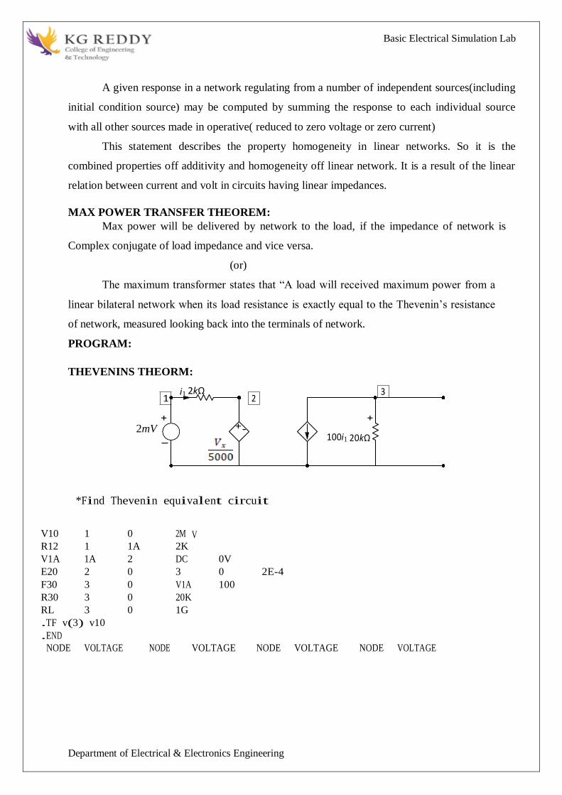
Basic Electrical Simulation Lab
Department of Electrical amp Electronics Engineering
i1 2kΩ
+
5000
+
minus minus
+
100i1 20kΩ
minus
1 3
2
A given response in a network regulating from a number of independent sources(including
initial condition source) may be computed by summing the response to each individual source
with all other sources made in operative( reduced to zero voltage or zero current)
This statement describes the property homogeneity in linear networks So it is the
combined properties off additivity and homogeneity off linear network It is a result of the linear
relation between current and volt in circuits having linear impedances
MAX POWER TRANSFER THEOREM
Max power will be delivered by network to the load if the impedance of network is
Complex conjugate of load impedance and vice versa
(or)
The maximum transformer states that ldquoA load will received maximum power from a
linear bilateral network when its load resistance is exactly equal to the Theveninrsquos resistance
of network measured looking back into the terminals of network
PROGRAM
THEVENINS THEORM
2mV -
Find Thevenin equivalent circuit
V10 1 0 2M V
R12 1 1A 2K
V1A 1A 2 DC 0V
E20 2 0 3 0 2E-4
F30 3 0 V1A 100
R30 3 0 20K
RL 3 0 1G
TF v(3) v10
END
NODE VOLTAGE NODE VOLTAGE NODE VOLTAGE NODE VOLTAGE
Basic Electrical Simulation Lab
Department of Electrical amp Electronics Engineering
NORTONS THEORM
PROGRAM
Vs 1 0 DC 20V
R1 1 2 18k
Rb 2 0 22k
Rc 2 3 33k
Is 3 0 RL
DC
end
MAXIMUM POWER TRANSFER THEOREM
PROGRAM
VS 1 0 DC 100
R1 1 2 10
R2 2 0 30
R3 1 3 20
R4 3 0 40
RL 2 3 RLOAD 1
MODEL RLOAD RES(R=25)
DC RES RLOAD(R) 0001 40 001
TF V(23) VS
PROBE
END
Basic Electrical Simulation Lab
Department of Electrical amp Electronics Engineering
SUPERPOSITION THEOREM
Program FOR CIRCUIT 1 FOR CIRCUIT 2
VDC 1 2 DC 10V VDC 1 2 DC 10V VDC 1 2 DC 0V
R1 1 3 100 R1 1 3 100 R1 1 3 100
R2 3 4 200 R2 3 4 200 R2 3 4 200
R3 3 6 470 R3 3 6 470 R3 3 6 470
R4 2 0 560 R4 2 0 560 R4 2 0 560
R5 4 5 100 R5 4 0 100 R5 4 5 100
VX 5 0 DC 10V VY 6 0 DC 0V VY 6 0 DC 0V
VY 6 0 DC 0V OP OP
OP END END
END
OUTPUT-
RESULT-
Basic Electrical Simulation Lab
Department of Electrical amp Electronics Engineering
EXPERIMET-6
WAVEFORM SYNTHESIS USING LAPLACE TRANSFORM
AIM To perform waveform synthesis using Laplace Transforms of a given signal
APPARATUS
1 OCTAVE
2 LINUX
THEORY
Bilateral Laplace transform
When one says the Laplace transform without qualification the unilateral or one-sided
transform is normally intended The Laplace transform can be alternatively defined as the bilateral
Laplace transform or two-sided Laplace transform by extending the limits of integration to be the
entire real axis If that is done the common unilateral transform simply becomes a special case of
the bilateral transform where the definition of the function being transformed is multiplied by the
Heaviside step function The bilateral Laplace transform is defined as follows
Inverse Laplace transform
The inverse Laplace transform is given by the following complex integral which is known by
various names (the Bromwich integral the Fourier-Mellin integral and Mellins inverse formula)
Example
Let y(t)=exp(t)
We have
The integral converges if sgt1 The functions exp(t) and 1(s-1) are partner functions
Basic Electrical Simulation Lab
Department of Electrical amp Electronics Engineering
PROGRAM-
Laplace Transform
clc
clear all
close all
syms t
x=exp(-2t)heaviside(t)
y=laplace(x)
disp(Laplace Transform of input signal)
y
z=ilaplace(y)
disp(Inverse Laplace Transform of input signal)
z
PROCEDURE-
1 Open OCTAVE
2 Open new script
3 Type the program
4 Save in current directory
5 Compile and Run the program
6 For the output see command window Figure window
OUTPUT-
RESULT-
Basic Electrical Simulation Lab
Department of Electrical amp Electronics Engineering
EXPERIMENT-7
LOCATING THE ZEROS AND POLES AND PLOTTING THE
POLE ZERO MAPS IN S-PLANE AND Z-PLANE FOR THE GIVEN
TRANSFER FUNCTION
AIM To locating the zeros and poles and plotting the pole zero maps in s-plane and z-plane
for the given transfer function
APPARATUS
1 OCTAVE
2 LINUX
THEORY
A Transfer Function is the ratio of the output of a system to the input of a system in the Laplace
domain considering its initial conditions to be zero If we have an input function of X(s) and an
output function Y(s) we define the transfer function H(s) to be
transfer function is the Laplace transform of a system‟ s impulse response
Given a continuous-time transfer function in the Laplace domain H(s) or a discrete-time one in
the Z-domain H(z) a zero is any value of s or z such that the transfer function is zero and a pole
is any value of s or z such that the transfer function is infinite
Zeros1 The value(s) for z where the numerator of the transfer function equals zero 2 The
complex frequencies that make the overall gain of the filter transfer function zero
Poles 1 The value(s) for z where the denominator of the transfer function equals zero 2 The
omplex frequencies that make the overall gain of the filter transfer function
infinite
Z-transforms
the Z-transform converts a discrete time-domain signal which is a sequence of real or complex
numbers into a complex frequency-domain representationThe Z-transform like many other
integral transforms can be defined as either a one-sided or two-sided transform
Basic Electrical Simulation Lab
Department of Electrical amp Electronics Engineering
Bilateral Z-transform
The bilateral or two-sided Z-transform of a discrete-time signal x[n] is the function X(z)
defined as
Unilateral Z-transform
Alternatively in cases where x[n] is defined only for n ge 0 the single-sided or unilateral
Z-transform is defined as
In signal processing this definition is used when the signal is causal
The roots of the equation P(z) = 0 correspond to the zeros of X(z)
The roots of the equation Q(z) = 0 correspond to the poles of X(z)
PROGRAM-
locating poles of zero on s-plane
clc
clear all
close all
num=input(enter numerator co-efficients)
den=input(enter denominator co-efficients)
h=tf(numden)
poles=roots(den)
zeros=roots(num)
sgrid
pzmap(h)
grid on
title(locating poles of zeros on s-plane)
Basic Electrical Simulation Lab
Department of Electrical amp Electronics Engineering
locating poles ampzeros on z-plane
clc
clear all
close all
num=input(enter numerator coefficient)
den=input(enter denominator coefficient)
p=roots(den)
z=roots(num)
zplane(pz)
grid
title(locating poler and zeros on s-plane)
PROCEDURE-
1 Open OCTAVE
2 Open new script
3 Type the program
4 Save in current directory
5 Compile and Run the program
6 For the output see command window Figure window
OUTPUT-
RESULT-
Basic Electrical Simulation Lab
Department of Electrical amp Electronics Engineering
EXPERIMENT-8
SIMULATION OF DC CIRCUITS
AIM To Simulate the DC network using PSPICE
APPARATUS
1 NGSPICE
2 LINUX
THEORY
Generally speaking network analysis is any structured technique used to mathematically
analyze a circuit (a ldquonetworkrdquo of interconnected components) Quite often the technician or
engineer will encounter circuits containing multiple sources of power or component
configurations which defy simplification by seriesparallel analysis techniques In those cases he
or she will be forced to use other means This chapter presents a few techniques useful in
analyzing such complex circuits
To analyse the above circuit one would first find the equivalent of R2 and R3 in parallel
then add R1 in series to arrive at a total resistance Then taking the voltage of battery B1 with
that total circuit resistance the total current could be calculated through the use of Ohmrsquos
Law (I=ER) then that current figure used to calculate voltage drops in the circuit All in all a
fairly simple procedure However the addition of just one more battery could change all of that
PROGRAM
Basic Electrical Simulation Lab
Department of Electrical amp Electronics Engineering
Vs 1 0 DC 20V
Ra 1 2 5k
Rb 2 0 4k
Rc 3 0 1k
Is 3 2 DC 20mA
DC
end
OUTPUT-
RESULT-
Basic Electrical Simulation Lab
Department of Electrical amp Electronics Engineering
EXPERIMENT-9
TRANSIENT ANALYSIS
AIM To find out the transient response by simulation of RLC circuits Using NGSPICE
APPARATUS
1 NGSPICE
2 LINUX
THEORY
The transient simulation is the calculation of a networks response on arbitrary excitations The
results are network quantities (branch currents and node voltages) as a function of time
Substantial for the transient analysis is the consideration of energy storing components ie
inductors and capacitorsThe relations between current and voltage of ideal capacitors and
inductors are given by
(61)
Or in terms of differential equations
(62)
To calculate these quantities in a computer program numerical integration methods are required
With the current-voltage relations of these components at hand it is possible to apply the modified
nodal analysis algorithm in order to calculate the networks response This means the transient
analysis attempts to find an approximation to the analytical solution at discrete time points using
numeric integration
CIRCUIT DIAGRAM
Basic Electrical Simulation Lab
Department of Electrical amp Electronics Engineering
PROGRAM
VIN1 1 0 PWL(0 0 1NS 1V 1MS 1V)
VIN2 4 0 PWL(0 0 1NS 1V 1MS 1V)
VIN3 7 0 PWL(0 0 1NS 1V 1MS 1V)
R1 1 2 2
R2 4 5 1
R3 7 8 8
L1 2 3 50UH
L2 5 6 50UH
L3 8 9 50UH
C1 3 0 10UF
C2 6 0 10UF
C3 9 0 10UF
TRAN 1US 400US
PLOT TRAN V(3) V(6) V(9)
PROBE
END
OUTPUT-
RESULT-
Basic Electrical Simulation Lab
Department of Electrical amp Electronics Engineering
EXPERIMENT-10
SIMULATION OF SINGLE PHASE DIODE BRIDGE RECTIFIERS WITH FILTER FOR
R amp RL LOAD
AIM To analyze the simulation of 1-Oslash diode bridge rectifiers with filter for R amp RL load using
NGSPICE
APPARATUS
1 NGSPICE
2 LINUX
THEORY
A bridge rectifier circuit is a common part of the electronic power supplies
Many electronic circuits require rectified DC power supply for powering the various electronic
basic components from available AC mains supply We can find this rectifier in a wide variety of
electronic AC power devices like home appliances motor controllers modulation process
welding applications etc
A Bridge rectifier is an Alternating Current (AC) to Direct Current (DC) converter that
rectifies mains AC input to DC output Bridge Rectifiers are widely used in power supplies that
provide necessary DC voltage for the electronic components or devices They can be constructed
with four or more diodes or any other controlled solid state switches Depending on the load
current requirements a proper bridge rectifier is selected Componentsrsquo ratings and specifications
breakdown voltage temperature ranges transient current rating forward current rating mounting
requirements and other considerations are taken into account while selecting a rectifier power
supply for an appropriate electronic circuitrsquos application
Bride rectifiers are classified into several types based on these factors type of supply
controlling capability bride circuitrsquos configurations etc Bridge rectifiers are mainly classified
into single and three phase rectifiers Both these types are further classified into uncontrolled half
controlled and full controlled rectifiers
Basic Electrical Simulation Lab
Department of Electrical amp Electronics Engineering
Program
VS 1 0 SIN(0 1697V 60HZ)
DF 5 4 DMOD
R1 4 7 10
L1 7 8 20MH
C1 4 6 793UF
RX 6 5 01
VX 8 5 DC 10V
VY 2 1 DC 0V
D1 2 4 DMOD
D2 5 3 DMOD
D3 3 4 DMOD
D4 5 2 DMOD
MODEL DMOD D( IS=22E-15 BV=1800 TT=0)
TRAN 10US 100MS 166MS
PROBE
FOUR 120HZ I(VX)
END
OUTPUT-
RESULT-
Basic Electrical Simulation Lab
Department of Electrical amp Electronics Engineering
EXPERIMENT-11
SIMULATION OF THREE PHASE DIODE BRIDGE RECTIFIERS WITH R RL LOAD
AIM To analyze the simulation of 3-Oslash diode bridge rectifiers with filter for R amp RL load using
NGSPICE
APPARATUS
1 NGSPICE
2 LINUX
THEORY
Three phase half controlled bridge converters amp fully controlled bridge converters are used
extensively in industrial applications up to about 15kW of output power The Three phase
controlled rectifiers provide a maximum dc output of
vdc(max)=2vm prod
The output ripple frequency is equal to the twice the ac supply frequency The single phase
full wave controlled rectifiers provide two output pulses during every input supply cycle
and hence are referred to as two pulse converters
Three phase converters are 3-phase controlled rectifiers which are used to convert ac input
power supply into dc output power across the load
Features of 3-phase controlled rectifiers are
Operate from 3 phase ac supply voltage
They provide higher dc output voltage and higher dc output power
Higher output voltage ripple frequency
Filtering requirements are simplified for smoothing out load voltage and load
current
Three phase controlled rectifiers are extensively used in high power variable speed
industrial dc drives
Basic Electrical Simulation Lab
Department of Electrical amp Electronics Engineering
Program
VAN 1 0 SIN(0V 200V 50HZ 0 0 0)
VBN 2 0 SIN(0V 200V 50HZ 0 0 -120)
VCN 3 0 SIN(0V 200V 50HZ 0 0 -240)
R 7 9 20
L 9 10 55MH
VX 10 8 DC 0V
VY 1 4 DC 0V
D1 4 7 DMOD
D2 8 2 DMOD
D3 3 7 DMOD
D4 8 4 DMOD
D5 2 7 DMOD
D6 8 3 DMOD
MODEL DMOD D(IS=22E-15 BV=1800V TT=0)
TRAN 5US 50MS 2166MS
PROBE
END
OUTPUT-
RESULT-
Basic Electrical Simulation Lab
Department of Electrical amp Electronics Engineering
EXPERIMENT-12
DESIGN OF LOW PASS AND HIGH PASS FILTERS
AIM To analyze the simulation of 3-Oslash diode bridge rectifiers with filter for R amp RL load using
NGSPICE
APPARATUS
1 OCTAVE
2 LINUX
THEORY
A filter is a circuit that has designed to pass a specified band of frequencies while attenuating all
signals outside this band Active filters employ transistors or op-amps plus resistors inductors
and capacitors There are four types of filters low-pass high-pass band-pass and band-
elimination (also referred to as band-reject or notch) filters Figure 71 illustrates frequency-
response plot for the four types of filters A low-pass filter is a circuit that has a constant output
voltage from dc up to a cutoff frequency fc As the frequency increases above fc the output
voltage is attenuated (decreases) Figure 71(a) is a plot of magnitude of the output voltage of a
low-pass filter versus frequency The range of frequencies that are transmitted is known as the
pass-band The range of frequencies that are attenuated is known as the stop-band The cutoff
frequency fc is also called the 0707 frequency the 3-dB frequency the corner frequency or the
break frequency High-pass filters attenuate the output voltage for all frequencies below the cutoff
frequency fc Above fc the magnitude of the output voltage is constant Figure 71(b) is the plot
for ideal and practical high-pass filters Band-pass filters pass only a band of frequencies while
attenuating all frequencies outside the band Band-elimination filters perform in an exactly
opposite way that is band-elimination filters reject a specified band of frequencies while passing
all frequencies outside the band Typical frequency-response plots for band-pass and band-
elimination filters are shown in Figure 71(c) and (d) In many filter applications it is necessary
for the closed-loop gain to be as close to 1 as possible within the pass band The Butterworth filter
is best suited for this type of application The Butterworth filter is also called a maximally flat or
flat-flat filter and all filter in this experiment will be of the Butterworth type Figure 72 shows
the ideal and the practical frequency response for three types of Butterworth filters As the roll-
offs become steeper they approach the ideal filter more closely
Basic Electrical Simulation Lab
Department of Electrical amp Electronics Engineering
PROGRAM
LOW PASS FILTER
N = 100 FIR filter order
Fp = 20e3 20 kHz passband-edge frequency
Fs = 96e3 96 kHz sampling frequency
Rp = 000057565 Corresponds to 001 dB peak-to-peak ripple
Rst = 1e-4 Corresponds to 80 dB stopband attenuation
eqnum = firceqrip(NFp(Fs2)[Rp Rst]passedge) eqnum = vec of coeffs
fvtool(eqnumFsFsColorWhite) Visualize filter
HIGH PASS FILTER
Fstop = 350
Fpass = 400
Astop = 65
Apass = 05
Fs = 1e3
d = designfilt(highpassfirStopbandFrequencyFstop
PassbandFrequencyFpassStopbandAttenuationAstop
PassbandRippleApassSampleRateFsDesignMethodequiripple)
fvtool(d)
OUTPUT-
RESULT-
Basic Electrical Simulation Lab
Department of Electrical amp Electronics Engineering
EXPERIMENT-13
FINDING THE EVEN AND ODD PARTS OF SIGNAL SEQUENCE AND REAL AND
IMAGINARY PARTS OF SIGNAL
AIM
program for finding even and odd parts of sequences Using OCTAVE Softwareamp
program for finding real and imaginary parts of sequences Using OCTAVE Software
APPARATUS
1 OCTAVE
2 LINUX
THEORY
Even and Odd Signal
One of characteristics of signal is symmetry that may be useful for signal analysis Even signals
are symmetric around vertical axis and Odd signals are symmetric about origin
Even Signal A signal is referred to as an even if it is identical to its time-reversed counterparts
x(t) = x(-t)
Odd Signal A signal is odd if x(t) = -x(-t)
An odd signal must be 0 at t=0 in other words odd signal passes the origin
Using the definition of even and odd signal any signal may be decomposed into a sum of its even
part xe(t) and its odd part xo(t) as follows
x(t)=xe(t)+xo(t)
x(t)=12x(t)+x(-t) +12x(t)-x(-t)
where
xe(t)=12x(t)+x(-t) ampxo(t)=12x(t)-x(-t)
It is an important fact because it is relative concept of Fourier series In Fourier series aperiodic
signal can be broken into a sum of sine and cosine signals Notice that sine function is odd signal
and cosine function is even signal
ENERGY AND POWER SIGNAL
A signal can be categorized into energy signal or power
signal An energy signal has a finite energy 0 lt E lt 1049279 In other words energy signals have
values only in the limited time duration For example a signal having only one square pulse is
energy signal A signal that decays exponentially has finite energy so it is also an energy signal
The power of an energy signal is 0 because of dividing finite energy by infinite time (or length)
If x(t) is a real-valued signal with Fourier transform X(f) and u(f) is the Heaviside step function
Basic Electrical Simulation Lab
Department of Electrical amp Electronics Engineering
then the function
contains only the non-negative frequency components of X(f) And the operation is reversible due
to the Hermitian property of X(f)
X(f) denotes the complex conjugate of X(f)
The inverse Fourier transform of Xa(f) is the analytic signal
where x^(t) is the Hilbert transform of x(t) and J is the imaginary unit
Basic Electrical Simulation Lab
Department of Electrical amp Electronics Engineering
PROGRAM-
Evenoddrealimaginary parts of a sequences
clc
clear all
close all
h=input(enter noof samples)
m=(h-1)2
n=-mm
x=input(enter sample values)
subplot(411)
stem(nxg)
xlabel(time)
ylabel(amplitude)
title(original sequence)
xmir=fliplr(x)
subplot(412)
stem(nxmirr)
xlabel(time)
ylabel(amplitude)
title(folded sequence)
even part of sequence
xeven=(x+xmir)2
subplot(413)
stem(nxevenr)
xlabel(time)
ylabel(amplitude)
title(even part of sequence)
odd part of sequence
xodd=(x-xmir)2
subplot(414)
stem(nxoddg)
xlabel(time)
ylabel(amplitude)
title(odd part of sequence)
Basic Electrical Simulation Lab
Department of Electrical amp Electronics Engineering
RealampImaginary parts of a sequences
clc
clear all
close all
y=input(enter complex numbers)
yreal=real(y)
disp(real values of y)
yreal
yimag=imag(y)
disp(imaginary values of y)
yimag
PROCEDURE-
1 Open OCTAVE
2 Open new script
3 Type the program
4 Save in current directory
5 Compile and Run the program
6 For the output see command window Figure window
OUTPUT-
RESULT-
Basic Electrical Simulation Lab
Department of Electrical amp Electronics Engineering
EXPERIMENT-14
FINDING THE FOURIER TRANSFORM OF A GIVEN SIGNAL AND PLOTTING ITS
MAGNITUDE AND PHASE SPECTRUM
AIM
Program for finding the fourier transform of a given signal Using OCTAVE Software amp Plotting
Its Magnitude And Phase Spectrum Using OCTAVE Software
APPARATUS
1 OCTAVE
2 LINUX
THEORY
The Fourier transform (FT) decomposes a function of time (a signal) into the
frequencies that make it up in a way similar to how a musical chord can be expressed as the
frequencies (or pitches) of its constituent notes The Fourier transform of a function of time itself
is a complex-valued function of frequency whose absolute value represents the amount of that
frequency present in the original function and whose complex argument is the phase offset of the
basic sinusoid in that frequency The Fourier transform is called the frequency domain
representation of the original signal The term Fourier transform refers to both the frequency
domain representation and the mathematical operation that associates the frequency domain
representation to a function of time The Fourier transform is not limited to functions of time but
in order to have a unified language the domain of the original function is commonly referred to as
the time domain For many functions of practical interest one can define an operation that
reverses this the inverse Fourier transformation also called Fourier synthesis of a frequency
domain representation combines the contributions of all the different frequencies to recover the
original function of time
Linear operations performed in one domain (time or frequency) have corresponding
operations in the other domain which are sometimes easier to perform The operation
of differentiation in the time domain corresponds to multiplication by the frequency[remark 1] so
some differential equations are easier to analyze in the frequency domain Also convolution in the
time domain corresponds to ordinary multiplication in the frequency domain Concretely this
means that any linear time-invariant system such as a filter applied to a signal can be expressed
relatively simply as an operation on frequencies After performing the desired operations
transformation of the result can be made back to the time domain Harmonic analysis is the
systematic study of the relationship between the frequency and time domains including the kinds
Basic Electrical Simulation Lab
Department of Electrical amp Electronics Engineering
of functions or operations that are simpler in one or the other and has deep connections to many
areas of modern mathematics
PROGRAM
Fs = 1000 Sampling frequency
T = 1Fs Sampling period
L = 1500 Length of signal
t = (0L-1)T Time vector
S = 07sin(2pi50t) + sin(2pi120t)
X = S + 2randn(size(t))
plot(1000t(150)X(150))
title(Signal Corrupted with Zero-Mean Random Noise)
xlabel(t (milliseconds))
ylabel(X(t))
Y = fft(X)
P2 = abs(YL)
P1 = P2(1L2+1)
P1(2end-1) = 2P1(2end-1)
f = Fs(0(L2))L
plot(fP1)
title(Single-Sided Amplitude Spectrum of X(t))
xlabel(f (Hz))
ylabel(|P1(f)|)
Y = fft(S)
P2 = abs(YL)
P1 = P2(1L2+1)
P1(2end-1) = 2P1(2end-1)
plot(fP1)
title(Single-Sided Amplitude Spectrum of S(t))
xlabel(f (Hz))
ylabel(|P1(f)|)
OUTPUT-
RESULT-
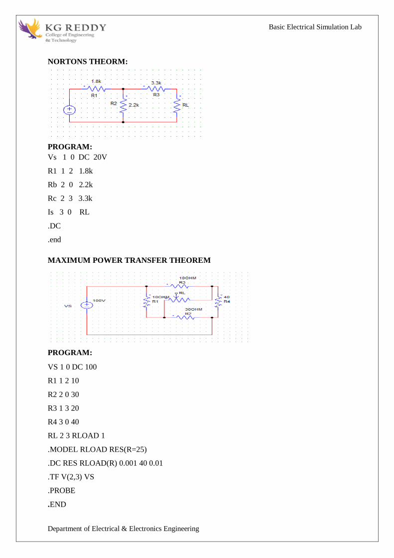
Basic Electrical Simulation Lab
Department of Electrical amp Electronics Engineering
NORTONS THEORM
PROGRAM
Vs 1 0 DC 20V
R1 1 2 18k
Rb 2 0 22k
Rc 2 3 33k
Is 3 0 RL
DC
end
MAXIMUM POWER TRANSFER THEOREM
PROGRAM
VS 1 0 DC 100
R1 1 2 10
R2 2 0 30
R3 1 3 20
R4 3 0 40
RL 2 3 RLOAD 1
MODEL RLOAD RES(R=25)
DC RES RLOAD(R) 0001 40 001
TF V(23) VS
PROBE
END
Basic Electrical Simulation Lab
Department of Electrical amp Electronics Engineering
SUPERPOSITION THEOREM
Program FOR CIRCUIT 1 FOR CIRCUIT 2
VDC 1 2 DC 10V VDC 1 2 DC 10V VDC 1 2 DC 0V
R1 1 3 100 R1 1 3 100 R1 1 3 100
R2 3 4 200 R2 3 4 200 R2 3 4 200
R3 3 6 470 R3 3 6 470 R3 3 6 470
R4 2 0 560 R4 2 0 560 R4 2 0 560
R5 4 5 100 R5 4 0 100 R5 4 5 100
VX 5 0 DC 10V VY 6 0 DC 0V VY 6 0 DC 0V
VY 6 0 DC 0V OP OP
OP END END
END
OUTPUT-
RESULT-
Basic Electrical Simulation Lab
Department of Electrical amp Electronics Engineering
EXPERIMET-6
WAVEFORM SYNTHESIS USING LAPLACE TRANSFORM
AIM To perform waveform synthesis using Laplace Transforms of a given signal
APPARATUS
1 OCTAVE
2 LINUX
THEORY
Bilateral Laplace transform
When one says the Laplace transform without qualification the unilateral or one-sided
transform is normally intended The Laplace transform can be alternatively defined as the bilateral
Laplace transform or two-sided Laplace transform by extending the limits of integration to be the
entire real axis If that is done the common unilateral transform simply becomes a special case of
the bilateral transform where the definition of the function being transformed is multiplied by the
Heaviside step function The bilateral Laplace transform is defined as follows
Inverse Laplace transform
The inverse Laplace transform is given by the following complex integral which is known by
various names (the Bromwich integral the Fourier-Mellin integral and Mellins inverse formula)
Example
Let y(t)=exp(t)
We have
The integral converges if sgt1 The functions exp(t) and 1(s-1) are partner functions
Basic Electrical Simulation Lab
Department of Electrical amp Electronics Engineering
PROGRAM-
Laplace Transform
clc
clear all
close all
syms t
x=exp(-2t)heaviside(t)
y=laplace(x)
disp(Laplace Transform of input signal)
y
z=ilaplace(y)
disp(Inverse Laplace Transform of input signal)
z
PROCEDURE-
1 Open OCTAVE
2 Open new script
3 Type the program
4 Save in current directory
5 Compile and Run the program
6 For the output see command window Figure window
OUTPUT-
RESULT-
Basic Electrical Simulation Lab
Department of Electrical amp Electronics Engineering
EXPERIMENT-7
LOCATING THE ZEROS AND POLES AND PLOTTING THE
POLE ZERO MAPS IN S-PLANE AND Z-PLANE FOR THE GIVEN
TRANSFER FUNCTION
AIM To locating the zeros and poles and plotting the pole zero maps in s-plane and z-plane
for the given transfer function
APPARATUS
1 OCTAVE
2 LINUX
THEORY
A Transfer Function is the ratio of the output of a system to the input of a system in the Laplace
domain considering its initial conditions to be zero If we have an input function of X(s) and an
output function Y(s) we define the transfer function H(s) to be
transfer function is the Laplace transform of a system‟ s impulse response
Given a continuous-time transfer function in the Laplace domain H(s) or a discrete-time one in
the Z-domain H(z) a zero is any value of s or z such that the transfer function is zero and a pole
is any value of s or z such that the transfer function is infinite
Zeros1 The value(s) for z where the numerator of the transfer function equals zero 2 The
complex frequencies that make the overall gain of the filter transfer function zero
Poles 1 The value(s) for z where the denominator of the transfer function equals zero 2 The
omplex frequencies that make the overall gain of the filter transfer function
infinite
Z-transforms
the Z-transform converts a discrete time-domain signal which is a sequence of real or complex
numbers into a complex frequency-domain representationThe Z-transform like many other
integral transforms can be defined as either a one-sided or two-sided transform
Basic Electrical Simulation Lab
Department of Electrical amp Electronics Engineering
Bilateral Z-transform
The bilateral or two-sided Z-transform of a discrete-time signal x[n] is the function X(z)
defined as
Unilateral Z-transform
Alternatively in cases where x[n] is defined only for n ge 0 the single-sided or unilateral
Z-transform is defined as
In signal processing this definition is used when the signal is causal
The roots of the equation P(z) = 0 correspond to the zeros of X(z)
The roots of the equation Q(z) = 0 correspond to the poles of X(z)
PROGRAM-
locating poles of zero on s-plane
clc
clear all
close all
num=input(enter numerator co-efficients)
den=input(enter denominator co-efficients)
h=tf(numden)
poles=roots(den)
zeros=roots(num)
sgrid
pzmap(h)
grid on
title(locating poles of zeros on s-plane)
Basic Electrical Simulation Lab
Department of Electrical amp Electronics Engineering
locating poles ampzeros on z-plane
clc
clear all
close all
num=input(enter numerator coefficient)
den=input(enter denominator coefficient)
p=roots(den)
z=roots(num)
zplane(pz)
grid
title(locating poler and zeros on s-plane)
PROCEDURE-
1 Open OCTAVE
2 Open new script
3 Type the program
4 Save in current directory
5 Compile and Run the program
6 For the output see command window Figure window
OUTPUT-
RESULT-
Basic Electrical Simulation Lab
Department of Electrical amp Electronics Engineering
EXPERIMENT-8
SIMULATION OF DC CIRCUITS
AIM To Simulate the DC network using PSPICE
APPARATUS
1 NGSPICE
2 LINUX
THEORY
Generally speaking network analysis is any structured technique used to mathematically
analyze a circuit (a ldquonetworkrdquo of interconnected components) Quite often the technician or
engineer will encounter circuits containing multiple sources of power or component
configurations which defy simplification by seriesparallel analysis techniques In those cases he
or she will be forced to use other means This chapter presents a few techniques useful in
analyzing such complex circuits
To analyse the above circuit one would first find the equivalent of R2 and R3 in parallel
then add R1 in series to arrive at a total resistance Then taking the voltage of battery B1 with
that total circuit resistance the total current could be calculated through the use of Ohmrsquos
Law (I=ER) then that current figure used to calculate voltage drops in the circuit All in all a
fairly simple procedure However the addition of just one more battery could change all of that
PROGRAM
Basic Electrical Simulation Lab
Department of Electrical amp Electronics Engineering
Vs 1 0 DC 20V
Ra 1 2 5k
Rb 2 0 4k
Rc 3 0 1k
Is 3 2 DC 20mA
DC
end
OUTPUT-
RESULT-
Basic Electrical Simulation Lab
Department of Electrical amp Electronics Engineering
EXPERIMENT-9
TRANSIENT ANALYSIS
AIM To find out the transient response by simulation of RLC circuits Using NGSPICE
APPARATUS
1 NGSPICE
2 LINUX
THEORY
The transient simulation is the calculation of a networks response on arbitrary excitations The
results are network quantities (branch currents and node voltages) as a function of time
Substantial for the transient analysis is the consideration of energy storing components ie
inductors and capacitorsThe relations between current and voltage of ideal capacitors and
inductors are given by
(61)
Or in terms of differential equations
(62)
To calculate these quantities in a computer program numerical integration methods are required
With the current-voltage relations of these components at hand it is possible to apply the modified
nodal analysis algorithm in order to calculate the networks response This means the transient
analysis attempts to find an approximation to the analytical solution at discrete time points using
numeric integration
CIRCUIT DIAGRAM
Basic Electrical Simulation Lab
Department of Electrical amp Electronics Engineering
PROGRAM
VIN1 1 0 PWL(0 0 1NS 1V 1MS 1V)
VIN2 4 0 PWL(0 0 1NS 1V 1MS 1V)
VIN3 7 0 PWL(0 0 1NS 1V 1MS 1V)
R1 1 2 2
R2 4 5 1
R3 7 8 8
L1 2 3 50UH
L2 5 6 50UH
L3 8 9 50UH
C1 3 0 10UF
C2 6 0 10UF
C3 9 0 10UF
TRAN 1US 400US
PLOT TRAN V(3) V(6) V(9)
PROBE
END
OUTPUT-
RESULT-
Basic Electrical Simulation Lab
Department of Electrical amp Electronics Engineering
EXPERIMENT-10
SIMULATION OF SINGLE PHASE DIODE BRIDGE RECTIFIERS WITH FILTER FOR
R amp RL LOAD
AIM To analyze the simulation of 1-Oslash diode bridge rectifiers with filter for R amp RL load using
NGSPICE
APPARATUS
1 NGSPICE
2 LINUX
THEORY
A bridge rectifier circuit is a common part of the electronic power supplies
Many electronic circuits require rectified DC power supply for powering the various electronic
basic components from available AC mains supply We can find this rectifier in a wide variety of
electronic AC power devices like home appliances motor controllers modulation process
welding applications etc
A Bridge rectifier is an Alternating Current (AC) to Direct Current (DC) converter that
rectifies mains AC input to DC output Bridge Rectifiers are widely used in power supplies that
provide necessary DC voltage for the electronic components or devices They can be constructed
with four or more diodes or any other controlled solid state switches Depending on the load
current requirements a proper bridge rectifier is selected Componentsrsquo ratings and specifications
breakdown voltage temperature ranges transient current rating forward current rating mounting
requirements and other considerations are taken into account while selecting a rectifier power
supply for an appropriate electronic circuitrsquos application
Bride rectifiers are classified into several types based on these factors type of supply
controlling capability bride circuitrsquos configurations etc Bridge rectifiers are mainly classified
into single and three phase rectifiers Both these types are further classified into uncontrolled half
controlled and full controlled rectifiers
Basic Electrical Simulation Lab
Department of Electrical amp Electronics Engineering
Program
VS 1 0 SIN(0 1697V 60HZ)
DF 5 4 DMOD
R1 4 7 10
L1 7 8 20MH
C1 4 6 793UF
RX 6 5 01
VX 8 5 DC 10V
VY 2 1 DC 0V
D1 2 4 DMOD
D2 5 3 DMOD
D3 3 4 DMOD
D4 5 2 DMOD
MODEL DMOD D( IS=22E-15 BV=1800 TT=0)
TRAN 10US 100MS 166MS
PROBE
FOUR 120HZ I(VX)
END
OUTPUT-
RESULT-
Basic Electrical Simulation Lab
Department of Electrical amp Electronics Engineering
EXPERIMENT-11
SIMULATION OF THREE PHASE DIODE BRIDGE RECTIFIERS WITH R RL LOAD
AIM To analyze the simulation of 3-Oslash diode bridge rectifiers with filter for R amp RL load using
NGSPICE
APPARATUS
1 NGSPICE
2 LINUX
THEORY
Three phase half controlled bridge converters amp fully controlled bridge converters are used
extensively in industrial applications up to about 15kW of output power The Three phase
controlled rectifiers provide a maximum dc output of
vdc(max)=2vm prod
The output ripple frequency is equal to the twice the ac supply frequency The single phase
full wave controlled rectifiers provide two output pulses during every input supply cycle
and hence are referred to as two pulse converters
Three phase converters are 3-phase controlled rectifiers which are used to convert ac input
power supply into dc output power across the load
Features of 3-phase controlled rectifiers are
Operate from 3 phase ac supply voltage
They provide higher dc output voltage and higher dc output power
Higher output voltage ripple frequency
Filtering requirements are simplified for smoothing out load voltage and load
current
Three phase controlled rectifiers are extensively used in high power variable speed
industrial dc drives
Basic Electrical Simulation Lab
Department of Electrical amp Electronics Engineering
Program
VAN 1 0 SIN(0V 200V 50HZ 0 0 0)
VBN 2 0 SIN(0V 200V 50HZ 0 0 -120)
VCN 3 0 SIN(0V 200V 50HZ 0 0 -240)
R 7 9 20
L 9 10 55MH
VX 10 8 DC 0V
VY 1 4 DC 0V
D1 4 7 DMOD
D2 8 2 DMOD
D3 3 7 DMOD
D4 8 4 DMOD
D5 2 7 DMOD
D6 8 3 DMOD
MODEL DMOD D(IS=22E-15 BV=1800V TT=0)
TRAN 5US 50MS 2166MS
PROBE
END
OUTPUT-
RESULT-
Basic Electrical Simulation Lab
Department of Electrical amp Electronics Engineering
EXPERIMENT-12
DESIGN OF LOW PASS AND HIGH PASS FILTERS
AIM To analyze the simulation of 3-Oslash diode bridge rectifiers with filter for R amp RL load using
NGSPICE
APPARATUS
1 OCTAVE
2 LINUX
THEORY
A filter is a circuit that has designed to pass a specified band of frequencies while attenuating all
signals outside this band Active filters employ transistors or op-amps plus resistors inductors
and capacitors There are four types of filters low-pass high-pass band-pass and band-
elimination (also referred to as band-reject or notch) filters Figure 71 illustrates frequency-
response plot for the four types of filters A low-pass filter is a circuit that has a constant output
voltage from dc up to a cutoff frequency fc As the frequency increases above fc the output
voltage is attenuated (decreases) Figure 71(a) is a plot of magnitude of the output voltage of a
low-pass filter versus frequency The range of frequencies that are transmitted is known as the
pass-band The range of frequencies that are attenuated is known as the stop-band The cutoff
frequency fc is also called the 0707 frequency the 3-dB frequency the corner frequency or the
break frequency High-pass filters attenuate the output voltage for all frequencies below the cutoff
frequency fc Above fc the magnitude of the output voltage is constant Figure 71(b) is the plot
for ideal and practical high-pass filters Band-pass filters pass only a band of frequencies while
attenuating all frequencies outside the band Band-elimination filters perform in an exactly
opposite way that is band-elimination filters reject a specified band of frequencies while passing
all frequencies outside the band Typical frequency-response plots for band-pass and band-
elimination filters are shown in Figure 71(c) and (d) In many filter applications it is necessary
for the closed-loop gain to be as close to 1 as possible within the pass band The Butterworth filter
is best suited for this type of application The Butterworth filter is also called a maximally flat or
flat-flat filter and all filter in this experiment will be of the Butterworth type Figure 72 shows
the ideal and the practical frequency response for three types of Butterworth filters As the roll-
offs become steeper they approach the ideal filter more closely
Basic Electrical Simulation Lab
Department of Electrical amp Electronics Engineering
PROGRAM
LOW PASS FILTER
N = 100 FIR filter order
Fp = 20e3 20 kHz passband-edge frequency
Fs = 96e3 96 kHz sampling frequency
Rp = 000057565 Corresponds to 001 dB peak-to-peak ripple
Rst = 1e-4 Corresponds to 80 dB stopband attenuation
eqnum = firceqrip(NFp(Fs2)[Rp Rst]passedge) eqnum = vec of coeffs
fvtool(eqnumFsFsColorWhite) Visualize filter
HIGH PASS FILTER
Fstop = 350
Fpass = 400
Astop = 65
Apass = 05
Fs = 1e3
d = designfilt(highpassfirStopbandFrequencyFstop
PassbandFrequencyFpassStopbandAttenuationAstop
PassbandRippleApassSampleRateFsDesignMethodequiripple)
fvtool(d)
OUTPUT-
RESULT-
Basic Electrical Simulation Lab
Department of Electrical amp Electronics Engineering
EXPERIMENT-13
FINDING THE EVEN AND ODD PARTS OF SIGNAL SEQUENCE AND REAL AND
IMAGINARY PARTS OF SIGNAL
AIM
program for finding even and odd parts of sequences Using OCTAVE Softwareamp
program for finding real and imaginary parts of sequences Using OCTAVE Software
APPARATUS
1 OCTAVE
2 LINUX
THEORY
Even and Odd Signal
One of characteristics of signal is symmetry that may be useful for signal analysis Even signals
are symmetric around vertical axis and Odd signals are symmetric about origin
Even Signal A signal is referred to as an even if it is identical to its time-reversed counterparts
x(t) = x(-t)
Odd Signal A signal is odd if x(t) = -x(-t)
An odd signal must be 0 at t=0 in other words odd signal passes the origin
Using the definition of even and odd signal any signal may be decomposed into a sum of its even
part xe(t) and its odd part xo(t) as follows
x(t)=xe(t)+xo(t)
x(t)=12x(t)+x(-t) +12x(t)-x(-t)
where
xe(t)=12x(t)+x(-t) ampxo(t)=12x(t)-x(-t)
It is an important fact because it is relative concept of Fourier series In Fourier series aperiodic
signal can be broken into a sum of sine and cosine signals Notice that sine function is odd signal
and cosine function is even signal
ENERGY AND POWER SIGNAL
A signal can be categorized into energy signal or power
signal An energy signal has a finite energy 0 lt E lt 1049279 In other words energy signals have
values only in the limited time duration For example a signal having only one square pulse is
energy signal A signal that decays exponentially has finite energy so it is also an energy signal
The power of an energy signal is 0 because of dividing finite energy by infinite time (or length)
If x(t) is a real-valued signal with Fourier transform X(f) and u(f) is the Heaviside step function
Basic Electrical Simulation Lab
Department of Electrical amp Electronics Engineering
then the function
contains only the non-negative frequency components of X(f) And the operation is reversible due
to the Hermitian property of X(f)
X(f) denotes the complex conjugate of X(f)
The inverse Fourier transform of Xa(f) is the analytic signal
where x^(t) is the Hilbert transform of x(t) and J is the imaginary unit
Basic Electrical Simulation Lab
Department of Electrical amp Electronics Engineering
PROGRAM-
Evenoddrealimaginary parts of a sequences
clc
clear all
close all
h=input(enter noof samples)
m=(h-1)2
n=-mm
x=input(enter sample values)
subplot(411)
stem(nxg)
xlabel(time)
ylabel(amplitude)
title(original sequence)
xmir=fliplr(x)
subplot(412)
stem(nxmirr)
xlabel(time)
ylabel(amplitude)
title(folded sequence)
even part of sequence
xeven=(x+xmir)2
subplot(413)
stem(nxevenr)
xlabel(time)
ylabel(amplitude)
title(even part of sequence)
odd part of sequence
xodd=(x-xmir)2
subplot(414)
stem(nxoddg)
xlabel(time)
ylabel(amplitude)
title(odd part of sequence)
Basic Electrical Simulation Lab
Department of Electrical amp Electronics Engineering
RealampImaginary parts of a sequences
clc
clear all
close all
y=input(enter complex numbers)
yreal=real(y)
disp(real values of y)
yreal
yimag=imag(y)
disp(imaginary values of y)
yimag
PROCEDURE-
1 Open OCTAVE
2 Open new script
3 Type the program
4 Save in current directory
5 Compile and Run the program
6 For the output see command window Figure window
OUTPUT-
RESULT-
Basic Electrical Simulation Lab
Department of Electrical amp Electronics Engineering
EXPERIMENT-14
FINDING THE FOURIER TRANSFORM OF A GIVEN SIGNAL AND PLOTTING ITS
MAGNITUDE AND PHASE SPECTRUM
AIM
Program for finding the fourier transform of a given signal Using OCTAVE Software amp Plotting
Its Magnitude And Phase Spectrum Using OCTAVE Software
APPARATUS
1 OCTAVE
2 LINUX
THEORY
The Fourier transform (FT) decomposes a function of time (a signal) into the
frequencies that make it up in a way similar to how a musical chord can be expressed as the
frequencies (or pitches) of its constituent notes The Fourier transform of a function of time itself
is a complex-valued function of frequency whose absolute value represents the amount of that
frequency present in the original function and whose complex argument is the phase offset of the
basic sinusoid in that frequency The Fourier transform is called the frequency domain
representation of the original signal The term Fourier transform refers to both the frequency
domain representation and the mathematical operation that associates the frequency domain
representation to a function of time The Fourier transform is not limited to functions of time but
in order to have a unified language the domain of the original function is commonly referred to as
the time domain For many functions of practical interest one can define an operation that
reverses this the inverse Fourier transformation also called Fourier synthesis of a frequency
domain representation combines the contributions of all the different frequencies to recover the
original function of time
Linear operations performed in one domain (time or frequency) have corresponding
operations in the other domain which are sometimes easier to perform The operation
of differentiation in the time domain corresponds to multiplication by the frequency[remark 1] so
some differential equations are easier to analyze in the frequency domain Also convolution in the
time domain corresponds to ordinary multiplication in the frequency domain Concretely this
means that any linear time-invariant system such as a filter applied to a signal can be expressed
relatively simply as an operation on frequencies After performing the desired operations
transformation of the result can be made back to the time domain Harmonic analysis is the
systematic study of the relationship between the frequency and time domains including the kinds
Basic Electrical Simulation Lab
Department of Electrical amp Electronics Engineering
of functions or operations that are simpler in one or the other and has deep connections to many
areas of modern mathematics
PROGRAM
Fs = 1000 Sampling frequency
T = 1Fs Sampling period
L = 1500 Length of signal
t = (0L-1)T Time vector
S = 07sin(2pi50t) + sin(2pi120t)
X = S + 2randn(size(t))
plot(1000t(150)X(150))
title(Signal Corrupted with Zero-Mean Random Noise)
xlabel(t (milliseconds))
ylabel(X(t))
Y = fft(X)
P2 = abs(YL)
P1 = P2(1L2+1)
P1(2end-1) = 2P1(2end-1)
f = Fs(0(L2))L
plot(fP1)
title(Single-Sided Amplitude Spectrum of X(t))
xlabel(f (Hz))
ylabel(|P1(f)|)
Y = fft(S)
P2 = abs(YL)
P1 = P2(1L2+1)
P1(2end-1) = 2P1(2end-1)
plot(fP1)
title(Single-Sided Amplitude Spectrum of S(t))
xlabel(f (Hz))
ylabel(|P1(f)|)
OUTPUT-
RESULT-
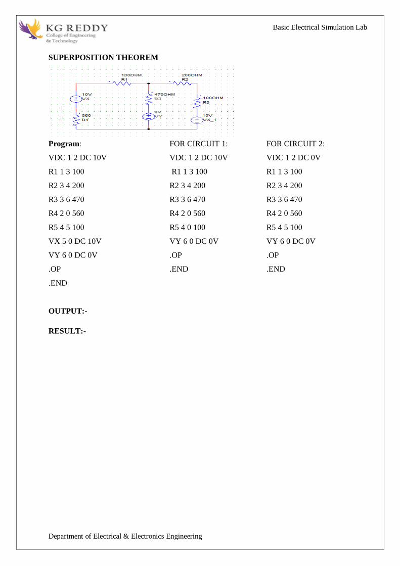
Basic Electrical Simulation Lab
Department of Electrical amp Electronics Engineering
PROGRAM-
Laplace Transform
clc
clear all
close all
syms t
x=exp(-2t)heaviside(t)
y=laplace(x)
disp(Laplace Transform of input signal)
y
z=ilaplace(y)
disp(Inverse Laplace Transform of input signal)
z
PROCEDURE-
1 Open OCTAVE
2 Open new script
3 Type the program
4 Save in current directory
5 Compile and Run the program
6 For the output see command window Figure window
OUTPUT-
RESULT-
Basic Electrical Simulation Lab
Department of Electrical amp Electronics Engineering
EXPERIMENT-7
LOCATING THE ZEROS AND POLES AND PLOTTING THE
POLE ZERO MAPS IN S-PLANE AND Z-PLANE FOR THE GIVEN
TRANSFER FUNCTION
AIM To locating the zeros and poles and plotting the pole zero maps in s-plane and z-plane
for the given transfer function
APPARATUS
1 OCTAVE
2 LINUX
THEORY
A Transfer Function is the ratio of the output of a system to the input of a system in the Laplace
domain considering its initial conditions to be zero If we have an input function of X(s) and an
output function Y(s) we define the transfer function H(s) to be
transfer function is the Laplace transform of a system‟ s impulse response
Given a continuous-time transfer function in the Laplace domain H(s) or a discrete-time one in
the Z-domain H(z) a zero is any value of s or z such that the transfer function is zero and a pole
is any value of s or z such that the transfer function is infinite
Zeros1 The value(s) for z where the numerator of the transfer function equals zero 2 The
complex frequencies that make the overall gain of the filter transfer function zero
Poles 1 The value(s) for z where the denominator of the transfer function equals zero 2 The
omplex frequencies that make the overall gain of the filter transfer function
infinite
Z-transforms
the Z-transform converts a discrete time-domain signal which is a sequence of real or complex
numbers into a complex frequency-domain representationThe Z-transform like many other
integral transforms can be defined as either a one-sided or two-sided transform
Basic Electrical Simulation Lab
Department of Electrical amp Electronics Engineering
Bilateral Z-transform
The bilateral or two-sided Z-transform of a discrete-time signal x[n] is the function X(z)
defined as
Unilateral Z-transform
Alternatively in cases where x[n] is defined only for n ge 0 the single-sided or unilateral
Z-transform is defined as
In signal processing this definition is used when the signal is causal
The roots of the equation P(z) = 0 correspond to the zeros of X(z)
The roots of the equation Q(z) = 0 correspond to the poles of X(z)
PROGRAM-
locating poles of zero on s-plane
clc
clear all
close all
num=input(enter numerator co-efficients)
den=input(enter denominator co-efficients)
h=tf(numden)
poles=roots(den)
zeros=roots(num)
sgrid
pzmap(h)
grid on
title(locating poles of zeros on s-plane)
Basic Electrical Simulation Lab
Department of Electrical amp Electronics Engineering
locating poles ampzeros on z-plane
clc
clear all
close all
num=input(enter numerator coefficient)
den=input(enter denominator coefficient)
p=roots(den)
z=roots(num)
zplane(pz)
grid
title(locating poler and zeros on s-plane)
PROCEDURE-
1 Open OCTAVE
2 Open new script
3 Type the program
4 Save in current directory
5 Compile and Run the program
6 For the output see command window Figure window
OUTPUT-
RESULT-
Basic Electrical Simulation Lab
Department of Electrical amp Electronics Engineering
EXPERIMENT-8
SIMULATION OF DC CIRCUITS
AIM To Simulate the DC network using PSPICE
APPARATUS
1 NGSPICE
2 LINUX
THEORY
Generally speaking network analysis is any structured technique used to mathematically
analyze a circuit (a ldquonetworkrdquo of interconnected components) Quite often the technician or
engineer will encounter circuits containing multiple sources of power or component
configurations which defy simplification by seriesparallel analysis techniques In those cases he
or she will be forced to use other means This chapter presents a few techniques useful in
analyzing such complex circuits
To analyse the above circuit one would first find the equivalent of R2 and R3 in parallel
then add R1 in series to arrive at a total resistance Then taking the voltage of battery B1 with
that total circuit resistance the total current could be calculated through the use of Ohmrsquos
Law (I=ER) then that current figure used to calculate voltage drops in the circuit All in all a
fairly simple procedure However the addition of just one more battery could change all of that
PROGRAM
Basic Electrical Simulation Lab
Department of Electrical amp Electronics Engineering
Vs 1 0 DC 20V
Ra 1 2 5k
Rb 2 0 4k
Rc 3 0 1k
Is 3 2 DC 20mA
DC
end
OUTPUT-
RESULT-
Basic Electrical Simulation Lab
Department of Electrical amp Electronics Engineering
EXPERIMENT-9
TRANSIENT ANALYSIS
AIM To find out the transient response by simulation of RLC circuits Using NGSPICE
APPARATUS
1 NGSPICE
2 LINUX
THEORY
The transient simulation is the calculation of a networks response on arbitrary excitations The
results are network quantities (branch currents and node voltages) as a function of time
Substantial for the transient analysis is the consideration of energy storing components ie
inductors and capacitorsThe relations between current and voltage of ideal capacitors and
inductors are given by
(61)
Or in terms of differential equations
(62)
To calculate these quantities in a computer program numerical integration methods are required
With the current-voltage relations of these components at hand it is possible to apply the modified
nodal analysis algorithm in order to calculate the networks response This means the transient
analysis attempts to find an approximation to the analytical solution at discrete time points using
numeric integration
CIRCUIT DIAGRAM
Basic Electrical Simulation Lab
Department of Electrical amp Electronics Engineering
PROGRAM
VIN1 1 0 PWL(0 0 1NS 1V 1MS 1V)
VIN2 4 0 PWL(0 0 1NS 1V 1MS 1V)
VIN3 7 0 PWL(0 0 1NS 1V 1MS 1V)
R1 1 2 2
R2 4 5 1
R3 7 8 8
L1 2 3 50UH
L2 5 6 50UH
L3 8 9 50UH
C1 3 0 10UF
C2 6 0 10UF
C3 9 0 10UF
TRAN 1US 400US
PLOT TRAN V(3) V(6) V(9)
PROBE
END
OUTPUT-
RESULT-
Basic Electrical Simulation Lab
Department of Electrical amp Electronics Engineering
EXPERIMENT-10
SIMULATION OF SINGLE PHASE DIODE BRIDGE RECTIFIERS WITH FILTER FOR
R amp RL LOAD
AIM To analyze the simulation of 1-Oslash diode bridge rectifiers with filter for R amp RL load using
NGSPICE
APPARATUS
1 NGSPICE
2 LINUX
THEORY
A bridge rectifier circuit is a common part of the electronic power supplies
Many electronic circuits require rectified DC power supply for powering the various electronic
basic components from available AC mains supply We can find this rectifier in a wide variety of
electronic AC power devices like home appliances motor controllers modulation process
welding applications etc
A Bridge rectifier is an Alternating Current (AC) to Direct Current (DC) converter that
rectifies mains AC input to DC output Bridge Rectifiers are widely used in power supplies that
provide necessary DC voltage for the electronic components or devices They can be constructed
with four or more diodes or any other controlled solid state switches Depending on the load
current requirements a proper bridge rectifier is selected Componentsrsquo ratings and specifications
breakdown voltage temperature ranges transient current rating forward current rating mounting
requirements and other considerations are taken into account while selecting a rectifier power
supply for an appropriate electronic circuitrsquos application
Bride rectifiers are classified into several types based on these factors type of supply
controlling capability bride circuitrsquos configurations etc Bridge rectifiers are mainly classified
into single and three phase rectifiers Both these types are further classified into uncontrolled half
controlled and full controlled rectifiers
Basic Electrical Simulation Lab
Department of Electrical amp Electronics Engineering
Program
VS 1 0 SIN(0 1697V 60HZ)
DF 5 4 DMOD
R1 4 7 10
L1 7 8 20MH
C1 4 6 793UF
RX 6 5 01
VX 8 5 DC 10V
VY 2 1 DC 0V
D1 2 4 DMOD
D2 5 3 DMOD
D3 3 4 DMOD
D4 5 2 DMOD
MODEL DMOD D( IS=22E-15 BV=1800 TT=0)
TRAN 10US 100MS 166MS
PROBE
FOUR 120HZ I(VX)
END
OUTPUT-
RESULT-
Basic Electrical Simulation Lab
Department of Electrical amp Electronics Engineering
EXPERIMENT-11
SIMULATION OF THREE PHASE DIODE BRIDGE RECTIFIERS WITH R RL LOAD
AIM To analyze the simulation of 3-Oslash diode bridge rectifiers with filter for R amp RL load using
NGSPICE
APPARATUS
1 NGSPICE
2 LINUX
THEORY
Three phase half controlled bridge converters amp fully controlled bridge converters are used
extensively in industrial applications up to about 15kW of output power The Three phase
controlled rectifiers provide a maximum dc output of
vdc(max)=2vm prod
The output ripple frequency is equal to the twice the ac supply frequency The single phase
full wave controlled rectifiers provide two output pulses during every input supply cycle
and hence are referred to as two pulse converters
Three phase converters are 3-phase controlled rectifiers which are used to convert ac input
power supply into dc output power across the load
Features of 3-phase controlled rectifiers are
Operate from 3 phase ac supply voltage
They provide higher dc output voltage and higher dc output power
Higher output voltage ripple frequency
Filtering requirements are simplified for smoothing out load voltage and load
current
Three phase controlled rectifiers are extensively used in high power variable speed
industrial dc drives
Basic Electrical Simulation Lab
Department of Electrical amp Electronics Engineering
Program
VAN 1 0 SIN(0V 200V 50HZ 0 0 0)
VBN 2 0 SIN(0V 200V 50HZ 0 0 -120)
VCN 3 0 SIN(0V 200V 50HZ 0 0 -240)
R 7 9 20
L 9 10 55MH
VX 10 8 DC 0V
VY 1 4 DC 0V
D1 4 7 DMOD
D2 8 2 DMOD
D3 3 7 DMOD
D4 8 4 DMOD
D5 2 7 DMOD
D6 8 3 DMOD
MODEL DMOD D(IS=22E-15 BV=1800V TT=0)
TRAN 5US 50MS 2166MS
PROBE
END
OUTPUT-
RESULT-
Basic Electrical Simulation Lab
Department of Electrical amp Electronics Engineering
EXPERIMENT-12
DESIGN OF LOW PASS AND HIGH PASS FILTERS
AIM To analyze the simulation of 3-Oslash diode bridge rectifiers with filter for R amp RL load using
NGSPICE
APPARATUS
1 OCTAVE
2 LINUX
THEORY
A filter is a circuit that has designed to pass a specified band of frequencies while attenuating all
signals outside this band Active filters employ transistors or op-amps plus resistors inductors
and capacitors There are four types of filters low-pass high-pass band-pass and band-
elimination (also referred to as band-reject or notch) filters Figure 71 illustrates frequency-
response plot for the four types of filters A low-pass filter is a circuit that has a constant output
voltage from dc up to a cutoff frequency fc As the frequency increases above fc the output
voltage is attenuated (decreases) Figure 71(a) is a plot of magnitude of the output voltage of a
low-pass filter versus frequency The range of frequencies that are transmitted is known as the
pass-band The range of frequencies that are attenuated is known as the stop-band The cutoff
frequency fc is also called the 0707 frequency the 3-dB frequency the corner frequency or the
break frequency High-pass filters attenuate the output voltage for all frequencies below the cutoff
frequency fc Above fc the magnitude of the output voltage is constant Figure 71(b) is the plot
for ideal and practical high-pass filters Band-pass filters pass only a band of frequencies while
attenuating all frequencies outside the band Band-elimination filters perform in an exactly
opposite way that is band-elimination filters reject a specified band of frequencies while passing
all frequencies outside the band Typical frequency-response plots for band-pass and band-
elimination filters are shown in Figure 71(c) and (d) In many filter applications it is necessary
for the closed-loop gain to be as close to 1 as possible within the pass band The Butterworth filter
is best suited for this type of application The Butterworth filter is also called a maximally flat or
flat-flat filter and all filter in this experiment will be of the Butterworth type Figure 72 shows
the ideal and the practical frequency response for three types of Butterworth filters As the roll-
offs become steeper they approach the ideal filter more closely
Basic Electrical Simulation Lab
Department of Electrical amp Electronics Engineering
PROGRAM
LOW PASS FILTER
N = 100 FIR filter order
Fp = 20e3 20 kHz passband-edge frequency
Fs = 96e3 96 kHz sampling frequency
Rp = 000057565 Corresponds to 001 dB peak-to-peak ripple
Rst = 1e-4 Corresponds to 80 dB stopband attenuation
eqnum = firceqrip(NFp(Fs2)[Rp Rst]passedge) eqnum = vec of coeffs
fvtool(eqnumFsFsColorWhite) Visualize filter
HIGH PASS FILTER
Fstop = 350
Fpass = 400
Astop = 65
Apass = 05
Fs = 1e3
d = designfilt(highpassfirStopbandFrequencyFstop
PassbandFrequencyFpassStopbandAttenuationAstop
PassbandRippleApassSampleRateFsDesignMethodequiripple)
fvtool(d)
OUTPUT-
RESULT-
Basic Electrical Simulation Lab
Department of Electrical amp Electronics Engineering
EXPERIMENT-13
FINDING THE EVEN AND ODD PARTS OF SIGNAL SEQUENCE AND REAL AND
IMAGINARY PARTS OF SIGNAL
AIM
program for finding even and odd parts of sequences Using OCTAVE Softwareamp
program for finding real and imaginary parts of sequences Using OCTAVE Software
APPARATUS
1 OCTAVE
2 LINUX
THEORY
Even and Odd Signal
One of characteristics of signal is symmetry that may be useful for signal analysis Even signals
are symmetric around vertical axis and Odd signals are symmetric about origin
Even Signal A signal is referred to as an even if it is identical to its time-reversed counterparts
x(t) = x(-t)
Odd Signal A signal is odd if x(t) = -x(-t)
An odd signal must be 0 at t=0 in other words odd signal passes the origin
Using the definition of even and odd signal any signal may be decomposed into a sum of its even
part xe(t) and its odd part xo(t) as follows
x(t)=xe(t)+xo(t)
x(t)=12x(t)+x(-t) +12x(t)-x(-t)
where
xe(t)=12x(t)+x(-t) ampxo(t)=12x(t)-x(-t)
It is an important fact because it is relative concept of Fourier series In Fourier series aperiodic
signal can be broken into a sum of sine and cosine signals Notice that sine function is odd signal
and cosine function is even signal
ENERGY AND POWER SIGNAL
A signal can be categorized into energy signal or power
signal An energy signal has a finite energy 0 lt E lt 1049279 In other words energy signals have
values only in the limited time duration For example a signal having only one square pulse is
energy signal A signal that decays exponentially has finite energy so it is also an energy signal
The power of an energy signal is 0 because of dividing finite energy by infinite time (or length)
If x(t) is a real-valued signal with Fourier transform X(f) and u(f) is the Heaviside step function
Basic Electrical Simulation Lab
Department of Electrical amp Electronics Engineering
then the function
contains only the non-negative frequency components of X(f) And the operation is reversible due
to the Hermitian property of X(f)
X(f) denotes the complex conjugate of X(f)
The inverse Fourier transform of Xa(f) is the analytic signal
where x^(t) is the Hilbert transform of x(t) and J is the imaginary unit
Basic Electrical Simulation Lab
Department of Electrical amp Electronics Engineering
PROGRAM-
Evenoddrealimaginary parts of a sequences
clc
clear all
close all
h=input(enter noof samples)
m=(h-1)2
n=-mm
x=input(enter sample values)
subplot(411)
stem(nxg)
xlabel(time)
ylabel(amplitude)
title(original sequence)
xmir=fliplr(x)
subplot(412)
stem(nxmirr)
xlabel(time)
ylabel(amplitude)
title(folded sequence)
even part of sequence
xeven=(x+xmir)2
subplot(413)
stem(nxevenr)
xlabel(time)
ylabel(amplitude)
title(even part of sequence)
odd part of sequence
xodd=(x-xmir)2
subplot(414)
stem(nxoddg)
xlabel(time)
ylabel(amplitude)
title(odd part of sequence)
Basic Electrical Simulation Lab
Department of Electrical amp Electronics Engineering
RealampImaginary parts of a sequences
clc
clear all
close all
y=input(enter complex numbers)
yreal=real(y)
disp(real values of y)
yreal
yimag=imag(y)
disp(imaginary values of y)
yimag
PROCEDURE-
1 Open OCTAVE
2 Open new script
3 Type the program
4 Save in current directory
5 Compile and Run the program
6 For the output see command window Figure window
OUTPUT-
RESULT-
Basic Electrical Simulation Lab
Department of Electrical amp Electronics Engineering
EXPERIMENT-14
FINDING THE FOURIER TRANSFORM OF A GIVEN SIGNAL AND PLOTTING ITS
MAGNITUDE AND PHASE SPECTRUM
AIM
Program for finding the fourier transform of a given signal Using OCTAVE Software amp Plotting
Its Magnitude And Phase Spectrum Using OCTAVE Software
APPARATUS
1 OCTAVE
2 LINUX
THEORY
The Fourier transform (FT) decomposes a function of time (a signal) into the
frequencies that make it up in a way similar to how a musical chord can be expressed as the
frequencies (or pitches) of its constituent notes The Fourier transform of a function of time itself
is a complex-valued function of frequency whose absolute value represents the amount of that
frequency present in the original function and whose complex argument is the phase offset of the
basic sinusoid in that frequency The Fourier transform is called the frequency domain
representation of the original signal The term Fourier transform refers to both the frequency
domain representation and the mathematical operation that associates the frequency domain
representation to a function of time The Fourier transform is not limited to functions of time but
in order to have a unified language the domain of the original function is commonly referred to as
the time domain For many functions of practical interest one can define an operation that
reverses this the inverse Fourier transformation also called Fourier synthesis of a frequency
domain representation combines the contributions of all the different frequencies to recover the
original function of time
Linear operations performed in one domain (time or frequency) have corresponding
operations in the other domain which are sometimes easier to perform The operation
of differentiation in the time domain corresponds to multiplication by the frequency[remark 1] so
some differential equations are easier to analyze in the frequency domain Also convolution in the
time domain corresponds to ordinary multiplication in the frequency domain Concretely this
means that any linear time-invariant system such as a filter applied to a signal can be expressed
relatively simply as an operation on frequencies After performing the desired operations
transformation of the result can be made back to the time domain Harmonic analysis is the
systematic study of the relationship between the frequency and time domains including the kinds
Basic Electrical Simulation Lab
Department of Electrical amp Electronics Engineering
of functions or operations that are simpler in one or the other and has deep connections to many
areas of modern mathematics
PROGRAM
Fs = 1000 Sampling frequency
T = 1Fs Sampling period
L = 1500 Length of signal
t = (0L-1)T Time vector
S = 07sin(2pi50t) + sin(2pi120t)
X = S + 2randn(size(t))
plot(1000t(150)X(150))
title(Signal Corrupted with Zero-Mean Random Noise)
xlabel(t (milliseconds))
ylabel(X(t))
Y = fft(X)
P2 = abs(YL)
P1 = P2(1L2+1)
P1(2end-1) = 2P1(2end-1)
f = Fs(0(L2))L
plot(fP1)
title(Single-Sided Amplitude Spectrum of X(t))
xlabel(f (Hz))
ylabel(|P1(f)|)
Y = fft(S)
P2 = abs(YL)
P1 = P2(1L2+1)
P1(2end-1) = 2P1(2end-1)
plot(fP1)
title(Single-Sided Amplitude Spectrum of S(t))
xlabel(f (Hz))
ylabel(|P1(f)|)
OUTPUT-
RESULT-
Basic Electrical Simulation Lab
Department of Electrical amp Electronics Engineering
Bilateral Z-transform
The bilateral or two-sided Z-transform of a discrete-time signal x[n] is the function X(z)
defined as
Unilateral Z-transform
Alternatively in cases where x[n] is defined only for n ge 0 the single-sided or unilateral
Z-transform is defined as
In signal processing this definition is used when the signal is causal
The roots of the equation P(z) = 0 correspond to the zeros of X(z)
The roots of the equation Q(z) = 0 correspond to the poles of X(z)
PROGRAM-
locating poles of zero on s-plane
clc
clear all
close all
num=input(enter numerator co-efficients)
den=input(enter denominator co-efficients)
h=tf(numden)
poles=roots(den)
zeros=roots(num)
sgrid
pzmap(h)
grid on
title(locating poles of zeros on s-plane)
Basic Electrical Simulation Lab
Department of Electrical amp Electronics Engineering
locating poles ampzeros on z-plane
clc
clear all
close all
num=input(enter numerator coefficient)
den=input(enter denominator coefficient)
p=roots(den)
z=roots(num)
zplane(pz)
grid
title(locating poler and zeros on s-plane)
PROCEDURE-
1 Open OCTAVE
2 Open new script
3 Type the program
4 Save in current directory
5 Compile and Run the program
6 For the output see command window Figure window
OUTPUT-
RESULT-
Basic Electrical Simulation Lab
Department of Electrical amp Electronics Engineering
EXPERIMENT-8
SIMULATION OF DC CIRCUITS
AIM To Simulate the DC network using PSPICE
APPARATUS
1 NGSPICE
2 LINUX
THEORY
Generally speaking network analysis is any structured technique used to mathematically
analyze a circuit (a ldquonetworkrdquo of interconnected components) Quite often the technician or
engineer will encounter circuits containing multiple sources of power or component
configurations which defy simplification by seriesparallel analysis techniques In those cases he
or she will be forced to use other means This chapter presents a few techniques useful in
analyzing such complex circuits
To analyse the above circuit one would first find the equivalent of R2 and R3 in parallel
then add R1 in series to arrive at a total resistance Then taking the voltage of battery B1 with
that total circuit resistance the total current could be calculated through the use of Ohmrsquos
Law (I=ER) then that current figure used to calculate voltage drops in the circuit All in all a
fairly simple procedure However the addition of just one more battery could change all of that
PROGRAM
Basic Electrical Simulation Lab
Department of Electrical amp Electronics Engineering
Vs 1 0 DC 20V
Ra 1 2 5k
Rb 2 0 4k
Rc 3 0 1k
Is 3 2 DC 20mA
DC
end
OUTPUT-
RESULT-
Basic Electrical Simulation Lab
Department of Electrical amp Electronics Engineering
EXPERIMENT-9
TRANSIENT ANALYSIS
AIM To find out the transient response by simulation of RLC circuits Using NGSPICE
APPARATUS
1 NGSPICE
2 LINUX
THEORY
The transient simulation is the calculation of a networks response on arbitrary excitations The
results are network quantities (branch currents and node voltages) as a function of time
Substantial for the transient analysis is the consideration of energy storing components ie
inductors and capacitorsThe relations between current and voltage of ideal capacitors and
inductors are given by
(61)
Or in terms of differential equations
(62)
To calculate these quantities in a computer program numerical integration methods are required
With the current-voltage relations of these components at hand it is possible to apply the modified
nodal analysis algorithm in order to calculate the networks response This means the transient
analysis attempts to find an approximation to the analytical solution at discrete time points using
numeric integration
CIRCUIT DIAGRAM
Basic Electrical Simulation Lab
Department of Electrical amp Electronics Engineering
PROGRAM
VIN1 1 0 PWL(0 0 1NS 1V 1MS 1V)
VIN2 4 0 PWL(0 0 1NS 1V 1MS 1V)
VIN3 7 0 PWL(0 0 1NS 1V 1MS 1V)
R1 1 2 2
R2 4 5 1
R3 7 8 8
L1 2 3 50UH
L2 5 6 50UH
L3 8 9 50UH
C1 3 0 10UF
C2 6 0 10UF
C3 9 0 10UF
TRAN 1US 400US
PLOT TRAN V(3) V(6) V(9)
PROBE
END
OUTPUT-
RESULT-
Basic Electrical Simulation Lab
Department of Electrical amp Electronics Engineering
EXPERIMENT-10
SIMULATION OF SINGLE PHASE DIODE BRIDGE RECTIFIERS WITH FILTER FOR
R amp RL LOAD
AIM To analyze the simulation of 1-Oslash diode bridge rectifiers with filter for R amp RL load using
NGSPICE
APPARATUS
1 NGSPICE
2 LINUX
THEORY
A bridge rectifier circuit is a common part of the electronic power supplies
Many electronic circuits require rectified DC power supply for powering the various electronic
basic components from available AC mains supply We can find this rectifier in a wide variety of
electronic AC power devices like home appliances motor controllers modulation process
welding applications etc
A Bridge rectifier is an Alternating Current (AC) to Direct Current (DC) converter that
rectifies mains AC input to DC output Bridge Rectifiers are widely used in power supplies that
provide necessary DC voltage for the electronic components or devices They can be constructed
with four or more diodes or any other controlled solid state switches Depending on the load
current requirements a proper bridge rectifier is selected Componentsrsquo ratings and specifications
breakdown voltage temperature ranges transient current rating forward current rating mounting
requirements and other considerations are taken into account while selecting a rectifier power
supply for an appropriate electronic circuitrsquos application
Bride rectifiers are classified into several types based on these factors type of supply
controlling capability bride circuitrsquos configurations etc Bridge rectifiers are mainly classified
into single and three phase rectifiers Both these types are further classified into uncontrolled half
controlled and full controlled rectifiers
Basic Electrical Simulation Lab
Department of Electrical amp Electronics Engineering
Program
VS 1 0 SIN(0 1697V 60HZ)
DF 5 4 DMOD
R1 4 7 10
L1 7 8 20MH
C1 4 6 793UF
RX 6 5 01
VX 8 5 DC 10V
VY 2 1 DC 0V
D1 2 4 DMOD
D2 5 3 DMOD
D3 3 4 DMOD
D4 5 2 DMOD
MODEL DMOD D( IS=22E-15 BV=1800 TT=0)
TRAN 10US 100MS 166MS
PROBE
FOUR 120HZ I(VX)
END
OUTPUT-
RESULT-
Basic Electrical Simulation Lab
Department of Electrical amp Electronics Engineering
EXPERIMENT-11
SIMULATION OF THREE PHASE DIODE BRIDGE RECTIFIERS WITH R RL LOAD
AIM To analyze the simulation of 3-Oslash diode bridge rectifiers with filter for R amp RL load using
NGSPICE
APPARATUS
1 NGSPICE
2 LINUX
THEORY
Three phase half controlled bridge converters amp fully controlled bridge converters are used
extensively in industrial applications up to about 15kW of output power The Three phase
controlled rectifiers provide a maximum dc output of
vdc(max)=2vm prod
The output ripple frequency is equal to the twice the ac supply frequency The single phase
full wave controlled rectifiers provide two output pulses during every input supply cycle
and hence are referred to as two pulse converters
Three phase converters are 3-phase controlled rectifiers which are used to convert ac input
power supply into dc output power across the load
Features of 3-phase controlled rectifiers are
Operate from 3 phase ac supply voltage
They provide higher dc output voltage and higher dc output power
Higher output voltage ripple frequency
Filtering requirements are simplified for smoothing out load voltage and load
current
Three phase controlled rectifiers are extensively used in high power variable speed
industrial dc drives
Basic Electrical Simulation Lab
Department of Electrical amp Electronics Engineering
Program
VAN 1 0 SIN(0V 200V 50HZ 0 0 0)
VBN 2 0 SIN(0V 200V 50HZ 0 0 -120)
VCN 3 0 SIN(0V 200V 50HZ 0 0 -240)
R 7 9 20
L 9 10 55MH
VX 10 8 DC 0V
VY 1 4 DC 0V
D1 4 7 DMOD
D2 8 2 DMOD
D3 3 7 DMOD
D4 8 4 DMOD
D5 2 7 DMOD
D6 8 3 DMOD
MODEL DMOD D(IS=22E-15 BV=1800V TT=0)
TRAN 5US 50MS 2166MS
PROBE
END
OUTPUT-
RESULT-
Basic Electrical Simulation Lab
Department of Electrical amp Electronics Engineering
EXPERIMENT-12
DESIGN OF LOW PASS AND HIGH PASS FILTERS
AIM To analyze the simulation of 3-Oslash diode bridge rectifiers with filter for R amp RL load using
NGSPICE
APPARATUS
1 OCTAVE
2 LINUX
THEORY
A filter is a circuit that has designed to pass a specified band of frequencies while attenuating all
signals outside this band Active filters employ transistors or op-amps plus resistors inductors
and capacitors There are four types of filters low-pass high-pass band-pass and band-
elimination (also referred to as band-reject or notch) filters Figure 71 illustrates frequency-
response plot for the four types of filters A low-pass filter is a circuit that has a constant output
voltage from dc up to a cutoff frequency fc As the frequency increases above fc the output
voltage is attenuated (decreases) Figure 71(a) is a plot of magnitude of the output voltage of a
low-pass filter versus frequency The range of frequencies that are transmitted is known as the
pass-band The range of frequencies that are attenuated is known as the stop-band The cutoff
frequency fc is also called the 0707 frequency the 3-dB frequency the corner frequency or the
break frequency High-pass filters attenuate the output voltage for all frequencies below the cutoff
frequency fc Above fc the magnitude of the output voltage is constant Figure 71(b) is the plot
for ideal and practical high-pass filters Band-pass filters pass only a band of frequencies while
attenuating all frequencies outside the band Band-elimination filters perform in an exactly
opposite way that is band-elimination filters reject a specified band of frequencies while passing
all frequencies outside the band Typical frequency-response plots for band-pass and band-
elimination filters are shown in Figure 71(c) and (d) In many filter applications it is necessary
for the closed-loop gain to be as close to 1 as possible within the pass band The Butterworth filter
is best suited for this type of application The Butterworth filter is also called a maximally flat or
flat-flat filter and all filter in this experiment will be of the Butterworth type Figure 72 shows
the ideal and the practical frequency response for three types of Butterworth filters As the roll-
offs become steeper they approach the ideal filter more closely
Basic Electrical Simulation Lab
Department of Electrical amp Electronics Engineering
PROGRAM
LOW PASS FILTER
N = 100 FIR filter order
Fp = 20e3 20 kHz passband-edge frequency
Fs = 96e3 96 kHz sampling frequency
Rp = 000057565 Corresponds to 001 dB peak-to-peak ripple
Rst = 1e-4 Corresponds to 80 dB stopband attenuation
eqnum = firceqrip(NFp(Fs2)[Rp Rst]passedge) eqnum = vec of coeffs
fvtool(eqnumFsFsColorWhite) Visualize filter
HIGH PASS FILTER
Fstop = 350
Fpass = 400
Astop = 65
Apass = 05
Fs = 1e3
d = designfilt(highpassfirStopbandFrequencyFstop
PassbandFrequencyFpassStopbandAttenuationAstop
PassbandRippleApassSampleRateFsDesignMethodequiripple)
fvtool(d)
OUTPUT-
RESULT-
Basic Electrical Simulation Lab
Department of Electrical amp Electronics Engineering
EXPERIMENT-13
FINDING THE EVEN AND ODD PARTS OF SIGNAL SEQUENCE AND REAL AND
IMAGINARY PARTS OF SIGNAL
AIM
program for finding even and odd parts of sequences Using OCTAVE Softwareamp
program for finding real and imaginary parts of sequences Using OCTAVE Software
APPARATUS
1 OCTAVE
2 LINUX
THEORY
Even and Odd Signal
One of characteristics of signal is symmetry that may be useful for signal analysis Even signals
are symmetric around vertical axis and Odd signals are symmetric about origin
Even Signal A signal is referred to as an even if it is identical to its time-reversed counterparts
x(t) = x(-t)
Odd Signal A signal is odd if x(t) = -x(-t)
An odd signal must be 0 at t=0 in other words odd signal passes the origin
Using the definition of even and odd signal any signal may be decomposed into a sum of its even
part xe(t) and its odd part xo(t) as follows
x(t)=xe(t)+xo(t)
x(t)=12x(t)+x(-t) +12x(t)-x(-t)
where
xe(t)=12x(t)+x(-t) ampxo(t)=12x(t)-x(-t)
It is an important fact because it is relative concept of Fourier series In Fourier series aperiodic
signal can be broken into a sum of sine and cosine signals Notice that sine function is odd signal
and cosine function is even signal
ENERGY AND POWER SIGNAL
A signal can be categorized into energy signal or power
signal An energy signal has a finite energy 0 lt E lt 1049279 In other words energy signals have
values only in the limited time duration For example a signal having only one square pulse is
energy signal A signal that decays exponentially has finite energy so it is also an energy signal
The power of an energy signal is 0 because of dividing finite energy by infinite time (or length)
If x(t) is a real-valued signal with Fourier transform X(f) and u(f) is the Heaviside step function
Basic Electrical Simulation Lab
Department of Electrical amp Electronics Engineering
then the function
contains only the non-negative frequency components of X(f) And the operation is reversible due
to the Hermitian property of X(f)
X(f) denotes the complex conjugate of X(f)
The inverse Fourier transform of Xa(f) is the analytic signal
where x^(t) is the Hilbert transform of x(t) and J is the imaginary unit
Basic Electrical Simulation Lab
Department of Electrical amp Electronics Engineering
PROGRAM-
Evenoddrealimaginary parts of a sequences
clc
clear all
close all
h=input(enter noof samples)
m=(h-1)2
n=-mm
x=input(enter sample values)
subplot(411)
stem(nxg)
xlabel(time)
ylabel(amplitude)
title(original sequence)
xmir=fliplr(x)
subplot(412)
stem(nxmirr)
xlabel(time)
ylabel(amplitude)
title(folded sequence)
even part of sequence
xeven=(x+xmir)2
subplot(413)
stem(nxevenr)
xlabel(time)
ylabel(amplitude)
title(even part of sequence)
odd part of sequence
xodd=(x-xmir)2
subplot(414)
stem(nxoddg)
xlabel(time)
ylabel(amplitude)
title(odd part of sequence)
Basic Electrical Simulation Lab
Department of Electrical amp Electronics Engineering
RealampImaginary parts of a sequences
clc
clear all
close all
y=input(enter complex numbers)
yreal=real(y)
disp(real values of y)
yreal
yimag=imag(y)
disp(imaginary values of y)
yimag
PROCEDURE-
1 Open OCTAVE
2 Open new script
3 Type the program
4 Save in current directory
5 Compile and Run the program
6 For the output see command window Figure window
OUTPUT-
RESULT-
Basic Electrical Simulation Lab
Department of Electrical amp Electronics Engineering
EXPERIMENT-14
FINDING THE FOURIER TRANSFORM OF A GIVEN SIGNAL AND PLOTTING ITS
MAGNITUDE AND PHASE SPECTRUM
AIM
Program for finding the fourier transform of a given signal Using OCTAVE Software amp Plotting
Its Magnitude And Phase Spectrum Using OCTAVE Software
APPARATUS
1 OCTAVE
2 LINUX
THEORY
The Fourier transform (FT) decomposes a function of time (a signal) into the
frequencies that make it up in a way similar to how a musical chord can be expressed as the
frequencies (or pitches) of its constituent notes The Fourier transform of a function of time itself
is a complex-valued function of frequency whose absolute value represents the amount of that
frequency present in the original function and whose complex argument is the phase offset of the
basic sinusoid in that frequency The Fourier transform is called the frequency domain
representation of the original signal The term Fourier transform refers to both the frequency
domain representation and the mathematical operation that associates the frequency domain
representation to a function of time The Fourier transform is not limited to functions of time but
in order to have a unified language the domain of the original function is commonly referred to as
the time domain For many functions of practical interest one can define an operation that
reverses this the inverse Fourier transformation also called Fourier synthesis of a frequency
domain representation combines the contributions of all the different frequencies to recover the
original function of time
Linear operations performed in one domain (time or frequency) have corresponding
operations in the other domain which are sometimes easier to perform The operation
of differentiation in the time domain corresponds to multiplication by the frequency[remark 1] so
some differential equations are easier to analyze in the frequency domain Also convolution in the
time domain corresponds to ordinary multiplication in the frequency domain Concretely this
means that any linear time-invariant system such as a filter applied to a signal can be expressed
relatively simply as an operation on frequencies After performing the desired operations
transformation of the result can be made back to the time domain Harmonic analysis is the
systematic study of the relationship between the frequency and time domains including the kinds
Basic Electrical Simulation Lab
Department of Electrical amp Electronics Engineering
of functions or operations that are simpler in one or the other and has deep connections to many
areas of modern mathematics
PROGRAM
Fs = 1000 Sampling frequency
T = 1Fs Sampling period
L = 1500 Length of signal
t = (0L-1)T Time vector
S = 07sin(2pi50t) + sin(2pi120t)
X = S + 2randn(size(t))
plot(1000t(150)X(150))
title(Signal Corrupted with Zero-Mean Random Noise)
xlabel(t (milliseconds))
ylabel(X(t))
Y = fft(X)
P2 = abs(YL)
P1 = P2(1L2+1)
P1(2end-1) = 2P1(2end-1)
f = Fs(0(L2))L
plot(fP1)
title(Single-Sided Amplitude Spectrum of X(t))
xlabel(f (Hz))
ylabel(|P1(f)|)
Y = fft(S)
P2 = abs(YL)
P1 = P2(1L2+1)
P1(2end-1) = 2P1(2end-1)
plot(fP1)
title(Single-Sided Amplitude Spectrum of S(t))
xlabel(f (Hz))
ylabel(|P1(f)|)
OUTPUT-
RESULT-

Basic Electrical Simulation Lab
Department of Electrical amp Electronics Engineering
PROGRAM
VIN1 1 0 PWL(0 0 1NS 1V 1MS 1V)
VIN2 4 0 PWL(0 0 1NS 1V 1MS 1V)
VIN3 7 0 PWL(0 0 1NS 1V 1MS 1V)
R1 1 2 2
R2 4 5 1
R3 7 8 8
L1 2 3 50UH
L2 5 6 50UH
L3 8 9 50UH
C1 3 0 10UF
C2 6 0 10UF
C3 9 0 10UF
TRAN 1US 400US
PLOT TRAN V(3) V(6) V(9)
PROBE
END
OUTPUT-
RESULT-
Basic Electrical Simulation Lab
Department of Electrical amp Electronics Engineering
EXPERIMENT-10
SIMULATION OF SINGLE PHASE DIODE BRIDGE RECTIFIERS WITH FILTER FOR
R amp RL LOAD
AIM To analyze the simulation of 1-Oslash diode bridge rectifiers with filter for R amp RL load using
NGSPICE
APPARATUS
1 NGSPICE
2 LINUX
THEORY
A bridge rectifier circuit is a common part of the electronic power supplies
Many electronic circuits require rectified DC power supply for powering the various electronic
basic components from available AC mains supply We can find this rectifier in a wide variety of
electronic AC power devices like home appliances motor controllers modulation process
welding applications etc
A Bridge rectifier is an Alternating Current (AC) to Direct Current (DC) converter that
rectifies mains AC input to DC output Bridge Rectifiers are widely used in power supplies that
provide necessary DC voltage for the electronic components or devices They can be constructed
with four or more diodes or any other controlled solid state switches Depending on the load
current requirements a proper bridge rectifier is selected Componentsrsquo ratings and specifications
breakdown voltage temperature ranges transient current rating forward current rating mounting
requirements and other considerations are taken into account while selecting a rectifier power
supply for an appropriate electronic circuitrsquos application
Bride rectifiers are classified into several types based on these factors type of supply
controlling capability bride circuitrsquos configurations etc Bridge rectifiers are mainly classified
into single and three phase rectifiers Both these types are further classified into uncontrolled half
controlled and full controlled rectifiers
Basic Electrical Simulation Lab
Department of Electrical amp Electronics Engineering
Program
VS 1 0 SIN(0 1697V 60HZ)
DF 5 4 DMOD
R1 4 7 10
L1 7 8 20MH
C1 4 6 793UF
RX 6 5 01
VX 8 5 DC 10V
VY 2 1 DC 0V
D1 2 4 DMOD
D2 5 3 DMOD
D3 3 4 DMOD
D4 5 2 DMOD
MODEL DMOD D( IS=22E-15 BV=1800 TT=0)
TRAN 10US 100MS 166MS
PROBE
FOUR 120HZ I(VX)
END
OUTPUT-
RESULT-
Basic Electrical Simulation Lab
Department of Electrical amp Electronics Engineering
EXPERIMENT-11
SIMULATION OF THREE PHASE DIODE BRIDGE RECTIFIERS WITH R RL LOAD
AIM To analyze the simulation of 3-Oslash diode bridge rectifiers with filter for R amp RL load using
NGSPICE
APPARATUS
1 NGSPICE
2 LINUX
THEORY
Three phase half controlled bridge converters amp fully controlled bridge converters are used
extensively in industrial applications up to about 15kW of output power The Three phase
controlled rectifiers provide a maximum dc output of
vdc(max)=2vm prod
The output ripple frequency is equal to the twice the ac supply frequency The single phase
full wave controlled rectifiers provide two output pulses during every input supply cycle
and hence are referred to as two pulse converters
Three phase converters are 3-phase controlled rectifiers which are used to convert ac input
power supply into dc output power across the load
Features of 3-phase controlled rectifiers are
Operate from 3 phase ac supply voltage
They provide higher dc output voltage and higher dc output power
Higher output voltage ripple frequency
Filtering requirements are simplified for smoothing out load voltage and load
current
Three phase controlled rectifiers are extensively used in high power variable speed
industrial dc drives
Basic Electrical Simulation Lab
Department of Electrical amp Electronics Engineering
Program
VAN 1 0 SIN(0V 200V 50HZ 0 0 0)
VBN 2 0 SIN(0V 200V 50HZ 0 0 -120)
VCN 3 0 SIN(0V 200V 50HZ 0 0 -240)
R 7 9 20
L 9 10 55MH
VX 10 8 DC 0V
VY 1 4 DC 0V
D1 4 7 DMOD
D2 8 2 DMOD
D3 3 7 DMOD
D4 8 4 DMOD
D5 2 7 DMOD
D6 8 3 DMOD
MODEL DMOD D(IS=22E-15 BV=1800V TT=0)
TRAN 5US 50MS 2166MS
PROBE
END
OUTPUT-
RESULT-
Basic Electrical Simulation Lab
Department of Electrical amp Electronics Engineering
EXPERIMENT-12
DESIGN OF LOW PASS AND HIGH PASS FILTERS
AIM To analyze the simulation of 3-Oslash diode bridge rectifiers with filter for R amp RL load using
NGSPICE
APPARATUS
1 OCTAVE
2 LINUX
THEORY
A filter is a circuit that has designed to pass a specified band of frequencies while attenuating all
signals outside this band Active filters employ transistors or op-amps plus resistors inductors
and capacitors There are four types of filters low-pass high-pass band-pass and band-
elimination (also referred to as band-reject or notch) filters Figure 71 illustrates frequency-
response plot for the four types of filters A low-pass filter is a circuit that has a constant output
voltage from dc up to a cutoff frequency fc As the frequency increases above fc the output
voltage is attenuated (decreases) Figure 71(a) is a plot of magnitude of the output voltage of a
low-pass filter versus frequency The range of frequencies that are transmitted is known as the
pass-band The range of frequencies that are attenuated is known as the stop-band The cutoff
frequency fc is also called the 0707 frequency the 3-dB frequency the corner frequency or the
break frequency High-pass filters attenuate the output voltage for all frequencies below the cutoff
frequency fc Above fc the magnitude of the output voltage is constant Figure 71(b) is the plot
for ideal and practical high-pass filters Band-pass filters pass only a band of frequencies while
attenuating all frequencies outside the band Band-elimination filters perform in an exactly
opposite way that is band-elimination filters reject a specified band of frequencies while passing
all frequencies outside the band Typical frequency-response plots for band-pass and band-
elimination filters are shown in Figure 71(c) and (d) In many filter applications it is necessary
for the closed-loop gain to be as close to 1 as possible within the pass band The Butterworth filter
is best suited for this type of application The Butterworth filter is also called a maximally flat or
flat-flat filter and all filter in this experiment will be of the Butterworth type Figure 72 shows
the ideal and the practical frequency response for three types of Butterworth filters As the roll-
offs become steeper they approach the ideal filter more closely
Basic Electrical Simulation Lab
Department of Electrical amp Electronics Engineering
PROGRAM
LOW PASS FILTER
N = 100 FIR filter order
Fp = 20e3 20 kHz passband-edge frequency
Fs = 96e3 96 kHz sampling frequency
Rp = 000057565 Corresponds to 001 dB peak-to-peak ripple
Rst = 1e-4 Corresponds to 80 dB stopband attenuation
eqnum = firceqrip(NFp(Fs2)[Rp Rst]passedge) eqnum = vec of coeffs
fvtool(eqnumFsFsColorWhite) Visualize filter
HIGH PASS FILTER
Fstop = 350
Fpass = 400
Astop = 65
Apass = 05
Fs = 1e3
d = designfilt(highpassfirStopbandFrequencyFstop
PassbandFrequencyFpassStopbandAttenuationAstop
PassbandRippleApassSampleRateFsDesignMethodequiripple)
fvtool(d)
OUTPUT-
RESULT-
Basic Electrical Simulation Lab
Department of Electrical amp Electronics Engineering
EXPERIMENT-13
FINDING THE EVEN AND ODD PARTS OF SIGNAL SEQUENCE AND REAL AND
IMAGINARY PARTS OF SIGNAL
AIM
program for finding even and odd parts of sequences Using OCTAVE Softwareamp
program for finding real and imaginary parts of sequences Using OCTAVE Software
APPARATUS
1 OCTAVE
2 LINUX
THEORY
Even and Odd Signal
One of characteristics of signal is symmetry that may be useful for signal analysis Even signals
are symmetric around vertical axis and Odd signals are symmetric about origin
Even Signal A signal is referred to as an even if it is identical to its time-reversed counterparts
x(t) = x(-t)
Odd Signal A signal is odd if x(t) = -x(-t)
An odd signal must be 0 at t=0 in other words odd signal passes the origin
Using the definition of even and odd signal any signal may be decomposed into a sum of its even
part xe(t) and its odd part xo(t) as follows
x(t)=xe(t)+xo(t)
x(t)=12x(t)+x(-t) +12x(t)-x(-t)
where
xe(t)=12x(t)+x(-t) ampxo(t)=12x(t)-x(-t)
It is an important fact because it is relative concept of Fourier series In Fourier series aperiodic
signal can be broken into a sum of sine and cosine signals Notice that sine function is odd signal
and cosine function is even signal
ENERGY AND POWER SIGNAL
A signal can be categorized into energy signal or power
signal An energy signal has a finite energy 0 lt E lt 1049279 In other words energy signals have
values only in the limited time duration For example a signal having only one square pulse is
energy signal A signal that decays exponentially has finite energy so it is also an energy signal
The power of an energy signal is 0 because of dividing finite energy by infinite time (or length)
If x(t) is a real-valued signal with Fourier transform X(f) and u(f) is the Heaviside step function
Basic Electrical Simulation Lab
Department of Electrical amp Electronics Engineering
then the function
contains only the non-negative frequency components of X(f) And the operation is reversible due
to the Hermitian property of X(f)
X(f) denotes the complex conjugate of X(f)
The inverse Fourier transform of Xa(f) is the analytic signal
where x^(t) is the Hilbert transform of x(t) and J is the imaginary unit
Basic Electrical Simulation Lab
Department of Electrical amp Electronics Engineering
PROGRAM-
Evenoddrealimaginary parts of a sequences
clc
clear all
close all
h=input(enter noof samples)
m=(h-1)2
n=-mm
x=input(enter sample values)
subplot(411)
stem(nxg)
xlabel(time)
ylabel(amplitude)
title(original sequence)
xmir=fliplr(x)
subplot(412)
stem(nxmirr)
xlabel(time)
ylabel(amplitude)
title(folded sequence)
even part of sequence
xeven=(x+xmir)2
subplot(413)
stem(nxevenr)
xlabel(time)
ylabel(amplitude)
title(even part of sequence)
odd part of sequence
xodd=(x-xmir)2
subplot(414)
stem(nxoddg)
xlabel(time)
ylabel(amplitude)
title(odd part of sequence)
Basic Electrical Simulation Lab
Department of Electrical amp Electronics Engineering
RealampImaginary parts of a sequences
clc
clear all
close all
y=input(enter complex numbers)
yreal=real(y)
disp(real values of y)
yreal
yimag=imag(y)
disp(imaginary values of y)
yimag
PROCEDURE-
1 Open OCTAVE
2 Open new script
3 Type the program
4 Save in current directory
5 Compile and Run the program
6 For the output see command window Figure window
OUTPUT-
RESULT-
Basic Electrical Simulation Lab
Department of Electrical amp Electronics Engineering
EXPERIMENT-14
FINDING THE FOURIER TRANSFORM OF A GIVEN SIGNAL AND PLOTTING ITS
MAGNITUDE AND PHASE SPECTRUM
AIM
Program for finding the fourier transform of a given signal Using OCTAVE Software amp Plotting
Its Magnitude And Phase Spectrum Using OCTAVE Software
APPARATUS
1 OCTAVE
2 LINUX
THEORY
The Fourier transform (FT) decomposes a function of time (a signal) into the
frequencies that make it up in a way similar to how a musical chord can be expressed as the
frequencies (or pitches) of its constituent notes The Fourier transform of a function of time itself
is a complex-valued function of frequency whose absolute value represents the amount of that
frequency present in the original function and whose complex argument is the phase offset of the
basic sinusoid in that frequency The Fourier transform is called the frequency domain
representation of the original signal The term Fourier transform refers to both the frequency
domain representation and the mathematical operation that associates the frequency domain
representation to a function of time The Fourier transform is not limited to functions of time but
in order to have a unified language the domain of the original function is commonly referred to as
the time domain For many functions of practical interest one can define an operation that
reverses this the inverse Fourier transformation also called Fourier synthesis of a frequency
domain representation combines the contributions of all the different frequencies to recover the
original function of time
Linear operations performed in one domain (time or frequency) have corresponding
operations in the other domain which are sometimes easier to perform The operation
of differentiation in the time domain corresponds to multiplication by the frequency[remark 1] so
some differential equations are easier to analyze in the frequency domain Also convolution in the
time domain corresponds to ordinary multiplication in the frequency domain Concretely this
means that any linear time-invariant system such as a filter applied to a signal can be expressed
relatively simply as an operation on frequencies After performing the desired operations
transformation of the result can be made back to the time domain Harmonic analysis is the
systematic study of the relationship between the frequency and time domains including the kinds
Basic Electrical Simulation Lab
Department of Electrical amp Electronics Engineering
of functions or operations that are simpler in one or the other and has deep connections to many
areas of modern mathematics
PROGRAM
Fs = 1000 Sampling frequency
T = 1Fs Sampling period
L = 1500 Length of signal
t = (0L-1)T Time vector
S = 07sin(2pi50t) + sin(2pi120t)
X = S + 2randn(size(t))
plot(1000t(150)X(150))
title(Signal Corrupted with Zero-Mean Random Noise)
xlabel(t (milliseconds))
ylabel(X(t))
Y = fft(X)
P2 = abs(YL)
P1 = P2(1L2+1)
P1(2end-1) = 2P1(2end-1)
f = Fs(0(L2))L
plot(fP1)
title(Single-Sided Amplitude Spectrum of X(t))
xlabel(f (Hz))
ylabel(|P1(f)|)
Y = fft(S)
P2 = abs(YL)
P1 = P2(1L2+1)
P1(2end-1) = 2P1(2end-1)
plot(fP1)
title(Single-Sided Amplitude Spectrum of S(t))
xlabel(f (Hz))
ylabel(|P1(f)|)
OUTPUT-
RESULT-
Basic Electrical Simulation Lab
Department of Electrical amp Electronics Engineering
Program
VS 1 0 SIN(0 1697V 60HZ)
DF 5 4 DMOD
R1 4 7 10
L1 7 8 20MH
C1 4 6 793UF
RX 6 5 01
VX 8 5 DC 10V
VY 2 1 DC 0V
D1 2 4 DMOD
D2 5 3 DMOD
D3 3 4 DMOD
D4 5 2 DMOD
MODEL DMOD D( IS=22E-15 BV=1800 TT=0)
TRAN 10US 100MS 166MS
PROBE
FOUR 120HZ I(VX)
END
OUTPUT-
RESULT-
Basic Electrical Simulation Lab
Department of Electrical amp Electronics Engineering
EXPERIMENT-11
SIMULATION OF THREE PHASE DIODE BRIDGE RECTIFIERS WITH R RL LOAD
AIM To analyze the simulation of 3-Oslash diode bridge rectifiers with filter for R amp RL load using
NGSPICE
APPARATUS
1 NGSPICE
2 LINUX
THEORY
Three phase half controlled bridge converters amp fully controlled bridge converters are used
extensively in industrial applications up to about 15kW of output power The Three phase
controlled rectifiers provide a maximum dc output of
vdc(max)=2vm prod
The output ripple frequency is equal to the twice the ac supply frequency The single phase
full wave controlled rectifiers provide two output pulses during every input supply cycle
and hence are referred to as two pulse converters
Three phase converters are 3-phase controlled rectifiers which are used to convert ac input
power supply into dc output power across the load
Features of 3-phase controlled rectifiers are
Operate from 3 phase ac supply voltage
They provide higher dc output voltage and higher dc output power
Higher output voltage ripple frequency
Filtering requirements are simplified for smoothing out load voltage and load
current
Three phase controlled rectifiers are extensively used in high power variable speed
industrial dc drives
Basic Electrical Simulation Lab
Department of Electrical amp Electronics Engineering
Program
VAN 1 0 SIN(0V 200V 50HZ 0 0 0)
VBN 2 0 SIN(0V 200V 50HZ 0 0 -120)
VCN 3 0 SIN(0V 200V 50HZ 0 0 -240)
R 7 9 20
L 9 10 55MH
VX 10 8 DC 0V
VY 1 4 DC 0V
D1 4 7 DMOD
D2 8 2 DMOD
D3 3 7 DMOD
D4 8 4 DMOD
D5 2 7 DMOD
D6 8 3 DMOD
MODEL DMOD D(IS=22E-15 BV=1800V TT=0)
TRAN 5US 50MS 2166MS
PROBE
END
OUTPUT-
RESULT-
Basic Electrical Simulation Lab
Department of Electrical amp Electronics Engineering
EXPERIMENT-12
DESIGN OF LOW PASS AND HIGH PASS FILTERS
AIM To analyze the simulation of 3-Oslash diode bridge rectifiers with filter for R amp RL load using
NGSPICE
APPARATUS
1 OCTAVE
2 LINUX
THEORY
A filter is a circuit that has designed to pass a specified band of frequencies while attenuating all
signals outside this band Active filters employ transistors or op-amps plus resistors inductors
and capacitors There are four types of filters low-pass high-pass band-pass and band-
elimination (also referred to as band-reject or notch) filters Figure 71 illustrates frequency-
response plot for the four types of filters A low-pass filter is a circuit that has a constant output
voltage from dc up to a cutoff frequency fc As the frequency increases above fc the output
voltage is attenuated (decreases) Figure 71(a) is a plot of magnitude of the output voltage of a
low-pass filter versus frequency The range of frequencies that are transmitted is known as the
pass-band The range of frequencies that are attenuated is known as the stop-band The cutoff
frequency fc is also called the 0707 frequency the 3-dB frequency the corner frequency or the
break frequency High-pass filters attenuate the output voltage for all frequencies below the cutoff
frequency fc Above fc the magnitude of the output voltage is constant Figure 71(b) is the plot
for ideal and practical high-pass filters Band-pass filters pass only a band of frequencies while
attenuating all frequencies outside the band Band-elimination filters perform in an exactly
opposite way that is band-elimination filters reject a specified band of frequencies while passing
all frequencies outside the band Typical frequency-response plots for band-pass and band-
elimination filters are shown in Figure 71(c) and (d) In many filter applications it is necessary
for the closed-loop gain to be as close to 1 as possible within the pass band The Butterworth filter
is best suited for this type of application The Butterworth filter is also called a maximally flat or
flat-flat filter and all filter in this experiment will be of the Butterworth type Figure 72 shows
the ideal and the practical frequency response for three types of Butterworth filters As the roll-
offs become steeper they approach the ideal filter more closely
Basic Electrical Simulation Lab
Department of Electrical amp Electronics Engineering
PROGRAM
LOW PASS FILTER
N = 100 FIR filter order
Fp = 20e3 20 kHz passband-edge frequency
Fs = 96e3 96 kHz sampling frequency
Rp = 000057565 Corresponds to 001 dB peak-to-peak ripple
Rst = 1e-4 Corresponds to 80 dB stopband attenuation
eqnum = firceqrip(NFp(Fs2)[Rp Rst]passedge) eqnum = vec of coeffs
fvtool(eqnumFsFsColorWhite) Visualize filter
HIGH PASS FILTER
Fstop = 350
Fpass = 400
Astop = 65
Apass = 05
Fs = 1e3
d = designfilt(highpassfirStopbandFrequencyFstop
PassbandFrequencyFpassStopbandAttenuationAstop
PassbandRippleApassSampleRateFsDesignMethodequiripple)
fvtool(d)
OUTPUT-
RESULT-
Basic Electrical Simulation Lab
Department of Electrical amp Electronics Engineering
EXPERIMENT-13
FINDING THE EVEN AND ODD PARTS OF SIGNAL SEQUENCE AND REAL AND
IMAGINARY PARTS OF SIGNAL
AIM
program for finding even and odd parts of sequences Using OCTAVE Softwareamp
program for finding real and imaginary parts of sequences Using OCTAVE Software
APPARATUS
1 OCTAVE
2 LINUX
THEORY
Even and Odd Signal
One of characteristics of signal is symmetry that may be useful for signal analysis Even signals
are symmetric around vertical axis and Odd signals are symmetric about origin
Even Signal A signal is referred to as an even if it is identical to its time-reversed counterparts
x(t) = x(-t)
Odd Signal A signal is odd if x(t) = -x(-t)
An odd signal must be 0 at t=0 in other words odd signal passes the origin
Using the definition of even and odd signal any signal may be decomposed into a sum of its even
part xe(t) and its odd part xo(t) as follows
x(t)=xe(t)+xo(t)
x(t)=12x(t)+x(-t) +12x(t)-x(-t)
where
xe(t)=12x(t)+x(-t) ampxo(t)=12x(t)-x(-t)
It is an important fact because it is relative concept of Fourier series In Fourier series aperiodic
signal can be broken into a sum of sine and cosine signals Notice that sine function is odd signal
and cosine function is even signal
ENERGY AND POWER SIGNAL
A signal can be categorized into energy signal or power
signal An energy signal has a finite energy 0 lt E lt 1049279 In other words energy signals have
values only in the limited time duration For example a signal having only one square pulse is
energy signal A signal that decays exponentially has finite energy so it is also an energy signal
The power of an energy signal is 0 because of dividing finite energy by infinite time (or length)
If x(t) is a real-valued signal with Fourier transform X(f) and u(f) is the Heaviside step function
Basic Electrical Simulation Lab
Department of Electrical amp Electronics Engineering
then the function
contains only the non-negative frequency components of X(f) And the operation is reversible due
to the Hermitian property of X(f)
X(f) denotes the complex conjugate of X(f)
The inverse Fourier transform of Xa(f) is the analytic signal
where x^(t) is the Hilbert transform of x(t) and J is the imaginary unit
Basic Electrical Simulation Lab
Department of Electrical amp Electronics Engineering
PROGRAM-
Evenoddrealimaginary parts of a sequences
clc
clear all
close all
h=input(enter noof samples)
m=(h-1)2
n=-mm
x=input(enter sample values)
subplot(411)
stem(nxg)
xlabel(time)
ylabel(amplitude)
title(original sequence)
xmir=fliplr(x)
subplot(412)
stem(nxmirr)
xlabel(time)
ylabel(amplitude)
title(folded sequence)
even part of sequence
xeven=(x+xmir)2
subplot(413)
stem(nxevenr)
xlabel(time)
ylabel(amplitude)
title(even part of sequence)
odd part of sequence
xodd=(x-xmir)2
subplot(414)
stem(nxoddg)
xlabel(time)
ylabel(amplitude)
title(odd part of sequence)
Basic Electrical Simulation Lab
Department of Electrical amp Electronics Engineering
RealampImaginary parts of a sequences
clc
clear all
close all
y=input(enter complex numbers)
yreal=real(y)
disp(real values of y)
yreal
yimag=imag(y)
disp(imaginary values of y)
yimag
PROCEDURE-
1 Open OCTAVE
2 Open new script
3 Type the program
4 Save in current directory
5 Compile and Run the program
6 For the output see command window Figure window
OUTPUT-
RESULT-
Basic Electrical Simulation Lab
Department of Electrical amp Electronics Engineering
EXPERIMENT-14
FINDING THE FOURIER TRANSFORM OF A GIVEN SIGNAL AND PLOTTING ITS
MAGNITUDE AND PHASE SPECTRUM
AIM
Program for finding the fourier transform of a given signal Using OCTAVE Software amp Plotting
Its Magnitude And Phase Spectrum Using OCTAVE Software
APPARATUS
1 OCTAVE
2 LINUX
THEORY
The Fourier transform (FT) decomposes a function of time (a signal) into the
frequencies that make it up in a way similar to how a musical chord can be expressed as the
frequencies (or pitches) of its constituent notes The Fourier transform of a function of time itself
is a complex-valued function of frequency whose absolute value represents the amount of that
frequency present in the original function and whose complex argument is the phase offset of the
basic sinusoid in that frequency The Fourier transform is called the frequency domain
representation of the original signal The term Fourier transform refers to both the frequency
domain representation and the mathematical operation that associates the frequency domain
representation to a function of time The Fourier transform is not limited to functions of time but
in order to have a unified language the domain of the original function is commonly referred to as
the time domain For many functions of practical interest one can define an operation that
reverses this the inverse Fourier transformation also called Fourier synthesis of a frequency
domain representation combines the contributions of all the different frequencies to recover the
original function of time
Linear operations performed in one domain (time or frequency) have corresponding
operations in the other domain which are sometimes easier to perform The operation
of differentiation in the time domain corresponds to multiplication by the frequency[remark 1] so
some differential equations are easier to analyze in the frequency domain Also convolution in the
time domain corresponds to ordinary multiplication in the frequency domain Concretely this
means that any linear time-invariant system such as a filter applied to a signal can be expressed
relatively simply as an operation on frequencies After performing the desired operations
transformation of the result can be made back to the time domain Harmonic analysis is the
systematic study of the relationship between the frequency and time domains including the kinds
Basic Electrical Simulation Lab
Department of Electrical amp Electronics Engineering
of functions or operations that are simpler in one or the other and has deep connections to many
areas of modern mathematics
PROGRAM
Fs = 1000 Sampling frequency
T = 1Fs Sampling period
L = 1500 Length of signal
t = (0L-1)T Time vector
S = 07sin(2pi50t) + sin(2pi120t)
X = S + 2randn(size(t))
plot(1000t(150)X(150))
title(Signal Corrupted with Zero-Mean Random Noise)
xlabel(t (milliseconds))
ylabel(X(t))
Y = fft(X)
P2 = abs(YL)
P1 = P2(1L2+1)
P1(2end-1) = 2P1(2end-1)
f = Fs(0(L2))L
plot(fP1)
title(Single-Sided Amplitude Spectrum of X(t))
xlabel(f (Hz))
ylabel(|P1(f)|)
Y = fft(S)
P2 = abs(YL)
P1 = P2(1L2+1)
P1(2end-1) = 2P1(2end-1)
plot(fP1)
title(Single-Sided Amplitude Spectrum of S(t))
xlabel(f (Hz))
ylabel(|P1(f)|)
OUTPUT-
RESULT-

Basic Electrical Simulation Lab
Department of Electrical amp Electronics Engineering
EXPERIMENT-11
SIMULATION OF THREE PHASE DIODE BRIDGE RECTIFIERS WITH R RL LOAD
AIM To analyze the simulation of 3-Oslash diode bridge rectifiers with filter for R amp RL load using
NGSPICE
APPARATUS
1 NGSPICE
2 LINUX
THEORY
Three phase half controlled bridge converters amp fully controlled bridge converters are used
extensively in industrial applications up to about 15kW of output power The Three phase
controlled rectifiers provide a maximum dc output of
vdc(max)=2vm prod
The output ripple frequency is equal to the twice the ac supply frequency The single phase
full wave controlled rectifiers provide two output pulses during every input supply cycle
and hence are referred to as two pulse converters
Three phase converters are 3-phase controlled rectifiers which are used to convert ac input
power supply into dc output power across the load
Features of 3-phase controlled rectifiers are
Operate from 3 phase ac supply voltage
They provide higher dc output voltage and higher dc output power
Higher output voltage ripple frequency
Filtering requirements are simplified for smoothing out load voltage and load
current
Three phase controlled rectifiers are extensively used in high power variable speed
industrial dc drives
Basic Electrical Simulation Lab
Department of Electrical amp Electronics Engineering
Program
VAN 1 0 SIN(0V 200V 50HZ 0 0 0)
VBN 2 0 SIN(0V 200V 50HZ 0 0 -120)
VCN 3 0 SIN(0V 200V 50HZ 0 0 -240)
R 7 9 20
L 9 10 55MH
VX 10 8 DC 0V
VY 1 4 DC 0V
D1 4 7 DMOD
D2 8 2 DMOD
D3 3 7 DMOD
D4 8 4 DMOD
D5 2 7 DMOD
D6 8 3 DMOD
MODEL DMOD D(IS=22E-15 BV=1800V TT=0)
TRAN 5US 50MS 2166MS
PROBE
END
OUTPUT-
RESULT-
Basic Electrical Simulation Lab
Department of Electrical amp Electronics Engineering
EXPERIMENT-12
DESIGN OF LOW PASS AND HIGH PASS FILTERS
AIM To analyze the simulation of 3-Oslash diode bridge rectifiers with filter for R amp RL load using
NGSPICE
APPARATUS
1 OCTAVE
2 LINUX
THEORY
A filter is a circuit that has designed to pass a specified band of frequencies while attenuating all
signals outside this band Active filters employ transistors or op-amps plus resistors inductors
and capacitors There are four types of filters low-pass high-pass band-pass and band-
elimination (also referred to as band-reject or notch) filters Figure 71 illustrates frequency-
response plot for the four types of filters A low-pass filter is a circuit that has a constant output
voltage from dc up to a cutoff frequency fc As the frequency increases above fc the output
voltage is attenuated (decreases) Figure 71(a) is a plot of magnitude of the output voltage of a
low-pass filter versus frequency The range of frequencies that are transmitted is known as the
pass-band The range of frequencies that are attenuated is known as the stop-band The cutoff
frequency fc is also called the 0707 frequency the 3-dB frequency the corner frequency or the
break frequency High-pass filters attenuate the output voltage for all frequencies below the cutoff
frequency fc Above fc the magnitude of the output voltage is constant Figure 71(b) is the plot
for ideal and practical high-pass filters Band-pass filters pass only a band of frequencies while
attenuating all frequencies outside the band Band-elimination filters perform in an exactly
opposite way that is band-elimination filters reject a specified band of frequencies while passing
all frequencies outside the band Typical frequency-response plots for band-pass and band-
elimination filters are shown in Figure 71(c) and (d) In many filter applications it is necessary
for the closed-loop gain to be as close to 1 as possible within the pass band The Butterworth filter
is best suited for this type of application The Butterworth filter is also called a maximally flat or
flat-flat filter and all filter in this experiment will be of the Butterworth type Figure 72 shows
the ideal and the practical frequency response for three types of Butterworth filters As the roll-
offs become steeper they approach the ideal filter more closely
Basic Electrical Simulation Lab
Department of Electrical amp Electronics Engineering
PROGRAM
LOW PASS FILTER
N = 100 FIR filter order
Fp = 20e3 20 kHz passband-edge frequency
Fs = 96e3 96 kHz sampling frequency
Rp = 000057565 Corresponds to 001 dB peak-to-peak ripple
Rst = 1e-4 Corresponds to 80 dB stopband attenuation
eqnum = firceqrip(NFp(Fs2)[Rp Rst]passedge) eqnum = vec of coeffs
fvtool(eqnumFsFsColorWhite) Visualize filter
HIGH PASS FILTER
Fstop = 350
Fpass = 400
Astop = 65
Apass = 05
Fs = 1e3
d = designfilt(highpassfirStopbandFrequencyFstop
PassbandFrequencyFpassStopbandAttenuationAstop
PassbandRippleApassSampleRateFsDesignMethodequiripple)
fvtool(d)
OUTPUT-
RESULT-
Basic Electrical Simulation Lab
Department of Electrical amp Electronics Engineering
EXPERIMENT-13
FINDING THE EVEN AND ODD PARTS OF SIGNAL SEQUENCE AND REAL AND
IMAGINARY PARTS OF SIGNAL
AIM
program for finding even and odd parts of sequences Using OCTAVE Softwareamp
program for finding real and imaginary parts of sequences Using OCTAVE Software
APPARATUS
1 OCTAVE
2 LINUX
THEORY
Even and Odd Signal
One of characteristics of signal is symmetry that may be useful for signal analysis Even signals
are symmetric around vertical axis and Odd signals are symmetric about origin
Even Signal A signal is referred to as an even if it is identical to its time-reversed counterparts
x(t) = x(-t)
Odd Signal A signal is odd if x(t) = -x(-t)
An odd signal must be 0 at t=0 in other words odd signal passes the origin
Using the definition of even and odd signal any signal may be decomposed into a sum of its even
part xe(t) and its odd part xo(t) as follows
x(t)=xe(t)+xo(t)
x(t)=12x(t)+x(-t) +12x(t)-x(-t)
where
xe(t)=12x(t)+x(-t) ampxo(t)=12x(t)-x(-t)
It is an important fact because it is relative concept of Fourier series In Fourier series aperiodic
signal can be broken into a sum of sine and cosine signals Notice that sine function is odd signal
and cosine function is even signal
ENERGY AND POWER SIGNAL
A signal can be categorized into energy signal or power
signal An energy signal has a finite energy 0 lt E lt 1049279 In other words energy signals have
values only in the limited time duration For example a signal having only one square pulse is
energy signal A signal that decays exponentially has finite energy so it is also an energy signal
The power of an energy signal is 0 because of dividing finite energy by infinite time (or length)
If x(t) is a real-valued signal with Fourier transform X(f) and u(f) is the Heaviside step function
Basic Electrical Simulation Lab
Department of Electrical amp Electronics Engineering
then the function
contains only the non-negative frequency components of X(f) And the operation is reversible due
to the Hermitian property of X(f)
X(f) denotes the complex conjugate of X(f)
The inverse Fourier transform of Xa(f) is the analytic signal
where x^(t) is the Hilbert transform of x(t) and J is the imaginary unit
Basic Electrical Simulation Lab
Department of Electrical amp Electronics Engineering
PROGRAM-
Evenoddrealimaginary parts of a sequences
clc
clear all
close all
h=input(enter noof samples)
m=(h-1)2
n=-mm
x=input(enter sample values)
subplot(411)
stem(nxg)
xlabel(time)
ylabel(amplitude)
title(original sequence)
xmir=fliplr(x)
subplot(412)
stem(nxmirr)
xlabel(time)
ylabel(amplitude)
title(folded sequence)
even part of sequence
xeven=(x+xmir)2
subplot(413)
stem(nxevenr)
xlabel(time)
ylabel(amplitude)
title(even part of sequence)
odd part of sequence
xodd=(x-xmir)2
subplot(414)
stem(nxoddg)
xlabel(time)
ylabel(amplitude)
title(odd part of sequence)
Basic Electrical Simulation Lab
Department of Electrical amp Electronics Engineering
RealampImaginary parts of a sequences
clc
clear all
close all
y=input(enter complex numbers)
yreal=real(y)
disp(real values of y)
yreal
yimag=imag(y)
disp(imaginary values of y)
yimag
PROCEDURE-
1 Open OCTAVE
2 Open new script
3 Type the program
4 Save in current directory
5 Compile and Run the program
6 For the output see command window Figure window
OUTPUT-
RESULT-
Basic Electrical Simulation Lab
Department of Electrical amp Electronics Engineering
EXPERIMENT-14
FINDING THE FOURIER TRANSFORM OF A GIVEN SIGNAL AND PLOTTING ITS
MAGNITUDE AND PHASE SPECTRUM
AIM
Program for finding the fourier transform of a given signal Using OCTAVE Software amp Plotting
Its Magnitude And Phase Spectrum Using OCTAVE Software
APPARATUS
1 OCTAVE
2 LINUX
THEORY
The Fourier transform (FT) decomposes a function of time (a signal) into the
frequencies that make it up in a way similar to how a musical chord can be expressed as the
frequencies (or pitches) of its constituent notes The Fourier transform of a function of time itself
is a complex-valued function of frequency whose absolute value represents the amount of that
frequency present in the original function and whose complex argument is the phase offset of the
basic sinusoid in that frequency The Fourier transform is called the frequency domain
representation of the original signal The term Fourier transform refers to both the frequency
domain representation and the mathematical operation that associates the frequency domain
representation to a function of time The Fourier transform is not limited to functions of time but
in order to have a unified language the domain of the original function is commonly referred to as
the time domain For many functions of practical interest one can define an operation that
reverses this the inverse Fourier transformation also called Fourier synthesis of a frequency
domain representation combines the contributions of all the different frequencies to recover the
original function of time
Linear operations performed in one domain (time or frequency) have corresponding
operations in the other domain which are sometimes easier to perform The operation
of differentiation in the time domain corresponds to multiplication by the frequency[remark 1] so
some differential equations are easier to analyze in the frequency domain Also convolution in the
time domain corresponds to ordinary multiplication in the frequency domain Concretely this
means that any linear time-invariant system such as a filter applied to a signal can be expressed
relatively simply as an operation on frequencies After performing the desired operations
transformation of the result can be made back to the time domain Harmonic analysis is the
systematic study of the relationship between the frequency and time domains including the kinds
Basic Electrical Simulation Lab
Department of Electrical amp Electronics Engineering
of functions or operations that are simpler in one or the other and has deep connections to many
areas of modern mathematics
PROGRAM
Fs = 1000 Sampling frequency
T = 1Fs Sampling period
L = 1500 Length of signal
t = (0L-1)T Time vector
S = 07sin(2pi50t) + sin(2pi120t)
X = S + 2randn(size(t))
plot(1000t(150)X(150))
title(Signal Corrupted with Zero-Mean Random Noise)
xlabel(t (milliseconds))
ylabel(X(t))
Y = fft(X)
P2 = abs(YL)
P1 = P2(1L2+1)
P1(2end-1) = 2P1(2end-1)
f = Fs(0(L2))L
plot(fP1)
title(Single-Sided Amplitude Spectrum of X(t))
xlabel(f (Hz))
ylabel(|P1(f)|)
Y = fft(S)
P2 = abs(YL)
P1 = P2(1L2+1)
P1(2end-1) = 2P1(2end-1)
plot(fP1)
title(Single-Sided Amplitude Spectrum of S(t))
xlabel(f (Hz))
ylabel(|P1(f)|)
OUTPUT-
RESULT-
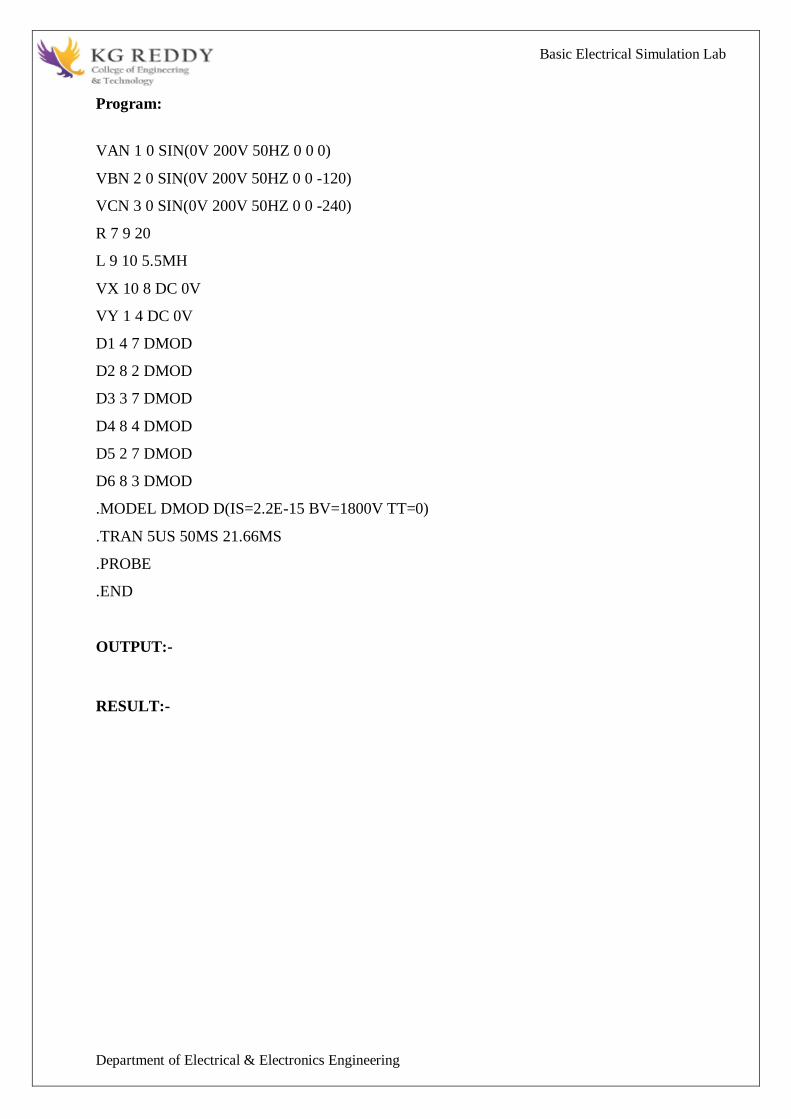
Basic Electrical Simulation Lab
Department of Electrical amp Electronics Engineering
PROGRAM
LOW PASS FILTER
N = 100 FIR filter order
Fp = 20e3 20 kHz passband-edge frequency
Fs = 96e3 96 kHz sampling frequency
Rp = 000057565 Corresponds to 001 dB peak-to-peak ripple
Rst = 1e-4 Corresponds to 80 dB stopband attenuation
eqnum = firceqrip(NFp(Fs2)[Rp Rst]passedge) eqnum = vec of coeffs
fvtool(eqnumFsFsColorWhite) Visualize filter
HIGH PASS FILTER
Fstop = 350
Fpass = 400
Astop = 65
Apass = 05
Fs = 1e3
d = designfilt(highpassfirStopbandFrequencyFstop
PassbandFrequencyFpassStopbandAttenuationAstop
PassbandRippleApassSampleRateFsDesignMethodequiripple)
fvtool(d)
OUTPUT-
RESULT-
Basic Electrical Simulation Lab
Department of Electrical amp Electronics Engineering
EXPERIMENT-13
FINDING THE EVEN AND ODD PARTS OF SIGNAL SEQUENCE AND REAL AND
IMAGINARY PARTS OF SIGNAL
AIM
program for finding even and odd parts of sequences Using OCTAVE Softwareamp
program for finding real and imaginary parts of sequences Using OCTAVE Software
APPARATUS
1 OCTAVE
2 LINUX
THEORY
Even and Odd Signal
One of characteristics of signal is symmetry that may be useful for signal analysis Even signals
are symmetric around vertical axis and Odd signals are symmetric about origin
Even Signal A signal is referred to as an even if it is identical to its time-reversed counterparts
x(t) = x(-t)
Odd Signal A signal is odd if x(t) = -x(-t)
An odd signal must be 0 at t=0 in other words odd signal passes the origin
Using the definition of even and odd signal any signal may be decomposed into a sum of its even
part xe(t) and its odd part xo(t) as follows
x(t)=xe(t)+xo(t)
x(t)=12x(t)+x(-t) +12x(t)-x(-t)
where
xe(t)=12x(t)+x(-t) ampxo(t)=12x(t)-x(-t)
It is an important fact because it is relative concept of Fourier series In Fourier series aperiodic
signal can be broken into a sum of sine and cosine signals Notice that sine function is odd signal
and cosine function is even signal
ENERGY AND POWER SIGNAL
A signal can be categorized into energy signal or power
signal An energy signal has a finite energy 0 lt E lt 1049279 In other words energy signals have
values only in the limited time duration For example a signal having only one square pulse is
energy signal A signal that decays exponentially has finite energy so it is also an energy signal
The power of an energy signal is 0 because of dividing finite energy by infinite time (or length)
If x(t) is a real-valued signal with Fourier transform X(f) and u(f) is the Heaviside step function
Basic Electrical Simulation Lab
Department of Electrical amp Electronics Engineering
then the function
contains only the non-negative frequency components of X(f) And the operation is reversible due
to the Hermitian property of X(f)
X(f) denotes the complex conjugate of X(f)
The inverse Fourier transform of Xa(f) is the analytic signal
where x^(t) is the Hilbert transform of x(t) and J is the imaginary unit
Basic Electrical Simulation Lab
Department of Electrical amp Electronics Engineering
PROGRAM-
Evenoddrealimaginary parts of a sequences
clc
clear all
close all
h=input(enter noof samples)
m=(h-1)2
n=-mm
x=input(enter sample values)
subplot(411)
stem(nxg)
xlabel(time)
ylabel(amplitude)
title(original sequence)
xmir=fliplr(x)
subplot(412)
stem(nxmirr)
xlabel(time)
ylabel(amplitude)
title(folded sequence)
even part of sequence
xeven=(x+xmir)2
subplot(413)
stem(nxevenr)
xlabel(time)
ylabel(amplitude)
title(even part of sequence)
odd part of sequence
xodd=(x-xmir)2
subplot(414)
stem(nxoddg)
xlabel(time)
ylabel(amplitude)
title(odd part of sequence)
Basic Electrical Simulation Lab
Department of Electrical amp Electronics Engineering
RealampImaginary parts of a sequences
clc
clear all
close all
y=input(enter complex numbers)
yreal=real(y)
disp(real values of y)
yreal
yimag=imag(y)
disp(imaginary values of y)
yimag
PROCEDURE-
1 Open OCTAVE
2 Open new script
3 Type the program
4 Save in current directory
5 Compile and Run the program
6 For the output see command window Figure window
OUTPUT-
RESULT-
Basic Electrical Simulation Lab
Department of Electrical amp Electronics Engineering
EXPERIMENT-14
FINDING THE FOURIER TRANSFORM OF A GIVEN SIGNAL AND PLOTTING ITS
MAGNITUDE AND PHASE SPECTRUM
AIM
Program for finding the fourier transform of a given signal Using OCTAVE Software amp Plotting
Its Magnitude And Phase Spectrum Using OCTAVE Software
APPARATUS
1 OCTAVE
2 LINUX
THEORY
The Fourier transform (FT) decomposes a function of time (a signal) into the
frequencies that make it up in a way similar to how a musical chord can be expressed as the
frequencies (or pitches) of its constituent notes The Fourier transform of a function of time itself
is a complex-valued function of frequency whose absolute value represents the amount of that
frequency present in the original function and whose complex argument is the phase offset of the
basic sinusoid in that frequency The Fourier transform is called the frequency domain
representation of the original signal The term Fourier transform refers to both the frequency
domain representation and the mathematical operation that associates the frequency domain
representation to a function of time The Fourier transform is not limited to functions of time but
in order to have a unified language the domain of the original function is commonly referred to as
the time domain For many functions of practical interest one can define an operation that
reverses this the inverse Fourier transformation also called Fourier synthesis of a frequency
domain representation combines the contributions of all the different frequencies to recover the
original function of time
Linear operations performed in one domain (time or frequency) have corresponding
operations in the other domain which are sometimes easier to perform The operation
of differentiation in the time domain corresponds to multiplication by the frequency[remark 1] so
some differential equations are easier to analyze in the frequency domain Also convolution in the
time domain corresponds to ordinary multiplication in the frequency domain Concretely this
means that any linear time-invariant system such as a filter applied to a signal can be expressed
relatively simply as an operation on frequencies After performing the desired operations
transformation of the result can be made back to the time domain Harmonic analysis is the
systematic study of the relationship between the frequency and time domains including the kinds
Basic Electrical Simulation Lab
Department of Electrical amp Electronics Engineering
of functions or operations that are simpler in one or the other and has deep connections to many
areas of modern mathematics
PROGRAM
Fs = 1000 Sampling frequency
T = 1Fs Sampling period
L = 1500 Length of signal
t = (0L-1)T Time vector
S = 07sin(2pi50t) + sin(2pi120t)
X = S + 2randn(size(t))
plot(1000t(150)X(150))
title(Signal Corrupted with Zero-Mean Random Noise)
xlabel(t (milliseconds))
ylabel(X(t))
Y = fft(X)
P2 = abs(YL)
P1 = P2(1L2+1)
P1(2end-1) = 2P1(2end-1)
f = Fs(0(L2))L
plot(fP1)
title(Single-Sided Amplitude Spectrum of X(t))
xlabel(f (Hz))
ylabel(|P1(f)|)
Y = fft(S)
P2 = abs(YL)
P1 = P2(1L2+1)
P1(2end-1) = 2P1(2end-1)
plot(fP1)
title(Single-Sided Amplitude Spectrum of S(t))
xlabel(f (Hz))
ylabel(|P1(f)|)
OUTPUT-
RESULT-

Basic Electrical Simulation Lab
Department of Electrical amp Electronics Engineering
of functions or operations that are simpler in one or the other and has deep connections to many
areas of modern mathematics
PROGRAM
Fs = 1000 Sampling frequency
T = 1Fs Sampling period
L = 1500 Length of signal
t = (0L-1)T Time vector
S = 07sin(2pi50t) + sin(2pi120t)
X = S + 2randn(size(t))
plot(1000t(150)X(150))
title(Signal Corrupted with Zero-Mean Random Noise)
xlabel(t (milliseconds))
ylabel(X(t))
Y = fft(X)
P2 = abs(YL)
P1 = P2(1L2+1)
P1(2end-1) = 2P1(2end-1)
f = Fs(0(L2))L
plot(fP1)
title(Single-Sided Amplitude Spectrum of X(t))
xlabel(f (Hz))
ylabel(|P1(f)|)
Y = fft(S)
P2 = abs(YL)
P1 = P2(1L2+1)
P1(2end-1) = 2P1(2end-1)
plot(fP1)
title(Single-Sided Amplitude Spectrum of S(t))
xlabel(f (Hz))
ylabel(|P1(f)|)
OUTPUT-
RESULT-


![[] Basic Electrical Circuits](https://static.fdocuments.us/doc/165x107/55cf8cc45503462b138f9bb8/-basic-electrical-circuits.jpg)