20 Years of VIX: Fear, Greed and Implications for Alternative Investment Strategies

20 years of VIX: Fear, Greed and Implications for Alternative Investment Strategies

The Abstract In this article, I investigate the statistical properties and relationships of VIX with alternative investment strategies. I find that different VIX states result in very different risk adjusted performance for all strategies and confirm that significant deviations from normality are observed in the states and the full sample, which are not fully captured by traditional risk metrics. I demonstrate that correlations among strategies are unstable and non-linear, leading to highly concentrated diversification benefits at the times of market stress, which a broad set of exposures is likely to negate. I also demonstrate that at certain states, correlations are very high between traditional and alternative investment strategies and performance characteristics are very similar. I establish that the superior, long term performance of such strategies relative to traditional asset classes is not due to higher returns in good times, but rather better preservation of capital in bad times. Based on empirical data, practical recommendations for investment analysis and risk management are included throughout the article. This is a companion article to ’20 years of VIX: Fear, Greed and Implications for Traditional Asset Classes’ (Munenzon (2010)) available at http://papers.ssrn.com/sol3/papers.cfm?abstract_id=1583504

Mikhail Munenzon, CFA, CAIA [email protected]

2

Introduction

Whaley (1993) introduced the VIX index. In the same year, the Chicago Board

Options Exchange (CBOE) introduced the CBOE Volatility Index and it quickly became

the benchmark for stock market volatility and, more broadly, investor sentiment. The

first VIX was a weighted measure of the implied volatility with 30 days to expiration

of eight S&P 100 at-the-money put and call options. Ten years later, it expanded to use

options based on a broader index, the SP 500, which allows for a more accurate view of

investors' expectations on future market volatility. On March 26, 2004, the first ever

trading in futures on the VIX index began on the CBOE. Based on the methodology for

SP 500, the index has historical information going back to the start of 1990.

Why should an investor care about volatility? Black (1975) suggested that the

informed investors would try to take advantage of their views through the options market

because of the leverage such instruments provided. Therefore, clues from the options

market may have implications for the performance characteristics of a security (for

example, see Bali and Hovakimian (2009) and Doran and Krieger (2010)). Moreover,

starting with the work of Engle (1982) and Bollerslev(1986), evidence emerged

documenting the clustering behavior of volatility1 and its resulting predictability.

Consequently, if different volatility states are associated with different performance

characteristics of a security, an investor’s investment and risk management policies will

need to be flexible enough to incorporate that such information.

1 High volatility is like to be followed by high volatility; low volatility is likely to be followed by low volatility.

3

Munenzon (2010) demonstrates that varying levels of VIX are associated with

very different return and risk characteristics of traditional asset classes. In this article, I

extend this analysis to 9 common alternative investment strategies as convertible

arbitrage (CA), distressed (DS), merger arbitrage (MA)(, commodity trading advisor

(CTA), macro, equity long/short (LS), equity market neutral (EMN), emerging markets

(EM), event driven (ED) (for more detail on strategies, the reader is referred to Anson

(2006)). I also evaluate relationships between traditional assets and alternative

investment strategies. This article is structured as follows. After an overview of data, I

will present key empirical results; concluding remarks follow.

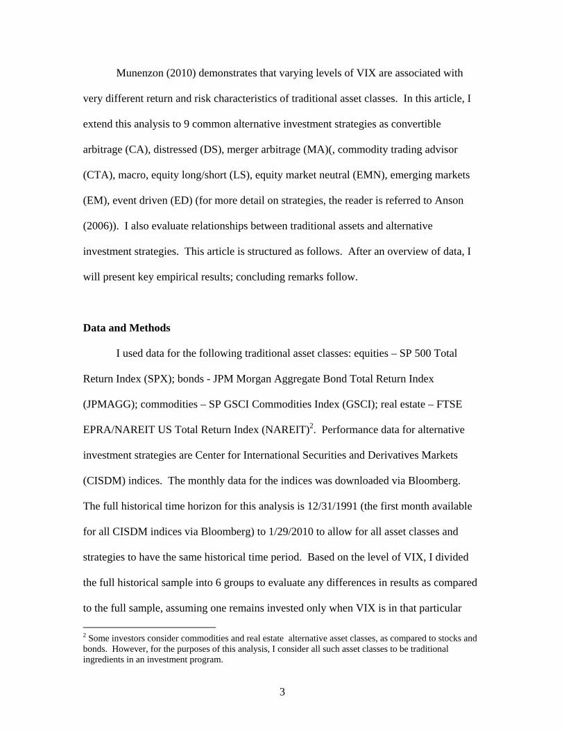
Data and Methods

I used data for the following traditional asset classes: equities – SP 500 Total

Return Index (SPX); bonds - JPM Morgan Aggregate Bond Total Return Index

(JPMAGG); commodities – SP GSCI Commodities Index (GSCI); real estate – FTSE

EPRA/NAREIT US Total Return Index (NAREIT)2. Performance data for alternative

investment strategies are Center for International Securities and Derivatives Markets

(CISDM) indices. The monthly data for the indices was downloaded via Bloomberg.

The full historical time horizon for this analysis is 12/31/1991 (the first month available

for all CISDM indices via Bloomberg) to 1/29/2010 to allow for all asset classes and

strategies to have the same historical time period. Based on the level of VIX, I divided

the full historical sample into 6 groups to evaluate any differences in results as compared

to the full sample, assuming one remains invested only when VIX is in that particular

2 Some investors consider commodities and real estate alternative asset classes, as compared to stocks and bonds. However, for the purposes of this analysis, I consider all such asset classes to be traditional ingredients in an investment program.

4

state. Such classification is broadly consistent with Figure 1 and practitioners’ views on

what constitutes low, medium and high volatility and provides a practical way of judging

any changes in performance and other characteristics of asset classes, given a VIX state.

Key Empirical Results

Figure 1 shows the historical level of VIX and cumulative return graphs for the

asset classes and VIX. Though the starting and ending points for VIX are relatively

comparable, the range of results is very high; one also finds that there are extended

periods of high and low volatility. The figure also suggests that crashes don’t just happen

– they are generally preceded by periods of increasing turbulence, which ultimately push

markets over the edge.

Table 1 presents key statistical information on VIX and alternative investment

strategies for the full historical period. For all the asset classes and strategies, cumulative

returns are strongly positive, especially real estate3. However, statistical features of

strategies have a broad range. As expected and similar to traditional asset classes,

strategies’ returns are strongly non-normal. The assumption that returns follow a normal

distribution, one of the fundamental assumptions of classical finance, can be strongly

rejected for all strategies4. However, not all strategies are equally non – normal and their

deviations from normality are not always the ones investors should try to avoid. For

example, some strategies such as convertible arbitrage, distressed, emerging markets and

event driven have very large kurtosis (fat tails or large extreme events as compared to the

normal distribution) and negative skewness (returns below the mean are more likely than

3 Secular decline in long term interest rates and the subsequent real estate bubble, which is still being resolved, also played key roles. 4 For a normal distribution, skewness should be 0 and kurtosis should be 3.

5

above the mean). These empirical features important for portfolio construction and risk

management are masked by the deceptively low volatility (see more below). Such

features (negative skewness and large kurtosis) are the opposite of what investors

typically prefer – positive skewness and small kurtosis, resulting in consistent, positive

returns. In contrast, CTA exhibits small positive skewness with relatively small kurtosis

while macro exhibits significant positive skewness with larger kurtosis, which is less

problematic in this case as extreme positive events are more likely than extreme negative

events. Figure 6 provides a graphical representation of the above results. One can

observe that most of the probability mass of returns for ED in its histogram is below the

typical observation with the left, negative tail being much larger than the right, positive

tail. By contrast, CTA’s probability mass is mostly above the typical observation with

the negative tail containing a smaller area than the right tail.

Not only does one not observe normality, but one also finds serial correlation for

most of the time series5, which is inconsistent with a random walk model. In classical

finance, correlation6, a linear measure of dependency, plays a key role in portfolio risk

measurement and optimization. In Table 4, one can see that in the full sample,

correlations within and across asset classes and strategies are relatively low (particularly,

between SPX vs GSCI, JPMAGG, CTA, Macro; GSCI vs Macro; EM vs CTA; CTA vs

NAREIT, CA and MA). Similar to traditional asset classes, all strategies with the

exception of CTA have significant negative correlation with VIX. It is also noteworthy

that relative to SPX, most strategies do not offer lower correlations than GSCI or

5 Positive returns are likely to be followed by positive returns and negative returns are likely to be followed by negative returns 6 Throughout the paper, correlation refers to what is more formally known as Pearson product-moment correlation coefficient, which is used extensively by practitioners and academics to model dependence.

6

JPAGG; some do not even improve on NAREIT correlation with SPX. Therefore,

depending on an investor’s goals and scenarios, an addition of a broad basket of

alternative strategies to a portfolio may not always provide meaningful incremental

benefit as compared to other traditional asset classes, which may be available much more

cheaply. A more selective addition of alternatives to one’s portfolio may result in greater

benefits because of the diversity of behavior of strategies among themselves and with

traditional asset classes. Finally, because of fat tails exacerbated by negative skewness,

historical VaR significantly understate realistic losses one can experience in adverse

scenarios, as measured by historical CVaR7. For instance, CA’s historical VAR at 95%

conference level is 1% but its CVaR(95%) is 3 times higher at 3.1%. Moreover, because

of high serial correlation resulting in ‘smooth’ returns, volatility masks the true extent of

tail losses8. For example, CA’s volatility in the full sample is only a little higher than that

of JPMAGG (1.2% vs 1.4%), but its worst loss is over 3 times higher (11.5% vs 3.5%).

Similarly, while CA’s volatility is slightly lower than that of Macro in the full sample

(1.4% vs 1.6%), its CVaRs and worst losses are much larger.

Which states dominated historically? The first state (VIX below 20%) accounted

for over 50% of all days in the historical sample due to extended periods of calm in the

90s and, to a lesser extent, in the middle of this decade (Table 6). The first 3 states (VIX

at up to 30%) accounted for over 90% of all days. However, as seen in the historical VIX

7 VaR(a) is defined as the probability of a loss less than or equal to quantity Q, with the confidence level of a. Thus, it stops at the start of extreme events and does not analyze the tail. CVaR(a) is defined as the average loss once Q is exceeded, with the confidence level of a. Historical based measures are evaluated based on historical data and thus fully incorporate all features of a distribution of a return series. If one assumes a normal distribution of returns, one can find VaR of a a return series via an analytical formula with just its mean and volatility. However, such a measure will understate the realistic extent of losses even more than the historical VaR. For more detail, the reader is referred to Alexander (2008). 8 Returns can be ‘unsmoothed’ to produce a more realistic picture of volatility and potential losses. For example, see Davies et al (2005).

7

chart, the last decade was far more volatile than the decade of the 90s. In addition, once

in states 1-3, VIX is likely to remain in that state for a period of time, as transitions occur

gradually. It is not possible to draw strong conclusions with available data for states 4-6

as the number of observations in each state is low. However, such a conclusion is

supported with daily data (see Munenzon (2010)). Moreover, even with available data,

one can observe that once in a high volatility state, one is likely to remain in one of the

high volatility states 4-6.

How similar are risk/return properties of strategies in various states and relative to

the full historical sample? Very dissimilar (Tables 2 and 3). In fact, evidence of

consistent, absolute returns in all market cycles is hard to find for alternative strategies.

Only CTA, macro and EMN (and bonds for traditional asset classes) provide

cumulatively positive returns across all the states. For all strategies, most of the

cumulative returns are made in states 1-3, particularly state 1; returns are mostly flat to

negative in higher states. This finding is very similar to that for traditional asset classes,

which are also very sensitive to VIX. However, not all strategies are sensitive to VIX in

the same way. While the percentage of positive months for strategies drops significantly

as VIX rises (Table 7), CTA responds well to a rising VIX and Macro and EMN manage

to maintain a high positive percentage even at high VIX levels. Finally, generally

superior, long term performance of alternative strategies relative to traditional asset

classes in the full sample came not from higher returns in good times but rather in

preserving a greater portion of those returns in bad times. For example, LS tracks SPX

relatively closely in good times but the downside is much more limited than SPX as

managers have full flexibility to adjust their portfolios to a particular environment. Also,

8

in state 1, SPX outperforms virtually all strategies but its losses are very large at stress

points of state 6, which significantly affects its cumulative return ranking in the full

sample.

How consistent are cumulative returns for asset classes in various states (Figures

2-4)? They are very consistent at the extreme states 1 and 6. In state 1, all are positive,

especially EM, ED, DS and LS. In state 6, CTA is consistently and meaningfully

positive; EMN and Macro are very slightly positive; all other strategies are negative.

Strategies exhibit a generally consistent behavior in other states as well. For example,

EM, ED and LS generally do not perform well as VIX rises; however, CTA, Macro and

EMN are generally positive across all states.

Given the prior discussion of returns in different states, it is not surprising to find

how unstable correlations are across states (Tables 4 and 5). For example, in state 1 (and

state 2 to a lesser extent), all indices (traditional assets and strategies) are highly

positively correlated. In state 6 (and state 5 to a lesser extent), most indices are also

highly positively correlated with the exception of CTA, Macro, EMN and JPMAGG. In

other states, the picture is more complex. However, correlations of strategies among

themselves and with traditional asset classes generally remain meaningful even if smaller

in magnitude than at extreme times. Evaluation of correlation for the full sample masks

such complex behavior. Additionally, such behavior suggests that not only are

dependencies among asset classes time varying, but that they are also non-linear.

Therefore, correlation may not be an appropriate means of evaluating dependence among

asset classes9. Moreover, while at the points of extreme stress, diversification can

9 Correlation will correctly describe dependence structure only in very particular cases, such as multivariate normal distributions. Also, at extremes, correlation should be zero for a multivariate normal distribution,

9

provide downside protection, such benefits are limited only to CTA, Macro and EMN

(and bonds for traditional asset classes). Finally, given the non-synchronized relationship

of VIX with traditional asset classes and alternative strategies, it should play a useful role

in an investment program by helping investors minimize potential losses and thus

enhance risk adjusted portfolio performance.

Conclusions

The level of VIX seems to have important and different implications for return

expectations for all alternative investment strategies. This is particularly true for the

extreme levels of VIX. Though the historical range for VIX is very broad, it exhibits

clustering, which make it useful for forecasting. I further present evidence that during the

historical period used in the article, several important assumptions of classical finance –

normal distribution, randomness of data (no serial correlation) and the use of correlation

to describe dependence – find limited support in empirical data. In the cases of large

deviations from normality and in the presence of serial correlation, which are typically

larger among alternative investment strategies as compared to traditional asset classes,

volatility and VaR metrics fail to capture the risk of losses appropriately. A focus on

volatility with alternative strategies may overlook large, potential losses hidden in the

tails, which volatility cannot capture. Therefore, a practitioner should generate value by

incorporating more realistic assumptions to model markets for investment analysis and

risk management, such as non-normal distributions which can incorporate skews and fat

tails of returns, adjustments for ‘smooth’ data and copulas which can capture non-

linearity of dependencies, particularly in the tails.

which is not empirically supported. For a more detailed critique on the use of correlations to model dependence, see Embrechts et al (2002).

10

The diversity of behavior of alternative investment strategies among themselves

and with traditional asset classes suggests that such strategies may add significant value

in portfolio construction and risk management but each strategy’s role and value may

vary significantly depending on an investor’s goals, risk tolerance and investment

environment scenarios. Generally superior, long term performance of alternative

strategies relative to traditional asset classes is not due to better returns in good times but

rather relatively more contained losses. While the return potential of alternative

strategies may have eroded due to the significant rise in asset since the early 90s (see

Figure 5, particularly CA, Macro, EMN and MA), downside management capabilities

should remain intact if managers have flexible investment mandates and risk

management discipline. The cost of very low volatility with respectable returns is

significant negative skewness and kurtosis resulting in much larger extreme losses than

volatility may suggest (e.g., CA, ED). However, some strategies possess positive

skewness and well contained tails (e.g., CTA and Macro). Evidence for consistent,

absolute returns is limited. Masked within the full sample is the fact that risk/return

characteristics of strategies across states are very different – e.g., CTA strongly

outperforms in state 6 but EM outperforms in state 1. Most strategies performance

deteriorates rapidly as VIX rises; CTA is the only strategy that responds well to a rising

level of VIX. Moreover, alternative strategies are much more highly correlated with each

other and traditional asset classes than the full sample may suggest, with almost perfect

correlation at extremes. At stress points, only CTA, Macro and EMN help preserve and

add to capital (particularly, CTA). Thus, as with traditional asset classes, diversification

is possible but its benefits are highly concentrated, which a broad set of exposures dilutes.

11

Interestingly, strategies and assets optimal for stressed periods (e.g., bonds, CTA, EMN)

are those an investor may want to minimize in a portfolio to optimize returns in a good

environment. Also, given the performance characteristics of VIX and its relationship

with other assets and strategies, its inclusion in an investment program should provide

valuable benefits in risk management.

The analytical framework presented in this article can be refined further by adding

more factors deemed important, such as inflation or information about the prior VIX

state; it can also be extended to sectors within an asset class and alternative investment

strategies. Finally, while we do not know which volatility states will dominate in the

future or how long they may last, greater awareness of the current investment

environment, its implications for risk adjusted performance and flexible investment

policies to position portfolios appropriately should help investors produce more

consistent results.

References

Anson, M. 2006. Handbook of Alternative Assets. John Wiley and Sons.

Alexander, C. 2008. Value at Risk Models. John Wiley & Sons.

Bali, T. and A. Hovakimian. 2009. “Volatility Spreads and Expected stock Returns.”

Management Science, vol. 55, no. 11 (November): 1797-1812.

Black, F. 1975. “Fact and Fantasy in the Use of Options.” Financial Analysts Journal,

vol. 31, no. 4 (July/August): 36-41.

Bollerslev, T. 1986. “Generalized Autoregressive Conditional Heteroskedasticity.”

Journal of Econometrics 31: 307-327.

12

Davies, R., Kat, H. and Lu, S. 2005. “Fund of Hedge Funds Portfolio Selection: A

Multiple Objective Approach.” Working Paper.

Doran J. and K. Krieger. 2010. “Implications for Asset Returns in the Implied Volatility

Skew.” Financial Analysts Journal, vol. 66, no, 1 (January/February): 65-76.

Engle, R. 1982. “Autoregressive Conditional Heteroskedasticity with Estimates of the

Variance of UK inflation.” Econometrica 50: 987-1007.

Embrechts, P, A. McNeil, and D. Straumann. 2002. “Correlation and dependence in risk

management: Properties and Pitfalls.” In M. Dempster (e.d), Risk Management: Value at

Risk and Beyond. Cambridge University Press.

Munenzon, M. 2010. “20 Years of VIX: Fear, Greed and Implications for Traditional

Asset Classes.” Working Paper.

Whaley, R. 1993. “Derivatives on Market Volatility: Hedging Tools Long Overdue.”

Journal of Derivatives, 1 (Fall): 71-84.

Figure 1

Historical VIX (12/31/1991 - 1/29/2010)

0

10

20

30

40

50

60

70

12

/31

/19

91

12

/15

/19

92

11

/30

/19

93

11

/15

/19

94

10

/31

/19

95

10

/15

/19

96

9/3

0/1

99

7

9/1

5/1

99

8

8/3

1/1

99

9

8/1

5/2

00

0

7/3

1/2

00

1

7/1

6/2

00

2

7/1

/20

03

6/1

5/2

00

4

5/3

1/2

00

5

5/1

6/2

00

6

5/1

/20

07

4/1

5/2

00

8

3/3

1/2

00

9

Date

VIX

Cumulative Return - Full Historical Sample

0

1

2

3

4

5

6

7

8

9

12

/31

/19

91

10

/26

/19

92

8/2

2/1

99

3

6/1

8/1

99

4

4/1

4/1

99

5

2/8

/19

96

12

/4/1

99

6

9/3

0/1

99

7

7/2

7/1

99

8

5/2

3/1

99

9

3/1

8/2

00

0

1/1

2/2

00

1

11

/8/2

00

1

9/4

/20

02

7/1

/20

03

4/2

6/2

00

4

2/2

0/2

00

5

12

/17

/20

05

10

/13

/20

06

8/9

/20

07

6/4

/20

08

3/3

1/2

00

9

1/2

5/2

01

0

Date

Cu

mu

lati

ve

Re

turn

CA DS MA CTA Macro LS EMN EM ED

Figure 2

Cumulative Return - State 1 of VIX (<=20)

0

1

2

3

4

5

6

'12

/31

/19

91

'

'4/3

0/1

99

2'

'9/3

0/1

99

2'

'2/2

6/1

99

3'

'7/3

0/1

99

3'

'12

/31

/19

93

'

'6/3

0/1

99

4'

'11

/30

/19

94

'

'4/2

8/1

99

5'

'9/2

9/1

99

5'

'2/2

9/1

99

6'

'7/3

1/1

99

6'

'1/3

0/1

99

8'

'2/2

8/2

00

2'

'7/3

1/2

00

3'

'1/3

0/2

00

4'

'6/3

0/2

00

4'

'11

/30

/20

04

'

'4/2

9/2

00

5'

'9/3

0/2

00

5'

'2/2

8/2

00

6'

'7/3

1/2

00

6'

'12

/29

/20

06

'

'5/3

1/2

00

7'

Date

Cu

mu

lati

ve

Re

turn


Cumulative Return - State 2 of VIX (>20 and <=25)

0.91

1.11.21.31.41.51.61.71.81.9

'2/2

8/1

99

4'

'12

/31

/19

96

'

'3/3

1/1

99

7'

'7/3

1/1

99

7'

'12

/31

/19

97

'

'4/3

0/1

99

8'

'2/2

6/1

99

9'

'7/3

0/1

99

9'

'11

/30

/19

99

'

'2/2

9/2

00

0'

'8/3

1/2

00

0'

'4/3

0/2

00

1'

'10

/31

/20

01

'

'1/3

1/2

00

2'

'8/2

9/2

00

3'

'10

/31

/20

07

'

'5/3

0/2

00

8'

'10

/30

/20

09

'

Date

Cu

mu

lati

ve

Re

turn


Figure 3

Cumulatiave Return - State of VIX (>25 and <=30)

0.9

1

1.1

1.2

1.3

1.4

1.5

'10

/31

/19

97

'

'9/3

0/1

99

8'

'12

/31

/19

98

'

'3/3

1/1

99

9'

'8/3

1/1

99

9'

'10

/31

/20

00

'

'1/3

1/2

00

1'

'3/3

0/2

00

1'

'10

/31

/20

02

'

'1/3

1/2

00

3'

'12

/31

/20

07

'

'2/2

9/2

00

8'

'5/2

9/2

00

9'

'7/3

1/2

00

9'

Date

Cu

mu

lati

ve

Re

turn



0.9

0.95

1

1.05

1.1

1.15

'8/3

1/2

00

1'

'8/3

1/2

00

1'

'9/2

8/2

00

1'

'6/2

8/2

00

2'

'7/3

1/2

00

2'

'9/3

0/2

00

2'

'12

/31

/20

02

'

'9/3

0/2

00

9'

Date

Cu

mu

lati

ve

Re

turn


Figure 4


0.8

0.85

0.9

0.95

1

1.05

'9/3

0/1

99

7'

'9/3

0/1

99

7'

'8/3

0/2

00

2'

'8/2

9/2

00

8'

'11

/28

/20

08

'

'3/3

1/2

00

9'

Date

Cu

mu

lati

ve

Re

turn


Cumulative Return - State 6 of VIX (>40)

0.5

0.6

0.7

0.8

0.9

1

1.1

1.2

'7/3

1/1

99

8'

'7/3

1/1

99

8'

'8/3

1/1

99

8'

'9/3

0/2

00

8'

'10

/31

/20

08

'

'12

/31

/20

08

'

'1/3

0/2

00

9'

'2/2

7/2

00

9'

Date

Cu

mu

lati

ve

Re

turn


Figure 5

Cumulative Returns with 4 Year Rolling Window - Selected Alternatives as of 1/29/10

-0.4

-0.2

0

0.2

0.4

0.6

0.8

1

1.2

12/29/1995 9/24/1998 6/20/2001 3/16/2004 12/11/2006 9/6/2009

Date

Cu

mu

lati

ve

Re

turn

CA DS MA CTA EMN Macro EM

Figure 6

-0.08 -0.06 -0.04 -0.02 0 0.02 0.04 0.060

10

20

30

40

50

60

70

80

Histogram of CISDM Event Driven Index Monthly Returns12/31/1991 - 1/29/2010

-0.06 -0.04 -0.02 0 0.02 0.04 0.06 0.080

10

20

30

40

50

60

Histogram of CISDM CTA Index Monthly Returns12/31/1991 - 1/29/2010

Table 112/31/1991 - 1/31/2010 SPX GSCI NAREIT JPMAGG VIX CA DS MA CTA Macro LS EMN EM EDmonthly dataArithmetic avg return 0.7% 0.7% 1.1% 0.5% 1.5% 0.8% 0.9% 0.8% 0.7% 0.8% 1.0% 0.7% 0.9% 1.0%Compounded avg return 0.6% 0.5% 0.9% 0.5% 0.1% 0.8% 0.9% 0.8% 0.7% 0.8% 0.9% 0.7% 0.8% 0.9%max 9.8% 21.1% 31.7% 4.6% 90.8% 4.7% 5.3% 4.7% 7.9% 8.6% 9.4% 2.8% 12.1% 4.8%min -16.8% -27.8% -32.2% -3.5% -32.7% -11.5% -10.6% -5.6% -5.4% -5.4% -9.4% -2.1% -26.3% -7.3%vol 4.3% 6.1% 6.0% 1.2% 17.9% 1.4% 1.8% 1.1% 2.5% 1.6% 2.2% 0.6% 3.8% 1.7%Normality at 95% confidence level? No No No No No No No No No No No No No Nopval 0.1% 0.1% 0.1% 2.3% 0.1% 0.1% 0.1% 0.1% 4.5% 0.1% 0.1% 0.1% 0.1% 0.1%No serial correlation at 95% confidence level? Yes No No Yes No No No No Yes No Yes No No Nopval 69% 0% 0% 51% 35% 0% 0% 0% 20% 4% 7% 0% 0% 0%VaR (95%) -7.6% -9.4% -7.8% -1.4% -21.1% -1.0% -1.5% -1.0% -3.3% -1.2% -2.4% -0.1% -4.4% -1.5%VaR (99%) -12.1% -14.3% -22.3% -2.7% -29.9% -4.4% -6.0% -2.4% -4.4% -2.5% -4.5% -1.1% -12.6% -6.9%CVaR(95%) -10.1% -12.9% -15.0% -2.1% -26.4% -3.1% -3.9% -2.0% -4.0% -2.2% -3.9% -0.7% -9.2% -3.7%CVaR(99%) -14.0% -19.2% -25.9% -2.9% -31.1% -7.4% -8.1% -3.5% -4.8% -3.6% -6.3% -1.5% -17.6% -7.1%Skewness -0.8 -0.3 -0.9 -0.2 1.4 -3.9 -1.9 -0.8 0.4 1.2 -0.2 -0.4 -2.1 -1.6Kurtosis 4.4 5.2 11.6 3.9 6.8 33.6 13.4 8.7 3.0 7.6 5.7 6.3 16.0 9.4cumulative return for full sample 269.32% 174.79% 604.87% 214.90% 27.50% 435.40% 596.83% 450.51% 306.00% 413.66% 637.00% 322.57% 516.20% 651.63%% of months with positive returns 64.1% 56.2% 65.0% 68.2% 46.5% 85.7% 79.7% 86.2% 55.3% 71.0% 70.0% 92.2% 71.4% 80.2%

Notes:Jarque-Bera test was used to evaluate normality of a time series; null hypothesis is stated in the question.Ljung-Box test with 20 lags was used to evaluate serial correlation of a time series;null hypothesis is stated in the question.SPX - SP500 Total ReturnGSCI - SP GSCI NAREIT - FTSE EPRA/NAREIT US Total ReturnJPMAGG - JPM Morgan Aggregate Bond Total ReturnVIX - VIX IndexCA - convertible arbitrageDS - distressedLS - equity long/shortMA - merger arbitrageEM - emerging marketsEMN - equity market neutralED - event driven

Table 2State 1 - VIX <= 20 SPX GSCI NAREIT JPMAGG VIX CA DS MA CTA Macro LS EMN EM EDmonthly dataArithmetic avg return 1.5% 1.4% 1.9% 0.5% -1.0% 0.8% 1.3% 1.0% 0.7% 1.0% 1.4% 0.7% 1.5% 1.3%Compounded avg return 1.4% 1.3% 1.8% 0.4% -2.1% 0.8% 1.3% 1.0% 0.6% 1.0% 1.4% 0.7% 1.5% 1.3%max 7.6% 15.7% 8.6% 3.7% 48.0% 3.0% 5.3% 4.7% 6.2% 8.6% 6.3% 2.2% 8.5% 4.4%min -4.4% -9.9% -14.0% -3.5% -32.7% -2.5% -4.2% -1.0% -5.4% -5.4% -3.4% -1.3% -5.8% -1.6%vol 2.4% 5.0% 3.7% 1.1% 14.7% 0.8% 1.5% 1.0% 2.3% 1.8% 1.6% 0.5% 2.4% 1.2%Normality at 95% confidence level? Yes Yes No No No No No No Yes No Yes No Yes Yespval 50.0% 15.4% 0.1% 2.5% 0.2% 0.1% 0.9% 0.1% 30.5% 0.1% 38.0% 0.1% 5.7% 50.0%No serial correlation at 95% confidence level? Yes Yes No Yes No No No No No Yes Yes Yes No Yespval 45.5% 5.8% 2.5% 23.6% 3.6% 0.0% 10.3% 1.8% 1.8% 13.3% 59.3% 15.0% 0.4% 25.4%VaR (95%) -2.5% -6.8% -4.0% -1.4% -20.0% -0.7% -1.2% -0.7% -2.7% -1.2% -1.3% 0.1% -2.3% -0.8%VaR (99%) -3.9% -9.5% -10.8% -2.9% -30.3% -1.6% -3.0% -1.0% -4.6% -2.9% -2.7% -0.5% -5.8% -1.5%CVaR(95%) -3.2% -8.4% -7.7% -2.2% -25.4% -1.3% -2.1% -0.9% -3.6% -2.1% -2.1% -0.3% -3.9% -1.2%CVaR(99%) -4.0% -9.7% -11.7% -3.1% -30.9% -1.9% -3.3% -1.0% -4.8% -3.6% -2.9% -0.7% -5.8% -1.5%Skewness -0.1 0.3 -1.0 -0.5 0.9 -1.0 -0.3 0.8 0.3 1.1 -0.1 -0.4 -0.1 0.0Kurtosis 2.8 3.4 5.1 3.8 4.3 5.1 4.5 5.3 2.8 7.2 3.5 5.7 4.0 3.1cumulative return 435.1% 342.0% 697.7% 68.9% -91.3% 154.3% 340.7% 229.1% 112.9% 211.6% 398.2% 134.8% 463.0% 340.4%% of months with positive returns 77.1% 62.7% 73.7% 64.4% 40.7% 86.4% 85.6% 91.5% 55.1% 73.7% 79.7% 96.6% 79.7% 86.4%

State 2 - VIX > 20 & <= 25 SPX GSCI NAREIT JPMAGG VIX CA DS MA CTA Macro LS EMN EM EDmonthly dataArithmetic avg return 0.7% -0.1% 0.7% 0.5% 2.5% 0.8% 0.9% 0.8% 0.1% 0.6% 1.0% 0.7% 1.1% 1.0%Compounded avg return 0.6% -0.3% 0.6% 0.5% 1.2% 0.8% 0.9% 0.8% 0.0% 0.6% 1.0% 0.7% 1.0% 1.0%max 9.8% 17.7% 10.8% 2.9% 44.9% 2.7% 3.9% 2.8% 6.1% 5.7% 9.4% 2.8% 12.1% 4.4%min -8.4% -11.9% -10.9% -2.0% -29.0% -1.6% -1.5% -1.9% -4.5% -3.0% -2.4% -0.7% -11.3% -1.6%vol 4.4% 5.8% 4.7% 1.1% 16.9% 0.9% 1.3% 1.0% 2.3% 1.4% 2.5% 0.7% 3.7% 1.4%Normality at 95% confidence level? Yes Yes Yes Yes Yes No Yes Yes Yes No No Yes No Yespval 28.0% 29.4% 50.0% 50.0% 20.7% 2.7% 43.8% 50.0% 50.0% 0.3% 0.5% 6.5% 1.4% 50.0%No serial correlation at 95% confidence level? No Yes Yes Yes Yes Yes Yes Yes Yes Yes Yes No No Yespval 0.1% 76.8% 20.4% 89.2% 35.2% 6.0% 21.2% 15.5% 80.4% 81.0% 40.8% 0.5% 0.1% 45.7%VaR (95%) -6.0% -8.1% -7.9% -1.4% -19.9% -1.2% -1.3% -1.2% -3.8% -1.2% -2.2% -0.3% -4.3% -1.2%VaR (99%) -8.4% -11.8% -10.9% -2.0% -28.9% -1.6% -1.5% -1.9% -4.5% -3.0% -2.4% -0.7% -11.2% -1.6%CVaR(95%) -6.9% -9.8% -9.4% -1.7% -25.5% -1.5% -1.4% -1.6% -4.2% -2.1% -2.3% -0.5% -7.0% -1.4%CVaR(99%) -8.4% -11.9% -10.9% -2.0% -29.0% -1.6% -1.5% -1.9% -4.5% -3.0% -2.4% -0.7% -11.3% -1.6%Skewness 0.1 0.4 -0.2 -0.1 0.4 -0.8 0.2 -0.2 0.1 0.8 1.2 0.5 -0.4 0.2Kurtosis 2.1 3.3 2.8 2.9 2.6 3.9 2.4 3.5 3.0 5.6 4.5 3.9 5.1 2.5cumulative return 40.0% -13.1% 34.9% 32.4% 89.1% 49.3% 59.0% 52.0% 2.3% 34.1% 69.4% 47.0% 68.9% 70.4%% of months with positive returns 50.9% 45.3% 56.6% 71.7% 49.1% 84.9% 79.2% 86.8% 50.9% 66.0% 64.2% 90.6% 67.9% 79.2%

State 3 - VIX > 25 & <= 30 SPX GSCI NAREIT JPMAGG VIX CA DS MA CTA Macro LS EMN EM EDmonthly dataArithmetic avg return 0.2% 0.9% 2.5% 0.5% 0.2% 1.3% 0.9% 0.6% 1.4% 0.7% 0.4% 0.6% 0.7% 0.9%Compounded avg return 0.0% 0.6% 2.4% 0.5% -0.8% 1.3% 0.9% 0.6% 1.3% 0.6% 0.4% 0.6% 0.7% 0.8%max 8.1% 21.1% 14.2% 2.1% 28.8% 4.7% 4.9% 2.6% 7.9% 5.6% 4.8% 2.1% 9.5% 4.8%min -9.1% -16.6% -4.7% -2.7% -31.5% -2.4% -2.6% -1.6% -4.3% -2.1% -4.1% -1.0% -6.4% -3.2%vol 5.3% 7.5% 4.7% 1.0% 14.1% 1.4% 1.6% 0.9% 3.3% 1.5% 2.4% 0.7% 3.8% 1.7%Normality at 95% confidence level? Yes Yes Yes No Yes No Yes Yes Yes No Yes Yes Yes Yespval 20.9% 27.1% 11.7% 1.9% 50.0% 5.0% 50.0% 50.0% 38.0% 0.3% 50.0% 50.0% 50.0% 27.2%No serial correlation at 95% confidence level? Yes Yes Yes Yes Yes Yes Yes No Yes Yes Yes Yes Yes Yespval 33.1% 91.7% 59.0% 68.4% 83.7% 89.1% 84.7% 0.2% 49.0% 80.6% 53.6% 46.7% 95.7% 61.5%VaR (95%) -8.1% -11.1% -3.8% -1.3% -23.3% -0.3% -1.5% -1.3% -3.8% -1.2% -3.3% -0.8% -5.2% -3.1%VaR (99%) -9.1% -16.6% -4.7% -2.7% -31.5% -2.4% -2.6% -1.6% -4.3% -2.1% -4.1% -1.0% -6.4% -3.2%CVaR(95%) -8.5% -13.4% -4.1% -1.9% -26.7% -1.1% -2.0% -1.4% -4.0% -1.6% -3.7% -0.9% -5.7% -3.1%CVaR(99%) -9.1% -16.6% -4.7% -2.7% -31.5% -2.4% -2.6% -1.6% -4.3% -2.1% -4.1% -1.0% -6.4% -3.2%Skewness -0.1 0.3 0.7 -0.9 0.1 0.2 0.3 -0.2 0.4 1.3 0.0 -0.3 0.4 -0.5Kurtosis 1.8 4.0 2.9 4.8 3.2 4.9 3.3 3.6 2.4 6.1 2.2 3.4 3.0 3.7cumulative return 0.4% 16.9% 88.5% 14.7% -19.8% 43.0% 26.3% 17.1% 43.4% 18.9% 10.1% 16.7% 19.6% 25.3%% of months with positive returns 51.9% 51.9% 70.4% 74.1% 51.9% 96.3% 74.1% 81.5% 59.3% 74.1% 59.3% 81.5% 63.0% 77.8%


Table 3State 4 - VIX > 30 & <= 35 SPX GSCI NAREIT JPMAGG VIX CA DS MA CTA Macro LS EMN EM EDmonthly dataArithmetic avg return -1.3% 0.4% -4.3% 1.0% 9.8% 0.8% 0.4% -0.2% 1.1% 0.1% -0.8% 0.2% 0.2% -0.2%Compounded avg return -1.4% 0.2% -4.3% 1.0% 8.5% 0.8% 0.4% -0.2% 1.0% 0.1% -0.8% 0.2% 0.2% -0.2%max 8.8% 7.8% 0.2% 2.1% 28.1% 2.1% 1.6% 0.8% 3.2% 1.5% 1.1% 0.8% 2.5% 1.3%min -8.1% -10.5% -7.3% -0.3% -21.5% -0.7% -1.3% -2.0% -3.3% -1.8% -3.4% -0.3% -4.0% -2.9%vol 5.9% 6.9% 2.4% 0.9% 17.2% 0.8% 1.2% 1.0% 2.7% 1.1% 1.7% 0.4% 2.3% 1.7%Normality at 95% confidence level? Yes Yes Yes Yes Yes Yes Yes Yes Yes Yes Yes Yes Yes Yespval 50.0% 50.0% 44.4% 44.6% 48.1% 50.0% 28.4% 20.8% 12.3% 50.0% 21.7% 50.0% 14.6% 11.0%No serial correlation at 95% confidence level? Yes Yes Yes Yes Yes Yes Yes Yes Yes Yes Yes No Yes Yespval 80.1% 98.5% 6.9% 26.3% 80.5% 30.4% 48.2% 12.5% 68.3% 24.2% 16.5% 0.8% 33.0% 31.8%VaR (95%) -8.1% -10.5% -7.3% -0.3% -21.5% -0.7% -1.3% -2.0% -3.3% -1.8% -3.4% -0.3% -4.0% -2.9%VaR (99%) -8.1% -10.5% -7.3% -0.3% -21.5% -0.7% -1.3% -2.0% -3.3% -1.8% -3.4% -0.3% -4.0% -2.9%CVaR(95%) -8.1% -10.5% -7.3% -0.3% -21.5% -0.7% -1.3% -2.0% -3.3% -1.8% -3.4% -0.3% -4.0% -2.9%CVaR(99%) -8.1% -10.5% -7.3% -0.3% -21.5% -0.7% -1.3% -2.0% -3.3% -1.8% -3.4% -0.3% -4.0% -2.9%Skewness 0.4 -0.3 0.7 -0.2 -0.7 -0.4 -0.5 -0.8 -0.8 -0.6 -0.7 0.1 -0.9 -0.8Kurtosis 2.4 1.8 2.9 1.6 2.6 3.3 1.7 2.3 2.0 2.8 1.9 1.9 2.4 1.9cumulative return -9.6% 1.4% -26.4% 6.9% 77.2% 5.6% 2.9% -1.6% 7.4% 0.8% -5.6% 1.6% 1.1% -1.4%% of months with positive returns 42.9% 57.1% 14.3% 85.7% 85.7% 85.7% 71.4% 57.1% 71.4% 57.1% 42.9% 85.7% 71.4% 71.4%

State 5 - VIX > 35 & <= 40 SPX GSCI NAREIT JPMAGG VIX CA DS MA CTA Macro LS EMN EM EDmonthly dataArithmetic avg return -2.5% -2.4% 8.3% 1.1% 24.1% 0.4% -0.3% 0.3% 0.5% 0.4% -0.9% 0.1% -1.6% -1.1%Compounded avg return -2.8% -2.7% 7.5% 1.1% 16.3% 0.3% -0.3% 0.2% 0.5% 0.4% -0.9% 0.1% -1.8% -1.2%max 9.6% 5.7% 31.7% 3.4% 90.8% 4.6% 3.0% 2.1% 2.5% 1.2% 3.2% 1.2% 8.6% 2.0%min -10.9% -12.1% -4.3% -1.1% -27.6% -8.4% -4.4% -2.6% -1.2% -0.2% -5.4% -2.1% -10.1% -7.3%vol 8.2% 8.4% 15.6% 1.7% 49.2% 5.1% 2.7% 1.8% 1.7% 0.7% 3.2% 1.3% 6.9% 3.6%Normality at 95% confidence level? Yes Yes Yes Yes Yes Yes Yes Yes Yes Yes Yes Yes Yes Yespval 50.0% 18.9% 24.6% 50.0% 50.0% 5.7% 50.0% 27.6% 44.2% 17.3% 50.0% 7.7% 50.0% 6.4%No serial correlation at 95% confidence level? Yes Yes Yes Yes Yes Yes Yes Yes Yes No Yes Yes Yes Yespval 16.9% 25.5% 19.8% 19.4% 88.5% 54.8% 52.4% 59.3% 4.7% 0.9% 64.8% 22.5% 76.7% 24.8%VaR (95%) -10.9% -12.1% -4.3% -1.1% -27.6% -8.4% -4.4% -2.6% -1.2% -0.2% -5.4% -2.1% -10.0% -7.3%VaR (99%) -10.9% -12.1% -4.3% -1.1% -27.6% -8.4% -4.4% -2.6% -1.2% -0.2% -5.4% -2.1% -10.1% -7.3%CVaR(95%) -10.9% -12.1% -4.3% -1.1% -27.6% -8.4% -4.4% -2.6% -1.2% -0.2% -5.4% -2.1% -10.1% -7.3%CVaR(99%) -10.9% -12.1% -4.3% -1.1% -27.6% -8.4% -4.4% -2.6% -1.2% -0.2% -5.4% -2.1% -10.0% -7.3%Skewness 0.5 -0.3 0.7 0.0 0.3 -1.2 -0.5 -0.9 0.2 0.4 -0.2 -1.1 0.4 -1.2Kurtosis 1.9 1.2 1.8 1.9 1.6 2.9 2.5 2.5 1.4 1.3 2.1 2.7 2.2 2.9cumulative return -13.1% -12.6% 43.4% 5.8% 112.6% 1.3% -1.7% 1.2% 2.4% 2.0% -4.4% 0.4% -8.8% -5.8%% of months with positive returns 40.0% 60.0% 40.0% 80.0% 60.0% 80.0% 60.0% 80.0% 60.0% 60.0% 40.0% 80.0% 40.0% 40.0%

State 6 - VIX > 40 SPX GSCI NAREIT JPMAGG VIX CA DS MA CTA Macro LS EMN EM EDmonthly dataArithmetic avg return -6.1% -4.3% -13.7% 1.2% 18.0% -1.1% -3.4% -0.8% 2.5% 0.1% -1.8% 0.4% -6.8% -2.1%Compounded avg return -6.5% -5.2% -14.7% 1.2% 14.4% -1.2% -3.5% -0.8% 2.4% 0.1% -1.8% 0.4% -7.3% -2.1%max 8.8% 12.3% 6.3% 4.6% 78.6% 3.9% 1.1% 1.3% 7.2% 1.1% 1.7% 0.9% 3.5% 1.8%min -16.8% -27.8% -32.2% -2.0% -7.7% -11.5% -10.6% -5.6% -2.0% -2.3% -9.4% 0.0% -26.3% -7.3%vol 9.9% 13.2% 14.3% 2.4% 33.9% 5.0% 4.6% 2.4% 3.4% 1.1% 3.9% 0.3% 10.3% 3.7%Normality at 95% confidence level? Yes Yes Yes Yes Yes No Yes No Yes No Yes Yes Yes Yespval 27.3% 50.0% 50.0% 50.0% 10.1% 1.8% 14.7% 4.6% 47.3% 1.2% 5.5% 50.0% 8.9% 32.0%No serial correlation at 95% confidence level? Yes Yes Yes Yes Yes Yes Yes Yes Yes Yes Yes Yes Yes Yespval 46.0% 78.0% 87.0% 27.1% 20.2% 86.1% 82.3% 70.6% 27.0% 89.5% 52.6% 84.1% 69.8% 91.2%VaR (95%) -16.8% -27.8% -32.2% -2.0% -7.7% -11.5% -10.6% -5.6% -2.0% -2.3% -9.4% 0.0% -26.3% -7.3%VaR (99%) -16.8% -27.8% -32.2% -2.0% -7.7% -11.5% -10.6% -5.6% -2.0% -2.3% -9.4% 0.0% -26.3% -7.3%CVaR(95%) -16.8% -27.8% -32.2% -2.0% -7.7% -11.5% -10.6% -5.6% -2.0% -2.3% -9.4% 0.0% -26.3% -7.3%CVaR(99%) -16.8% -27.8% -32.2% -2.0% -7.7% -11.5% -10.6% -5.6% -2.0% -2.3% -9.4% 0.0% -26.3% -7.3%Skewness 0.6 -0.6 0.3 0.0 1.0 -1.5 -0.8 -1.3 0.1 -1.6 -1.2 0.1 -1.1 -0.5Kurtosis 1.8 2.6 1.7 1.7 2.3 4.1 1.9 3.3 1.6 4.1 3.3 1.7 2.8 1.7cumulative return -37.4% -31.0% -67.1% 8.6% 155.7% -7.9% -22.2% -5.7% 18.2% 0.7% -12.1% 2.9% -41.2% -13.9%% of months with positive returns 28.6% 42.9% 28.6% 57.1% 57.1% 42.9% 28.6% 42.9% 57.1% 71.4% 42.9% 85.7% 14.3% 28.6%


Table 4Correlation Matrices

Full SampleSPX GSCI NAREIT JPMAGG VIX CA DS MA CTA Macro LS EMN EM ED

SPX 1GSCI 0.166019 1NAREIT 0.53491 0.138621 1JPMAGG 0.050299 0.025469 0.086042 1VIX -0.62321 -0.15603 -0.34092 -0.04614 1CA 0.419011 0.291283 0.394769 0.163013 -0.38292 1DS 0.577209 0.275929 0.46886 0.021617 -0.44175 0.669364 1MA 0.524669 0.115169 0.355637 0.032789 -0.48047 0.510831 0.673551 1CTA -0.11897 0.177433 -0.05343 0.252222 0.057434 -0.07251 -0.15321 -0.10711 1Macro 0.344947 0.092964 0.149527 0.181607 -0.25827 0.232467 0.441577 0.469438 0.259513 1LS 0.724026 0.249474 0.351369 -0.02816 -0.50077 0.478391 0.753201 0.673489 -0.02296 0.548764 1EMN 0.384881 0.202311 0.24061 0.129666 -0.25309 0.421363 0.454525 0.541486 0.127153 0.351819 0.614427 1EM 0.572096 0.29133 0.385921 -0.08274 -0.45825 0.546525 0.725803 0.593944 -0.09523 0.419102 0.725106 0.399661 1ED 0.666159 0.290115 0.449076 -0.0349 -0.5207 0.678705 0.852948 0.827768 -0.10512 0.444584 0.812982 0.602404 0.754906 1

State 1 - VIX <= 20SPX GSCI NAREIT JPMAGG VIX CA DS MA CTA Macro LS EMN EM ED

SPX 1GSCI 0.941205 1NAREIT 0.968671 0.962158 1JPMAGG 0.952314 0.839816 0.903186 1VIX -0.91204 -0.81929 -0.84961 -0.89769 1CA 0.957119 0.838031 0.903497 0.988303 -0.885 1DS 0.991014 0.947677 0.981967 0.956791 -0.8931 0.959535 1MA 0.979991 0.89966 0.949468 0.985303 -0.89983 0.988699 0.987963 1CTA 0.981653 0.90269 0.935674 0.97368 -0.90862 0.980252 0.978627 0.987422 1Macro 0.961245 0.870754 0.920509 0.982752 -0.91242 0.984632 0.972025 0.990924 0.982466 1LS 0.997082 0.934322 0.964586 0.966029 -0.91526 0.970359 0.994146 0.990164 0.988173 0.976988 1EMN 0.991518 0.922705 0.960859 0.977024 -0.90646 0.980099 0.993249 0.996267 0.989303 0.983014 0.997565 1EM 0.979217 0.957366 0.982346 0.928148 -0.87315 0.937548 0.991904 0.973443 0.965357 0.957532 0.981086 0.978201 1ED 0.993832 0.937688 0.973327 0.966031 -0.90074 0.970734 0.998421 0.993171 0.986048 0.978325 0.997631 0.997408 0.98878 1

State 2 - VIX > 20 & <=25SPX GSCI NAREIT JPMAGG VIX CA DS MA CTA Macro LS EMN EM ED

SPX 1GSCI 0.503598 1NAREIT 0.281017 -0.38273 1JPMAGG 0.591286 0.03562 0.655733 1VIX -0.14834 -0.22626 0.116192 0.421282 1CA 0.807267 0.264131 0.617629 0.909699 0.171832 1DS 0.8078 0.248871 0.621926 0.933635 0.210858 0.988517 1MA 0.860286 0.315384 0.568545 0.873463 0.108972 0.990932 0.978591 1CTA 0.107005 0.057958 -0.33403 -0.46772 -0.23197 -0.35105 -0.32781 -0.26942 1Macro 0.817442 0.246765 0.555615 0.937412 0.289504 0.963202 0.983941 0.957752 -0.25147 1LS 0.887807 0.437052 0.494851 0.827565 0.089189 0.972226 0.965125 0.981538 -0.2491 0.94432 1EMN 0.833454 0.304335 0.564188 0.911334 0.199824 0.992832 0.990386 0.992594 -0.30432 0.979312 0.978463 1EM 0.673577 0.238915 0.662337 0.90606 0.237271 0.936357 0.946899 0.899895 -0.47482 0.915813 0.909672 0.923465 1ED 0.832427 0.290064 0.602019 0.908215 0.154164 0.996239 0.993168 0.994336 -0.31225 0.972878 0.979645 0.996545 0.933914 1

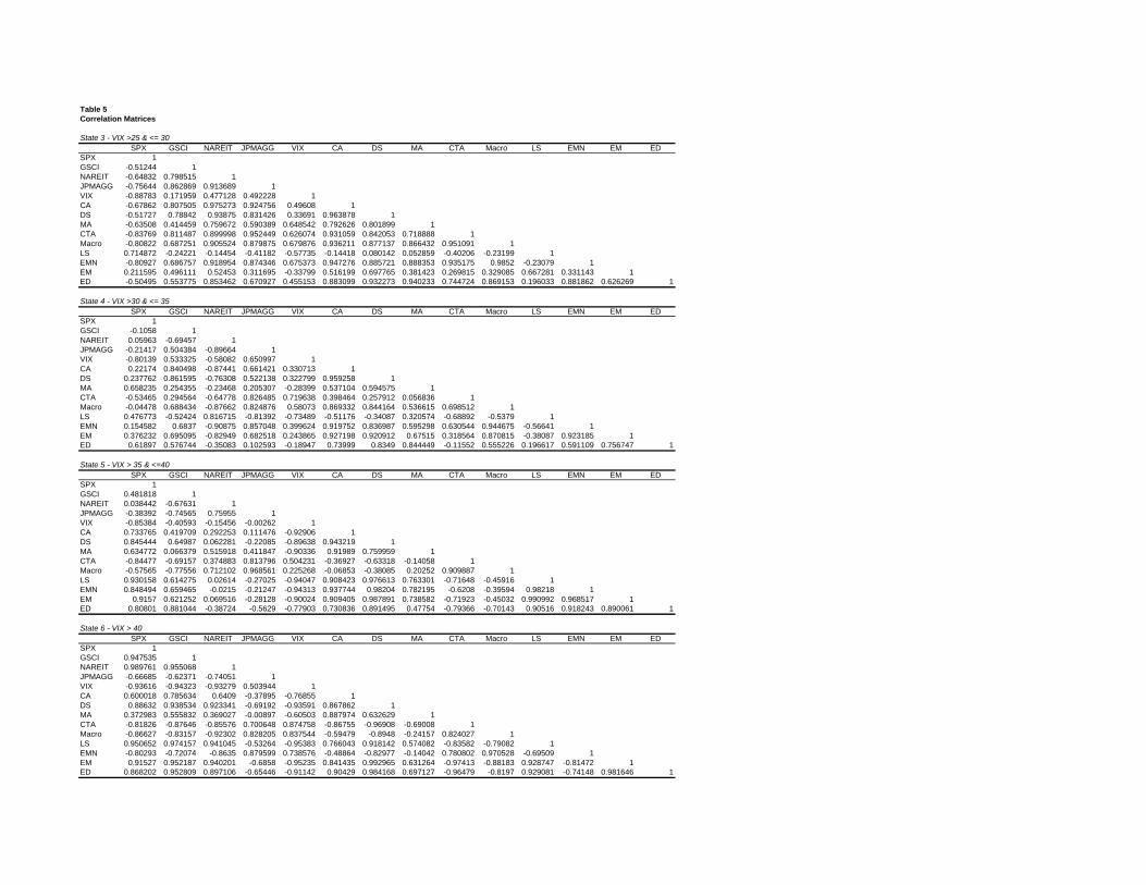
Table 5Correlation Matrices

State 3 - VIX >25 & <= 30SPX GSCI NAREIT JPMAGG VIX CA DS MA CTA Macro LS EMN EM ED

SPX 1GSCI -0.51244 1NAREIT -0.64832 0.798515 1JPMAGG -0.75644 0.862869 0.913689 1VIX -0.88783 0.171959 0.477128 0.492228 1CA -0.67862 0.807505 0.975273 0.924756 0.49608 1DS -0.51727 0.78842 0.93875 0.831426 0.33691 0.963878 1MA -0.63508 0.414459 0.759672 0.590389 0.648542 0.792626 0.801899 1CTA -0.83769 0.811487 0.899998 0.952449 0.626074 0.931059 0.842053 0.718888 1Macro -0.80822 0.687251 0.905524 0.879875 0.679876 0.936211 0.877137 0.866432 0.951091 1LS 0.714872 -0.24221 -0.14454 -0.41182 -0.57735 -0.14418 0.080142 0.052859 -0.40206 -0.23199 1EMN -0.80927 0.686757 0.918954 0.874346 0.675373 0.947276 0.885721 0.888353 0.935175 0.9852 -0.23079 1EM 0.211595 0.496111 0.52453 0.311695 -0.33799 0.516199 0.697765 0.381423 0.269815 0.329085 0.667281 0.331143 1ED -0.50495 0.553775 0.853462 0.670927 0.455153 0.883099 0.932273 0.940233 0.744724 0.869153 0.196033 0.881862 0.626269 1

State 4 - VIX >30 & <= 35SPX GSCI NAREIT JPMAGG VIX CA DS MA CTA Macro LS EMN EM ED

SPX 1GSCI -0.1058 1NAREIT 0.05963 -0.69457 1JPMAGG -0.21417 0.504384 -0.89664 1VIX -0.80139 0.533325 -0.58082 0.650997 1CA 0.22174 0.840498 -0.87441 0.661421 0.330713 1DS 0.237762 0.861595 -0.76308 0.522138 0.322799 0.959258 1MA 0.658235 0.254355 -0.23468 0.205307 -0.28399 0.537104 0.594575 1CTA -0.53465 0.294564 -0.64778 0.826485 0.719638 0.398464 0.257912 0.056836 1Macro -0.04478 0.688434 -0.87662 0.824876 0.58073 0.869332 0.844164 0.536615 0.698512 1LS 0.476773 -0.52424 0.816715 -0.81392 -0.73489 -0.51176 -0.34087 0.320574 -0.68892 -0.5379 1EMN 0.154582 0.6837 -0.90875 0.857048 0.399624 0.919752 0.836987 0.595298 0.630544 0.944675 -0.56641 1EM 0.376232 0.695095 -0.82949 0.682518 0.243865 0.927198 0.920912 0.67515 0.318564 0.870815 -0.38087 0.923185 1ED 0.61897 0.576744 -0.35083 0.102593 -0.18947 0.73999 0.8349 0.844449 -0.11552 0.555226 0.196617 0.591109 0.756747 1

State 5 - VIX > 35 & <=40SPX GSCI NAREIT JPMAGG VIX CA DS MA CTA Macro LS EMN EM ED

SPX 1GSCI 0.481818 1NAREIT 0.038442 -0.67631 1JPMAGG -0.38392 -0.74565 0.75955 1VIX -0.85384 -0.40593 -0.15456 -0.00262 1CA 0.733765 0.419709 0.292253 0.111476 -0.92906 1DS 0.845444 0.64987 0.062281 -0.22085 -0.89638 0.943219 1MA 0.634772 0.066379 0.515918 0.411847 -0.90336 0.91989 0.759959 1CTA -0.84477 -0.69157 0.374883 0.813796 0.504231 -0.36927 -0.63318 -0.14058 1Macro -0.57565 -0.77556 0.712102 0.968561 0.225268 -0.06853 -0.38085 0.20252 0.909887 1LS 0.930158 0.614275 0.02614 -0.27025 -0.94047 0.908423 0.976613 0.763301 -0.71648 -0.45916 1EMN 0.848494 0.659465 -0.0215 -0.21247 -0.94313 0.937744 0.98204 0.782195 -0.6208 -0.39594 0.98218 1EM 0.9157 0.621252 0.069516 -0.28128 -0.90024 0.909405 0.987891 0.738582 -0.71923 -0.45032 0.990992 0.968517 1ED 0.80801 0.881044 -0.38724 -0.5629 -0.77903 0.730836 0.891495 0.47754 -0.79366 -0.70143 0.90516 0.918243 0.890061 1

State 6 - VIX > 40SPX GSCI NAREIT JPMAGG VIX CA DS MA CTA Macro LS EMN EM ED

SPX 1GSCI 0.947535 1NAREIT 0.989761 0.955068 1JPMAGG -0.66685 -0.62371 -0.74051 1VIX -0.93616 -0.94323 -0.93279 0.503944 1CA 0.600018 0.785634 0.6409 -0.37895 -0.76855 1DS 0.88632 0.938534 0.923341 -0.69192 -0.93591 0.867862 1MA 0.372983 0.555832 0.369027 -0.00897 -0.60503 0.887974 0.632629 1CTA -0.81826 -0.87646 -0.85576 0.700648 0.874758 -0.86755 -0.96908 -0.69008 1Macro -0.86627 -0.83157 -0.92302 0.828205 0.837544 -0.59479 -0.8948 -0.24157 0.824027 1LS 0.950652 0.974157 0.941045 -0.53264 -0.95383 0.766043 0.918142 0.574082 -0.83582 -0.79082 1EMN -0.80293 -0.72074 -0.8635 0.879599 0.738576 -0.48864 -0.82977 -0.14042 0.780802 0.970528 -0.69509 1EM 0.91527 0.952187 0.940201 -0.6858 -0.95235 0.841435 0.992965 0.631264 -0.97413 -0.88183 0.928747 -0.81472 1ED 0.868202 0.952809 0.897106 -0.65446 -0.91142 0.90429 0.984168 0.697127 -0.96479 -0.8197 0.929081 -0.74148 0.981646 1

Table 6Transition probability matrix for VIX

Next day StateCurrent State 1 2 3 4 5 6

1 88.1% 11.0% 0.8% 0.0% 0.0% 0.0%2 24.5% 52.8% 13.2% 1.9% 3.8% 1.9%3 0.0% 37.0% 51.9% 11.1% 0.0% 0.0%4 0.0% 28.6% 28.6% 28.6% 14.3% 0.0%5 0.0% 0.0% 40.0% 20.0% 0.0% 40.0%6 0.0% 0.0% 14.3% 0.0% 28.6% 57.1%

Average Maximum % of all MonthsVIX State Duration Duration in State

1 8.4 45 54.6%2 1.8 6 24.1%3 2.1 5 12.5%4 1.4 2 3.2%5 1.0 1 2.3%6 2.3 3 3.2%

Notes:Based on monthly data. See Munenzon (2010) for the tables above based on daily data.

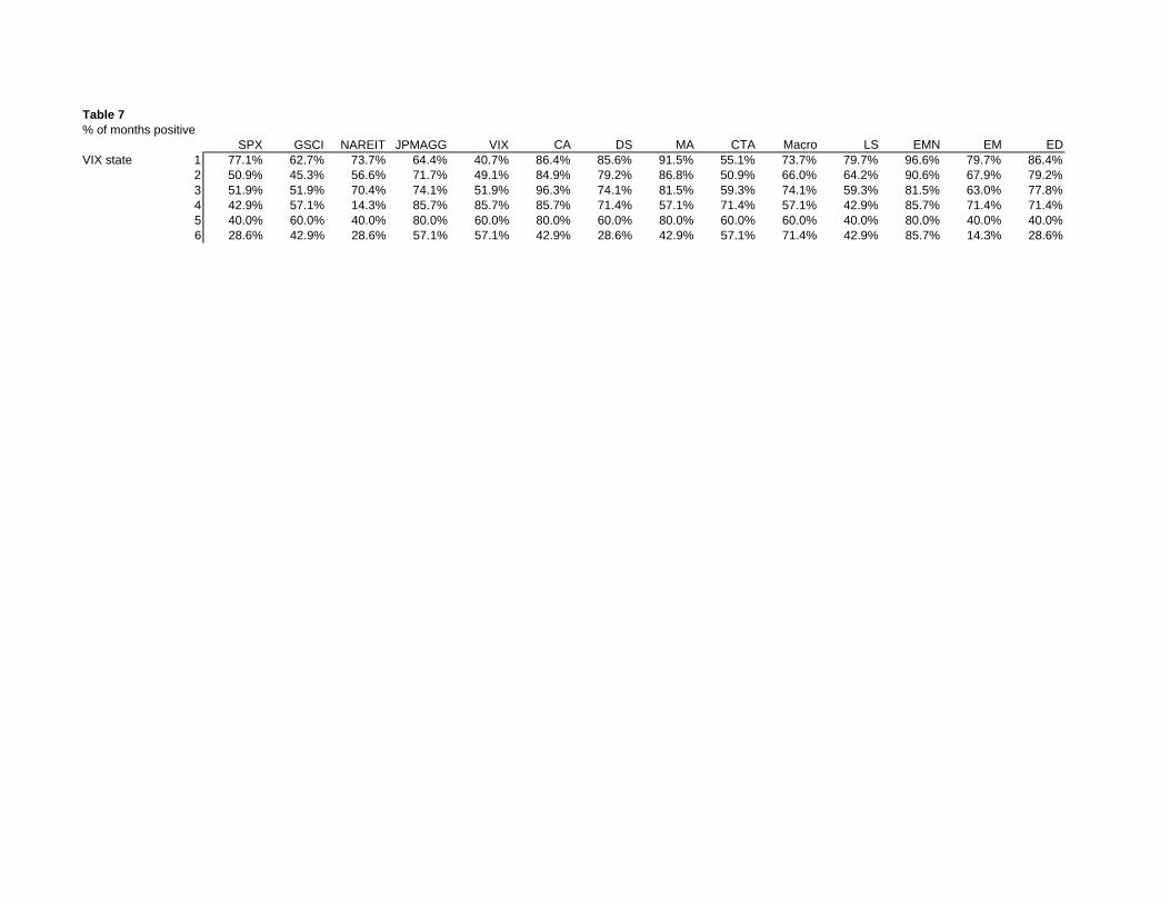
Table 7% of months positive

SPX GSCI NAREIT JPMAGG VIX CA DS MA CTA Macro LS EMN EM EDVIX state 1 77.1% 62.7% 73.7% 64.4% 40.7% 86.4% 85.6% 91.5% 55.1% 73.7% 79.7% 96.6% 79.7% 86.4%

2 50.9% 45.3% 56.6% 71.7% 49.1% 84.9% 79.2% 86.8% 50.9% 66.0% 64.2% 90.6% 67.9% 79.2%3 51.9% 51.9% 70.4% 74.1% 51.9% 96.3% 74.1% 81.5% 59.3% 74.1% 59.3% 81.5% 63.0% 77.8%4 42.9% 57.1% 14.3% 85.7% 85.7% 85.7% 71.4% 57.1% 71.4% 57.1% 42.9% 85.7% 71.4% 71.4%5 40.0% 60.0% 40.0% 80.0% 60.0% 80.0% 60.0% 80.0% 60.0% 60.0% 40.0% 80.0% 40.0% 40.0%6 28.6% 42.9% 28.6% 57.1% 57.1% 42.9% 28.6% 42.9% 57.1% 71.4% 42.9% 85.7% 14.3% 28.6%

20 Years of VIX: Fear, Greed and Implications for Alternative Investment Strategies

Documents

Transcript of 20 Years of VIX: Fear, Greed and Implications for Alternative Investment Strategies