20 Watersheds Erd
186
EPA/600/R-12/058A Watershed Modeling to Assess the Sensitivity of Streamflow, Nutrient, and Sediment Loads to Potential Climate Change and Urban Development in 20 U.S. Watersheds NOTICE THIS DOCUMENT IS A DRAFT. This document is distributed solely for the purpose of pre- dissemination peer review under applicable information quality guidelines. It has not been formally disseminated by EPA. It does not represent and should not be construed to represent any Agency determination or policy. Mention of trade names or commercial products does not constitute endorsement or recommendation for use National Center for Environmental Assessment Office of Research and Development U.S. Environmental Protection Agency Washington, DC 20460 i
-
Upload
quantanglement -
Category
Documents
-
view
226 -
download
0
Transcript of 20 Watersheds Erd
8/13/2019 20 Watersheds Erd
http://slidepdf.com/reader/full/20-watersheds-erd 1/186
EPA/600/R-12/058A
Watershed Modeling to Assess the Sensitivity of Streamflow, Nutrient, and Sediment Loads to Potential Climate Change and
Urban Development in 20 U.S. Watersheds
NOTICE THIS DOCUMENT IS A DRAFT. This document is distributed solely for the purpose of pre- dissemination peer review under applicable information quality guidelines. It has not been
formally disseminated by EPA. It does not represent and should not be construed to represent any Agency determination or policy. Mention of trade names or commercial products does not constitute endorsement or recommendation for use
National Center for Environmental Assessment Office of Research and Development
U.S. Environmental Protection Agency Washington, DC 20460
i

8/13/2019 20 Watersheds Erd
http://slidepdf.com/reader/full/20-watersheds-erd 2/186
DISCLAIMER This document is distributed solely for the purpose of pre-dissemination peer review under applicableinformation quality guidelines. It has not been formally disseminated by EPA. It does not represent
and should not be construed to represent any Agency determination or policy. Mention of trade names
or commercial products does not constitute endorsement or recommendation for use.
Preferred Citation:

8/13/2019 20 Watersheds Erd
http://slidepdf.com/reader/full/20-watersheds-erd 3/186
FOREWORD
iii
8/13/2019 20 Watersheds Erd
http://slidepdf.com/reader/full/20-watersheds-erd 4/186
AUTHORS AND REVIEWERS
The National Center for Environmental Assessment (NCEA), Office of Research and Development,was responsible for preparing this External Review Draft report. An earlier draft report was prepared
by Tetra Tech Inc., under EPA Contract EP-C-05-061.
AUTHORS
Tetra Tech Inc. Jonathan Butcher, Andrew Parker, Saumya Sarkar, Scott Job, Mustafa Faizullabhoy, Peter Cada, Jeremy Wyss Texas A&M University
Raghavan Srinivasan, Pushpa Tuppad, Deb Debjani
Aqua Terra Consultants
Anthony Donigian, John Imhoff, Jack Kittle, Brian Bicknell, Paul Hummel, Paul Duda
U.S. Environmental Protection Agency, Office of Research and Development Thomas Johnson, Chris Weaver, Meredith Warren (ORISE Fellow), Daniel Nover (AAAS Fellow)
REVIEWERS
Comments on a previous draft of this report were provided by EPA staff David Bylsma, Chris Clark,Steve Klein, and Chris Weaver.
ACKNOWLEDGEMENTS
The authors acknowledge and thank for their hard work the entire project team at Tetra Tech (Tt),
Texas A&M University (TAMU), AQUA TERRA (AT), Stratus Consulting, and FTN Associates. We
also thank Seth McGinnis of the National Center for Atmospheric Research (NCAR) for processing the NARCCAP output into change statistics for use in the watershed modeling. NCAR is supported by the
National Science Foundation. We acknowledge the modeling groups, the Program for Climate Model
Diagnosis and Intercomparison (PCMDI) and the WCRP's Working Group on Coupled Modeling
(WGCM) for their roles in making available the WCRP CMIP3 multi-model dataset. Support of thisdataset is provided by the Office of Science, U.S. Department of Energy.
iv
8/13/2019 20 Watersheds Erd
http://slidepdf.com/reader/full/20-watersheds-erd 5/186
TABLE OF CONTENTS
1. EXECUTIVE SUMMARY .................................................................................................1 2. INTRODUCTION ...............................................................................................................4
2.1. About this Report .....................................................................................................6 3. STUDY AREAS ..................................................................................................................7
3.1. Description of Study Areas ....................................................................................12 3.1.1. Apalachicola-Chattahoochee-Flint (ACF) River Basin (Pilot) ............................................. 12 3.1.2. Minnesota River Basin (Pilot) ............................................................................................ 14 3.1.3. Salt/Verde/San Pedro River Basin (Pilot) .......................................................................... 16 3.1.4. Susquehanna River Basin (Pilot) ....................................................................................... 19 3.1.5. Willamette River Basin (Pilot) ........................................................................................... 21 3.1.6. Coastal Southern California basins ................................................................................... 23 3.1.7. Cook Inlet basin ................................................................................................................. 25 3.1.8. Georgia-Florida Coastal basins .......................................................................................... 27 3.1.9. Upper Illinois River basin................................................................................................... 29 3.1.10. Lake Erie Drainages ......................................................................................................... 31 3.1.11. Lake Pontchartrain basin................................................................................................. 32 3.1.12. Loup/Elkhorn River basin ................................................................................................ 35 3.1.13. Tar/Neuse River basins ................................................................................................... 36 3.1.14. New England Coastal basins............................................................................................ 37 3.1.15. Powder/Tongue River basin ............................................................................................ 40 3.1.16. Rio Grande Valley basin .................................................................................................. 42 3.1.17. Sacramento River basin................................................................................................... 44 3.1.18. South Platte River basin .................................................................................................. 46 3.1.19. Trinity River basin ............................................................................................................ 48 3.1.20. Upper Colorado River basins ........................................................................................... 50
4. Modeling Approach ...........................................................................................................52 4.1. Model Background ................................................................................................53
4.1.1. HSPF .................................................................................................................................. 53 4.1.2. SWAT ................................................................................................................................. 54 4.2. Model Setup ...........................................................................................................55 4.2.1. SWAT Setup Process ......................................................................................................... 56 4.2.2. HSPF Setup Process ........................................................................................................... 58 4.2.3. Watershed Data Sources ................................................................................................... 58 4.2.4. Weather Representation................................................................................................... 64
4.3. Model simulation Endpoints ..................................................................................66 4.4. Model Calibration and Validation .........................................................................69
4.4.1. Hydrology .......................................................................................................................... 69 4.4.2. Water Quality .................................................................................................................... 72 4.4.3. Accuracy of the Watershed Models .................................................................................. 73
5. Climate change and urban development Scenarios ...........................................................77
5.1. Climate Change Scenarios .....................................................................................77 5.1.1. North American Regional Climate Change Assessment Program (NARCCAP)
Scenarios ........................................................................................................................ 80 5.1.2. Bias-Corrected and Spatially Downscaled (BCSD) Scenarios ............................................ 80 5.1.3. Global Climate Models (GCMs) without Downscaling ...................................................... 81 5.1.4. Translation of Climate Model Projections to Meteorological Model Inputs .................... 81
5.2. Urban Development Scenarios ..............................................................................91 5.2.1. Land Use Scenarios ........................................................................................................... 91
v
8/13/2019 20 Watersheds Erd
http://slidepdf.com/reader/full/20-watersheds-erd 6/186
5.2.2. Translating ICLUS Land Use Projections to Watershed Model Inputs .............................. 91
6. Results in Pilot Watersheds: Sensitivity to Different Methodological Choices ................95 6.1. Comparison of Watershed Models ........................................................................95
6.1.1. Influence of Calibration Strategies .................................................................................... 96 6.1.2. Comparison of Model Calibration and Validation Performance ....................................... 97 6.1.3. Consistency of Simulated Changes Using SWAT and HSPF ............................................. 101 6.1.4. Watershed Model Response to Increased Atmospheric CO2 ......................................... 105 6.1.5. Selection of Watershed Model for Use in All Study Areas .............................................. 108
6.2. Effects of Different Methods of Downscaling of Climate Change Projections ..109 6.2.1. “Degraded” NARCCAP Climate Scenarios ....................................................................... 109 6.2.2. Comparison of Downscaling Approaches ....................................................................... 111
7. Results in all 20 watersheds: Regional Sensitivity to Climate Change and Urban Development ....................................................................................................................117 7.1. Sensitivity to Climate Change Scenarios .............................................................118 7.2. Sensitivity to Urban and Residential Development Scenarios ............................127 7.3. Relative effects of climate change and Urban Development Scenarios ..............129 7.4. Sensitivity to Combined Climate Change and Urban Development Scenarios ...132 7.5. Sensitivity of Study Area Water Balance Indicators ...........................................151
8. Modeling Uncertainty and Assumptions .........................................................................157 8.1. Model Calibration ................................................................................................159 8.2. Watershed Model .................................................................................................159
9. Summary and Conclusions ..............................................................................................162 References .................................................................................................................................... 165
vi
8/13/2019 20 Watersheds Erd
http://slidepdf.com/reader/full/20-watersheds-erd 7/186
LIST OF APPENDICES
Appendix A. SWAT Model Setup ProcessAppendix B. Quality Assurance Project Plan (QAPP)
Appendix C. Modeling the Impacts of Climate and Landuse Change: Climate Change and the
Frequency and Intensity of Precipitation Events - Memo
Appendix D. Model Configuration, Calibration and Validation for the ACF River BasinAppendix E. Model Configuration, Calibration and Validation for the Central Arizona Basins
Appendix F. Model Configuration, Calibration and Validation for the Susquehanna River Basin
Appendix G. Model Configuration, Calibration and Validation for the Minnesota River BasinAppendix H. Model Configuration, Calibration and Validation for the Willamette River Basin
Appendix I. Model Configuration, Calibration and Validation for the Acadian-Pontchartrain Drainages
Appendix J. Model Configuration, Calibration and Validation for the Albemarle-Pamlico River BasinsAppendix K . Model Configuration, Calibration and Validation for the Central Nebraska Basins
Appendix L. Model Configuration, Calibration and Validation for the Cook Inlet Basin
Appendix M. Model Configuration, Calibration and Validation for the Georgia-Florida Coastal Basins
Appendix N. Model Configuration, Calibration and Validation for the Illinois River Basin
Appendix O. Model Configuration, Calibration and Validation for the Lake Erie-Lake St. Clair BasinsAppendix P. Model Configuration, Calibration and Validation for the New England Coastal Basins
Appendix Q. Model Configuration, Calibration and Validation for the Rio Grande Valley BasinAppendix R . Model Configuration, Calibration and Validation for the Sacramento River Basin
Appendix S. Model Configuration, Calibration and Validation for the Coastal Southern California
BasinsAppendix T. Model Configuration, Calibration and Validation for the South Platte River Basin
Appendix U. Model Configuration, Calibration and Validation for the Trinity River Basin
Appendix V. Model Configuration, Calibration and Validation for the Upper Colorado River Basin
Appendix W. Model Configuration, Calibration and Validation for the Yellowstone River BasinAppendix X. Scenario Results for the Five Pilot Watersheds
Appendix Y. Scenario Results for the 15 Non-pilot WatershedsAppendix Z. Overview of Climate Scenario Monthly Temperature, Precipitation, and Potential
Evapotranspiration.
vii
8/13/2019 20 Watersheds Erd
http://slidepdf.com/reader/full/20-watersheds-erd 8/186
LIST OF TABLES
Table 1. Site names, ID codes, and state locations of the 20 study areas. ................................................ 7 Table 2. Summary of the 20 study areas. ................................................................................................ 10 Table 3. Current (2001) land use and land cover in the 20 study areas. ................................................. 11 Table 4. Regrouping of the NLCD 2001 land-use classes for the HSPF and SWAT models. ............... 60 Table 5. Calculated fraction impervious cover by developed land class for each study area. ............... 61 Table 6. Characteristics of soil hydrologic groups. ................................................................................ 61
Table 7. Weather station statistics for the 20 study areas (1971-2000). ................................................. 64 Table 8. Summary of streamflow and water quality endpoints. ............................................................. 68 Table 9. Performance targets for hydrologic simulation (magnitude of annual and seasonal relative
mean error). ............................................................................................................................................. 70 Table 10. Key hydrology calibration parameters for HSPF. .................................................................. 72 Table 11. Key hydrology calibration parameters for SWAT. ................................................................ 72 Table 12. Summary of SWAT model fit for initial calibration site (20 Watersheds). ........................... 75 Table 13. Summary of HSPF model fit for initial calibration sites (5 Pilot Watersheds) ...................... 76 Table 14. Climate models and source of model data used to develop climate change scenarios. .......... 79 Table 15. Climate change data available from each source used to develop scenarios. ......................... 82 Table 16. SWAT weather generator parameters and adjustments applied for scenarios. ...................... 88 Table 17. Comparison of PET estimation between different downscaling approaches ......................... 90 Table 18. ICLUS projected changes in developed land within different imperviousness classes by 2050. ....................................................................................................................................................... 93 Table 19. Percent error in simulated total flow volume for 10-year calibration and validation periods.98 Table 20. Nash Sutcliffe coefficient of model fit efficiency ( E ) for daily flow predictions, 10-year calibration and validation periods. .......................................................................................................... 98 Table 21. Statistical comparison of HSPF and SWAT outputs at downstream station for the five pilot sites across all climate scenarios ........................................................................................................... 103 Table 22. Effects of omitting simulated auxiliary meteorological time series on Penman-Monteith
reference crop PET estimates for “degraded” climate scenarios .......................................................... 110 Table 23. Summary of SWAT-simulated total streamflow in the five pilot study areas for scenarios representing different methods of downscaling. ................................................................................... 111 Table 24. Summary of SWAT-simulated streamflow and water quality in the Minnesota River study area for scenarios representing different methods of downscaling. ..................................................... 112 Table 25. Range of simulated percent changes for NARCCAP climate scenarios; SWAT simulation with ICLUS landuse for 2041 – 2070 (percent change in annual flow and load). ............................... 116 Table 26. Downstream stations where simulation results are presented. ............................................. 117 Table 27. Simulated total flow volume (climate scenarios only; percent relative to current conditions) for selected downstream stations. ......................................................................................................... 119 Table 28. Simulated 7-day low flow (climate scenarios only; percent relative to current conditions) for selected downstream stations. ............................................................................................................... 120 Table 29. Simulated 100-year peak flow (log-Pearson III; climate scenarios only; percent relative to current conditions) for selected downstream stations. .......................................................................... 121 Table 30. Simulated changes in the number of days to flow centroid (climate scenarios only; relative tocurrent conditions) for selected downstream stations. .......................................................................... 122 Table 31. Simulated Richards-Baker flashiness index (climate scenarios only; percent relative to
current conditions) for selected downstream stations. .......................................................................... 123 Table 32. Simulated total suspended solids load (climate scenarios only; percent relative to current conditions) for selected downstream stations. ...................................................................................... 124
viii
8/13/2019 20 Watersheds Erd
http://slidepdf.com/reader/full/20-watersheds-erd 9/186
Table 33. Simulated total phosphorus load (climate scenarios only; percent relative to current conditions) for selected downstream stations. ...................................................................................... 125 Table 34. Simulated total nitrogen load (climate scenarios only; percent relative to current conditions) for selected downstream stations. ......................................................................................................... 126 Table 35. Simulated response to projected 2050 changes in urban and residential development (percent or days relative to current conditions) for selected downstream stations. ............................................ 128 Table 36. Simulated range of responses of mean annual flow to mid-21
st
century climate and land usechange at the HUC8 and larger scale. ................................................................................................... 131 Table 37. Simulated total flow volume (climate and land use change scenarios; percent relative to current conditions) for selected downstream stations. .......................................................................... 134 Table 38. Simulated 7-day low flow (climate and land use change scenarios; percent relative to current conditions) for selected downstream stations. ...................................................................................... 136 Table 39. Simulated 100-year peak flow (log-Pearson III; climate and land use change scenarios; percent relative to current conditions) for selected downstream stations. ............................................ 138 Table 40. Simulated change in the number of days to flow centroid (climate and land use change scenarios; relative to current conditions) for selected downstream stations. ........................................ 140 Table 41. Simulated Richards-Baker flashiness index (climate and land use change scenarios; percent relative to current conditions) for selected downstream stations. ......................................................... 142 Table 42. Simulated total suspended solids load (climate and land use change scenarios; percent relative to current conditions) for selected downstream stations. ......................................................... 144 Table 43. Simulated total phosphorus load (climate and land use change scenarios; percent relative to
current conditions) for selected downstream stations. .......................................................................... 146 Table 44. Simulated total nitrogen load (climate and land use change scenarios; percent relative tocurrent conditions) for selected downstream stations. .......................................................................... 148 Table 45. Coefficient of Variation of SWAT-simulated changes in streamflow for each study area in response to the six NARCCAP climate change scenarios for selected downstream stations. ............. 150 Table 46. Coefficient of variation of SWAT-simulated changes in streamflow for each NARCCAP climate scenario for selected downstream stations. .............................................................................. 151 Table 47. Simulated percent changes in water balance statistics for study areas (NARCCAP climatewith land use change scenarios; median percent change relative to current conditions). .................... 152
ix
8/13/2019 20 Watersheds Erd
http://slidepdf.com/reader/full/20-watersheds-erd 10/186
LIST OF FIGURES
Figure 1. Locations of the 20 study areas. ................................................................................................ 9 Figure 2. Apalachicola-Chattahoochee-Flint (ACF) River basin. .......................................................... 13 Figure 3. Minnesota River watershed. .................................................................................................... 15 Figure 4. The Central Arizona basins – Verde and Salt River sections. ................................................ 17 Figure 5. The Central Arizona basins – San Pedro River section. ......................................................... 18 Figure 6. Susquehanna River watershed. ................................................................................................ 20 Figure 7. Willamette River watershed. ................................................................................................... 22 Figure 8. Coastal Southern California River basins model area. ............................................................ 24 Figure 9. Cook Inlet basin model area. ................................................................................................... 26 Figure 10. Georgia-Florida Coastal Plain basins model area. ................................................................ 28 Figure 11. Illinois River basin model area.............................................................................................. 30 Figure 12. Lake Erie drainages model area. ........................................................................................... 32 Figure 13. Lake Pontchartrain basin model area. ................................................................................... 34 Figure 14. Loup and Elkhorn River basins model area. ......................................................................... 36 Figure 15. Tar/Neuse River basin model area. ....................................................................................... 37 Figure 16. New England Coastal basins model area. ............................................................................. 39 Figure 17. Tongue and Powder River basins model area. ...................................................................... 41 Figure 18. Rio Grande Valley basin model area. .................................................................................... 43 Figure 19. Sacramento River basin model area. ..................................................................................... 45 Figure 20. South Platte River basin model area. .................................................................................... 47 Figure 21. Trinity River basin model area. ............................................................................................. 49 Figure 22. Upper Colorado River basin model area. .............................................................................. 51 Figure 23. Average monthly precipitation in the 20 study areas (1971-2000). ...................................... 65 Figure 24. Average monthly temperature in the 20 study areas (1971-2000). ....................................... 65 Figure 25. Comparison of model calibration fit to flow for the calibration initial site. ......................... 99 Figure 26. Sensitivity of model fit for total flow volume to temporal change. ...................................... 99 Figure 27. Sensitivity of model fit for flow to spatial change. ............................................................. 100 Figure 28. Comparison of baseline adjusted model fit efficiency for total suspended solids monthly loads for calibration site (left) and downstream site (right). ................................................................ 100 Figure 29. Comparison of baseline adjusted model fit efficiency for total phosphorus monthly loads for calibration site (left) and downstream site (right). ................................................................................ 101 Figure 30. Comparison of baseline adjusted model fit efficiency for total nitrogen monthly loads for calibration site (left) and downstream site (right). ................................................................................ 101 Figure 31. SWAT and HSPF simulated changes in total flow in pilot watersheds (expressed relative to
current conditions). ............................................................................................................................... 102 Figure 32. SWAT and HSPF simulated changes in TSS in pilot watersheds (expressed relative to
current conditions). ............................................................................................................................... 104 Figure 33. SWAT and HSPF simulated changes in total nitrogen load in pilot watersheds (expressed
relative to current conditions). .............................................................................................................. 105 Figure 34. Simulated effect of changes in atmospheric CO2 concentration on selected streamflow and water quality endpoints using SWAT. .................................................................................................. 107 Figure 35. Consistency in SWAT model predictions of mean annual flow with downscaled(NARCCAP, BCSD) and GCM projections of the GFDL GCM ......................................................... 114 Figure 36. Consistency in SWAT model predictions of mean annual flow with downscaled
(NARCCAP, BCSD) and GCM projections of the CGCM3 GCM...................................................... 114 Figure 37. Comparison of simulated responses of mean annual flow to urban development and climate change scenarios – HSPF model. .......................................................................................................... 130
x
8/13/2019 20 Watersheds Erd
http://slidepdf.com/reader/full/20-watersheds-erd 11/186
Figure 38. Simulated total future flow volume relative to current conditions (NARCCAP climate scenarios with urban development) for selected stations. .................................................................... 135 Figure 40. Simulated 7-day low flow relative to current conditions (NARCCAP climate scenarios with urban development) for selected downstream stations ......................................................................... 137 Figure 42. Simulated 100-yr peak flow relative to current conditions (NARCCAP climate scenarios with urban development) for selected downstream stations ................................................................. 139 Figure 44. Simulated change in days to flow centroid relative to current conditions (NARCCAP
climate scenarios with urban development) for selected downstream stations .................................... 141 Figure 46. Simulated Richards-Baker flashiness index relative to current conditions (NARCCAP climate scenarios with urban development) for selected downstream stations .................................... 143 Figure 48. Simulated total suspended solids load relative to current conditions (NARCCAP climate scenarios with urban development) for selected downstream stations. ................................................ 145 Figure 50. Simulated total phosphorus load relative to current conditions (NARCCAP climate scenarios with urban development) for selected downstream stations. ................................................ 147 Figure 52. Simulated total nitrogen load relative to current conditions (NARCCAP climate scenarios with urban development) for selected downstream stations. ................................................................ 149 Figure 54. Median simulated percent changes in watershed Dryness Ratio for 6 NARCCAP scenarios relative to current conditions (median of NARCCAP climate scenarios with urban development). ... 153 Figure 55. Median simulated percent changes in watershed low flow sensitivity for 6 NARCCAP scenarios relative to current conditions (median of NARCCAP climate scenarios with urban
development). ....................................................................................................................................... 153 Figure 56. Median simulated percent changes in watershed surface runoff fraction for 6 NARCCAP scenarios relative to current conditions (median of NARCCAP climate scenarios with urbandevelopment). ....................................................................................................................................... 154 Figure 57. Median simulated percent changes in watershed snowmelt fraction for 6 NARCCAP scenarios relative to current conditions (median of NARCCAP climate scenarios with urban development). ....................................................................................................................................... 154 Figure 58. Median simulated percent changes in watershed deep recharge for 6 NARCCAP scenarios relative to current conditions (median of NARCCAP climate scenarios with urban development). ... 155
xi
8/13/2019 20 Watersheds Erd
http://slidepdf.com/reader/full/20-watersheds-erd 12/186
1
234
5
67
8
9
1011
12
1314
15
16
1718
19
2021
22
2324
25
2627
28
2930
31
32
3334
35
36
LIST OF ABBREVIATIONS
AET actual evapotranspirationBASINS Better Assessment Science Integrating Point and Non-point Sources
CAT Climate Assessment Tool
cfs cubic feet per secondCMIP3 Coupled Model Intercomparison Project Phase 3
cms cubic meters per second
E Nash-Sutcliffe model efficiency coefficient
ET evapotranspirationGCM global climate model
GIS geographic information system
HRU hydrologic response unitHSPF Hydrologic Simulation Program-FORTRAN
HUC hydrologic unit code
IPCC Intergovernmental Panel on Climate Change
NARCCAP North American Regional Climate Change Assessment Program NCAR National Center for Atmospheric Research
NCDC National Climatic Data Center
NLCD National Land Cover Data NOAA National Oceanic and Atmospheric Administration
NRCS Natural Resource Conservation Service
PET potential evapotranspirationPRISM Parameter-elevation Regressions on Independent Slopes Model
R 2
coefficient of determination
RCM regional climate modelRMSE root mean square error
STATSGO State Soil Geographic Database
SWAT Soil Water Assessment ToolTN total nitrogen
TP total phosphorus
TSS total suspended solids
U.S. EPA U.S. Environmental Protection AgencyUSDA U.S. Department of Agriculture
USGS U.S. Geologic Survey
0
8/13/2019 20 Watersheds Erd
http://slidepdf.com/reader/full/20-watersheds-erd 13/186
5
10
15
20
25
30
35
40
45
1 1. EXECUTIVE SUMMARY
There is growing concern about the potential effects of climate change on water resources.The 2007 Fourth Assessment Report of the Intergovernmental Panel on Climate Change (IPCC)
states that warming of the climate system is now unequivocal (IPCC, 2007). Regionally variable
changes in the amount and intensity of precipitation have also been observed in much of the U.S.(Groisman et al., 2005). Climate modeling experiments suggest these trends will continue
throughout the 21st century, with continued warming accompanied by a general intensification
of the global hydrologic cycle (IPCC, 2007; Karl et al., 2009). Water and watershed systems are
highly sensitive to climate. In many areas, climate change is expected to exacerbate currentstresses on water resources from population growth and economic and land-use change,
including urbanization (IPCC, 2007). Responding to this challenge requires an improved
understanding of how we are vulnerable, and the development of strategies for managing climaterisk.
This report describes watershed modeling in 20 large, U.S. drainage basins (6,000-27,000 mi2) to
characterize the sensitivity of U.S. streamflow, nutrient (N and P) loading, and sediment loading
to a range of potential mid-21st century climate futures, to assess the potential interaction of
climate change and urbanization in these basins, and to improve our understanding ofmethodological challenges associated with integrating existing tools (e.g., climate models,
downscaling approaches, and watershed models) and datasets to address these scientific
questions. Study areas were selected to represent a range of geographic, hydroclimatic,
physiographic, and land use conditions together with practical considerations such as theavailability of data to calibrate and validate watershed models. Climate change scenarios are
based on mid-21st century climate model projections downscaled with regional climate models
(RCMs) from the North American Regional Climate Change Assessment Program (NARCCAP)and the bias-corrected and spatially downscaled (BCSD) data set described by Maurer et al.
(2007). Urban and residential development scenarios are based on EPA’s national-scaleIntegrated Climate and Land Use Scenarios (ICLUS) project (U.S. EPA, 2009d). Watershed
modeling was conducted using the Hydrologic Simulation Program-FORTRAN (HSPF) and Soil
and Water Assessment Tool (SWAT) watershed models.
Climate change scenarios based on global climate model (GCM) simulations in the NARCCAP
and BCSD datasets show a continued general warming trend throughout the nation over the nextcentury, although the magnitude of the warming varies from place to place. Wetter winters and
earlier snowmelt are likely in many of the northern and higher elevation watersheds. Changes in
other aspects of local climate such as the timing and intensity of precipitation show greater
variability and uncertainty. ICLUS urban and residential development scenarios show continued
growth in urban and developed land over the next century throughout the nation with mostgrowth occurring in and around existing urban areas. Model simulations of watershed response
to these changes provide a national scale perspective on the range of potential changes instreamflow and water quality in different regions of the nation. Simulations evaluating the
variability in watershed response using different approaches for downscaling climate data and
different watershed models provide guidance on the use of existing models and datasets forassessing climate change impacts. Key findings are summarized below.
23
4
6
7
8
9
11
1213
14
16
17
1819
21
2223
24
26
2728
29
31
32
3334
36
37
3839
41
42
4344
1
8/13/2019 20 Watersheds Erd
http://slidepdf.com/reader/full/20-watersheds-erd 14/186
1
23
4
5
67
89
1011
1213
14
1516
1718
1920
21
2223
24
2526
27
282930
3132
33
3435
36
3738
394041
42
43
4445
46
2
There is a high degree regional variability in the model simulated responses of different
streamflow and water quality endpoints to a range of potential mid-21st century climatic
conditions throughout the nation. Comparison of watershed simulations in all 20 study areas
for the 2041-2070 time horizon suggests the following hydrologic changes may occur:
Potential flow volume decreases in the Rockies and interior southwest, and increases inthe east and southeast coasts.
Higher peak flows will increase erosion and sediment transport; loads of nitrogen and phosphorus are also likely to increase in many watersheds.
Streamflow responses are determined by the interaction of changes in precipitation andevapotranspiration; nutrient and sediment loads are generally correlated with changes in
hydrology.
The simulated responses of streamflow and water quality endpoints to climate change
scenarios based on different climate models and downscaling methodologies in many cases
span a wide range and sometimes do not agree in the direction of change. The ultimate
significance of any given simulation of future change will depend on local context, including thehistorical range of variability, thresholds and management targets, management options, and
interaction with other stressors. The simulation results in this study do, however, clearly illustratethat the potential streamflow and water quality response in many areas could be large. Given
these uncertainties, successful climate change adaptation strategies will likely need to encompass
practices and decisions to reduce vulnerabilities and risk across a range of potential futureclimatic conditions.
Simulated responses to urban development scenarios were small relative to those resulting
from climate change in this study. This is likely due to the relatively small changes in
developed lands as a percent of total watershed area at the large spatial scale of watersheds in
this study. At the finest spatial scale evaluated in this study, that of an 8 digit HUC, urban andresidential growth scenarios represented changes on the order of <1 to about 12 percent of totalwatershed area. As would be expected, such small changes in development did not have a large
effect on streamflow or water quality. It is well documented, however, that urban and residentialdevelopment at higher levels can have significant impacts on streamflow and water quality. At
smaller spatial scales where changes in developed lands represent a larger percentage of
watershed area the effects of urbanization are likely to be greater. The scale at whichurbanization effects may become comparable to the effects of a changing climate is uncertain.
Simulation results are sensitive to methodological choices such as different approaches for
downscaling global climate change simulations and use of different watershed models.
Watershed simulations in this study suggest that the variability in watershed response resultingfrom a single GCM downscaled using different RCM models can be of the same order ofmagnitude as the ensemble variability between the different GCMs evaluated. Watershed
simulations using different models with different structures and methods for representing
watershed processes (HSPF and SWAT in this study) also resulted in increased variability of
outcomes. SWAT simulations accounting for the influence of increased atmospheric CO2 onevapotranspiration significantly affected results. One notable insight from these results is that, in
many watersheds, increases in precipitation amount and/or intensity, urban development, and
8/13/2019 20 Watersheds Erd
http://slidepdf.com/reader/full/20-watersheds-erd 15/186
1
23
4
5
67
8
9
10
1112
13
14
15
16
1718
19
2021
22
atmospheric CO2 can have similar or additive effects on streamflow and pollutant loading, e.g., a
more flashy runoff response with higher high flows and lower low flows.
Next steps. This study is a significant contribution to our growing understanding of the complex
and context dependent relationships between climate change, urban development, and water
throughout the nation. It is only an incremental step, however, towards fully addressing thesequestions. Limitations of model simulations in this study include:
Several of the study areas are complex, highly managed systems; all infrastructure and
operational aspects of water management are not represented in full detail.
Changes in agricultural practices, water demand, other human responses, and naturalecosystem changes such as the prevalence of forest fire or plant disease that will
influence streamflow and water quality are not considered in this study.
Watershed simulations are constrained by the specific climate change and urban
development scenarios used as input to watershed models; scenarios represent a plausible
range but are not comprehensive of all possible futures.
The models used in this study each require calibration, and the calibration processinevitably introduces potential biases related to the approach taken and individual
modeler choices.
Further study is required to fully address the implications of these and other questions.
3
8/13/2019 20 Watersheds Erd
http://slidepdf.com/reader/full/20-watersheds-erd 16/186
5
10
15
20
25
30
35
40
45
1 2. INTRODUCTION
It is now generally accepted that human activities including the combustion of fossil fuels and
land-use change have resulted, and will continue to result in long-term changes in climate (IPCC,2007; Karl et al., 2009). The 2007 Fourth Assessment Report of the Intergovernmental Panel on
Climate Change (IPCC) states that “warming of the climate system is unequivocal, as is now
evident from observations of increases in global average air and ocean temperatures, widespreadmelting of snow and ice and rising global average sea level” (IPCC, 2007). Regionally variable
changes in the amount and intensity of precipitation have also been observed in much of the U.S.
(Groisman et al., 2005). Climate modeling experiments suggest these trends will continuethroughout the 21
stcentury, with continued warming accompanied by a general intensification of
the global hydrologic cycle (IPCC, 2007; Karl et al., 2009). While significant uncertainty
remains, particularly with respect to precipitation changes at local and regional spatial scales, the
presence of long-term trends in the record suggests many parts of the U.S. could experiencefuture climatic conditions unprecedented in recent history. Such changes challenge the
assumption of climate stationarity that has provided the foundation for water management for
decades (e.g., Milly et al., 2008).
Water and watershed systems are highly sensitive to changes in climate. Air temperatures are
anticipated to increase throughout most of the nation. Warmer air temperatures can result inincreased evaporation from soils and surface water; changes in the dynamics of snowfall and
snowmelt affecting runoff; changes in land cover affecting pollutant loading and watershed
biogeochemical cycling. Warming air temperatures are also likely to cause warming of rivers andlakes with cascading effects on individual species, community composition, and water quality.
Such changes together with decreased precipitation could contribute to more regions
experiencing drought. Precipitation changes are more regionally variable and not as well
understood. Generally, runoff is projected increase at higher latitudes and in some wet tropical
areas, and decrease over dry and semi-arid regions at mid-latitudes due to decreases in rainfalland higher rates of evapotranspiration (IPCC, 2007). Northern and mountainous areas that
receive snow in the winter are likely to see increased precipitation occurring as rain versus snow.In addition, most regions of the U.S. are expected to experience increasing intensity of
precipitation events, i.e., the fraction of total precipitation occurring in large magnitude events,
due to a warming induced general intensification of the global hydrologic cycle. Precipitationchanges can result in hydrologic effects including changes in amount and seasonal timing of
streamflow, changes in soil moisture and groundwater recharge, changes in land cover watershed
biogeochemical cycling, changes in non-point pollutant loading to water bodies, and increased
demands on water infrastructure including urban stormwater and other engineered systems.Regions exposed to increased storm intensity could experience increased coastal and inland
flooding.
Climate change is expected to exacerbate current stresses on water resources from population
growth and economic and land-use change, including urbanization (IPCC, 2007). Some systems
and regions are likely to be more affected by climate change than others. The effects of climatechange in different regions of the country will vary due to differences in the type of climate
change, watershed physiographic setting, and interaction with local scale land-use, pollutant
sources, and human use and management of water. At the national scale, a relatively large
2
34
67
8
9
11
12
1314
1617
18
19
21
2223
24
26
2728
29
31
3233
34
3637
3839
41
4243
44
4
8/13/2019 20 Watersheds Erd
http://slidepdf.com/reader/full/20-watersheds-erd 17/186
1
2
34
5
67
8
9
1011
12
1314
15
16
1718
19
2021
22
2324
25
2627
28
2930
31
32
3334
35
3637
38
3940
41
42
4344
45
46
literature exists concerning the potential effects of climate change on water quantity. Less is
known about the potential effects of climate change on water quality and aquatic ecosystems.
Earlier studies illustrate the sensitivity of stream nutrients, sediments, and flow characteristics ofrelevance to aquatic species and ecosystems to potential changes in climate (e.g., see Poff et al.,
1996; Williams et al., 1996; Wilby et al., 1997; Longfield and Macklin, 1999; Murdoch et al.,
2000; Monteith et al., 2000; Chang et al., 2001; Bouraoui et al., 2002; and SWCS, 2003). Areview (Whitehead et al., 2009) details progress on these questions but emphasizes that still
relatively little is known about the link between climate change and water quality.
Water managers are faced with important questions concerning the implications of long-termclimate change for water resources. U.S. EPA’s National Water Program Strategy: Response to
Climate Change outlines a series of key actions to ensure the continued success of core programs
under a changing climate (U.S. EPA, 2008). Potential concerns include risk to watermanagement goals including the provision of safe, sustainable water supplies, compliance with
water quality standards, urban drainage and flood control, and the protection and restoration of
aquatic ecosystems. Responding to this challenge requires an improved understanding of how we
are vulnerable, and the development of strategies for managing climate risk. Central to this is animproved understanding of how future climate and land-use change could impact the hydrology
and water quality of major U.S. watersheds.
Despite continuing advances in our understanding of climate science and modeling, we currently
have a limited ability to predict long-term (multidecadal) future climate at the local and regional
scales needed by decision makers (Sarewitz et al., 2000). It is therefore not possible to knowwith certainty the future climatic conditions to which a particular region or water system will be
exposed. In addition, water resources in many areas are also vulnerable to existing, non-climatic
stressors such as land-use change. For example, stormwater runoff from roads, rooftops, parkinglots, and other impervious surfaces in urban and suburban environments is a well-known cause
of stream degradation that is projected to continue throughout the next century. Climate change
will interact with urban development in different settings in complex ways that are not wellunderstood. An understanding of the extent to which changes in climate will exacerbate or
ameliorate the impacts of other stressors such as urban development is particularly important
because, in many situations the only viable management strategies for adapting to future climatic
conditions involve increased implementation, or improved methods for addressing non-climaticstressors.
Scenario analysis using computer simulation models is a useful and common approach forassessing vulnerability to plausible but uncertain future conditions (Lempert et al., 2006;
Sarewitz et al., 2000; Volkery and Ribeiro, 2009). Watershed models such as the Hydrologic
Simulation Program-FORTRAN (HSPF) and Soil and Water Assessment Tool (SWAT) have been widely applied to simulate watershed response under a range of watershed and
hydroclimatic settings. Current global and regional climate models (GCMs, RCMs) are excellent
tools for understanding the complex interactions and feedbacks associated with future emissions
scenarios and identifying a set of plausible, internally consistent scenarios of future climaticconditions. Multiple scenarios can be evaluated to capture the full range of underlying
uncertainties associated with different drivers such as future climate and land use change on
water resources. This information can be useful to developing an improved understanding of
5
8/13/2019 20 Watersheds Erd
http://slidepdf.com/reader/full/20-watersheds-erd 18/186
1
2
34
5
678
9
1011
12
13
1415
16
1718
19
2021
22
23
2425
26
27
28
system behavior and sensitivity to a wide range of plausible future climatic conditions and
events, identifying how we are most vulnerable to these changes, and ultimately to guide the
development of robust strategies for reducing risk (Sarewitz et al., 2000).
2.1. ABOUT THIS REPORT
This report describes a large scale, watershed modeling effort designed to address gaps in ourknowledge of the sensitivity of U.S. streamflow, nutrient (nitrogen and phosphorus) and
sediment loading to potential mid-21st
century climate change. Modeling also considers the
potential interaction of climate change with future urban and residential development in thesewatersheds, and provides insights concerning the effects of different methodological choices
(e.g., method of downscaling climate change data, choice of watershed model) on simulation
results. This report documents the overall structure of this effort – including sites, methods,
models, and scenarios – and provides results for each of the study areas.
A unique feature of this study is the use of a consistent watershed modeling methodology and a
common set of climate and land-use change scenarios in multiple locations across the nation. Itshould be noted that several of the study watersheds are complex, highly managed systems.
Given the difficulty and level of effort involved with modeling at this scale it was necessary to
standardize model development for efficiency. We do not attempt to represent these alloperational aspects in full detail. Simulation results are thus not intended as forecasts. Rather, the
intent of this study is to assess the general sensitivity of underlying watershed processes to
changes in climate and urban development and not to develop detailed, place-based models that
represent all management and operational activities in full detail. Potential future changes inmanagement and operational activities are also not considered in this study.
6
8/13/2019 20 Watersheds Erd
http://slidepdf.com/reader/full/20-watersheds-erd 19/186
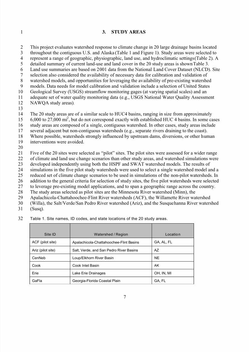
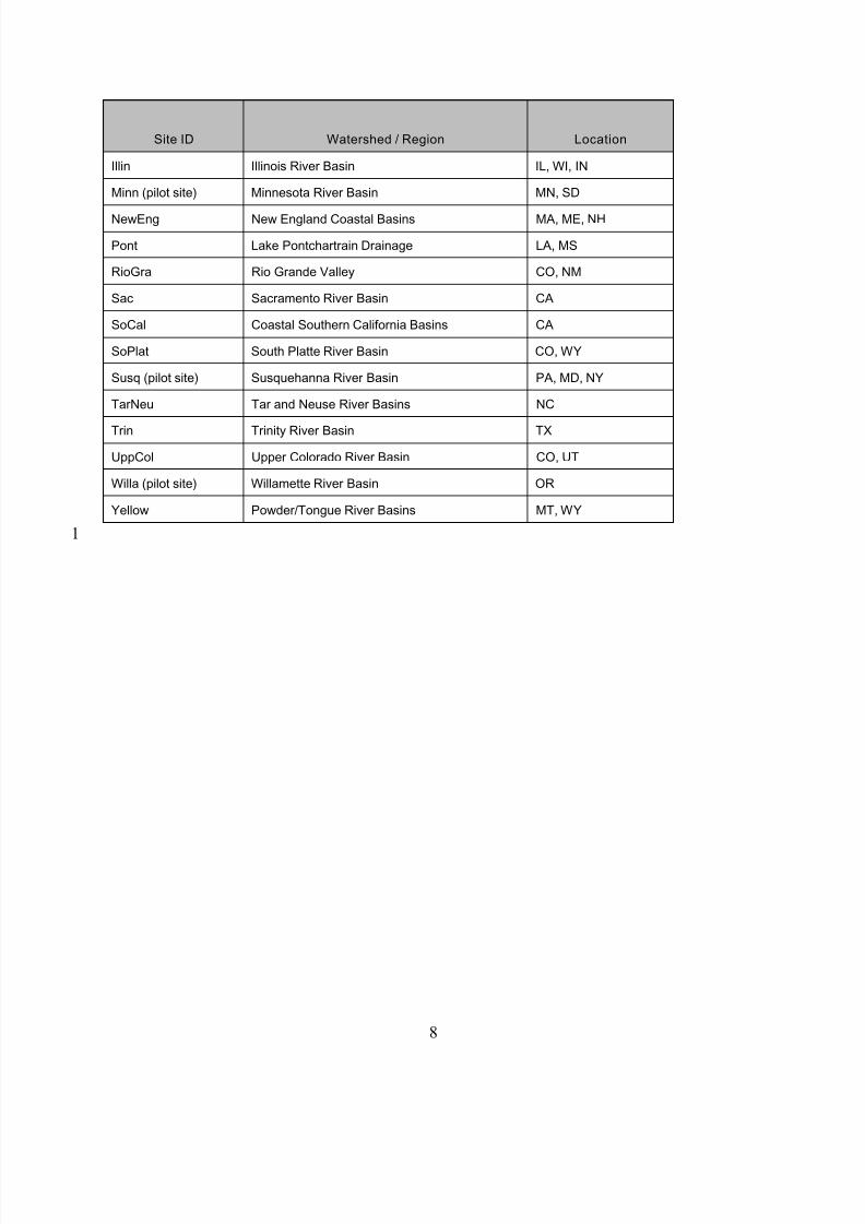
1 3. STUDY AREAS
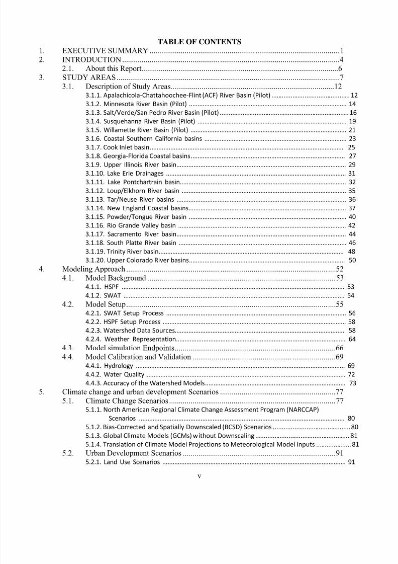
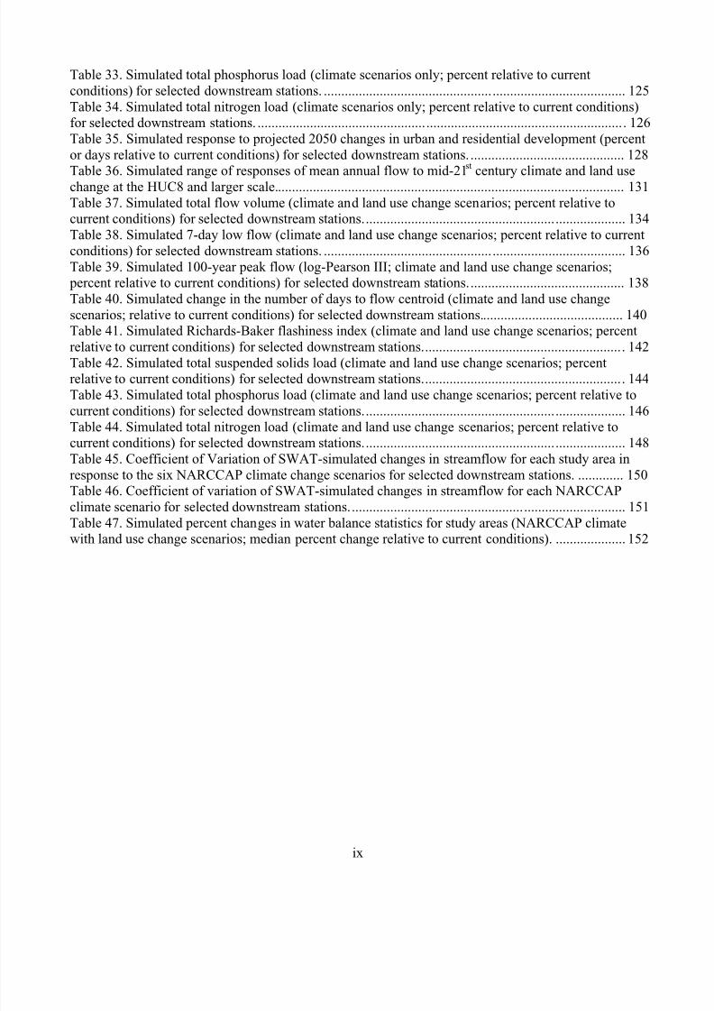
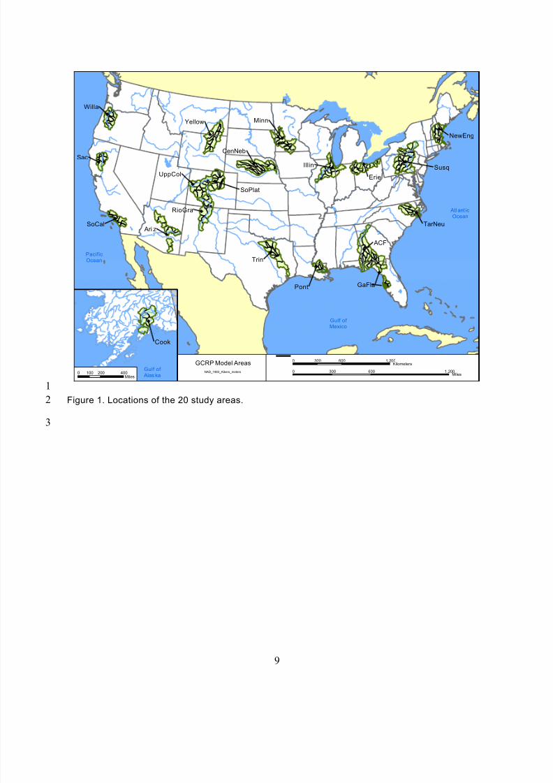
This project evaluates watershed response to climate change in 20 large drainage basins located
throughout the contiguous U.S. and Alaska (Table 1 and Figure 1). Study areas were selected torepresent a range of geographic, physiographic, land use, and hydroclimatic settings (Table 2). A
detailed summary of current land-use and land cover in the 20 study areas is shown Table 3.
Land use summaries are based on 2001 data from the National Land Cover Dataset (NLCD). Siteselection also considered the availability of necessary data for calibration and validation of
watershed models, and opportunities for leveraging the availability of pre-existing watershed
models. Data needs for model calibration and validation include a selection of United StatesGeological Survey (USGS) streamflow monitoring gages (at varying spatial scales) and an
adequate set of water quality monitoring data (e.g., USGS National Water Quality Assessment
NAWQA study areas).
The 20 study areas are of a similar scale to HUC4 basins, ranging in size from approximately
6,000 to 27,000 mi2, but do not correspond exactly with established HUC 4 basins. In some cases
study areas are composed of a single, contiguous watershed. In other cases, study areas includeseveral adjacent but non-contiguous watersheds (e.g., separate rivers draining to the coast).
Where possible, watersheds strongly influenced by upstream dams, diversions, or other human
interventions were avoided.
Five of the 20 sites were selected as “pilot” sites. The pilot sites were assessed for a wider range
of climate and land use change scenarios than other study areas, and watershed simulations weredeveloped independently using both the HSPF and SWAT watershed models. The results of
simulations in the five pilot study watersheds were used to select a single watershed model and a
reduced set of climate change scenarios to be used in simulations of the non-pilot watersheds. In
addition to the general criteria for selection of study sites, the five pilot watersheds were selected
to leverage pre-existing model applications, and to span a geographic range across the country.The study areas selected as pilot sites are the Minnesota River watershed (Minn), the
Apalachicola-Chattahoochee-Flint River watersheds (ACF), the Willamette River watershed(Willa), the Salt/Verde/San Pedro River watershed (Ariz), and the Susquehanna River watershed
(Susq).
Table 1. Site names, ID codes, and state locations of the 20 study areas.
2
34
5
67
8
910
11
12
1314
15
1617
18
1920
21
2223
24
25
26
2728
2930
31
32
7
Site ID Watershed / Region Location
ACF (pilot site) Apalachicola-Chattahoochee-Flint Basins GA, AL, FL
Ariz (pilot site) Salt, Verde, and San Pedro River Basins AZ
CenNeb Loup/Elkhorn River Basin NE
Cook Cook Inlet Basin AK
Erie Lake Erie Drainages OH, IN, MI
GaFla Georgia-Florida Coastal Plain GA, FL
8/13/2019 20 Watersheds Erd
http://slidepdf.com/reader/full/20-watersheds-erd 20/186
Site ID Watershed / Region Location
Illin Illinois River Basin IL, WI, IN
Minn (pilot site) Minnesota River Basin MN, SD
NewEng New England Coastal Basins MA, ME, NH
Pont Lake Pontchartrain Drainage LA, MS
RioGra Rio Grande Valley CO, NM
Sac Sacramento River Basin CA
SoCal Coastal Southern California Basins CA
SoPlat South Platte River Basin CO, W Y
Susq (pilot site) Susquehanna River Basin PA, MD, NY
TarNeu Tar and Neuse River Basins NC
Trin Trinity River Basin TX
UppCol Upper Colorado River Basin CO, UT
Willa (pilot site) Willamette River Basin OR
Yellow Powder/Tongue River Basins MT, W Y
1
8
8/13/2019 20 Watersheds Erd
http://slidepdf.com/reader/full/20-watersheds-erd 21/186
GCRP Model AreasNAD_1983_Albers_meters 0 600 1,200300
Miles ¯
Ari z
Sac
Willa
TarNeu
GaFla
Susq
Pont
UppCol
Trin
ACF
NewEng
MinnYellow
Erie
Illin
SoCal
SoPlat
CenNeb
Atl ant ic
Ocean
Pacific
Ocean
Cook
0 200 400100Miles
Gulf of
Mexico
Gulf of
Alas ka
0 600 1,200300Kilometers
RioGra
9
Figure 1. Locations of the 20 study areas.
1
2
3
8/13/2019 20 Watersheds Erd
http://slidepdf.com/reader/full/20-watersheds-erd 22/186
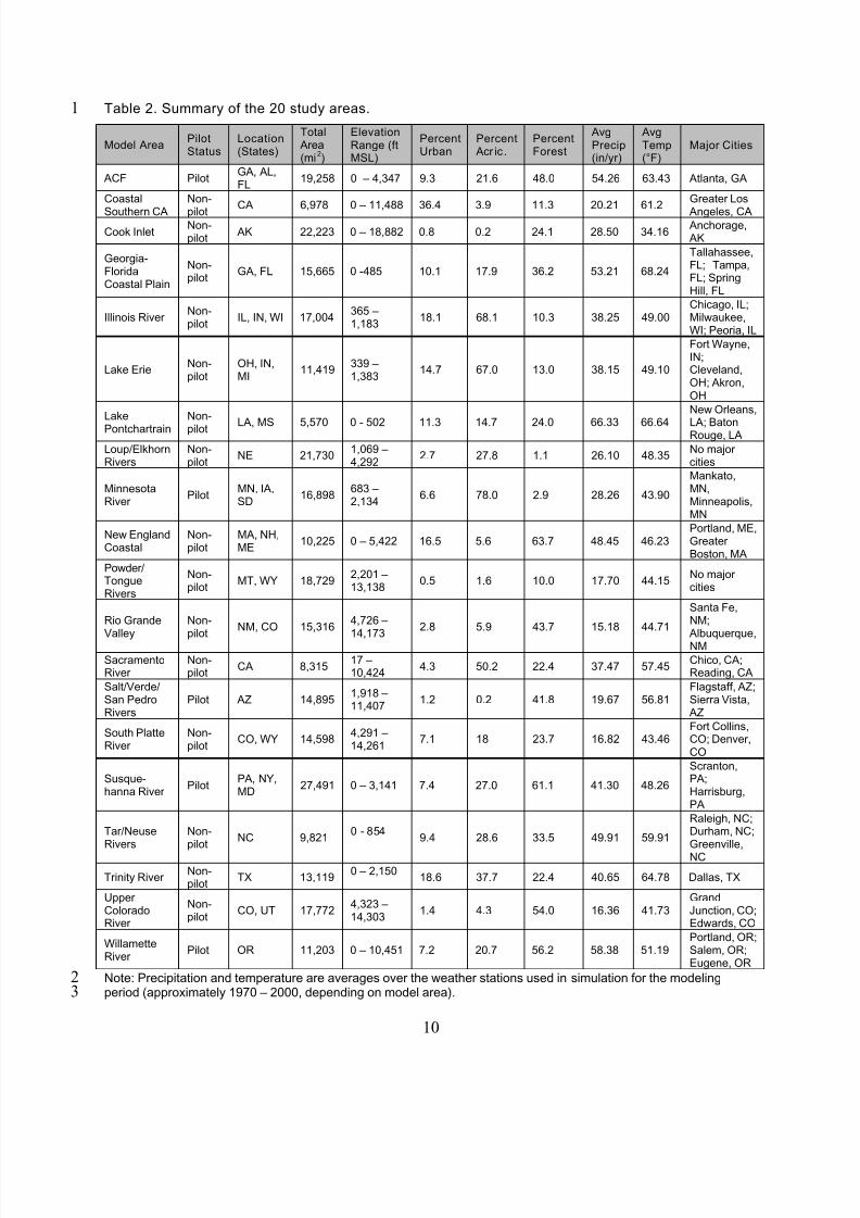
1 Table 2. Summary of the 20 study areas.
23
Model Area
ACF
PilotStatus
Pilot
Location(States)
GA, AL,FL
Total Area(mi
2)
19,258
ElevationRange (ft MSL)
0 – 4,347
PercentUrban
9.3
Percent Acr ic .
21.6
PercentForest
48.0
AvgPrecip(in/yr)
54.26
AvgTemp (°F)
63.43
Major Cities
Atlanta, GA
Coastal
Southern CA
Non-
pilotCA 6,978 0 – 11,488 36.4 3.9 11.3 20.21 61.2
Greater Los
Angeles, CA
Cook InletNon- pilot
AK 22,223 0 – 18,882 0.8 0.2 24.1 28.50 34.16 Anchorage, AK
Georgia-FloridaCoastal Plain
Non- pilotGA, FL 15,665 0 -485 10.1 17.9 36.2 53.21 68.24
Tallahassee,FL; Tampa,FL; SpringHill, FL
Illinois RiverNon- pilot
IL, IN, WI 17,004365 –1,183
18.1 68.1 10.3 38.25 49.00Chicago, IL;Milwaukee,WI; Peoria, IL
Lake ErieNon- pilot
OH, IN,MI
11,419339 –1,383
14.7 67.0 13.0 38.15 49.10
Fort Wayne,IN;Cleveland,OH; Akron,OH
Lake
Pontchartrain
Non-
pilot LA, MS 5,570 0 - 502 11.3 14.7 24.0 66.33 66.64
New Orleans,
LA; BatonRouge, LA
Loup/ElkhornRivers
Non- pilotNE 21,730
1, 069 –4,292
2.7 27.8 1.1 26.10 48.35No majorcities
MinnesotaRiver
PilotMN, IA,SD
16,898683 –2,134
6.6 78.0 2.9 28.26 43.90
Mankato,MN,Minneapolis,MN
New EnglandCoastal
Non- pilotMA, NH,ME
10,225 0 – 5,422 16.5 5.6 63.7 48.45 46.23Portland, ME,GreaterBoston, MA
Powder/TongueRivers
Non- pilotMT, WY 18,729
2, 201 –13,138
0.5 1.6 10.0 17.70 44.15No majorcities
Rio GrandeValley
Non- pilotNM, CO 15,316
4, 726 –14,173
2.8 5.9 43.7 15.18 44.71
Santa Fe,NM;
Albuquerque,NM
SacramentoRiver
Non- pilotCA 8,315
17 –10,424
4.3 50.2 22.4 37.47 57.45Chico, CA;Reading, CA
Salt/Verde/San PedroRivers
Pilot AZ 14,8951, 918 –11,407
1.2 0.2 41.8 19.67 56.81Flagstaff, AZ;Sierra Vista,
AZ
South PlatteRiver
Non- pilotCO, WY 14,598
4, 291 –14,261
7.1 18 23.7 16.82 43.46Fort Collins,CO; Denver,CO
Susquehanna River
PilotPA, NY,MD
27,491 0 – 3,141 7.4 27.0 61.1 41.30 48.26
Scranton,PA;Harrisburg,PA
Tar/NeuseRivers
Non- pilotNC 9,821
0 - 8549.4 28.6 33.5 49.91 59.91
Raleigh, NC;Durham, NC;Greenville,
NC
Trinity RiverNon- pilot
TX 13,1190 – 2,150
18.6 37.7 22.4 40.65 64.78 Dallas, TX
UpperColoradoRiver
Non- pilotCO, UT 17,772
4, 323 –14,303
1.4 4.3 54.0 16.36 41.73GrandJunction, CO;Edwards, CO
WillametteRiver
Pilot OR 11,203 0 – 10,451 7.2 20.7 56.2 58.38 51.19Portland, OR;Salem, OR;Eugene, OR
Note: Precipitation and temperature are averages over the weather stations used in simulation for the modelingperiod (approximately 1970 – 2000, depending on model area).
10
8/13/2019 20 Watersheds Erd
http://slidepdf.com/reader/full/20-watersheds-erd 23/186
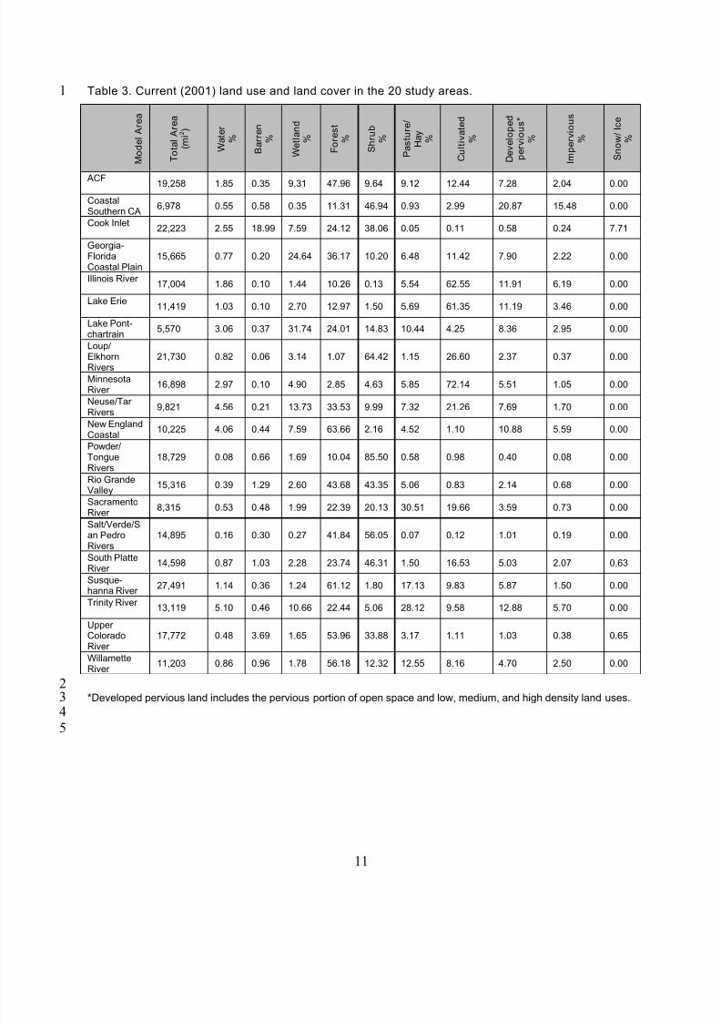
1 Table 3. Current (2001) land use and land cover in the 20 study areas.
M o d e l A r e a
T o t a l A r e a
( m i 2 )
W a t e r
% B a r r e n
%
W e t l a n d
% F o r e s t
% S h r u b
%
P a s t u r e /
H a y
%
C u l t i v a t e d
%
D e v e l o p e d
p e r v i o u s *
%
I m p e r v i o u s
%
S n o w / I c e
%
ACF 19,258 1.85 0.35 9.31 47.96 9.64 9.12 12.44 7.28 2.04 0.00
CoastalSouthern CA
6,978 0.55 0.58 0.35 11.31 46.94 0.93 2.99 20.87 15.48 0.00
Cook Inlet22,223 2.55 18.99 7.59 24.12 38.06 0.05 0.11 0.58 0.24 7.71
Georgia-FloridaCoastal Plain
15,665 0.77 0.20 24.64 36.17 10.20 6.48 11.42 7.90 2.22 0.00
Illinois River17,004 1.86 0.10 1.44 10.26 0.13 5.54 62.55 11.91 6.19 0.00
Lake Erie11,419 1.03 0.10 2.70 12.97 1.50 5.69 61.35 11.19 3.46 0.00
Lake Pontchartrain
5,570 3.06 0.37 31.74 24.01 14.83 10.44 4.25 8.36 2.95 0.00
Loup/
ElkhornRivers
21,730 0.82 0.06 3.14 1.07 64.42 1.15 26.60 2.37 0.37 0.00
MinnesotaRiver
16,898 2.97 0.10 4.90 2.85 4.63 5.85 72.14 5.51 1.05 0.00
Neuse/TarRivers
9,821 4.56 0.21 13.73 33.53 9.99 7.32 21.26 7.69 1.70 0.00
New EnglandCoastal
10,225 4.06 0.44 7.59 63.66 2.16 4.52 1.10 10.88 5.59 0.00
Powder/TongueRivers
18,729 0.08 0.66 1.69 10.04 85.50 0.58 0.98 0.40 0.08 0.00
Rio GrandeValley
15,316 0.39 1.29 2.60 43.68 43.35 5.06 0.83 2.14 0.68 0.00
SacramentoRiver
8,315 0.53 0.48 1.99 22.39 20.13 30.51 19.66 3.59 0.73 0.00
Salt/Verde/S
an PedroRivers
14,895 0.16 0.30 0.27 41.84 56.05 0.07 0.12 1.01 0.19 0.00
South PlatteRiver
14,598 0.87 1.03 2.28 23.74 46.31 1.50 16.53 5.03 2.07 0.63
Susquehanna River
27,491 1.14 0.36 1.24 61.12 1.80 17.13 9.83 5.87 1.50 0.00
Trinity River13,119 5.10 0.46 10.66 22.44 5.06 28.12 9.58 12.88 5.70 0.00
UpperColoradoRiver
17,772 0.48 3.69 1.65 53.96 33.88 3.17 1.11 1.03 0.38 0.65
WillametteRiver
11,203 0.86 0.96 1.78 56.18 12.32 12.55 8.16 4.70 2.50 0.00
23
45
*Developed pervious land includes the pervious portion of open space and low, medium, and high density land uses.
11
8/13/2019 20 Watersheds Erd
http://slidepdf.com/reader/full/20-watersheds-erd 24/186
1
2
3
4
56
7
89
10
1112
13
1415
16
17
1819
20
2122
23
2425
26
27
2829
30
3132
3.1. DESCRIPTION OF STUDY AREAS
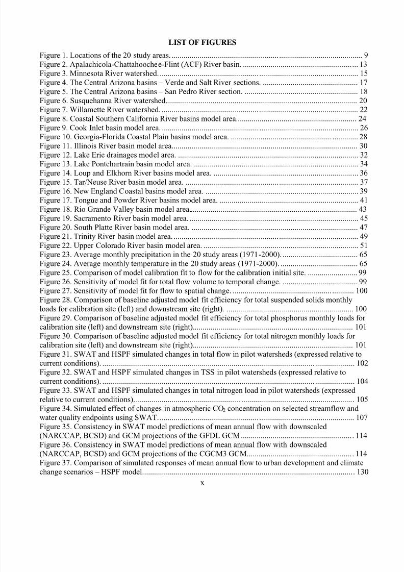
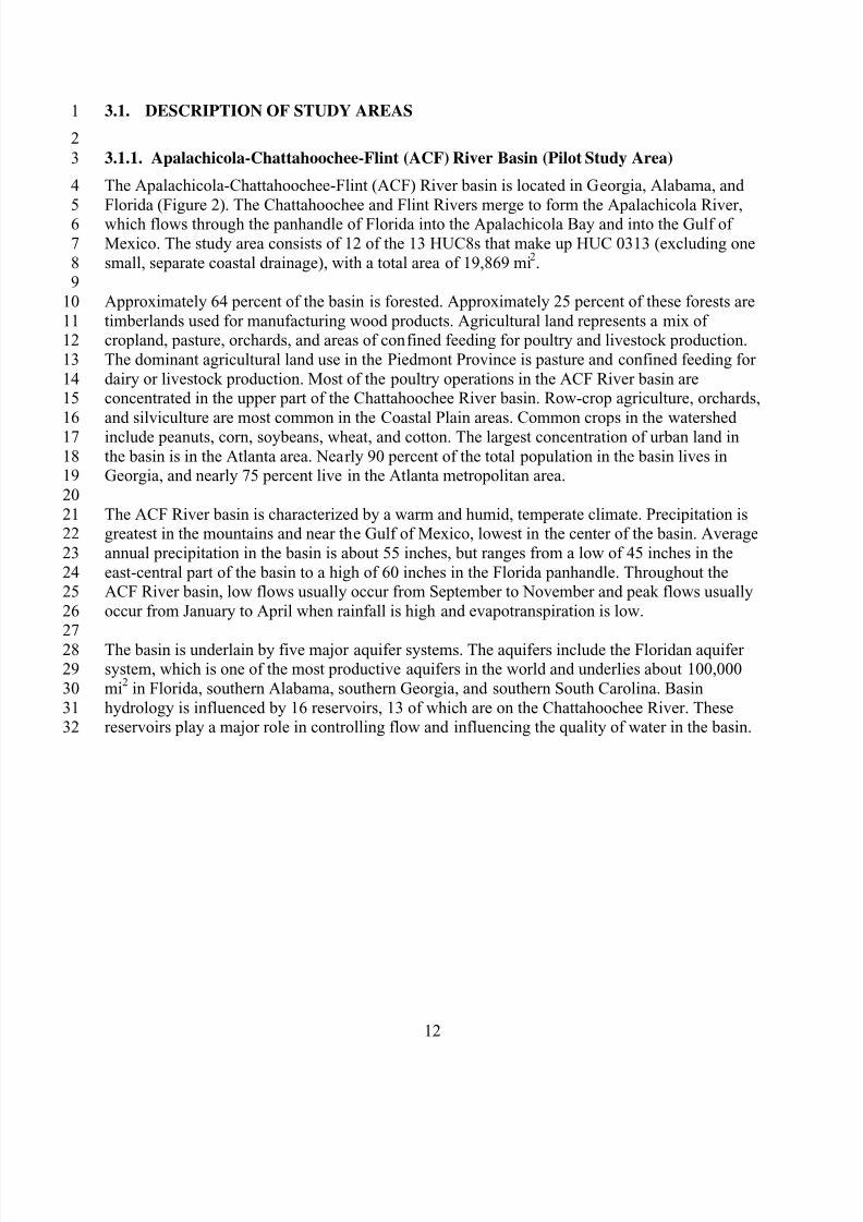
3.1.1. Apalachicola-Chattahoochee-Flint (ACF) River Basin (Pilot Study Area)
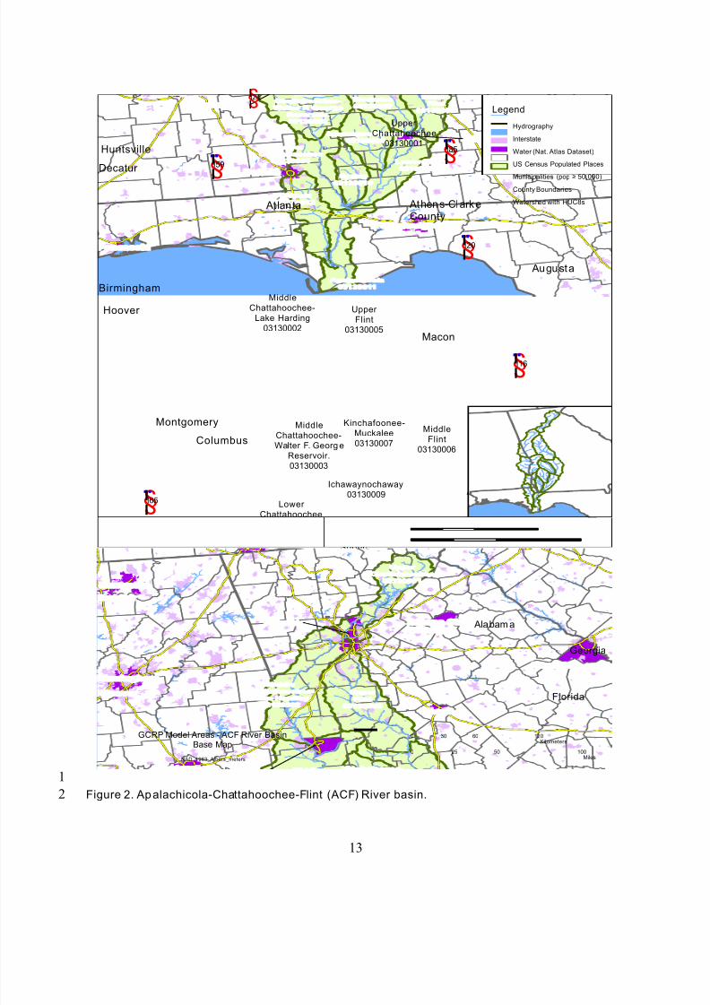
The Apalachicola-Chattahoochee-Flint (ACF) River basin is located in Georgia, Alabama, and
Florida (Figure 2). The Chattahoochee and Flint Rivers merge to form the Apalachicola River,which flows through the panhandle of Florida into the Apalachicola Bay and into the Gulf of
Mexico. The study area consists of 12 of the 13 HUC8s that make up HUC 0313 (excluding one
small, separate coastal drainage), with a total area of 19,869 mi2.
Approximately 64 percent of the basin is forested. Approximately 25 percent of these forests are
timberlands used for manufacturing wood products. Agricultural land represents a mix ofcropland, pasture, orchards, and areas of confined feeding for poultry and livestock production.
The dominant agricultural land use in the Piedmont Province is pasture and confined feeding for
dairy or livestock production. Most of the poultry operations in the ACF River basin areconcentrated in the upper part of the Chattahoochee River basin. Row-crop agriculture, orchards,
and silviculture are most common in the Coastal Plain areas. Common crops in the watershed
include peanuts, corn, soybeans, wheat, and cotton. The largest concentration of urban land in
the basin is in the Atlanta area. Nearly 90 percent of the total population in the basin lives inGeorgia, and nearly 75 percent live in the Atlanta metropolitan area.
The ACF River basin is characterized by a warm and humid, temperate climate. Precipitation isgreatest in the mountains and near the Gulf of Mexico, lowest in the center of the basin. Average
annual precipitation in the basin is about 55 inches, but ranges from a low of 45 inches in the
east-central part of the basin to a high of 60 inches in the Florida panhandle. Throughout theACF River basin, low flows usually occur from September to November and peak flows usually
occur from January to April when rainfall is high and evapotranspiration is low.
The basin is underlain by five major aquifer systems. The aquifers include the Floridan aquifersystem, which is one of the most productive aquifers in the world and underlies about 100,000
mi2 in Florida, southern Alabama, southern Georgia, and southern South Carolina. Basin
hydrology is influenced by 16 reservoirs, 13 of which are on the Chattahoochee River. Thesereservoirs play a major role in controlling flow and influencing the quality of water in the basin.
12
8/13/2019 20 Watersheds Erd
http://slidepdf.com/reader/full/20-watersheds-erd 25/186
1
2
13
At lanta
Columbus
Alabam a
Georgia
Florida
Augusta
§̈¦I20
§̈¦I10
§̈¦I16
§̈¦I65
§̈¦I85
§̈¦I59
§̈¦I385
§̈¦I26
§¦I24
Upper
Flint
03130005
Middle
Flint
03130006
Lower Flint03130008
Middle
Chattahoochee-
Lake Harding
03130002
Middle
Chattahoochee-
Walter F. Georg e
Reservoir.
03130003
Apalachi co la03130011
Upper
Chattahoochee
03130001
Chipola
03130012
Spring
03130010
Ichawaynochaway
03130009
Kinchafoonee-
Muckalee
03130007
Lower
Chattahoochee
03130004
Huntsville
Montgomery
Birmingham
Dothan
Tallahassee
Macon
Albany
Athens-ClarkeCounty
Hoover
Pensacola
Decatur
GCRP Model Areas - ACF River BasinBase Map
NAD_1983_Albers_meters
0 60 12030Kilometers
0 5025Miles
Legend
Hydrography
Interstate
Water (Nat. Atlas Dataset)
US Census Populated Places
Municipalities (pop ≥ 50,000)
County Boundaries
Watershed with HUC8s
Georgia
Alabama
Florida
¯ 100
Figure 2. Apalachicola-Chattahoochee-Flint (ACF) River basin.
8/13/2019 20 Watersheds Erd
http://slidepdf.com/reader/full/20-watersheds-erd 26/186
1
2
3
45
678
9
1011
12
13
1415
16
1718
19
2021
22
23
2425
26
27
2829
30
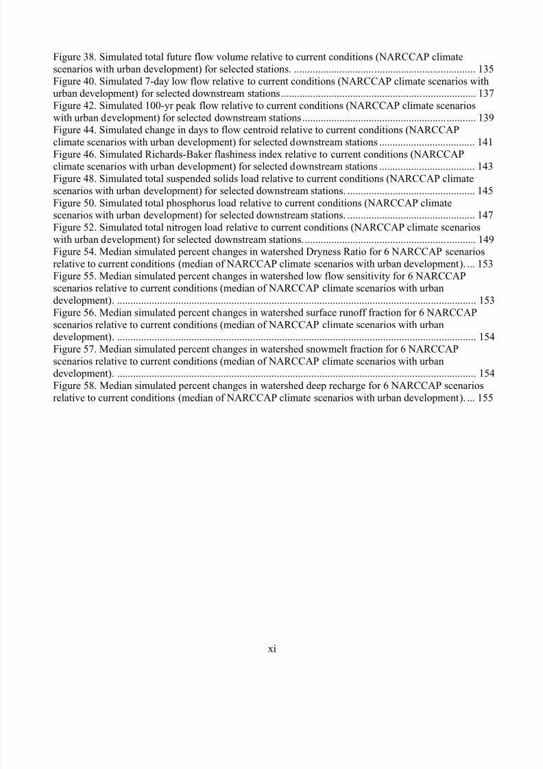
3.1.2. Minnesota River Basin (Pilot Study Area)
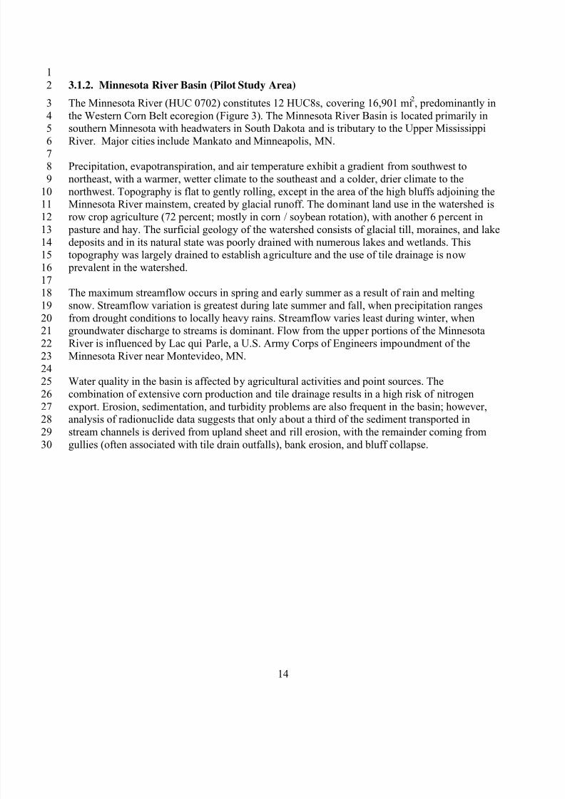
The Minnesota River (HUC 0702) constitutes 12 HUC8s, covering 16,901 mi2, predominantly in
the Western Corn Belt ecoregion (Figure 3). The Minnesota River Basin is located primarily insouthern Minnesota with headwaters in South Dakota and is tributary to the Upper Mississippi
River. Major cities include Mankato and Minneapolis, MN.
Precipitation, evapotranspiration, and air temperature exhibit a gradient from southwest to
northeast, with a warmer, wetter climate to the southeast and a colder, drier climate to the
northwest. Topography is flat to gently rolling, except in the area of the high bluffs adjoining theMinnesota River mainstem, created by glacial runoff. The dominant land use in the watershed is
row crop agriculture (72 percent; mostly in corn / soybean rotation), with another 6 percent in
pasture and hay. The surficial geology of the watershed consists of glacial till, moraines, and lake
deposits and in its natural state was poorly drained with numerous lakes and wetlands. Thistopography was largely drained to establish agriculture and the use of tile drainage is now
prevalent in the watershed.
The maximum streamflow occurs in spring and early summer as a result of rain and melting
snow. Streamflow variation is greatest during late summer and fall, when precipitation ranges
from drought conditions to locally heavy rains. Streamflow varies least during winter, whengroundwater discharge to streams is dominant. Flow from the upper portions of the Minnesota
River is influenced by Lac qui Parle, a U.S. Army Corps of Engineers impoundment of the
Minnesota River near Montevideo, MN.
Water quality in the basin is affected by agricultural activities and point sources. The
combination of extensive corn production and tile drainage results in a high risk of nitrogen
export. Erosion, sedimentation, and turbidity problems are also frequent in the basin; however,
analysis of radionuclide data suggests that only about a third of the sediment transported instream channels is derived from upland sheet and rill erosion, with the remainder coming from
gullies (often associated with tile drain outfalls), bank erosion, and bluff collapse.
14
8/13/2019 20 Watersheds Erd
http://slidepdf.com/reader/full/20-watersheds-erd 27/186
1
2
15
§̈¦I29
§̈¦I35
§̈¦I90
§̈¦I94
Iowa
South Dakota
North Dakota
Minneapolis
Mankato
Minnesota
Chippewa(07020005)
Lower Minnesota(070200012)
Hawk-Yellow Medicine(07020004)
Blue Earth(07020009)
Cottonwood(07020008)
Watonwan(07020010)
Redwood(07020006)
Le Sueur (07020011)
Middle Minnesota(07020007)
Upper Minnesota(07020001)
Pomme De Terre(07020002)
Lac Qui Parle(07020003)
GCRP Model Areas - Minnesota River BasinBase Map
NAD_1983_Albers_meters
0 30 6015Kilometers
0 3015Miles ¯
Legend
Hydrography
Interstate
Water (Nat. Atlas Dataset)
US Census Populated Places
Municipalities (pop ≥ 50,000)
County Boundaries
Watershed with HUC8s
Iowa
Minnesota
60
Figure 3. Minnesota River watershed.
8/13/2019 20 Watersheds Erd
http://slidepdf.com/reader/full/20-watersheds-erd 28/186
1
2
3
45
678
9
1011
12
13
1415
16
1718
19
2021
22
23
2425
26
27
2829
3031
3.1.3. Salt/Verde/San Pedro River Basin (Pilot Study Area)
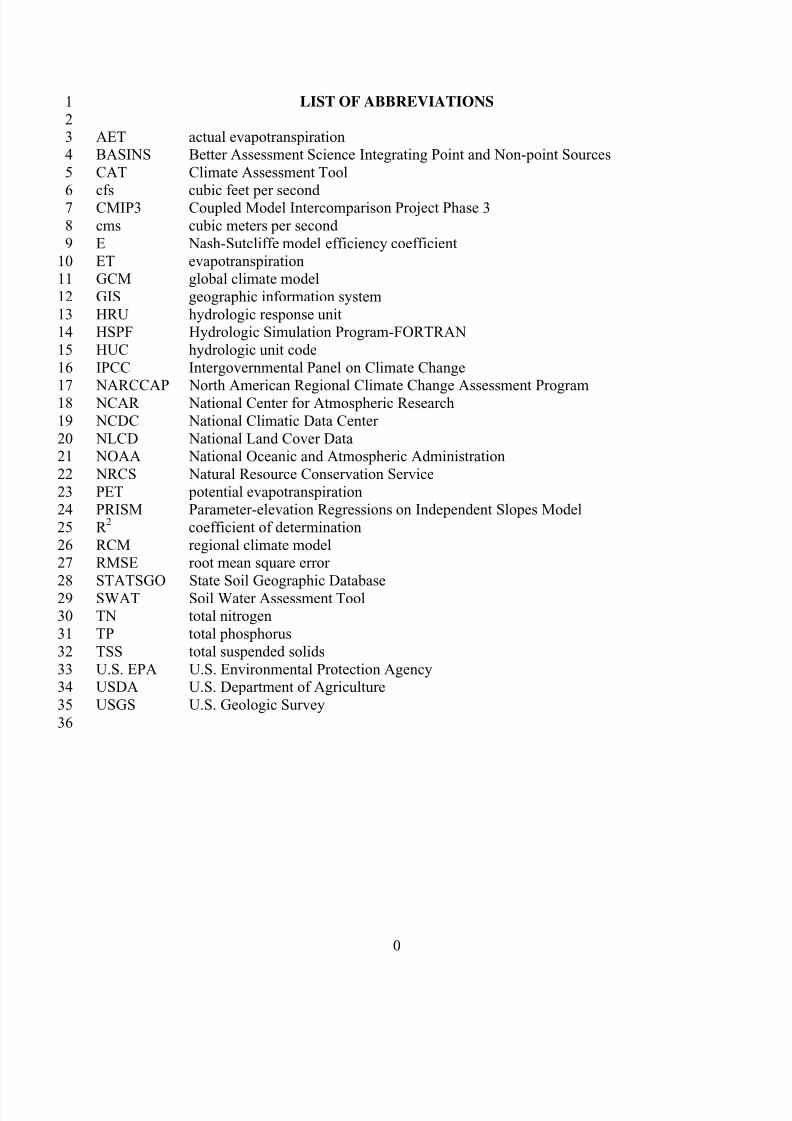
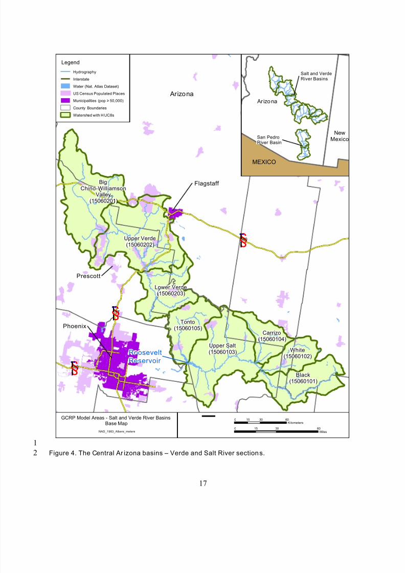
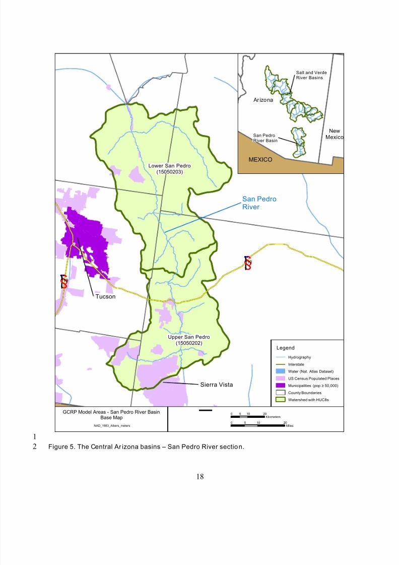
The Central Arizona watersheds include areas dominated by ephemeral streams and significant
impoundments. The selected model area includes perennial portions of the Salt and Verde River
basins (in HUC 1506) that lie upstream of major impoundments, along with the San Pedro River(HUC 1505), for a total of 10 HUC8s with an area of 16,128 mi
2 (Figure 4 and Figure 5).
Land cover is primarily desert scrub and rangeland at low elevations with sparse forest at higherelevations (USGS, 2004; Cordy et al., 2000). The two major population centers of Arizona,
Phoenix and Tucson, are located just downstream of the model area, while portions of Flagstaff,
Prescott, and several smaller towns are within the Verde River watershed. Population growth isresulting in increasing demands on the limited water resources of the area. The climate is arid to
semiarid and is characterized by variability from place to place as well as large differences in
precipitation from one year to the next. Precipitation can be three times greater in wet years than
in dry years.
The Verde and Salt River watersheds are in the Central Highlands hydrologic province,
characterized by mountainous terrain with shallow, narrow intermountain basins. Forests andrangeland cover most of the area with limited areas of agriculture. Perennial streams derive their
flow from mean annual precipitation of more than 25 inches in the mountains. The San Pedro
watershed is in the Basin and Range Lowlands hydrologic province, characterized by deep, broad alluvial basins separated by mountain ranges of small areal extent characterize this
hydrologic province. There is very little natural streamflow because of an average annual rainfall
of less than 10 to 15 inches except at the highest elevations. With the exception of some small,
higher elevation streams and sections of the San Pedro River supported by regional groundwaterdischarge, most perennial streams in the Basin and Range Lowlands are dependent on treated
wastewater effluent for their year-round flow. Rangeland is the predominant land use in the
Basin and Range Lowlands. Because of the general lack of surface water resources in the Basin
and Range Lowlands, groundwater is relied upon heavily to meet agricultural and municipaldemands. More than 50 percent of the water used in the CAZB is groundwater, which is often
the sole source available.
16
8/13/2019 20 Watersheds Erd
http://slidepdf.com/reader/full/20-watersheds-erd 29/186
1
2
17
Roosevelt
Reservoir
Phoenix
Flagstaff
Prescott
Arizona
Upper Verde(15060202)
Upper Salt(15060103)
Black(15060101)
Tonto(15060105)
Lower Verde(15060203)
White(15060102)
Carrizo(15060104)
BigChino-Williamson
Valley
(15060201)
§̈¦I40
§̈¦I17
§̈¦I10
GCRP Model Areas - Salt and Verde River BasinsBase Map
NAD_1983_Albers_meters
0 30 6015Kilometers
0 3015Miles ¯
Legend
Hydrography
Interstate
Water (Nat. Atlas Dataset)
US Census Populated Places
Municipalities (pop ≥ 50,000)
County Boundaries
Watershed with H UC8s
MEXICO
San PedroRiver Basin
Salt and VerdeRiver Basins
Ar izona
NewMexico
60
Figure 4. The Central Ar izona basins – Verde and Salt River sections.
8/13/2019 20 Watersheds Erd
http://slidepdf.com/reader/full/20-watersheds-erd 30/186
1
2
18
Tucson
Sierra Vista
San PedroRiver
Lower San Pedro
(15050203)
Upper San Pedro
(15050202)
§̈¦I10
§̈¦I19
GCRP Model Areas - San Pedro River BasinBase Map
NAD_1983_Albers_meters
0 10 205Kilometers
0 10 205Miles ¯
Legend
Hydrography
Interstate
Water (Nat. Atlas Dataset)
US Census Populated Places
Municipalities (pop ≥ 50,000)
County Boundaries
Watershed with HUC8s
MEXICO
San Pedro
River Basin
Salt and VerdeRiver Basins
Ar izona
NewMexico
Figure 5. The Central Ar izona basins – San Pedro River section.
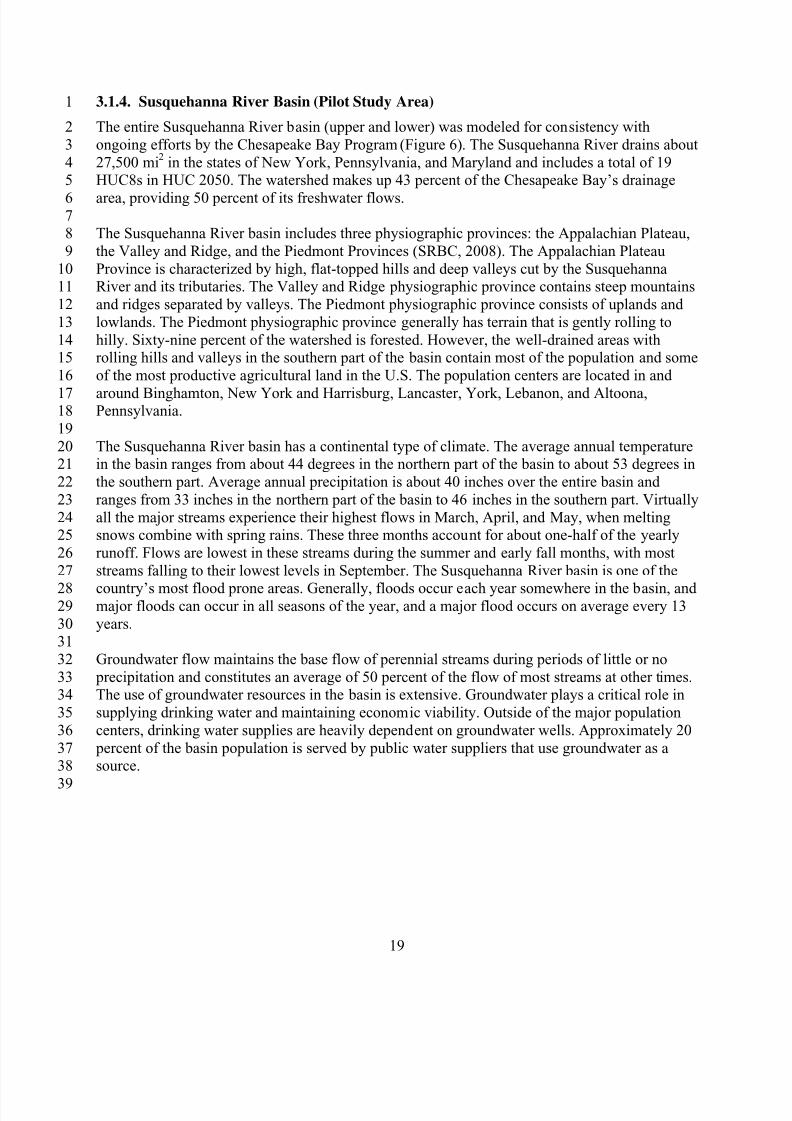
8/13/2019 20 Watersheds Erd
http://slidepdf.com/reader/full/20-watersheds-erd 31/186
1
2
3
45
678
9
1011
12
13
1415
16
1718
19
2021
22
23
2425
26
27
2829
3031
32
3334
35
36
3738
39
3.1.4. Susquehanna River Basin (Pilot Study Area)
The entire Susquehanna River basin (upper and lower) was modeled for consistency with
ongoing efforts by the Chesapeake Bay Program (Figure 6). The Susquehanna River drains about
27,500 mi2
in the states of New York, Pennsylvania, and Maryland and includes a total of 19HUC8s in HUC 2050. The watershed makes up 43 percent of the Chesapeake Bay’s drainage
area, providing 50 percent of its freshwater flows.
The Susquehanna River basin includes three physiographic provinces: the Appalachian Plateau,
the Valley and Ridge, and the Piedmont Provinces (SRBC, 2008). The Appalachian Plateau
Province is characterized by high, flat-topped hills and deep valleys cut by the SusquehannaRiver and its tributaries. The Valley and Ridge physiographic province contains steep mountains
and ridges separated by valleys. The Piedmont physiographic province consists of uplands and
lowlands. The Piedmont physiographic province generally has terrain that is gently rolling to
hilly. Sixty-nine percent of the watershed is forested. However, the well-drained areas withrolling hills and valleys in the southern part of the basin contain most of the population and some
of the most productive agricultural land in the U.S. The population centers are located in and
around Binghamton, New York and Harrisburg, Lancaster, York, Lebanon, and Altoona,Pennsylvania.
The Susquehanna River basin has a continental type of climate. The average annual temperaturein the basin ranges from about 44 degrees in the northern part of the basin to about 53 degrees in
the southern part. Average annual precipitation is about 40 inches over the entire basin and
ranges from 33 inches in the northern part of the basin to 46 inches in the southern part. Virtually
all the major streams experience their highest flows in March, April, and May, when meltingsnows combine with spring rains. These three months account for about one-half of the yearly
runoff. Flows are lowest in these streams during the summer and early fall months, with most
streams falling to their lowest levels in September. The Susquehanna River basin is one of the
country’s most flood prone areas. Generally, floods occur each year somewhere in the basin, andmajor floods can occur in all seasons of the year, and a major flood occurs on average every 13
years.
Groundwater flow maintains the base flow of perennial streams during periods of little or no
precipitation and constitutes an average of 50 percent of the flow of most streams at other times.The use of groundwater resources in the basin is extensive. Groundwater plays a critical role in
supplying drinking water and maintaining economic viability. Outside of the major population
centers, drinking water supplies are heavily dependent on groundwater wells. Approximately 20
percent of the basin population is served by public water suppliers that use groundwater as asource.
19
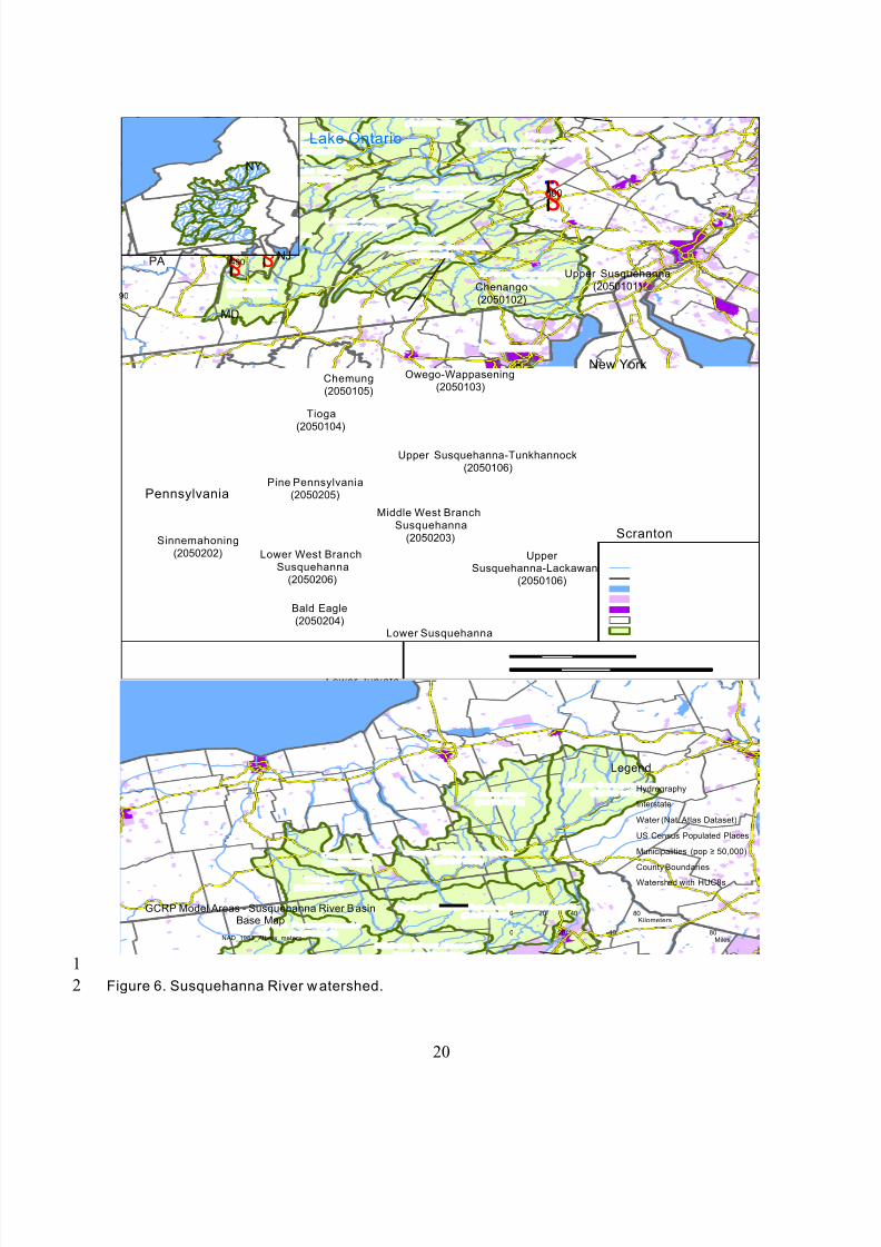
8/13/2019 20 Watersheds Erd
http://slidepdf.com/reader/full/20-watersheds-erd 32/186
1
2
20
Harrisburg
Scranton
Maryland
Pennsylvania
New York
Lake Ontario
BaltimoreWestVirginia
Philadelphia
Pennsylvania
New Jersey
Chenango
(2050102)
Pine Pennsylvania
(2050205)
Lower Susquehanna
(2050306)
Lower Juniata
(2050304)
Upper Susquehanna
(2050101)
Tioga
(2050104)
Lower
Susquehanna-Swatara
(2050305)
Upper Susquehanna-Tunkhannock
(2050106)
Raystown
(2050303)
Lower West Branch
Susquehanna
(2050206)
Upper Susquehanna-Lackawanna
(2050106)
Chemung
(2050105)
Sinnemahoning
(2050202)
Upper Juniata
(2050302)
Lower Susquehanna
(2050301)Upper West B ranch
Susquehanna(2050201)
Bald Eagle
(2050204)
Owego-Wappasening
(2050103)
Middle West Branch
Susquehanna
(2050203)
§̈¦I78
§̈¦I490
§̈¦I90
§̈¦I590
90
GCRP Model Areas - Susquehanna River BasinBase Map
NAD_1983_Albers_meters
0 40 8020Kilometers
0 4020Miles ¯
Legend
Hydrography
Interstate
Water (Nat. Atlas Dataset)
US Census Populated Places
Municipalities (pop ≥ 50,000)
County Boundaries
Watershed with HUC8s
NJ
MDDelaw are
NY
PA
80
Figure 6. Susquehanna River watershed.
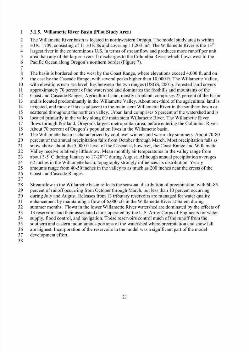
8/13/2019 20 Watersheds Erd
http://slidepdf.com/reader/full/20-watersheds-erd 33/186
1
2
3
45
678
9
1011
12
13
1415
16
1718
19
2021
22
23
2425
26
27
2829
3031
32
3334
35
36
37
38
3.1.5. Willamette River Basin (Pilot Study Area)
The Willamette River basin is located in northwestern Oregon. The model study area is within
HUC 1709, consisting of 11 HUC8s and covering 11,203 mi2. The Willamette River is the 13
th
largest river in the conterminous U.S. in terms of streamflow and produces more runoff per unitarea than any of the larger rivers. It discharges to the Columbia River, which flows west to the
Pacific Ocean along Oregon’s northern border (Figure 7).
The basin is bordered on the west by the Coast Range, where elevations exceed 4,000 ft, and on
the east by the Cascade Range, with several peaks higher than 10,000 ft. The Willamette Valley,
with elevations near sea level, lies between the two ranges (USGS, 2001). Forested land coversapproximately 70 percent of the watershed and dominates the foothills and mountains of the
Coast and Cascade Ranges. Agricultural land, mostly cropland, comprises 22 percent of the basin
and is located predominantly in the Willamette Valley. About one-third of the agricultural land is
irrigated, and most of this is adjacent to the main stem Willamette River in the southern basin orscattered throughout the northern valley. Urban land comprises 6 percent of the watershed and is
located primarily in the valley along the main stem Willamette River. The Willamette River
flows through Portland, Oregon’s largest metropolitan area, before entering the Columbia River.About 70 percent of Oregon’s population lives in the Willamette basin.
The Willamette basin is characterized by cool, wet winters and warm, dry summers. About 70-80
percent of the annual precipitation falls from October through March. Most precipitation falls assnow above about the 5,000 ft level of the Cascades; however, the Coast Range and Willamette
Valley receive relatively little snow. Mean monthly air temperatures in the valley range from
about 3-5oC during January to 17-20
oC during August. Although annual precipitation averages
62 inches in the Willamette basin, topography strongly influences its distribution. Yearlyamounts range from 40-50 inches in the valley to as much as 200 inches near the crests of the
Coast and Cascade Ranges.
Streamflow in the Willamette basin reflects the seasonal distribution of precipitation, with 60-85 percent of runoff occurring from October through March, but less than 10 percent occurring
during July and August. Releases from 13 tributary reservoirs are managed for water qualityenhancement by maintaining a flow of 6,000 cfs in the Willamette River at Salem during
summer months. Flows in the lower Willamette River watershed are dominated by the effects of
13 reservoirs and their associated dams operated by the U.S. Army Corps of Engineers for watersupply, flood control, and navigation. These reservoirs control much of the runoff from the
southern and eastern mountainous portions of the watershed where precipitation and snow fall
are highest. Incorporation of the reservoirs in the model was a significant part of the model
development effort.
21
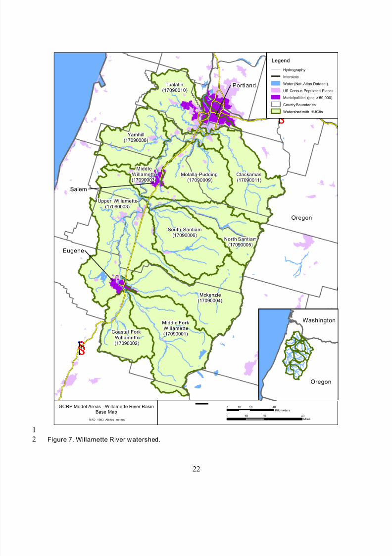
8/13/2019 20 Watersheds Erd
http://slidepdf.com/reader/full/20-watersheds-erd 34/186
1
2
22
Portland
Eugene
Yamhill
(17090008)
Tualatin
(17090010)
Clackamas
(17090011)
Molalla-Pudding
(17090009)
North Santiam
(17090005)
South Santiam
(17090006)
Mckenzie
(17090004)
Middle Fork
Willamette(17090001)Coastal Fork
Willamette
(17090002)
Upper Willamette
(17090003)
Middle
Willamette(17090003)
Salem
Oregon
§̈¦I84
§̈¦I5
GCRP Model Areas - Willamette River BasinBase Map
NAD_1983_Albers_meters
0 20 4010Kilometers
0 20 4010Miles
Legend
Hydrography
Interstate
Water (Nat. Atlas Dataset)
US Census Populated Places
Municipalities (pop ≥ 50,000)
County Boundaries
Watershed with HUC8s
Oregon
Washington
¯ Figure 7. Willamette River watershed.
8/13/2019 20 Watersheds Erd
http://slidepdf.com/reader/full/20-watersheds-erd 35/186
1
2
3
45
678
9
101112
13
1415
16
171819
20
2122
23
24
2526
27
2829
30
3132
33
34
3536
37
38
3940
4142
43
4445
3.1.6. Coastal Southern California basins
The Coastal Southern California basins encompass a land area of over 11,000 mi2 located along the
southern coast of California. The modeled area includes 12 HUC8s within HUC 1807. Major
subbasins included in this study are the Santa Clara River, Los Angeles River, San Gabriel River,Santa Ana River, San Juan River, and Santa Margarita River (Figure 8). The Coastal Southern
California watersheds are characterized by a mild semi-arid climate with an average rainfall of15 inches per year. The region is highly urbanized, with substantial amounts of residential,commercial, and industrial developed land (36 percent) on flatter terrain at lower elevations; the
rugged mountains in the watershed are primarily in forest and rangeland, which together account
for 58 percent of the area.
The Santa Clara River is the largest river system in southern California that remains in a
relatively natural state. The watershed drains 1,634 mi2
from its headwaters in the San Gabriel
Mountains to its mouth at the Pacific Ocean. Ninety percent of the watershed consists of ruggedmountains, ranging up to 8,800 feet high; the reminder consists of valley floor and coastal plain.
The climate in the watershed varies from moist, Mediterranean in Ventura County near the
Pacific coast to near desert at the extreme eastern boundary in Los Angeles County.
The Los Angeles and San Gabriel River watersheds are highly urbanized watersheds that
encompass 835 mi2 and 640 mi
2, respectively. The Los Angeles and San Gabriel Rivers both
originate in mountainous areas including a large portion of the Angeles National Forest. Theyflow from the mountains into the San Fernando and San Gabriel Valleys. The rivers then
continue on over the coastal plain of Los Angeles and eventually into the Pacific Ocean. Both
rivers have been highly modified with dams (51 in the Los Angeles River watershed and 26 in
San Gabriel River watershed). Virtually the entire Los Angeles River has been channelized and paved. The San Gabriel River is also channelized and developed for much of its length. These
modifications have resulted in a loss of habitat and human access to the rivers. Diversion of
water for use in groundwater recharge, significant discharges of sewage treatment plantreclaimed waters, and urban runoff have dramatically changed the natural hydrology of the
rivers.
The Santa Ana River is the largest stream system in southern California and encompasses an area
of about 2,700 mi2
in parts of Orange, San Bernardino, Riverside, and Los Angeles Counties.
The headwaters are in the San Bernardino Mountains, which reach altitudes over 10,000 feet.
The river flows more than 100 miles to the Pacific Ocean. The population of over 4 million people relies on water resources that originate within the watershed as well as water imported
from northern California and the Colorado River. The Santa Ana watershed is highly urbanized
with about 32 percent of the land use residential, commercial, or industrial. Agricultural land use
accounts for about 10 percent of the watershed. Under natural conditions, the Santa Ana Riverwould be intermittent with little or no flow in the summer months. Groundwater is the main
source of water supply in the watershed, providing about 66 percent of the consumptive waterdemand. Imported water from northern California and the Colorado River account for 27 percent
of the consumptive demand. Other sources of supply include surface water derived from
precipitation within the watershed (4 percent) and recycled water (3 percent).
23
8/13/2019 20 Watersheds Erd
http://slidepdf.com/reader/full/20-watersheds-erd 36/186
1
2
34
5
67
8
9
1011
12
13
1415
The San Juan River watershed encompasses about 500 mi2. Watershed concerns include
channelization, poor surface water quality from discharge of nonpoint sources, loss of habitat in
the floodplain, loss of riparian habitat, paving of the flood plain, decline of water supply andflows, biodiversity loss, invasive species, surface erosion, and over use of existing resources. The
majority of the watershed is urbanized.
The Santa Margarita River watershed encompasses 750 mi2. The headwaters are on Palomar
Mountain and there are 27 miles of free-flowing river. It is the least disturbed river system south
of the Santa Ynez River in Santa Barbara County. Unlike most of the rivers of the southern coast
of California, the riparian habitat is of particularly high quality, and is essential for the protectionof waterfowl and a number of endangered plants and animals.
24
Seal Beach
(18070201)
Los Angeles
Palmdale
Lancaster
Riverside
Hesperia
Victorville
Long Beach
San Bernardino
Redlands
Oceanside
Goleta
Hemet
Santa Clarita
Thousand Oaks
Oxnard
Glendale
Temecula
Pasadena
Mission Viejo
Santa Monica
Santa Ana
(18070203)
Santa Clara
(18070102)
Los Angeles
(18070105)
San Jacinto
(18070202)
San Gabriel
(18070106)
Santa Margarita
(18070302)
Santa Monica Bay
(18070104)
Calleguas
(18070103)
Ali so -San On ofr e
(18070301)
Ventura
(18070101)
Newport Bay
(18070204)§̈¦I10
§̈¦I5
§̈¦I15
GCRP Model Areas - Coastal So. Cal. River B asinsBase Map
NAD_1983_Albers_meters
0 20 4010Kilometers
0 20 4010Miles ¯
Legend
Hydrography
Interstate
Water (Nat. Atlas Dataset)
US Census Populated Places
Municipalities (pop ≥ 50,000)
County Boundaries
Watershed with HUC8s
California
Arizon a
Nevada
Figure 8. Coastal Southern Califo rnia River basins model area.
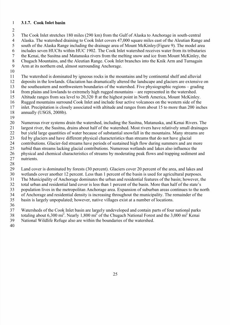
8/13/2019 20 Watersheds Erd
http://slidepdf.com/reader/full/20-watersheds-erd 37/186
1
23
4
56
789
10
11
1213
14
1516
17
1819
20
2122
23
24
2526
27
28
2930
3132
33
34
3536
37
3839
40
3.1.7. Cook Inlet basin
The Cook Inlet stretches 180 miles (290 km) from the Gulf of Alaska to Anchorage in south-central
Alaska. The watershed draining to Cook Inlet covers 47,000 square miles east of the Aleutian Range and
south of the Alaska Range including the drainage area of Mount McKinley (Figure 9). The model areaincludes seven HUC8s within HUC 1902. The Cook Inlet watershed receives water from its tributaries
the Kenai, the Susitna and Matanuska rivers from the melting snow and ice from Mount McKinley, theChugach Mountains, and the Aleutian Range. Cook Inlet branches into the Knik Arm and TurnagainArm at its northern end, almost surrounding Anchorage.
The watershed is dominated by igneous rocks in the mountains and by continental shelf and alluvial
deposits in the lowlands. Glaciation has dramatically altered the landscape and glaciers are extensive onthe southeastern and northwestern boundaries of the watershed. Five physiographic regions – grading
from plains and lowlands to extremely high rugged mountains – are represented in the watershed.
Altitude ranges from sea level to 20,320 ft at the highest point in North America, Mount McKinley.Rugged mountains surround Cook Inlet and include four active volcanoes on the western side of the
inlet. Precipitation is closely associated with altitude and ranges from about 15 to more than 200 inches
annually (USGS, 2008b).
Numerous river systems drain the watershed, including the Susitna, Matanuska, and Kenai Rivers. The
largest river, the Susitna, drains about half of the watershed. Most rivers have relatively small drainages but yield large quantities of water because of substantial snowfall in the mountains. Many streams are
fed by glaciers and have different physical characteristics than streams that do not have glacial
contributions. Glacier-fed streams have periods of sustained high flow during summers and are more
turbid than streams lacking glacial contributions. Numerous wetlands and lakes also influence the physical and chemical characteristics of streams by moderating peak flows and trapping sediment and
nutrients.
Land cover is dominated by forests (30 percent). Glaciers cover 20 percent of the area, and lakes andwetlands cover another 12 percent. Less than 1 percent of the basin is used for agricultural purposes.
The Municipality of Anchorage dominates the urban and residential features of the basin; however, thetotal urban and residential land cover is less than 1 percent of the basin. More than half of the state’s
population lives in the metropolitan Anchorage area. Expansion of suburban areas continues to the north
of Anchorage and residential density is increasing throughout the municipality. The remainder of the
basin is largely unpopulated; however, native villages exist at a number of locations.
Watersheds of the Cook Inlet basin are largely undeveloped and contain parts of four national parks
totaling about 6,300 mi2. Nearly 1,800 mi
2 of the Chugach National Forest and the 3,000 mi
2Kenai
National Wildlife Refuge also are within the boundaries of the watershed.
25
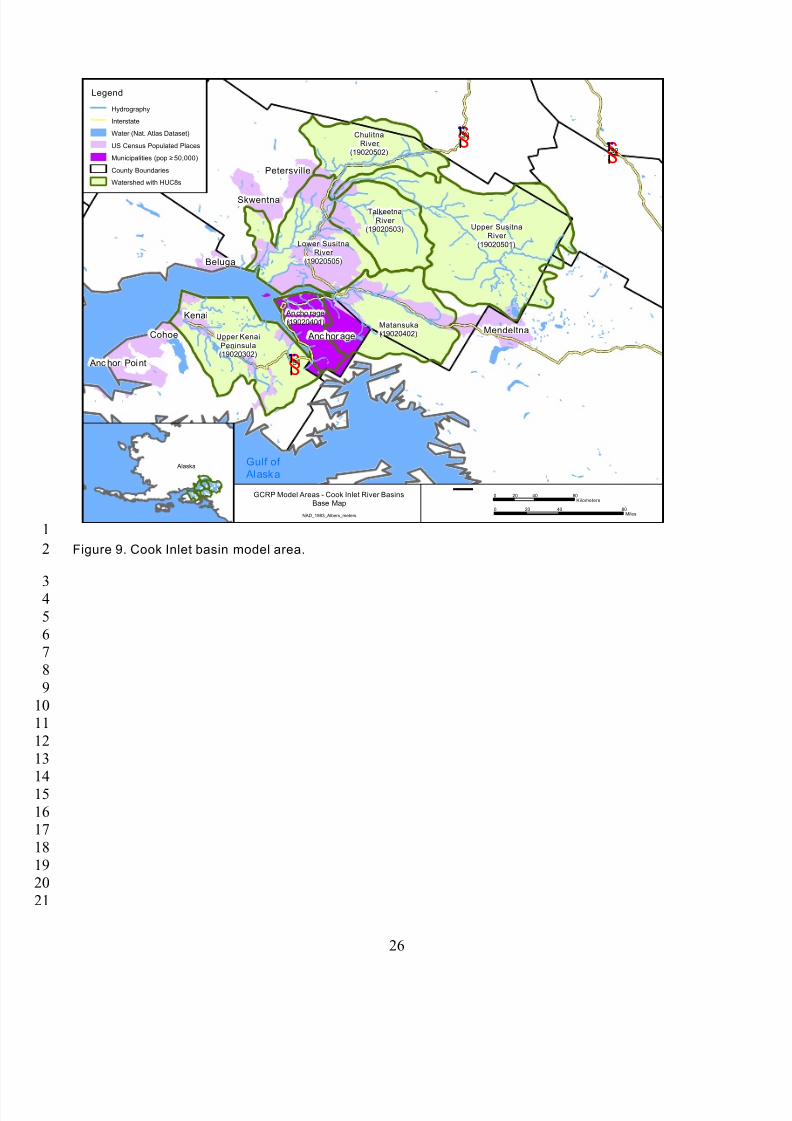
8/13/2019 20 Watersheds Erd
http://slidepdf.com/reader/full/20-watersheds-erd 38/186
1
2
34
5
67
8
9
1011
12
1314
15
1617
18
1920
21
26
Upper Susitna
River
(19020501)
Matansuka
(19020402)
Chulitna
River
(19020502)
Lower Susitna
River
(19020505)
Upper Kenai
Peninsula(19020302)
Talkeetna
River
(19020503)
An cho rage
(19020401)
Anc hor age
Skwentna
Mendeltna
Petersville
Beluga
Cohoe
Anc hor Point
Kenai
Gulf of
Alaska
§̈¦S3
§̈¦S1
§̈¦S2
GCRP Model Areas - Cook Inlet River BasinsBase Map
NAD_1983_Albers_meters
0 40 8020Kilometers
0 4020Miles ¯
Legend
Hydrography
Interstate
Water (Nat. Atlas Dataset)
US Census Populated Places
Municipalities (pop ≥ 50,000)
County Boundaries
Watershed with HUC8s
Alaska
80
Figure 9. Cook Inlet basin model area.
8/13/2019 20 Watersheds Erd
http://slidepdf.com/reader/full/20-watersheds-erd 39/186
1
23
4
56
789
10
11
1213
14
1516
17
1819
20
2122
3.1.8. Georgia-Florida Coastal basins
The Georgia-Florida Coastal Plain basins model covers an area about 15,665 mi2 in portions of Georgia
and Florida. The modeled area includes 15 HUC8s in two groups, one group draining to Tampa Bay
(HUC 0310) and the remainder in southern Georgia and northwest Florida (in HUC 0311 and 0312;
Figure 10). The watershed contains an EPA ORD Ecosystems Research Area (in the Tampa Baydrainage) and Tampa Bay is part of EPA’s National Estuary Program.
Climate in the watershed is humid subtropical and influenced by air masses from the Gulf of Mexico.Average annual rainfall is around 45 to 53 inches per year, while the average annual temperatures is
around 70 – 72 °F. The majority of precipitation is associated with summer convective storms, and
tropical storms cross the area frequently.
The major land uses in the watershed include forest, agriculture (citrus and row crops), wetlands, urban,
and rangeland. Forested areas cover approximately 36 percent of the watershed. Much of the forest lands
are softwood pines used to manufacture paper products (facial tissue, toilet paper, hand towels, bags,and boxes). Wetlands occupy about 25 percent of the watershed. Cultivated land covers approximately
11 percent, while developed land occupies over 10 percent of the area.
The populations of cities in the watershed increased from 10 to 30 percent between 1990 and 1999. The
largest city in the watershed is Tampa, FL. Most water used in the watershed is derived from
groundwater, primarily from the highly productive Floridan aquifer system.
27
8/13/2019 20 Watersheds Erd
http://slidepdf.com/reader/full/20-watersheds-erd 40/186
1
2
3
28
ULF OF MEXICO
Georgia
Florida
Jacksonville
Tampa
Tallahassee
Albany
Spring Hill
Gainesville
St. Petersburg
Clearwater
§̈¦I10
§̈¦I95
§̈¦I75
§̈¦I95
§̈¦I4
Santa Fe(03110206)
Upper Suwannee(03110201)
Alapaha
(03110202)
Lower
Suwannee
(03110205)
Little
(03110204)
Withlacoochee(03110203)
Lower
Ochlockonee(03120003)
Au ci lla(03110103)
Crystal-Pithlachascotee
(03100207)
Upper
Ochlockonee(03120002)
Hillsborough(03100205)
Apalachee Bay -St. Marks
(03120001)
Tampa Bay(03100206)
Alafi a(03100204)
Little Manatee
(03100203)
GCRP Model Areas - Georgia/Florida River BasinsBase Map
NAD_1983_Albers_meters
0 4020Miles
Legend
Hydrography
Interstate
Water (Nat. Atlas Dataset)
US Census Populated Places
Municipalities (pop ≥ 50,000)
County Boundaries
Watershed with HUC8s
GULF OF
MEXICO
Florida
Georgia
0 40 8020Kilometers
80 ¯ Figure 10. Georgia-Florida Coastal Plain basins model area.
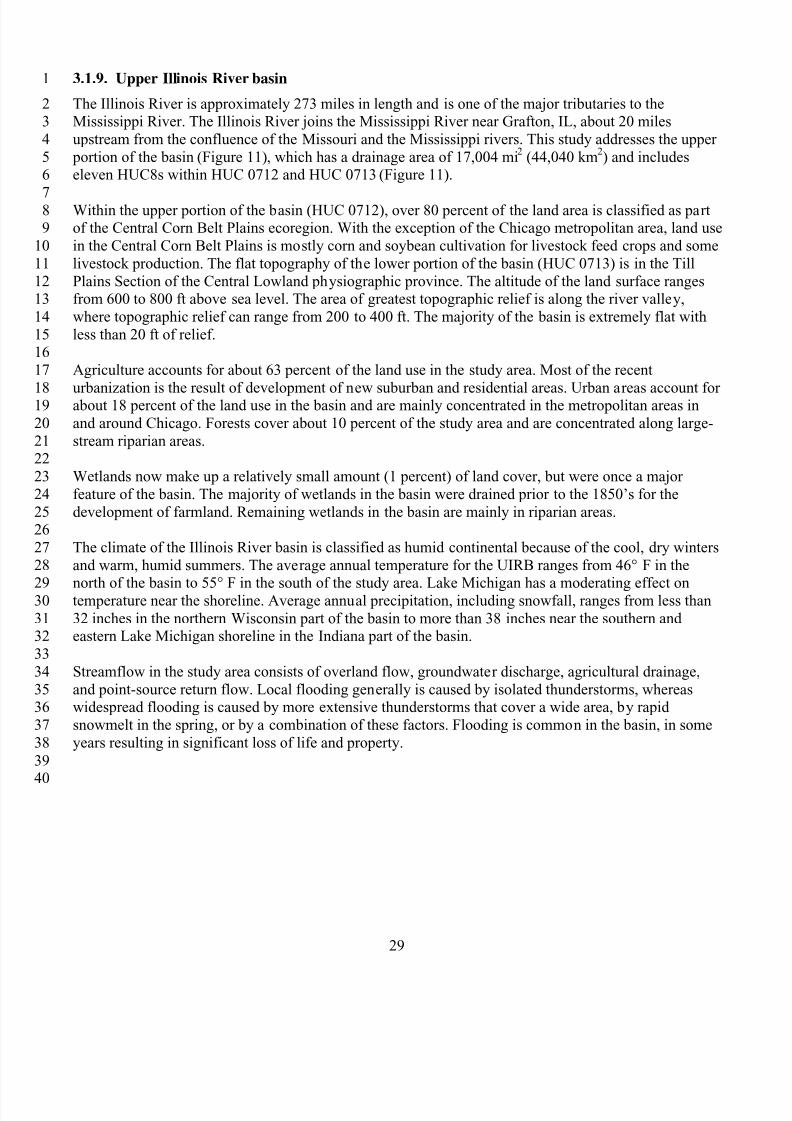
8/13/2019 20 Watersheds Erd
http://slidepdf.com/reader/full/20-watersheds-erd 41/186
1
23
4
56
789
10
11
1213
14
1516
17
1819
20
2122
23
24
2526
27
28
2930
3132
33
34
3536
37
38
39
40
3.1.9. Upper Illinois River basin
The Illinois River is approximately 273 miles in length and is one of the major tributaries to theMississippi River. The Illinois River joins the Mississippi River near Grafton, IL, about 20 miles
upstream from the confluence of the Missouri and the Mississippi rivers. This study addresses the upper
portion of the basin (Figure 11), which has a drainage area of 17,004 mi2 (44,040 km
2) and includes
eleven HUC8s within HUC 0712 and HUC 0713 (Figure 11).
Within the upper portion of the basin (HUC 0712), over 80 percent of the land area is classified as partof the Central Corn Belt Plains ecoregion. With the exception of the Chicago metropolitan area, land use
in the Central Corn Belt Plains is mostly corn and soybean cultivation for livestock feed crops and some
livestock production. The flat topography of the lower portion of the basin (HUC 0713) is in the Till
Plains Section of the Central Lowland physiographic province. The altitude of the land surface rangesfrom 600 to 800 ft above sea level. The area of greatest topographic relief is along the river valley,
where topographic relief can range from 200 to 400 ft. The majority of the basin is extremely flat with
less than 20 ft of relief.
Agriculture accounts for about 63 percent of the land use in the study area. Most of the recent
urbanization is the result of development of new suburban and residential areas. Urban areas account forabout 18 percent of the land use in the basin and are mainly concentrated in the metropolitan areas in
and around Chicago. Forests cover about 10 percent of the study area and are concentrated along large-
stream riparian areas.
Wetlands now make up a relatively small amount (1 percent) of land cover, but were once a major
feature of the basin. The majority of wetlands in the basin were drained prior to the 1850’s for the
development of farmland. Remaining wetlands in the basin are mainly in riparian areas.
The climate of the Illinois River basin is classified as humid continental because of the cool, dry winters
and warm, humid summers. The average annual temperature for the UIRB ranges from 46° F in the
north of the basin to 55° F in the south of the study area. Lake Michigan has a moderating effect ontemperature near the shoreline. Average annual precipitation, including snowfall, ranges from less than
32 inches in the northern Wisconsin part of the basin to more than 38 inches near the southern andeastern Lake Michigan shoreline in the Indiana part of the basin.
Streamflow in the study area consists of overland flow, groundwater discharge, agricultural drainage,
and point-source return flow. Local flooding generally is caused by isolated thunderstorms, whereaswidespread flooding is caused by more extensive thunderstorms that cover a wide area, by rapid
snowmelt in the spring, or by a combination of these factors. Flooding is common in the basin, in some
years resulting in significant loss of life and property.
29
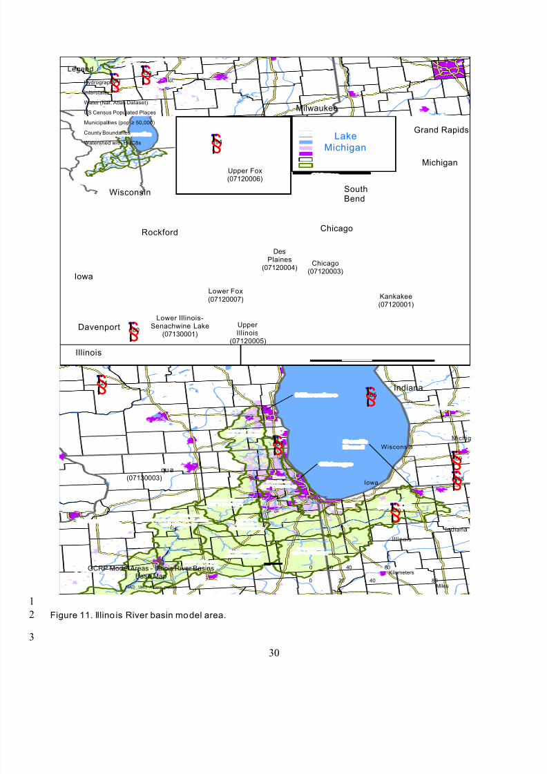
8/13/2019 20 Watersheds Erd
http://slidepdf.com/reader/full/20-watersheds-erd 42/186
1
2
3
30
SouthBend
§̈¦65
Milwaukee
Chicago
Springfield
Davenport
Peoria
Bloomington
Grand Rapids
Lafayette
Rockford
Illinois
Indiana
Iroquois
(07120002)
Kankakee(07120001)
Vermilion(07130002)
Mackinaw
(07130004)
Lower Fox
(07120007)
Upper Fox(07120006)
Lower Illinois-Senachwine Lake
(07130001)
Upper
Illinois(07120005)
DesPlaines
(07120004)
Lower Illinois-Lake Chautauqua
(07130003)
Chicago
(07120003)
Illinois
Indiana
Wisconsin
Michigan
Iowa
LakeMichigan
§̈¦I57
§̈¦I65
§̈¦I74
§̈¦I70
§̈¦I94
§̈¦I39
§̈¦I90
§̈¦I80
§̈¦I69
§̈¦I465
GCRP Model Areas - Illnois River BasinsBase Map
NAD_1983_Albers_meters
0 4020Miles ¯
Legend
Hydrography
Interstate
Water (Nat. Atlas Dataset)
US Census Populated Places
Municipalities (pop ≥ 50,000)
County BoundariesWatershed with HUC8s
Illinois
Indiana
Iowa
Wisconsin
Michig
0 40 8020Kilometers
80
Figure 11. Illino is River basin model area.
8/13/2019 20 Watersheds Erd
http://slidepdf.com/reader/full/20-watersheds-erd 43/186
1
23
4
56
789
10
11
1213
14
1516
17
1819
20
2122
23
24
2526
27
28
2930
3132
33
34
3536
3.1.10. Lake Erie Drainages
Lake Erie is the eleventh largest freshwater lake in the world. About two-thirds of the contributing
watershed is in the United States, and includes portions of Michigan, Indiana, Ohio, Pennsylvania, and
New York. The model study area focuses on drainages to the southwestern portion of Lake Erie andencompasses over 11,400 mi
2 in 11 HUC8s, all within HUC 0411 (Figure 12).
Situated in two major physiographic provinces, the Appalachian Plateaus and the Central Lowland, thewatershed includes varied topographic and geomorphic features that affect the hydrology. The
watershed consists of multiple independent drainages. The principal river in the study unit, the Maumee
River, drains an area of 6,608 mi², or roughly one-third of the model study area. Other principal streams
and their drainage areas in Ohio are the Sandusky River (1,420 mi ², the Cuyahoga River (809 mi ²), andthe Grand River (705 mi²). The land surface is gently rolling to nearly flat (Myers et al., 2000).
The majority of the land use in the model area is agriculture (61 percent). The remaining land uses areurban land (18 percent), forest (10 percent), and open water or wetlands (3 percent). Corn, soybeans, and
wheat are the typical parts in the western part of the basin. Other agricultural land uses include pasture
and forage crops, grown predominantly in the eastern part of the basin. Forest and wetlands have beengreatly reduced in the watershed since the mid-1800s. Major urban areas in the model area include
Cleveland, Toledo, and Akron, Ohio, along with Fort Wayne, Indiana. These cities are important
industrial and manufacturing centers. Major urban centers rely on abundant supplies of water forshipping, electric power generation, industry, domestic consumption, and waste assimilation.
Average annual precipitation across the model study area ranges from about 30 to 45 inches.
Precipitation is highest to the northeast because of lake effect. The lowest amounts of precipitation are inthe northwestern part of the basin near the Michigan border. The highest streamflows are typically in
February, March, and April, as a result of increased precipitation, cold temperatures and little vegetative
growth. The lowest streamflows are in August, September, and October. During low streamflow,
groundwater typically contributes most of the flow.
Cooling during power generation accounts for 71 percent of the water use in the watershed. Public anddomestic supply account for 17 percent, and industry and mining account for 10 percent of the total
water use. Normal precipitation is generally adequate for agriculture, so irrigation accounts for less than
1 percent of water use. Most of the major cities are near Lake Erie and Lake Saint Clair and derive their
water from the lakes or their connecting channels.
31
8/13/2019 20 Watersheds Erd
http://slidepdf.com/reader/full/20-watersheds-erd 44/186
1
2
34
5
6
78
9
10
1112
13
1415
16
1718
19
20
21
32
Lake
Erie
Lake
Erie
Lake
Erie
Lake
Erie
Sandusky(04100011)
Aug laize(04100007)
Grand
(04110004)
Lower Maumee(04100009)
Cuyahoga(04110002)
Black-Rocky(04110001)
Blanchard(04100008)
Tiffin(04100006)
St. Marys(04100004)
Huron-Vermilion
(04100012)
St. Joseph(04100003)
Upper Maumee
(04100005)
Columbus
Detroit
Toledo
Ak ron
Cleveland
Fort Wayne
Canton
Battle Creek
Mentor
Lorain
Muncie
Canton
§̈¦I80
§̈¦I70
§̈¦I75
§̈¦I69
§̈¦I90
Ohio
Michigan
Indiana
GCRP Model Areas - Erie/St. Clair Rive r BasinsBase Map
NAD_1983_Albers_meters
0 30 6015Kilometers
0 3015Miles ¯
Legend
Hydrography
Interstate
Water (Nat. Atlas Dataset)
US Census Populated Places
Municipalities (pop ≥ 50,000)
County Boundaries
Watershed with HUC8s
Michigan
Ohi
Pennsylvani
Ohio
Lake
Erie
60
Figure 12. Lake Erie drainages model area.
3.1.11. Lake Pontchartrain basin
The Acadian-Pontchartrain NAWQA study area encompasses 26,408 mi2 in the southern half of
Louisiana and includes downstream portions of major rivers, such as the Mississippi with drainage areas
far larger than the target size for this project. Therefore, the focus of modeling in this study was thePontchartrain portion of the study area, including the rivers that drain to Lake Pontchartrain and the
cities of New Orleans and Baton Rouge (Figure 13). The resulting model area encompasses over 5,500
mi2 and seven HUC8s within HUCs 0807 and 0809.
The entire model area is near sea level and frequently impacted by tropical storms from the Gulf of
Mexico. The climate is classified as humid subtropical, with an average annual temperature around 70
°F and average annual precipitation of 64 inches per year (USGS, 2002).
Ecosystems and communities in the watershed include cypress-tupelo swamp; freshwater marsh;
saltwater marsh; wet prairie; oak cheniers; bottomland hardwood forest; Piney Hills; and longleaf pinesavanna. The coastal zone of the watershed is affected by the ocean and its tides. Different wetland types
are determined by the salinity of the water in them, which may infiltrate naturally through bayous or
reach further inland through canals.
8/13/2019 20 Watersheds Erd
http://slidepdf.com/reader/full/20-watersheds-erd 45/186
12
3
45
6
7
89
10
1112
13
1415
16
1718
Land uses include a mixture of urban and rapidly urbanizing/industrial areas (11 percent), large areas ofmixed forest and pasture (34 percent), wetlands (32 percent) and areas of rice and sugarcane crops (4
percent). Population is rapidly increasing on the north shore of Lake Pontchartrain and surrounding
Baton Rouge, causing changes in rainfall-runoff characteristics and quality. Urban streams in the BatonRouge area are usually channelized, and cleared of woody vegetation to speed drainage during high
water.
Surface water in the watershed includes the lower Mississippi delta and wet prairie streams as well asupland streams. Lower Mississippi delta and wet prairie streams tend to have very slow flow, and water
can also be pushed upstream by tides or wind causing generally stagnant, backwater conditions.
Wetlands develop naturally in poorly drained areas. Streams in the uplands have a moderate flowgradient and sandy, shifting beds that are reshaped quickly in the fast water that is usual for flood
conditions.
Modifications to flow include levees, and canals and drainage. Levees are created both naturally during
the flooding process (sediment drops out of floodwater next to the waterbody) and by man along many
bayous and rivers to reduce floods and to maintain a deeper channel for shipping.
33
8/13/2019 20 Watersheds Erd
http://slidepdf.com/reader/full/20-watersheds-erd 46/186
1
34
2
Louisiana
Mississippi
Lake Maurepas(08070204)
Am ite(08070202)
Tickpaw(08070203)
Tangipahoa(08070205)
Liberty Bayou-Tchefuncta(08090201)
Bayou Sara-
Thompson(08070201)
Eastern L ouisianaCoastal
(08090203)§̈¦I10
§̈¦I59
§̈¦I55
New Orleans
Baton Rouge
GCRP Model Areas - Pontchartrain BasinBase Map
NAD_1983_Albers_meters
0 2010Miles ¯
Legend
Hydrography
Interstate
Water (Nat. Atlas Dataset)
US Census Populated Places
Municipalities (pop ≥ 50,000)
County BoundariesWatershed with HUC8s
Arkansas
Louisiana Mississippi
0 20 4010Kilometers
Lake
Pontchartrain
40
Figure 13. Lake Pontchartrain basin model area.
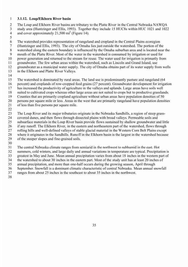
8/13/2019 20 Watersheds Erd
http://slidepdf.com/reader/full/20-watersheds-erd 47/186
1
23
4
56
789
10
11
1213
14
1516
17
1819
20
2122
23
24
2526
27
28
2930
3132
33
34
3536
37
38
3.1.12. Loup/Elkhorn River basin
The Loup and Elkhorn River basins are tributary to the Platte River in the Central Nebraska NAWQAstudy area (Huntzinger and Ellis, 1993). Together they include 15 HUC8s within HUC 1021 and 1022
and cover approximately 21,500 mi2 (Figure 14).
The watershed provides representation of rangeland and cropland in the Central Plains ecoregion
(Huntzinger and Ellis, 1993). The city of Omaha lies just outside the watershed. The portion of thewatershed along the eastern boundary is influenced by the Omaha suburban area and is located near themouth of the Platte River. Most of the water in the watershed is consumed by irrigation or used for
power generation and returned to the stream for reuse. The water used for irrigation is primarily from
groundwater. The few urban areas within the watershed, such as Lincoln and Grand Island, use
groundwater as a municipal water supply. The city of Omaha obtains part of its water supply from wellsin the Elkhorn and Platte River Valleys.
The watershed is dominated by rural areas. The land use is predominantly pasture and rangeland (64 percent) and croplands of row-cropped feed grains (27 percent). Groundwater development for irrigation
has increased the productivity of agriculture in the valleys and uplands. Large areas have soils well
suited to cultivated crops whereas other large areas are not suited to crops but to productive grasslands.Counties that are primarily cropland agriculture without urban areas have population densities of 50
persons per square mile or less. Areas in the west that are primarily rangeland have population densities
of less than five persons per square mile.
The Loup River and its major tributaries originate in the Nebraska Sandhills, a region of steep grass-
covered dunes, and then flows through dissected plains with broad valleys. Permeable soils and
subsurface materials in the Loup River basin provide flows sustained by shallow groundwater and littleif any runoff. The Elkhorn River, in the eastern and northeastern part of the watershed, flows through
rolling hills and well-defined valleys of stable glacial material in the Western Corn Belt Plains except
where it originates in the Sandhills. Runoff in the Elkhorn basin is the largest in the watershed because
of the steeper slopes and fine-grained soils.
The central Nebraska climate ranges from semiarid in the northwest to subhumid in the east. Hotsummers, cold winters, and large daily and annual variations in temperature are typical. Precipitation is
greatest in May and June. Mean annual precipitation varies from about 18 inches in the western part of
the watershed to about 30 inches in the eastern part. Most of the study unit has at least 20 inches of
annual precipitation, and more than one-half occurs during the growing season, April throughSeptember. Snowfall is a dominant climatic characteristic of central Nebraska. Mean annual snowfall
ranges from about 25 inches in the southeast to about 35 inches in the northwest.
35
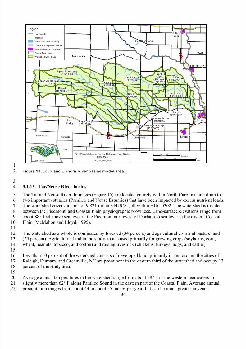
8/13/2019 20 Watersheds Erd
http://slidepdf.com/reader/full/20-watersheds-erd 48/186
1
2
34
56
7
89
10
11
1213
141516
17
1819
20
2122
36
Lincoln
Omaha
Sioux City
SiouxFalls
NorthPlatte
Upper Elkhorn(10220001)
Dismal(10210002)
Lower Elkhorn(10220003)
Upper North Loup(10210006)
South Loup(10210004)
Loup(10210009)
Cedar (10210010)
Calamus(10210008)
Logan(10220004)
Upper Middle Loup(10210001)
Mud(10210005)
Lower Middle Loup(10210003)
Lower North Loup
(10210007)
NorthFork
Elkhorn(10220002)
Nebraska
South Dakota
Iowa
Colorado §̈¦I80
§̈¦I29
GCRP Model Areas - Central Nebraska River BasinsBase Map
NAD_1983_Albers_meters
0 40 8020Kilometers
0 4020Miles ¯
Legend
Hydrography
Interstate
Water (Nat. Atlas Dataset)
US Census Populated Places
Municipalities (pop ≥ 50,000)
County Boundaries
Watershed with HUC8s
Nebraska
Nebraska
Iowa
South DakotaMinnesota
80
Figure 14. Loup and Elkhorn River basins model area.
3.1.13. Tar/Neuse River basins
The Tar and Neuse River drainages (Figure 15) are located entirely within North Carolina, and drain totwo important estuaries (Pamlico and Neuse Estuaries) that have been impacted by excess nutrient loads.
The watershed covers an area of 9,821 mi2 in 8 HUC8s, all within HUC 0302. The watershed is divided
between the Piedmont, and Coastal Plain physiographic provinces. Land-surface elevations range fromabout 885 feet above sea level in the Piedmont northwest of Durham to sea level in the eastern Coastal
Plain (McMahon and Lloyd, 1995).
The watershed as a whole is dominated by forested (34 percent) and agricultural crop and pasture land(29 percent). Agricultural land in the study area is used primarily for growing crops (soybeans, corn,
wheat, peanuts, tobacco, and cotton) and raising livestock (chickens, turkeys, hogs, and cattle.)
Less than 10 percent of the watershed consists of developed land, primarily in and around the cities of
Raleigh, Durham, and Greenville, NC are prominent in the eastern third of the watershed and occupy 13
percent of the study area.
Average annual temperatures in the watershed range from about 58 °F in the western headwaters to
slightly more than 62° F along Pamlico Sound in the eastern part of the Coastal Plain. Average annual precipitation ranges from about 44 to about 55 inches per year, but can be much greater in years
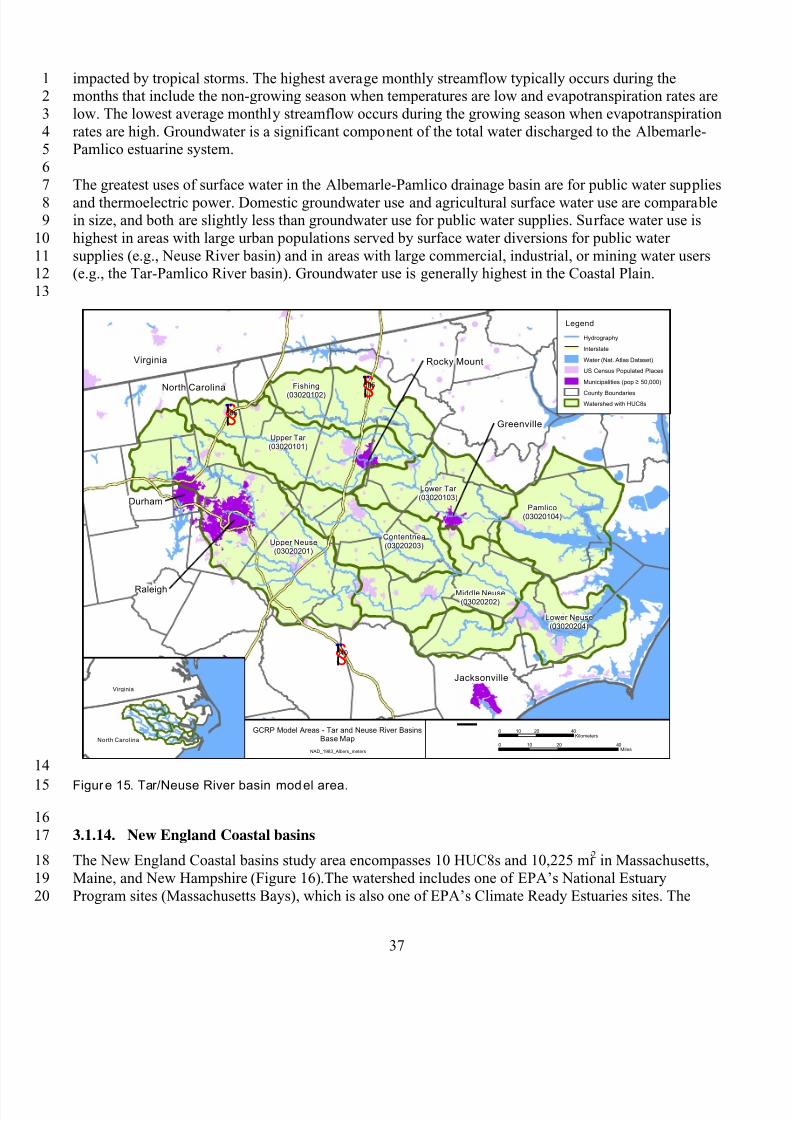
8/13/2019 20 Watersheds Erd
http://slidepdf.com/reader/full/20-watersheds-erd 49/186
12
3
45
6
7
89
10
1112
13
impacted by tropical storms. The highest average monthly streamflow typically occurs during themonths that include the non-growing season when temperatures are low and evapotranspiration rates are
low. The lowest average monthly streamflow occurs during the growing season when evapotranspiration
rates are high. Groundwater is a significant component of the total water discharged to the AlbemarlePamlico estuarine system.
The greatest uses of surface water in the Albemarle-Pamlico drainage basin are for public water supplies
and thermoelectric power. Domestic groundwater use and agricultural surface water use are comparablein size, and both are slightly less than groundwater use for public water supplies. Surface water use is
highest in areas with large urban populations served by surface water diversions for public water
supplies (e.g., Neuse River basin) and in areas with large commercial, industrial, or mining water users(e.g., the Tar-Pamlico River basin). Groundwater use is generally highest in the Coastal Plain.
14
15
16
17
18
19
20
Virginia
North Carolina
Raleigh
Durham
Rocky Mount
Greenville
Jacksonville
Upper Neuse(03020201)
Upper Tar (03020101)
Pamlico(03020104)
Lower Neuse(03020204)
Fishing
(03020102)
Middle Neuse(03020202)
Contentnea(03020203)
Lower Tar (03020103)
§̈¦I85
§̈¦I40
§̈¦I95
GCRP Model Areas - Tar and Neuse River BasinsBase Map
NAD_1983_Albers_meters
0 20 4010Kilometers
0 20 4010Miles ¯
Legend
Hydrography
Interstate
Water (Nat. Atlas Dataset)
US Census Populated Places
Municipalities (pop ≥ 50,000)
County Boundaries
Watershed with HUC8s
Virginia
North Carolina
Figure 15. Tar/Neuse River basin model area.
3.1.14. New England Coastal basins
The New England Coastal basins study area encompasses 10 HUC8s and 10,225 mi2 in Massachusetts,
Maine, and New Hampshire (Figure 16).The watershed includes one of EPA’s National Estuary
Program sites (Massachusetts Bays), which is also one of EPA’s Climate Ready Estuaries sites. The
37
8/13/2019 20 Watersheds Erd
http://slidepdf.com/reader/full/20-watersheds-erd 50/186
12
3
45
6
7
89
10
1112
13
1415
16
1718
1920
entire model area is in the New England Physiographic Province. Elevations in the watershed rangefrom sea level along the coast to greater than 6,000 ft in the White Mountains of New Hampshire.
Average annual precipitation in the watershed ranges from 40 to 50 inches, with higher amounts in themountainous regions – up to 100 inches per year at the summit of Mount Washington. About one-half of
this precipitation becomes surface runoff. Average annual air temperature varies from about 43o F in the
north to about 50o F in the south.
Most of the rivers in this watershed originate in mountainous forested areas with headwaters defined by
fast-flowing water with cobble and boulder-bottom streams. Flow in these rivers is generally regulated
by upstream lakes, reservoirs, flood-control dams, and power plants. The watershed also contains a largenumber of natural lakes, many of which are enlarged and controlled by dams.
The land uses in the watershed are approximately 64 percent forested; 16 percent residential,commercial, and industrial; and 6 percent agricultural. Cities include Boston, MA, Portland, ME,
Worcester, MA, and a variety of smaller cities near the Boston area. Major industries include light
manufacturing, pulp and paper production, silviculture, hydroelectric-power generation, tourism, andseasonal recreation.
38
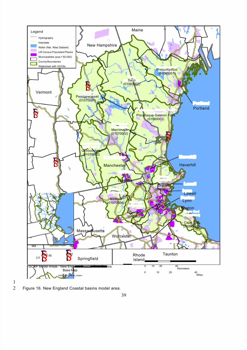
8/13/2019 20 Watersheds Erd
http://slidepdf.com/reader/full/20-watersheds-erd 51/186
1
39
2
New Hampshire
Vermont
Maine
Massachusetts
RhodeIsland
t
Saco(01060002)
Presumpscot(01060001)
Merrimack(01070002)
Charles(01090001)
Pemigewasset(01070001)
Piscataqua-Salmon Falls(01060003)
Contoocook(01070003)
Concord(01070005)
Nashua(01070004)
Cape Cod(01090002)
Taunton
Boston
Nashua
Haverhill
Worcester
Manchester
Springfield
Lynn
Lowell
Portland
§̈¦I91
§̈¦I95
§̈¦I93
§̈¦I89
§̈¦I90 §̈¦I391
GCRP Model Areas - New England Coastal River BasinsBase Map
NAD_1983_Albers_meters
0 20 4010Miles ¯
Legend
Hydrography
Interstate
Water (Nat. Atlas Dataset)
US Census Populated Places
Municipalities (pop ≥ 50,000)
County Boundaries
Watershed with HUC8s
CT
MENH
MA
VT
RI
0 20 4010Kilometers
Figure 16. New England Coastal basins model area.
8/13/2019 20 Watersheds Erd
http://slidepdf.com/reader/full/20-watersheds-erd 52/186
1
23
4
56
789
10
11
1213
14
1516
17
1819
20
2122
23
24
2526
27
28
2930
3132
33
34
3536
3738
3.1.15. Powder/Tongue River basin
The Powder River and Tongue River are major tributaries to the Yellowstone River, which in turn is partof the Missouri River system on the east side of the Rocky Mountains. The model study area consists of
almost 19,000 mi2
in Montana and Wyoming and consists of 12 HUC8s in HUC 1009 (Figure 17).
The watershed lies in parts of the Great Plains, Middle Rocky Mountains, Wyoming Basin, and
Northern Rocky Mountains physiographic provinces (Zelt et al., 1999). Elevation ranges from over13,000 ft on the crest of the Big Horn Range to less than 3,000 ft at the confluence of the Powder andYellowstone Rivers. This large elevation range has important impacts on climate in the watershed,
which ranges from cold and moist in the mountainous areas to temperate and semiarid in the plains
areas. Mean annual temperatures range from less than 32° F at the highest elevations to about 50° F
along the river valleys in Montana. Annual temperature extremes range from about -40° F during thewinter to hotter than 100° F during the summer. Mean annual precipitation ranges from about 12 inches
in the plains to more than 35 inches at high elevations. Snowfall composes a substantial part of annual
precipitation in most years.
Streams in the mountainous areas of the basin generally are perennial and derived primarily from
snowmelt runoff. Most streams originating in the plains areas of the basin are ephemeral, flowing onlyas a result of local snowmelt or intense rainstorms. In some subbasins, where irrigated agriculture is a
major land use, most of the streamflow results from agricultural return flow and sustained base flows.
Rangeland is the dominant land cover (85 percent of the watershed). Cropland and pasture compose less
than 2 percent of the watershed. Silviculture is another important land use activity and forests cover
about 10 percent of the model study area. The watershed is sparsely populated and developed land
accounts for only 0.5 percent of the watershed.
In addition to agriculture, silviculture, and urban uses, other important land uses in the watershed
include metals and coal mining and hydrocarbon production. One of the nation’s largest natural gas
fields lies in the watershed and production from the low-sulfur coal beds in the Powder River basin isincreasing rapidly in response to the demand for low-sulfur steam coal by electric utility consumers. All
of the active coal mines in the watershed are surface (strip) mines.
There are no major storage reservoirs in the watershed, although the Tongue River is impounded near
the state line. However, hundreds of small impoundments for water supply, recreation, power, and flood
control have been constructed in the watershed.
40

8/13/2019 20 Watersheds Erd
http://slidepdf.com/reader/full/20-watersheds-erd 53/186
1
2
41
Wyoming
Montana
Lame Deer
An telope Hill s
West River
Gillette
Billings
Lower Tongue
(10090102)
Upper Tongu e
(10090101)
Upper Powder
(10090202)
Little
Powder
(10090208)
Clear
(10090206)
Salt
(10090204)
Lower
Powder
(10090209)
Mizpah
(10090210)
Middle
Powder (10090207)
Crazy
Woman(10090205)
South Fork
Powder
(10090203)
Middle
Fork
Powder
(10090201)
§̈¦I94
§̈¦I90
§̈¦I25
GCRP Model Areas - Yellowstone River BasinsBase Map
NAD_1983_Albers_meters
0 30 6015Miles ¯
Legend
Hydrography
Interstate
Water (Nat. Atlas Dataset)
US Census Populated Places
Municipalities (pop ≥ 50,000)
County Boundaries
Watershed with HUC8s
Wyoming
Montana
0 30 6015Kilometers
Figure 17. Tongue and Powder River basins model area.
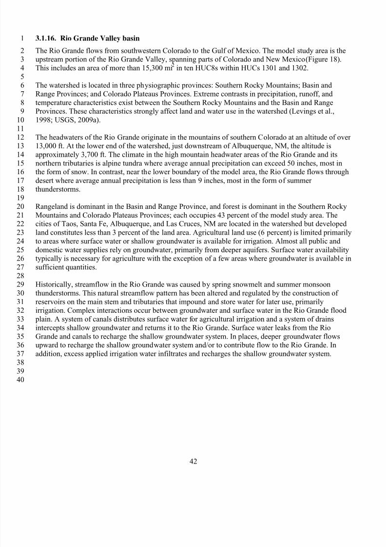
8/13/2019 20 Watersheds Erd
http://slidepdf.com/reader/full/20-watersheds-erd 54/186
1
23
4
56
789
10
11
1213
14
1516
17
1819
20
2122
23
24
2526
27
28
2930
3132
33
34
3536
37
38
39
40
3.1.16. Rio Grande Valley basin
The Rio Grande flows from southwestern Colorado to the Gulf of Mexico. The model study area is theupstream portion of the Rio Grande Valley, spanning parts of Colorado and New Mexico (Figure 18).
This includes an area of more than 15,300 mi2 in ten HUC8s within HUCs 1301 and 1302.
The watershed is located in three physiographic provinces: Southern Rocky Mountains; Basin and
Range Provinces; and Colorado Plateaus Provinces. Extreme contrasts in precipitation, runoff, andtemperature characteristics exist between the Southern Rocky Mountains and the Basin and RangeProvinces. These characteristics strongly affect land and water use in the watershed (Levings et al.,
1998; USGS, 2009a).
The headwaters of the Rio Grande originate in the mountains of southern Colorado at an altitude of over13,000 ft. At the lower end of the watershed, just downstream of Albuquerque, NM, the altitude is
approximately 3,700 ft. The climate in the high mountain headwater areas of the Rio Grande and its
northern tributaries is alpine tundra where average annual precipitation can exceed 50 inches, most inthe form of snow. In contrast, near the lower boundary of the model area, the Rio Grande flows through
desert where average annual precipitation is less than 9 inches, most in the form of summer
thunderstorms.
Rangeland is dominant in the Basin and Range Province, and forest is dominant in the Southern Rocky
Mountains and Colorado Plateaus Provinces; each occupies 43 percent of the model study area. Thecities of Taos, Santa Fe, Albuquerque, and Las Cruces, NM are located in the watershed but developed
land constitutes less than 3 percent of the land area. Agricultural land use (6 percent) is limited primarily
to areas where surface water or shallow groundwater is available for irrigation. Almost all public and
domestic water supplies rely on groundwater, primarily from deeper aquifers. Surface water availabilitytypically is necessary for agriculture with the exception of a few areas where groundwater is available in
sufficient quantities.
Historically, streamflow in the Rio Grande was caused by spring snowmelt and summer monsoonthunderstorms. This natural streamflow pattern has been altered and regulated by the construction of
reservoirs on the main stem and tributaries that impound and store water for later use, primarilyirrigation. Complex interactions occur between groundwater and surface water in the Rio Grande flood
plain. A system of canals distributes surface water for agricultural irrigation and a system of drains
intercepts shallow groundwater and returns it to the Rio Grande. Surface water leaks from the Rio
Grande and canals to recharge the shallow groundwater system. In places, deeper groundwater flowsupward to recharge the shallow groundwater system and/or to contribute flow to the Rio Grande. In
addition, excess applied irrigation water infiltrates and recharges the shallow groundwater system.
42
8/13/2019 20 Watersheds Erd
http://slidepdf.com/reader/full/20-watersheds-erd 55/186
1
2
43
§̈¦25
Colorado
§̈¦40
Jemez
(13020202)
New Mexico
Rio Chama(13020102)
San Lu is
(13010003)
Upper Rio Grande
(13020101)
Saguache
(13010004)
Alamosa-Trin chera
(13010002)
Rio Grande-
Santa Fe
(13020201)
Rio Grande-
Albu querque
(13020203)
Rio Grande
Headwaters
(13010001)
Conejos(13010005)
Albuquerque
Alamo
Santa Fe
Angel Fir e
GrantsEncinal
Socorro
Cedar GroveMesita
Glorieta
Taos
Espanola
Magdalena
Blanca
GCRP Model Areas - Rio Grande River BasinBase Map
NAD_1983_Albers_meters
0 4020Miles ¯
Legend
Hydrography
Interstate
Water (Nat. Atlas Dataset)
US Census Populated Places
Municipalities (pop ≥ 50,000)
County Boundaries
Watershed with HUC8s
Colorado
New Mexico
0 40 8020Kilometers
80
Figure 18. Rio Grande Valley basin model area.
8/13/2019 20 Watersheds Erd
http://slidepdf.com/reader/full/20-watersheds-erd 56/186
1
2
3
4
56
789
10
11
1213
14
1516
17
1819
20
2122
23
24
2526
27
28
2930
31
3233
3.1.17. Sacramento River basin
The Sacramento River in northern California is vital to the state's economy and for providing freshwater
flow to the San Francisco Bay. Lake Shasta impounds the mainstem and is subject to complex
operational rules. This study considers only the portion of the Sacramento River basin from Lake Shastato just before the confluence with the Feather River (Figure 19). Information was not available for this
study to represent changes in reservoir operations in response to climate change. Lake Shasta outflowtime series were thus considered a fixed upstream boundary condition. The resulting model areacontains over 8,300 mi
2 in 11 HUC8s, all within HUC 1802.
The average annual precipitation in the entire watershed ranges from 18 in/yr near Sacramento to about
75 in/yr at the highest elevations, mostly occurring from November through March. Snow melt is themajor source of flow for the rivers of the watershed.
The Sacramento River is a major source of drinking water for residents of northern and southernCalifornia, and is a principal source of irrigation water for Sacramento and San Joaquin Valley farmers.
The land uses in the valley portion of the Sacramento River basin model area are dominated by
agriculture (31 percent pasture/hay, 21 percent cultivated). The Sacramento Valley supports a diverseagricultural economy, much of which depends on the availability of irrigation water. Dairy products and
crops including rice, fruits and nuts, tomatoes, sugar beets, corn, alfalfa, and wheat are important
agricultural commodities. The larger cities in the watershed, located in the Sacramento Valley, includeChico and Redding, with developed land occupying a little over 4 percent of the watershed. The
remaining areas are primarily forest and range.
Agriculture is the largest consumer of water in the basin. Up to about 6 million acre-feet per year ofwater also is exported from the basin, principally to areas in southern California. Part of the runoff from
winter rains and spring snowmelt is stored in reservoirs and released during the normally dry summer
months. Most of the water supplies are derived from these reservoirs. The water is mainly used to
provide irrigation water to the Sacramento and San Joaquin Valley agricultural communities, and to provide drinking water to Central Valley residents and residents of southern California, and to protect
water quality of the delta of the Sacramento and San Joaquin Rivers.
44
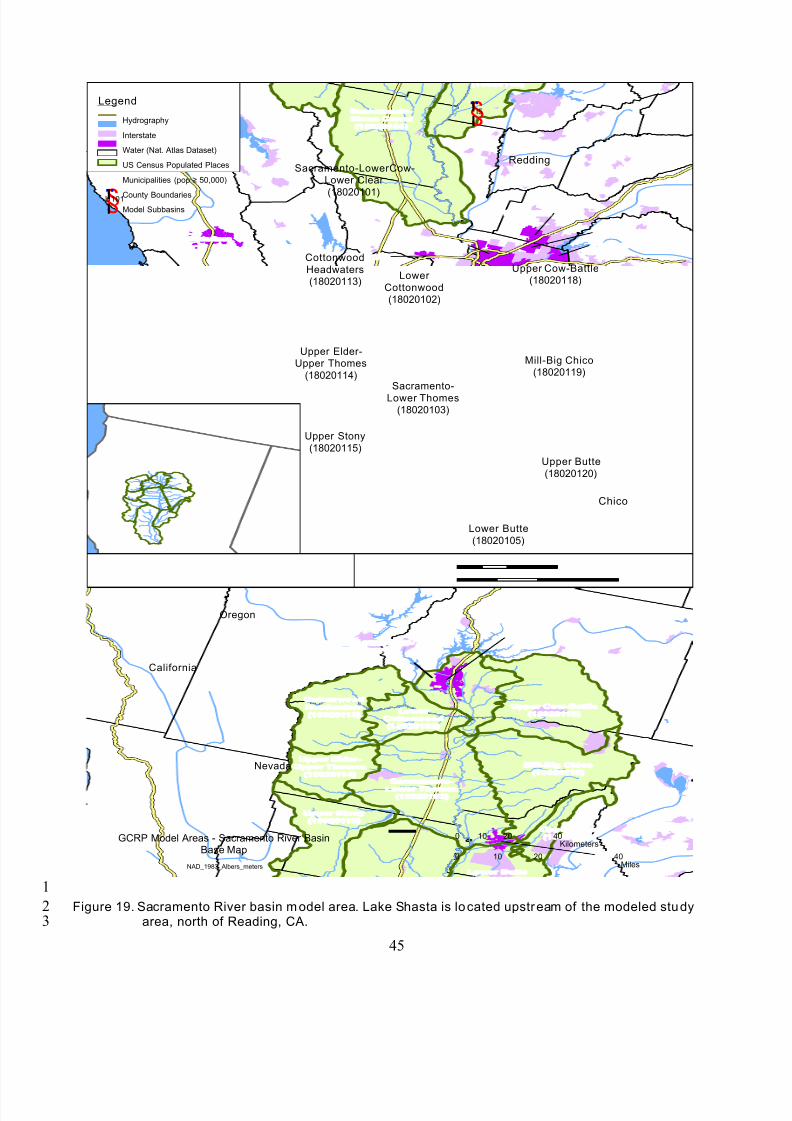
8/13/2019 20 Watersheds Erd
http://slidepdf.com/reader/full/20-watersheds-erd 57/186
1
23
45
P ifi
Sacramento
§̈¦U101
§̈¦I80
§̈¦I505
§̈¦I5
Redding
Chico
Santa Rosa
Roseville
Folsom
Davis
Citrus Heights
Mill-Big Chico(18020119)
Sacramento-Stone Corral
(18020104)
Upper Stony
(18020115)
Sacramento-
Lower Thomes(18020103)
Upper Cow-Battle(18020118)
Lower Butte
(18020105)
Cottonwood
Headwaters(18020113)
Lower
Cottonwood(18020102)
Sacramento-LowerCow-Lower Clear
(18020101)
Upper Elder-Upper Thomes
(18020114)
Upper Butte
(18020120)
GCRP Model Areas - Sacramento River BasinBase Map
NAD_1983_Albers_meters
0 20 4010Miles ¯
Legend
Hydrography
Interstate
Water (Nat. Atlas Dataset)
US Census Populated Places
Municipalities (pop ≥ 50,000)
County BoundariesModel Subbasins
0 20 4010Kilometers
Oregon
California
Nevada
Figure 19. Sacramento River basin model area. Lake Shasta is located upstream of the modeled studyarea, north of Reading, CA.
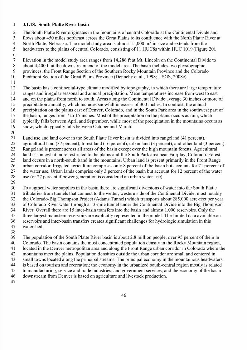
8/13/2019 20 Watersheds Erd
http://slidepdf.com/reader/full/20-watersheds-erd 58/186
1
23
4
56
789
10
11
1213
14
1516
17
1819
2021
2223
24
25
2627
28
2930
31
3233
34
35
3637383940
41
4243
44
45
46
47
3.1.18. South Platte River basin
The South Platte River originates in the mountains of central Colorado at the Continental Divide andflows about 450 miles northeast across the Great Plains to its confluence with the North Platte River at
North Platte, Nebraska. The model study area is almost 15,000 mi2
in size and extends from the
headwaters to the plains of central Colorado, consisting of 11 HUC8s within HUC 1019 (Figure 20).
Elevation in the model study area ranges from 14,286 ft at Mt. Lincoln on the Continental Divide toabout 4,400 ft at the downstream end of the model area. The basin includes two physiographic provinces, the Front Range Section of the Southern Rocky Mountain Province and the Colorado
Piedmont Section of the Great Plains Province (Dennehy et al., 1998; USGS, 2008c).
The basin has a continental-type climate modified by topography, in which there are large temperatureranges and irregular seasonal and annual precipitation. Mean temperatures increase from west to east
and on the plains from north to south. Areas along the Continental Divide average 30 inches or more of
precipitation annually, which includes snowfall in excess of 300 inches. In contrast, the annual precipitation on the plains east of Denver, Colorado, and in the South Park area in the southwest part of
the basin, ranges from 7 to 15 inches. Most of the precipitation on the plains occurs as rain, which
typically falls between April and September, while most of the precipitation in the mountains occurs assnow, which typically falls between October and March.
Land use and land cover in the South Platte River basin is divided into rangeland (41 percent),
agricultural land (37 percent), forest land (16 percent), urban land (3 percent), and other land (3 percent).Rangeland is present across all areas of the basin except over the high mountain forests. Agricultural
land is somewhat more restricted to the plains and the South Park area near Fairplay, Colorado. Forest
land occurs in a north-south band in the mountains. Urban land is present primarily in the Front Range
urban corridor. Irrigated agriculture comprises only 8 percent of the basin but accounts for 71 percent ofthe water use. Urban lands comprise only 3 percent of the basin but account for 12 percent of the water
use (or 27 percent if power generation is considered an urban water use).
To augment water supplies in the basin there are significant diversions of water into the South Platte
tributaries from tunnels that connect to the wetter, western side of the Continental Divide, most notably
the Colorado-Big Thompson Project (Adams Tunnel) which transports about 285,000 acre-feet per yearof Colorado River water through a 13-mile tunnel under the Continental Divide into the Big Thompson
River. Overall there are 15 inter-basin transfers into the basin and almost 1,000 reservoirs. Only the
three largest mainstem reservoirs are explicitly represented in the model. The limited data available on
reservoirs and inter-basin transfers creates significant challenges for hydrologic simulation in thiswatershed.
The population of the South Platte River basin is about 2.8 million people, over 95 percent of them inColorado. The basin contains the most concentrated population density in the Rocky Mountain region,
located in the Denver metropolitan area and along the Front Range urban corridor in Colorado where the
mountains meet the plains. Population densities outside the urban corridor are small and centered insmall towns located along the principal streams. The principal economy in the mountainous headwaters
is based on tourism and recreation; the economy in the urbanized south-central region mostly is related
to manufacturing, service and trade industries, and government services; and the economy of the basin
downstream from Denver is based on agriculture and livestock production.
46
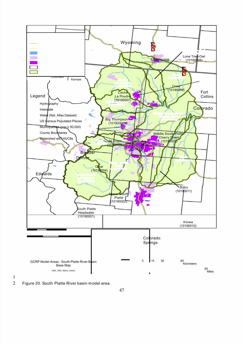
8/13/2019 20 Watersheds Erd
http://slidepdf.com/reader/full/20-watersheds-erd 59/186
1
2
47
Cheyenne
Kiowa(10190010)
Denver
ColoradoSprings
Edwards
FortCollins
Boulder
Colorado
Wyoming
Bijou(10190011)
Middle South Platte-Cherry Creek
(10190003)
Upper SouthPlatte
(10190002)
Crow(10190009)
St. Vrain(10190005)
CacheLa Poudre(10190007)
South PlatteHeadwater (10190001)
Clear (10190004)
Big Thompson(10190006)
Lone Tree-Owl
(10190008)
§̈¦I25
§̈¦I80
GCRP Model Areas - South Platte River BasinBase Map
NAD_1983_Albers_meters ¯
Colorado
NebraskaWyoming
Kansas
Wyo min g
0 3015Miles
Legend
Hydrography
Interstate
Water (Nat. Atlas Dataset)
US Census Populated Places
Municipalities (pop ≥ 50,000)
County Boundaries
Watershed with HUC8s
0 30 6015Kilometers
60
Figure 20. South Platte River basin model area.
8/13/2019 20 Watersheds Erd
http://slidepdf.com/reader/full/20-watersheds-erd 60/186
1
2
3
4
56
789
10
11
1213
14
1516
17
1819
20
2122
23
24
2526
27
28
2930
3132
33
34
3536
37
3839
40
3.1.19. Trinity River basin
The Trinity River basin is located in east central Texas. It extends on a southeast diagonal, from
immediately south of the Oklahoma-Texas border to the Trinity Bay at the Gulf of Mexico. The model
study area encompasses a little over 13,000 mi2
in 12 HUC8s in HUC 1203 (Figure 21). The watershedis dissected by alternate bands of rolling, treeless prairies, smooth to slightly rolling prairies, rolling
timbered hills, and a relatively flat coastal plain. The watershed slopes gradually from about 1,200 ftabove sea level in the northwest, to about 600 ft mid-basin, and on to sea level in the southeasternsection of the area, at Trinity Bay (Land et al., 1998; Ulery et al., 1993).
Past and current human activities, including construction of reservoirs, urbanization, farming, ranching,
and oil and gas production, have greatly altered the natural environment in the Trinity River basin.Approximately 37 percent of the watershed is cropland or pasture. Major crops include corn, cotton,
peanuts, sorghum, soybeans, rice, and wheat. Wheat and cotton are dry cropland crops, while rice is an
irrigated crop. Forest and wetlands represent about 33 percent of the watershed and developed landmakes up about 19 percent of the watershed. The population in the watershed is mainly clustered in the
Dallas-Fort Worth metropolitan area, with a few secondary population clusters (Denton, McKinney,
Corsicana, and Waxahachie).
The climate of the basin is described as modified-marine, subtropical-humid, having warm summers and
a predominant onshore flow of tropical maritime air from the Gulf of Mexico. Precipitation variesconsiderably across the watershed. Average annual precipitation ranges from less than 27 inches in the
northwest part of the watershed to greater than 52 inches in the southeast. On average, the watershed
experiences a winter surplus and a summer deficiency of precipitation. Average annual temperature is
fairly uniform throughout the basin, ranging from about 69° F in the southeastern area of the watershedto about 65° F in the northwest.
There are 22 large reservoirs in the Trinity River basin and hundreds of smaller reservoirs, mostly flood
control structures. Reservoirs have been built to retain runoff on all major tributaries and the mainstemof the Trinity River. Diversions move water within the basin and to and from adjacent river basins. The
largest interbasin diversion is out of the basin, from the Trinity River below Livingston Reservoir to theHouston metropolitan area. There are numerous other inter- and intrabasin diversions.
The largest consumptive use in the watershed is domestic with the majority being used in Dallas and
Tarrant counties because of their large populations. Surface water, almost entirely from reservoirs,supplies more than 90 percent of the water used in the basin. Groundwater is used for municipal and
domestic supply in some of the smaller towns and in rural areas. Transfers of water, from the adjoining
basins and from reservoirs below Dallas and Fort Worth, are required to meet the needs of the Dallas-Fort Worth area. Relatively little water is used for irrigating crops.
48
8/13/2019 20 Watersheds Erd
http://slidepdf.com/reader/full/20-watersheds-erd 61/186
1
2
49
CollegeStation
Houston
Longview
Dallas
Ft. Worth
WichitaFalls
Waco
§̈¦I10
§̈¦I20
§̈¦I30
§̈¦I45
§̈¦I35
§̈¦I410
§̈¦U281
Texas
Oklahoma
Lower TrinityKickapoo
(12030202)
Elm Fork
Trinity(12030103)
Cedar (12030107)
Upper Trinity
(12030105)
Lower Trinity-Tehuacana(12030201)
Upper WestFork Trinity(12030101)
Chambers
(12030109)
East ForkTrinity
(12030106)
Richland(12030108)
Denton(12030104)
Lower WestFork Trinity(12030102)
Lower Trinity
(12030203)
GCRP Model Areas - Trinity River BasinBase Map
NAD_1983_Albers_meters
0 30 6015Miles ¯
Legend
Hydrography
Interstate
Water (Nat. Atlas Dataset)
US Census Populated Places
Municipalities (pop≥
50,000)County Boundaries
Watershed with HUC8s
Texas
Oklahoma
0 30 6015Kilometers
Figure 21. Trinit y River basin model area.
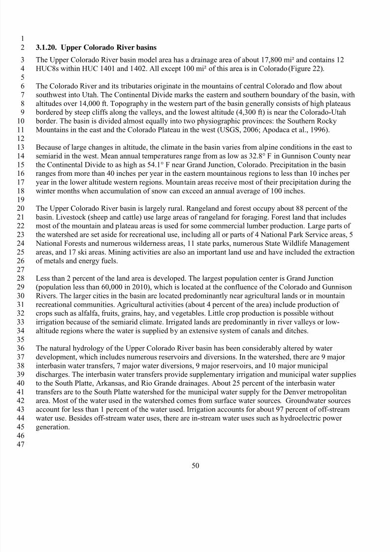
8/13/2019 20 Watersheds Erd
http://slidepdf.com/reader/full/20-watersheds-erd 62/186
1
2
3
4
56
789
10
11
1213
14
1516
17
1819
20
2122
23
24
2526
27
28
2930
3132
33
34
3536
37
3839
404142
43
44
4546
47
3.1.20. Upper Colorado River basins
The Upper Colorado River basin model area has a drainage area of about 17,800 mi² and contains 12
HUC8s within HUC 1401 and 1402. All except 100 mi² of this area is in Colorado (Figure 22).
The Colorado River and its tributaries originate in the mountains of central Colorado and flow about
southwest into Utah. The Continental Divide marks the eastern and southern boundary of the basin, withaltitudes over 14,000 ft. Topography in the western part of the basin generally consists of high plateaus bordered by steep cliffs along the valleys, and the lowest altitude (4,300 ft) is near the Colorado-Utah
border. The basin is divided almost equally into two physiographic provinces: the Southern Rocky
Mountains in the east and the Colorado Plateau in the west (USGS, 2006; Apodaca et al., 1996).
Because of large changes in altitude, the climate in the basin varies from alpine conditions in the east to
semiarid in the west. Mean annual temperatures range from as low as 32.8° F in Gunnison County near
the Continental Divide to as high as 54.1° F near Grand Junction, Colorado. Precipitation in the basinranges from more than 40 inches per year in the eastern mountainous regions to less than 10 inches per
year in the lower altitude western regions. Mountain areas receive most of their precipitation during the
winter months when accumulation of snow can exceed an annual average of 100 inches.
The Upper Colorado River basin is largely rural. Rangeland and forest occupy about 88 percent of the
basin. Livestock (sheep and cattle) use large areas of rangeland for foraging. Forest land that includesmost of the mountain and plateau areas is used for some commercial lumber production. Large parts of
the watershed are set aside for recreational use, including all or parts of 4 National Park Service areas, 5
National Forests and numerous wilderness areas, 11 state parks, numerous State Wildlife Management
areas, and 17 ski areas. Mining activities are also an important land use and have included the extractionof metals and energy fuels.
Less than 2 percent of the land area is developed. The largest population center is Grand Junction
(population less than 60,000 in 2010), which is located at the confluence of the Colorado and GunnisonRivers. The larger cities in the basin are located predominantly near agricultural lands or in mountain
recreational communities. Agricultural activities (about 4 percent of the area) include production ofcrops such as alfalfa, fruits, grains, hay, and vegetables. Little crop production is possible without
irrigation because of the semiarid climate. Irrigated lands are predominantly in river valleys or low-
altitude regions where the water is supplied by an extensive system of canals and ditches.
The natural hydrology of the Upper Colorado River basin has been considerably altered by water
development, which includes numerous reservoirs and diversions. In the watershed, there are 9 major
interbasin water transfers, 7 major water diversions, 9 major reservoirs, and 10 major municipaldischarges. The interbasin water transfers provide supplementary irrigation and municipal water supplies
to the South Platte, Arkansas, and Rio Grande drainages. About 25 percent of the interbasin watertransfers are to the South Platte watershed for the municipal water supply for the Denver metropolitanarea. Most of the water used in the watershed comes from surface water sources. Groundwater sources
account for less than 1 percent of the water used. Irrigation accounts for about 97 percent of off-stream
water use. Besides off-stream water uses, there are in-stream water uses such as hydroelectric power
generation.
50
8/13/2019 20 Watersheds Erd
http://slidepdf.com/reader/full/20-watersheds-erd 63/186
1
2
51
Denver
ColoradoSprings
GrandJunction
Edwards
FortCollins
Boulder
Loveland
HighlandsRanch
Colorado Headwaters(14010001)
Upper Gunnison(14020002)
Colorado Headwaters-Plateau
(14010005)Roaring Fork
(14010004)
Lower Gunnison(14020005)
Eagle(14010003)
Tomichi(14020003)
Blue(14010002)
Uncompahgre(14020006)
East-Taylor
(14020001)
North ForkGunnison(14020004)
Parachute-Roan
(14010006)
Colorado
Utah
§̈¦I70
GCRP Model Areas - Upper Colorado River BasinBase Map
NAD_1983_Albers_meters
0 30 6015Kilometers
0 3015Miles ¯
Legend
Hydrography
Interstate
Water (Nat. Atlas Dataset)
US Census Populated Places
Municipalities (pop ≥ 50,000)
County Boundaries
Watershed with HUC8s
Colorado
Utah
60
Figure 22. Upper Colorado River basin model area.
8/13/2019 20 Watersheds Erd
http://slidepdf.com/reader/full/20-watersheds-erd 64/186
5
10
15
20
25
30
35
1
2
34
67
8
9
11
12
1314
1617
18
19
21
2223
24
2627
28
29
31
3233
34
36
37
38
4. MODELING APPROACH
This study involves application of dynamic watershed models to simulate the watershed response
to potential changes in climate, changes in urban development, and the combined effects ofchanges in climate change and urban development. Watershed modeling was conducted using
two watershed models, Hydrologic Simulation Program – FORTRAN (HSPF; Bicknell et al.
2001) and Soil and Water Assessment Tool (SWAT; Neitsch et al., 2005). The SWAT modelwas applied in all 20 study areas. In a subset of five of the 20 sites (hereafter referred to as “Pilot
Sites”), simulations were also conducted independently using HSPF. Simulations focus on
changes in streamflow, nutrient (nitrogen and phosphorus) and sediment loads.
A watershed model is a useful tool for providing a quantitative linkage between external forcing
and in-stream response. It is essentially a series of algorithms applied to watershed
characteristics and meteorological data to simulate naturally occurring, land-based processesover an extended period, including hydrology and pollutant transport. Many watershed models
are also capable of simulating in-stream processes. After a model has been set up and calibrated
for a watershed, it can be used to quantify the existing loading of pollutants from subbasins orfrom land use categories and can also be used to assess the effects of a variety of management
scenarios.
The results of watershed assessment are shaped by the characteristics of the watershed model
that serves to translate climate forcing into hydrologic and water quality responses. Two
watershed models were selected for initial application to the five pilot study sites: HydrologicalSimulation Program – FORTRAN (HSPF) (Bicknell et al., 2001) and Soil Water Assessment
Tool (SWAT) (Neitsch et al., 2005). These models were selected because they met the following
criteria:
•Dynamic simulation with a sub-daily or daily time step to give an indication of changes infrequency of extreme events
• Process-based, but at a level that model parameters can be easily identified from available data
• Able to simulate water quality responses
• Widely used and accepted for hydrologic and water quality applications
• In the public domain to enable ready replication of results
Application of both HSPF and SWAT to the five pilot watersheds allowed assessment of thevariability associated with use of different watershed models in simulating watershed response to
climate change. The two watershed models are described below. The rationale for selecting theSWAT model for use in non-pilot watersheds is discussed in Section 6.1 (Comparison ofModels).
52
8/13/2019 20 Watersheds Erd
http://slidepdf.com/reader/full/20-watersheds-erd 65/186
1
2
3
4
56
7
89
10
1112
13
14
15
16
17
1819
20
21
2223
24
25
2627
2829
30
31
3233
34
3536
373839
40
4142
43
44
4.1. MODEL BACKGROUND
4.1.1. HSPF
The Hydrological Simulation Program – FORTRAN (HSPF; Bicknell et al., 2001) is a
comprehensive, dynamic watershed and receiving water quality modeling framework that was
originally developed in the mid-1970s. During the past several decades, it has been used todevelop hundreds of EPA-approved Total Maximum Daily Loads (TMDLs), and it is generally
considered among the most advanced hydrologic and watershed loading models available. The
hydrologic portion of HSPF is based on the Stanford Watershed Model (Crawford and Linsley,1966), which was one of the pioneering watershed models developed in the 1960s. The HSPF
framework is developed modularly with many different components that can be assembled in
different ways, depending on the objectives of a project. The model includes three majormodules:
• PERLND for simulating watershed processes on pervious land areas
• IMPLND for simulating processes on impervious land areas
• RCHRES for simulating processes in streams and vertically mixed lakes
All three of these modules include many subroutines that calculate the various hydrologic and
water quality processes in the watershed. Many options are available for both simplified and
complex process formulations.
HSPF models hydrology as a water balance in multiple surface and subsurface layers and is
typically implemented in large watersheds at an hourly time step. The water balance is simulated
based on Philip’s infiltration (Bicknell et al., 2001, 2005) coupled with multiple surface andsubsurface stores (interception storage, surface storage, upper zone soil storage, lower zone soil
storage, active groundwater, inactive (deep) groundwater). Potential evapotranspiration (PET) is
externally specified to the model.
Sediment erosion in HSPF uses a method that is formally similar to, but distinct from the USLE
sediment-detachment approach coupled with transport capacity based on overland flow. Nutrients may be simulated at varying levels of complexity, but are most typically represented
by either buildup/washoff or sediment potency approaches on the land surface coupled with user-
specified monthly concentrations in interflow and groundwater.
Spatially, the watershed is divided into a series of subbasins representing the drainage areas that
contribute to each of the stream reaches. The stream network (RCHRES) links the surface runoff
and groundwater flow contributions from each of the land segments and sub-basins and routesthem through waterbodies. The stream model includes precipitation and evaporation from the
water surfaces as well as flow contributions from the watershed, tributaries, and upstream streamreaches. It also simulates a full range of stream sediment and nutrient processes, includingdetailed representations of scour, deposition, and algal growth.
The version of HSPF used in this study is WinHSPF as distributed with BASINS version 4.0.WinHSPF is a Windows interface to HSPF and is a component of the EPA’s Better Assessment
Science Integrating point and Nonpoint Sources (BASINS) Version 4.0 (U.S. EPA, 2009b,
2009c). WinHSPF itself is a user interface to HSPF that assists the user in building User Control
53
8/13/2019 20 Watersheds Erd
http://slidepdf.com/reader/full/20-watersheds-erd 66/186
1
2
34
5
67
8
9
1011
12
1314
15
16
17
1819
20
2122
23
2425
26
27
2829
30
3132
33
3435
36
3738
3940
4142
43
4445
46
Input (UCI) files (containing model input parameters) from GIS data (Duda et al., 2001). After
the UCI file is built, WinHSPF is used to view, understand, and modify the model representation
of a watershed. HSPF can be run from within WinHSPF. The actual model executable enginedistributed with BASINS is called WinHSPFLt, which can be run in batch mode independent of
the BASINS/WinHSPF interface. The model code for HSPF is stable and well-documented.
Detailed descriptions of the model theory and user control input are provided in Bicknell et al.,(2001, 2005).
WinHSPF also provides access to the Climate Assessment Tool (CAT), which is a component of
BASINS 4.0. BASINS CAT facilitates watershed-based assessments of the potential effects ofclimate variability and change on water and watershed systems (namely streamflow and pollutant
loads) using the HSPF model (U.S. EPA, 2009b, 2009c). BASINS CAT is capable of creating
climate change scenarios that allow users to assess a wide range of what if questions related toclimate change.
4.1.2. SWAT
The Soil Water Assessment Tool (SWAT, version 2005) model (Neitsch et al., 2005) was also
applied to the watersheds to simulate flow and nitrogen, phosphorus and sediment loads. SWATwas developed by the U.S. Department of Agriculture to simulate the effect of land management
practices on water, sediment, and agricultural chemical yields in large, complex watersheds with
varying soils, land use, and management conditions over long periods of time (Neitsch et al.,2005). SWAT requires data inputs for weather, soils, topography, vegetation, and land use to
model water and sediment movement, nutrient cycling, and numerous other watershed processes.
SWAT is a continuous model appropriate to long-term simulations.
SWAT, as implemented here, employs a curve number approach to estimate surface runoff and
then completes the water balance through simulation of subsurface flows, evapotranspiration,
soil storages, and deep seepage losses. The curve number approach requires a daily time step.PET is typically calculated internally by SWAT based on other weather inputs.
Sediment yield and erosion are calculated by SWAT using the Modified Universal Soil LossEquation (MUSLE) (Williams, 1975). The MUSLE is based on several factors including surface
runoff volume, peak runoff rate, area of hydrologic response unit (HRU), soil erodibility, land
cover and management, support practice, topography, and a coarse fragment factor and implicitlycombines the processes of sediment detachment and delivery. Nutrient load generation and
movement is simulated using overland runoff and subsurface flow.
A key feature of SWAT is the incorporation of an explicit plant growth model, including plant
interactions with water and nutrient stores. The transformation of various nitrogen and phosphorus species is simulated in detail in the soil; however, concentrations of nutrients in
groundwater discharges are user-specified, as in HSPF.
Instream simulation of sediment in SWAT 2005 includes a highly simplified representation of
scour and deposition processes. Nutrient kinetics in receiving waters are based on the numericrepresentation used in the QUAL2E model but implemented only at a daily time step.
54
8/13/2019 20 Watersheds Erd
http://slidepdf.com/reader/full/20-watersheds-erd 67/186
5
10
15
20
25
30
35
40
1
2
34
67
8
9
11
12
1314
16
1718
19
21
22
23
24
26
27
2829
3132
33
34
36
37
38
39
41
An important component of the SWAT model is the weather generator (WXGEN). SWAT
requires daily values of precipitation, maximum and minimum temperature, solar radiation,
relative humidity, and wind speed. The user may read these inputs from a file or generate thevalues using SWAT’s weather generator model based on monthly average data summarized over
a number of years (Neitsch et al., 2005). The weather generator model (Sharpley and Williams,
1990) can be used to generate climatic data or to fill in gaps in weather data. The weathergenerator first independently generates precipitation for the day. Maximum temperature,
minimum temperature, solar radiation, and relative humidity are then generated based on the
presence or absence of rain for the day. Finally, wind speed is generated independently.
The version SWAT used in this study is SWAT2005 as distributed with ArcSWAT 2.1, which
was the most recent stable version of SWAT available at the start of this study. ArcSWAT 2.1 is
an ArcGIS-ArcView extension and a graphical user input interface for the SWAT watershedmodel (TAMU, 2010). As with HSPF, the underlying executable code can be run in batch mode
independent of the user interface. Unlike HSPF, the SWAT code is continuously evolving, with
frequent enhancements and bug fixes. For a detailed description of the version of SWAT used
here, see Neitsch et al. (2005).
4.2. MODEL SETUP
The watershed models were configured to simulate the study areas as a series of hydrologicallyconnected subbasins. Configuration of the models involved subdivision of the watersheds into
modeling units, followed by continuous simulation of flow and water quality for these units
using meteorological, land use, soil, and stream data. The specific pollutants modeled were
nitrogen, phosphorus, and sediment.
Many study areas are highly managed systems influenced by humans including dams, water
transfers and withdrawals, point source discharges and other factors. Given the difficulty
modeling at the large spatial scale in this study, detailed representation of all management wasnot possible. The following assumptions were made to simplify modeling among all 20 study
areas:
• External boundary conditions (where needed), such as upstream inflows and pollutant loads, are
assumed constant.
• Interactions with deep groundwater systems are assumed constant.
• Large-scale shifts in natural cover type in response to climate change are not simulated.
• Point source discharges and water withdrawals are assumed constant at current levels.
• Only large dams that have a significant impact on hydrology at the HUC8 scale are included in
the models. Where these dams are simulated an approximation of current operating rules (using a
target storage approach) is assumed to apply in all future scenarios.
• Human adaptation response to climate change, such as shifts in water use or cropping practices,
are not simulated.
55
8/13/2019 20 Watersheds Erd
http://slidepdf.com/reader/full/20-watersheds-erd 68/186
1
2
34
5
67
8
9
1011
12
1314
15
16
1718
19
2021
22
2324
25
2627
28
2930
31
32
33
34
35
36
3738
394041
42
43
4445
46
Results therefore represent the behavior and potential responses of watersheds to different
change scenarios but should not be considered quantitative forecasts of future conditions.
The modeling effort in this study was extensive and involved multiple modelers. To ensure
consistency of results, a common set of procedures and assumptions was established as follows
(e.g., see appendix A). Both HSPF and SWAT were implemented using a hydrologic responseunit (HRU) approach to upland simulation. An HRU consists of a unique combination of land
use/land cover, soil, and land management practice characteristics, and thus represents areas of
similar hydrologic response. This is the default for SWAT, but is also good practice with HSPF.
Consistent with the broad spatial scale of the models, the land cover component is interpreted toa relatively small number of categories (e.g., forest, wetland, range, grass/pastureland, crop,
developed pervious, low-density impervious, and high-density impervious).
Initial processing took place primarily in ArcGIS for the entire study area. Processed GIS inputs
were then used in ArcSWAT (which runs as an extension in ArcGIS), and imported into
BASINS4 (which uses MapWindow GIS). Spatial data sources are discussed in more detail in
Section 4.2.3. Additional initial setup tasks included:
1. Identification of BASINS4 weather stations in proximity of model watersheds
2. Identification of locations and characteristics of any major reservoirs or neededcalibration points
3. Identification of locations and characteristics of any major features in the watershed
affecting water balance (e.g., diversions, upstream areas not modeled, reaches that loseflow to groundwater). Irrigation was considered only where needed (e.g., Rio Grande)
4. Identification of locations of major point sources
5. Identification of flow gaging station and water quality monitoring station locations6. Modification of subbasin boundaries as needed to accommodate the previous four items
7. Identification of nearest precipitation weather station to each subbasin, and identification
of subbasin assignment for elevation bands and other characteristics (e.g., soil andgeology) that needed to be represented on a regional basis in the models
8. Atmospheric deposition of nitrogen – each model was set up appropriately to model a
constant concentration for wet deposition and a constant load for dry deposition
4.2.1. SWAT Setup Process
SWAT model setup followed directly from the initial setup, using the ArcSWAT extension in
ArcGIS. The following steps were implemented first for the calibration HUC8 subbasins then
repeated for the entire modeled watershed. A detailed description of the SWAT model setup forthe 15 non-pilot watersheds is included in Appendix A.
The first step was watershed delineation. In general, subbasin boundaries and reach hydrographywere defined from NHDPlus catchments (U.S. EPA, 2010), aggregated to approximately the
HUC10 scale. The subbasin and reach shapefiles were imported into the SWAT interface and
subbasin parameters were calculated automatically. The next step was to add major reservoirs in
the watershed. Study sites were selected to minimize the presence of reservoirs to reduce thedifficulty of representing operational rules, and model included only major reservoirs that have a
significant effect on flows at the scale of HUC8s or greater. Inclusion of reservoirs was left to the
56
8/13/2019 20 Watersheds Erd
http://slidepdf.com/reader/full/20-watersheds-erd 69/186
1
2
34
5
67
8
9
1011
12
1314
15
16
1718
19
2021
22
2324
25
2627
28
2930
31
32
3334
35
3637
38
3940
41
42
4344
45
discretion of individual modelers; however, reservoirs included are generally those that drain an
area greater than a single HUC8 and provide a retention time of half a year or greater. If a
reservoir was located at the terminus of the model area it was generally ignored so that the modelrepresented input to, rather than output from, the terminal reservoir.
Only those permitted point sources identified as major facilities (greater than 1 MGD discharge)were included in the model. It was also necessary to define an upstream boundary condition
“point source” for some watersheds.
Land use for the model comes from the 2001 NLCD (Homer et al., 2004; Homer et al., 2007),while soils use the STATSGO state soils coverage (USDA, 1991) distributed with ArcSWAT.
Topography was represented by digital elevation models (DEMs) with a resolution of 30 meters.
The next step was development of HRUs from an intersection of land use, slope, and major soils.Individual land parcels included within an HRU are expected to possess similar hydrologic and
load generating characteristics and can thus be simulated as a unit. These soil/land use
combinations are then assigned appropriate curve numbers and other physical and chemical
parameter values.
In the HRU analysis, SWAT was used to classify the slopes into two categories: above and
below 10 percent. A single breakpoint was chosen to represent major differences in runoff anderosive energy without creating an unmanageable number of individual HRUs. The STATSGO
soils coverage was assigned using the dominant component method in which each soil polygon is
represented by the properties of the dominant constituent soil. The NLCD 2001 land usecoverage was loaded directly into ArcSWAT without modification. The default NLCD class to
SWAT class mapping was appropriate for most areas. Impervious percentage was assigned to
developed land use classes in the SWAT urban database using values calculated from the NLCDimpervious coverage. The same assumptions were applied for the future developed land use
classes (i.e., the future classes have the same total and connected impervious fractions as the
corresponding existing urban land uses). HRUs were created by overlaying land use, soil, andslope at appropriate cutoff tolerance levels to prevent the creation of large numbers of
insignificant HRUs. Land use classes were retained if they occupied at least 5 percent of the area
of a subbasin (with the exception of developed land uses, which were retained regardless of
area). Soils were retained if they occupied at least 10 percent of the area within a given land usein a subbasin. Slope classes were retained if they occupied at least 5 percent of the area within a
given soil polygon. Land uses, soils, and slope classes that fall below the cutoff value are
reapportioned to the dominant classes so that 100 percent of the watershed area is modeled(Winchell et al., 2008).
The SWAT models were linked to the BASINS4 meteorological station locations (U.S. EPA,2008). The models used observed time series for precipitation and temperature; other weather
data were simulated with the SWAT weather generator. Potential evapotranspiration (PET)
option was specified as Penman/Monteith in General Watershed Parameters. Elevation bands
were turned on if necessary to account for orographic effects in areas with a sparse precipitationnetwork and significant elevation changes. This was generally appropriate where elevations
within subbasins spanned a range of 250 m or more. Daily Curve Number hydrology with
57
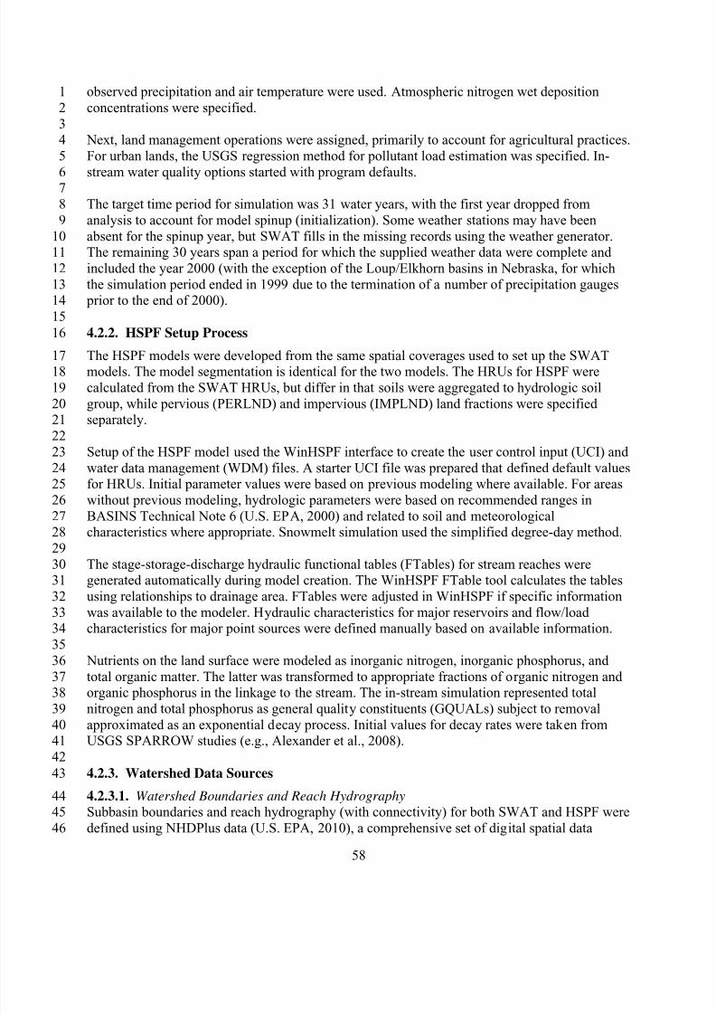
8/13/2019 20 Watersheds Erd
http://slidepdf.com/reader/full/20-watersheds-erd 70/186
1
2
34
5
67
8
9
1011
12
1314
15
16
1718
19
2021
22
23
2425
26
27
2829
3031
32
3334
35
36
3738
394041
42
43
4445
46
observed precipitation and air temperature were used. Atmospheric nitrogen wet deposition
concentrations were specified.
Next, land management operations were assigned, primarily to account for agricultural practices.
For urban lands, the USGS regression method for pollutant load estimation was specified. In-
stream water quality options started with program defaults.
The target time period for simulation was 31 water years, with the first year dropped from
analysis to account for model spinup (initialization). Some weather stations may have been
absent for the spinup year, but SWAT fills in the missing records using the weather generator.The remaining 30 years span a period for which the supplied weather data were complete and
included the year 2000 (with the exception of the Loup/Elkhorn basins in Nebraska, for which
the simulation period ended in 1999 due to the termination of a number of precipitation gauges prior to the end of 2000).
4.2.2. HSPF Setup Process
The HSPF models were developed from the same spatial coverages used to set up the SWATmodels. The model segmentation is identical for the two models. The HRUs for HSPF were
calculated from the SWAT HRUs, but differ in that soils were aggregated to hydrologic soil
group, while pervious (PERLND) and impervious (IMPLND) land fractions were specifiedseparately.
Setup of the HSPF model used the WinHSPF interface to create the user control input (UCI) and
water data management (WDM) files. A starter UCI file was prepared that defined default valuesfor HRUs. Initial parameter values were based on previous modeling where available. For areas
without previous modeling, hydrologic parameters were based on recommended ranges in
BASINS Technical Note 6 (U.S. EPA, 2000) and related to soil and meteorological
characteristics where appropriate. Snowmelt simulation used the simplified degree-day method.
The stage-storage-discharge hydraulic functional tables (FTables) for stream reaches weregenerated automatically during model creation. The WinHSPF FTable tool calculates the tables
using relationships to drainage area. FTables were adjusted in WinHSPF if specific information
was available to the modeler. Hydraulic characteristics for major reservoirs and flow/loadcharacteristics for major point sources were defined manually based on available information.
Nutrients on the land surface were modeled as inorganic nitrogen, inorganic phosphorus, and
total organic matter. The latter was transformed to appropriate fractions of organic nitrogen andorganic phosphorus in the linkage to the stream. The in-stream simulation represented total
nitrogen and total phosphorus as general quality constituents (GQUALs) subject to removalapproximated as an exponential decay process. Initial values for decay rates were taken fromUSGS SPARROW studies (e.g., Alexander et al., 2008).
4.2.3. Watershed Data Sources
4.2.3.1. Watershed Boundaries and Reach Hydrography
Subbasin boundaries and reach hydrography (with connectivity) for both SWAT and HSPF were
defined using NHDPlus data (U.S. EPA, 2010), a comprehensive set of digital spatial data
58
8/13/2019 20 Watersheds Erd
http://slidepdf.com/reader/full/20-watersheds-erd 71/186
1
2
34
5
67
8
9
1011
12
1314
15
16
1718
19
2021
22
2324
25
2627
28
2930
31
32
3334
35
3637
38
3940
41
42
4344
45
representing the surface water of the U.S. including lakes, ponds, streams, rivers, canals, and
oceans. NHDPlus provided catchment/reach flow connectivity, allowing for creation of large
model subbasins with automation. NHDPlus incorporates the National Hydrography Dataset(NHD), the National Elevation Dataset (NED), the National Land Cover Dataset (NLCD), and
the Watershed Boundary Dataset (WBD). A MapWindow script was developed to automate
(with supervision) the aggregation of NHDPlus catchments/reaches into model subbasins andreaches. The general approach was to first run the aggregation script with a smaller target
subbasin size (i.e., create several hundred to a thousand subbasins), then run the script again to
create watersheds of the target model size (comparable to the HUC10 scale). The two tiered
approach has several benefits; it was found to be more time efficient, it allowed for greatercontrol over the final basin size, and it provided a midpoint that could be used to redefine
subbasin boundaries to match specified locations, such as gaging stations and dams/diversions.
Each delineated subbasin was conceptually represented with a single stream assumed to be a
completely mixed, one-dimensional segment with a constant cross-section. For the HSPF model,
reach slopes were calculated based on Digital Elevation Model (DEM) data and stream lengths
were measured from the original NHD stream coverage. Assuming representative trapezoidalgeometry for all streams, mean stream depth and channel width were estimated using regression
curves that relate upstream drainage area to stream dimensions developed for three regions in the
Eastern United States. Existing and more detailed models provided additional site-specificinformation on channel characteristics for some watersheds (e.g., Minnesota River; Tetra Tech,
2008b).
The SWAT model also automatically calculates the initial stream geometric values based on
subbasin drainage areas, standard channel forms, and elevation, using relationships developed for
numerous areas of the United States. Channel slope is automatically calculated from the DEM.
4.2.3.2. Elevation
Topography was represented by digital elevation models (DEMs) with a resolution of 30 metersobtained from USGS’ National Elevation Dataset (Gesch et al., 2002). Multiple DEM coverages
were grouped and clipped to the extent of the model watershed area (with a 10-mile buffer to
allow for unforeseen changes to watershed boundaries).
4.2.3.3. Land Use and Land Cover
The SWAT and HSPF models use a common land use platform representing current (calibration)
conditions and derived from the 2001 National Land Cover Database or NLCD (Homer et al.,2004; Homer et al., 2007). The 2001 NLCD land cover was used to ensure consistency between
all models for the project. The 2001 land use was chosen rather than the 2006 coverage because
it is closer in time to the calibration period of the models, which typically runs through 2002/3.The 2001 land use is assumed to apply throughout the baseline model application period.
Some additional processing of the NLCD data was necessary. Several of the land use classes
were aggregated into more general categories to provide a more manageable set of HRUs. Thedeveloped land classes were kept separate for SWAT but aggregated for HSPF. This is because
SWAT assigns percent imperviousness to total developed area, whereas HSPF explicitly
59
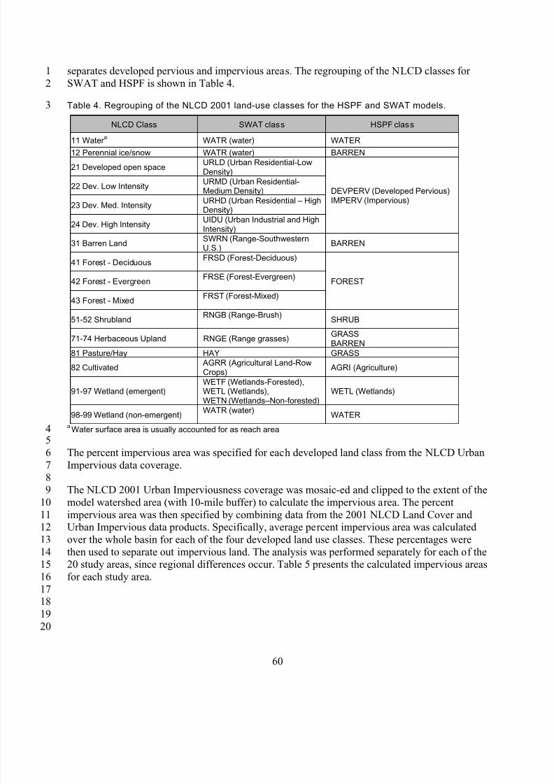
8/13/2019 20 Watersheds Erd
http://slidepdf.com/reader/full/20-watersheds-erd 72/186
1
2
3
45
6
7
89
10
1112
13
1415
16
1718
19
20
separates developed pervious and impervious areas. The regrouping of the NLCD classes for
SWAT and HSPF is shown in Table 4.
Table 4. Regrouping of the NLCD 2001 land-use classes for the HSPF and SWAT models.
NLCD Class SWAT class HSPF class
11 Water a WATR (water) WATER
12 Perennial ice/snow WATR (water) BARREN
21 Developed open spaceURLD (Urban Residential-LowDensity)
DEVPERV (Developed Pervious)IMPERV (Impervious)
22 Dev. Low IntensityURMD (Urban Residential-Medium Density)
23 Dev. Med. IntensityURHD (Urban Residential – HighDensity)
24 Dev. High IntensityUIDU (Urban Industrial and HighIntensity)
31 Barren LandSWRN (Range-SouthwesternU.S.)
BARREN
41 Forest - DeciduousFRSD (Forest-Deciduous)
FOREST42 Forest - Evergreen FRSE (Forest-Evergreen)
43 Forest - MixedFRST (Forest-Mixed)
51-52 ShrublandRNGB (Range-Brush)
SHRUB
71-74 Herbaceous Upland RNGE (Range grasses)GRASSBARREN
81 Pasture/Hay HAY GRASS
82 Cultivated AGRR (Agricultural Land-RowCrops)
AGRI (Agriculture)
91-97 Wetland (emergent)WETF (Wetlands-Forested),WETL (Wetlands),WETN (Wetlands–Non-forested)
WETL (Wetlands)
98-99 Wetland (non-emergent) WATR (water) WATER
aWater surface area is usually accounted for as reach area
The percent impervious area was specified for each developed land class from the NLCD Urban
Impervious data coverage.
The NLCD 2001 Urban Imperviousness coverage was mosaic-ed and clipped to the extent of the
model watershed area (with 10-mile buffer) to calculate the impervious area. The percent
impervious area was then specified by combining data from the 2001 NLCD Land Cover andUrban Impervious data products. Specifically, average percent impervious area was calculated
over the whole basin for each of the four developed land use classes. These percentages were
then used to separate out impervious land. The analysis was performed separately for each of the20 study areas, since regional differences occur. Table 5 presents the calculated impervious areas
for each study area.
60
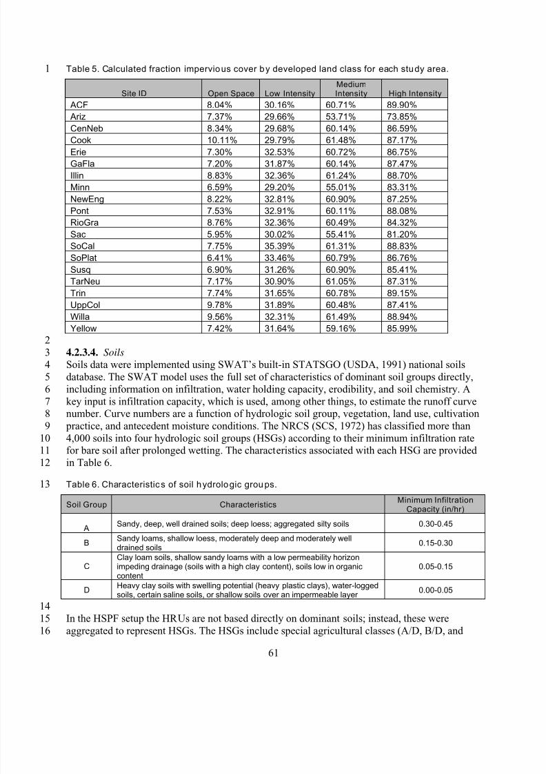
8/13/2019 20 Watersheds Erd
http://slidepdf.com/reader/full/20-watersheds-erd 73/186
1 Table 5. Calculated fraction impervious cover by developed land class for each study area.
Site ID Open Space Low IntensityMediumIntensity High Intensity
ACF 8.04% 30.16% 60.71% 89.90%
Ariz 7.37% 29.66% 53.71% 73.85%
CenNeb 8.34% 29.68% 60.14% 86.59%
Cook 10.11% 29.79% 61.48% 87.17%
Erie 7.30% 32.53% 60.72% 86.75%
GaFla 7.20% 31.87% 60.14% 87.47%
Illin 8.83% 32.36% 61.24% 88.70%
Minn 6.59% 29.20% 55.01% 83.31%
NewEng 8.22% 32.81% 60.90% 87.25%
Pont 7.53% 32.91% 60.11% 88.08%
RioGra 8.76% 32.36% 60.49% 84.32%
Sac 5.95% 30.02% 55.41% 81.20%
SoCal 7.75% 35.39% 61.31% 88.83%
SoPlat 6.41% 33.46% 60.79% 86.76%
Susq 6.90% 31.26% 60.90% 85.41%TarNeu 7.17% 30.90% 61.05% 87.31%
Trin 7.74% 31.65% 60.78% 89.15%
UppCol 9.78% 31.89% 60.48% 87.41%
Willa 9.56% 32.31% 61.49% 88.94%
Yellow 7.42% 31.64% 59.16% 85.99%
2
34
5
6
78
9
1011
12
13
4.2.3.4. Soils
Soils data were implemented using SWAT’s built-in STATSGO (USDA, 1991) national soils
database. The SWAT model uses the full set of characteristics of dominant soil groups directly,
including information on infiltration, water holding capacity, erodibility, and soil chemistry. A
key input is infiltration capacity, which is used, among other things, to estimate the runoff curvenumber. Curve numbers are a function of hydrologic soil group, vegetation, land use, cultivation
practice, and antecedent moisture conditions. The NRCS (SCS, 1972) has classified more than
4,000 soils into four hydrologic soil groups (HSGs) according to their minimum infiltration ratefor bare soil after prolonged wetting. The characteristics associated with each HSG are provided
in Table 6.
Table 6. Characteristic s of soil hydrologic groups.
C
Soil Group
A
B
D
Clay loam soils, shallow sandy loams with a low permeability horizonimpeding drainage (soils with a high clay content), soils low in organiccontent
Characteristics
Sandy, deep, well drained soils; deep loess; aggregated silty soils
Sandy loams, shallow loess, moderately deep and moderately welldrained soils
Heavy clay soils with swelling potential (heavy plastic clays), water-loggedsoils, certain saline soils, or shallow soils over an impermeable layer
0.05-0.15
Minimum InfiltrationCapacity (in/hr)
0.30-0.45
0.15-0.30
0.00-0.05
14
15
16
In the HSPF setup the HRUs are not based directly on dominant soils; instead, these were
aggregated to represent HSGs. The HSGs include special agricultural classes (A/D, B/D, and
61
8/13/2019 20 Watersheds Erd
http://slidepdf.com/reader/full/20-watersheds-erd 74/186
1
2
34
5
67
8
9
1011
12
1314
15
16
1718
19
2021
22
2324
25
2627
28
2930
31
32
3334
35
3637
38
3940
41
42
4344
45
46
C/D) in which the first letter represents conditions with artificial drainage and the second letter
represents conditions without drainage. The first designator was assumed to apply to all crop
land, while the second designator was assumed for all other land uses.
4.2.3.5. Point Source Discharges
The primary objective of this study is to examine relative changes that are potentially associatedwith changes in climate and land use. From that perspective, point source discharges can be
characterized as a nuisance parameter. However, point sources that are large enough relative to
native flows to affect the observed flows and nutrient loads in river systems need to be included
to calibrate the models. This is done in a simplified way, and the point sources were then heldconstant for future conditions, allowing analysis of relative change. Only the major dischargers,
typically those with a discharge rate greater than 1 million gallons per day (MGD) were included
in the models. The major dischargers account for the majority of the total flow from all permitteddischarges in most watersheds, so the effect on the calibration of omitting smaller sources is
relatively small, except perhaps during extreme low flow conditions. Data were sought from the
EPA’s Permit Compliance System (PCS) database for the major dischargers in the watersheds.
Facilities that were missing TN, TP, or TSS concentrations were filled with a typical pollutantconcentration value from literature based on Standard Industrial Classification (SIC) code. The
major dischargers were represented at long-term average flows, without accounting for changes
over time or seasonal variations.
4.2.3.6. Atmospheric Deposition
Atmospheric deposition can be a significant source of inorganic nitrogen to watersheds andwaterbodies. SWAT2005 allows the user to specify wet atmospheric deposition of nitrate
nitrogen. This is specified as a constant concentration across the entire watershed. Wet
deposition of ammonia and dry deposition of nitrogen is not addressed in the SWAT2005 model.
HSPF allows the specification of both wet and dry deposition of both nitrate nitrogen and
ammonia nitrogen and both were included in the model. Dry deposition is specified as a loadingseries, rather than concentration series. Because wet deposition is specified as a concentration it
will vary in accordance with precipitation changes in future climate scenarios, whereas the dry
deposition series (HSPF only) is assumed constant for future scenarios.
Total oxidized nitrogen (NOx) emissions in the U.S. remained relatively constant to a first
approximation across the model period considered in this study from the early 1970s up through
2002 (U.S. EPA, 2002). There is strong geographic variability in atmospheric deposition, butmuch smaller year to year variability at the national scale over this period (Suddick and
Davidson, 2012). The National Acid Deposition Program (NADP; http://nadp.sws.uiuc.edu/)
monitors wet deposition across the country and produces yearly gridded maps of NO3 and NH4
wet deposition concentrations. Dry deposition rates are monitored (and interpreted with models)
by the EPA Clean Air Status and Trends Network (CASTNET;
http://epa.gov/castnet/javaweb/index.html). Results for year 2000 were selected as generally
representative and each study watershed was characterized by a spatial average wet depositionconcentration (and dry deposition loading rate for HSPF). Atmospheric deposition of phosphorus
and sediment was not considered a significant potential source and is not addressed in the
models.
62
8/13/2019 20 Watersheds Erd
http://slidepdf.com/reader/full/20-watersheds-erd 75/186
1
2
34
5
67
8
9
1011
12
1314
15
16
1718
19
2021
22
2324
25
2627
28
2930
31
32
3334
35
3637
38
3940
41
42
4344
4.2.3.7. Impoundments, Diversions, and Withdrawals
The hydrology of many large watersheds in the United States is strongly impacted byanthropogenic modifications, including large impoundments and withdrawals for consumptive
use. It is necessary to take these factors into account to develop a calibrated model. At the same
time, these anthropogenic factors constitute a problem for evaluating response to future changes,as there is no clear basis for evaluating future changes in reservoir operations or water
withdrawals. In addition, information on impoundments, withdrawals, and trans-basin water
imports is often difficult to obtain. The approach taken in this project is to minimize the
importance of impoundments and withdrawals by focusing on relative changes between presentand future conditions with these factors held constant. In this way, the results that are presented
are estimates of the change that may be anticipated based on changes to meteorological and land
use forcing within the subject study area, with other factors held constant. The results providedhere are not complete estimates of future hydrology and pollutant conditions because the
adaptive response of human society to water resources management is not included.
The general approach adopted for this project was to select study areas avoiding major humaninterventions (e.g., reservoirs) in the flow system where possible, to ignore relatively minor
interventions, and where necessary to represent significant interventions in a simplified manner.
In the first instance, study watersheds were delineated to avoid major reservoirs where possible.For example, the model of the Verde River watershed in the Central Arizona basins is terminated
at the inflow to Horseshoe Reservoir. In some cases, as in the Sacramento River watershed, an
upstream reservoir is treated as a constant boundary condition because information on futurereservoir management responses to climate change was not available.
Impoundments, withdrawals, and water imports that do not have a major impact on downstreamflows were generally omitted from the large scale models. Inclusion or omission of such features
was a subjective choice of individual modelers; however, it was generally necessary to include
such features if they resulted in a modification of flow at downstream gages on the order of 10 percent or more. Where these features were included they were represented in a simplified
manner: (1) impoundments were represented by simplified (two-season) stage-discharge
operating rules, developed either from documented operational procedures or from analysis of
monitored discharge; (2) large withdrawals were represented as either annual or monthlyconstant average rates; and (3) major trans-basin water imports were also represented as either
annual or monthly constant average rates depending on availability of data. Use of surface water
for irrigation was simulated only in those basins where it was determined during calibration thatit was a significant factor in the overall water balance. These simplifying assumptions decrease
the quality of model fit during calibration and validation, but provide a stable basis for the
analysis of relative response to climate and land use change within the basin.
The impoundments and other anthropogenic influences on hydrology included in each watershed
model are presented in the Assumptions sections of each of the individual calibration reports for
the 20 study watersheds (see Appendices D through W).
63
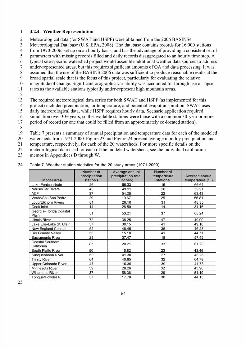
8/13/2019 20 Watersheds Erd
http://slidepdf.com/reader/full/20-watersheds-erd 76/186
1 4.2.4. Weather Representation
Meteorological data (for SWAT and HSPF) were obtained from the 2006 BASINS4
Meteorological Database (U.S. EPA, 2008). The database contains records for 16,000 stations
from 1970-2006, set up on an hourly basis, and has the advantage of providing a consistent set of parameters with missing records filled and daily records disaggregated to an hourly time step. A
typical site-specific watershed project would assemble additional weather data sources to addressunder-represented areas, but this requires significant amounts of QA and data processing. It wasassumed that the use of the BASINS 2006 data was sufficient to produce reasonable results at the
broad spatial scale that is the focus of this project, particularly for evaluating the relative
magnitude of change. Significant orographic variability was accounted for through use of lapserates as the available stations typically under-represent high mountain areas.
The required meteorological data series for both SWAT and HSPF (as implemented for this
project) included precipitation, air temperature, and potential evapotranspiration. SWAT usesdaily meteorological data, while HSPF requires hourly data. Scenario application required
simulation over 30+ years, so the available stations were those with a common 30-year or more
period of record (or one that could be filled from an approximately co-located station).
Table 7 presents a summary of annual precipitation and temperature data for each of the modeled
watersheds from 1971-2000. Figure 23 and Figure 24 present average monthly precipitation andtemperature, respectively, for each of the 20 watersheds. For more specific details on the
meteorological data used for each of the modeled watersheds, see the individual calibration
memos in Appendices D through W.
Table 7. Weather station statistics for the 20 study areas (1971-2000).
2
3
45
678
9
1011
12
13
1415
16
1718
19
2021
22
23
24
Number of Average annual Number ofprecipitation precipitation total temperature Average annual
Model Area stations (inches) stations temperature (°F)
Lake Pontchartrain 26 66.33 15 66.64
Neuse/Tar Rivers 40 49.91 28 59.91
ACF 37 54.26 22 63.43
Verde/Salt/San Pedro 29 19.67 25 56.81
Loup/Elkhorn Rivers 81 26.10 31 48.35
Cook Inlet 14 28.50 14 34.16
Georgia-Florida CoastalPlain
51 53.21 37 68.24
Illinois River 72 38.25 47 49.00
Lake Erie-Lake St. Clair 57 38.15 41 49.10
New England Coastal 52 48.45 36 46.23
Rio Grande Valley 53 15.18 41 44.71
Sacramento River 28 37.47 18 57.45
Coastal SouthernCalifornia 85 20.21 33 61.20
South Platte River 50 16.82 23 43.46
Susquehanna River 60 41.30 27 48.26
Trinity River 64 40.65 32 64.78
Upper Colorado River 47 16.36 39 41.73
Minnesota River 39 28.26 32 43.90
Willamette River 37 58.38 29 51.19
Tongue/Powder R. 37 17.70 30 44.15
25
64
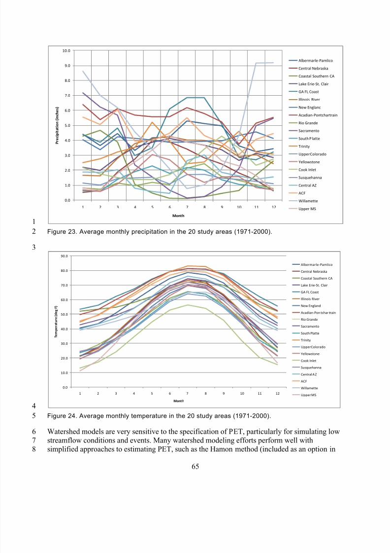
8/13/2019 20 Watersheds Erd
http://slidepdf.com/reader/full/20-watersheds-erd 77/186
0.0
1.0
2.0
3.0
4.0
5.0
6.0
7.0
8.0
9.0
10.0
1 2 3 4 5 6 7 8 9 10 11 12
P r e c i p i t a t i o n ( i n c h e s )
Mont h
Albermarle-Pamlico
Central Nebraska
Coastal Southern CA
Lake Erie-St. Clair
GA FL Coast
Illinois River
New England
Acadian-Pontchartrain
Rio Grande
Sac ramento
South P latte
Trinity
Upper Colorado
Yellowstone
Cook Inlet
Susquehanna
Central AZ
ACF
Willamette
Upper MS
1
2
3
4
5
6
7
8
Figure 23. Average monthly precipitation in the 20 study areas (1971-2000).
0.0
10.0
20.0
30.0
40.0
50.0
60.0
70.0
80.0
90.0
1 2 3 4 5 6 7 8 9 10 11 12
T e m p e r a t u r e ( d e g F )
Mont h
Albermarle-Pamlico
Central Nebraska
Coastal Southern CA
Lake Erie-St. Clair
GA FL Coast
Illinois River
New England
Acadian-Pon tchar train
Rio Grande
Sacramento
South Platte
Trinity
Upper Colorado
Yellowstone
Cook Inlet
Susquehanna
Central A Z
ACF
Willamette
Upper MS
Figure 24. Average monthly temperature in the 20 study areas (1971-2000). Watershed models are very sensitive to the specification of PET, particularly for simulating low
streamflow conditions and events. Many watershed modeling efforts perform well with
simplified approaches to estimating PET, such as the Hamon method (included as an option in
65
8/13/2019 20 Watersheds Erd
http://slidepdf.com/reader/full/20-watersheds-erd 78/186
1
2
34
5
67
8
9
1011
12
1314
15
16
1718
19
2021
22
23
2425
26
27
2829
3031
32
3334
35
36
3738
3940
4142
43
44
4546
the BASINS dataset), which depend primarily on air temperature. However, the robustness of
watershed model calibrations conducted with simplified PET is suspect under conditions of
climate change, since a variety of other factors that influence PET, such as wind speed and cloudcover, are also likely to change. Therefore, we implemented the Penman-Monteith PET, which
employs a full energy balance (Monteith, 1965; Jensen et al., 1990). The implementation varies
slightly between SWAT and HSPF: In SWAT the full Penman-Monteith method (Allen et al.,2005) is implemented as an internal option in the model, and includes feedback from crop height.
For HSPF, Penman-Monteith reference evapotranspiration at each weather station was calculated
externally using observed precipitation and temperature coupled with SWAT weather generator
estimates of solar radiation, wind movement, cloud cover, and relative humidity. An evaluationof the parameters used to calculate potential evapotranspiration indicated gaps (especially for
solar radiation and cloud cover); hence the SWAT weather generator was used to estimate these
parameters. HSPF does not simulate crop growth, so monthly coefficients are incorporated in themodel to convert reference crop PET to values appropriate to different crop stages using the
Food and Agriculture Organization (FAO) method (Allen et al., 1998).
4.3. MODEL SIMULATION ENDPOINTSClimate and land use change both have the potential to introduce significant changes in the
hydrologic cycle. At the larger scale, flow volumes and the seasonal timing of flow are of
immediate and obvious concern. Flows are analyzed in a variety of ways over the 30-yearanalysis period, including the minimum, median, mean, and maximum change relative to
existing conditions among the different scenarios. Because of biases inherent in modeling at this
scale, estimates of relative change between historical and future simulations are most relevant. In
addition to basic flow statistics, comparisons are made for 100-year flood peak (fit with LogPearson type III distribution; USGS, 1982), average annual 7-day low flow, Richards-Baker
flashiness index (a measure of the frequency and rapidity of short term changes in streamflow;
Baker et al., 2004), and days to the centroid of mass for the annual flow on a water-year basis
(i.e., days from previous October 1 at which half of the flow for the water year is achieved, animportant indicator of changes in the snow accumulation and melt cycle). For the Log Pearson
III estimator, use of a regionalized skew coefficient is not appropriate to climate change scenarioapplications as the regional map represents existing climate. Therefore, the K factor is estimated
using the skew coefficient from the model output only, without any weighting with the regional
estimate.
Each of the flow metrics discussed in the preceding section has been evaluated for each scenario
at the output of each HUC8 contained within a study area. Several other summary measures of
the water balance, largely drawn from the work of Hurd et al. (1999), are summarized asaverages at the whole-watershed scale. These are:
• Dryness Ratio, defined here as the fraction of precipitation that is lost toevapotranspiration (ET) as reported by the SWAT model. Hurd et al. calculated a
dryness ratio by computing ET as the difference between precipitation and basin outflow.Results are generally similar, but the latter approach does not account for additional
factors such as channel loss and is affected by reservoir management and boundary
conditions.
• Low Flow Sensitivity, expressed as the rate of baseflow generation by shallowgroundwater, tile drainage, and lateral subsurface flow pathways in units of cfs/mi .
2
66
8/13/2019 20 Watersheds Erd
http://slidepdf.com/reader/full/20-watersheds-erd 79/186
12
34
5
67
89
10
11
1213
14
1516
171819
20
2122
23
24
2526
27
2829
30
31
32
33
34
35
3637
38
3940
41
42
• Surface Runoff Fraction - the fraction of total flow from the uplands that is predicted to proceed through overland flow pathways.
• Snowmelt Fraction – the fraction of total flow from the uplands that is generated bymelting snow.
• Deep Recharge Rate – the annual average depth of water simulated as recharging deep
aquifers.
Table 8 provides a summary of streamflow and water quality endpoints evaluated in this study.
The mobilization and transport of pollutants will also be affected by climate and land use change,
both as a direct result of hydrologic changes and through changes in land cover and plant growth.
Monthly and annual loads of sediment, phosphorus, and nitrogen are likely the most useful andreliable measures of water quality produced by the analysis. Accordingly, the focus of
comparison among scenarios is on monthly and average annual loads for TSS, total nitrogen, and
total phosphorus. As with the flow simulation, it is most appropriate to examine relative ratherthan absolute changes in simulated pollutant loads when comparing scenarios to current
conditions. All models are calibrated and validated, but in many cases current loads areimprecisely known due to limited monitoring data.
Because the sediment load in rivers/streams is often dominated by channel adjustment processes,
which are highly site-specific and occur at a fine spatial scale, it is anticipated that precision inthe prediction of sediment and sediment-associated pollutant loads will be relatively low.
Nutrient balances can also be strongly affected by biological processes in the channels, which
can only be roughly approximated at the scale of modeling proposed.
Note that the modeling protocol assumes that several external and anthropogenic factors remain
constant in the change simulations:
• External boundary conditions (if needed), such as upstream inflows and pollutant loads, are
assumed constant.
• Interactions with deep groundwater systems are assumed constant
• Point source discharges and water withdrawals are assumed constant
• No provision is made for human adaptation in rural land management, such as shifts in crop type
in response to climate change
• Plant growth responses to climate change are simulated to the extent they are represented in the
SWAT plant growth model; however, large-scale shifts in natural cover type in response toclimate change are not simulated.
These assumptions, along with the known large uncertainties associated with modeling regional
climate and land use changes several decades into the future, mean that the results that are presented reflect the effects of simulated climate and land use changes on simulated direct
hydrologic and pollutant loading impacts that arise within a study area. They represent the range
of responses consistent with the current state-of-the-art of modeling future climate and land use
67
8/13/2019 20 Watersheds Erd
http://slidepdf.com/reader/full/20-watersheds-erd 80/186
1
2
3
4
conditions, given the assumptions above, as well as additional assumptions such as reliance on
the Intergovernmental Panel on Climate Change (IPCC) A2 emissions scenario, but in no way
should be construed to represent forecasts of future conditions.
Table 8. Summary of streamflow and water quality endpoin ts.
Endpoint Dimension Description CalculationFuture Flow Volume L
3/t Average of simulated flow
volume
Sum of annual flow volume
simulated by the watershed
model
Average Seven Day
Low Flow
L3/t Average annual 7-day low
flow event
Lowest 7-day-average flow
simulated for each year
100 Year Peak Flow L3/t Estimated peak flow based on
annual flow maxima series,
Log Pearson III method
Log Pearson III extreme value
estimate following USGS (1982),
based on simulated annual
maxima series
Days to Flow Centroid t (days) Number of days from the
previous October 1 (start of
water year) at which half of
the flow volume for that
water year is achieved
Count of days to 50% of
simulated total annual flow
volume for each water year.
Richards-Baker
Flashiness Index
dimension-
less
Indicator of the frequency and
rapidity of short term changes
in daily flow rates
Analyzed by method given in
Baker et al., 2004, applied to
daily flow series for each year
Dryness Ratio dimension-
less
Fraction of input precipitation
lost to evapotranspiration (ET)
Calculated as (precipitation –
outflow)/precipitation for
consistency with Hurd et al.
(1999)
Low Flow Sensitivity L/t Rate of baseflow
contributions from shallow
groundwater, tile drainage,
and lateral subsurface flowpathways
Sum of simulated flow from
shallow groundwater, tile
drainage, and lateral subsurface
flow pathways divided by area.
Surface Runoff
Fraction
dimension-
less
Fraction of streamflow
contributed by overland flow
pathways
Surface runoff divided by total
outflow.
Snowmelt Fraction dimension-
less
Fraction of streamflow
contributed by snowmelt
Estimated as water equivalent
of simulated snowfall divided by
total precipitation
Deep Recharge L/t Depth of water recharging
deep aquifers per unit time
Total water volume simulated as
lost to deep recharge divided by
area
AET L/t Actual depth of
evapotranspiration lost to theatmosphere per unit time
Evapotranspiration simulated by
the watershed model
PET L/t Theoretical potential
evapotranspiration assuming
moisture not limiting
Potential evapotranspiration
simulated by the Penman-
Monteith method (Jensen et al.,
1990)
Total Suspended
Sediment (TSS)
mass/t Mass load of suspended
sediment exiting stream reach
per unit time
Sum of simulated mass exiting a
stream reach
68
8/13/2019 20 Watersheds Erd
http://slidepdf.com/reader/full/20-watersheds-erd 81/186
Total Phosphorus (TP) mass/t Mass load of total phosphorus
exiting stream reach per unit
time
Sum of simulated mass exiting a
stream reach
Total Nitrogen (TN) mass/t Mass load of total nitrogen
exiting stream reach per unit
time
Sum of simulated mass exiting a
stream reach
12
3
4
56
7
89
10
1112
13
1415
16
17
1819
20
2122
23
2425
26
27
2829
30
3132
33
34
3536
37
3839
40
4.4. MODEL CALIBRATION AND VALIDATION
Hydrology and water quality calibration and validation were conducted for HSPF and SWAT in
each of the five pilot study areas, and for SWAT in 15 non-pilot study areas. The followingsection provides a brief summary of calibration and validation methods and results. Detailed
description of calibration and validation methods and results are included in Appendices D
through W.
Calibration refers to the adjustment or fine-tuning of modeling parameters to reproduce
observations based on field monitoring data. Calibration is required for parameters that cannot bedeterministically and uniquely evaluated from topographic, climatic, physical, and chemical
characteristics of the watershed and compounds of interest. Validation is performed by
application of the calibrated model to different time periods without further parameteradjustments to test the robustness of the calibrated parameter set. If the model exhibited a
significant degradation in performance in the validation period, the calibration process was
revisited.
The calibration and validation approach for the very large watersheds addressed in this study was
to first focus on a single HUC8 within the larger study area (preferably one for which some
modeling was already available along with a good record of flow gaging and water qualitymonitoring data), then extend the calibration to adjacent areas with modifications as needed to
achieve a reasonable fit at multiple spatial scales. Each HUC8 watershed was generally
subdivided into approximately 8 subbasins, approximating the HUC10 scale.
The base period for model application was approximately 1970 to 2000, with some variation
depending on availability of meteorological data, while the base land use was from 2001 NLCD.
In watersheds with significant land use change, moving back too far from 2001 may not providea firm basis for calibration. Therefore, calibration generally focused on approximately the 1991
2001 time period, although the full 1971-2000 period was used for comparison to future changes.
Validation was typically performed on the period before 1991 and/or data from post-1991 atdifferent locations.
4.4.1. Hydrology
The calibration for both HSPF and SWAT endeavored to achieve the range of error statistics fortotal volume, seasonal flows, and high and low flows recommended by Lumb et al. (1994) and
Donigian (2000) for HSPF applications while also maximizing the Nash-Sutcliffe coefficient of
model fit efficiency. Standardized spreadsheet tools were developed to help ensure consistencyin the calibration and validation process across watersheds as well as to speed processing through
use of automation and to provide a standardized set of statistics and graphical comparisons to
69
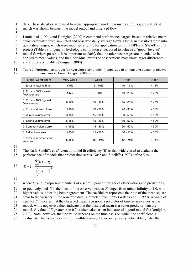
8/13/2019 20 Watersheds Erd
http://slidepdf.com/reader/full/20-watersheds-erd 82/186
1
2
34
5
67
8
9
10
1112
data. These statistics were used to adjust appropriate model parameters until a good statistical
match was shown between the model output and observed flow.
Lumb et al. (1994) and Donigian (2000) recommend performance targets based on relative mean
errors calculated from simulated and observed daily average flows. Donigian classified these into
qualitative ranges, which were modified slightly for application to both HSPF and SWAT in this project (Table 9). In general, hydrologic calibration endeavored to achieve a “good” level of
model fit where possible. It is important to clarify that the tolerance ranges are intended to be
applied to mean values, and that individual events or observations may show larger differences
and still be acceptable (Donigian, 2000).
Table 9. Performance targets fo r hydrologic simu lation (magnitude of annual and seasonal relativemean error). From Donigian (2000).
Model Component Very Good Good Fair Poor
1. Error in total volume ≤5% 5 - 10% 10 - 15% > 15%
2. Error in 50% lowest
flow volumes ≤5% 5 - 10% 10 - 25% > 25%
3. Error in 10% highestflow volumes
≤10% 10 - 15% 15 - 25% > 25%
4. Error in storm volume ≤10% 10 - 20% 20 - 30% > 30%
5. Winter volume error ≤15% 15 - 30% 30 - 50% > 50%
6. Spring volume error ≤15% 15 - 30% 30 - 50% > 50%
7. Summer volume error ≤15% 15 - 30% 30 - 50% > 50%
8. Fall volume error ≤15% 15 - 30% 30 - 50% > 50%
9. Error in summer storm
volumes ≤25% 25 – 50% 50 – 75% > 75%
1314
15
16
17
18
1920
21
22
2324
25
26
The Nash-Sutcliffe coefficient of model fit efficiency ( E ) is also widely used to evaluate the
performance of models that predict time series. Nash and Sutcliffe (1970) define E as:2
∑ n
(O − Pi )i
i=1 , E = 1 − 2
∑ n
(Oi − O) i=1
where Oi and Pi represent members of a set of n paired time series observations and predictions,
respectively, and O is the mean of the observed values. E ranges from minus infinity to 1.0, withhigher values indicating better agreement. The coefficient represents the ratio of the mean square
error to the variance in the observed data, subtracted from unity (Wilcox et al., 1990). A value of zero for E indicates that the observed mean is as good a predictor of time series values as the
model, while negative values indicate that the observed mean is a better predictor than the model. A value of E greater than 0.7 is often taken as an indicator of a good model fit (Donigian,
2000). Note, however, that the value depends on the time basis on which the coefficient is evaluated. That is, values of E for monthly average flows are typically noticeably greater than
70
8/13/2019 20 Watersheds Erd
http://slidepdf.com/reader/full/20-watersheds-erd 83/186
5
10
15
20
25
30
35
40
1
2
34
67
8
9
11
12
1314
16
1718
19
21
22
2324
2627
28
29
31
32
3334
3637
38
39
41
42
values of E for daily flows, as watershed models, in the face of uncertainty in the
representativeness of precipitation records, are often better predictors of inter-seasonal trends
than of intra-seasonal variability. Moriasi et al., (2007) recommend a Nash Sutcliffe E of 0.50 or better (applied to monthly sums) as an indicator of adequate hydrologic calibration when
accompanied by a relative error of 25 percent or less.
A potential problem with the use of E is that it depends on squared differences, making it overly
sensitive to extreme values (Legates and McCabe, 1999). This is particularly problematic for
sparse time series, such as water quality observations, in which poor estimation of one or a few
high outliers may strongly influence the resulting statistic. It is an even greater problem for thecomparison of model output to load estimates based on sparse concentration data, as these
estimates are themselves highly uncertain (using point-in-time grab samples to represent daily
averages and interpolating to unobserved days), further increasing the leverage associated withhigh outliers.
To address these issues and lessen the effect of outliers, Garrick et al. (1978) proposed use of a
baseline adjusted coefficient of model fit efficiency, E 1’, which depends on absolute differencesrather than squared differences:
n
∑ −i
PO ||=−= n
i E 11 1'
∑ −i
OO |'|=i 1
Garrick’s proposed statistic is actually more general, allowing O ’ to be a baseline value that
may be a function of time or of other variables, rather than simply the mean. E 1’ may be similarto or greater or less than E for a given set of predictions and measurements depending on the
type of outliers that are present.
For most watershed models, E is an appropriate measure for the fit of flow time series in which
complete series of observations are known with reasonable precision. E 1’ is a more appropriate
and stable measure for the comparison of simulated pollutant loads to estimates based on sparse
observed data.
4.4.1.1. Calibration Adjustments
HSPF and SWAT hydrology calibration adjustments were made for a range of sensitive parameters selected to represent key watershed processes affecting runoff (U.S. EPA, 2000;
Neitsch et al., 2005; see Table 10 and Table 11, respectively, for selected key parameters most
frequently adjusted). The adjustment of other parameters and the degree of adjustment to each parameter vary by watershed. Details are provided in the individual calibration reports for each
of the watersheds in Appendices D through W.
71
8/13/2019 20 Watersheds Erd
http://slidepdf.com/reader/full/20-watersheds-erd 84/186
1 Table 10. Key hydrology calibration parameters for HSPF.
Parameter name Definition
INFILT Nominal infiltration rate parameter
AGWRC Groundwater recession rate
LZSN Lower zone nominal soil moisture storage
BASETP ET by riparian vegetation
KMELT Degree-day melt factor
PET factor Potential evapotranspiration
DEEPFR Fraction of groundwater inflow that will enter deep groundwater
LZETP Lower zone E-T parameter
2
3 Table 11. Key hydrology calibration parameters for SWAT. Parameter name Definition
CN Curve numbers – varied systematically by land use
ESCO Soil evaporation compensation factor
SURLAG Surface runoff lag coefficient
ALPHA_BF Baseflow alpha factor
GW_DELAY Groundwater delay time
CANMAX Maximum canopy storage
OV_N, CH_N2, CH_N1Manning’s “n” values for overland flow, main channels, and tributarychannels
Sol_AWC Available water capacity of the soil layer, mm water/mm of soil
Bank storage and recession rates Bank storage and recession rates
Snow parameters SFTMP, SMTMP,SMFMX and SMFMN
Snowfall temperature, snowmelt base temperature, maximum melt rate forsnow during year, and minimum melt rate for snow during year
TIMP Snow pack temperature lag factor
CH_K1 Effective hydraulic conductivity in tributary channel alluvium
4
5
6
7
8
9
1011
12
13
1415
1617
18
19
2021
4.4.2. Water Quality
The models in this study are designed to simulate total suspended solids (TSS), total nitrogen,
and total phosphorus. The first objective of calibration was to reduce the relative absolute
deviation between simulated and estimated loads to below 25 percent if possible. The water
quality calibration focuses on the replication of monthly loads, as specified in the project QAPP(Appendix B). While a close match to individual, instantaneous concentration observations
cannot be expected given the approach taken in the model simulations of water quality, the
calibration also examined the general relationship of observed and predicted concentrations with
the intent of minimizing bias relative to flow regime or time of year. Comparison to monthlyloads presents challenges, as monthly loads are not observed. Instead, monthly loads must be
estimated from scattered concentration grab samples and continuous flow records. As a result,the monthly load calibration is inevitably based on the comparison of two uncertain numbers.
Nonetheless, calibration is able to achieve a reasonable agreement. Further, the load comparisons
were supported by detailed examinations of the relationships of flows to loads and
concentrations and the distribution of concentration prediction errors versus flow, time, andseason, as well as standard time series plots.
72
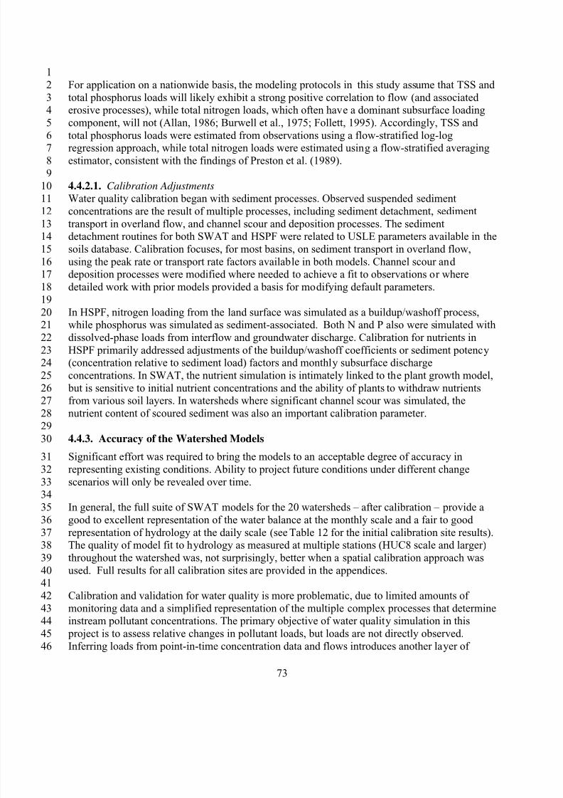
8/13/2019 20 Watersheds Erd
http://slidepdf.com/reader/full/20-watersheds-erd 85/186
1
2
34
5
67
8
9
1011
12
1314
15
16
1718
19
2021
22
2324
25
2627
28
29
30
31
32
3334
35
36
3738
394041
42
4344
45
46
For application on a nationwide basis, the modeling protocols in this study assume that TSS and
total phosphorus loads will likely exhibit a strong positive correlation to flow (and associatederosive processes), while total nitrogen loads, which often have a dominant subsurface loading
component, will not (Allan, 1986; Burwell et al., 1975; Follett, 1995). Accordingly, TSS and
total phosphorus loads were estimated from observations using a flow-stratified log-logregression approach, while total nitrogen loads were estimated using a flow-stratified averaging
estimator, consistent with the findings of Preston et al. (1989).
4.4.2.1. Calibration Adjustments
Water quality calibration began with sediment processes. Observed suspended sediment
concentrations are the result of multiple processes, including sediment detachment, sediment
transport in overland flow, and channel scour and deposition processes. The sedimentdetachment routines for both SWAT and HSPF were related to USLE parameters available in the
soils database. Calibration focuses, for most basins, on sediment transport in overland flow,
using the peak rate or transport rate factors available in both models. Channel scour and
deposition processes were modified where needed to achieve a fit to observations or wheredetailed work with prior models provided a basis for modifying default parameters.
In HSPF, nitrogen loading from the land surface was simulated as a buildup/washoff process,while phosphorus was simulated as sediment-associated. Both N and P also were simulated with
dissolved-phase loads from interflow and groundwater discharge. Calibration for nutrients in
HSPF primarily addressed adjustments of the buildup/washoff coefficients or sediment potency(concentration relative to sediment load) factors and monthly subsurface discharge
concentrations. In SWAT, the nutrient simulation is intimately linked to the plant growth model,
but is sensitive to initial nutrient concentrations and the ability of plants to withdraw nutrientsfrom various soil layers. In watersheds where significant channel scour was simulated, the
nutrient content of scoured sediment was also an important calibration parameter.
4.4.3. Accuracy of the Watershed Models
Significant effort was required to bring the models to an acceptable degree of accuracy in
representing existing conditions. Ability to project future conditions under different change
scenarios will only be revealed over time.
In general, the full suite of SWAT models for the 20 watersheds – after calibration – provide a
good to excellent representation of the water balance at the monthly scale and a fair to good
representation of hydrology at the daily scale (see Table 12 for the initial calibration site results).The quality of model fit to hydrology as measured at multiple stations (HUC8 scale and larger)
throughout the watershed was, not surprisingly, better when a spatial calibration approach wasused. Full results for all calibration sites are provided in the appendices.
Calibration and validation for water quality is more problematic, due to limited amounts of
monitoring data and a simplified representation of the multiple complex processes that determineinstream pollutant concentrations. The primary objective of water quality simulation in this
project is to assess relative changes in pollutant loads, but loads are not directly observed.
Inferring loads from point-in-time concentration data and flows introduces another layer of
73
8/13/2019 20 Watersheds Erd
http://slidepdf.com/reader/full/20-watersheds-erd 86/186
1
2
34
5
67
8
9
1011
12
1314
15
16
1718
19
2021
22
2324
25
2627
28
2930
31
32
uncertainty into the calibration process. Calibration also examined observed versus predicted
concentrations; however, SWAT, as a daily curve number model, does not have a high level of
skill in simulating instantaneous concentrations, particularly during high flow events, and is better suited to the prediction of loads at the weekly to monthly scale.
As with the hydrology calibration, the reliability of the models for simulating changes in waterquality appears to increase with calibration at multiple locations. In general, it is more difficult to
obtain a high level of precision for simulated water quality than for hydrology in a watershed
model, as the processes are complex, the data typically sparse, and any errors in hydrology tend
to be amplified in the water quality simulation. The water quality calibration is based on loads, but loads are not directly observed. Instead, loads are inferred from sparse concentration
monitoring data and flow gaging. Thus, both the simulated and “observed” loads are subject to
considerable uncertainty. Comparison based on concentrations can also be problematic, as mostwater quality samples are grab samples that represent points in time and space, whereas model
output is integrated over a stream segment and may produce large apparent errors due to small
shifts in timing. Finally, most stations at the HUC8 scale include upstream point sources, which
often have a strong influence on low-flow concentrations and load estimates. Limitedknowledge about point source loads thus also creates a challenge for the water quality
calibration. In most cases, the pollutant load simulations from the SWAT model appear to be in
the fair to good range (Table 12) – except in a few cases where parameters were extended fromone station to another watershed without adjustment giving poor results. This suggests limits to
the reliability of simulation results in the portions of watersheds for which calibration was not
pursued. Nonetheless, predictions of relative response to climate and land use change scenariosare likely to be more reliable than quantitative predictions of observed concentrations – as long
as the significant processes that determine pollutant load and transport within a watershed are
represented.
For the pilot sites, HSPF model calibration provided a somewhat stronger fit to daily flows in
four of the five watersheds (Table 13), presumably at least in part due to HSPF’s use of sub-daily precipitation. In two models, the fit to sediment load was notably worse for HSPF, apparently
due to the difficulties in adjusting the more complex channel scour and deposition routines of
this model with limited data and on a compressed schedule.
74
8/13/2019 20 Watersheds Erd
http://slidepdf.com/reader/full/20-watersheds-erd 87/186
Table 12. Summary of SWAT model fit for initial calib ration sit e (20 Watersheds).
Study Area InitialCalibration/ValidationWatershed
InitialCalibration/Validation
USGS Gage
HydrologyCal. /Val.
Years
TotalVolumeCal./Val.(Daily E)
TotalVolumeCal./Val.(% Error)
WaterQualityCal./ValYears
TSS LoadCal./Val.(% Error)
TP LoadCal./Val.(% Error)
TN LoadCal./Val.(% Error)
Apalachicola-Chattahoochee-Flint Upper Flint River 02349605
1993-2002/1983-1992 0.62/0.56 7.28/3.33
1999-2002/1991-1998 -9/17 -50/-30 -18/9
Coastal SouthernCalifornia Basins Santa Ana River 11066460
1991-2001/1981-1991 0.63/0.59 3.71/1.61
1998-2000/ND 19/NA -14.7/NA -5.5/NA
Cook Inlet Basin Kenai River 152663001992-2001/1982-1991 0.68/0.55 -18.96/19.49
1985-2001/1972-1984 66.4/64.1 83.2/82.18 57.3/50.4
Georgia-FloridaCoastal Plain
OchlockoneeRiver 02329000
1992-2002/1982-1992 0.71/0.8 4.25/-5.54
1992-2002/1982-1992 9.5/-6.6 -7.4/-5.8 -8/-5
Illinois River Basin Iroquois River 055260001992-2001/1982-1992 0.7/0.67 -16.99/-2.98
1985-2001/1978-1984 38/39 5/-1 56/60
Lake Erie-Lake St.Clair Drainages
Lake Erie-St. ClairBasin 04208000
1990-2000/1980-1990 0.61/0.62 -3.32/-13.38
1990-2000/1980-1990 67.9/69.8 23.9/-12.5 35.8/13.7
Lake PontchartrainDrainage Amite River 07378500
1995-2004/1985-1994 0.79/0.69 -1.61/-0.93
1984 –1994/ ND 9.2/NA 2.4/NA -8.9/NA
Loup/Elkhorn RiverBasin Elkhorn River 06800500
1989-1999/1978-1988 0.42/0.52 -2.59/-8.81
1990-1995/1979-1989 59.6/66.8 24.2/34.9 28.1/18.1
Minnesota River
Basin Cottonwood River 05317000
1992-2002/
1982-1992 0.79/0.74 -5.41/-0.84
1993-200
/1986-1992 9.2/9 9.3/-21.6 -8.9/-1.3
Neuse/Tar RiverBasins Contentnea Creek 02091500
1993-2003/1983-1993 0.68/0.64 -3.98/-1.18
1993-2003/1983-1993 -19.9/9.9 15.9/5.3 -5.6/5.3
New EnglandCoastal Basins Saco River 01066000
1993-2003/1983-1993 0.61/0.76 1.08/0.67
1993-2003/1983-1993 -9/3.2 9.6/-11.5 27.5/26.3
Powder/TongueRiver Basin Tongue River 06306300
1993-2003/1983-1993 0.72/0.7 9.26/-9.95
1993-2003/1982-2002 -21.8/-3.4 8.8/35.1 3.9/31.5
Rio Grande Valley Saguache Creek 082270001993-2003/1983-1993 0.47/0.07 -4.92/32.99
1985-2003/1973-1984 57.3/41 -46.9/-653.98 -28.3/-909.1
Sacramento RiverBasin Sacramento River 11377100
1992-2001/1983-1992 0.75/0.57 10.23/10.06
1997-2001/1973-1996 -2/-55 -8/-33 -135/-156
75
8/13/2019 20 Watersheds Erd
http://slidepdf.com/reader/full/20-watersheds-erd 88/186
-4.76/-12.1 1986-1990 -12/-7 -114/-105 -72/-66
Study Area Initial Initial Hydrology Total Total Water TSS Load TP Load TN LoadCalibration/ Calibration/ Cal. /Val. Volume Volume Quality Cal./Val. Cal./Val. Cal./Val.Validation Validation Years Cal./Val. Cal./Val. Cal./Val (% Error) (% Error) (% Error)Watershed USGS Gage (Daily E) (% Error ) Years
Salt, Verde, andSan Pedro River 1992-2002/ 1993-2002/Basins Verde River 09504000 1982-1992 0.03/-1 -2.46/5.68 1986-1992 16.9/-42.6 83.5/31.4 -14.4/-15.9
South Platte River 1991-2000/ 1993-2000/Basin South Platte River 06714000 1981-1990 0.74/0.52 9.82/-16.28 ND 86.6/ -14/NA 6.1/NA
Raystown BranchSusquehanna River of the Juniata 1995-2005/ 1991-2000/Basin River 02050303 1985-1995 0.29/0.42 -5.41/16.3 1990 -10.1/-33.6 -0.5/-9.2 28.6/43.9
1992-2001/ 1985-2001/Trinity River Basin Trinity River 05330000 1982-1991 0.62/0.47 -6.88/0.7 1972-1984 9.2/-17.4 3/-21.58 -3.8/-31.9
Upper Colorado 1992-2002/ 1992-2002/River Basin Colorado River 09070500 1982-1992 0.83/0.78 8.18/0.93 1992-1992 0.4/NA 47.4/NA 15.1/NA
Willamette River 1995-2005/ 1991-1995/Basin Tualatin River 14207500 1985-1995 0.49/0.39
Table 13. Summary of HSPF model fit for in itial calibration sites (5 Pilot Watersheds)
Study Area InitialCalibration/ValidationWatershed
Initialcalibration/Validation
USGS Gage
HydrologyCal. /Val.
Years
TotalVolumeCal./Val.(Daily E)
TotalVolumeCal./Val.(% Error)
WaterQualityCal./ValYears
TSS LoadCal./Val.(% Error)
TP LoadCal./Val.(% Error)
TN LoadCal./Val.(% Error)
ApalachicolaChattahoochee-FlintBasins
Upper FlintRiver 02349605
1993-2002/1983-1992 0.707/0.651 5.50/5.79
1999-2002/1991-1998 -117/-78 -59/-23 -30/-22
Minnesota RiverBasin
CottonwoodRiver 05317000
1992-2002/1982-1992 0.754/0.779 1.61/14.78
1993-2002 /1986-1992 7.5/13.1 23/15.8 15.4/16.2
Salt/Verde/SanPedro River Basins Verde River 09504000
1992-2002/1982-1992 0.481/0.451 2.43/6.31
1993-2002 /1986-1992 31/-41 87/66 1.6/-2.7
Susquehanna RiverBasin
RaystownBranch of theJuniata River 02050303
1995-2005/1985-1995 0.698/0.553 -0.16/-8.0
1991-2000 /1990 -78.2/-89.7 26.0/21.5 7.0/17.2
Willamette RiverBasin Tualatin River 14207500
1995-2005/1985-1995 0.731/0.811 -3.92/-9.80
1991-1995/1986-1990 3.0/4.8 -1.2/-9.3 2.2/-6.3
76
8/13/2019 20 Watersheds Erd
http://slidepdf.com/reader/full/20-watersheds-erd 89/186
5
10
15
20
25
30
35
40
1 5. CLIMATE CHANGE AND URBAN DEVELOPMENT SCENARIOS
The SWAT and HSPF models were applied to simulate historical baseline conditions, and
watershed response to future urban development, climate change, and the combined response toclimate change and urban development.
Historical conditions were simulated for each of the 20 watersheds to define baseline, or existing,climate and land use conditions. The base period for model application was 30 years within the
range of 1969-2005, depending on data availability, while the base land use was from the 2001
NLCD, which is also the basis for ICLUS projections. The individual calibration reports inAppendices D through W present the baseline conditions in greater detail.
Climate change scenarios are based on mid-21st century climate model projections downscaled
with regional climate models (RCMs) from the North American Regional Climate ChangeAssessment Program (NARCCAP) and the bias-corrected and spatially downscaled (BCSD) data
set described by Maurer et al. (2007). Fourteen different climate scenarios were applied to the
five pilot watersheds, and a subset of 6 climate scenarios from the NARCCAP archive wereapplied to the non-pilot watersheds. Urban and residential development scenarios are based on
EPA’s national-scale Integrated Climate and Land Use Scenarios (ICLUS) project (U.S. EPA,
2009d). The following sections discuss in more detail climate change and urban developmentscenarios.
5.1. CLIMATE CHANGE SCENARIOS
The scientific uncertainties related to our understanding of the physical climate system are large,and they will continue to be large for the foreseeable future. It is beyond our current capabilities
to predict with accuracy decadal (and longer) climate changes at the regional spatial scales of
relevance for watershed processes (e.g., see Cox and Stephenson, 2007; Stainforth et al., 2007;Raisanen, 2007; Hawkins and Sutton, 2009; among many others). The uncertainties associated
with socioeconomic trajectories, technological advances, and regulatory changes that will drive
greenhouse gas emissions changes (and land use changes) are even larger and less potentially
tractable.
Faced with this uncertainty, an appropriate strategy is to take a scenario-based approach to the
problem of understanding climate change impacts on water quality. A scenario is a plausibledescription of how the future may develop, based on a coherent and internally consistent set of
assumptions about driving forces and key relationships (IPCC, 2007). Scenarios are used in
assessments to provide alternative views of future conditions considered likely to influence a
given system or activity. By systematically exploring the implications of a wide range of plausible alternative futures, or scenarios, we can reveal where the greatest vulnerabilities lie.
This information can be used by decision makers to help understand and guide the development
of response strategies for managing climate risk. A critical step in this approach is to create anumber of plausible future states that span the key uncertainties in the problem. The goal is not
to estimate a single, “most likely” future trajectory for each study watershed, but instead to
understand, to the extent feasible, how big an envelope of potential future impacts we are unableto discount and must therefore incorporate into future planning.
2
34
67
8
9
11
12
1314
1617
18
19
21
22
2324
2627
28
29
31
32
3334
36
3738
39
41
42
4344
77
8/13/2019 20 Watersheds Erd
http://slidepdf.com/reader/full/20-watersheds-erd 90/186
1
2
34
5
67
8
9
1011
12
1314
15
16
1718
19
2021
22
2324
25
2627
28
2930
31
32
3334
35
3637
38
3940
41
42
4344
45
46
Note that, for climate change studies, the word “scenario” is often used in the context of the
Intergovernmental Panel on Climate Change (IPCC) greenhouse gas storylines. The IPCCemissions scenarios describe alternative development pathways, covering a range of
demographic, economic, and technological driving forces that affect GHG emissions. This can
produce some confusion when phrases like “climate change scenarios” are used to refer to thefuture climates simulated using these greenhouse gas storylines. For the purposes of this study,
“scenario” is a generic term that can be applied to any defined future, including a climate future
or a land-use future, among others.
Initial simulation of watershed response to climate change scenarios focused on the five pilot
study basins using both the HSPF and SWAT watershed models. Meteorological datasets
representing a suite of potential climate change scenarios for the period 2041-2070 weredeveloped from the North American Regional Climate Change Assessment Program
(NARCCAP) archive of dynamically downscaled climate products and the BCSD statistically
downscaled output, along with raw (un-downscaled) Global Climate Model (GCM) output
(Table 14). We also explored use of GCMs without downscaling and use of bias-correctedstatistically downscaled (BCSD) scenarios, for a total of 14 climate scenarios. These datasets
were combined with scenarios of future land-use change (residential and urban) acquired from
EPA’s ICLUS project. For the five pilot basins a full range of 14 climate scenarios wereimplemented with both the HSPF and SWAT models with and without future land-use change.
For the remaining 15 non-pilot basins, the 6 available NARCCAP dynamically downscaled
climate products were simulated, with and without land-use change, using the SWAT modelonly.
The general strategy for developing meteorological change scenarios appropriate for input to thewatershed models from the climate change scenarios is to take an approximately 30-year time
series of observed local climate observations (to which the watershed models have been
calibrated) and adjust these observed data to reflect the change in climate as simulated by theglobal and regional climate models (and downscaling approaches). This approach is
implemented for a number of reasons. First, the GCM and RCM output, including the 50-km
NARCCAP scale is still too coarse for watershed modeling. In addition, climate models do not
necessarily archive all the meteorological forcing variables that watershed models expect.Finally, many GCMs display well-documented biases with regard to precipitation frequency and
intensity. Specifically, there is a tendency for GCMs to generate too many low-intensity events
and to under-simulate the intensity of heavy events (Sun et al., 2006; Dai, 2006). The frequencyand duration of large events can have significant effects on hydrology, pollutant loading, and
other watershed processes. Applying the model-derived change statistics to the observed
precipitation time series mitigates this problem.
In practice, when relying on models to develop climate scenarios, this means sampling across
multiple Global Climate Models (GCMs), multiple methodologies for regionalizing or
“downscaling” the model output to finer scales, and, depending on the time horizon considered,multiple greenhouse gas pathways. Use of a single model run is not considered scientifically
rigorous for climate impacts studies. This is because, while the leading GCMs often produce
very different results for future climate change in a given region, there is no consensus in the
78
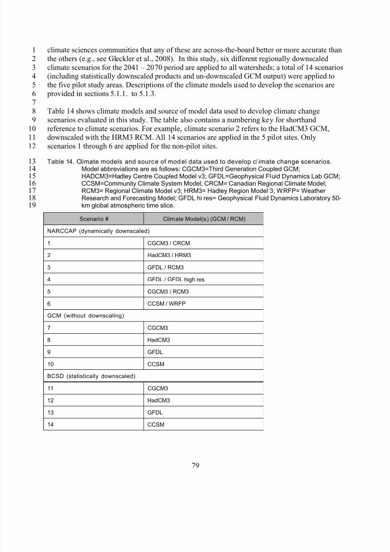
8/13/2019 20 Watersheds Erd
http://slidepdf.com/reader/full/20-watersheds-erd 91/186
1 climate sciences communities that any of these are across-the-board better or more accurate than
the others (e.g., see Gleckler et al., 2008). In this study, six different regionally downscaled
climate scenarios for the 2041 – 2070 period are applied to all watersheds; a total of 14 scenarios(including statistically downscaled products and un-downscaled GCM output) were applied to
the five pilot study areas. Descriptions of the climate models used to develop the scenarios are
provided in sections 5.1.1. to 5.1.3.
Table 14 shows climate models and source of model data used to develop climate change
scenarios evaluated in this study. The table also contains a numbering key for shorthand
reference to climate scenarios. For example, climate scenario 2 refers to the HadCM3 GCM,downscaled with the HRM3 RCM. All 14 scenarios are applied in the 5 pilot sites. Only
scenarios 1 through 6 are applied for the non-pilot sites.
Table 14. Climate models and source of model data used to develop cl imate change scenarios.Model abbreviations are as follows: CGCM3=Third Generation Coupled GCM;HADCM3=Hadley Centre Coupled Model v3; GFDL=Geophysical Fluid Dynamics Lab GCM;CCSM=Community Climate System Model; CRCM= Canadian Regional Climate Model;
RCM3= Regional Climate Model v3; HRM3= Hadley Region Model 3; WRFP= WeatherResearch and Forecasting Model; GFDL hi res= Geophysical Fluid Dynamics Laboratory 50km global atmospheric time slice.
Scenario # Climate Model(s) (GCM / RCM)
NARCCAP (dynamically downscaled)
1 CGCM3 / CRCM
2 HadCM3 / HRM3
3 GFDL / RCM3
4 GFDL / GFDL high res
5 CGCM3 / RCM3
6 CCSM / WRFP
GCM (without downscaling)
7 CGCM3
8 HadCM3
9 GFDL
10 CCSM
BCSD (statistically downscaled)
11 CGCM3
12 HadCM3
13 GFDL
14 CCSM
2
34
5
67
8
9
1011
12
13141516
171819
79
8/13/2019 20 Watersheds Erd
http://slidepdf.com/reader/full/20-watersheds-erd 92/186
1
2
3
4
56
7
89
10
1112
13
1415
16
17
1819
20
2122
23
2425
26
272829
30
31
3233
34
3536
37
3839
40
4142
43
44
45
5.1.1. North American Regional Climate Change Assessment Program (NARCCAP)
Scenarios
Six regionally downscaled climate change scenarios (based on four underlying GCMs) were
acquired from the National Center for Atmospheric Research (NCAR) North American RegionalClimate Change Assessment Program (NARCCAP) project (representative of the future period
2041-2070) (Mearns, 2009; http://www.narccap.ucar.edu). The NARCCAP program uses a
variety of different Regional Climate Models (RCMs) to downscale the output from a few of theIPCC Global Climate Models (GCMs) to higher resolution over the conterminous United States
and most of the rest of North America. NARCCAP’s purpose is to provide detailed scenarios of
regional climate change over the continent, while, by employing the RCMs and GCMs indifferent combinations, systematically investigating the effect of modeling uncertainties on the
scenario results (i.e., uncertainties associated with using different GCMs, RCMs, model physical
parameterizations and configurations). The downscaled output is archived for the periods 19712000 and 2041-2070 at a temporal resolution of three hours.
NARCCAP uses the IPCC’s A2 greenhouse gas storyline. The A2 scenario is a relatively
pessimistic scenario that assumes a very heterogeneous world with high population growth, sloweconomic development, and slow technological change. While no likelihood is attached to any of
the SRES scenarios, emissions are currently rising at rates comparable to those assumed under
the IPCC A2 scenario. Use of a single greenhouse gas storyline is reasonable in this case wherethe focus is on a mid-century future period, as the different IPCC greenhouse gas storylines have
not yet diverged much by this point, and model uncertainty is therefore correspondingly more
important.
5.1.2. Bias-Corrected and Spatially Downscaled (BCSD) Scenarios
At the time modeling was initiated (mid 2010), only six out of a total of 14 planned downscaledscenarios (GCM-RCM combinations) were available from NARCCAP. The dynamicallydownscaled atmospheric models available from NARCCAP are the core climate scenarios for
evaluation of watershed response. However, implementation of RCMs for dynamical
downscaling is a time-consuming and expensive process. A subsidiary research objective for the
five pilot sites was to compare results obtained without full dynamical downscaling. Theseincluded output from the bias-corrected and spatially downscaled (BCSD) methodology (Wood
et al., 2004; Maurer et al., 2007) provided by the World Climate Research Programme’s
(WCRP’s) Coupled Model Intercomparison Project phase 3 (CMIP3) multi-model dataset(Bureau of Reclamation/Santa Clara University/Lawrence Livermore archive of downscaled
IPCC model runs).
The BCSD climate projections derived from CMIP3 data are served at http://go
dcp.ucllnl.org/downscaled_cmip3_projections/. These data use statistical bias correction to
interpret GCMs over a large spatial domain based on current observations. The principal potential weakness of this approach is an assumption of stationarity. That is, the assumption is
made that the relationship between large-scale precipitation and temperature and local
precipitation and temperature in the future will be the same as in the past. Thus, the method can
successfully account for orographic effects that are observed in current data, but not for impacts
80
8/13/2019 20 Watersheds Erd
http://slidepdf.com/reader/full/20-watersheds-erd 93/186
1
2
34
5
67
8
9
1011
12
1314
15
16
1718
19
2021
22
23
24
25
26
27
2829
30
3132
33
3435
36
3738
3940
4142
43
4445
46
that might result from the interaction of changed wind direction and orographic effects. A second
assumption included in the bias-correction step of the BCSD method is that any biases exhibited
by a GCM for the historical period will also be exhibited in simulations of future periods.
The BCSD scenarios, while all derived from the A2 climate storyline, do not in all cases use the
output of the exact same GCM run that was used to construct the NARCCAP archive.Specifically, the BCSD results for the GFDL and CGCM3 GCMs use exactly the same GCM
output as NARCCAP, but BCSD results for HadCM3 and CCSM use different runs of the A2
scenario than used by NARCCAP. The HadCM3 run used in NARCCAP was a custom run
generated specifically for NARCCAP and has not been downscaled for the CMIP3 archive. TheCCSM run used in NARCCAP is run number 5, but this is not available in the CMIP3 archive.
Instead, the BCSD results use the HadCM3 run 1 and CCSM run 4 from the CMIP3 archive for
the A2 scenario. As a result, the most direct comparisons between NARCCAP dynamicdownscaling and BCSD output are for these two models, HadCM3 and CCSM. However, we
still expect comparisons between NARCCAP and BCSD downscaling for the GFDL and
CGCM3 GCMs to provide useful insights when considered along with the HadCM3 and CCSM
comparisons.
5.1.3. Global Climate Models (GCMs) without Downscaling
Scenarios for the five pilot sites also examined use of the direct output from the GCM runs usedto drive the NARCCAP downscaling (i.e., no downscaling). Comparison of results from these
scenarios to full dynamical downscaling is expected to inform the accuracy with which simpler
methods can be used to address watershed response.
5.1.4. Translation of Climate Model Projections to Meteorological Model Inputs
Meteorological time series for input to the watershed models were created using a “change
factor” or “delta change” method. Approximately 30-year time series of observed local climate
observations (to which the watershed models have been calibrated) were adjusted to reflect thechanges in climate as simulated by the climate models. The benefits of this approach include its
simplicity, elimination of the need for bias correction, and ability to create spatially variable
climate change scenarios that maintain the observed historical spatial correlation structure amongdifferent watershed locations. Limitations include the inability to adjust the number and timing
of precipitation events (e.g., to add precipitation events on dry days), and potential bias
introduced through the selection of an arbitrary historical base period that is adjusted.
Change factors for temperature and precipitation were calculated for each month of the year as
the differences between simulated average monthly values for the 2041-2070 and 1971-2000 periods. These change statistics were then used to perturb existing records of hourly observed
precipitation and temperature contained in the BASINS Meteorological Database using theClimate Assessment Tool (CAT) (U.S. EPA, 2009c). CAT permits the sequential modification of
weather records to introduce a number of alterations, each reflecting various assumptionsconcerning the regional manifestations of climate change. Precipitation records can be modified
by (1) multiplying all records by an empirical constant reflecting projected climate change to
simulate a shift in total precipitation, applied uniformly to all periods and intensity classes, (2)selective application of such a multiplier to specific seasons or months, (3) selective application
of the multiplier to a range of months or years within the record, and (4) selective application of
81
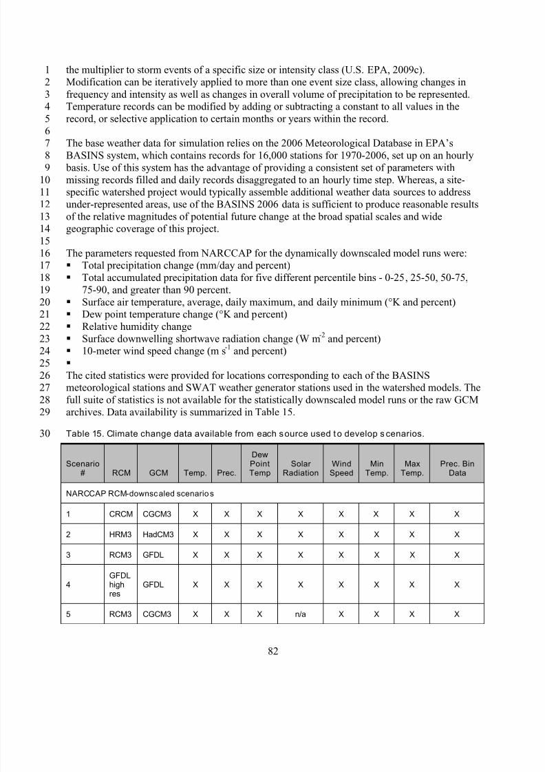
8/13/2019 20 Watersheds Erd
http://slidepdf.com/reader/full/20-watersheds-erd 94/186
1
2
34
5
67
8
9
1011
12
1314
15
16
1718
19
2021
22
2324
25
2627
28
29
30
the multiplier to storm events of a specific size or intensity class (U.S. EPA, 2009c). Modification can be iteratively applied to more than one event size class, allowing changes in frequency and intensity as well as changes in overall volume of precipitation to be represented.Temperature records can be modified by adding or subtracting a constant to all values in the record, or selective application to certain months or years within the record.
The base weather data for simulation relies on the 2006 Meteorological Database in EPA’s BASINS system, which contains records for 16,000 stations for 1970-2006, set up on an hourly basis. Use of this system has the advantage of providing a consistent set of parameters with
missing records filled and daily records disaggregated to an hourly time step. Whereas, a sitespecific watershed project would typically assemble additional weather data sources to address under-represented areas, use of the BASINS 2006 data is sufficient to produce reasonable results of the relative magnitudes of potential future change at the broad spatial scales and widegeographic coverage of this project.
The parameters requested from NARCCAP for the dynamically downscaled model runs were:
Total precipitation change (mm/day and percent)
Total accumulated precipitation data for five different percentile bins - 0-25, 25-50, 50-75,
75-90, and greater than 90 percent. Surface air temperature, average, daily maximum, and daily minimum (°K and percent) Dew point temperature change (°K and percent) Relative humidity change Surface downwelling shortwave radiation change (W m
-2and percent)
10-meter wind speed change (m s-1
and percent)
The cited statistics were provided for locations corresponding to each of the BASINS meteorological stations and SWAT weather generator stations used in the watershed models. The full suite of statistics is not available for the statistically downscaled model runs or the raw GCM archives. Data availability is summarized in Table 15.
Table 15. Climate change data available from each source used to develop s cenarios.
82
Scenario# RCM GCM Temp. Prec.
DewPointTemp
SolarRadiation
WindSpeed
MinTemp.
MaxTemp.
Prec. BinData
NARCCAP RCM-downscaled scenarios
1 CRCM CGCM3 X X X X X X X X
2 HRM3 HadCM3 X X X X X X X X
3 RCM3 GFDL X X X X X X X X
4GFDLhighres
GFDL X X X X X X X X
5 RCM3 CGCM3 X X X n/a X X X X
8/13/2019 20 Watersheds Erd
http://slidepdf.com/reader/full/20-watersheds-erd 95/186
Dew
Scenario Point Solar Wind Min Max Prec. Bin# RCM GCM Temp. Prec. Temp Radiation Speed Temp. Temp. Data
6 WRFP CCSM X X X X
Driving GCMs of the NARCCAP scenarios (i.e., no downscaling)
7 CGCM3 X X X X
8 HadCM3 X X n/a n/a
9 GFDL X X n/a X
10 CCSM X X X X
CMIP3 statistically downscaled scenarios
11 CGCM3 X X n/a n/a
12 HadCM3 X X n/a n/a
13 GFDL X X n/a n/a
14 CCSM X X n/a n/a
X X X X
X n/a n/a n/a
n/a n/a n/a n/a
X n/a n/a n/a
n/a n/a n/a n/a
n/a n/a n/a n/a
n/a n/a n/a n/a
n/a n/a n/a n/a
n/a n/a n/a n/a
1
2 5.1.4.1. Temperature Changes
Implementation of model simulated temperature time series is straightforward. Monthlyvariations (deltas) to the temperature time-series throughout the entire time-period were applied
using the CAT tool. Monthly adjustments based on each scenario were used and a modified
HSPF binary data (WDM) file was created. The temperature time series were adjusted based on
an additive change using the monthly deltas (°K) calculated from the 2041-2070 to 1971-2000climate simulation comparison. Beginning with the HSPF WDM, an automated script then
creates the SWAT observed temperature files (daily maximum and daily minimum).
5.1.4.2. Precipitation Changes
Relative changes in the frequency and intensity of precipitation events associated with climate
change may prove to be more influential in determining future patterns of discharge than changesin overall (annual, seasonal) precipitation. Appendix C presents a summary review of recent
literature to address the following questions: (1) How should precipitation change as a
consequence of lower atmosphere warming? (2) What is the historical evidence for increases in precipitation intensity over the United States? (3) What do climate models simulate with respect
to precipitation frequency and intensity? (4) What are the important limitations in thesesimulations, and (5) What are the implications for the development of meteorological time series
used in the modeling study? In particular, the partitioning of precipitation into re-evaporation,runoff, and percolation to groundwater is understood to be sensitive to the intensity and timing of
precipitation events.
As a general pattern, warming of the lower atmosphere is projected to lead to a more vigorous
hydrologic cycle, characterized by increases in global precipitation, and proportionally larger
34
5
6
78
9
1011
12
1314
15
1617
1819
2021
22
2324
25
83
8/13/2019 20 Watersheds Erd
http://slidepdf.com/reader/full/20-watersheds-erd 96/186
1
2
34
5
67
8
9
1011
12
1314
15
16
1718
19
2021
22
2324
25
2627
28
2930
31
32
3334
35
3637
38
3940
41
42
4344
45
46
increases in high-intensity precipitation events (Trenberth et al., 2007). Much of the U.S. is
anticipated to experience an increasing proportion of annual precipitation as larger, more intense
events (Kundzewicz et al., 2007; Groisman et al., 2005). Increasing intensity of precipitationcould increase direct runoff during events, and increase non-point source loading of sediment,
nutrients, and other pollutants to streams (Gutowski et al., 2008). To ensure that model
simulations embody the most important dimensions of climate change affecting watershedresponse, it is important that climate change scenarios represent potential changes in
precipitation intensity-frequency-duration (IFD) relationships.
In the delta method, future climate time series are constructed by applying changes to observed precipitation time series that represent the relative differences between historical simulations and
future climate scenarios from the climate models. No modifications were made to the number of
rainfall events in the observed record. The most rigorous approach to applying the downscaledclimate scenario results to modification of the existing precipitation series would be to undertake
a detailed analysis (by month) of the distribution of precipitation event volumes and intensities.
Working on an event basis is important because many of the existing precipitation time series in
the BASINS meteorological dataset are disaggregated from daily totals. However, analyzingvolume-event data for each of the climate scenarios for all the precipitation stations was not
feasible and the ability of the climate models to correctly simulate event durations is suspect.
Therefore, a different approach was developed to apply changes in intensity in the precipitationtime series.
Total accumulated precipitation data for different percentile bins (for each station location bymonth) were provided by NARCCAP for the dynamically downscaled climate products. The
data consisted of total simulated precipitation volume (over 30 years) and the 0-25, 25-50, 50-70,
and 70-90, and >90 percentile bins of the 3-hr intensity distribution (relative to the existingintensity distribution). These intensity percentiles yield information on where precipitation
intensification occurs, but represent fixed 3-hr windows, not discrete event volumes, as required
for the CAT tool. Most of the climate scenarios showed increases in precipitation volume in thelarger events, while the smaller ones remained constant or decreased. The net effect of this was
an increase in the proportion of annual precipitation occurring in larger events. Analysis of the
comprehensive (percentile, total volume) climate scenario data showed that, for most weather
stations, the change in the lower percentiles of the intensity distribution appeared to be relativelysmall compared to the changes above the 70
th percentile. However, in some cases (e.g., in
Arizona, there is greater change in the 25-50th
percentile bin).
To account for changes in intensity, climate change scenarios were created using the delta
method by applying climate change adjustments separately to precipitation events ≥ 70th
percentile and events < 70th percentile, while maintaining the appropriate mass balance asdescribed below.
Percentile bin-intensity data were available only for climate scenarios 1 through 6 (RCM
downscaled scenarios). Bin data were not available for climate scenarios 7 through 14 (GCM andstatistically downscaled scenarios). Two approaches were developed to account for
intensification of precipitation, depending on whether precipitation bin data were available. Each
approach is discussed in detail below.
84
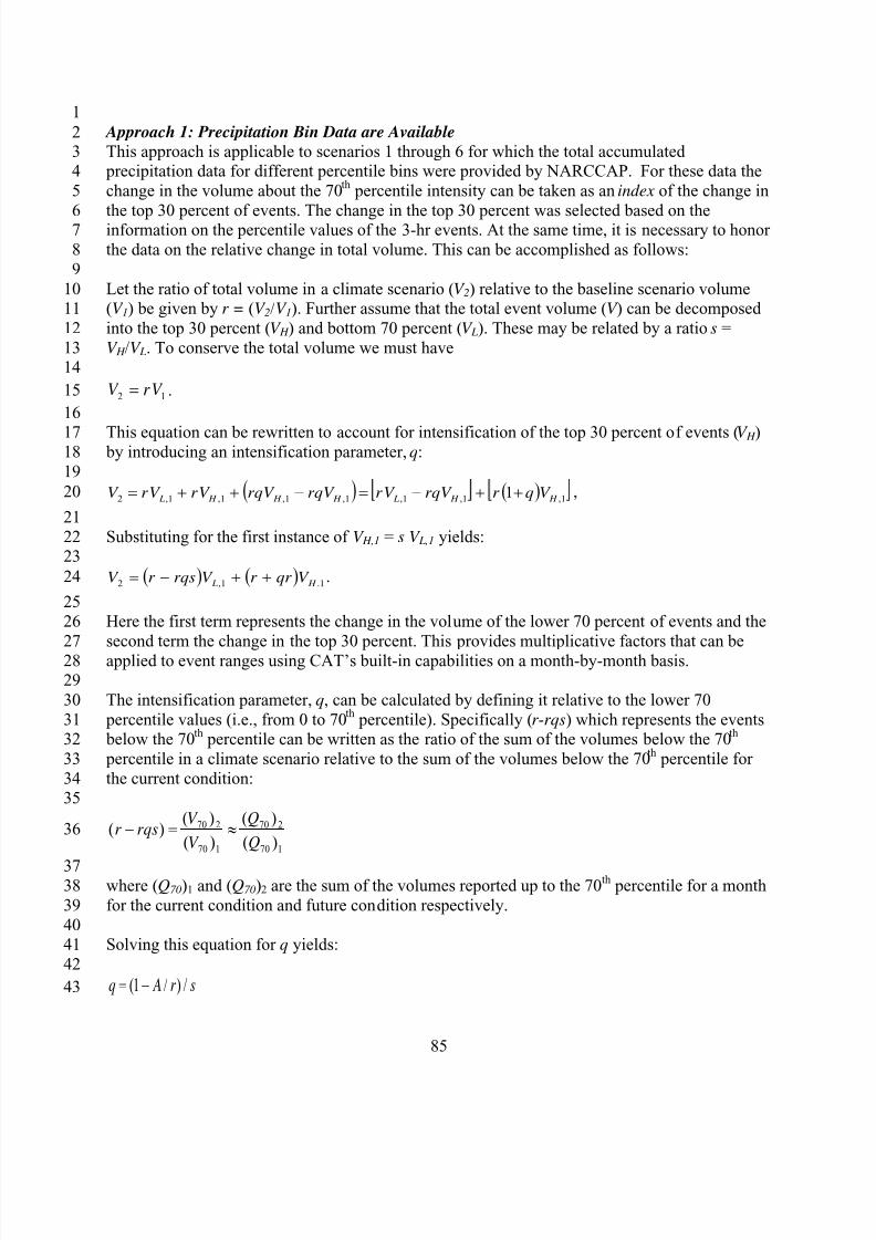
8/13/2019 20 Watersheds Erd
http://slidepdf.com/reader/full/20-watersheds-erd 97/186
5
10
15
20
25
30
35
40
1
234
67
8
9
11
12
1314
16
1718
19
21
2223
24
26
27
2829
3132
33
34
36
3738
39
41
42
43
Approach 1: Precipitation Bin Data are Available
This approach is applicable to scenarios 1 through 6 for which the total accumulated precipitation data for different percentile bins were provided by NARCCAP. For these data the
change in the volume about the 70th
percentile intensity can be taken as an index of the change in
the top 30 percent of events. The change in the top 30 percent was selected based on theinformation on the percentile values of the 3-hr events. At the same time, it is necessary to honor
the data on the relative change in total volume. This can be accomplished as follows:
Let the ratio of total volume in a climate scenario (V 2) relative to the baseline scenario volume(V 1) be given by r = (V 2/V 1). Further assume that the total event volume (V ) can be decomposed
into the top 30 percent (V H ) and bottom 70 percent (V L). These may be related by a ratio s =V H /V L. To conserve the total volume we must have
V 2 = rV 1 .
This equation can be rewritten to account for intensification of the top 30 percent of events (V H ) by introducing an intensification parameter, q:
V = rV + rV + (rqV − rqV ) = rV − rqV + r (1+ q)V ,1 ,2 L,1 H ,1 H ,1 H ,1 L,1 H ,1 H
Substituting for the first instance of V H,1 = s V L,1 yields: V = (r − rqs)V + (r + qr )V . 2 L,1 H .1
Here the first term represents the change in the volume of the lower 70 percent of events and the
second term the change in the top 30 percent. This provides multiplicative factors that can be
applied to event ranges using CAT’s built-in capabilities on a month-by-month basis.
The intensification parameter, q, can be calculated by defining it relative to the lower 70
percentile values (i.e., from 0 to 70th
percentile). Specifically (r -rqs) which represents the events below the 70
th percentile can be written as the ratio of the sum of the volumes below the 70
th
percentile in a climate scenario relative to the sum of the volumes below the 70th
percentile for
the current condition:
(V 70 )2 (Q70 )2(r − rqs) = ≈ (V ) (Q )70 1 70 1
where (Q70)1 and (Q70)2 are the sum of the volumes reported up to the 70th
percentile for a month
for the current condition and future condition respectively.
Solving this equation for q yields:
q = (1− A / r ) / s
85
8/13/2019 20 Watersheds Erd
http://slidepdf.com/reader/full/20-watersheds-erd 98/186
5
10
15
20
25
30
35
40
(Q )where A is defined as A =
70 2
(Q70 )1 In sum, for each month at each station the following were calculated:
V r = 2 from the summary of the climate scenario output,V 1
V s = H from the existing observed precipitation data for the station, sorted into
(V −V H )
events and post-processed to evaluate the top 30 percent (V H ) and bottom70 percent (V L) event volumes. The numerator is calculated as the
difference between total volume and the top 30 percent volume, rather
than directly from V L to correct for analyses in which some scattered precipitation is not included within defined “events.” The s value was
calculated by month and percentile (for every station, every month) using
the observed precipitation time-series data that forms the template for the
delta method representation of future climate time series.
q = (1− A / r ) / s from the summary of the percentile bin climate scenario output summary
The multiplicative adjustment factors for use in the CAT tool can then be assembled as:
r (1 – qs), for the events below the 70th
percentile, andr (1 + q), for the events above the 70
th percentile.
In addition to the typical pattern of intensification of large events, this approach is also sufficientfor the cases where there is a relative increase in the low-percentile intensities. In those cases the
change in the 70th percentile intensity is relatively small and tends to be less than current
conditions under the future scenario, resulting in q being a small negative number. Then,
application of the method results in a decrease in the fraction of the total volume belonging to thelarger events, with a shift to the smaller events – thus approximating observed increases in
intensity for smaller events.
In general, it is necessary to have -1 < q < 1/s to prevent negative solutions to the multipliers.
The condition that q < 1/s is guaranteed to be met by the definition of q (because A/r is always
positive); however, the lower bound condition is not guaranteed to be met. Further, thecalculation of q from the percentile bin data is at best an approximation of the actual
intensification pattern. To address this problem a further constraint is placed on q requiring that
some precipitation must remain in both the high and low ranges after adjustment by requiring-0.8 < q < 0.8/s. It should be noted that the cases in which negative solutions arose were rare and
mainly occurred for stations located in Arizona in the summer months.
Approach 2: Precipitation Bin Data not Available
This approach is applicable for climate scenarios 7 through 14, for which precipitation bin
intensity data were not available. For all these climate scenarios the distribution of volume
1
23
4
6
78
9
11
12
13
14
16
1718
19
21
22
2324
26
2728
29
31
32
3334
3637
38
39
41
42
86
8/13/2019 20 Watersheds Erd
http://slidepdf.com/reader/full/20-watersheds-erd 99/186
changes to events of different sizes is not known. However, as the majority of stations in the
NARCCAP dynamically downscaled scenarios that had precipitation volume increases also
showed strong intensification it was assumed that any increases in precipitation occur in the top30 percent of events. In the cases where there was a decline in precipitation for a given month,
the decreases were applied across all events.
For the case when r = V 2/V 1 > 1 (increasing precipitation), the future volume representing the
climate scenario (V2) can be defined as:
V =* 2 V + 1 L r ⋅V 1 H ,
where r* is the change applied to the upper range (>30%), V H is the volume in the top 30 percent,
and V L is the volume in the bottom 70 percent of events.
Expressing r*= r + ⋅(r −1) ⋅V1 L
V 1 H, the overall change is satisfied, as:
V 2 = V 1 L + r*⋅V 1 H = V 1 L + r ⋅V 1 H - V 1 L + r ⋅V 1 L = r (V 1 H + V 1 L ) = r ⋅ V 1 .
Further, as r > 1, r* is always positive.
For the case of r <= 1 (decreasing precipitation), an across-the-board decrease in precipitation
was applied as follows:
V = r ⋅V + 2 1 L r ⋅V 1 H
The adjustment factors can then be assembled as follows:
For the events above the 70th
percentile, if r > 1, then use r
* r <=1, then use r .
For the events below the 70th
percentile, if r > 1, then use 1 (no change) r <= 1, then use r .
5.1.4.3. Potential Evapotranspiration Changes
Potential evapotranspiration (PET) is simulated with the Penman-Monteith energy balance
method. In addition to temperature and precipitation, the Penman-Monteith method requires as
input dew point (or relative humidity), solar radiation, and wind as inputs. Because only a fewstations have time series for all four additional variables that are complete over the entire 1971
2000 period, these variables are derived from the SWAT 2005 statistical weather generator
(Neitsch et al., 2005). This is done automatically by SWAT. For HSPF implementation astandalone version of the weather generator code was created and used to create time series for
each of the needed variables at each BASINS meteorological station based on the nearest SWAT
weather generator station after applying an elevation correction.
The SWAT weather generator database (.wgn) contains the statistical data needed to generate
representative daily climate data for the different stations. Adjustments to the wgn file
parameters were made using monthly change for the NARCCAP dynamically downscaled
1
2
34
5
67
8
9
10
11
12
13
14
15
1617
18
19
2021
2223
24
2526
2728
2930
31
3233
34
3536
37
3839
40
41
4243
44
45
87
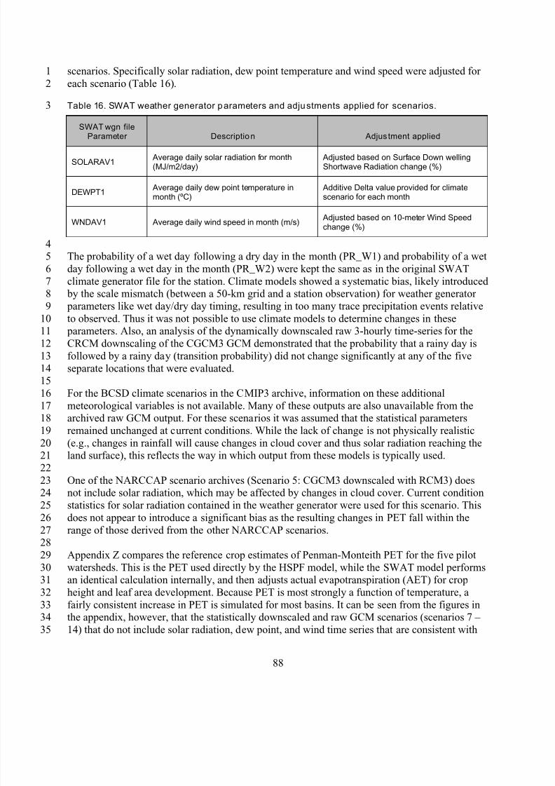
8/13/2019 20 Watersheds Erd
http://slidepdf.com/reader/full/20-watersheds-erd 100/186
1
2
3
scenarios. Specifically solar radiation, dew point temperature and wind speed were adjusted for
each scenario (Table 16).
Table 16. SWAT weather generator parameters and adjustments applied for scenarios.
45
6
78
9
1011
12
13
1415
16
1718
19
2021
22
2324
25
26
2728
293031
32
3334
35
SWAT wgn file
Parameter Description Adjus tment applied
SOLARAV1 Average daily solar radiation for month(MJ/m2/day)
Adjusted based on Surface Down wellingShortwave Radiation change (%)
DEWPT1 Average daily dew point temperature inmonth (ºC)
Additive Delta value provided for climatescenario for each month
WNDAV1 Average daily wind speed in month (m/s) Adjusted based on 10-meter Wind Speedchange (%)
The probability of a wet day following a dry day in the month (PR_W1) and probability of a wet
day following a wet day in the month (PR_W2) were kept the same as in the original SWAT
climate generator file for the station. Climate models showed a systematic bias, likely introduced by the scale mismatch (between a 50-km grid and a station observation) for weather generator
parameters like wet day/dry day timing, resulting in too many trace precipitation events relative
to observed. Thus it was not possible to use climate models to determine changes in these parameters. Also, an analysis of the dynamically downscaled raw 3-hourly time-series for the
CRCM downscaling of the CGCM3 GCM demonstrated that the probability that a rainy day is
followed by a rainy day (transition probability) did not change significantly at any of the five
separate locations that were evaluated.
For the BCSD climate scenarios in the CMIP3 archive, information on these additional
meteorological variables is not available. Many of these outputs are also unavailable from thearchived raw GCM output. For these scenarios it was assumed that the statistical parameters
remained unchanged at current conditions. While the lack of change is not physically realistic
(e.g., changes in rainfall will cause changes in cloud cover and thus solar radiation reaching theland surface), this reflects the way in which output from these models is typically used.
One of the NARCCAP scenario archives (Scenario 5: CGCM3 downscaled with RCM3) doesnot include solar radiation, which may be affected by changes in cloud cover. Current condition
statistics for solar radiation contained in the weather generator were used for this scenario. This
does not appear to introduce a significant bias as the resulting changes in PET fall within the
range of those derived from the other NARCCAP scenarios.
Appendix Z compares the reference crop estimates of Penman-Monteith PET for the five pilotwatersheds. This is the PET used directly by the HSPF model, while the SWAT model performsan identical calculation internally, and then adjusts actual evapotranspiration (AET) for crop
height and leaf area development. Because PET is most strongly a function of temperature, a
fairly consistent increase in PET is simulated for most basins. It can be seen from the figures inthe appendix, however, that the statistically downscaled and raw GCM scenarios (scenarios 7 –
14) that do not include solar radiation, dew point, and wind time series that are consistent with
88
8/13/2019 20 Watersheds Erd
http://slidepdf.com/reader/full/20-watersheds-erd 101/186
1
2
34
5
67
8
9
1011
12
1314
15
16
1718
19
2021
22
2324
25
26
the simulated precipitation and temperature, generally provide noticeably higher estimates of
PET than do the dynamically downscaled models.
A comparison of the effects of data availability on PET calculations can be done through
comparison of scenarios that are based on identical underlying GCM runs for CGCM3 and
GFDL (as discussed in Section 5.1.2. For each of these GCMs there is a pair of dynamicallydownscaled climate scenarios. Annual average PET estimates from these pairs are generally
close to one another, but may differ by up to 4.5 percent from their mean (Table 17). For the
CGCM3 model, PET generated from the raw GCM is similar to that from the dynamically
downscaled scenarios, but PET calculated from the statistically downscaled scenario is from 2 to19 percent higher. This appears to be due to the fact that dew point temperature, which has an
important impact on PET, is provided with the CGCM3 GCM but is not available from the
statistically downscaled CMIP3 product (see Table 15 above). The difference is smallest for theSalt/Verde/San Pedro River basins, where dew point temperature is very low and not expected to
change much under future climates. In contrast, the GFDL model does not provide dew point
temperature from the raw GCM. For that model, both the non-downscaled and statistically
downscaled products produce higher PET estimates than the dynamically downscaled products.As with CGCM3, the smallest effect is seen in the Salt/Verde/San Pedro River basins in Arizona,
and the largest effect in the Susquehanna basin, where a greater change in dew point temperature
and relative humidity is predicted. The observed sensitivity of PET estimates to climate variablesother than air temperature and precipitation suggests that simulation of future climates that does
not account for changes in the full suite of variables that influence PET could thus introduce
significant biases into the simulated water balance.
89
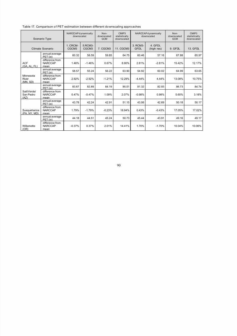
8/13/2019 20 Watersheds Erd
http://slidepdf.com/reader/full/20-watersheds-erd 102/186
Table 17. Comparison o f PET estimation between different do wnscaling appro aches
Scenario Type
NARCCAP d ynamicallydownscaled
Nondownscaled
GCM
CMIP3statisticallydownscaled
NARCCAP d ynamicallydownscaled
Nondownscaled
GCM
CMIP3statisticallydownscaled
Climate Scenario1. CRCMCGCM3
5.RCM3CGCM3 7. CGCM3 11. CGCM3
3. RCM3GFDL
4. GFDL(high res) 9. GFDL 13. GFDL
ACF(GA, AL, FL)
annual averagePET (in)
60.32 58.59 59.85 64.75 60.46 57.16 67.88 65.97
difference fromNARCCAPmean
1.46% -1.46% 0.67% 8.90% 2.81% -2.81% 15.42% 12.17%
MinnesotaRiver(MN, SD)
annual averagePET (in)
58.57 55.24 56.22 63.90 54.92 60.02 64.99 63.65
difference fromNARCCAPmean
2.92% -2.92% -1.21% 12.29% -4.44% 4.44% 13.08% 10.75%
Salt/Verde/San Pedro(AZ)
annual averagePET (in)
83.67 82.89 84.19 85.01 81.32 82.93 86.73 84.74
difference fromNARCCAPmean
0.47% -0.47% 1.09% 2.07% -0.98% 0.98% 5.60% 3.18%
Susquehanna(PA, NY, MD)
annual averagePET (in)
43.78 42.24 42.91 51.15 43.06 42.69 50.18 50.17
difference fromNARCCAPmean
1.79% -1.79% -0.23% 18.94% 0.43% -0.43% 17.05% 17.02%
Willamette(OR)
annual averagePET (in) 44.18 44.51 45.24 50.73 45.44 43.91 49.16 49.17
difference fromNARCCAPmean
-0.37% 0.37% 2.01% 14.41% 1.70% -1.70% 10.04% 10.06%
90
8/13/2019 20 Watersheds Erd
http://slidepdf.com/reader/full/20-watersheds-erd 103/186
1
2
3
45
678
9
10
1112
13
1415
16
17
1819
20
2122
23
2425
26
27
2829
30
3132
33
3435
36
3738
394041
42
43
44
45
5.2. URBAN DEVELOPMENT SCENARIOS
The impacts of urban and residential development on watersheds are pervasive and widespread
at the national scale. The relative effects of future climate change and urban and residentialdevelopment on watersheds has important management implications. Moreover, because climate
and urban development can result in similar types of impacts, e.g. higher peaks and lower lowflow conditions, the management of land use impacts is a potentially important adaptive strategyfor increasing resilience to climate change (Pyke et al., 2011).
5.2.1. Land Use Scenarios
In this study two land use scenarios were evaluated in each study area: a baseline scenariorepresenting current (2001) conditions and a future scenario representing mid-21
stcentury
changes in urban and residential land. Projected changes in urban and residential development
were acquired from EPA’s Integrated Climate and Land Use Scenarios (ICLUS) project (U.S.EPA, 2009d). ICLUS has produced seamless, national-scale change scenarios for developed land
that are compatible with the assumptions about population growth and migration that underlie
the IPCC greenhouse gas emissions storylines. These scenarios were developed using a
demographic model, consisting of a cohort-component model and gravity model, to estimatefuture population through 2100 for each county in the conterminous U.S. The resulting
population is allocated to 1-hectare pixels, by county, using the spatial allocation model
SERGoM (Spatially Explicit Regional Growth Model). The final spatial dataset provides decadal projections of housing density and impervious surface cover for the period 2000 through 2100.
Data from the ICLUS project are composed of grid-based housing density estimates with 100-mcells, whose values are set equal to units/ha x 1,000. Existing housing densities were estimated
using a variety of sources and models, and future housing densities developed under various
scenarios for each decade through 2100. For the existing housing density grid, two types of
“undevelopable” area where residential developed was precluded were masked out during the production – a comprehensive spatial dataset of protected lands (including land placed in
conservation easements), and land assumed to be commercial/industrial under current conditions.
Undevelopable commercial/industrial land use was masked out according to the SERGoMmethod (U.S. EPA, 2009d) that eliminated commercial, industrial, and transportation areas that
preclude residential development, identified as “locations (1 ha cells) that had >25% urban/built
up land cover but that also had lower than suburban levels of housing density.”
The ICLUS projections used in this study thus do not account for potential growth in
commercial/industrial land use. It is also important to note that the ICLUS projections do notexplicitly account for changes in rural or agricultural land uses. These categories change only to
the extent that they are predicted to convert to developed land.
5.2.2. Translating ICLUS Land Use Projections to Watershed Model Inputs
The ICLUS projections used in this study are for changes in housing density and impervious
cover. This data cannot be used directly with the SWAT and HSPF watershed models which
require land use data consistent with the NLCD. It was therefore necessary to translate between
ICLUS projections and NLCD land use classes.
91
8/13/2019 20 Watersheds Erd
http://slidepdf.com/reader/full/20-watersheds-erd 104/186
1
2
34
5
67
8
9
1011
12
1314
15
16
1718
19
2021
22
2324
25
2627
28
2930
31
32
3334
35
3637
38
3940
41
42
4344
45
46
The baseline (2001) and future (2050) land use scenarios are referred to as “L0” and “L1”,
respectively. Baseline land use, derived from the 2001 NLCD, contains four developed landclassifications (NLCD classes 21 through 24), nominally representing “developed, open space”
(less than 20 percent impervious), developed, low intensity (20 – 49 percent impervious),
developed, medium intensity (50 – 79 percent impervious), and developed, high density (greaterthan 80 percent impervious). Impervious fractions within each developed NLCD land use class
were estimated separately for each study area, using the 2001 NLCD Land Cover and Urban
Impervious data products. ICLUS land use change projections were implemented by modifying
the existing land use distribution in the watershed models.
ICLUS estimates housing density on a continuous scale. To process the data more efficiently, the
data were reclassified into ten housing density ranges.
In each study area, the ICLUS housing density ranges were cross-tabulated with NLCD 2001
classes based on percent imperviousness. It was assumed that the number of housing units
changes, but that the characteristic percent impervious values for each NLCD developed classremains constant. The change in land area needed to account for the change in impervious area
was then back calculated.
ICLUS housing density class estimates and the NLCD developed classes do not have a one-to
one spatial relationship because they are constructed on different underlying scales. ICLUS
represents housing density based largely on the scale of census block groups. As a result, itrepresents the overall density within a relatively large geographic area when compared to the
30x30 meter resolution of NLCD 2001 land cover and can represent a mix of different NLCD
classes. Therefore, land use changes must be evaluated on a spatially aggregated basis at thescale of model subbasins.
The gains (and losses) in NLCD class interpreted from ICLUS were tabulated separately for eachsubbasin. In almost every case, the gains far exceeded the losses and a net increase was predicted
in all four NLCD developed classes. However, there were a few cases where there was an overall
loss of the lowest density NLCD class. This tended to occur when a subbasin was already built
out, and ICLUS predicted redevelopment at a higher density.
To represent the net change in future land cover, the developed land use was added (or
subtracted) from the existing totals in each subbasin. Land area was then removed from eachundeveloped NLCD class (excluding water and wetlands) according to their relative ratios in
each subbasin to account for increases in developed area. If the undeveloped land area was not
sufficient to accommodate the projected growth, development on wetlands was allowed. Thereductions in undeveloped land were distributed proportionately among modeled soils (in
SWAT) or hydrologic soil groups (in HSPF). The new developed lands were then assumed to
have the parameters of the most dominant soil and lowest HRU slope in the sub-basin. For
HSPF, the changed area was implemented directly in the SCHEMATIC block of the user controlinput (.uci) file. For SWAT, the land use change was implemented by custom VBA code that
directly modified the SWAT geodatabase that creates the model input files.
92
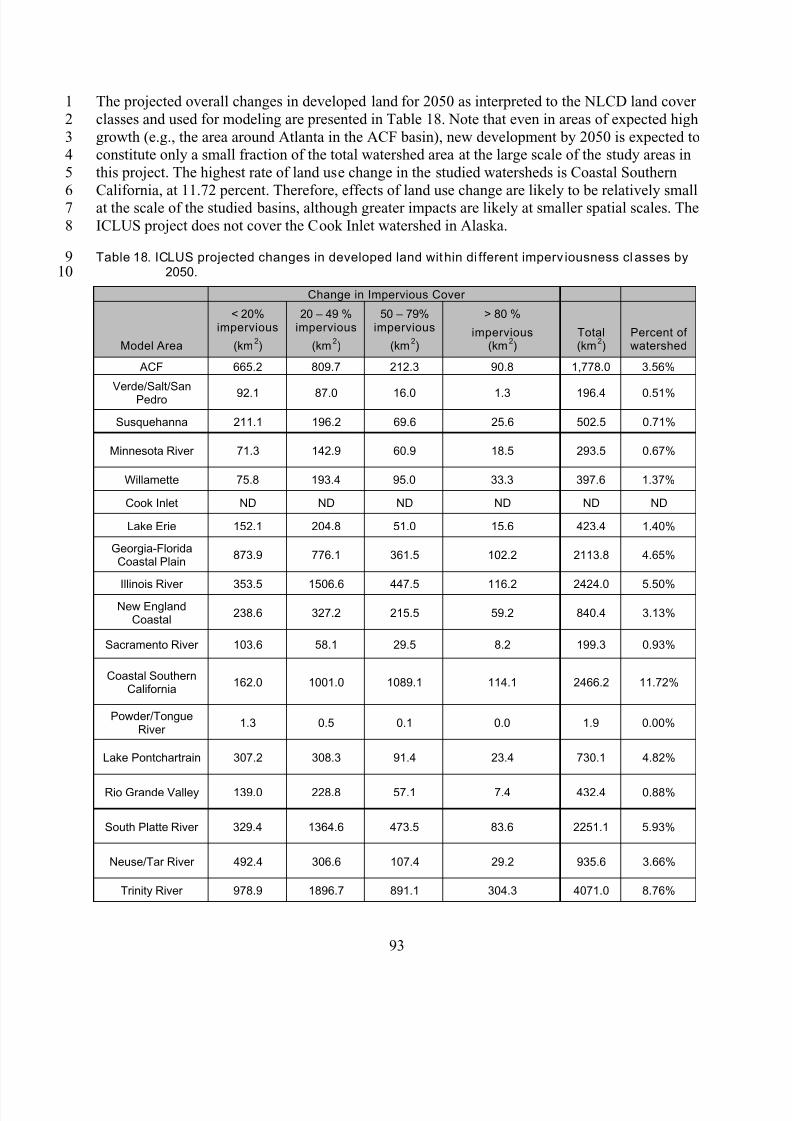
8/13/2019 20 Watersheds Erd
http://slidepdf.com/reader/full/20-watersheds-erd 105/186
1 The projected overall changes in developed land for 2050 as interpreted to the NLCD land cover
classes and used for modeling are presented in Table 18. Note that even in areas of expected high
growth (e.g., the area around Atlanta in the ACF basin), new development by 2050 is expected toconstitute only a small fraction of the total watershed area at the large scale of the study areas in
this project. The highest rate of land use change in the studied watersheds is Coastal Southern
California, at 11.72 percent. Therefore, effects of land use change are likely to be relatively smallat the scale of the studied basins, although greater impacts are likely at smaller spatial scales. The
ICLUS project does not cover the Cook Inlet watershed in Alaska.
Table 18. ICLUS projected changes in developed land within di fferent imperv iousness classes by2050.
2
34
5
67
8
910
93
Change in Impervious Cover
Model Area
< 20%impervious
(km2)
20 – 49 %impervious
(km2)
50 – 79%impervious
(km2)
> 80 %
impervious(km
2)
Total(km
2)
Percent ofwatershed
ACF 665.2 809.7 212.3 90.8 1,778.0 3.56%
Verde/Salt/SanPedro 92.1 87.0 16.0 1.3 196.4 0.51%
Susquehanna 211.1 196.2 69.6 25.6 502.5 0.71%
Minnesota River 71.3 142.9 60.9 18.5 293.5 0.67%
Willamette 75.8 193.4 95.0 33.3 397.6 1.37%
Cook Inlet ND ND ND ND ND ND
Lake Erie 152.1 204.8 51.0 15.6 423.4 1.40%
Georgia-FloridaCoastal Plain
873.9 776.1 361.5 102.2 2113.8 4.65%
Illinois River 353.5 1506.6 447.5 116.2 2424.0 5.50%New England
Coastal238.6 327.2 215.5 59.2 840.4 3.13%
Sacramento River 103.6 58.1 29.5 8.2 199.3 0.93%
Coastal SouthernCalifornia
162.0 1001.0 1089.1 114.1 2466.2 11.72%
Powder/TongueRiver
1.3 0.5 0.1 0.0 1.9 0.00%
Lake Pontchartrain 307.2 308.3 91.4 23.4 730.1 4.82%
Rio Grande Valley 139.0 228.8 57.1 7.4 432.4 0.88%
South Platte River 329.4 1364.6 473.5 83.6 2251.1 5.93%
Neuse/Tar River 492.4 306.6 107.4 29.2 935.6 3.66%
Trinity River 978.9 1896.7 891.1 304.3 4071.0 8.76%

8/13/2019 20 Watersheds Erd
http://slidepdf.com/reader/full/20-watersheds-erd 106/186
Loup/Elkhorn River 8.9 18.7 4.1 1.6 33.2 0.06%
Upper ColoradoRiver
56.9 168.1 66.3 8.3 299.6 0.65%
1
2
3
4
94
8/13/2019 20 Watersheds Erd
http://slidepdf.com/reader/full/20-watersheds-erd 107/186
5
10
15
20
25
30
35
40
1 6. RESULTS IN PILOT WATERSHEDS: SENSITIVITY TO DIFFERENT
METHODOLOGICAL CHOICES
One goal of this study was to assess the implications of different methodological choices forconducting climate change impacts assessments on the variability of simulation results. This
assessment was based on simulations in 5 Pilot study areas. The five pilot study basins are the
Minnesota River, Apalachicola-Chattahoochee-Flint (ACF), Susquehanna, Willamette, andVerde/ Salt/ San Pedro Rivers). In each of the 5 pilot sites, independent simulations were
conducted using the SWAT and HSPF watershed models, and in addition to the 6 dynamically
downscaled NARCCAP scenarios, an additional set of climate change scenarios was evaluated,four based on the statistically downscaled BCSD dataset, and four based directly on GCMs with
no downscaling. These simulations in Pilot sites allow assessment of the variability resulting
from use of different watershed models, and variability resulting from use climate change
scenarios developed using different downscaling methods. This level of effort was not feasible atall 20 sites due to resource limitations. A reduced modeling effort was conducted at the
remaining 15 non-pilot sites. The more detailed analysis at Pilot sites was completed before
initiating work at the other 15 sites, and results of this assessment were used to informdevelopment of the reduced effort modeling conducted non-pilot sites. This section is a summary
of results in the pilot study areas.
6.1. COMPARISON OF WATERSHED MODELS
Two different watershed models, SWAT and HSPF, were calibrated and applied to the five pilot
study areas (the Willamette, Central Arizona, Minnesota (Upper Mississippi), Apalachicola
Chattahoochee-Flint (ACF), and Susquehanna basins). Evaluation of different watershed modelscan be considered an extension of the scenario-based, ensemble approach commonly used in
climate change studies. The magnitude of the additional variability introduced by choice of a
hydrologic model is of interest when simulating hydrologic responses to climate change andurban development.
This section provides a summary of the relative performance of the two models, along with
theoretical and practical considerations, concluding with the rationale for selecting the SWATmodel to implement in the remaining 15 non-pilot watersheds. Detailed examination of the
calibration of each model in the five pilot study areas and the results of change scenarios
conducted with each model are presented in separate sections.
Both HSPF and SWAT are public domain, government-supported models with a long history of
application. Yet, they also take a rather different approach to watershed simulation and have
different structures and algorithms, resulting in different strengths and weaknesses. Mostnotably, the two models differ in the way that they represent infiltration and plant-climate
interactions. SWAT (in standard application mode) simulates rainfall-runoff processes using a
Curve Number approach, operating at a daily time step. The Curve Number approach first partitions incoming moisture in to direct runoff and a remainder that is available for infiltration.
In contrast, HSPF simulates rainfall-runoff processes using Green-Ampt infiltration, in which
infiltration into the soil is simulated first, with the remainder available for direct runoff or surfacestorage.
2
34
67
8
9
11
12
1314
1617
18
19
21
22
2324
2627
28
29
31
32
3334
36
3738
39
41
42
4344
95
8/13/2019 20 Watersheds Erd
http://slidepdf.com/reader/full/20-watersheds-erd 108/186
1
2
34
5
67
8
9
10
11
12
13
1415
16
17
1819
20
2122
23
2425
26
27
2829
30
3132
33
3435
36
3738
3940
4142
43
4445
46
HSPF is typically run at a sub-daily time step, usually hourly for large watersheds, and has a
more sophisticated representation of runoff, infiltration, and channel transport processes thandoes SWAT. SWAT’s advantage is that it incorporates a plant growth model (including
representation of CO2 fertilization) and can therefore simulate some of the important feedbacks
between plant growth and hydrologic response. Both models simulate evapotranspiration of soilwater stores, but HSPF does this using empirical monthly coefficients relative to potential
evapotranspiration, while SWAT incorporates a plant growth model that can, in theory,
dynamically represent plant transpiration of soil moisture.
6.1.1. Influence of Calibration Strategies
Model implementation, calibration, and validation was conducted in accordance with the
modeling Quality Assurance Project Plan (QAPP) (see Appendix B; Tetra Tech, 2008) for each
of the five pilot study areas. Development and setup of the two watershed models proceededfrom a common basis, with both models using the same sub-basin delineations, land use
coverage (2001 NLCD), soils coverage (STATSGO), hydrography, digital elevation model,
impervious area fractions for developed land classes, and point source and dam representations.
Other aspects of model setup were designed to be similar, although not identical. For instance,hydrologic response units (the fundamental building blocks of the upland simulation) were
created as an overlay of land use and hydrologic soil group (HSG) for HSPF, while SWAT uses
an overlay of land use and STATSGO dominant soil, associating various other properties inaddition to HSG with the model hydrologic response units.
Both models also used the same calibration/validation locations and observed data series, and both initiated calibration at the same location. Further, the calibration of both models was guided
by pre-specified statistical analyses that were performed using identical spreadsheet setups
obtained from a common template. Despite these commonalities, the different models were
developed by different research teams, with inevitable differences in results. Model calibrationassignments were intentionally structured so that the same team did not apply both HSPF and
SWAT to a single study area, and each watershed model was implemented by at least three
different modeling teams for the pilot studies.
One key reason for differences in results is the extent to which spatial calibration of the model
was pursued, which was left to modeler judgment. In all study areas, initial calibration andvalidation was pursued at an “initial calibration” gage and monitoring station at an HUC8 spatial
scale. The calibration results were then carried to the larger study area. At this point, individual
modeler preferences introduced some variability into results. Some modelers undertook detailedspatial adjustments to parameters; others extended the initial parameter set with only minor
modifications. With more spatial adjustments a higher degree of fit is generally to be expectedfor model calibration – although this does not necessarily result in better performance in model
validation. In general, limited spatial calibration adjustments beyond the parameter set obtainedat the initial location was carried out for the Minnesota River, Susquehanna, and Willamette
SWAT models and also for the Susquehanna HSPF model.
Another cause of different performance is the existence of prior modeling efforts in the basin.
There were existing detailed HSPF models for the Susquehanna, ACF, and Minnesota River
96
8/13/2019 20 Watersheds Erd
http://slidepdf.com/reader/full/20-watersheds-erd 109/186
1
2
34
5
67
8
9
10
11
12
13
1415
16
1718
19
2021
22
23
2425
26
27
2829
3031
32
3334
35
36
basins, while SWAT models existed for the Minnesota River and Central Arizona basins. Where
prior models existed they influenced calibration of the models used in this study – even though
the spatial basis and representation of evapotranspiration typically differed from the earliermodels.
The net effect of these factors is that the results should not be interpreted as a true head-to-headcomparison of the two models, as the results for any given watershed may be skewed by
exogenous factors such as modeler calibration strategy. Instead, it is most relevant to examine
relative performance and potential inconsistencies between simulations using the two models.
6.1.2. Comparison of Model Calibration and Validation Performance
Models were calibrated and validated using multiple measures as summarized previously in this
report and described in full detail in Appendices D - W. Model performance was evaluated based
on ability to represent a variety of flow statistics and monthly loads of nitrogen, phosphorus, andsuspended sediment. This section examines hydrologic simulations as compared to observed
flow records based on total volume error and the daily Nash-Sutcliffe coefficient of model fit
efficiency. Model performance is first examined in terms of the quality of fit for the initialcalibration watershed followed by similar analyses for the largest-scale downstream watershed.
Inter-comparisons then provide some insight into model performance relative to temporal change
(calibration versus validation period) and relative to spatial change within each study area(calibration watershed versus downstream watershed).
6.1.2.1. Streamflow Results
Summary results for percent error in total volume and the Nash-Sutcliffe E coefficient for dailyflows are shown in Table 19 and Table 20, respectively, for the initial calibration site along with
the calibration fit for the most downstream gage in the watershed. In general, the quality of
model fit is good for both models. In most, but not all cases, the quality of model fit is slightly
better (smaller magnitude of percent error, larger E coefficient) for the HSPF simulations (e.g.,Figure 25 for the calibration period). This is likely due in large part to the use of daily
precipitation in SWAT versus hourly precipitation in HSPF, although the advantage accruing toHSPF is muted by the fact that many of the “hourly” precipitation input series used are actually
disaggregated from daily totals. Monthly values of Nash-Sutcliffe E are higher for both models,
but attention is called to the daily scale as this better reflects the models’ ability to separatesurface and subsurface flow pathways. Note that E is low for the Arizona initial site on the Verde
River because flow is dominated by relatively constant deep groundwater discharges.
97
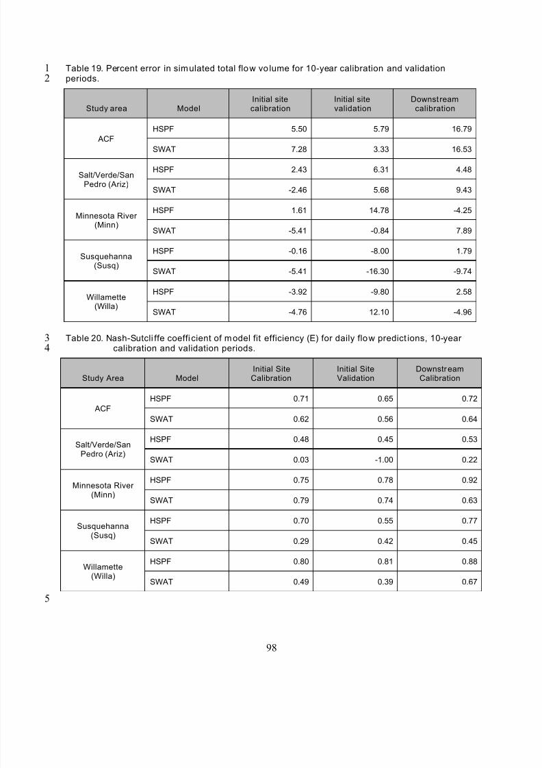
8/13/2019 20 Watersheds Erd
http://slidepdf.com/reader/full/20-watersheds-erd 110/186
1 Table 19. Percent error in simulated total flow vo lume for 10-year calibration and validation
periods.2
3
Initial site Initial site Downst reamStudy area Model calibration validation calibration
HSPF 5.50 5.79 16.79
ACF
SWAT 7.28 3.33 16.53
Salt/Verde/SanPedro (Ariz)
HSPF 2.43 6.31 4.48
SWAT -2.46 5.68 9.43
Minnesota River(Minn)
HSPF 1.61 14.78 -4.25
SWAT -5.41 -0.84 7.89
Susquehanna
(Susq)
HSPF -0.16 -8.00 1.79
SWAT -5.41 -16.30 -9.74
Willamette(Willa)
HSPF -3.92 -9.80 2.58
SWAT -4.76 12.10 -4.96
Table 20. Nash-Sutcli ffe coeffi cient of model fit efficiency (E) for daily flow predict ions, 10-yearcalibration and validation periods.4
5
98
Initial Site Initial Site DownstreamStudy Area Model Calibration Validation Calibration
HSPF 0.71 0.65 0.72
ACF
SWAT 0.62 0.56 0.64
Salt/Verde/SanPedro (Ariz)
HSPF 0.48 0.45 0.53
SWAT 0.03 -1.00 0.22
Minnesota River(Minn)
HSPF 0.75 0.78 0.92
SWAT 0.79 0.74 0.63
Susquehanna
(Susq)
HSPF 0.70 0.55 0.77
SWAT 0.29 0.42 0.45
Willamette(Willa)
HSPF 0.80 0.81 0.88
SWAT 0.49 0.39 0.67
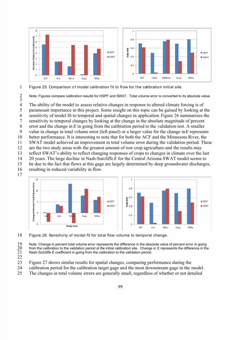
8/13/2019 20 Watersheds Erd
http://slidepdf.com/reader/full/20-watersheds-erd 111/186
1
2345
6
78
9
1011
12
1314
15
16
17
18
19202122
2324
25
0
0 .2
0 .4
0 .6
0 .8
1
ACF CeAZ MNRive r Susq Willm
D a i l y N S E
HSPF
SWAT
Figure 25. Comparison o f model calibration f it to fl ow for the calibration initi al site.
Note: Figures compare calibration results for HSPF and SWAT. Total volume error is converted to its absolute value.
The ability of the model to assess relative changes in response to altered climate forcing is of paramount importance in this project. Some insight on this topic can be gained by looking at the
sensitivity of model fit to temporal and spatial changes in application. Figure 26 summarizes the
sensitivity to temporal changes by looking at the change in the absolute magnitude of percenterror and the change in E in going from the calibration period to the validation test. A smaller
value in change in total volume error (left panel) or a larger value for the change in E represents
better performance. It is interesting to note that for both the ACF and the Minnesota River, theSWAT model achieved an improvement in total volume error during the validation period. These
are the two study areas with the greatest amount of row crop agriculture and the results may
reflect SWAT’s ability to reflect changing responses of crops to changes in climate over the last20 years. The large decline in Nash-Sutcliffe E for the Central Arizona SWAT model seems to
be due to the fact that flows at this gage are largely determined by deep groundwater discharges,
resulting in reduced variability in flow.
99
Figure 26. Sensitivi ty of model fit for total flow volume to temporal change.
Note: Change in percent total volume error represents the difference in the absolute value of percent error in goingfrom the calibration to the validation period at the initial calibration site. Change in E represents the difference in theNash-Sutcliffe E coefficient in going from the calibration to the validation period.
Figure 27 shows similar results for spatial changes, comparing performance during thecalibration period for the calibration target gage and the most downstream gage in the model.
The changes in total volume errors are generally small, regardless of whether or not detailed
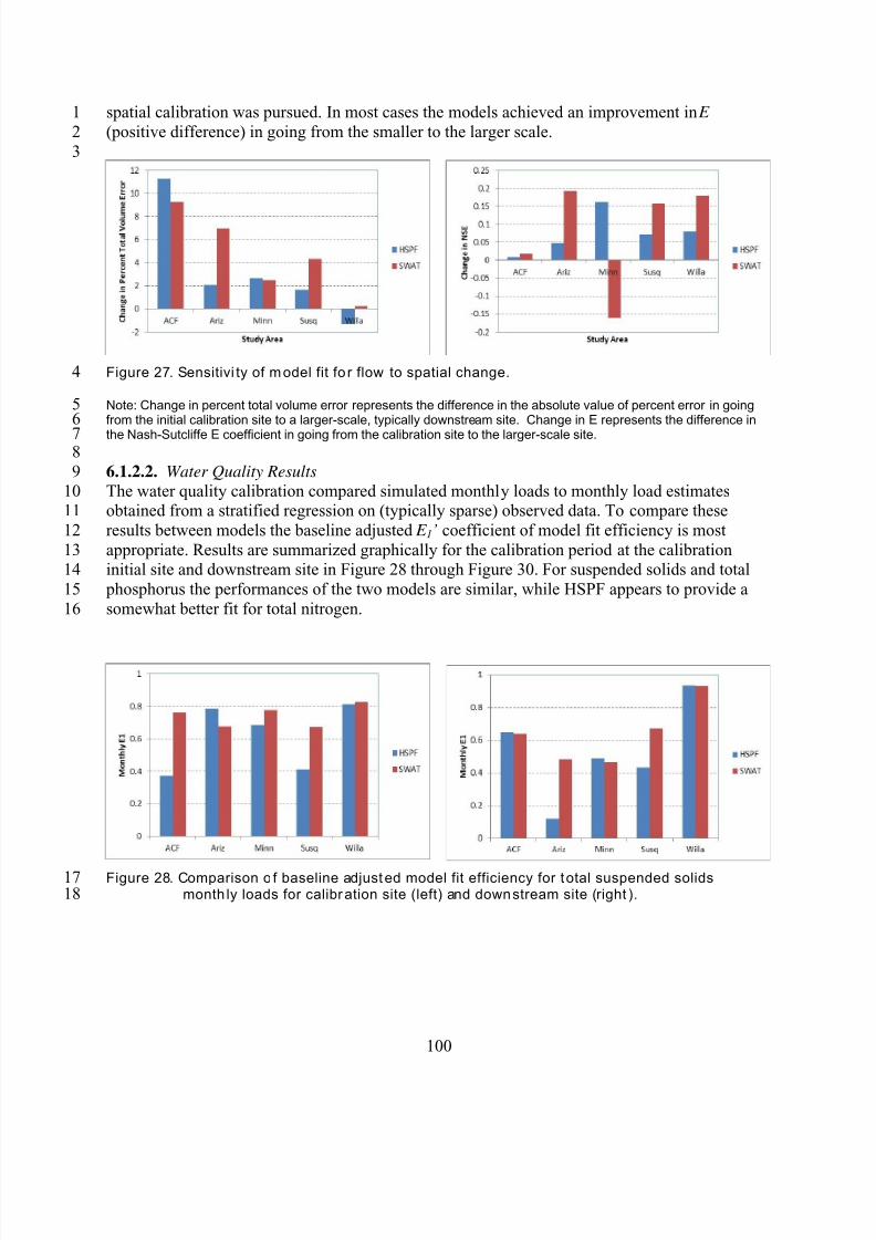
8/13/2019 20 Watersheds Erd
http://slidepdf.com/reader/full/20-watersheds-erd 112/186
1 spatial calibration was pursued. In most cases the models achieved an improvement in E
(positive difference) in going from the smaller to the larger scale.2
3
4
56
78
91011
12
1314
15
16
17
Figure 27. Sensitivi ty of model fit fo r flow to spatial change.
Note: Change in percent total volume error represents the difference in the absolute value of percent error in goingfrom the initial calibration site to a larger-scale, typically downstream site. Change in E represents the difference in
the Nash-Sutcliffe E coefficient in going from the calibration site to the larger-scale site.
6.1.2.2. Water Quality Results
The water quality calibration compared simulated monthly loads to monthly load estimatesobtained from a stratified regression on (typically sparse) observed data. To compare these
results between models the baseline adjusted E 1’ coefficient of model fit efficiency is most
appropriate. Results are summarized graphically for the calibration period at the calibrationinitial site and downstream site in Figure 28 through Figure 30. For suspended solids and total
phosphorus the performances of the two models are similar, while HSPF appears to provide a
somewhat better fit for total nitrogen.
Figure 28. Comparison o f baseline adjusted model fit efficiency for total suspended solidsmonth ly loads for calibration site (left) and downstream site (right ).18
100
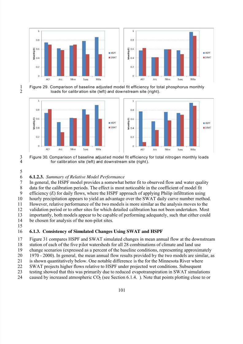
8/13/2019 20 Watersheds Erd
http://slidepdf.com/reader/full/20-watersheds-erd 113/186
34
56
789
10
1112
13
1415
16
171819
20
21
2223
24
12
Figure 29. Comparison of baseline adjusted model fit efficiency for total phosphorus monthlyloads for calibr ation site (left) and downstream site (right).
101
Figure 30. Comparison o f baseline adjusted model fit efficiency for total nitrogen monthly loadsfor calibration site (left) and downstream site (right ).
6.1.2.3. Summary of Relative Model Performance
In general, the HSPF model provides a somewhat better fit to observed flow and water qualitydata for the calibration periods. The effect is most noticeable in the coefficient of model fitefficiency ( E ) for daily flows, where the HSPF approach of applying Philip infiltration using
hourly precipitation appears to yield an advantage over the SWAT daily curve number method.
However, relative performance of the two models is more similar as the analysis moves to thevalidation period or to other sites for which detailed calibration has not been undertaken. Most
importantly, both models appear to be capable of performing adequately, such that either could
be chosen for analysis of the non-pilot sites.
6.1.3. Consistency of Simulated Changes Using SWAT and HSPF
Figure 31 compares HSPF and SWAT simulated changes in mean annual flow at the downstreamstation of each of the five pilot watersheds for all 28 combinations of climate and land usechange scenarios (expressed as a percent of the baseline conditions, representing approximately
1970 - 2000). In general, the mean annual flow results provided by the two models are similar, as
is shown quantitatively below. One notable difference is the for the Minnesota River where
SWAT projects higher flows relative to HSPF under projected wet conditions. Subsequenttesting showed that this was primarily due to reduced evapotranspiration in SWAT simulations
caused by increased atmospheric CO2 (see Section 6.1.4. ). Note that points plotting close to or
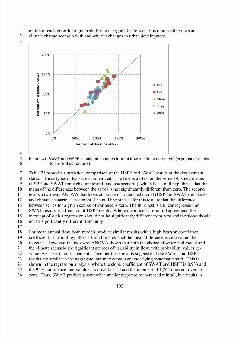
8/13/2019 20 Watersheds Erd
http://slidepdf.com/reader/full/20-watersheds-erd 114/186
1
2
3
4
56
7
89
1011
12
1314
15
1617
18
192021
22
2324
25
26
on top of each other for a given study site in Figure 31 are scenarios representing the same
climate change scenario with and without changes in urban development.
0%
50%
100%
150%
200%
0% 50% 100% 150% 200%
P e r c e n t o f B a s e l i n e - S W A T
Percent of Baseline - HSPF
ACF
Ariz
Minn
Susq
Willa
Figure 31. SWAT and HSPF simulated changes in total fl ow in pilot watersheds (expressed relativeto current conditions).
Table 21 provides a statistical comparison of the HSPF and SWAT results at the downstream
station. Three types of tests are summarized. The first is a t-test on the series of paired means(HSPF and SWAT for each climate and land use scenario), which has a null hypothesis that the
mean of the differences between the series is not significantly different from zero. The secondtest is a two-way ANOVA that looks at choice of watershed model (HSPF or SWAT) as blocks
and climate scenario as treatment. The null hypotheses for this test are that the difference
between series for a given source of variance is zero. The third test is a linear regression onSWAT results as a function of HSPF results. Where the models are in full agreement, the
intercept of such a regression should not be significantly different from zero and the slope should
not be significantly different from unity.
For mean annual flow, both models produce similar results with a high Pearson correlation
coefficient. The null hypothesis from the t-test that the mean difference is zero cannot berejected. However, the two-way ANOVA shows that both the choice of watershed model andthe climate scenario are significant sources of variability in flow, with probability values (p
value) well less than 0.1 percent. Together these results suggest that the SWAT and HSPF
results are similar in the aggregate, but may contain an underlying systematic shift. This isshown in the regression analysis, where the slope coefficient of SWAT and HSPF is 0.933 and
the 95% confidence interval does not overlap 1.0 and the intercept of 1,262 does not overlap
zero. Thus, SWAT predicts a somewhat smaller response to increased rainfall, but results in
102
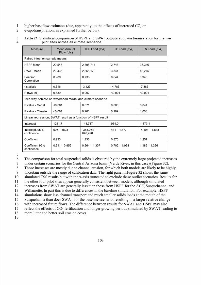
8/13/2019 20 Watersheds Erd
http://slidepdf.com/reader/full/20-watersheds-erd 115/186
1
2
34
5
6
78
9
1011
12
1314
1516
1718
19
higher baseflow estimates (due, apparently, to the effects of increased CO2 on
evapotranspiration, as explained further below).
Table 21. Statisti cal comparison of HSPF and SWAT outputs at downs tream station for the fivepilot sites across all climate scenarios
Measure Mean AnnualFlow (cfs) TSS Load (t/yr)
Paired t-test on sample means
TP Load (t/yr) TN Load (t/yr)
HSPF Mean 20,546 2,398,714 2,748 35,346
SWAT Mean 20.435 2,865,178 3,344 43,275
PearsonCorrelation
0.989 0.733 0.644 0.948
t-statistic 0.616 -3.123 -4.783 -7.385
P (two-tail) 0.539 0.002 <0.001 <0.001
Two-way ANOVA on watershed model and climate scenario
P value - Model <0.001 0.071 0.006 0.044
P value - Climate <0.001 0.960 0.999 1.000
Linear regression; SWAT result as a function of HSPF result
Intercept 1261.7 141,717 954.0 -1173.1
Intercept, 95 %confidence
695 – 1828 -363,064 –646,498
431 – 1,477 -4,194 – 1,848
Coefficient 0.933 1.136 0.870 1.257
Coefficient 95%
confidence
0.911 – 0.956 0.964 – 1.307 0.702 – 1.038 1.189 – 1.326
The comparison for total suspended solids is obscured by the extremely large projected increases
under certain scenarios for the Central Arizona basin (Verde River, in this case) (Figure 32).Those increases are mostly due to channel erosion, for which both models are likely to be highly
uncertain outside the range of calibration data. The right panel in Figure 32 shows the same
simulated TSS results but with the x-axis truncated to exclude these outlier scenarios. Results forthe other four pilot sites appear generally consistent between models, although simulated
increases from SWAT are generally less than those from HSPF for the ACF, Susquehanna, and
Willamette. In part this is due to differences in the baseline simulation. For example, HSPFsimulations show less channel transport and much smaller solids loads at the mouth of the
Susquehanna than does SWAT for the baseline scenario, resulting in a larger relative changewith increased future flows. The difference between results for SWAT and HSPF may also
reflect the effects of CO2 fertilization and longer growing periods simulated by SWAT leading tomore litter and better soil erosion cover.
103
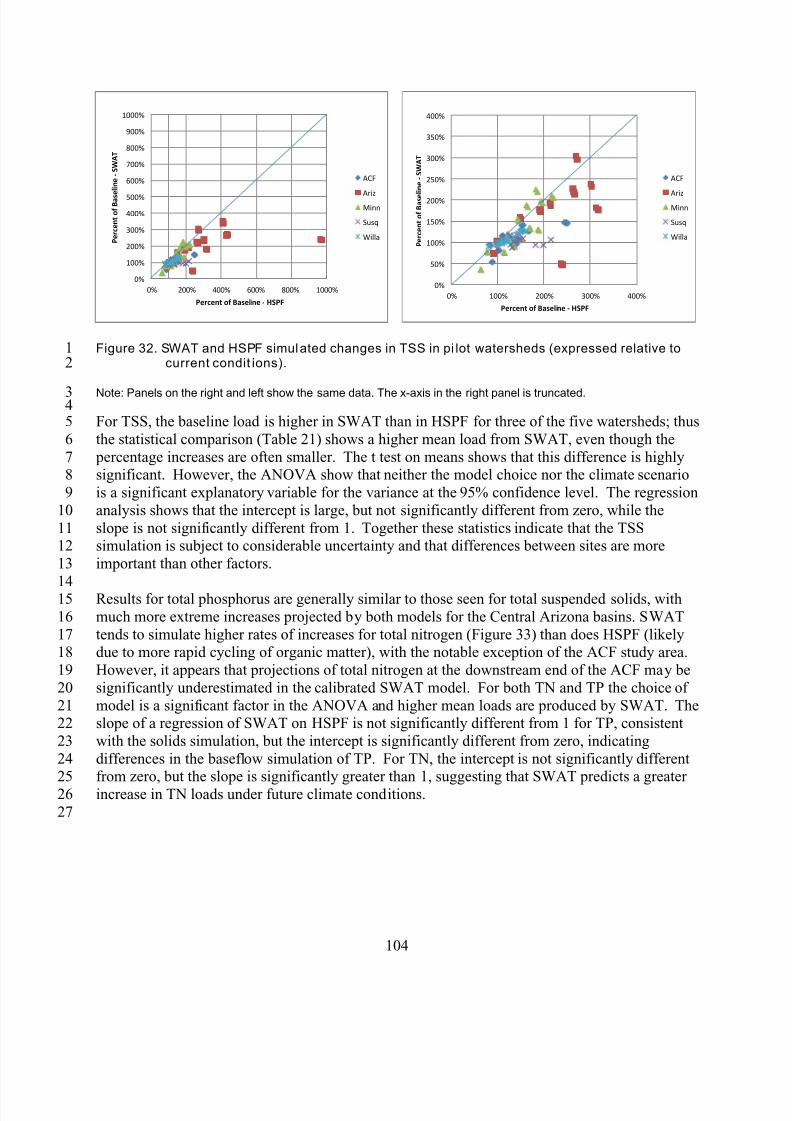
8/13/2019 20 Watersheds Erd
http://slidepdf.com/reader/full/20-watersheds-erd 116/186
0%
100%
200%
300%
400%
500%
600%
700%
800%
900%
1000%
0%
P e r c e n t o f B a s e l i n e - S W A T
200% 400% 600% 800% 1000%
Percent of Baseline - HSPF
ACF
ArizMinn
Susq
Willa
0%
50%
100%
150%
200%
250%
300%
350%
400%
0%
P e r c e n t o f B a s e
l i n e - S W A T
100% 200% 300% 400%
Percent of Baseline - HSPF
ACF
ArizMinn
Susq
Willa
12
Figure 32. SWAT and HSPF simulated changes in TSS in pi lot watersheds (expressed relative tocurrent condit ions).
Note: Panels on the right and left show the same data. The x-axis in the right panel is truncated.
For TSS, the baseline load is higher in SWAT than in HSPF for three of the five watersheds; thus
the statistical comparison (Table 21) shows a higher mean load from SWAT, even though the
percentage increases are often smaller. The t test on means shows that this difference is highlysignificant. However, the ANOVA show that neither the model choice nor the climate scenario
is a significant explanatory variable for the variance at the 95% confidence level. The regression
analysis shows that the intercept is large, but not significantly different from zero, while the
slope is not significantly different from 1. Together these statistics indicate that the TSSsimulation is subject to considerable uncertainty and that differences between sites are more
important than other factors.
Results for total phosphorus are generally similar to those seen for total suspended solids, with
much more extreme increases projected by both models for the Central Arizona basins. SWAT
tends to simulate higher rates of increases for total nitrogen (Figure 33) than does HSPF (likelydue to more rapid cycling of organic matter), with the notable exception of the ACF study area.
However, it appears that projections of total nitrogen at the downstream end of the ACF may be
significantly underestimated in the calibrated SWAT model. For both TN and TP the choice of
model is a significant factor in the ANOVA and higher mean loads are produced by SWAT. Theslope of a regression of SWAT on HSPF is not significantly different from 1 for TP, consistent
with the solids simulation, but the intercept is significantly different from zero, indicating
differences in the baseflow simulation of TP. For TN, the intercept is not significantly differentfrom zero, but the slope is significantly greater than 1, suggesting that SWAT predicts a greater
increase in TN loads under future climate conditions.
345
6
78
9
10
1112
13
1415
16
1718
19
20
2122
23
2425
26
27
104
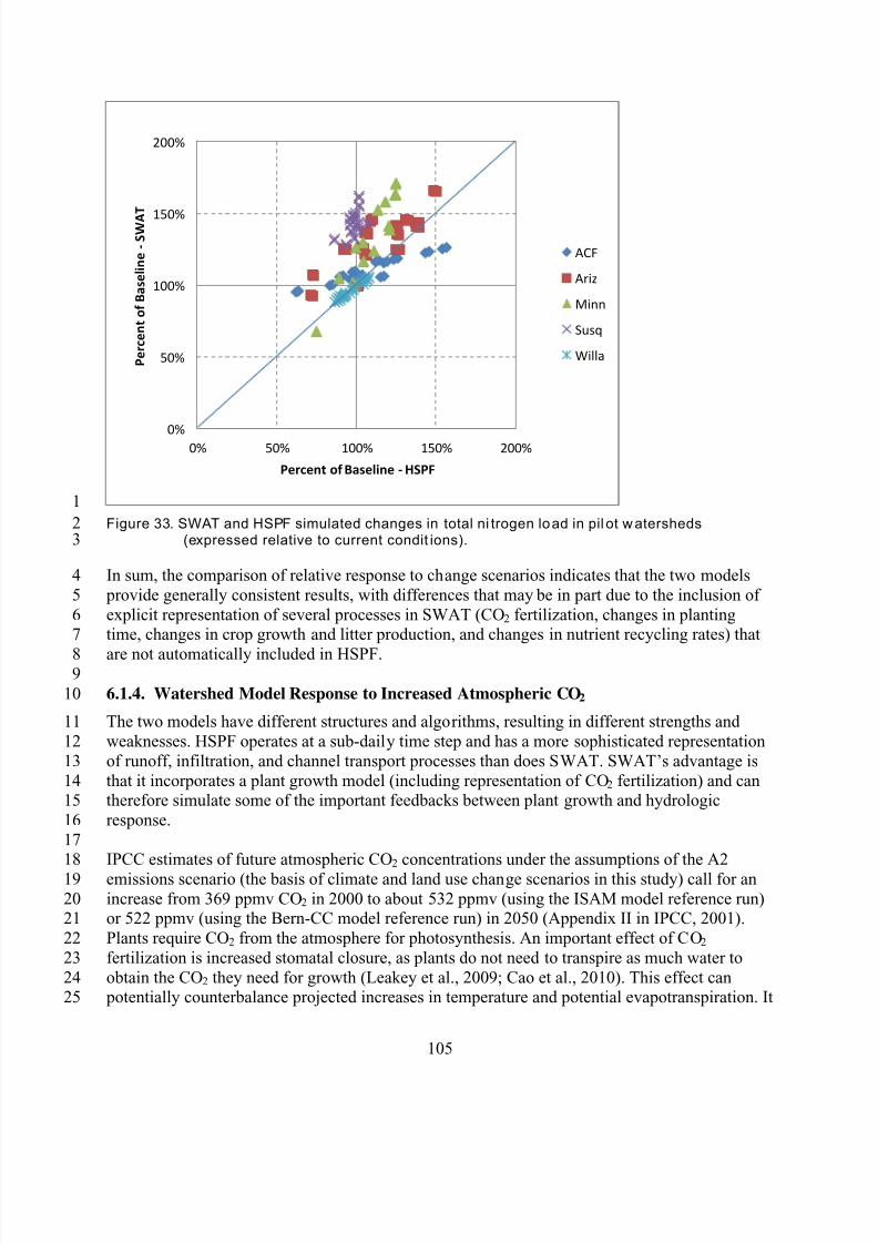
8/13/2019 20 Watersheds Erd
http://slidepdf.com/reader/full/20-watersheds-erd 117/186
1
23
4
5
67
89
10
11
12
13
1415
16
1718
19
2021
22
23
2425
0%
50%
100%
150%
200%
0% 50% 100% 150% 200%
P e r c e n t o f B a s e l i n e - S W A
T
Percent of Baseline - HSPF
ACF
Ariz
Minn
Susq
Willa
Figure 33. SWAT and HSPF simulated changes in total ni trogen load in pil ot watersheds (expressed relative to current condit ions).
In sum, the comparison of relative response to change scenarios indicates that the two models
provide generally consistent results, with differences that may be in part due to the inclusion of
explicit representation of several processes in SWAT (CO2 fertilization, changes in plantingtime, changes in crop growth and litter production, and changes in nutrient recycling rates) that
are not automatically included in HSPF.
6.1.4. Watershed Model Response to Increased Atmospheric CO2
The two models have different structures and algorithms, resulting in different strengths and
weaknesses. HSPF operates at a sub-daily time step and has a more sophisticated representation
of runoff, infiltration, and channel transport processes than does SWAT. SWAT’s advantage is
that it incorporates a plant growth model (including representation of CO2 fertilization) and cantherefore simulate some of the important feedbacks between plant growth and hydrologic
response.
IPCC estimates of future atmospheric CO2 concentrations under the assumptions of the A2
emissions scenario (the basis of climate and land use change scenarios in this study) call for an
increase from 369 ppmv CO2 in 2000 to about 532 ppmv (using the ISAM model reference run)or 522 ppmv (using the Bern-CC model reference run) in 2050 (Appendix II in IPCC, 2001).
Plants require CO2 from the atmosphere for photosynthesis. An important effect of CO2
fertilization is increased stomatal closure, as plants do not need to transpire as much water to
obtain the CO2 they need for growth (Leakey et al., 2009; Cao et al., 2010). This effect can potentially counterbalance projected increases in temperature and potential evapotranspiration. It
105
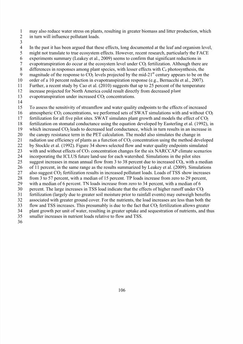
8/13/2019 20 Watersheds Erd
http://slidepdf.com/reader/full/20-watersheds-erd 118/186
1
2
34
5
67
8
9
1011
12
1314
15
16
1718
19
2021
22
2324
25
2627
28
2930
31
32
3334
35
36
may also reduce water stress on plants, resulting in greater biomass and litter production, which
in turn will influence pollutant loads.
In the past it has been argued that these effects, long documented at the leaf and organism level,
might not translate to true ecosystem effects. However, recent research, particularly the FACE
experiments summary (Leakey et al., 2009) seems to confirm that significant reductions inevapotranspiration do occur at the ecosystem level under CO2 fertilization. Although there are
differences in responses among plant species, with lesser effects with C4 photosynthesis, the
magnitude of the response to CO2 levels projected by the mid-21st century appears to be on the
order of a 10 percent reduction in evapotranspiration response (e.g., Bernacchi et al., 2007).Further, a recent study by Cao et al. (2010) suggests that up to 25 percent of the temperature
increase projected for North America could result directly from decreased plant
evapotranspiration under increased CO2 concentrations.
To assess the sensitivity of streamflow and water quality endpoints to the effects of increased
atmospheric CO2 concentrations, we performed sets of SWAT simulations with and without CO2
fertilization for all five pilot sites. SWAT simulates plant growth and models the effect of CO2fertilization on stomatal conductance using the equation developed by Easterling et al. (1992), in
which increased CO2 leads to decreased leaf conductance, which in turn results in an increase in
the canopy resistance term in the PET calculation. The model also simulates the change inradiation use efficiency of plants as a function of CO2 concentration using the method developed
by Stockle et al. (1992). Figure 34 shows selected flow and water quality endpoints simulated
with and without effects of CO2 concentration changes for the six NARCCAP climate scenariosincorporating the ICLUS future land-use for each watershed. Simulations in the pilot sites
suggest increases in mean annual flow from 3 to 38 percent due to increased CO2, with a median
of 11 percent, in the same range as the results summarized by Leakey et al. (2009). Simulationsalso suggest CO2 fertilization results in increased pollutant loads. Loads of TSS show increases
from 3 to 57 percent, with a median of 15 percent. TP loads increase from zero to 29 percent,
with a median of 6 percent. TN loads increase from zero to 34 percent, with a median of 6 percent. The large increases in TSS load indicate that the effects of higher runoff under CO2
fertilization (largely due to greater soil moisture prior to rainfall events) may outweigh benefits
associated with greater ground cover. For the nutrients, the load increases are less than both the
flow and TSS increases. This presumably is due to the fact that CO2 fertilization allows greater plant growth per unit of water, resulting in greater uptake and sequestration of nutrients, and thus
smaller increases in nutrient loads relative to flow and TSS.
106
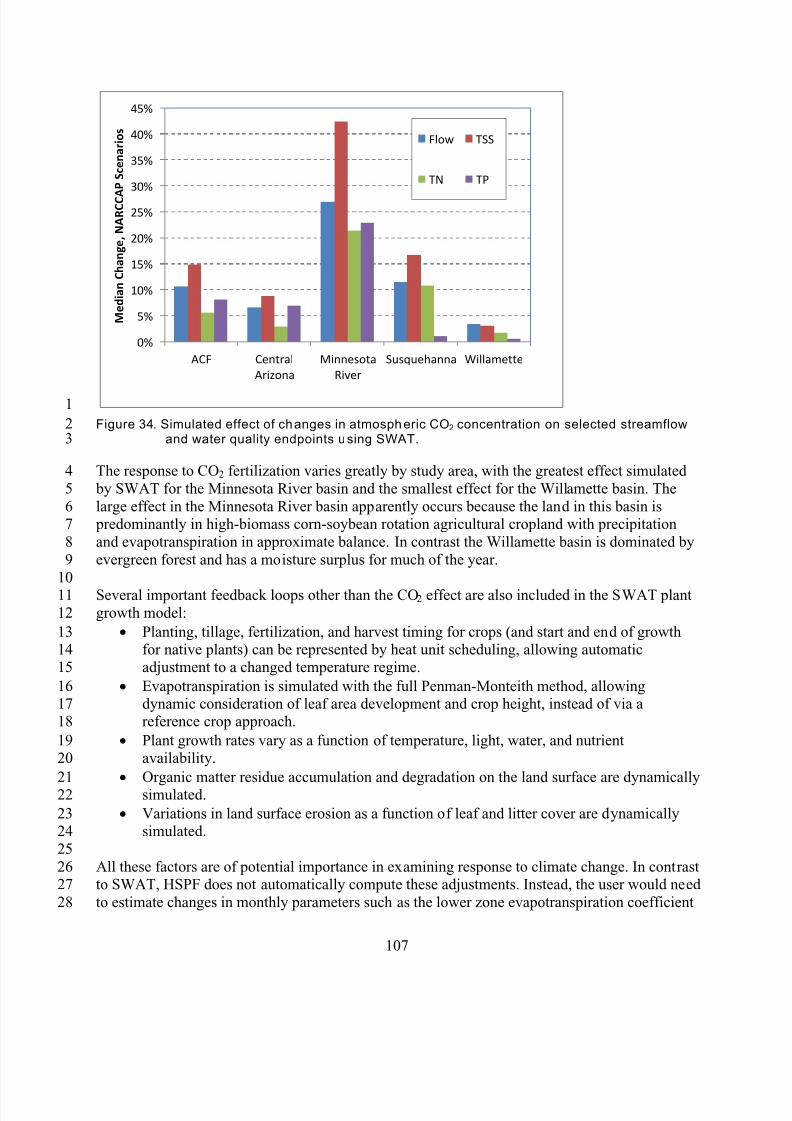
8/13/2019 20 Watersheds Erd
http://slidepdf.com/reader/full/20-watersheds-erd 119/186
1
23
4
5
67
8
9
10
1112
131415
161718
1920
2122
2324
25
2627
28
0%
5%
10%
15%
20%
25%
30%
35%
40%
45%
ACF Central
Arizona
Minnesota
River
Susquehanna Willamette
M e d i a n C h a n g e ,
N A R C C A
P S c e n a r i o s
Flow TSS
TN TP
Figure 34. Simulated effect of changes in atmospheric CO2 concentration on selected streamflowand water quality endpoints using SWAT.
The response to CO2 fertilization varies greatly by study area, with the greatest effect simulated
by SWAT for the Minnesota River basin and the smallest effect for the Willamette basin. The
large effect in the Minnesota River basin apparently occurs because the land in this basin is predominantly in high-biomass corn-soybean rotation agricultural cropland with precipitation
and evapotranspiration in approximate balance. In contrast the Willamette basin is dominated by
evergreen forest and has a moisture surplus for much of the year.
Several important feedback loops other than the CO2 effect are also included in the SWAT plantgrowth model:
• Planting, tillage, fertilization, and harvest timing for crops (and start and end of growthfor native plants) can be represented by heat unit scheduling, allowing automaticadjustment to a changed temperature regime.
• Evapotranspiration is simulated with the full Penman-Monteith method, allowingdynamic consideration of leaf area development and crop height, instead of via areference crop approach.
• Plant growth rates vary as a function of temperature, light, water, and nutrientavailability.
• Organic matter residue accumulation and degradation on the land surface are dynamicallysimulated.
• Variations in land surface erosion as a function of leaf and litter cover are dynamicallysimulated.
All these factors are of potential importance in examining response to climate change. In contrastto SWAT, HSPF does not automatically compute these adjustments. Instead, the user would need
to estimate changes in monthly parameters such as the lower zone evapotranspiration coefficient
107
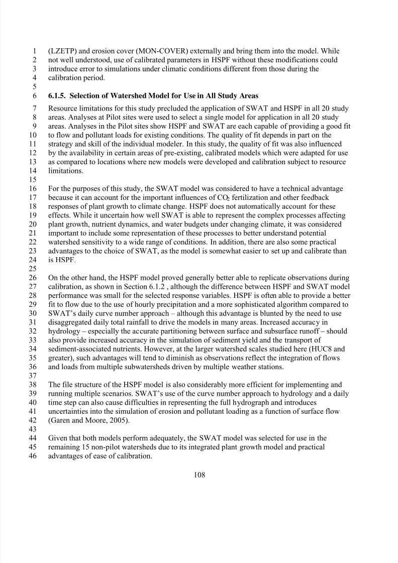
8/13/2019 20 Watersheds Erd
http://slidepdf.com/reader/full/20-watersheds-erd 120/186
1
2
34
5
678
9
1011
12
13
1415
16
1718
19
2021
22
23
2425
26
27
2829
3031
32
3334
35
36
3738
394041
42
4344
45
46
(LZETP) and erosion cover (MON-COVER) externally and bring them into the model. While
not well understood, use of calibrated parameters in HSPF without these modifications could
introduce error to simulations under climatic conditions different from those during thecalibration period.
6.1.5. Selection of Watershed Model for Use in All Study AreasResource limitations for this study precluded the application of SWAT and HSPF in all 20 studyareas. Analyses at Pilot sites were used to select a single model for application in all 20 study
areas. Analyses in the Pilot sites show HSPF and SWAT are each capable of providing a good fit
to flow and pollutant loads for existing conditions. The quality of fit depends in part on thestrategy and skill of the individual modeler. In this study, the quality of fit was also influenced
by the availability in certain areas of pre-existing, calibrated models which were adapted for use
as compared to locations where new models were developed and calibration subject to resource
limitations.
For the purposes of this study, the SWAT model was considered to have a technical advantage
because it can account for the important influences of CO2 fertilization and other feedbackresponses of plant growth to climate change. HSPF does not automatically account for these
effects. While it uncertain how well SWAT is able to represent the complex processes affecting
plant growth, nutrient dynamics, and water budgets under changing climate, it was consideredimportant to include some representation of these processes to better understand potential
watershed sensitivity to a wide range of conditions. In addition, there are also some practical
advantages to the choice of SWAT, as the model is somewhat easier to set up and calibrate than
is HSPF.
On the other hand, the HSPF model proved generally better able to replicate observations during
calibration, as shown in Section 6.1.2 , although the difference between HSPF and SWAT model
performance was small for the selected response variables. HSPF is often able to provide a betterfit to flow due to the use of hourly precipitation and a more sophisticated algorithm compared to
SWAT’s daily curve number approach – although this advantage is blunted by the need to usedisaggregated daily total rainfall to drive the models in many areas. Increased accuracy in
hydrology – especially the accurate partitioning between surface and subsurface runoff – should
also provide increased accuracy in the simulation of sediment yield and the transport ofsediment-associated nutrients. However, at the larger watershed scales studied here (HUC8 and
greater), such advantages will tend to diminish as observations reflect the integration of flows
and loads from multiple subwatersheds driven by multiple weather stations.
The file structure of the HSPF model is also considerably more efficient for implementing and
running multiple scenarios. SWAT’s use of the curve number approach to hydrology and a dailytime step can also cause difficulties in representing the full hydrograph and introducesuncertainties into the simulation of erosion and pollutant loading as a function of surface flow
(Garen and Moore, 2005).
Given that both models perform adequately, the SWAT model was selected for use in the
remaining 15 non-pilot watersheds due to its integrated plant growth model and practical
advantages of ease of calibration.
108
8/13/2019 20 Watersheds Erd
http://slidepdf.com/reader/full/20-watersheds-erd 121/186
1
2
34
5
67
8
910
11
12
13
1415
16
1718
19
2021
22
23
2425
26
27
2829
30
3132
33
3435
36
3738
3940
4142
4344
45
It should be recognized that there are other feedback cycles that are not incorporated in either
model, such as the potential for any increased rate of catastrophic forest fires (Westerling et al.,2006), changes to vegetative communities as a result of pests and disease (Berg et al., 2006), and
human adaptations such as shifts to different crops and agricultural management strategies
(Polsky and Easterling, 2001).
6.2. EFFECTS OF DIFFERENT METHODS OF DOWNSCALING OF CLIMATE
CHANGE PROJECTIONS
In general, the different climate scenarios provide a consistent picture of temperature increases
by mid-century (on the order of 2 to 3 °C), although there do appear to be systematic differences
between the scenarios (for example, the NARCCAP scenario using the GFDL model downscaledwith RCM3 typically is the coolest scenario for the watersheds studied here). In contrast,
changes in precipitation between the historical and future simulations differ widely across
models, with some producing increases and some suggesting decreases in total precipitation.
In addition, as is evident from the detailed results presented in Section Appendix X, not only the
selection of the underlying GCM, but also the choice of downscaling method, have a significantinfluence on the flow and water quality simulations. Indeed, in some basins (e.g., Minnesota
River, ACF) the difference among watershed model simulations as driven by the six NARCCAP
dynamically downscaled scenarios appears to be noticeably greater than the range of model
predictions driven by BCSD statistically downscaled or raw GCM meteorology. This leads to thesomewhat counter-intuitive observation that incorporating additional information, either from
dynamic RCMs or via statistical methods, can actually increase the perceived level of uncertainty
regarding climate change impacts – or, perhaps more accurately, provides a more realistic picture
of the uncertainty in future climate impacts.
6.2.1. “Degraded” NARCCAP Climate Scenarios
To provide a consistent basis for comparison that focuses on the differences between climatemodel outputs rather than differences in post-processing, all scenarios were adjusted to a
common minimum basis. Specifically, the raw GCM and BCSD climate products used in this
study provide only precipitation volume and air temperature and do not include explicitinformation on potential changes in the intensity of precipitation events. The following steps
were taken to develop a consistent set of climate scenario input series that differ only in the
underlying climate model and downscaling technique:
• Representation of intensification in each of the NARCCAP dynamically downscaledscenarios was based on Approach 2 in Section 5.1.4.2, which assumes that all increases in
precipitation occur in the top 30 percent of events, rather than using the direct analysis ofintensity changes provided by NARCCAP.
• Complete information on changes in weather generator statistics for dew pointtemperature, solar radiation, and wind speed was removed for the NARCCAP
dynamically downscaled scenarios, consistent with the information available for the
109
8/13/2019 20 Watersheds Erd
http://slidepdf.com/reader/full/20-watersheds-erd 122/186
1
2
3
4
5
67
89
10
1112
13
1415
16
171819
20
2122
23
2425
2627
BCSD scenarios. Incomplete information on these variables provided by the non
downscaled GCMs was also removed. (For the raw GCMs this affects weather scenarios
7, 9, and 10 – see Table 15 above).
• Penman-Monteith PET was recalculated with the revised set of climate variables.
• Simulations use current land use to remove land use change effects.
Note that these simplified or “degraded” scenarios are used only for the comparisons presented
in this section. Results presented in subsequent sections use the scenarios that contain allavailable meteorological information.
Comparison of the PET series generated with full climatological data to the degraded series inwhich only precipitation and temperature are updated shows the importance of including these
additional variables. Further, the effect of individual meteorological time series is discernible
because the original set lacked solar radiation for Scenario 5, dewpoint temperature for Scenario9, and wind speed for Scenario 10 (see Table 14). Dewpoint temperature (which tends to
increase in future, warmer climates) has the biggest impact. Including climate model-simulated
dewpoint that is consistent with the scenario temperature and precipitation regime results in areduction in estimated annual PET of about 11 percent across all the meteorological stations usedfor the five pilot watersheds. The effect appears to be greater at higher latitudes. The reduction in
PET from including simulated dewpoint is around 10 - 20 percent for the Minnesota, New York,
Oregon, and Pennsylvania stations, but only 3 – 10 percent for the Alabama, Arizona, Florida,and Georgia stations. In contrast, for Scenario 9 (for which dewpoint temperature was not
available), the original PET series were on average 1.9 percent higher than the degraded series.
Omission of solar radiation or wind speed results from the climate scenario appears to have atmost a minor impact on the estimated PET.
Table 22. Effects of omitting simulated auxili ary meteorological time series on Penman-Monteithreference crop PET estimates for “ degraded” cl imate scenarios
110
Location Scen1 Scen2 Scen3 Scen4 Scen5 Scen6 Scen7 Scen9 Scen10
AL-4.87% -4.44% -5.21% -10.90% -5.76% -4.47% -4.89% 2.66% -7.11%
AZ-2.38% -3.01% -4.12% -3.59% -2.97% -3.08% -0.99% 2.69% -3.02%
FL-7.14% -8.48% -7.45% -16.69% -9.04% -9.02% -7.35% 2.92% -10.91%
GA-9.30% -7.21% -7.79% -18.01% -10.15% -7.27% -8.71% 1.79% -14.04%
MN-14.68% -10.30% -13.73% -10.30% -16.46% -21.16% -13.83% 1.68% -16.46%
NY-23.27% -16.99% -17.68% -20.62% -22.95% -18.30% -23.01% -1.29% -20.48%
OR-15.82% -14.28% -7.75% -12.90% -13.67% -13.29% -12.73% 0.11% -10.17%
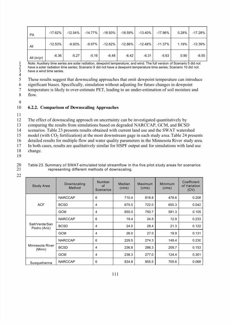
8/13/2019 20 Watersheds Erd
http://slidepdf.com/reader/full/20-watersheds-erd 123/186
PA-17.62% -12.54% -14.77% -18.93% -18.59% -13.40% -17.96% 0.28% -17.28%
All-12.53% -9.93% -9.97% -12.62% -12.86% -12.48% -11.37% 1.19% -12.39%
All (in/yr) -6.36 -5.27 -5.16 -6.48 -6.42 -6.31 -5.63 0.90 -6.55
1 Note: Auxiliary time series are solar radiation, dewpoint temperature, and wind. The full version of Scenario 5 did nothave a solar radiation time series; Scenario 9 did not have a dewpoint temperature time series; Scenario 10 did nothave a wind time series.
These results suggest that downscaling approaches that omit dewpoint temperature can introduce
significant biases. Specifically, simulation without adjusting for future changes in dewpointtemperature is likely to over-estimate PET, leading to an under-estimation of soil moisture and
flow.
6.2.2. Comparison of Downscaling Approaches
The effect of downscaling approach on uncertainty can be investigated quantitatively by
comparing the results from simulations based on degraded NARCCAP, GCM, and BCSD
scenarios. Table 23 presents results obtained with current land use and the SWAT watershedmodel (with CO2 fertilization) at the most downstream gage in each study area. Table 24 presents
detailed results for multiple flow and water quality parameters in the Minnesota River study area.
In both cases, results are qualitatively similar for HSPF output and for simulations with land usechange.
Table 23. Summary o f SWAT-simu lated total streamflow in the five pilot s tudy areas for scenarios
representing different methods of downscaling.
2345
67
8
9
10
1112
13
1415
16
1718
19
20
2122
111
Study AreaDownscaling
Method
Numberof
Scenarios
Median(cms)
Maximum(cms)
Minimum(cms)
Coefficientof Variation
(CV)
ACF
NARCCAP 6 710.4 818.8 478.6 0.208
BCSD 4 675.5 722.0 655.3 0.042
GCM 4 655.0 750.7 581.3 0.105
Salt/Verde/San
Pedro (Ariz)
NARCCAP 6 19.4 24.5 12.9 0.233
BCSD 4 24.0 28.4 21.3 0.122
GCM 4 26.0 27.0 19.9 0.131
Minnesota River(Minn)
NARCCAP 6 229.5 274.3 149.4 0.230
BCSD 4 236.8 286.3 209.7 0.153
GCM 4 238.3 277.0 124.4 0.301
Susquehanna NARCCAP 6 834.8 855.5 705.6 0.068
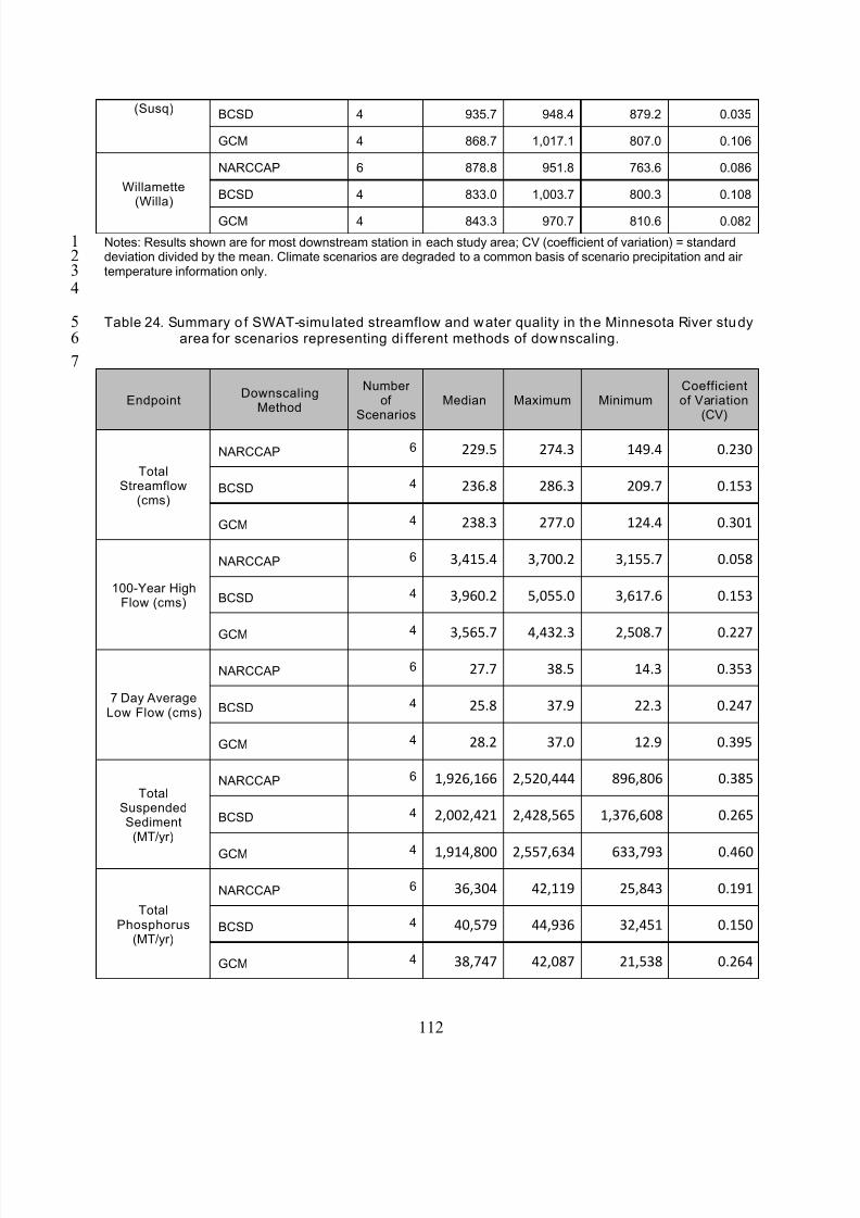
8/13/2019 20 Watersheds Erd
http://slidepdf.com/reader/full/20-watersheds-erd 124/186
(Susq) BCSD 4 935.7 948.4 879.2 0.035
GCM 4 868.7 1,017.1 807.0 0.106
NARCCAP 6 878.8 951.8 763.6 0.086
Willamette(Willa)
BCSD 4 833.0 1,003.7 800.3 0.108
GCM 4 843.3 970.7 810.6 0.082
1 Notes: Results shown are for most downstream station in each study area; CV (coefficient of variation) = standarddeviation divided by the mean. Climate scenarios are degraded to a common basis of scenario precipitation and airtemperature information only.
Table 24. Summary o f SWAT-simu lated streamflow and water quality in the Minnesota River studyarea for scenarios representing di fferent methods of downscaling.
234
56
7
112
EndpointDownscaling
Method
Numberof
ScenariosMedian Maximum Minimum
Coefficientof Variation
(CV)
TotalStreamflow
(cms)
NARCCAP 6 229.5 274.3 149.4 0.230
BCSD 4 236.8 286.3 209.7 0.153
GCM 4 238.3 277.0 124.4 0.301
100-Year HighFlow (cms)
NARCCAP 6 3,415.4 3,700.2 3,155.7 0.058
BCSD 4 3,960.2 5,055.0 3,617.6 0.153
GCM
4 3,565.7 4,432.3 2,508.7 0.227
7 Day AverageLow Flow (cms)
NARCCAP 6 27.7 38.5 14.3 0.353
BCSD 4 25.8 37.9 22.3 0.247
GCM 4 28.2 37.0 12.9 0.395
TotalSuspendedSediment
(MT/yr)
NARCCAP 6 1,926,166 2,520,444 896,806 0.385
BCSD 4 2,002,421 2,428,565 1,376,608 0.265
GCM 4 1,914,800 2,557,634 633,793 0.460
TotalPhosphorus
(MT/yr)
NARCCAP 6 36,304 42,119 25,843 0.191
BCSD 4 40,579 44,936 32,451 0.150
GCM 4 38,747 42,087 21,538 0.264
8/13/2019 20 Watersheds Erd
http://slidepdf.com/reader/full/20-watersheds-erd 125/186
Total Nitrogen(MT/yr)
NARCCAP 6 2,700 3,283 2,007 0.194
BCSD 4 3,073 3,453 2,356 0.183
GCM 4 2,889 3,162 1,489 0.292
5
10
15
20
25
30
1 Notes: Results shown are for most downstream station in each study area; CV (coefficient of variation) = standarddeviation divided by the mean. Climate scenarios are degraded to a common basis of scenario precipitation and airtemperature information only.
Results show considerable variability among climate models and downscaling techniques indifferent basins and for different streamflow and water quality endpoints. No consistent pattern
attributable to downscaling method is evident for the case where all climate model outputs are
degraded to a common basis of precipitation and air temperature only, As was discussed inSection 6.1.4. the additional information on other meteorological variables can have a profound
effect on PET and watershed responses.
It is noteworthy that the dynamically downscaled results may differ significantly from thestatistically downscaled results from the same GCM, and that the results may also be quite
different when the same GCM is downscaled with a different RCM (e.g., compare scenarios W1
and W5 for CGCM3, also W3 and W4 for the GFDL). As noted in Section 5.1.2. , directcomparison between NARCCAP and BCSD downscaling of a single GCM can only be reliably
undertaken for the GFDL and CGCM3 models, as slightly different GCM runs were used to
produce NARCCAP and BCSD results for other GCMs.
Both the GFDL and CGCM3 A2 scenario runs for 2041-2070 were downscaled with two
different NARCCAP RCMs - with one RCM (RCM3) in common between the two. A
comparison in terms of the ratio of simulated future mean annual flow to simulated current meanannual flow, using SWAT, is made in Figure 35 for the GFDL and in Figure 36 for the CGCM3
model. For both GCMs, the NARCCAP downscaling, BCSD downscaling, and raw GCM output
produce relatively consistent results for the Willamette and Susquehanna basins, but diverge forthe Minnesota River. For the Arizona basin, the two different downscaling approaches diverge
for the GFDL but not the CGCM3 GCM. Elevated CVs on mean annual flow in both the
Minnesota River and Arizona basins appear to be largely due to the difference in downscalingresults obtained with the GFDL high-resolution regional model, which suggests lower flow than
other dynamically downscaled interpretations of the GFDL GCM.
234
6
7
89
11
1213
14
16
17
1819
21
2223
24
26
27
2829
31
113
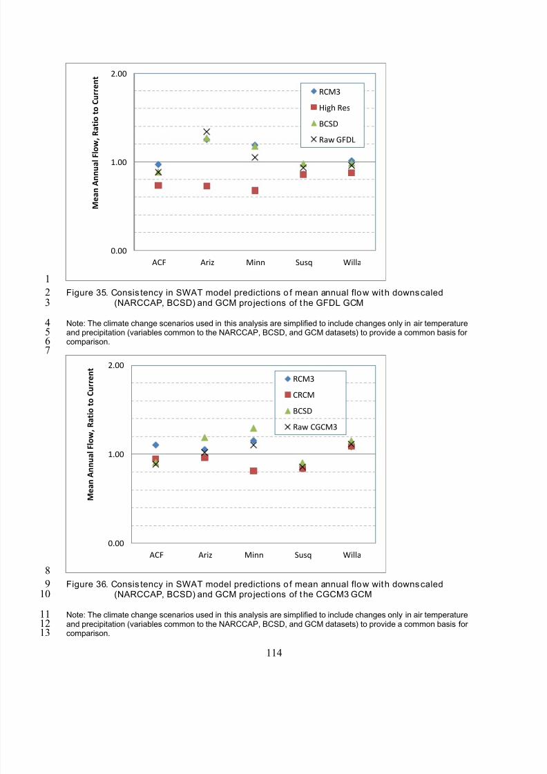
8/13/2019 20 Watersheds Erd
http://slidepdf.com/reader/full/20-watersheds-erd 126/186
0.00
1.00
2.00
ACF Ariz Minn Susq Willa
M e a n A n n u a l F l o w , R
a t i o t o C u r r e n t
RCM3
High Res
BCSD
Raw GFDL
1
2 Figure 35. Consis tency in SWAT model predictions o f mean annual flow with downscaled(NARCCAP, BCSD) and GCM pro jections of t he GFDL GCM
Note: The climate change scenarios used in this analysis are simplified to include changes only in air temperatureand precipitation (variables common to the NARCCAP, BCSD, and GCM datasets) to provide a common basis forcomparison.
3
4567
8
910
2.00
M e a n A n n u a l F l o w ,
R a t i o t o C u r r e n t
1.00
RCM3
CRCM
BCSD
Raw CGCM3
0.00ACF Ariz Minn Susq Willa
Figure 36. Consis tency in SWAT model predictions o f mean annual flow with downscaled(NARCCAP, BCSD) and GCM pro jections of t he CGCM3 GCM
Note: The climate change scenarios used in this analysis are simplified to include changes only in air temperatureand precipitation (variables common to the NARCCAP, BCSD, and GCM datasets) to provide a common basis forcomparison.
111213
114
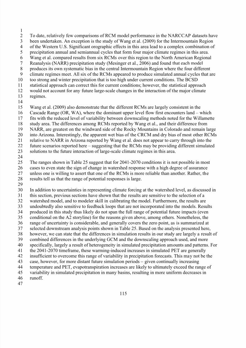
8/13/2019 20 Watersheds Erd
http://slidepdf.com/reader/full/20-watersheds-erd 127/186
12
3
45
6
7
89
10
1112
13
1415
16
17
1819
20
2122
23
2425
26
2728
2930
3132
33
3435
36
3738
39
404142
43
4445
46
47
To date, relatively few comparisons of RCM model performance in the NARCCAP datasets have
been undertaken. An exception is the study of Wang et al. (2009) for the Intermountain Region
of the Western U.S. Significant orographic effects in this area lead to a complex combination of precipitation annual and semiannual cycles that form four major climate regimes in this area.
Wang et al. compared results from six RCMs over this region to the North American Regional
Reanalysis (NARR) precipitation study (Mesinger et al., 2006) and found that each model
produces its own systematic bias in the central Intermountain Region where the four differentclimate regimes meet. All six of the RCMs appeared to produce simulated annual cycles that are
too strong and winter precipitation that is too high under current conditions. The BCSD
statistical approach can correct this for current conditions; however, the statistical approachwould not account for any future large-scale changes in the interaction of the major climate
regimes.
Wang et al. (2009) also demonstrate that the different RCMs are largely consistent in the
Cascade Range (OR, WA), where the dominant upper level flow first encounters land – which
fits with the reduced level of variability between downscaling methods noted for the Willamette
study area. The differences among RCMs reported by Wang et al., and their difference from NARR, are greatest on the windward side of the Rocky Mountains in Colorado and remain large
into Arizona. Interestingly, the apparent wet bias of the CRCM and dry bias of most other RCMs
relative to NARR in Arizona reported by Wang et al. does not appear to carry through into thefuture scenarios reported here – suggesting that the RCMs may be providing different simulated
solutions to the future interaction of large-scale climate regimes in this area.
The ranges shown in Table 25 suggest that for 2041-2070 conditions it is not possible in most
cases to even state the sign of change in watershed response with a high degree of assurance
unless one is willing to assert that one of the RCMs is more reliable than another. Rather, theresults tell us that the range of potential responses is large.
In addition to uncertainties in representing climate forcing at the watershed level, as discussed in
this section, previous sections have shown that the results are sensitive to the selection of awatershed model, and to modeler skill in calibrating the model. Furthermore, the results are
undoubtedly also sensitive to feedback loops that are not incorporated into the models. Results
produced in this study thus likely do not span the full range of potential future impacts (evenconditional on the A2 storyline) for the reasons given above, among others. Nonetheless, the
range of uncertainty is considerable, and generally covers the zero point, as is summarized at
selected downstream analysis points shown in Table 25. Based on the analysis presented here,however, we can state that the differences in simulation results in our study are largely a result of
combined differences in the underlying GCM and the downscaling approach used, and more
specifically, largely a result of heterogeneity in simulated precipitation amounts and patterns. Forthe 2041-2070 timeframe, these warming-induced increases in simulated PET are generallyinsufficient to overcome this range of variability in precipitation forecasts. This may not be the
case, however, for more distant future simulation periods – given continually increasing
temperature and PET, evapotranspiration increases are likely to ultimately exceed the range ofvariability in simulated precipitation in many basins, resulting in more uniform decreases in
runoff.
115
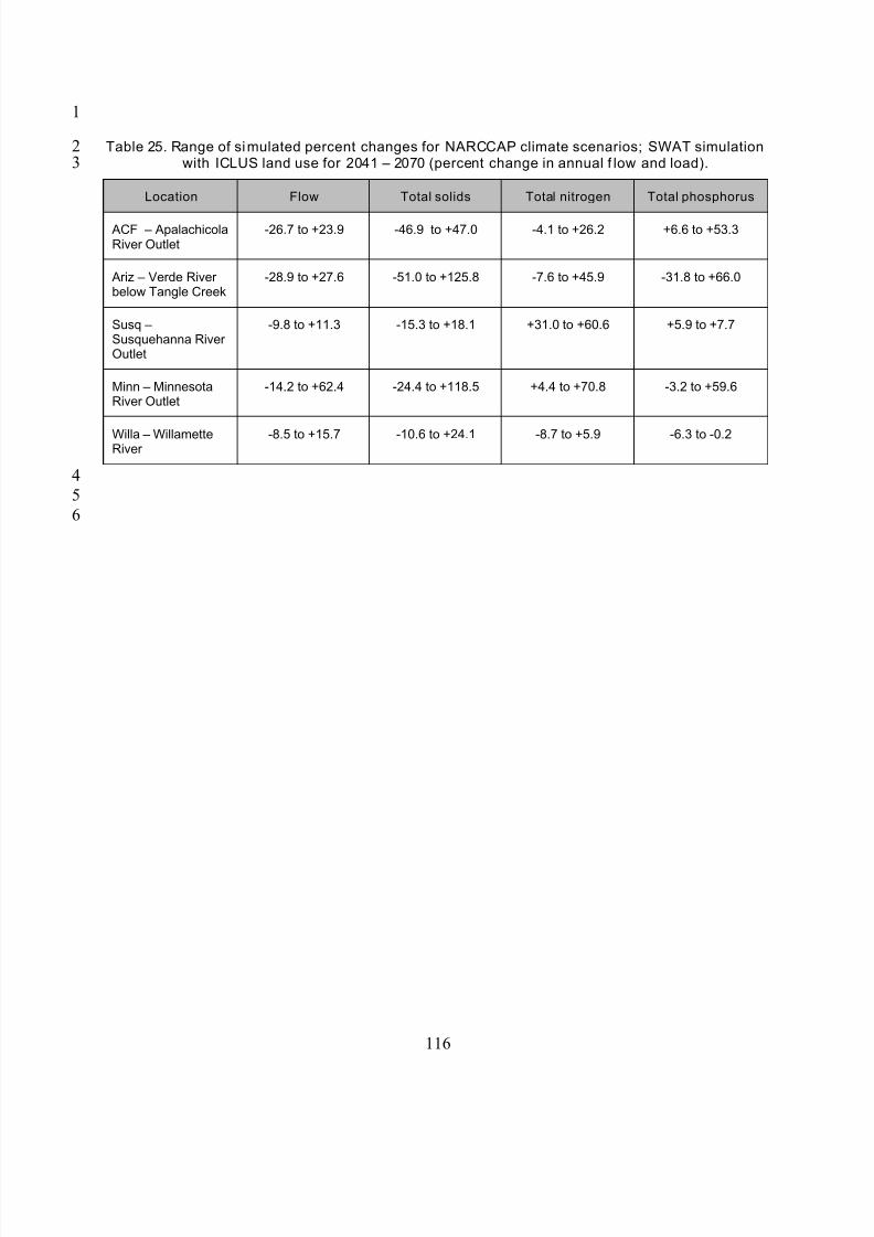
8/13/2019 20 Watersheds Erd
http://slidepdf.com/reader/full/20-watersheds-erd 128/186
1
23
4
5
6
Table 25. Range of simulated percent changes for NARCCAP climate scenarios; SWAT simulationwith ICLUS land use for 2041 – 2070 (percent change in annual f low and load).
Location Flow Total solids Total nitrogen Total phosphorus
ACF – ApalachicolaRiver Outlet
-26.7 to +23.9 -46.9 to +47.0 -4.1 to +26.2 +6.6 to +53.3
Ariz – Verde Riverbelow Tangle Creek
-28.9 to +27.6 -51.0 to +125.8 -7.6 to +45.9 -31.8 to +66.0
Susq –Susquehanna RiverOutlet
-9.8 to +11.3 -15.3 to +18.1 +31.0 to +60.6 +5.9 to +7.7
Minn – MinnesotaRiver Outlet
-14.2 to +62.4 -24.4 to +118.5 +4.4 to +70.8 -3.2 to +59.6
Willa – WillametteRiver
-8.5 to +15.7 -10.6 to +24.1 -8.7 to +5.9 -6.3 to -0.2
116
8/13/2019 20 Watersheds Erd
http://slidepdf.com/reader/full/20-watersheds-erd 129/186
1 7. RESULTS IN ALL 20 WATERSHEDS: REGIONAL SENSITIVITY TO CLIMATE
CHANGE AND URBAN DEVELOPMENT
This section provides a summary of SWAT simulation results for all 20 watersheds. Tabularresults are presented for a single representative analysis point in each study area (Table 26). For
study areas composed of a single watershed, this is the outlet (pour point) of the entire study
area. For study areas composed of multiple, adjacent watersheds draining to the coast, theanalysis point reported here is at or near the outlet of the largest river within the study area.
Graphical results for key indicators are shown for all HUC8s contained within the 20 watersheds
in Section 7. More detailed scenario results including results at multiple stations within eachstudy area are reported in Appendix X for the 5 pilot sites and Appendix Y for all other sites.
The comparison uses baseline climate and land use with the six mid-21st
century NARCCAP
climate change scenarios, and the 2050 ICLUS urban and residential development scenario.Scenarios also assumed future increases in atmospheric CO2.
Table 26. Downs tream stations where simulation results are presented.
2
34
5
67
8
910
11
12
131415
16
Study Area Location Reporting Results
Apalachicola-Chattahoochee-Flint(ACF) Basins
Apalachicola R at outlet
Coastal Southern California Los Angeles R at outlet
Cook Inlet Basin Kenai R at Soldotna
Georgia-Florida Coastal Plain Suwanee R at outlet
Illinois River Basin Illinois R at Marseilles, IL
Lake Erie-Lake St. Clair Drainages Maumee R at outlet
Lake Pontchartrain Drainage Amite R at outlet
Loup/Elkhorn River Basin Elkhorn R at outlet
Minnesota River Basin Minnesota R at outlet
Neuse/Tar River Basins Neuse R at outlet
New England Coastal Basins Merrimack R at outlet
Powder/Tongue River Basin Tongue R at outlet
Rio Grande Valley Rio Grande R below Albuquerque
Sacramento River Basin Sacramento R at outlet
Salt, Verde, and San Pedro RiverBasins
Salt River nr Roosevelt
South Platte River Basin S. Platte R at outlet
Susquehanna River Basin Susquehanna R at outlet
Trinity River Basin Trinity R at outlet
Upper Colorado River Basin Colorado R nr State Line
Willamette River Basin Willamette R at outlet
17
18
117
8/13/2019 20 Watersheds Erd
http://slidepdf.com/reader/full/20-watersheds-erd 130/186
1
2
3
45
678
9
1011
12
13
1415
16
1718
19
2021
22
23
2425
26
27
2829
3031
32
3334
35
36
3738
7.1. SENSITIVITY TO CLIMATE CHANGE SCENARIOS
Results across all watersheds for scenarios involving only climate change (that is, with land use
held constant at existing conditions) are shown in this section. For endpoints other than days to
flow centroid the results are shown as a percentage relative to the current baseline (generally,1972-2003), allowing comparison across multiple basins with different magnitudes of flows and
pollutant loads. The six NARCCAP dynamically downscaled climate scenarios are shown incolumns, while the last column gives the median of the six NARCCAP scenarios at the selectedanalysis point. For Cook Inlet (Alaska) results are shown only for the three NARCCAP scenarios
that provide climate projections for this portion of Alaska.
Table 27 summarizes results for total average annual flow volume, with results ranging from
63% to 240% of current average flows. Results for 7-day low flows and 100-year peak flows
(estimated with log-Pearson III fit) are shown in Table 28 and Table 29, respectively. The Kenai
River has by far the greatest increase in 7-day low flows because warmer temperatures alter thesnow/ice melt regime, while the largest increases in 100-year peak flows are for the Neuse River
on the east coast.
Table 30 summarizes the estimated change in days to flow centroid relative to the start of the
water year. Many stations show negative shifts, indicating earlier snowmelt resulting in an earlier
center of flow mass. In contrast, several stations show positive shifts due to increased summer precipitation.
Results for the Richards-Baker flashiness index (Table 31) show generally small percentage
changes, with a few exceptions. Baker et al. (2004) suggest that changes on the order of 10 percent or more may be statistically significant. It is likely, however, that the focus on larger
watersheds reduces the observed flashiness response.
Simulated changes in pollutant loads (TSS, TP, TN) are summarized in Table 34. The patternsare generally similar to changes in flow. Increases in pollutant loads are suggested for many
watersheds, but there are also basins where loads decline, mostly due to reduced flows.
For most measures in most watersheds, there is a substantial amount of variability between
predictions based on different downscaled climate products. This reflects our uncertainty in predicting future climate, especially the future joint distribution of precipitation and potential
evapotranspiration that is fundamental to watershed response, and reinforces the need for an
ensemble approach for evaluating the range of potential responses.
118
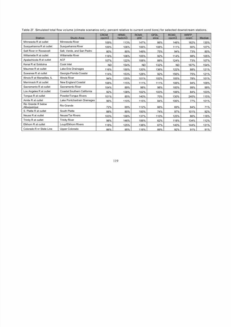
8/13/2019 20 Watersheds Erd
http://slidepdf.com/reader/full/20-watersheds-erd 131/186
119
Table 27. Simulated total flow vo lume (climate scenarios onl y; percent relative to current condi tions) for selected downst ream stations.
CRCM_ HRM3_ RCM3_ GFDL_ RCM3_ WRFP_Station Study Area cgcm3 hadcm3 gfdl slice cgcm3 ccsm Median
Minnesota R at outlet Minnesota River 109% 113% 147% 86% 146% 162% 130%
Susquehanna R at outlet Susquehanna River 109% 106% 106% 108% 111% 90% 107%
Salt River nr Roosevelt Salt, Verde, and San Pedro 80% 80% 149% 75% 94% 73% 80%
Willamette R at outlet Willamette River116% 106% 105% 92% 114% 98% 105%
Apalachicola R at outlet ACF 107% 122% 108% 88% 124% 73% 107%
Kenai R at Soldotna Cook Inlet ND 154% ND 132% ND 167% 154%
Maumee R at outlet Lake Erie Drainages 116% 150% 120% 136% 122% 88% 121%
Suwanee R at outlet Georgia-Florida Coastal 114% 153% 128% 92% 156% 75% 121%
Illinois R at Marseilles, IL Illinois River 94% 125% 101% 102% 105% 78% 101%
Merrimack R at outlet New England Coastal 108% 115% 111% 111% 106% 94% 109%
Sacramento R at outlet Sacramento River 104% 89% 98% 98% 100% 99% 99%
Los Angeles R at outlet Coastal Southern California 92% 138% 102% 103% 106% 84% 103%
Tongue R at outlet Powder/Tongue Rivers 101% 85% 140% 70% 130% 240% 115%
Amite R at outlet Lake Pontchartrain Drainages 96% 110% 115% 84% 106% 77% 101%
Rio Grande R below Albuquerque
Rio Grande72% 69% 112% 66% 69% 84% 71%
S. Platte R at outlet South Platte 88% 80% 100% 74% 97% 101% 92%
Neuse R at outlet Neuse/Tar Rivers 103% 158% 137% 110% 125% 86% 118%
Trinity R at outlet Trinity River 98% 146% 106% 62% 118% 134% 112%
Elkhorn R at outlet Loup/Elkhorn Rivers 118% 125% 138% 67% 140% 144% 131%
Colorado R nr State Line Upper Colorado 86% 95% 116% 89% 92% 91% 91%
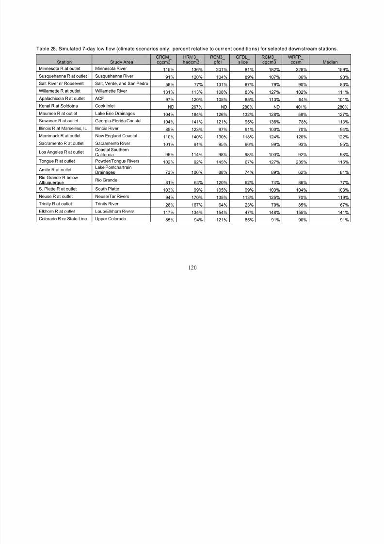
8/13/2019 20 Watersheds Erd
http://slidepdf.com/reader/full/20-watersheds-erd 132/186
Table 28. Simulated 7-day low flow (climate scenarios only; percent relative to current conditio ns) for selected down stream stations.
Station Study AreaCRCM_ HRM3_ RCM3_ GFDL_ RCM3_ WRFP_
Mediancgcm3 hadcm3 gfdl slice cgcm3 ccsm
Minnesota R at outlet Minnesota River 115% 136% 201% 81% 182% 228% 159%
Susquehanna R at outlet Susquehanna River 91% 120% 104% 89% 107% 86% 98%
Salt River nr Roosevelt Salt, Verde, and San Pedro 58% 77% 131% 87% 79% 90% 83%
Willamette R at outlet Willamette River 131% 113% 108% 83% 127% 102% 111%
Apalachicola R at outlet ACF 97% 120% 105% 85% 113% 64% 101%
Kenai R at Soldotna Cook Inlet ND 267% ND 280% ND 401% 280%
Maumee R at outlet Lake Erie Drainages 104% 184% 126% 132% 128% 58% 127%
Suwanee R at outlet Georgia-Florida Coastal 104% 141% 121% 95% 136% 78% 113%
Illinois R at Marseilles, IL Illinois River 85% 123% 97% 91% 100% 70% 94%
Merrimack R at outlet New England Coastal 110% 140% 130% 118% 124% 120% 122%
Sacramento R at outlet Sacramento River 101% 91% 95% 96% 99% 93% 95%
Los Angeles R at outletCoastal SouthernCalifornia 96% 114% 98% 98% 100% 92% 98%
Tongue R at outlet Powder/Tongue Rivers 102% 92% 145% 67% 127% 235% 115%
Amite R at outletLake PontchartrainDrainages 73% 106% 88% 74% 89% 62% 81%
Rio Grande R below Albuquerque
Rio Grande81% 64% 120% 62% 74% 86% 77%
S. Platte R at outlet South Platte 103% 99% 105% 99% 103% 104% 103%Neuse R at outlet Neuse/Tar Rivers 94% 170% 135% 113% 125% 70% 119%
Trinity R at outlet Trinity River 26% 167% 64% 23% 70% 85% 67%
Elkhorn R at outlet Loup/Elkhorn Rivers 117% 134% 154% 47% 148% 155% 141%
Colorado R nr State Line Upper Colorado 85% 94% 121% 85% 91% 90% 91%
120
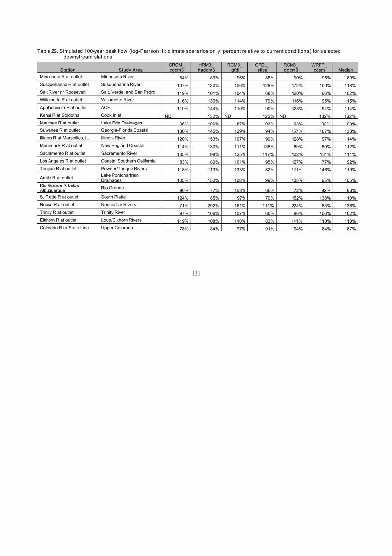
8/13/2019 20 Watersheds Erd
http://slidepdf.com/reader/full/20-watersheds-erd 133/186
Table 29. Simulated 100-year peak flow (log-Pearson III; climate scenarios onl y; percent relative to current co ndition s) for s electeddownstream stations.
Station Study AreaCRCM_ HRM3_ RCM3_ GFDL_ RCM3_ WRFP_
Mediancgcm3 hadcm3 gfdl slice c gcm3 ccsm
Minnesota R at outlet Minnesota River 84% 83% 96% 88% 90% 96% 89%
Susquehanna R at outlet Susquehanna River 107% 130% 106% 128% 172% 100% 118%
Salt River nr Roosevelt Salt, Verde, and San Pedro 119% 101% 104% 68% 120% 66% 102%
Willamette R at outlet Willamette River 116% 130% 114% 79% 116% 95% 115%
Apalachicola R at outlet ACF 119% 144% 110% 90% 128% 94% 114%
Kenai R at Soldotna Cook Inlet ND 132% ND 125% ND 132% 132%
Maumee R at outlet Lake Erie Drainages 96% 106% 87% 93% 93% 92% 93%
Suwanee R at outlet Georgia-Florida Coastal 130% 145% 129% 94% 157% 107% 130%
Illinois R at Marseilles, IL Illinois River 120% 153% 107% 99% 128% 97% 114%
Merrimack R at outlet New England Coastal 114% 130% 111% 138% 89% 80% 112%
Sacramento R at outlet Sacramento River 105% 98% 125% 117% 102% 131% 111%
Los Angeles R at outlet Coastal Southern California 83% 89% 161% 95% 127% 77% 92%
Tongue R at outlet Powder/Tongue Rivers 118% 113% 133% 82% 121% 146% 119%
Amite R at outletLake PontchartrainDrainages 105% 150% 108% 99% 105% 65% 105%
Rio Grande R below Albuquerque
Rio Grande90% 77% 108% 66% 72% 92% 83%
S. Platte R at outlet South Platte 124% 85% 97% 79% 152% 138% 110%
Neuse R at outlet Neuse/Tar Rivers 71% 292% 161% 111% 224% 63% 136%
Trinity R at outlet Trinity River 97% 106% 107% 60% 86% 106% 102%
Elkhorn R at outlet Loup/Elkhorn Rivers 119% 108% 110% 83% 141% 110% 110%
Colorado R nr State Line Upper Colorado 78% 84% 97% 91% 94% 84% 87%
121
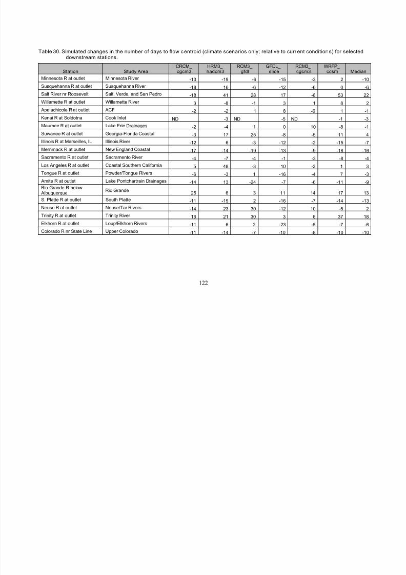
8/13/2019 20 Watersheds Erd
http://slidepdf.com/reader/full/20-watersheds-erd 134/186
Table 30. Simulated changes in the number of days to flow c entroid (climate scenarios only; relative to current condition s) for selecteddownstream stations.
CRCM_ HRM3_ RCM3_ GFDL_ RCM3_ WRFP_MedianStation Study Area cgcm3 hadcm3 gfdl slice cgcm3 ccsm
Minnesota R at outlet Minnesota River -13 -19 -6 -15 -3 2 -10
Susquehanna R at outlet Susquehanna River -18 16 -6 -12 -6 0 -6
Salt River nr Roosevelt Salt, Verde, and San Pedro -18 41 28 17 -6 53 22
Willamette R at outlet Willamette River 3 -8 -1 3 1 8 2
Apalachicola R at outlet ACF -2 -2 1 8 -6 1 -1
Kenai R at Soldotna Cook Inlet ND -3 ND -5 ND -1 -3
Maumee R at outlet Lake Erie Drainages -2 -4 1 0 10 -8 -1
Suwanee R at outlet Georgia-Florida Coastal -3 17 25 -8 -5 11 4
Illinois R at Marseilles, IL Illinois River -12 6 -3 -12 -2 -15 -7
Merrimack R at outlet New England Coastal -17 -14 -19 -13 -9 -18 -16
Sacramento R at outlet Sacramento River -4 -7 -4 -1 -3 -8 -4
Los Angeles R at outlet Coastal Southern California 5 48 -3 10 -3 1 3
Tongue R at outlet Powder/Tongue Rivers -6 -3 1 -16 -4 7 -3
Amite R at outlet Lake Pontchartrain Drainages -14 13 -24 -7 -6 -11 -9
Rio Grande R below Albuquerque
Rio Grande25 6 3 11 14 17 13
S. Platte R at outlet South Platte -11 -15 2 -16 -7 -14 -13Neuse R at outlet Neuse/Tar Rivers -14 23 30 -12 10 -5 2
Trinity R at outlet Trinity River 16 21 30 3 6 37 18
Elkhorn R at outlet Loup/Elkhorn Rivers -11 6 2 -23 -5 -7 -6
Colorado R nr State Line Upper Colorado -11 -14 -7 -10 -8 -10 -10
122
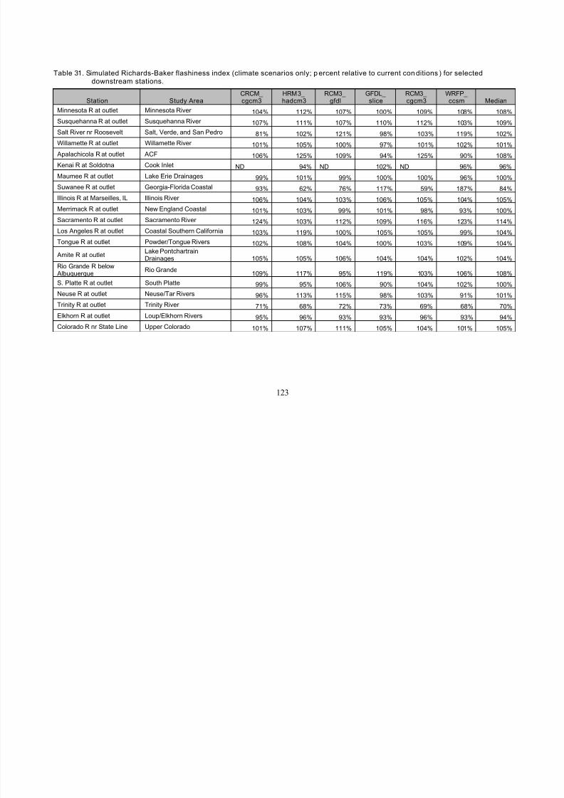
8/13/2019 20 Watersheds Erd
http://slidepdf.com/reader/full/20-watersheds-erd 135/186
Table 31. Simulated Richards-Baker flashiness index (climate scenarios only; p ercent relative to current con ditions ) for selecteddownstream stations.
Station Study AreaCRCM_ HRM3_ RCM3_ GFDL_ RCM3_ WRFP_
Mediancgcm3 hadcm3 gfdl slice cgcm3 ccsm
Minnesota R at outlet Minnesota River 104% 112% 107% 100% 109% 108% 108%
Susquehanna R at outlet Susquehanna River 107% 111% 107% 110% 112% 103% 109%
Salt River nr Roosevelt Salt, Verde, and San Pedro 81% 102% 121% 98% 103% 119% 102%
Willamette R at outlet Willamette River 101% 105% 100% 97% 101% 102% 101%
Apalachicola R at outlet ACF 106% 125% 109% 94% 125% 90% 108%
Kenai R at Soldotna Cook Inlet ND 94% ND 102% ND 96% 96%
Maumee R at outlet Lake Erie Drainages 99% 101% 99% 100% 100% 96% 100%
Suwanee R at outlet Georgia-Florida Coastal 93% 62% 76% 117% 59% 187% 84%
Illinois R at Marseilles, IL Illinois River 106% 104% 103% 106% 105% 104% 105%
Merrimack R at outlet New England Coastal 101% 103% 99% 101% 98% 93% 100%
Sacramento R at outlet Sacramento River 124% 103% 112% 109% 116% 123% 114%
Los Angeles R at outlet Coastal Southern California 103% 119% 100% 105% 105% 99% 104%
Tongue R at outlet Powder/Tongue Rivers 102% 108% 104% 100% 103% 109% 104%
Amite R at outletLake PontchartrainDrainages 105% 105% 106% 104% 104% 102% 104%
Rio Grande R below Albuquerque
Rio Grande109% 117% 95% 119% 103% 106% 108%
S. Platte R at outlet South Platte 99% 95% 106% 90% 104% 102% 100%
Neuse R at outlet Neuse/Tar Rivers 96% 113% 115% 98% 103% 91% 101%
Trinity R at outlet Trinity River 71% 68% 72% 73% 69% 68% 70%
Elkhorn R at outlet Loup/Elkhorn Rivers 95% 96% 93% 93% 96% 93% 94%
Colorado R nr State Line Upper Colorado 101% 107% 111% 105% 104% 101% 105%
123
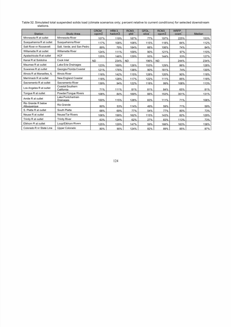
8/13/2019 20 Watersheds Erd
http://slidepdf.com/reader/full/20-watersheds-erd 136/186
Table 32. Simulated total suspended solids load (climate scenarios only; p ercent relative to current condit ions) for selected downstream
stations.
Station Study AreaCRCM_ HRM3_ RCM3_ GFDL_ RCM3_ WRFP_
Mediancgcm3 hadcm3 gfdl slice cgcm3 ccsm
Minnesota R at outlet Minnesota River 107% 119% 187% 77% 197% 225% 153%
Susquehanna R at outlet Susquehanna River 117% 108% 108% 115% 118% 84% 112%
Salt River nr Roosevelt Salt, Verde, and San Pedro 89% 79% 184% 66% 106% 74% 84%
Willamette R at outlet Willamette River 124% 111% 109% 90% 121% 97% 110%
Apalachicola R at outlet ACF 125% 146% 129% 93% 144% 53% 127%Kenai R at Soldotna Cook Inlet ND 234% ND 196% ND 244% 234%
Maumee R at outlet Lake Erie Drainages 123% 169% 126% 153% 129% 86% 128%
Suwanee R at outlet Georgia-Florida Coastal 121% 176% 138% 90% 181% 74% 130%
Illinois R at Marseilles, IL Illinois River 116% 142% 115% 128% 120% 90% 118%
Merrimack R at outlet New England Coastal 118% 128% 117% 122% 111% 85% 118%
Sacramento R at outlet Sacramento River 139% 94% 122% 118% 99% 108% 113%
Los Angeles R at outletCoastal SouthernCalifornia 71% 111% 81% 81% 84% 65% 81%
Tongue R at outlet Powder/Tongue Rivers 108% 84% 169% 66% 153% 351% 131%
Amite R at outletLake PontchartrainDrainages 100% 115% 128% 83% 111% 71% 106%
Rio Grande R below Albuquerque
Rio Grande60% 53% 114% 49% 59% 71% 59%
S. Platte R at outlet South Platte 68% 69% 77% 54% 77% 80% 73%
Neuse R at outlet Neuse/Tar Rivers 106% 199% 162% 115% 143% 82% 129%
Trinity R at outlet Trinity River 63% 124% 62% 27% 83% 113% 73%
Elkhorn R at outlet Loup/Elkhorn Rivers 125% 129% 147% 59% 166% 163% 138%
Colorado R nr State Line Upper Colorado 80% 90% 124% 82% 89% 85% 87%
124
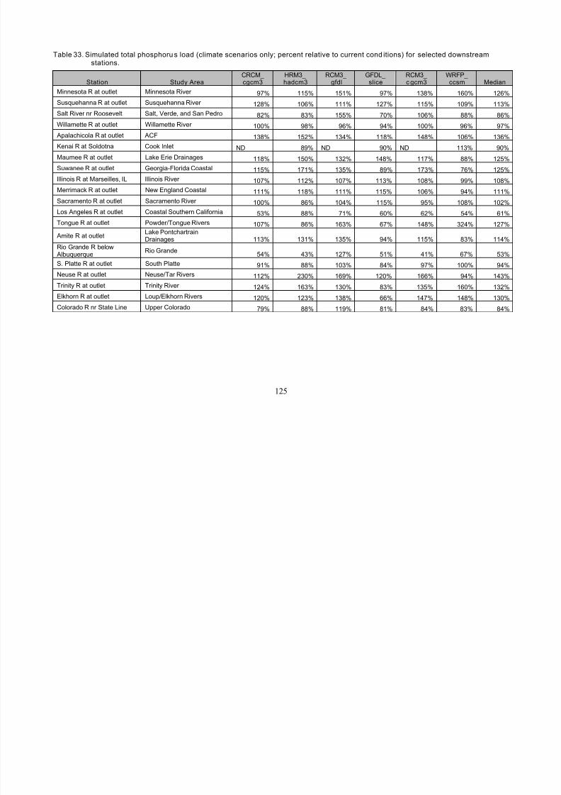
8/13/2019 20 Watersheds Erd
http://slidepdf.com/reader/full/20-watersheds-erd 137/186
Table 33. Simulated total phosphoru s load (climate scenarios only; percent relative to current cond itions) for selected downstream
stations.
Station Study AreaCRCM_ HRM3_ RCM3_ GFDL_ RCM3_ WRFP_
Mediancgcm3 hadcm3 gfdl slice c gcm3 ccsm
Minnesota R at outlet Minnesota River 97% 115% 151% 97% 138% 160% 126%
Susquehanna R at outlet Susquehanna River 128% 106% 111% 127% 115% 109% 113%
Salt River nr Roosevelt Salt, Verde, and San Pedro 82% 83% 155% 70% 106% 88% 86%
Willamette R at outlet Willamette River 100% 98% 96% 94% 100% 96% 97%
Apalachicola R at outlet ACF 138% 152% 134% 118% 148% 106% 136%Kenai R at Soldotna Cook Inlet ND 89% ND 90% ND 113% 90%
Maumee R at outlet Lake Erie Drainages 118% 150% 132% 148% 117% 88% 125%
Suwanee R at outlet Georgia-Florida Coastal 115% 171% 135% 89% 173% 76% 125%
Illinois R at Marseilles, IL Illinois River 107% 112% 107% 113% 108% 99% 108%
Merrimack R at outlet New England Coastal 111% 118% 111% 115% 106% 94% 111%
Sacramento R at outlet Sacramento River 100% 86% 104% 115% 95% 108% 102%
Los Angeles R at outlet Coastal Southern California 53% 88% 71% 60% 62% 54% 61%
Tongue R at outlet Powder/Tongue Rivers 107% 86% 163% 67% 148% 324% 127%
Amite R at outletLake PontchartrainDrainages 113% 131% 135% 94% 115% 83% 114%
Rio Grande R below Albuquerque
Rio Grande54% 43% 127% 51% 41% 67% 53%
S. Platte R at outlet South Platte 91% 88% 103% 84% 97% 100% 94%
Neuse R at outlet Neuse/Tar Rivers 112% 230% 169% 120% 166% 94% 143%Trinity R at outlet Trinity River 124% 163% 130% 83% 135% 160% 132%
Elkhorn R at outlet Loup/Elkhorn Rivers 120% 123% 138% 66% 147% 148% 130%
Colorado R nr State Line Upper Colorado 79% 88% 119% 81% 84% 83% 84%
125
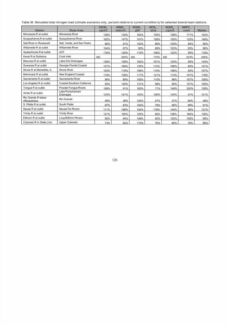
8/13/2019 20 Watersheds Erd
http://slidepdf.com/reader/full/20-watersheds-erd 138/186
Table 34. Simulated total nit rogen load (climate scenarios only; percent relative to current co ndition s) for selected downst ream stations.
Station Study AreaCRCM_ HRM3_ RCM3_ GFDL_ RCM3_ WRFP_
Mediancgcm3 hadcm3 gfdl slice c gcm3 ccsm
Minnesota R at outlet Minnesota River 126% 130% 163% 105% 158% 171% 144%
Susquehanna R at outlet Susquehanna River 162% 147% 147% 156% 150% 132% 149%
Salt River nr Roosevelt Salt, Verde, and San Pedro 90% 91% 142% 86% 105% 84% 90%
Willamette R at outlet Willamette River 104% 97% 95% 89% 103% 93% 96%
Apalachicola R at outlet ACF 116% 125% 115% 106% 122% 95% 116%
Kenai R at Soldotna Cook Inlet ND 200% ND 175% ND 223% 200%
Maumee R at outlet Lake Erie Drainages 128% 158% 162% 191% 125% 94% 143%
Suwanee R at outlet Georgia-Florida Coastal 127% 160% 135% 112% 166% 85% 131%
Illinois R at Marseilles, IL Illinois River 103% 118% 106% 110% 108% 93% 107%
Merrimack R at outlet New England Coastal 119% 128% 117% 121% 114% 101% 118%
Sacramento R at outlet Sacramento River 99% 89% 100% 110% 98% 107% 100%
Los Angeles R at outlet Coastal Southern California 93% 140% 131% 98% 90% 101% 100%
Tongue R at outlet Powder/Tongue Rivers 109% 91% 165% 71% 148% 320% 128%
Amite R at outletLake PontchartrainDrainages 123% 141% 143% 106% 120% 91% 121%
Rio Grande R below Albuquerque
Rio Grande49% 38% 125% 47% 37% 64% 48%
S. Platte R at outlet South Platte 87% 83% 102% 79% 95% 99% 91%
Neuse R at outlet Neuse/Tar Rivers 111% 189% 154% 118% 144% 99% 131%
Trinity R at outlet Trinity River 121% 165% 125% 80% 136% 164% 130%
Elkhorn R at outlet Loup/Elkhorn Rivers 90% 94% 149% 92% 103% 105% 99%
Colorado R nr State Line Upper Colorado 73% 82% 110% 76% 80% 79% 80%
126
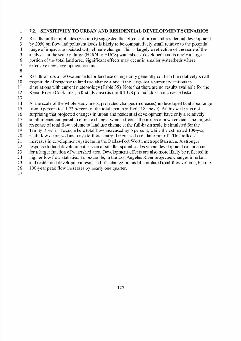
8/13/2019 20 Watersheds Erd
http://slidepdf.com/reader/full/20-watersheds-erd 139/186
1
2
3
45
678
9
1011
12
13
1415
16
1718
19
2021
22
23
2425
26
27
7.2. SENSITIVITY TO URBAN AND RESIDENTIAL DEVELOPMENT SCENARIOS
Results for the pilot sites (Section 6) suggested that effects of urban and residential development
by 2050 on flow and pollutant loads is likely to be comparatively small relative to the potential
range of impacts associated with climate change. This is largely a reflection of the scale of theanalysis: at the scale of large (HUC4 to HUC8) watersheds, developed land is rarely a large
portion of the total land area. Significant effects may occur in smaller watersheds whereextensive new development occurs.
Results across all 20 watersheds for land use change only generally confirm the relatively small
magnitude of response to land use change alone at the large-scale summary stations insimulations with current meteorology (Table 35). Note that there are no results available for the
Kenai River (Cook Inlet, AK study area) as the ICLUS product does not cover Alaska.
At the scale of the whole study areas, projected changes (increases) in developed land area rangefrom 0 percent to 11.72 percent of the total area (see Table 18 above). At this scale it is not
surprising that projected changes in urban and residential development have only a relatively
small impact compared to climate change, which affects all portions of a watershed. The largestresponse of total flow volume to land use change at the full-basin scale is simulated for the
Trinity River in Texas, where total flow increased by 6 percent, while the estimated 100-year
peak flow decreased and days to flow centroid increased (i.e., later runoff). This reflectsincreases in development upstream in the Dallas-Fort Worth metropolitan area. A stronger
response to land development is seen at smaller spatial scales where development can account
for a larger fraction of watershed area. Development effects are also more likely be reflected in
high or low flow statistics. For example, in the Los Angeles River projected changes in urbanand residential development result in little change in model-simulated total flow volume, but the
100-year peak flow increases by nearly one quarter.
127
8/13/2019 20 Watersheds Erd
http://slidepdf.com/reader/full/20-watersheds-erd 140/186
Table 35. Simulated response to projected 2050 changes in urban and residenti al development (percent or days relative to currentconditions) for selected downstream stations.
128
Total 7-day low100-yrpeak
Days toflow
Richards- Baker TSSFlow flow flow centroid flashiness load TP load TN load
Stati on Stud y Area (%) (%) (%) (days ) (%) (%) (%) (%)
Minnesota R at outlet Minnesota River 100.2% 100.3% 99.9% 0.3 100.1% 98.0% 99.3% 99.5%
Susquehanna R at outlet Susquehanna River 100.2% 100.7% 99.7% 0.1 100.1% 100.3% 99.7% 99.2%
Salt River nr Roosevelt Salt, Verde, and San Pedro 100.1% 100.0% 100.2% 0.1 100.3% 100.2% 100.4% 100.2%
Willamette R at outlet Willamette River 99.9% 100.1% 100.1% 0.0 100.7% 99.7% 99.9% 102.5%
Apalachicola R at outlet ACF 100.3% 100.4% 100.3% -0.1 100.0% 100.6% 101.1% 100.5%
Kenai R at Soldotna Cook Inlet ND ND ND ND ND ND ND ND
Maumee R at outlet Lake Erie Drainages 100.5% 100.8% 101.4% 0.2 100.9% 100.6% 101.3% 99.6%
Suwanee R at outlet Georgia-Florida Coastal 100.3% 99.9% 100.6% 0.3 99.5% 100.4% 108.9% 102.5%
Illinois R at Marseilles, IL Illinois River 102.4% 104.0% 102.1% 1.0 98.4% 100.5% 100.2% 99.2%
Merrimack R at outlet New England Coastal 100.4% 100.5% 101.4% 0.0 101.3% 101.2% 103.8% 102.0%
Sacramento R at outlet Sacramento River 100.1% 100.1% 99.9% -0.1 100.4% 99.7% 102.1% 104.7%
Los Angeles R at outletCoastal SouthernCalifornia 103.8% 103.2% 123.2% 0.5 103.1% 109.4% 133.4% 116.3%
Tongue R at outlet Powder/Tongue Rivers 100.0% 100.0% 100.0% 0.0 100.0% 100.0% 100.0% 100.0%
Amite R at outlet
Lake Pontchartrain
Drainages 100.8% 102.6% 101.6% 0.2 100.4% 98.7% 106.8% 103.9%Rio Grande R below Albuquerque
Rio Grande100.1% 100.1% 100.4% 0.0 100.2% 101.1% 95.4% 99.6%
S. Platte R at outlet South Platte 104.0% 101.6% 100.0% 1.1 97.1% 106.0% 102.1% 102.6%
Neuse R at outlet Neuse/Tar Rivers 101.7% 105.2% 102.1% 0.7 99.1% 102.3% 106.7% 103.3%
Trinity R at outlet Trinity River 106.4% 188.1% 74.2% 3.7 68.8% 61.9% 110.0% 106.2%
Elkhorn R at outlet Loup/Elkhorn Rivers 100.3% 100.4% 101.4% 0.0 102.8% 100.1% 100.1% 99.8%
Colorado R nr State Line Upper Colorado 100.1% 100.6% 100.3% -0.1 99.8% 100.0% 100.8% 100.2%
8/13/2019 20 Watersheds Erd
http://slidepdf.com/reader/full/20-watersheds-erd 141/186
1
2
3
45
678
9
1011
12
13
1415
16
1718
19
2021
22
23
2425
26
27
2829
7.3. RELATIVE EFFECTS OF CLIMATE CHANGE AND URBAN DEVELOPMENT
SCENARIOS
The effects of urban and residential development alone were evaluated by comparing the
scenario with current climate and existing land use to the scenario for current climate and futureland use. As shown above (Table 18), ICLUS projected changes in urban and residential
development for 2050 may be important locally but are small relative to the area of large basinsin the study areas. Increased development has long been recognized as a source of hydrologicchanges and water quality degradation at local scales in urbanizing areas (e.g., U.S. EPA, 1984).
The cumulative impacts of development, however, tend to be relatively small at the larger basin
scale evaluated in this study simply because only a small fraction of most HUC4-scalewatersheds is developed or predicted to be developed by 2050.
The relative magnitude of effects from urban development vs. climate change in our simulations
is seen by examining changes in mean annual flow. Figure 37 compares the results of land usechange to the range of climate change effects simulated under the six NARCCAP RCM
downscaled climate projections for the pilot study areas where the HSPF model was applied. The
results summarize the range of responses across selected HUC8 outlets and additional calibrationstations contained within a study area.
Table 36 shows the range of simulated responses of mean annual flow to projected mid-21st
century climate and land use change at the HUC8 and larger scale based on SWAT simulations
for the six NARCCAP climate change scenarios and ICLUS 2050 projected changes in
developed land. Both models show a smaller range of response to projected future changes in
urban development than to projected climate change. At the spatial scale of these simulations projected future changes in impervious cover were relatively small as a percent basis. Thus, the
range of simulated hydrologic response to climate change scenarios was significantly greater
than the response to urban development scenarios. At smaller spatial scales, however, the effects
of urban and residential development could be greater. Results for pollutant loads are similar tothose for streamflow.
129
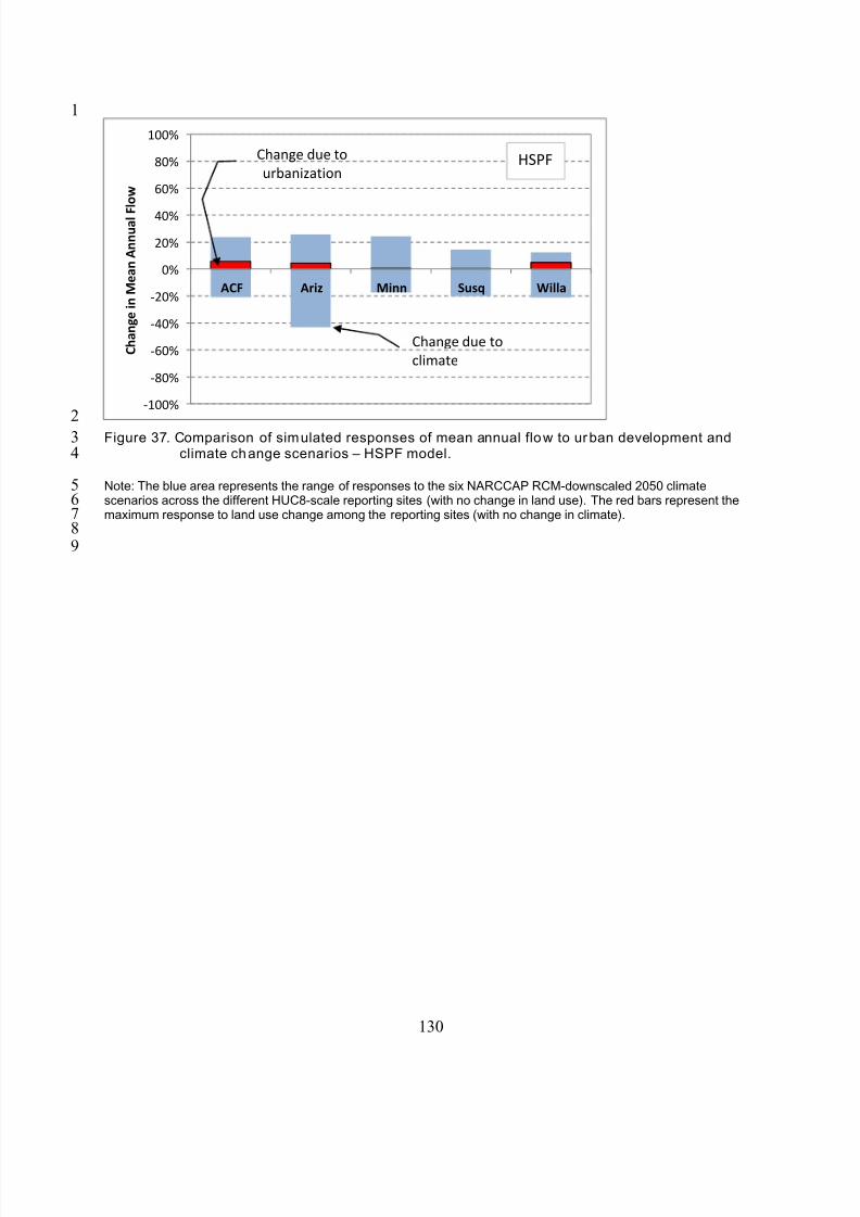
8/13/2019 20 Watersheds Erd
http://slidepdf.com/reader/full/20-watersheds-erd 142/186
1
2
34
56789
130
‐100%
‐80%
‐60%
‐40%
‐20%
0%
20%
40%
60%
80%
100%
ACF Ariz Minn Susq Willa
C h a n g e i n M e a n A n n u a l F
l o w
Change due to
climate
Change due to
urbanizationHSPF
Figure 37. Comparison of simulated responses of mean annual flow to urban development andclimate change scenarios – HSPF model.
Note: The blue area represents the range of responses to the six NARCCAP RCM-downscaled 2050 climatescenarios across the different HUC8-scale reporting sites (with no change in land use). The red bars represent themaximum response to land use change among the reporting sites (with no change in climate).
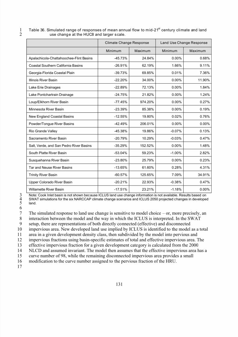
8/13/2019 20 Watersheds Erd
http://slidepdf.com/reader/full/20-watersheds-erd 143/186
12
3456
7
89
10
1112
13
1415
16
17
Table 36. Simulated range of responses of mean annual flow to mid-21st
century climate and landuse change at the HUC8 and larger scale.
Climate Change Response Land Use Change Response
Minimum Maximum Minimum Maximum
Apalachicola-Chattahoochee-Flint Basins -45.73% 24.84% 0.00% 0.68%
Coastal Southern California Basins -26.91% 62.19% 1.66% 9.11%
Georgia-Florida Coastal Plain -39.73% 69.85% 0.01% 7.36%
Illinois River Basin -22.20% 34.00% 0.00% 11.90%
Lake Erie Drainages -22.89% 72.13% 0.00% 1.84%
Lake Pontchartrain Drainage -24.75% 21.82% 0.00% 1.24%
Loup/Elkhorn River Basin -77.45% 974.20% 0.00% 0.27%
Minnesota River Basin -23.39% 85.38% 0.00% 0.19%
New England Coastal Basins -12.55% 19.80% 0.02% 0.76%
Powder/Tongue River Basins -42.49% 206.01% 0.00% 0.00%
Rio Grande Valley -45.38% 19.86% -0.07% 0.13%
Sacramento River Basin -20.79% 10.29% -0.03% 0.47%
Salt, Verde, and San Pedro River Basins -35.29% 152.52% 0.00% 1.48%
South Platte River Basin -53.04% 59.23% -1.00% 2.82%
Susquehanna River Basin -23.80% 25.79% 0.00% 0.23%
Tar and Neuse River Basins -13.65% 61.60% 0.28% 4.31%
Trinity River Basin -60.57% 125.65% 7.09% 34.91%
Upper Colorado River Basin -20.21% 22.93% -0.38% 0.47%
Willamette River Basin -17.51% 23.21% -1.18% 0.00%
Note: Cook Inlet basin is not shown because ICLUS land use change information is not available. Results based onSWAT simulations for the six NARCCAP climate change scenarios and ICLUS 2050 projected changes in developedland.
The simulated response to land use change is sensitive to model choice – or, more precisely, an
interaction between the model and the way in which the ICLUS is interpreted. In the SWATsetup, there are representations of both directly connected (effective) and disconnected
impervious area. New developed land use implied by ICLUS is identified to the model as a total
area in a given development density class, then subdivided by the model into pervious andimpervious fractions using basin-specific estimates of total and effective impervious area. The
effective impervious fraction for a given development category is calculated from the 2000
NLCD and assumed invariant. The model then assumes that the effective impervious area has acurve number of 98, while the remaining disconnected impervious area provides a small
modification to the curve number assigned to the pervious fraction of the HRU.
131
8/13/2019 20 Watersheds Erd
http://slidepdf.com/reader/full/20-watersheds-erd 144/186
1
2
34
5
67
8
9
1011
12
1314
15
16
1718
19
2021
22
2324
25
2627
28
2930
31
32
3334
35
36
3738
394041
42
4344
45
46
In contrast, HSPF has pervious (PERLND) and impervious (IMPLND) land uses, but does not
distinguish a separate disconnected impervious class. For HSPF, the new developed area in
ICLUS is assigned to the relevant pervious and impervious land use fractions based on the basin-specific percent imperviousness for the land use class. In essence, this means that somewhat
greater future connected imperviousness is being specified to the HSPF model than is specified
to the SWAT model. While the two approaches are rather different, they are consistent withtypical modeling practice for the two models.
Several other details of the SWAT modeling process adopted in this study affect results. The
approach to implementing changes in urban development in SWAT was to remove land fromexisting undeveloped and non-exempt land uses and reassign it to new developed classes that
have the parameters of the most dominant soil and lowest HRU slope in the sub-basin. In some
cases (particularly when a sub-basin is already largely developed) the dominant soil in thewatershed may have characteristics different from the soils and slopes of the remaining
undeveloped land. For HSPF, the urban land uses are not associated with a specific soil or HSG.
In addition, a special circumstance occurs in the Willamette SWAT model. In that model, newdeveloped land primarily comes from dense forest cover. The model tends to predict greater
evapotranspiration for urban grass than for intact evergreen forest, which appears to offset
increases in total flow volume due to increased impervious area.
The effects of land use change on simulated flow extremes can be more dramatic in basins where
strong growth is expected, but also tend to be smaller than the range of simulated climateresponses. For example, in the ACF basin, land use change alone can increase the simulated 100
yr flood peak by up to 27 percent, but the range of responses to the six NARCCAP climate
scenarios is from 17 to 66 percent.
7.4. SENSITIVITY TO COMBINED CLIMATE CHANGE AND URBAN
DEVELOPMENT SCENARIOS
Given the relatively small response to projected urban and residential development by 2050,
results of the model scenarios that combine climate change and land use change are generally
consistent with those for the climate scenarios. These results are given for the selected analysisstations in Table 37 through Table 44. Each table is followed by a scatterplot that presents the
same information for the selected downstream station graphically. A map is then presented that
shows change results for each HUC8 pour point in the study area (Figure 38 through Figure 58.
Note the results shown are for the simulations combining climate change with urbandevelopment scenarios, with the exception of the Kenai River in the Cook Inlet basin.
Development projections are not available for Kenai study area, but are anticipated to be small.Results for study sites comprised of a single watershed are shown for a downstream outlet.Results for study sites comprised of multiple adjacent basins are shown for a single
representative basin, typically the largest.
Many study areas also show variability in response among subbasins within the larger watershed.
One figure in each set shows the median values of selected endpoints for the six NARCCAP
scenarios for the individual HUC-8 subbasins within each larger study site. It should be noted,
132
8/13/2019 20 Watersheds Erd
http://slidepdf.com/reader/full/20-watersheds-erd 145/186
1
2
34
5
67
8
9
1011
12
1314
15
16
1718
19
2021
22232425
26
2728
2930
3132
33
3435
36
3738
39
404142
43
4445
46
47
however, that use of the median values alone without taking into account the full range of
simulated responses to all scenarios is potentially misleading. Median values are presented here
only as an indicator of variability within and among study areas and should not alone beconsidered indicative of broad regional trends.
Figure 39 shows annual flow volume responses (median over all six NARCCAP scenarios) foreach modeled HUC8. On this map, a neutral gray tone represents no change from current
conditions (100 percent of current conditions). Reds indicate flow volumes less than current,
with greater intensity reflecting lower flows; greens represent flow volumes greater than current,
with greater intensity reflecting higher flows.Results highlight a number of important regional trends simulated for the 2041-2070 time period
under the A2 emissions scenario. Most notable is the reduction in flow volume in the central
Rockies, accompanied by increases in flow in the northern plains. Only moderate changes areseen for the west coast and Mississippi Valley, while increases generally result for the east coast.
Several things stand out for model-simulated total flow volume changes in Figure 38. The first is
that increases in flow volume for the Kenai River (Cook Inlet basin) are on average larger thanfor other basins. Perhaps more importantly, for a majority of the basins the different downscaled
models do not provide a consistent sign for changes in flow for the 2041-2070 period, with some
simulating increases and some decreases. The models are in complete agreement as to the sign ofchange only for Kenai River (increase). It is also worth noting that the WRFP downscaling of the
CCSM GCM often seems to be an outlier relative to the other models.
Total average annual flow volume tells only part of the story; the timing and intensity of flowsare also important. The detailed results contained in the appendices show seasonal shifts in flow
timing in most of the study areas. At a national scale the number of days (since October 1, start
of the water year) to the flow centroid – the point at which half the flow of an average year isachieved - is a useful summary measure of changes in seasonality. Figure 45 shows that the
centroid of flow comes earlier in the year in model-simulated response to warmer temperaturesfor many of the snow-melt dominated basins, particularly Cook Inlet in Alaska and higher
elevations in the Rockies, but also for many basins in the southeast. The latter result reflectschanges in precipitation timing, with increased winter precipitation and decreased summer
precipitation. Several of the western basins have later dates for the flow centroid due to a
substantial increase in model-simulated spring or summer precipitation relative to wintersnowpack that counteracts the effects of earlier snowmelt.
The geographic distribution of 100-year peak flows (Log-Pearson III) fit is displayed in Figure43 and shows considerably more heterogeneity. Simulated peak flows increase in many basins,
but show less of a clear pattern (Figure 42). Peak flows tend to decline in the area of the
Southwest where total flows decline, while the greatest increases are seen in Alaska and the populated areas of the east and west coast.
Results also suggest a large (factor of 5) increase in low flows for the Kenai River (Figure 40).
This reflects greater dry season melt rates of ice under a warmer climate in Alaska. The modelsalso consistently show severe declines in low flows for the Rio Grande.
133
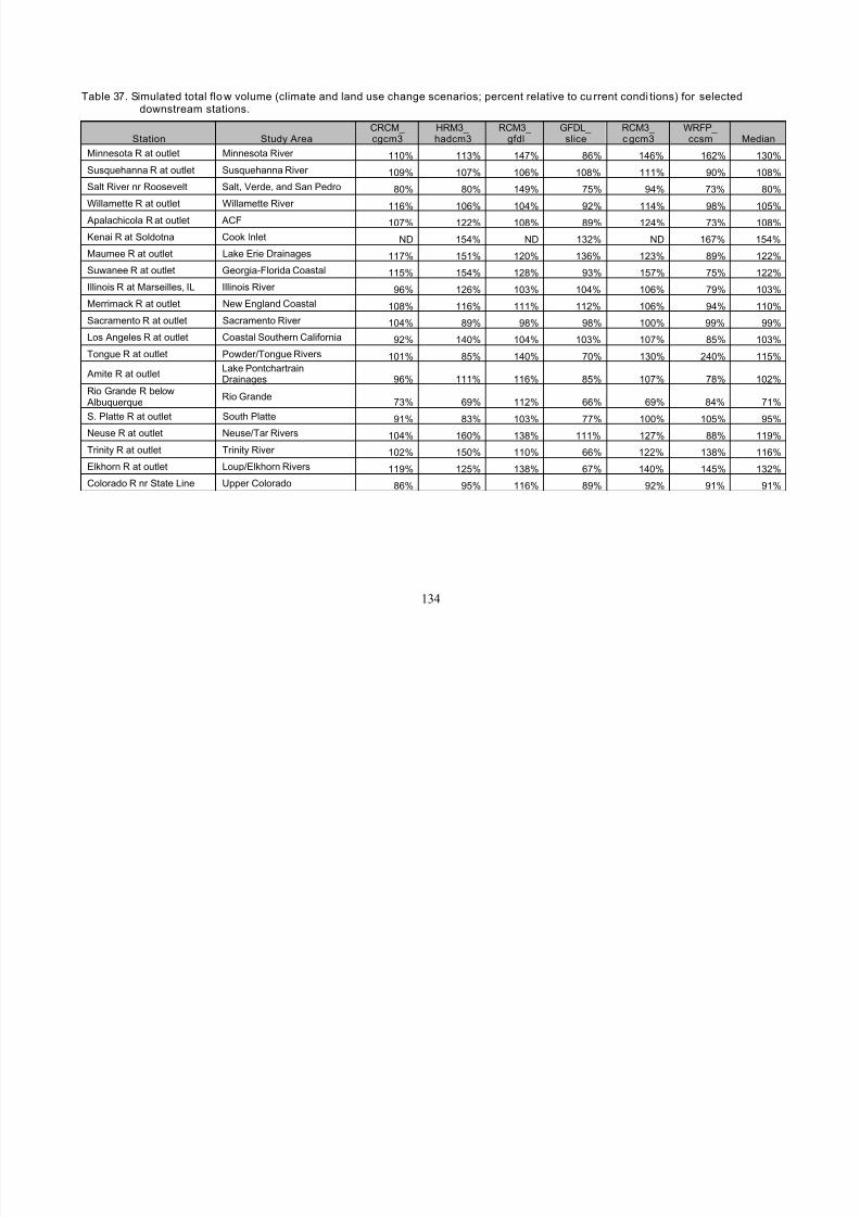
8/13/2019 20 Watersheds Erd
http://slidepdf.com/reader/full/20-watersheds-erd 146/186
Table 37. Simulated total flo w volume (climate and land use change scenarios; percent relative to cu rrent condi tions) for selecteddownstream stations.
Station Study AreaCRCM_ HRM3_ RCM3_ GFDL_ RCM3_ WRFP_
Mediancgcm3 hadcm3 gfdl slice c gcm3 ccsm
Minnesota R at outlet Minnesota River 110% 113% 147% 86% 146% 162% 130%
Susquehanna R at outlet Susquehanna River 109% 107% 106% 108% 111% 90% 108%
Salt River nr Roosevelt Salt, Verde, and San Pedro 80% 80% 149% 75% 94% 73% 80%
Willamette R at outlet Willamette River 116% 106% 104% 92% 114% 98% 105%
Apalachicola R at outlet ACF 107% 122% 108% 89% 124% 73% 108%
Kenai R at Soldotna Cook Inlet ND 154% ND 132% ND 167% 154%
Maumee R at outlet Lake Erie Drainages 117% 151% 120% 136% 123% 89% 122%
Suwanee R at outlet Georgia-Florida Coastal 115% 154% 128% 93% 157% 75% 122%
Illinois R at Marseilles, IL Illinois River 96% 126% 103% 104% 106% 79% 103%
Merrimack R at outlet New England Coastal 108% 116% 111% 112% 106% 94% 110%
Sacramento R at outlet Sacramento River 104% 89% 98% 98% 100% 99% 99%
Los Angeles R at outlet Coastal Southern California 92% 140% 104% 103% 107% 85% 103%
Tongue R at outlet Powder/Tongue Rivers 101% 85% 140% 70% 130% 240% 115%
Amite R at outletLake PontchartrainDrainages 96% 111% 116% 85% 107% 78% 102%
Rio Grande R below Albuquerque
Rio Grande73% 69% 112% 66% 69% 84% 71%
S. Platte R at outlet South Platte 91% 83% 103% 77% 100% 105% 95%
Neuse R at outlet Neuse/Tar Rivers 104% 160% 138% 111% 127% 88% 119%
Trinity R at outlet Trinity River 102% 150% 110% 66% 122% 138% 116%
Elkhorn R at outlet Loup/Elkhorn Rivers 119% 125% 138% 67% 140% 145% 132%
Colorado R nr State Line Upper Colorado 86% 95% 116% 89% 92% 91% 91%
134
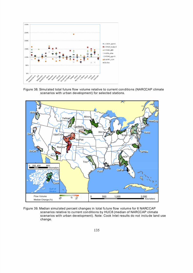
8/13/2019 20 Watersheds Erd
http://slidepdf.com/reader/full/20-watersheds-erd 147/186
Figure 38. Simulated total future flow volume relative to current conditions (NARCCAP climatescenarios with urban development) for selected stations.
135
0 1,000 2,000500Kilometers
Ari z
Sac
Willa
TarNeu
GaFla
Susq
Pont
UppCol
Trin
ACF
NewEng
MinnYellow
Erie
Illin
SoCal
SoPlat
RioGra
CenNeb
Cook
0 400 800200Kilometers
Gulf of
Alaska
Flow Volume
Median Change (%) 2 9
6 - 8 1 0
- 3 7
5 5
Figure 39. Median simulated percent changes in total fu ture flow volume for 6 NARCCAPscenarios relative to cu rrent conditions by HUC8 (median of NARCCAP climatescenarios with urban development). Note: Cook Inlet results do not include land usechange.
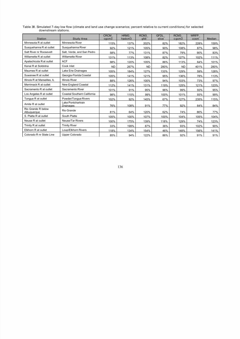
8/13/2019 20 Watersheds Erd
http://slidepdf.com/reader/full/20-watersheds-erd 148/186
Table 38. Simulated 7-day low flow (climate and land use change scenarios; percent relative to cu rrent condi tions) for selecteddownstream stations.
Station Study AreaCRCM_ HRM3_ RCM3_ GFDL_ RCM3_ WRFP_
Mediancgcm3 hadcm3 gfdl slice c gcm3 ccsm
Minnesota R at outlet Minnesota River 115% 137% 202% 82% 182% 228% 159%
Susquehanna R at outlet Susquehanna River 92% 121% 105% 90% 108% 87% 98%
Salt River nr Roosevelt Salt, Verde, and San Pedro 58% 77% 131% 87% 79% 90% 83%
Willamette R at outlet Willamette River 131% 113% 108% 82% 127% 102% 111%
Apalachicola R at outlet ACF 98% 120% 105% 86% 113% 64% 101%
Kenai R at Soldotna Cook Inlet ND 267% ND 280% ND 401% 280%
Maumee R at outlet Lake Erie Drainages 105% 184% 127% 133% 129% 59% 128%
Suwanee R at outlet Georgia-Florida Coastal 105% 141% 121% 95% 136% 78% 113%
Illinois R at Marseilles, IL Illinois River 88% 126% 100% 94% 103% 73% 97%
Merrimack R at outlet New England Coastal 112% 141% 131% 119% 125% 121% 123%
Sacramento R at outlet Sacramento River 101% 91% 95% 96% 99% 93% 95%
Los Angeles R at outlet Coastal Southern California 98% 115% 99% 100% 101% 93% 99%
Tongue R at outlet Powder/Tongue Rivers 102% 92% 145% 67% 127% 235% 115%
Amite R at outletLake PontchartrainDrainages 76% 108% 91% 77% 92% 64% 84%
Rio Grande R below Albuquerque
Rio Grande81% 64% 120% 62% 74% 86% 77%
S. Platte R at outlet South Platte 105% 100% 107% 100% 104% 105% 104%
Neuse R at outlet Neuse/Tar Rivers 100% 175% 139% 118% 129% 74% 123%
Trinity R at outlet Trinity River 33% 199% 87% 36% 93% 102% 90%
Elkhorn R at outlet Loup/Elkhorn Rivers 118% 134% 154% 46% 148% 156% 141%
Colorado R nr State Line Upper Colorado 85% 94% 122% 86% 92% 91% 91%
136
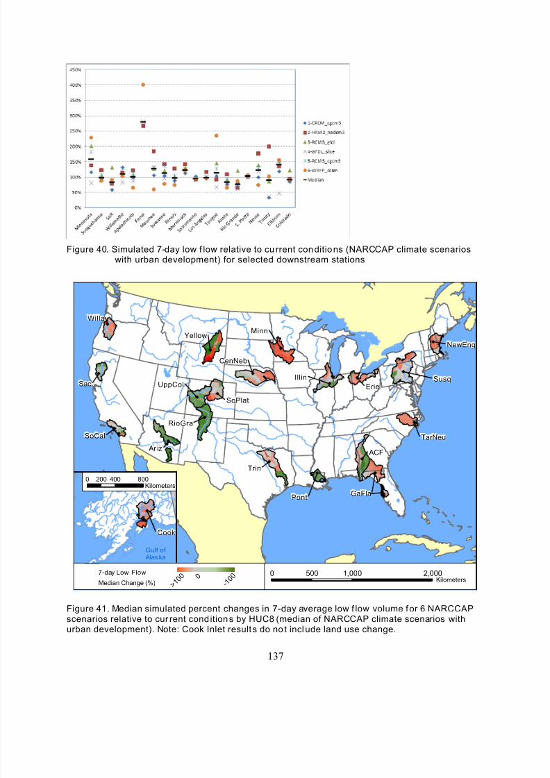
8/13/2019 20 Watersheds Erd
http://slidepdf.com/reader/full/20-watersheds-erd 149/186
Figure 40. Simulated 7-day low f low relative to cu rrent conditions (NARCCAP climate scenarioswith urban development) for selected downstream stations
137
0 1,000 2,000500Kilometers
Ar iz
Sac
Willa
TarNeu
GaFla
Susq
Pont
UppCol
Trin
ACF
NewEng
MinnYellow
Erie
Illin
SoCal
SoPlat
RioGra
CenNeb
Cook
0 400 800200Kilometers
Gulf of
Alas ka
7-day Low Flow
Median Change (%) 2
9 6
- 8 1 0
- 1 0 0
> 1 0 0
Figure 41. Median simulated percent changes in 7-day average low f low volume for 6 NARCCAPscenarios relative to cur rent cond itions by HUC8 (median of NARCCAP climate scenarios withurban development). Note: Cook Inlet results do no t include land use change.
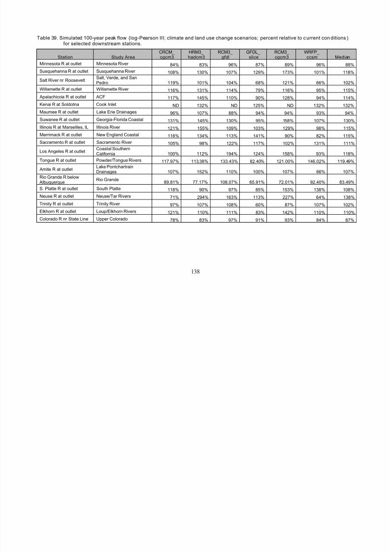
8/13/2019 20 Watersheds Erd
http://slidepdf.com/reader/full/20-watersheds-erd 150/186
Table 39. Simulated 100-year peak flow (log-Pearson III; climate and land use change scenarios; percent relative to c urrent con ditions )
for selected downstream stations.
138
CRCM_ HRM3_ RCM3_ GFDL_ RCM3_ WRFP_Station Study Area cgcm3 hadcm3 gfdl slice cgcm3 ccsm Median
Minnesota R at outlet Minnesota River 84% 83% 96% 87% 89% 96% 88%
Susquehanna R at outlet Susquehanna River 108% 130% 107% 129% 173% 101% 118%
Salt River nr RooseveltSalt, Verde, and SanPedro 119% 101% 104% 68% 121% 66% 102%
Willamette R at outlet Willamette River 116% 131% 114% 79% 116% 95% 115%
Apalachicola R at outlet ACF 117% 145% 110% 90% 128% 94% 114%
Kenai R at Soldotna Cook Inlet ND 132% ND 125% ND 132% 132%
Maumee R at outlet Lake Erie Drainages 96% 107% 88% 94% 94% 93% 94%
Suwanee R at outlet Georgia-Florida Coastal 131% 145% 130% 95% 158% 107% 130%
Illinois R at Marseilles, IL Illinois River 121% 155% 109% 103% 129% 98% 115%
Merrimack R at outlet New England Coastal 116% 134% 113% 141% 90% 82% 115%
Sacramento R at outlet Sacramento River 105% 98% 122% 117% 102% 131% 111%
Los Angeles R at outletCoastal SouthernCalifornia 100% 112% 194% 124% 158% 93% 118%
Tongue R at outlet Powder/Tongue Rivers 117.97% 113.38% 133.43% 82.40% 121.00% 146.02% 119.49%
Amite R at outletLake PontchartrainDrainages 107% 152% 110% 100% 107% 66% 107%
Rio Grande R below Albuquerque
Rio Grande89.81% 77.17% 108.07% 65.91% 72.01% 92.40% 83.49%
S. Platte R at outlet South Platte 118% 90% 97% 85% 153% 138% 108%
Neuse R at outlet Neuse/Tar Rivers 71% 294% 163% 113% 227% 64% 138%
Trinity R at outlet Trinity River 97% 107% 108% 60% 87% 107% 102%
Elkhorn R at outlet Loup/Elkhorn Rivers 121% 110% 111% 83% 142% 110% 110%
Colorado R nr State Line Upper Colorado 78% 83% 97% 91% 93% 84% 87%

8/13/2019 20 Watersheds Erd
http://slidepdf.com/reader/full/20-watersheds-erd 151/186
Figure 42. Simulated 100-yr peak flow relative to current condit ions (NARCCAP climate scenarioswith urban development) for selected downstream stations
139
0 1,000 2,000500Kilometers
Ar iz
Sac
Willa
TarNeu
GaFla
Susq
Pont
UppCol
Trin
ACF
NewEng
MinnYellow
Erie
Illin
SoCal
SoPlat
RioGra
CenNeb
Cook
0 400 800200Kilometers
Gulf of
Alaska
100-year Peak Flow
Median Change (%) 2 9 6
- 8 1 0
- 3 7
> 1 0 0
Figure 43. Median simulated percent changes in 100-year peak flow for 6 NARCCAP scenariosrelative to current condit ions by HUC8 (median of NARCCAP climate scenarios withurban development). Note: Cook Inlet results do not inc lude land use change.
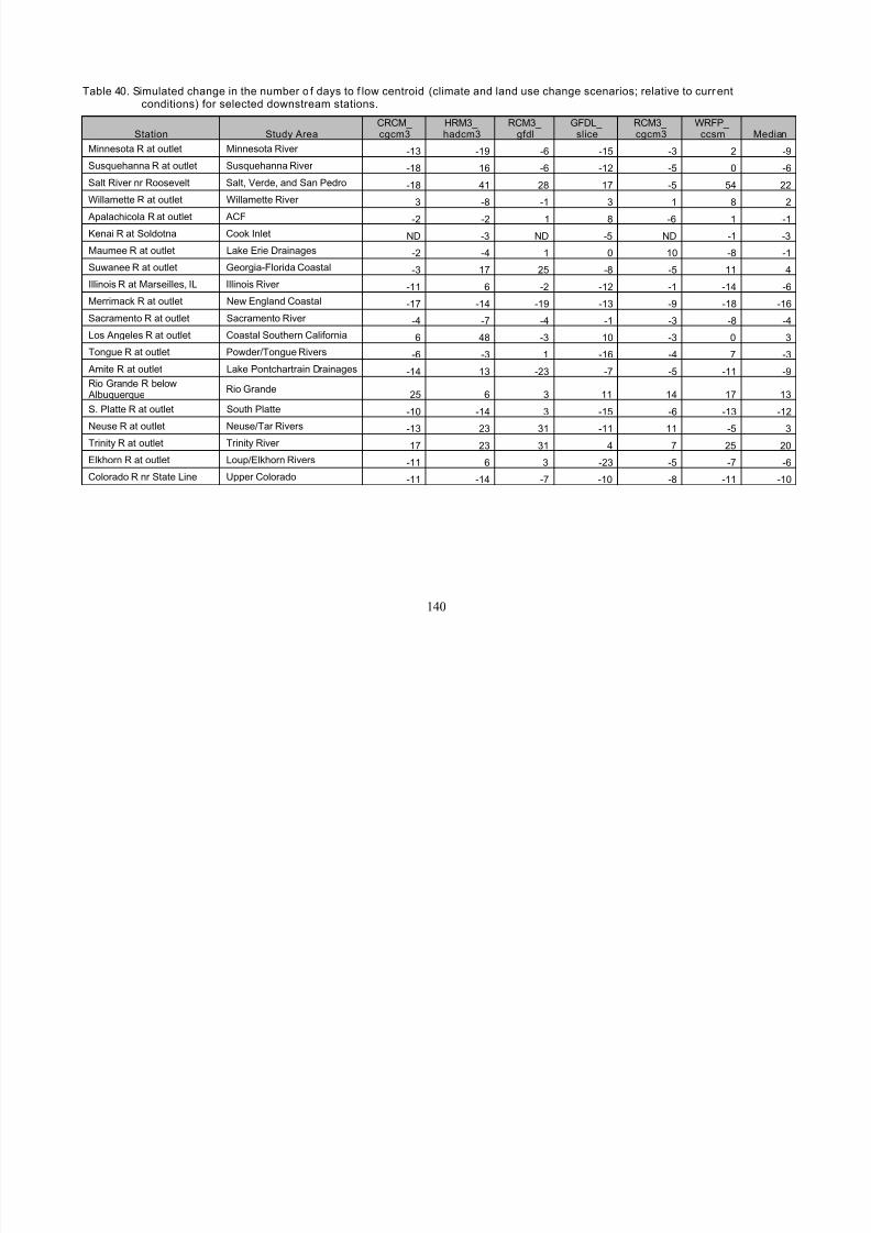
8/13/2019 20 Watersheds Erd
http://slidepdf.com/reader/full/20-watersheds-erd 152/186
Table 40. Simulated change in the number o f days to f low centroid (climate and land use change scenarios; relative to current
conditions) for selected downstream stations.
140
CRCM_ HRM3_ RCM3_ GFDL_ RCM3_ WRFP_Station Study Area cgcm3 hadcm3 gfdl slice cgcm3 ccsm Median
Minnesota R at outlet Minnesota River -13 -19 -6 -15 -3 2 -9
Susquehanna R at outlet Susquehanna River -18 16 -6 -12 -5 0 -6
Salt River nr Roosevelt Salt, Verde, and San Pedro -18 41 28 17 -5 54 22
Willamette R at outlet Willamette River 3 -8 -1 3 1 8 2
Apalachicola R at outlet ACF -2 -2 1 8 -6 1 -1
Kenai R at Soldotna Cook Inlet ND -3 ND -5 ND -1 -3
Maumee R at outlet Lake Erie Drainages -2 -4 1 0 10 -8 -1
Suwanee R at outlet Georgia-Florida Coastal -3 17 25 -8 -5 11 4
Illinois R at Marseilles, IL Illinois River -11 6 -2 -12 -1 -14 -6
Merrimack R at outlet New England Coastal -17 -14 -19 -13 -9 -18 -16
Sacramento R at outlet Sacramento River -4 -7 -4 -1 -3 -8 -4
Los Angeles R at outlet Coastal Southern California 6 48 -3 10 -3 0 3
Tongue R at outlet Powder/Tongue Rivers -6 -3 1 -16 -4 7 -3
Amite R at outlet Lake Pontchartrain Drainages -14 13 -23 -7 -5 -11 -9
Rio Grande R below Albuquerque
Rio Grande25 6 3 11 14 17 13
S. Platte R at outlet South Platte -10 -14 3 -15 -6 -13 -12
Neuse R at outlet Neuse/Tar Rivers -13 23 31 -11 11 -5 3Trinity R at outlet Trinity River 17 23 31 4 7 25 20
Elkhorn R at outlet Loup/Elkhorn Rivers -11 6 3 -23 -5 -7 -6
Colorado R nr State Line Upper Colorado -11 -14 -7 -10 -8 -11 -10
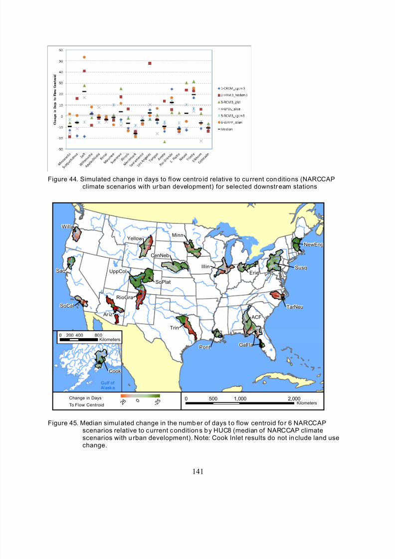
8/13/2019 20 Watersheds Erd
http://slidepdf.com/reader/full/20-watersheds-erd 153/186
Figure 44. Simulated change in days to flow centro id relative to cu rrent conditions (NARCCAPclimate scenarios with urban development) for selected downstream stations
141
0 1,000 2,000500Kilometers
Ar iz
Sac
Willa
TarNeu
GaFla
Susq
Pont
UppCol
Trin
ACF
NewEng
MinnYellow
Erie
Illin
SoCal
SoPlat
RioGra
CenNeb
Cook
0 400 800200Kilometers
Gulf of
Alaska
Change in Days
To Flow Centroid 1 0
- 8 1 0
- 2 5
2 6
Figure 45. Median simulated change in the number of days to flow centroid for 6 NARCCAPscenarios relative to current conditions by HUC8 (median of NARCCAP climatescenarios with urban development). Note: Cook Inlet results do not include land usechange.
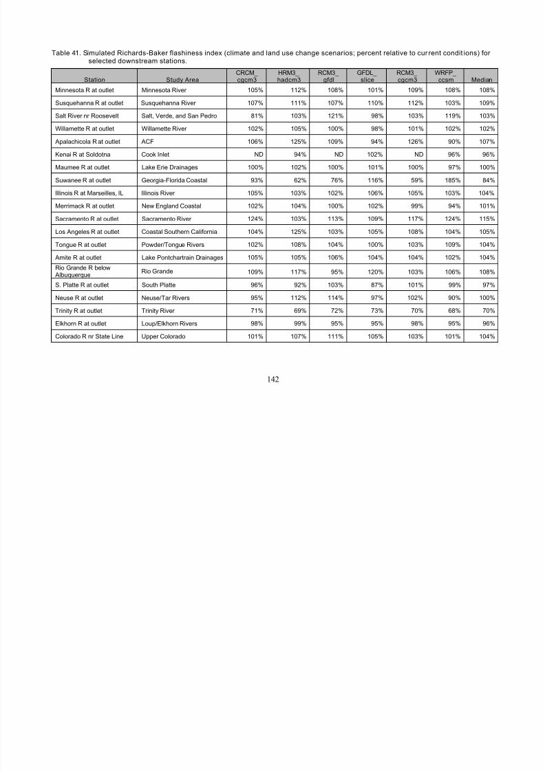
8/13/2019 20 Watersheds Erd
http://slidepdf.com/reader/full/20-watersheds-erd 154/186
Table 41. Simulated Richards-Baker flashiness index (climate and land use change scenarios; percent relative to cur rent condit ions) for
selected downstream stations.
142
CRCM_ HRM3_ RCM3_ GFDL_ RCM3_ WRFP_Station Study Area cgcm3 hadcm3 gfdl slice cgcm3 ccsm Median
Minnesota R at outlet Minnesota River 105% 112% 108% 101% 109% 108% 108%
Susquehanna R at outlet Susquehanna River 107% 111% 107% 110% 112% 103% 109%
Salt River nr Roosevelt Salt, Verde, and San Pedro 81% 103% 121% 98% 103% 119% 103%
Willamette R at outlet Willamette River 102% 105% 100% 98% 101% 102% 102%
Apalachicola R at outlet ACF 106% 125% 109% 94% 126% 90% 107%
Kenai R at Soldotna Cook Inlet ND 94% ND 102% ND 96% 96%
Maumee R at outlet Lake Erie Drainages 100% 102% 100% 101% 100% 97% 100%
Suwanee R at outlet Georgia-Florida Coastal 93% 62% 76% 116% 59% 185% 84%
Illinois R at Marseilles, IL Illinois River 105% 103% 102% 106% 105% 103% 104%
Merrimack R at outlet New England Coastal 102% 104% 100% 102% 99% 94% 101%
Sacramento R at outlet Sacramento River 124% 103% 113% 109% 117% 124% 115%
Los Angeles R at outlet Coastal Southern California 104% 125% 103% 105% 108% 104% 105%
Tongue R at outlet Powder/Tongue Rivers 102% 108% 104% 100% 103% 109% 104%
Amite R at outlet Lake Pontchartrain Drainages 105% 105% 106% 104% 104% 102% 104%
Rio Grande R below Albuquerque
Rio Grande 109% 117% 95% 120% 103% 106% 108%
S. Platte R at outlet South Platte 96% 92% 103% 87% 101% 99% 97%
Neuse R at outlet Neuse/Tar Rivers 95% 112% 114% 97% 102% 90% 100%
Trinity R at outlet Trinity River 71% 69% 72% 73% 70% 68% 70%
Elkhorn R at outlet Loup/Elkhorn Rivers 98% 99% 95% 95% 98% 95% 96%
Colorado R nr State Line Upper Colorado 101% 107% 111% 105% 103% 101% 104%
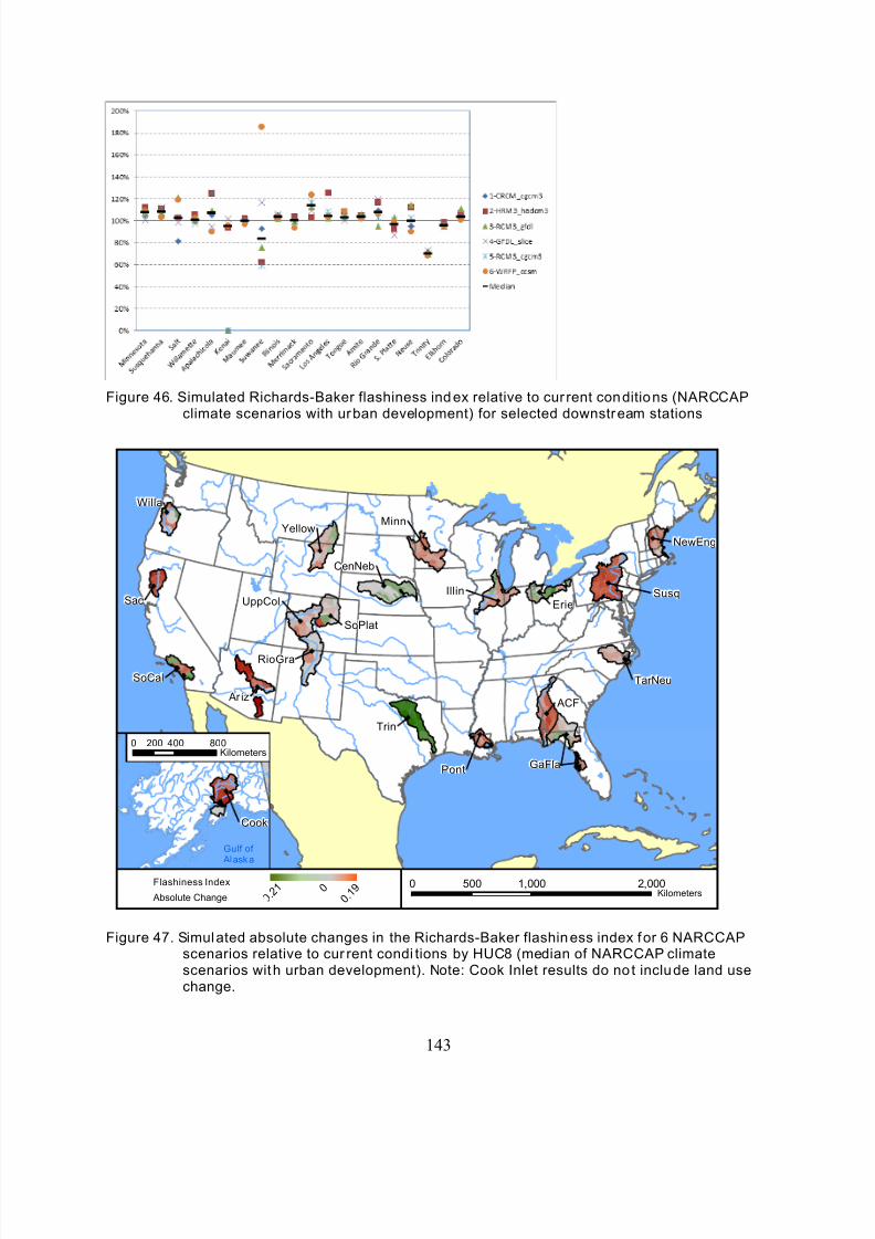
8/13/2019 20 Watersheds Erd
http://slidepdf.com/reader/full/20-watersheds-erd 155/186
Figure 46. Simulated Richards-Baker flashiness index relative to cur rent conditions (NARCCAPclimate scenarios with urban development) for selected downstream stations
143
0 1,000 2,000500Kilometers
Ar iz
Sac
Willa
TarNeu
GaFla
Susq
Pont
UppCol
Trin
ACF
NewEng
MinnYellow
Erie
Illin
SoCal
SoPlat
RioGra
CenNeb
Cook
0 400 800200Kilometers
Gulf of
Alaska
Flashiness Index
Absolute Change 2 9 6
- 8 1 0
0 . 1 9
- 0 . 2 1
Figure 47. Simulated absolute changes in the Richards-Baker flashiness index for 6 NARCCAPscenarios relative to cur rent condi tions by HUC8 (median of NARCCAP climatescenarios with urban development). Note: Cook Inlet results do no t include land usechange.
8/13/2019 20 Watersheds Erd
http://slidepdf.com/reader/full/20-watersheds-erd 156/186
Table 42. Simulated total suspended sol ids load (climate and land use change scenarios; p ercent relative to current co nditions ) for
selected downstream stations.
144
CRCM_ HRM3_ RCM3_ GFDL_ RCM3_ WRFP_Station Study Area cgcm3 hadcm3 gfdl slice cgcm3 ccsm Median
Minnesota R at outlet Minnesota River 104% 117% 183% 76% 192% 219% 150%
Susquehanna R at outlet Susquehanna River 118% 108% 109% 116% 118% 85% 112%
Salt River nr Roosevelt Salt, Verde, and San Pedro 89% 79% 184% 66% 106% 74% 84%
Willamette R at outlet Willamette River 124% 111% 108% 89% 121% 97% 110%
Apalachicola R at outlet ACF 126% 147% 128% 93% 145% 53% 127%Kenai R at Soldotna Cook Inlet ND 234% ND 196% ND 244% 234%
Maumee R at outlet Lake Erie Drainages 123% 170% 127% 154% 130% 87% 128%
Suwanee R at outlet Georgia-Florida Coastal 121% 177% 139% 90% 182% 74% 130%
Illinois R at Marseilles, IL Illinois River 117% 142% 115% 128% 121% 91% 119%
Merrimack R at outlet New England Coastal 119% 129% 119% 123% 112% 86% 119%
Sacramento R at outlet Sacramento River 138% 94% 121% 118% 99% 108% 113%
Los Angeles R at outlet Coastal Southern California 75% 121% 86% 85% 90% 69% 86%
Tongue R at outlet Powder/Tongue Rivers 108% 84% 169% 66% 153% 351% 131%
Amite R at outlet Lake Pontchartrain Drainages 99% 113% 125% 82% 110% 70% 104%
Rio Grande R below Albuquerque
Rio Grande61% 54% 115% 50% 60% 72% 60%
S. Platte R at outlet South Platte 73% 74% 83% 60% 82% 87% 78%
Neuse R at outlet Neuse/Tar Rivers 108% 201% 164% 117% 145% 84% 131%
Trinity R at outlet Trinity River 64% 126% 64% 28% 85% 115% 74%
Elkhorn R at outlet Loup/Elkhorn Rivers 125% 129% 147% 59% 167% 163% 138%
Colorado R nr State Line Upper Colorado 80% 90% 124% 82% 89% 85% 87%
8/13/2019 20 Watersheds Erd
http://slidepdf.com/reader/full/20-watersheds-erd 157/186
Figure 48. Simulated total suspended sol ids load relative to current condit ions (NARCCAP climatescenarios with urban development) for selected downs tream stations.
145
0 1,000 2,000500Kilometers
Ar iz
Sac
Willa
TarNeu
GaFla
Susq
Pont
UppCol
Trin
ACF
NewEng
MinnYellow
Erie
Illin
SoCal
SoPlat
RioGra
CenNeb
Cook
0 400 800200Kilometers
Gulf of
Alaska
Total Suspended Soli ds
Median Change (%) 2 9 6
- 8 1 0
- 9 6
> 1 0 0
Figure 49. Median simu lated percent changes in total suspended solids loads for 6 NARCCAPscenarios relative to cur rent condi tions by HUC8 (median of NARCCAP climatescenarios with urban development) for selected downst ream stations. Note: Cook Inletresults do no t include land use change.
8/13/2019 20 Watersheds Erd
http://slidepdf.com/reader/full/20-watersheds-erd 158/186
Table 43. Simulated total phos phorus l oad (climate and land use change scenarios; percent relative to current conditi ons) for s elected
downstream stations.
Station Study AreaCRCM_ HRM3_ RCM3_ GFDL_ RCM3_ WRFP_
Mediancgcm3 hadcm3 gfdl slice c gcm3 ccsm
Minnesota R at outlet Minnesota River 97% 115% 151% 97% 138% 160% 126%
Susquehanna R at outlet Susquehanna River 128% 106% 110% 127% 114% 108% 112%
Salt River nr Roosevelt Salt, Verde, and San Pedro 82% 84% 156% 70% 107% 88% 86%
Willamette R at outlet Willamette River 100% 98% 97% 94% 100% 96% 97%
Apalachicola R at outlet ACF 139% 153% 136% 119% 150% 107% 138%Kenai R at Soldotna Cook Inlet ND 89% ND 90% ND 113% 90%
Maumee R at outlet Lake Erie Drainages 121% 155% 136% 151% 120% 89% 128%
Suwanee R at outlet Georgia-Florida Coastal 125% 190% 149% 96% 189% 82% 137%
Illinois R at Marseilles, IL Illinois River 107% 112% 107% 113% 108% 99% 107%
Merrimack R at outlet New England Coastal 116% 125% 116% 120% 111% 97% 116%
Sacramento R at outlet Sacramento River 102% 88% 106% 117% 97% 110% 104%
Los Angeles R at outlet Coastal Southern California 78% 128% 102% 83% 89% 71% 86%
Tongue R at outlet Powder/Tongue Rivers 107% 86% 163% 67% 148% 324% 127%
Amite R at outletLake PontchartrainDrainages 123% 144% 147% 103% 125% 89% 124%
Rio Grande R below Albuquerque
Rio Grande51% 40% 125% 49% 37% 64% 50%
S. Platte R at outlet South Platte 93% 90% 106% 85% 99% 102% 96%
Neuse R at outlet Neuse/Tar Rivers 123% 259% 184% 134% 183% 103% 158%Trinity R at outlet Trinity River 148% 188% 153% 98% 155% 187% 154%
Elkhorn R at outlet Loup/Elkhorn Rivers 120% 123% 138% 66% 147% 148% 130%
Colorado R nr State Line Upper Colorado 80% 88% 120% 82% 84% 84% 84%
146

8/13/2019 20 Watersheds Erd
http://slidepdf.com/reader/full/20-watersheds-erd 159/186
Figure 50. Simulated total phosphorus load relative to current condit ions (NARCCAP climatescenarios with urban development) for selected downst ream stations.
147
0 1,000 2,000500Kilometers
Ar iz
Sac
Willa
TarNeu
GaFla
Susq
Pont
UppCol
Trin
ACF
NewEng
MinnYellow
Erie
Illin
SoCal
SoPlat
RioGra
CenNeb
Cook
0 400 800200Kilometers
Gulf of
Alaska
Total Phosphor us
Median Change (%) 2 9 6
- 8 1 0
- 6 7
> 1 0 0
Figure 51. Median simulated percent changes in total phosphorus loads fo r 6 NARCCAP scenariosrelative to current condit ions by HUC8 (median of NARCCAP climate scenarios w ithurban development). Note: Cook Inlet results do not inc lude land use change.
8/13/2019 20 Watersheds Erd
http://slidepdf.com/reader/full/20-watersheds-erd 160/186
Table 44. Simulated total nit rogen load (climate and land use change scenarios; percent relative to cu rrent condit ions) for selected
downstream stations.
Station Study AreaCRCM_ HRM3_ RCM3_ GFDL_ RCM3_ WRFP_
Mediancgcm3 hadcm3 gfdl slice c gcm3 ccsm
Minnesota R at outlet Minnesota River 126% 130% 163% 104% 158% 170% 144%
Susquehanna R at outlet Susquehanna River 161% 146% 146% 155% 149% 131% 147%
Salt River nr Roosevelt Salt, Verde, and San Pedro 90% 91% 142% 87% 105% 85% 91%
Willamette R at outlet Willamette River 106% 98% 97% 91% 105% 95% 97%
Apalachicola R at outlet ACF 117% 126% 116% 107% 123% 96% 117%Kenai R at Soldotna Cook Inlet ND 200% ND 175% ND 223% 200%
Maumee R at outlet Lake Erie Drainages 127% 158% 161% 190% 125% 94% 142%
Suwanee R at outlet Georgia-Florida Coastal 129% 167% 139% 113% 171% 86% 134%
Illinois R at Marseilles, IL Illinois River 103% 117% 105% 109% 107% 93% 106%
Merrimack R at outlet New England Coastal 123% 131% 121% 124% 116% 103% 122%
Sacramento R at outlet Sacramento River 104% 94% 105% 113% 103% 111% 104%
Los Angeles R at outlet Coastal Southern California 125% 159% 154% 102% 96% 101% 113%
Tongue R at outlet Powder/Tongue Rivers 109% 91% 165% 71% 148% 320% 128%
Amite R at outletLake PontchartrainDrainages 130% 152% 153% 113% 127% 95% 128%
Rio Grande R below Albuquerque
Rio Grande50% 38% 127% 48% 37% 65% 49%
S. Platte R at outlet South Platte 89% 86% 106% 80% 97% 101% 93%
Neuse R at outlet Neuse/Tar Rivers 120% 207% 166% 125% 155% 105% 140%Trinity R at outlet Trinity River 140% 187% 142% 93% 153% 186% 148%
Elkhorn R at outlet Loup/Elkhorn Rivers 90% 94% 148% 92% 103% 104% 99%
Colorado R nr State Line Upper Colorado 73% 82% 111% 76% 80% 79% 80%
148
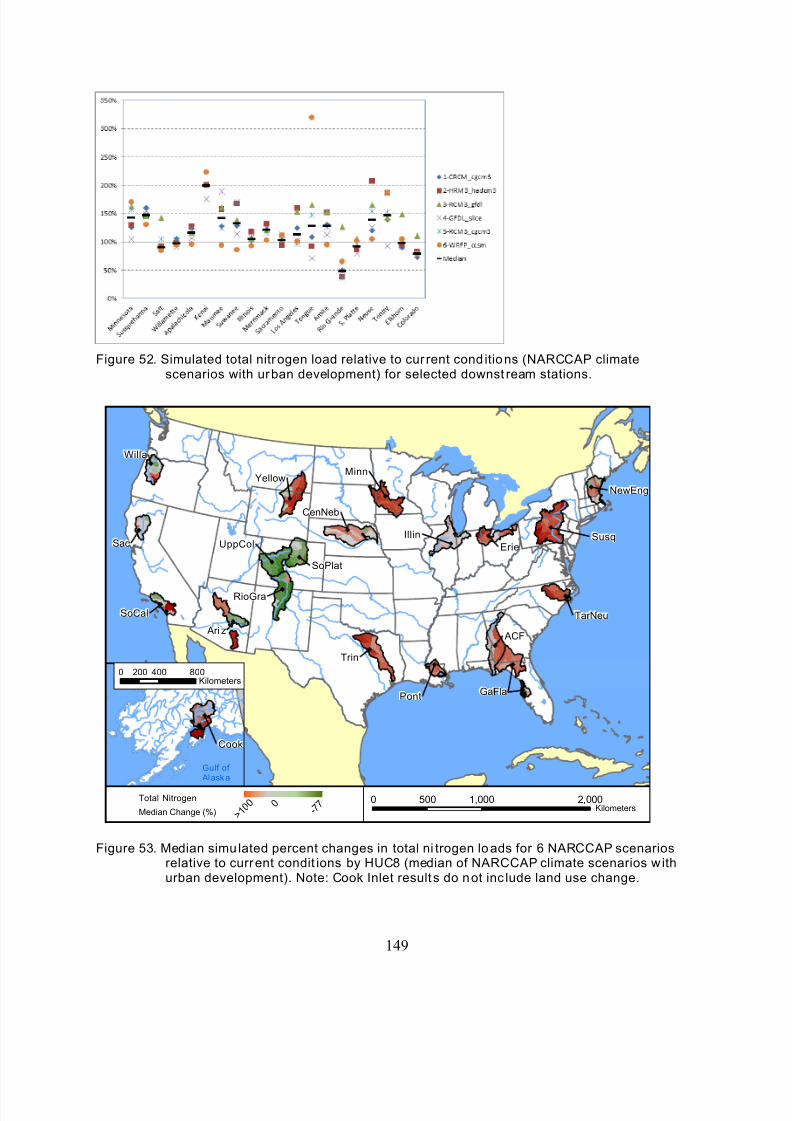
8/13/2019 20 Watersheds Erd
http://slidepdf.com/reader/full/20-watersheds-erd 161/186
Figure 52. Simulated total nitrogen load relative to cur rent cond itions (NARCCAP climate
scenarios with urban development) for selected downst ream stations.
149
0 1,000 2,000500Kilometers
Ari z
Sac
Willa
TarNeu
GaFla
Susq
Pont
UppCol
Trin
ACF
NewEng
MinnYellow
Erie
Illin
SoCal
SoPlat
RioGra
CenNeb
Cook
0 400 800200Kilometers
Gulf of
Alaska
Total Nitrogen
Median Change (%) 2 9 6
- 8 1 0
- 7 7
> 1 0 0
Figure 53. Median simu lated percent changes in total ni trogen loads for 6 NARCCAP scenariosrelative to current condit ions by HUC8 (median of NARCCAP climate scenarios w ithurban development). Note: Cook Inlet results do not inc lude land use change.
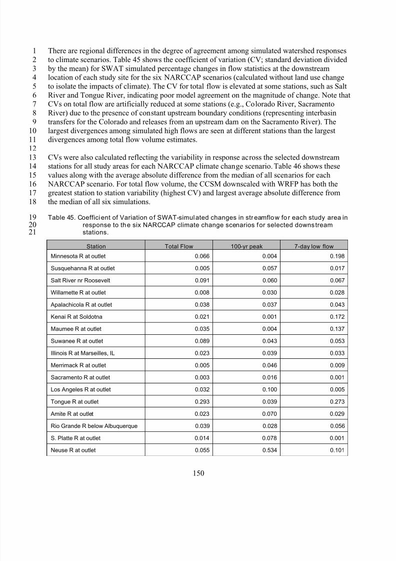
8/13/2019 20 Watersheds Erd
http://slidepdf.com/reader/full/20-watersheds-erd 162/186
1 There are regional differences in the degree of agreement among simulated watershed responses
to climate scenarios. Table 45 shows the coefficient of variation (CV; standard deviation divided
by the mean) for SWAT simulated percentage changes in flow statistics at the downstreamlocation of each study site for the six NARCCAP scenarios (calculated without land use change
to isolate the impacts of climate). The CV for total flow is elevated at some stations, such as Salt
River and Tongue River, indicating poor model agreement on the magnitude of change. Note thatCVs on total flow are artificially reduced at some stations (e.g., Colorado River, Sacramento
River) due to the presence of constant upstream boundary conditions (representing interbasin
transfers for the Colorado and releases from an upstream dam on the Sacramento River). The
largest divergences among simulated high flows are seen at different stations than the largestdivergences among total flow volume estimates.
CVs were also calculated reflecting the variability in response across the selected downstreamstations for all study areas for each NARCCAP climate change scenario. Table 46 shows these
values along with the average absolute difference from the median of all scenarios for each
NARCCAP scenario. For total flow volume, the CCSM downscaled with WRFP has both the
greatest station to station variability (highest CV) and largest average absolute difference fromthe median of all six simulations.
Table 45. Coefficient of Variation o f SWAT-simulated changes in streamflow fo r each study area inresponse to the six NARCCAP climate change scenarios for selected downs treamstations.
2
34
5
67
8
9
01
2
34
5
6
78
901
Station Total Flow 100-yr peak 7-day low flow
Minnesota R at outlet 0.066 0.004 0.198
Susquehanna R at outlet 0.005 0.057 0.017
Salt River nr Roosevelt 0.091 0.060 0.067
Willamette R at outlet 0.008 0.030 0.028
Apalachicola R at outlet 0.038 0.037 0.043
Kenai R at Soldotna 0.021 0.001 0.172
Maumee R at outlet 0.035 0.004 0.137
Suwanee R at outlet 0.089 0.043 0.053
Illinois R at Marseilles, IL 0.023 0.039 0.033
Merrimack R at outlet 0.005 0.046 0.009
Sacramento R at outlet 0.003 0.016 0.001
Los Angeles R at outlet 0.032 0.100 0.005
Tongue R at outlet 0.293 0.039 0.273
Amite R at outlet 0.023 0.070 0.029
Rio Grande R below Albuquerque 0.039 0.028 0.056
S. Platte R at outlet 0.014 0.078 0.001
Neuse R at outlet 0.055 0.534 0.101
11
1
11
1
1
11
122
150
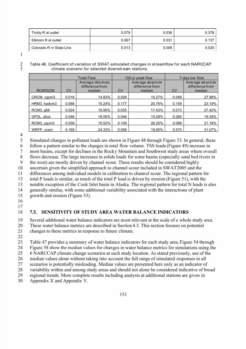
8/13/2019 20 Watersheds Erd
http://slidepdf.com/reader/full/20-watersheds-erd 163/186
Trinity R at outlet 0.079 0.036 0.378
Elkhorn R at outlet 0.067 0.031 0.137
Colorado R nr State Line 0.013 0.006 0.020
1
23
4
56
7
89
10
1112
1314
1516
17
18
1920
21
2223
24
2526
27
28
2930
Table 46. Coefficient of variation of SWAT-simulated changes in st reamflow for each NARCCAPclimate scenario for selected downstream stations .
Total Flow 100-yr peak flow 7day low flow
RCM/GCM CV
Average absolute
CV
Average absolute
CV
Average absolutedifference from difference from difference from
median median median
CRCM_cgcm3 0.016 14.83% 0.028 15.27% 0.058 27.98%
HRM3_hadcm3 0.066 15.24% 0.177 20.76% 0.159 23.19%
RCM3_gfdl 0.024 19.95% 0.035 17.43% 0.073 27.42%
GFDL_slice 0.046 18.05% 0.046 19.28% 0.260 19.39%
RCM3_cgcm3 0.038 15.52% 0.109 26.25% 0.068 21.18%
WRFP_ccsm 0.169 24.33% 0.058 19.65% 0.575 31.07%
Simulated changes in pollutant loads are shown in Figure 48 through Figure 53. In general, thesefollow a pattern similar to the changes in total flow volume. TSS loads (Figure 49) increase in
most basins, except for declines in the Rocky Mountain and Southwest study areas where overall
flows decrease. The large increases in solids loads for some basins (especially sand bed rivers inthe west) are mostly driven by channel scour. These results should be considered highly
uncertain given the simplified approach to channel scour included in SWAT2005 and the
differences among individual models in calibration to channel scour. The regional pattern fortotal P loads is similar, as much of the total P load is driven by erosion (Figure 51), with the
notable exception of the Cook Inlet basin in Alaska. The regional pattern for total N loads is alsogenerally similar, with some additional variability associated with the interactions of plant
growth and erosion (Figure 53).
7.5. SENSITIVITY OF STUDY AREA WATER BALANCE INDICATORS
Several additional water balance indicators are most relevant at the scale of a whole study area.These water balance metrics are described in Section 4.3. This section focuses on potential
changes to these metrics in response to future climate.
Table 47 provides a summary of water balance indicators for each study area. Figure 54 through
Figure 58 show the median values for changes in water balance metrics for simulations using the
6 NARCCAP climate change scenarios at each study location. As stated previously, use of themedian values alone without taking into account the full range of simulated responses to all
scenarios is potentially misleading. Median values are presented here only as an indicator of
variability within and among study areas and should not alone be considered indicative of broad
regional trends. More complete results including analysis at additional stations are given inAppendix X and Appendix Y.
151
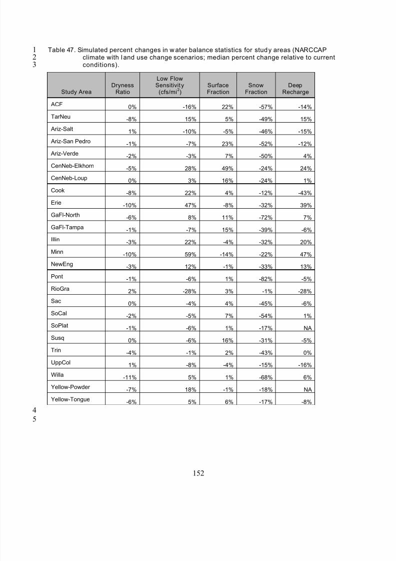
8/13/2019 20 Watersheds Erd
http://slidepdf.com/reader/full/20-watersheds-erd 164/186
1 Table 47. Simulated percent changes in w ater balance statistics for study areas (NARCCAP
climate with l and use change scenarios; median percent change relative to currentconditions).
23
4
5
152
Low FlowDryness Sensitivit y Surface Snow Deep
Study Area Ratio (cfs/mi2) Fraction Fraction Recharge
ACF 0% -16% 22% -57% -14%
TarNeu -8% 15% 5% -49% 15%
Ariz-Salt 1% -10% -5% -46% -15%
Ariz-San Pedro -1% -7% 23% -52% -12%
Ariz-Verde -2% -3% 7% -50% 4%
CenNeb-Elkhorn -5% 28% 49% -24% 24%
CenNeb-Loup 0% 3% 16% -24% 1%
Cook -8% 22% 4% -12% -43%
Erie -10% 47% -8% -32% 39%
GaFl-North -6% 8% 11% -72% 7%
GaFl-Tampa -1% -7% 15% -39% -6%
Illin -3% 22% -4% -32% 20%
Minn -10% 59% -14% -22% 47%
NewEng -3% 12% -1% -33% 13%
Pont -1% -6% 1% -82% -5%
RioGra 2% -28% 3% -1% -28%
Sac 0% -4% 4% -45% -6%
SoCal -2% -5% 7% -54% 1%
SoPlat -1% -6% 1% -17% NA
Susq 0% -6% 16% -31% -5%
Trin -4% -1% 2% -43% 0%
UppCol 1% -8% -4% -15% -16%
Willa -11% 5% 1% -68% 6%
Yellow-Powder -7% 18% -1% -18% NA
Yellow-Tongue -6% 5% 6% -17% -8%

8/13/2019 20 Watersheds Erd
http://slidepdf.com/reader/full/20-watersheds-erd 165/186
1
234
5
678
153
0 1,000 2,000500Kilometers
Ariz
Sac
Willa
TarNeu
GaFla
Susq
Pont
UppCol
Trin
ACF
NewEng
MinnYellow
Erie
Illin
SoCal
SoPlat
RioGra
CenNeb
Cook
0 400 800200Kilometers
Gulf of
Alas ka
Dryness Ratio (ET/P)
Median Change (%) 0
- 1 1
2 . 1
Figure 54. Median simulated percent changes in watershed Dryness Ratio fo r 6 NARCCAPscenarios relative to current condit ions (median of NARCCAP climate scenarios wi thurban development). Note: Cook Inlet results do no t inc lude land use change.
0 1,000 2,000500Kilometers
Ariz
Sac
Willa
TarNeu
GaFla
Susq
Pont
UppCol
Trin
ACF
NewEng
MinnYellow
Erie
Illin
SoCal
SoPlat
RioGra
CenNeb
Cook
0 400 800200Kilometers
Gulf of
Alas ka
Low Flow (cfs / sq mi)
Median Change (%) 0
- 2 8 5 9
Figure 55. Median simulated percent changes in watershed low flow sensiti vity for 6 NARCCAPscenarios relative to current condit ions (median of NARCCAP climate scenarios wi thurban development). Note: Cook Inlet results do not inc lude land use change.
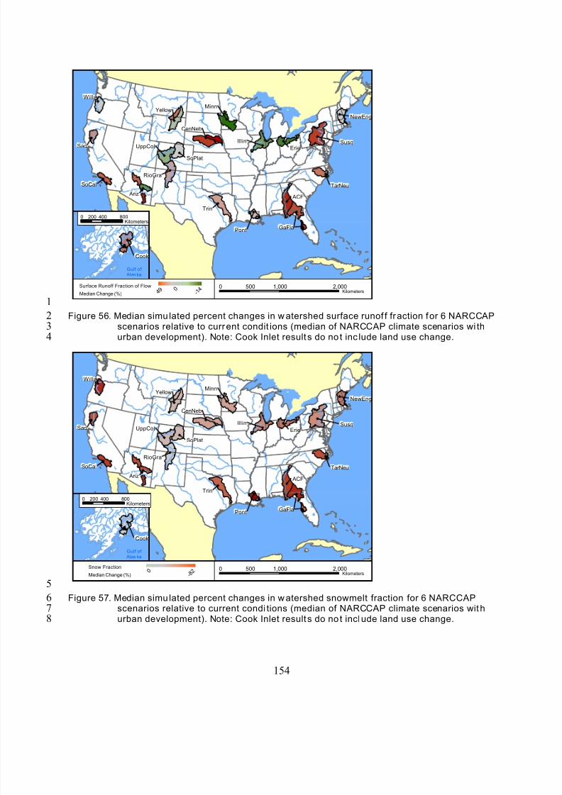
8/13/2019 20 Watersheds Erd
http://slidepdf.com/reader/full/20-watersheds-erd 166/186
1
234
5
678
154
0 1,000 2,000500Kilometers
Ariz
Sac
Willa
TarNeu
GaFla
Susq
Pont
UppCol
Trin
ACF
NewEng
MinnYellow
Erie
Illin
SoCal
SoPlat
RioGra
CenNeb
Cook
0 400 800200Kilometers
Gulf of
Alas ka
Surface Runoff Fraction of Flow
Median Change (%) 0
- 1 4
4 9
Figure 56. Median simu lated percent changes in watershed surface runof f fraction for 6 NARCCAPscenarios relative to current condit ions (median of NARCCAP climate scenarios wi thurban development). Note: Cook Inlet results do no t inc lude land use change.
0 1,000 2,000500Kilometers
Ariz
Sac
Willa
TarNeu
GaFla
Susq
Pont
UppCol
Trin
ACF
NewEng
MinnYellow
Erie
Illin
SoCal
SoPlat
RioGra
CenNeb
Cook
0 400 800200Kilometers
Gulf of
Alas ka
0 - 8 2
Snow Fraction
Median Change (%)
Figure 57. Median simu lated percent changes in watershed snowmelt fraction for 6 NARCCAPscenarios relative to current condi tions (median of NARCCAP climate scenarios withurban development). Note: Cook Inlet results do no t include land use change.
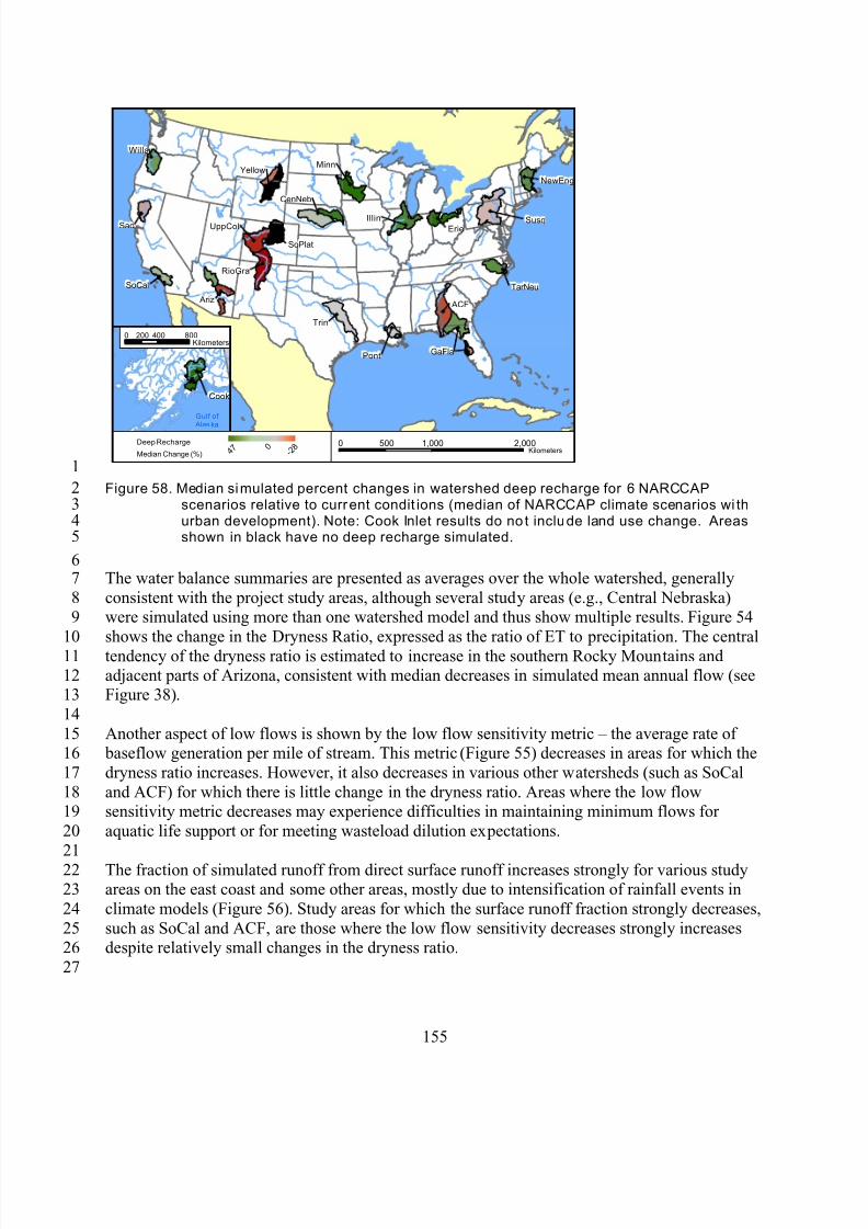
8/13/2019 20 Watersheds Erd
http://slidepdf.com/reader/full/20-watersheds-erd 167/186
1
2345
67
89
10
111213
14
1516
17
1819
20
21
2223
24
2526
27
155
0 1,000 2,000500Kilometers
Ariz
Sac
Willa
TarNeu
GaFla
Susq
Pont
UppCol
Trin
ACF
NewEng
MinnYellow
Erie
Illin
SoCal
SoPlat
RioGra
CenNeb
Cook
0 400 800200Kilometers
Gulf of
Alas ka
Deep Recharge
Median Change (%) 0
- 2 8
4 7
Figure 58. Median simulated percent changes in watershed deep recharge for 6 NARCCAPscenarios relative to current condit ions (median of NARCCAP climate scenarios wi thurban development). Note: Cook Inlet results do no t include land use change. Areasshown in black have no deep recharge simulated.
The water balance summaries are presented as averages over the whole watershed, generally
consistent with the project study areas, although several study areas (e.g., Central Nebraska)were simulated using more than one watershed model and thus show multiple results. Figure 54
shows the change in the Dryness Ratio, expressed as the ratio of ET to precipitation. The central
tendency of the dryness ratio is estimated to increase in the southern Rocky Mountains andadjacent parts of Arizona, consistent with median decreases in simulated mean annual flow (seeFigure 38).
Another aspect of low flows is shown by the low flow sensitivity metric – the average rate of baseflow generation per mile of stream. This metric (Figure 55) decreases in areas for which the
dryness ratio increases. However, it also decreases in various other watersheds (such as SoCal
and ACF) for which there is little change in the dryness ratio. Areas where the low flowsensitivity metric decreases may experience difficulties in maintaining minimum flows for
aquatic life support or for meeting wasteload dilution expectations.
The fraction of simulated runoff from direct surface runoff increases strongly for various studyareas on the east coast and some other areas, mostly due to intensification of rainfall events in
climate models (Figure 56). Study areas for which the surface runoff fraction strongly decreases,
such as SoCal and ACF, are those where the low flow sensitivity decreases strongly increasesdespite relatively small changes in the dryness ratio.

8/13/2019 20 Watersheds Erd
http://slidepdf.com/reader/full/20-watersheds-erd 168/186
1
2
34
5
67
8
9
1011
12
13
14
The fraction of runoff that is due to melting snow (Figure 57) declines in all watersheds. The
strongest declines (in southern and coastal areas) are somewhat misleading, as these watersheds
generally have small amounts of snow. The lesser percentage declines throughout the Rockiesare of greater concern to water management in the west.
The combination of a greater fraction of surface runoff in many watersheds coupled withincreased dryness and reduced total flow in many western watersheds leads to a reduction in
simulated rates of recharge to deep aquifers in many study areas (Figure 58). The risks are
estimated to be particularly acute in the Rockies and the ACF basins. In other areas, increased
precipitation in the models counteracts other forces through mid-century, including the criticalrecharge areas in Central Nebraska.
156
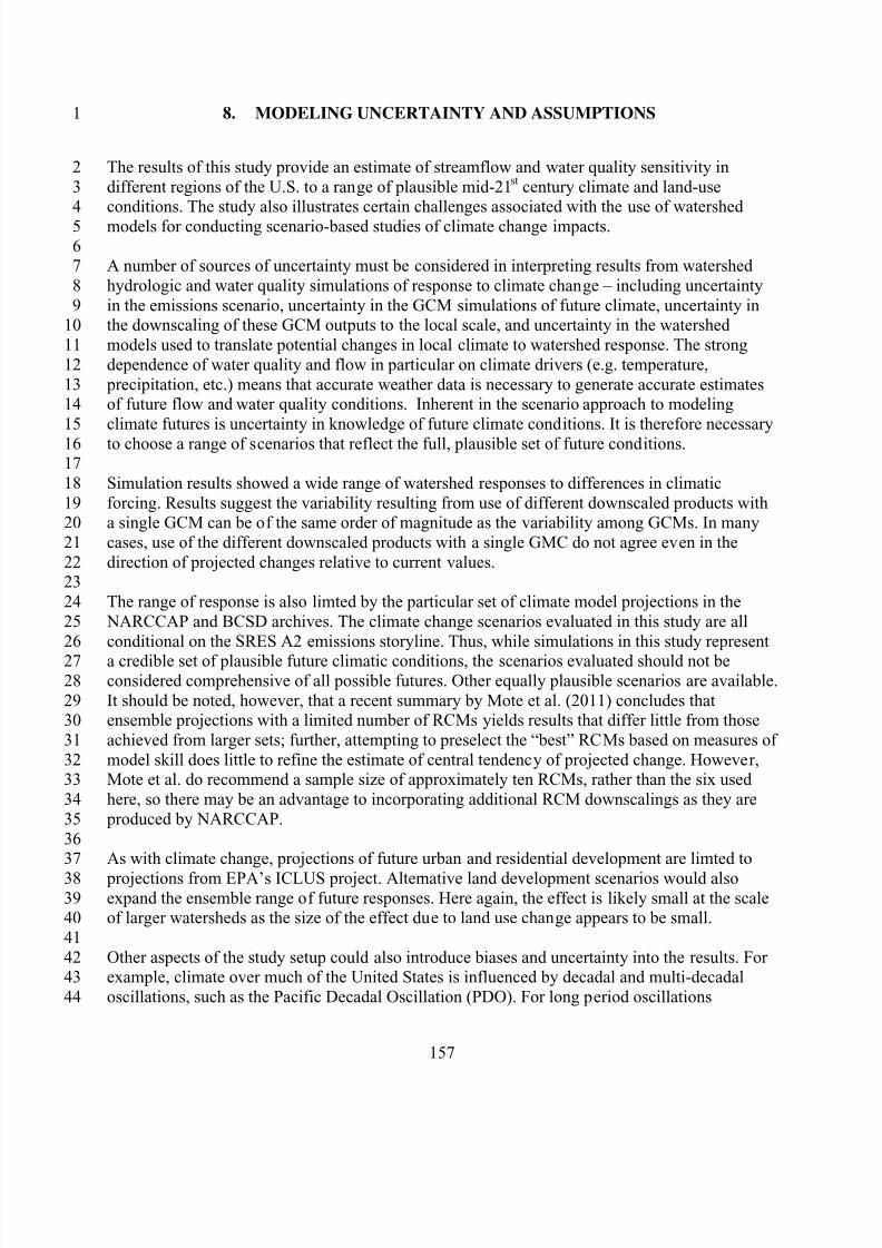
8/13/2019 20 Watersheds Erd
http://slidepdf.com/reader/full/20-watersheds-erd 169/186
5
10
15
20
25
30
35
40
1 8. MODELING UNCERTAINTY AND ASSUMPTIONS
The results of this study provide an estimate of streamflow and water quality sensitivity in
different regions of the U.S. to a range of plausible mid-21st
century climate and land-useconditions. The study also illustrates certain challenges associated with the use of watershed
models for conducting scenario-based studies of climate change impacts.
A number of sources of uncertainty must be considered in interpreting results from watershed
hydrologic and water quality simulations of response to climate change – including uncertainty
in the emissions scenario, uncertainty in the GCM simulations of future climate, uncertainty inthe downscaling of these GCM outputs to the local scale, and uncertainty in the watershed
models used to translate potential changes in local climate to watershed response. The strong
dependence of water quality and flow in particular on climate drivers (e.g. temperature,
precipitation, etc.) means that accurate weather data is necessary to generate accurate estimatesof future flow and water quality conditions. Inherent in the scenario approach to modeling
climate futures is uncertainty in knowledge of future climate conditions. It is therefore necessary
to choose a range of scenarios that reflect the full, plausible set of future conditions.
Simulation results showed a wide range of watershed responses to differences in climatic
forcing. Results suggest the variability resulting from use of different downscaled products witha single GCM can be of the same order of magnitude as the variability among GCMs. In many
cases, use of the different downscaled products with a single GMC do not agree even in the
direction of projected changes relative to current values.
The range of response is also limted by the particular set of climate model projections in the
NARCCAP and BCSD archives. The climate change scenarios evaluated in this study are all
conditional on the SRES A2 emissions storyline. Thus, while simulations in this study represent
a credible set of plausible future climatic conditions, the scenarios evaluated should not beconsidered comprehensive of all possible futures. Other equally plausible scenarios are available.
It should be noted, however, that a recent summary by Mote et al. (2011) concludes thatensemble projections with a limited number of RCMs yields results that differ little from those
achieved from larger sets; further, attempting to preselect the “best” RCMs based on measures of
model skill does little to refine the estimate of central tendency of projected change. However,Mote et al. do recommend a sample size of approximately ten RCMs, rather than the six used
here, so there may be an advantage to incorporating additional RCM downscalings as they are
produced by NARCCAP.
As with climate change, projections of future urban and residential development are limted to
projections from EPA’s ICLUS project. Alternative land development scenarios would alsoexpand the ensemble range of future responses. Here again, the effect is likely small at the scaleof larger watersheds as the size of the effect due to land use change appears to be small.
Other aspects of the study setup could also introduce biases and uncertainty into the results. Forexample, climate over much of the United States is influenced by decadal and multi-decadal
oscillations, such as the Pacific Decadal Oscillation (PDO). For long period oscillations
2
34
67
8
9
11
12
1314
1617
18
19
21
2223
24
26
2728
29
31
3233
34
3637
3839
41
4243
44
157
8/13/2019 20 Watersheds Erd
http://slidepdf.com/reader/full/20-watersheds-erd 170/186
8/13/2019 20 Watersheds Erd
http://slidepdf.com/reader/full/20-watersheds-erd 171/186
1
2
34
5
67
8
9
1011
12
13
14
15
16
1718
19
2021
22
23
2425
26
27
2829
3031
32
3334
35
36
3738
394041
42
43
44
45
46
At a more sophisticated level both natural and human communities are likely to adapt to climate
changes, influencing the watershed response. The SWAT plant growth model takes into accountthe effects of changed climate on plant growth as a function of CO2, temperature, water stress,
and nutrient availability. However, it does not take into account changes in the type of land cover
that may occur as a result of such stresses – either slowly, as through a gradual shifting ofecological niches, or catastrophically, as might occur through drought-induced forest fires.
Human adapations that affect watershed processes will also occur. For example, crop types (or
total area in crops) are likely to change as producers respond to changes in growing season
length and water availability (e.g., Polsky and Easterling, 2001). Simulation models are not yetavailable to provide a credible analysis of such feedback loops at the scale necessary for
evaulating watershed responses.
8.1. MODEL CALIBRATION
Reliably reproducing the baseline period is important for any study of watershed response to
climate change because any biases present in the model calibration are likely to also affect the
future simulations of flow (Prudhomme and Davies, 2009), possibly with non-linearamplification. The experiences of this project emphasize the importance of calibration and
validation for watershed models. With the SWAT model, the ArcSWAT interface gathers model
setup data from readily available spatial coverages and parameter default ranges and will thusrun without calibration. Uncalibrated model results typically provided a poor fit to both the total
and seasonal water balance and pollutant loads and required substantial adjustment. Furthermore,
parameter values established for one HUC8 watershed within a study area were typically not
fully transferable to other portions of the study area, requiring further adjustment.
The calibration process can introduce modeler bias. This could be mitigated through use of an
automated model calibration scheme. We avoided this option based on past experience with the
SWAT and HSPF models in which automated calibration often converges to physicallyunrealistic model parameter sets. It may, however, be advisable to pursue stepwise, guided
model calibration with carefully specified parameter constraints to avoid the effects of user bias,as was done, for example, in recent USGS simulations of watershed-scale flow response to
climate change using the PRMS model (Hay et al., 2011). PRMS, however, addresses flow only
and has a much more parsimonious data set than does SWAT or HSPF. Nonetheless, theadvantages of controlling for modeler bias may make use of a semi-automated calibration
procedure desirable.
The significance of calibration bias is mitigated somewhat by a focus on relative change asopposed to quantitative estimates of future change. If biases are consistent and linear between the
baseline and future condition, the effect of such biases will tend to cancel out when relativechange is calculated. There is, however, no guarantee that biases will be linear. Further testing toevaluate the effects of alternative model calibrations on the simulated response of different study
areas would be desirable.
8.2. WATERSHED MODEL
In selecting watershed models for this project the following model characteristics were
considered important for assessing watershed sensitivity to climate change.
159
8/13/2019 20 Watersheds Erd
http://slidepdf.com/reader/full/20-watersheds-erd 172/186
1
23
4
5
67
8
9
1011
12
13
1415
16
1718
19
2021
22
23
2425
26
27
2829
3031
32
3334
35
36
3738
394041
42
4344
45
• Dynamic simulation with a sub-daily or daily time step to allow evaluation of changes inshort-term variability in hydrologic and water quality response (e.g., high and low flow
events);
• Process-based to allow sensitivity to changes in meteorological inputs;
• Able to incorporate an energy balance approach to potential evapotranspiration;• Able to simulate water quality (as opposed to merely water quantity) responses;
• Widely used and accepted for hydrologic, water quality, and regulatory applications;
• Feasible to apply at the spatial scale of a 20,000 mi2
watershed;
• In the public domain to be transparent and enable ready replication of results;
Based on these considerations, we selected two watershed models for initial application to the
study sites: HSPF and SWAT. Both are public-domain, government-supported models with a
long history of application that meet all the criteria listed above, yet they take somewhat differentapproaches to watershed simulation. Results of simulations in the five pilot study areas showed
that each model performed within commonly accepted standards for watershed models and
generally yielded similar qualities of fit to observed flow and inferred monthly load time series.The eventual decision to conduct simulations with SWAT in the 15 non-pilot study areas was in
largely due to SWAT’s ability to represent influences of CO2 fertilization and other feedback
responses of plant growth to climate change. HSPF does not directly represent this feedback. It isunclear, however, how well SWAT is able to represent the complex processes affecting plant
growth, nutrient dynamics, and water budgets under changing climate. For example, as CO2
levels increase, leaf level reductions in stomatal conductance and evapotranspiration may be
offset by increased plant growth and leaf area. The effects of CO2 on plant growth may also bealtered over time to nutrient limitation (Reich et al., 2006). Further study is required to better
understand how climate change will affect these processes. It should also be noted, however,
that SWAT (as implemented here, using version SWAT2005) is less than ideal for a variety of
reasons, including simplified simulation of direct runoff using a curve number approach, erosion prediction with MUSLE that does not fully incorporate changes in energy that may occur with
altered precipitation regimes; and a simplistic representation of channel erosion processes thatappears unlikely to provide a firm foundation for simulating channel stability responses to
climate change.
These considerations suggest that a more sophisticated watershed model formulation, combining
a plant growth model (as in SWAT) with a more detailed hydrologic simulation would be
preferable for evaluating watershed responses to climate change. However, even if such a model
was available, fully validated, and ready for implementation this would likely require asignificantly higher level of effort for model implementation and calibration.
Comparison of change scenarios using HSPF and SWAT suggests one must proceed withcaution when attempting to estimate even relative aggregate impacts at a national scale through
use of models with different underlying formulations. Specifically, the SWAT model
incorporation of explicit simulation of plant growth and feedback from CO2 fertilization has asignificant impact on results compared to models that do not simulate this effect. A national
synthesis that drew conclusions from a mix of models that did and did not include this effect
160

8/13/2019 20 Watersheds Erd
http://slidepdf.com/reader/full/20-watersheds-erd 173/186
1
2
34
5
67
8
9
1011
12
13
14
could reach erroneous conclusions regarding the relative intensity of impacts in different
geographical areas.
One important, if commonplace, lesson of this effort is that watershed models of the type
employed here require significant site-specific calibration to produce results that reflect observed
conditions – without which, the ability to respond correctly to changes in meteorological andland use forcing is suspect. Water quality calibration is particularly challenging due to limited
amounts of readily available monitoring data. Additional efforts similar to the one presented here
should either focus on watersheds for which well-calibrated models already exist (and the effort
of assembling water quality input and monitoring data from multiple sources has already beencompleted) or allocate sufficient time and budget to conduct detailed, site-specific calibration.
161
8/13/2019 20 Watersheds Erd
http://slidepdf.com/reader/full/20-watersheds-erd 174/186
5
10
15
20
25
30
35
40
1 9. SUMMARY AND CONCLUSIONS
This report describes watershed modeling in 20 large, U.S. drainage basins (15,000-60,000 km2)
to characterize the sensitivity of streamflow, nutrient (N and P) loading, and sediment loading to
a range of potential mid-21st century climate futures, to assess the potential interaction of
climate change and urbanization in these basins, and to improve our understanding ofmethodological challenges associated with integrating existing tools (e.g., climate models,
downscaling approaches, and watershed models) and datasets to address these scientific
questions. Study areas were selected to represent a range of geographic, hydroclimatic,
physiographic, land use, and other watershed attributes. Other important criteria used in siteselection included the availability of necessary data for calibration and validation of watershed
models, and opportunities for leveraging the availability of pre-existing watershed models.
Models were configured by subdividing study areas into modeling units, followed by continuous
simulation of streamflow and water quality for these units using meteorological, land use, soil,
and stream data. A unique feature of this study is the use of a consistent watershed modelingmethodology and a common set of climate and land-use change scenarios in multiple locations
across the nation. Models in each study area are developed for current (1971-2000) observed
conditions, and then used to simulate results under a range of potential mid-21st century (2041-2070) climate change and urban development scenarios. Watershed modeling was conducted at
each study location using the Soil and Water Assessment Tool (SWAT) model and six climate
change scenarios based on dynamically downscaled (50x50 km2) output from four of the GCMs
used in the Intergovernmental Panel on Climate Change (IPCC) 4th Assessment Report for the period 2041-2070 archived by the North American Regional Climate Change Assessment
Program (NARCCAP). Scenarios were created by adjusting historical weather series to represent
projected changes in climate using a change factor approach. To explore the potential interactionof climate change and urbanization, simulations also include urban and residential development
scenarios for each of the 20 study watersheds. Urban and residential development scenarios wereacquired from EPA’s national-scale Integrated Climate and Land Use Scenarios (ICLUS)
project.
In a subset of 5 study areas (the Minnesota River, the Susquehanna River, the Apalachicola-
Chattahoochee-Flint, the Salt/Verde/San Pedro, and the Willamette River Basins), additional
simulations were conducted to assess the variability in simulated watershed response resultingfrom use of different watershed models and different approaches for downscaling GCM climate
change scenarios. In these study areas, watershed simulations were also run with eight additional
scenarios derived from the same four GCMs used in NARCCAP: four scenarios interpolated to
station locations directly from the GCM output, and four scenarios based on bias-corrected and
spatially downscaled (BCSD) climate projections derived from the Coupled ModelIntercomparison Project Phase 3 (CMIP3) described by Maurer et al. (2007). In addition, in these
5 study areas, all scenario simulations were run independently with a second watershedsimulation model, the Hydrologic Simulation Program-FORTRAN (HSPF).
Given the large size of study areas, calibration and validation of all models was completed byfirst focusing on a single HUC8 within the larger study area (preferably one with a good record
23
4
6
7
8
9
11
1213
14
16
17
1819
21
2223
24
26
2728
29
31
32
3334
36
37
3839
41
42
4344
162
8/13/2019 20 Watersheds Erd
http://slidepdf.com/reader/full/20-watersheds-erd 175/186
1
23
4
5
67
8
910
11
1213
14
15
16
1718
1920
21
2223
24
2526
2728
29
30
3132
33
3435
36
3738
39
4041
42
43
4445
46
163
of flow gaging and water quality monitoring data), and then extending the calibration to adjacent
areas with modifications as needed to achieve a reasonable fit at multiple spatial scales.
Large scale global climate model (GCMs) projections are generally consistent in showing a
continued warming trend over the next century (although with sometimes significant regional-
scale disagreements in the magnitude of this warming), but offer a much wider range of plausibleoutcomes in other aspects of local climate – particularly the timing and intensity of precipitation
and the energy inputs (in addition to air temperature) that determine potential evapotranspiration
– that interact to create watershed responses.
The simulated watershed responses to these changes provide an improved understanding of
system sensitivity to potential climate change and urban development scenarios in differentregions of the country, and provide a range of plausible future hydrologic and water quality
change scenarios that can be applied in various planning and scoping frameworks. The results
illustrate a high degree of regional variability in the response of different streamflow and water
quality endpoints to a range of potential mid-21st century climatic conditions in different regions
of the nation. Watershed hydrologic response is determined by the interaction of precipitationand evapotranspiration, while water quality response is largely dependent on hydrology.
Comparison of simulations in all 20 study areas for the 2041-2070 time horizon suggest potentialflow volume decrease in the Rockies and interior southwest, and increases in the east and
southeast coasts. Wetter winters and earlier snowmelt are likely in many of the northern and
higher elevation watersheds. Higher peak flows will also increase erosion and sedimenttransport; loads of nitrogen and phosphorus are also likely to increase in many watersheds.
In many cases, the range of simulated responses across the different climate models anddownscaling methodologies do not agree in direction. The ultimate significance of any given
simulation of future change will depend on local context, including the historical range ofvariability, thresholds and management targets, management options, and interaction with other
stressors. The simulation results in this study do, however, clearly illustrate that the potential
streamflow and water quality response in many areas could be large.
Watershed simulations were run in all study areas with and without projected mid-21st century
changes in urban and residential development. These results suggest that at the HUC8 basin scale
evaluated in this study, watershed sensitivity to projected urban and residential development will be small relative to the changes resulting from climate change. It is important, however, to
qualify this result. At the HUC8 spatial scale, the projected mid-21st century changes in urban
and residential lands represented by scenarios in this study were also small, ranging from <1 to12 percent of total watershed area. The effects of urban development on adjacent water bodies at
higher levels of development are well documented. It is thus likely that at smaller spatial scales
within study areas where the relative fraction of developed land is greater, the effects ofurbanization will be greater. Identifying the scale at which urbanization effects become
comparable to the effects of a changing climate is an important topic for future research.
The simulation results also illustrate a number of methodological issues related to impactsassessment modeling. These include the sensitivities and uncertainties associated with use of
different watershed models, different approaches for downscaling climate change simulations
8/13/2019 20 Watersheds Erd
http://slidepdf.com/reader/full/20-watersheds-erd 176/186
1
23
4
5
67
8
910
11
1213
14
15
16
1718
1920
21
2223
24
2526
2728
29
30
3132
33
3435
36
3738
39
4041
42
43
4445
46
47
164
from global models, and the interaction between climate change and other forcing factors, such
as urbanization and the effects of changes in atmospheric CO2 concentrations onevapotranspiration. Uncertainty associated with differences in emission scenarios and climate
model sensitivities is well known and widely discussed in previous assessments of climate
change impacts on water (e.g., IPCC, 2007; Karl et al., 2009). This study illustrates a potentially
significant additional sensitivity of watershed simulations to the method selected fordownscaling GCM model output. Results of the intercomparison of climate change datasets
suggest that the variability between downscaling of a single GCM with different RCMs can be of
the same order of magnitude as the ensemble variability between GCMs.
This study also suggests potentially important sensitivity of results to the use of different
hydrologic models (HSPF and SWAT in this study), associated with differences in processrepresentation, such as accounting for the influence of increased atmospheric CO2 on
evapotranspiration. One notable insight from these results is that, in many watersheds, climate
change (when precipitation amount and/or intensity is altered), increasing urbanization, and
increasing atmospheric CO2 can have similar or additive effects on streamflow and pollutant
loading, e.g., a more flashy runoff response with higher high flows and lower low flows. Theresults, while useful as guidance for designing and conducting similar impacts assessment
studies, are only a first step in understanding what are likely highly complex and contextdependent relationships. Further study and evaluation of the implications of these and other
questions is necessary for improving the plausibility and relevance of coupled climate-hydrology
simulations, and ultimately for informing resource managers and climate change adaptationstrategies.
It should also be noted that several of the study areas are complex, highly managed systems. Themodels used in this study do not attempt to represent all these operational aspects in full detail.
Moreover, the scenarios considered do not include potential changes in agricultural practices,water demand, other human responses and natural ecosystem changes such as the prevalence of
forest fire or plant disease that will influence streamflow and water quality. Simulations are also
conditional on climate forcing under the A2 emissions storyline, and do not evaluate the
uncertainty in this storyline. Finally, the models used in this study each require calibration, andthe calibration process inevitably introduces potential biases related to the approach taken and
individual modeler choices.
For these reasons, it is important to reiterate that these simulation results are not intended as
forecasts. Rather, the intent of this study is to assess the general sensitivity of underlying
watershed processes to changes in climate and urban development and not to develop detailed, place-based predictions. This information, together with more detailed local knowledge, can be
used to help identify how and where the greatest vulnerabilities are, and ultimately to guide the
development of reasonable and appropriate response strategies to reduce climate risk. Given theinherent uncertainty of the problem, successful climate change adaptation strategies will likely
need to encompass practices and decisions to reduce vulnerabilities across a wide range of
plausible future climatic conditions. Where there are known system thresholds, knowledge of the
range of potential changes can help to identify the need for consideration of future climatechange in water planning. Many of these strategies might also help to reduce the impacts of
other, existing stressors.
8/13/2019 20 Watersheds Erd
http://slidepdf.com/reader/full/20-watersheds-erd 177/186
5
10
15
20
25
30
35
40
45
1 REFERENCES
Alexander, R.B., R.A. Smith, G.E. Schwarz, E.W. Boyer, J.V. Nolan, and J.W. Brakebill. 2008.
Differences in phosphorus and nitrogen delivery to the Gulf of Mexico from the MississippiRiver Basin. Environmental Science and Technology, 42: 822-830.
Allen, R.G., L.S. Pereira, D. Raes, and M. Smith. 1998. Crop Evapotranspiration: Guidelines forComputing Crop Water Requirements. Irrigation and Drainage Paper 56. Food and Agriculture
Organization of the United Nations, Rome.
Allen, R.G., I.A. Walter, R.L. Elliott, T.A. Howell, D. Itenfisu, M.E. Jensen, and R.L. Snyder.
2005. The ASCE Standardized Reference Evapotranspiration Equation. American Society of
Civil Engineers, Reston, VA.
Allan, R.J. 1986. The Role of Particulate Matter in the Fate of Contaminants in Aquatic
Ecosystems. Scientific Series 142. Inland Waters Directorate, Environment Canada, Ottawa.
Apodaca, L.E., N.E. Driver, V.C. Stephens, and N.E. Spahr. 1996. Environmental Setting and
Implications on Water Quality, Upper Colorado River Basin, Colorado and Utah. U.S.
Geological Survey. Water-Resources Investigations Report 95-4263. Denver, Colorado.
Arnold, T.L., D.J. Sullivan, M.A. Harris, F.A. Fitzpatrick, B.C. Scudder, P.M. Ruhl, D.W.
Hanchar, and J.S. Stewart. 1999. Environmental Setting of the Upper Illinois River Basin andImplications for Water Quality. U.S. Geological Survey Water-Resources Investigations Report
98–4268. Urbana, IL.
Baker, D.B., P. Richards, T.T. Loftus, and J.W. Kramer. 2004. A new flashiness index:
Characteristics and applications to Midwestern rivers and streams. Journal of the AmericanWater Resources Association, 40(2): 503-522.
Belitz, K., S.N. Hamlin, C.A. Burton, R. Kent, R.G. Fay, and T. Johnson. 2004. Water Quality in
the Santa Ana Basin, California, 1999–2001. USGS Circular 1238. United States Geological
Survey, Reston, VA.
Berg, E.E., J.D. Henry, C.L. Fastie, A.D. De Volderd, and S.M. Matsuoka. 2006. Spruce beetle
outbreaks on the Kenai Peninsula, Alaska, and Kluane National Park and Reserve, Yukon
Territory: Relationship to summer temperatures and regional differences in disturbance regimes.Forest Ecology and Management , 227: 219-232.
Bernacchi, C.J., B.A. Kimball, D.R. Quarles, S.P. Long, and D.R. Ort. 2007. Decreases instomatal conductance of soybean under open-air elevation of [CO2] are closely coupled with
decreases in ecosystem evapotranspiration. Plant Physiology, 143: 134-144.
Berndt, M.P., H.H. Hatzell, C.A. Crandall, M. Turtora, J.R. Pittman, and E.T. Oaksford. 1998.
Water Quality in the Georgia-Florida Coastal Plain, Georgia and Florida, 1992-96. U. S.
Geological Survey Circular 1151.
2
34
67
8
9
11
12
1314
1617
18
19
21
2223
24
26
2728
29
31
3233
34
3637
3839
41
4243
44
165
8/13/2019 20 Watersheds Erd
http://slidepdf.com/reader/full/20-watersheds-erd 178/186
1
2
34
5
67
8
9
1011
12
1314
15
16
1718
19
2021
22
2324
25
2627
28
2930
31
32
3334
35
3637
38
3940
41
42
4344
Bicknell, B.R., J.C. Imhoff, J.L. Kittle Jr., T.H. Jobes, and A.S. Donigian, Jr. 2001. Hydrological
Simulation Program - Fortran (HSPF). User’s Manual for Release 12. U.S. EPA NationalExposure Research Laboratory, Athens, GA, in cooperation with U.S. Geological Survey, Water
Resources Division, Reston, VA.
Bicknell, B.R., J.C. Imhoff, J.L. Kittle, Jr., T.H. Jobes, and A.S. Donigian, Jr. 2005. HSPF
Version 12.2 User's Manual. National Exposure Research Laboratory, Office of Research and
Development, U.S. Environmental Protection Agency, Athens, GA.
Burwell, R.E., D. R. Timmons and R. F. Holt. 1975. Nutrient transport in surface runoff as
influenced by soil cover and seasonal periods. Soil Science Society of America Journal, 39(3):
523-528.
Caldwell, P.V., G. Sun, S. G. McNulty, E. C. Cohen, and J. A. Moore Myers, 2012. Impacts of
impervious cover, water withdrawals, and climate change on river flows in the conterminous
U.S. Hydrol. Earth Syst. Sci., 16, 2839–2857
Cao, L., G. Bala, K. Caldeira, R. Nemani, and G. Ban-Weiss. 2010. Importance of carbon
dioxide physiological forcing to future climate change. PNAS , 107(21): 9513-9518.
CCSP (Climate Change Science Program). 2008. Weather and Climate Extremes in a Changing
Climate. Regions of Focus: North America, Hawaii, Caribbean, and U.S. Pacific Islands. AReport by the U.S. Climate Change Science Program and the Subcommittee on Global Change
Research. [Thomas R. Karl, Gerald A. Meehl, Christopher D. Miller, Susan J. Hassol, Anne M.
Waple, and William L. Murray (eds.)]. Department of Commerce, NOAA’s National ClimaticData Center, Washington, D.C., USA, 164 pp.
Cordy, G.E., D.J. Gellenbeck, J.B. Gebler, D.W. Anning, A.L. Coes, R.J. Edmonds, J. A.H.Rees, and H.W. Sanger. 2000. Water Quality in the Central Arizona Basins, Arizona, 1995–98.
U.S. Geological Survey Circular 1213. Reston, VA.
Couch, C.A. 1993. Proceedings of the 1993 Georgia Water Resources Conference, held April 20and 21, 1993, at the University of Georgia, Kathryn J. Hatcher, Editor, Institute of Natural
Resources, The University of Georgia, Athens, GA.
Cox, P. and D. Stephenson. 2007. A changing climate for prediction. Science, 317: 207-208.
Crawford, N.H. and R.K. Linsley. 1966. Digital Simulation in Hydrology: Standford WatershedModel IV, Technical Report 39, Department of Civil Engineering, Stanford University, CA.
Dai, A. 2006. Precipitation characteristics in eighteen coupled climate models. Journal of
Climate, 19: 4605-4630.
166
8/13/2019 20 Watersheds Erd
http://slidepdf.com/reader/full/20-watersheds-erd 179/186
1
2
34
5
67
8
9
1011
12
1314
15
16
1718
19
2021
22
2324
25
2627
28
2930
31
32
3334
35
3637
38
3940
41
42
4344
45
46
Dennehy, K.F., D.W. Litke, C.M. Tate, S.L. Qi, P.B. McMahon, B.W. Bruce, R.A. Kimbrough,
and J.S. Heiny. 1998. Water Quality in the South Platte River Basin, Colorado, Nebraska, and
Wyoming, 1992–95. U.S. Geological Survey Circular 1167.
Donigian, A.S. Jr. 2000. HSPF Training Workshop Handbook and CD. Lecture #19: Calibration
and Verification Issues. EPA Headquarters, Washington Information center, 10-14 January,2000. Prepared for U.S. EPA, Office of Water, Office of Science and Technology, Washington,
DC.
Duda, P., J. Kittle, Jr., M. Gray, P. Hummel, and R. Dusenbury. 2001. WinHSPF Version 2.0 AnInteractive Windows Interface to HSPF (WinHSPF) User's Manual. AQUA TERRA
Consultants. Decatur, GA.
Easterling, W.E., N.J. Rosenberg, M.S. McKenney, C.A. Jones, P.T. Dyke, and J.R. Williams.
1992. Preparing the erosion productivity impact calculator (EPIC) model to simulate crop
response to climate change and the direct effects of CO2. Agricultural and Forest Meteorology,
59: 17-34.
Follett, R.F. 1995. Fate and Transport of Nutrients: Nitrogen. Working Paper No. 7. USDA,
Agricultural Research Service, Soil-Plant-Nutrient Research Unit, Fort Collins, Colorado
Garen, D.C. and D.S. Moore. 2005. Curve number hydrology in water quality modeling: Uses,
abuses, and future directions. Journal of the American Water Resources Association, 41(2): 377388.
Garrick, M., C. Cunnane, and J.E. Nash. 1978. A criterion of efficiency for rainfall-runoffmodels. Journal of Hydrology, 36: 375-381.
Gesch, D., M. Oimoen, S. Greenlee, C. Nelson, M. Steuck, and D. Tyler. 2002. The NationalElevation dataset. Photogrammetric Engineering and Remote Sensing, 68(1): 5-11.
Gleckler, P.J., K.E. Taylor, and C. Doutriaux. 2008. Performance metrics for climate models. Journal of Geophysical Research, 113, D06104, doi:10.1029/2007JD008972.
Groisman, P.Y., R.W. Knight, D. Easterling, T.R. Karl, G.C. Hegerle, and V.N. Razuvaev. 2005.
Trends in intense precipitation in the climate record. Journal of Climate, 18:1326–1350.
Gutowski, W. J., Hegerl, G. C., Holland, G. J., Knutson, T. R., Mearns, L. O., Stouffer, R. J.,
Webster, P. J., Wehner, M. F., and Zwiers, F. W. 2008. Causes of observed changes in extremesand projections of future changes, In: T.R. Karl et al., eds., Weather and Climate Extremes in a
Changing Climate. Regions of Focus: North America, Hawaii, Caribbean, and U.S. Pacific
Islands,. U.S. Clim. Change Sci. Prog., Global Change Res., Washington, D. C.
Hawkins, E., and R. Sutton. 2009. The potential to narrow uncertainty in regional climate
predictions. Bulletin of the American Meteorological Society, 90: 1095-1107.
167
8/13/2019 20 Watersheds Erd
http://slidepdf.com/reader/full/20-watersheds-erd 180/186
1
2
34
5
67
8
9
1011
12
1314
15
16
1718
19
2021
22
2324
25
2627
28
2930
31
32
3334
35
3637
38
3940
41
42
4344
45
46
Hay, L.E., S.L. Markstrom, and C. Ward-Garrison. Watershed-scale response to climate change
through the twenty-first century for selected basins across the United States. Earth Interactions,
15: 1-37.
Homer, C., C. Huang, L. Yang, B. Wylie and M. Coan. 2004. Development of a 2001 National
Landcover Database for the United States. Photogrammetric Engineering and Remote Sensing,70(7): 829-840.
Homer, C., J. Dewitz, J. Fry, M. Coan, N. Hossain, C. Larson, N. Herold, A. McKerrow, J.N.
Van Driel, and J. Wickham. 2007. Completion of the 2001 National Land Cover Database for theconterminous United States. Photogrammetric Engineering and Remote Sensing, 73:337-341.
Huntzinger, T.L. and M.J. Ellis. 1993. Central Nebraska River Basins, Nebraska. Water
Resources Bulletin. 29(4): 533-574.
Hurd, B., N. Leary, R. Jones, and J. Smith. 1999. Relative regional vulnerability of water
resources to climate change. Journal of the American Water Resources Association, 35(6): 13991409.
IPCC (Intergovernmental Panel on Climate Change). 2001. Climate Change 2001: The ScientificBasis. Contribution of Working Group I to the Third Assessment Report of the
Intergovernmental Panel on Climate Change [Houghton, J.T.,Y. Ding, D.J. Griggs, M. Noguer,
P.J. van der Linden, X. Dai, K. Maskell, and C.A. Johnson (eds.)]. Cambridge University Press,Cambridge, UK.
IPCC (Intergovernmental Panel on Climate Change). 2007. Climate Change 2007: SynthesisReport - Summary for Policymakers. Available online at: http://www.ipcc.ch/pdf/assessment
report/ar4/syr/ar4_syr_spm.pdf
Jensen, M.E., R.D. Burman, and R.G. Allen. 1990. Evapotranspiration and Irrigation Water
Requirements. ASCE Manuals and Reports on Engineering Practice No. 70. ASCE, New York.
Karl, T.R., Melillo, J.M., and Peterson, T.C. (eds.) (2009). Global Climate Change Impacts in
the United States. Cambridge University Press, 2009.
Kundzewicz, Z. W., L.J. Mata, N.W. Arnell, P. Doll, P. Kabat, B. Jiménez, K.A. Miller, T. Oki,Z. Sen, and I.A. Shiklomanov. 2007. Freshwater resources and their management. In: Climate
Change 2007: Impacts, Adaptation and Vulnerability. Contribution of Working Group II to the
Fourth Assessment Report of the Intergovernmental Panel on Climate Change (ed. by M. L.Parry, O. F. Canziani, J. P. Palutikof, P. J. van der Linden & C. E. Hanson), 173–210. Cambridge
University Press, Cambridge, UK.
Land, L.F., J.B. Moring, P.C. Van Metre, D.C. Reutter, B.J. Mahler, A.A. Shipp, and R.L. Ulery.1998. Water Quality in the Trinity River Basin, Texas, 1992–95 U.S. Geological Survey Circular
1171.
168
8/13/2019 20 Watersheds Erd
http://slidepdf.com/reader/full/20-watersheds-erd 181/186
1
2
34
5
67
8
9
1011
12
1314
15
16
1718
19
2021
22
2324
25
2627
28
2930
31
32
3334
35
3637
38
3940
41
42
4344
45
46
Leakey, A.D.B., E.A. Ainsworth, C.J. Bernacchi, A. Rogers, S.P. Long, and D.R. Ort. 2009.
Elevated CO2 effects on plant carbon, nitrogen, and water relations: six important lessons from
FACE. Journal of Experimental Botany, 60(10): 2859-2876.
Legates, D.R. and G.J. McCabe, Jr. 1999. Evaluating the use of “goodness-of-fit” measures in
hydrologic and hydroclimatic model validation. Water Resources Research, 35(1): 233-241.
Levings, G.W., D.F. Healy, S.F. Richey, and L.F. Carter. 1998. Water Quality in the Rio Grande
Valley, Colorado, New Mexico, and Texas, 1992-95. U.S. Geological Survey Circular 1162.
Lumb, A.M., R.B. McCammon, and J.L. Kittle Jr. 1994. User’s Manual for an Expert System
(HSPEXP) for Calibration of the Hydrological Simulation Program- FORTRAN. USGS Water
Resources Investigation Report 94-4168. U.S. Geological Survey, Reston, VA.
Maurer, E.P., L. Brekke, T. Pruitt, and P.B. Duffy. 2007. Fine-resolution climate projections
enhance regional climate change impact studies. Eos, Transactions of the American Geophysical
Union, 88(47): 504.
McMahon, G. and O. B. Lloyd, Jr. 1995. Water-Quality Assessment of the Albemarle-Pamlico
Drainage Basin, North Carolina and Virginia-- Environmental Setting and Water-Quality Issues.U.S. Geological Survey Open-File Report 95-136. Raleigh, NC.
Mearns, L. 2009. The North American Regional Climate Change Assessment Program(NARCCAP): overview of Phase II results. IOP Conf. Series: Earth and Environmental Science,
6: 022007.
Mesinger, F., G. DiMego, E. Kalnay, K. Mitchell, P.C. Shafran, W. Ebisuzaki, D. Jović, J.
Woollen, E. Rogers, E. Berbery, M.B. Ek, F. Yun, R. Grumbine, W. Higgins, L. Hong, L. Ying,
G. Manikin, D. Parrish, and S. Wei. 2006. North American regional reanalysis. Bulletin of the
American Meteorological Society, 87(3): 343-360.
Monteith, J.L. 1965. Evaporation and the environment. In The State and Movement of Water in
Living Organisms. XIXth Symposium. Society for Exp. Biology, Swansea. CambridgeUniversity Press, pp. 205-234.
Moriasi, D.N., J.G. Arnold, M.W. Van Liew, R.L. Bingner, R.D. Harmel, and T.L. Veith, 2007.Model Evaluation Guidelines for Systematic Quantification of Accuracy in Watershed
Simulations. Transactions of the ASABE , 50(3): 885-900.
Mote, P., L. Brekke, P.B. Duffy, and E. Maurer. 2011. Guidelines for constructing climate
scenarios. Eos, Transactions, American Geophysical Union, 92(31): 257-258.
Myers, D.N., M.A. Thomas, J.W. Frey, S.J. Rheaume, and D.T. Button. 2000. Water Quality inthe Lake Erie-Lake Saint Clair Drainages Michigan, Ohio, Indiana, New York, and
Pennsylvania, 1996–98. U.S. Geological Survey Circular 1203.
169
8/13/2019 20 Watersheds Erd
http://slidepdf.com/reader/full/20-watersheds-erd 182/186
1
2
34
5
67
8
9
1011
12
1314
15
16
1718
19
2021
22
2324
25
2627
28
2930
31
32
3334
35
3637
38
3940
41
42
4344
45
Nash, J.E. and J.V. Sutcliffe. 1970. River flow forecasting through conceptual models, I: A
discussion of principles. Journal of Hydrology, 10: 282-290.
Neitsch, S.L., J.G. Arnold, J.R. Kiniry, and J.R. Williams. 2005. Soil and Water Assessment
Tool, Theoretical Documentation. Grassland, Soil and Water Research Laboratory, USDA
Agricultural Research Service, Temple, TX.
Polsky, C. and W.E. Easterling. 2001. Adaptation to climate variability and change in the US
Great Plains: A multi-scale analysis of Ricardian climate sensitivities. Agriculture Ecosystems &
Environment , 85: 133-144.
Preston, S.D., V.J. Bierman, Jr., and S.E. Silliman. 1989. An evaluation of methods for the
estimation of tributary mass loads. Water Resources Research, 25(6): 1379-1389.
Prudhomme, C. and H. Davies. 2009. Assessing uncertainties in climate change impact analyses
on the river flow regimes in the UK. Par 1: Baseline climate. Climatic Change, 93: 177-195.
Pyke, C., M. Warren, T. Johnson, J. LaGro Jr., J. Scharfenberg, P. Groth, R. Freed, W. Schroeer,
E. Main. 2011. Assessment of low impact development for managing stormwater with changing
precipitation due to climate change. Landscape and Urban Planning, 103(2):166-173.
Raisanen, J. 2007. How reliable are climate models? Tellus, 59A: 2-29.
Reich, P. B., B. A. Hungate, et al. 2006). Carbon-nitrogen interactions in terrestrial ecosystems
in response to rising atmospheric carbon dioxide. Annual Review of Ecology Evolution and
Systematics 37: 611-636.
SCS (Soil Conservation Service). 1972. Hydrology Guide for Use in Watershed Planning.
National Engineering Handbook, Section 4: Hydrology, Supplement A. U.S. Department ofAgriculture, Natural Resources Conservation Service. Washington, D.C.
Southern California Wetlands Recovery Project Information Station website. Undated.
http://www.scwrp.org/index.htm
SRBC (Susquehanna River Basin Commission). 2008. Comprehensive Plan for the Water
Resources of the Susquehanna River Basin. Harrisburg, PA.
Sharpley, A.N. and J.R. Williams, eds. 1990. EPIC – Erosion Productivity Impact Calculator, 1.
Model documentation. U.S. Department of Agriculture, Agricultural Research Service, Tech.Bull. 1768.
Stainforth, D.A., M.R. Allen, E.R. Tredger, and L.A. Smith. 2007. Confidence, uncertainty, and
decision-support relevance in climate predictions. Philosophical Transactions of the Royal
Society, A, 365: 2145-2161.
170
8/13/2019 20 Watersheds Erd
http://slidepdf.com/reader/full/20-watersheds-erd 183/186
1
2
34
5
67
8
9
1011
12
1314
15
16
1718
19
2021
22
2324
25
2627
28
2930
31
32
3334
35
3637
38
3940
41
42
4344
45
46
Stark, J.R., P.E. Hanson, R.M. Goldstein, J.D. Fallon, A.L. Fong, K.E. Lee, S.E. Kroening, and
W.J. Andrews. 2000. Water Quality in the Upper Mississippi River Basin, Minnesota,
Wisconsin, South Dakota, Iowa, and North Dakota, 1995–98. U.S. Geological Survey Circular1211. Reston, VA.
Stockle, C.O., J.R. Williams, N.J. Rosenberg, and C.A. Jones. 1992. A method for estimating thedirect and climatic effects of rising atmospheric carbon dioxide on growth and yield of crops:
Part 1 – Modification of the EPIC model for climate change analysis. Agricultural Systems, 38:
225-238.
Suddick, E.C., and E.A. Davidson. 2012. The Role of Nitrogen in Climate Change and the
Impacts of Nitrogen-Climate Interactions on Terrestrial and Aquatic Ecosystems, Agriculture,and Human Health in the United States: A Technical Report Submitted to the U.S. National
Climate Assessment. North American Nitrogen Center of the International Nitrogen Initiative
(NANC-INI), Woods Hole Research Center, 149 Woods Hole Road, Falmouth, MA, 02540-1644
USA.
Sun, Y., S. Solomon, A. Dai, and R.W. Portmann. 2006. How often does it rain? Journal of
Climate, 19: 916-934.
TAMU (Texas A&M University). 2010. http://swatmodel.tamu.edu/software/arcswat (accessed
1/27/2010)
Tetra Tech. 2008. Quality Assurance Project Plan for Watershed Modeling to Evaluate Potential
Impacts of Climate and Land Use Change on the Hydrology and Water Quality of Major U.S.Drainage Basins. Prepared for Office of Research and Development Global Change Research
Program, U.S. Environmental Protection Agency, Washington, DC.
Tetra Tech. 2008b. Minnesota River Basin Turbidity TMDL and Lake Pepin Excessive Nutrient
TMDL, Model Calibration and Validation Report. Prepared for Minnesota Pollution Control
Agency, St. Paul, MN by Tetra Tech, Inc., Research Triangle Park, NC.
Trenberth, K.E., P.D. Jones, P. Ambenje, R. Bojariu, D. Easterling, A. Klein Tank, D. Parker, F.
Rahimzadeh, J.A. Renwick, M. Rusticucci, B. Soden, and P. Zhai. 2007. Observations: Surface
and atmospheric climate change. In Climate Change 2007: The Physical Science Basis,
Contribution of Working Group I to the Fourth Assessment Report of the Intergovernmental
Panel on Climate Change, S. Solomon, D. Qin, M. Manning, Z. Chen, M. Marquis, K.B. Averyt,
M. Tignor, and H.L. Miller (eds.). Cambridge University Press, Cambridge, UK and New York.
Ulery, R.L., P.C. Van Metre, and A.S. Crossfield. 1993. Trinity River Basin, Texas: Water
Resources Bulletin, 29(4): 685-711.
USDA (United States Department of Agriculture). 1991. State Soil Geographic (STATSG0)
Data Base; Data Use Information. Miscellaneous Publication 1492. National Soil Survey Center,
Natural Resources Conservation Service, U.S. Dept. of Agriculture, Fort Worth, TX.
171
8/13/2019 20 Watersheds Erd
http://slidepdf.com/reader/full/20-watersheds-erd 184/186
1
2
34
5
67
8
9
1011
12
1314
15
16
1718
19
2021
22
2324
25
2627
28
2930
31
32
3334
35
3637
38
3940
41
42
4344
45
46
U.S. EPA (United States Environmental Protection Agency). 1984. Report to Congress:
Nonpoint Source Pollution in the U.S. Water Planning Division, U.S. Environmental ProtectionAgency, Washington, DC.
U.S. EPA (United States Environmental Protection Agency). 2000. Estimating Hydrology andHydraulic Parameters for HSPF. BASINS Technical Note 6. EPA-823-R00-012. Office of
Water, U.S. Environmental Protection Agency, Washington, DC.
U.S. EPA (United States Environmental Protection Agency). 2001. BASINS Version 3.0 User’sManual. EPA-823-B-01-001. Office of Water, U.S. Environmental Protection Agency,
Washington, DC.
U.S. EPA (United States Environmental Protection Agency). 2002. Nitrogen: Multiple and
Regional Impacts. EPA-430-R-01-006. U.S. Environmental Protection Agency Clean Air
Markets Division, Washington, DC.
U.S. EPA (United States Environmental Protection Agency). 2008. Using the BASINS
Meteorological Database (Version 2006). BASINS Technical Note 10. Office of Water, U.S.
Environmental Protection Agency, Washington, DC.
U.S. EPA (United States Environmental Protection Agency). 2009a. Global Change. National
Center for Environmental Research. U.S. Environmental Protection Agency.www.epa.gov/ncer/science/globalclimate/ (accessed 1/12/2010).
U.S. EPA (United States Environmental Protection Agency). 2009b. BASINS 4.0 – Fact Sheet.http://www.epa.gov/waterscience/BASINS/fs-basins4.html (accessed January 27, 2010).
U.S. EPA (United States Environmental Protection Agency). 2009c. BASINS 4.0 ClimateAssessment Tool (CAT): Supporting Documentation and User’s Manual. EPA/600/R-8/088F.
Global Change Research Program, National Center for Environmental Assessment, Office of
Research and Development, U.S. Environmental Protection Agency, Washington, DC.
U.S. EPA (United States Environmental Protection Agency). 2009d. ICLUS V1.2 User’s
Manual: ArcGIS Tools and Datasets for Modeling US Housing Density Growth. EPA/600/R
09/143A. Global Change Research Program, National Center for Environmental Assessment,Office of Research and Development, U.S. Environmental Protection Agency, Washington, D.C.
U.S. EPA (United States Environmental Protection Agency). 2010. NHDPlus User Guide. Officeof Water, U.S. Environmental Protection Agency, Washington, DC. http://www.horizon
systems.com/nhdplus/documentation.php (accessed 1/12/2010).
USGS (United States Geological Survey). 1982. Guidelines for Determining Flood FlowFrequency. Bulletin #17B of the Hydrology Subcommittee, Interagency Advisory Committee on
Water Data. U.S. Geological Survey, Reston, VA.
172
8/13/2019 20 Watersheds Erd
http://slidepdf.com/reader/full/20-watersheds-erd 185/186
1
2
34
5
67
8
9
1011
12
1314
15
16
1718
19
2021
22
2324
25
2627
28
2930
31
32
3334
35
3637
38
3940
41
42
4344
45
46
USGS (United States Geological Survey). 2001. National Water Quality Assessment (NAWQA)
Program: Willamette Basin Study Unit. http://or.water.usgs.gov/projs_dir/pn366/nawqa.html
Accessed June 2009.
USGS (United States Geological Survey). 2002. National Water Quality Assessment (NAWQA)
Program: The Acadian-Pontchartrain Study Unit . http://la.water.usgs.gov/nawqa/ Accessed June2009.
USGS (United States Geological Survey). 2004. National Water Quality Assessment (NAWQA)
Program: Central Arizona Basins. http://az.water.usgs.gov/cazb/ Accessed June 2009.
USGS (United States Geological Survey). 2006. National Water Quality Assessment (NAWQA)
Program: Upper Colorado River Basin Study Unit. http://co.water.usgs.gov/nawqa/ucol/Accessed June 2009.
USGS (United States Geological Survey). 2007a. National Water Quality Assessment
(NAWQA) Program: Georgia-Florida Coastal Plain Drainages Study Unit.http://fisc.er.usgs.gov/NAWQA/ Accessed June 2009.
USGS (United States Geological Survey). 2007b. National Water-Quality Assessment(NAWQA) Program: New England Coastal Basins (NECB) Study Unit.
http://nh.water.usgs.gov/projects/nawqa/nawqaweb.htm. Accessed June 2009.
USGS (United States Geological Survey). 2007c. National Water Quality Assessment
(NAWQA) Program: Sacramento River Basin. http://ca.water.usgs.gov/sac_nawqa/ Accessed
June 2009.
USGS (United States Geological Survey). 2008a. National Water Quality Assessment
(NAWQA) Program: Apalachicola-Chattahoochee-Flint (ACF) Basin Study.http://ga.water.usgs.gov/nawqa/ Accessed June 2009.
USGS (United States Geological Survey). 2008b. National Water Quality Assessment
(NAWQA) Program: Cook Inlet Basin Study Unit. http://ak.water.usgs.gov/Projects/Nawqa/Accessed June 2009.
USGS (United States Geological Survey). 2008c. National Water Quality Assessment(NAWQA) Program: South Platte River Basin. http://co.water.usgs.gov/nawqa/splt/ Accessed
June 2009.
USGS (United States Geological Survey). 2009a. National Water-Quality Assessment
(NAWQA) Program: Rio Grande Valley. http://nm.water.usgs.gov/nawqa/riog/ Accessed June
2009.
USGS (United States Geological Survey). Undated. National Water-Quality Assessment
Program: New England Coastal Basins. U.S. Geological Survey Fact Sheet FS-060-97.
http://pubs.water.usgs.gov/fs06097 Accessed June 17, 2009.
173
8/13/2019 20 Watersheds Erd
http://slidepdf.com/reader/full/20-watersheds-erd 186/186
1
2
34
5
67
8
9
1011
12
1314
15
16
1718
19
Wang, S.-Y., R.R. Gillies, E.S. Takle, and W.J. Gutowski, Jr. 2009. Evaluation of precipitation
in the Intermountain Region as simulated by the NARCCAP regional climate models.Geophysical Research Letters, 36, L11704, doi:10:1029/2009GL037930.
Warner, K. 1998. Water-Quality Assessment of the Lower Illinois River Basin: EnvironmentalSetting. U.S. Geological Survey. Water-Resources Investigations Report 97–4165. Urbana, IL.
Westerling, A.L., H.G. Hidalgo, D.R. Cayan, and T.W. Swetnam. 2006. Warming and earlier
spring increases western U.S. forest wildfire activity. Science, 313: 940-943.
Wilcox, B.P., W.J. Rawls, D.L. Brakensiek, and J.R. Wight. 1990. Predicting runoff from
rangeland catchments: A comparison of two models. Water Resources Research, 26: 2401-2410.
Williams, J.R. 1975. Sediment-yield prediction with universal equation using runoff energy
factor. pp. 244-252 in Present and Prospective Technology for Predicting Sediment Yield and
Sources: Proceedings of the Sediment-Yield Workshop, USDA Sedimentation Lab, Oxford, MS, November 28-30, 1972. ARSS-40.