Statistical Data Analysis

Lecture 1 MDAS presentationLecture 2 Probability, Bayes’ theorem, Random variables and probability densitiesLecture 3 Catalogue of pdfs (uni-dimensional)Lecture 4 Catalogue of pdfs (multi-dimensional)

Histograms & Probability Density Function

Random variables and probability density functions

A random variable is a numerical characteristic assigned to an element of the sample space; can be discrete or continuous.

Suppose outcome of experiment is continuous value x

→ f(x) = probability density function (pdf)

Or for discrete outcome xi with e.g. i = 1, 2, ... we have

x must be somewhere

probability mass function

x must take on one of its possible values

Cumulative distribution function

Probability to have outcome less than or equal to x is

cumulative distribution function

Alternatively define pdf with

Expectation valuesConsider continuous r.v. x with pdf f (x).

Define expectation (mean) value as

Notation (often): ~ “centre of gravity” of pdf.

For a function y(x) with pdf g(y), (equivalent)

Variance:

Notation:

Standard deviation:

~ width of pdf, same units as x.

Binomial distributionConsider N independent experiments (Bernoulli trials):

outcome of each is ‘success’ or ‘failure’,

probability of success on any given trial is p.

Define discrete r.v. n = number of successes (0 ≤ n ≤ N).

Probability of a specific outcome (in order), e.g. ‘ssfsf’ is

But order not important; there are

ways (permutations) to get n successes in N trials, total

probability for n is sum of probabilities for each permutation.

Binomial distribution (2)The binomial distribution is therefore

randomvariable

parameters

For the expectation value and variance we find:

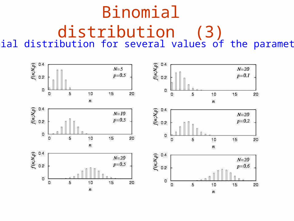
Binomial distribution (3)Binomial distribution for several values of the parameters:

Poisson distributionConsider binomial n in the limit

→ n follows the Poisson distribution:

Uniform distributionConsider a continuous r.v. x with ∞ < x < ∞ . Uniform pdf is:

N.B. For any r.v. x with cumulative distribution F(x),y = F(x) is uniform in [0,1].

Exponential distributionThe exponential pdf for the continuous r.v. x is defined by:

Example: proper decay time t of an unstable particle

( = mean lifetime)

Lack of memory (unique to exponential):

Gaussian distributionThe Gaussian (normal) pdf for a continuous r.v. x is defined by:

Special case: = 0, 2 = 1 (‘standard Gaussian’):

(N.B. often , 2 denotemean, variance of anyr.v., not only Gaussian.)

If y ~ Gaussian with , 2, then x = (y ) / follows (x).

Gaussian pdf and the Central Limit TheoremThe Gaussian pdf is so useful because almost any randomvariable that is a sum of a large number of small contributionsfollows it. This follows from the Central Limit Theorem:

For n independent r.v.s xi with finite variances i2, otherwise

arbitrary pdfs, consider the sum

Measurement errors are often the sum of many contributions, so frequently measured values can be treated as Gaussian r.v.s.

In the limit n → ∞, y is a Gaussian r.v. with

Chi-square (2) distribution

The chi-square pdf for the continuous r.v. z (z ≥ 0) is defined by

n = 1, 2, ... = number of ‘degrees of freedom’ (dof)

For independent Gaussian xi, i = 1, ..., n, means i, variances i2,

follows 2 pdf with n dof.

Example: goodness-of-fit test variable especially in conjunctionwith method of least squares.

Cauchy (Breit-Wigner) distribution

The Breit-Wigner pdf for the continuous r.v. x is defined by

= 2, x0 = 0 is the Cauchy pdf.)

E[x] not well defined, V[x] →∞.

x0 = mode (most probable value)

= full width at half maximum

Example: mass of resonance particle, e.g. , K*, 0, ...

= decay rate (inverse of mean lifetime)

Beta distribution

Often used to represent pdf of continuous r.v. nonzero onlybetween finite limits.

Student's t distribution

= number of degrees of freedom (not necessarily integer)

= 1 gives Cauchy,

→ ∞ gives Gaussian.

Student's t distribution (2)

If x ~ Gaussian with = 0, 2 = 1, and

z ~ 2 with n degrees of freedom, then

t = x / (z/n)1/2 follows Student's t with = n.

This arises in problems where one forms the ratio of a sample mean to the sample standard deviation of Gaussian r.v.s.

The Student's t provides a bell-shaped pdf with adjustabletails, ranging from those of a Gaussian, which fall off veryquickly, (→ ∞, but in fact already very Gauss-like for = two dozen), to the very long-tailed Cauchy ( = 1).

Developed in 1908 by William Gosset, who worked underthe pseudonym "Student" for the Guinness Brewery.

Multivariate distributions

Outcome of experiment charac-

terized by several values, e.g. an

n-component vector, (x1, ... xn)

joint pdf

Normalization:

Marginal pdf

Sometimes we want only pdf of some (or one) of the components:

→ marginal pdf

x1, x2 independent if

i

Marginal pdf (2)

Marginal pdf ~ projection of joint pdf onto individual axes.

Conditional pdf

Sometimes we want to consider some components of joint pdf as constant. Recall conditional probability:

→ conditional pdfs:

Bayes’ theorem becomes:

Recall A, B independent if

→ x, y independent if

Covariance and correlation

Define covariance cov[x,y] (also use matrix notation Vxy) as

Correlation coefficient (dimensionless) defined as

If x, y, independent, i.e., , then

→ x and y, ‘uncorrelated’

N.B. converse not always true.

Correlation (cont.)

Multinomial distributionLike binomial but now m outcomes instead of two, probabilities are

For N trials we want the probability to obtain:

n1 of outcome 1,n2 of outcome 2,

nm of outcome m.

This is the multinomial distribution for

Multinomial distribution (2)Now consider outcome i as ‘success’, all others as ‘failure’.

→ all ni individually binomial with parameters N, pi

for all i

One can also find the covariance to be

Example: represents a histogram

with m bins, N total entries, all entries independent.

Multivariate Gaussian distribution

Multivariate Gaussian pdf for the vector

are column vectors, are transpose (row) vectors,

For n = 2 this is

where = cov[x1, x2]/(12) is the correlation coefficient.