University of WollongongResearch Online

University of Wollongong Thesis Collection University of Wollongong Thesis Collections

1998

The development of a generic electrochemicalsensing system for ion chromatographyDaniela Maria OngaratoUniversity of Wollongong

Research Online is the open access institutional repository for theUniversity of Wollongong. For further information contact the UOWLibrary: research-pubs@uow.edu.au

Recommended CitationOngarato, Daniela Maria, The development of a generic electrochemical sensing system for ion chromatography, Doctor of Philosophythesis, Department of Chemistry, University of Wollongong, 1998. http://ro.uow.edu.au/theses/1201

THE DEVELOPMENT OF A GENERIC ELECTROCHEMICAL SENSING SYSTEM FOR

ION CHROMATOGRAPHY

A thesis submitted in fulfilment of the

requirements for the award of the degree

DOCTOR OF PHILOSOPHY

from

The University of Wollongong

by

DANIELA MARIA ONGARATO, BSc (Hons).

Department of Chemistry

March, 1998

for m y mother

CERTIFICATE

I certify that this thesis has not already been submitted for any degree and is

not being submitted as part of candidature for a degree at any other

university or institution.

Signature of Candidate.

ACKNOWLEDGMENTS

M y first thanks must go to m y supervisor, Prof. Gordon Wallace for his enthusiasm, support and extraordinary patience over the years.

I am most grateful to Dr. Richard John (Griffíth University), Dr. Serge Kokot (Queensland University of Technology) and Mr. Tuan Anh Nguyen (University of Wollongong) for their willing guidance. The financial and technical support of the Dionex Corporation (USA) is also gratefully acknowledged.

My sincere thanks go to Dr. Olaf Reinhold (Defence Science and Technology Organisation), Steve Cooper, John Reay and Peter Sarakiniotis (University of Wollongong) for their invaluable technical advice and assistance.

I wish to express my gratitude to the staff and students of the Intelligent Polymer Research Institute for their help and fhendship over the years. Thanks to Richard John, Peter Innis, Norm Barisci, Trevor Lewis and Chee O n Too for proofreading.

I owe a very big thankyou to Louisa Willdin, Karin Maxwell, Kerry Gilmore, Peta Murray and Vicky Wallace for ali their good humour and unwaveríng fhendship and support through everything.

My final and biggest thanks go to my family. Especially to my mother, whose grace, kindness and strength could fill a million of these pages, and to w h o m this work is dedicated.

n

TABLE OF CONTENTS

CERTIFICATION I AC K N O W L E D G M E N T S II TABLE OF CONTENTS TH LIST OF PUBLICATIONS VIU LIST OF ABBREVIATIONS X ABSTRACT XII

CHAPTER 1 1 INTRODUCTION

1.1 Introduction 1

1.2 Artificial Sensing Systems 5 1.2.1 Applications and Advantages 5 1.2.2 The Sensors 6

1.3 Conducting Electroactive Polymers 8 1.3.1 The Dynamic Nature of Conducting Electroactive

Polymers. 9 1.3.2 Synthesis of CEPs 11 1.3.3 Conductivity of CEPs 13 1.3.4 CEP Sensors 16

1.4 Microelectrode Arrays 17

1.5 Electrochemical Techniques 19 1.5.1. Cyclic Voltammetry 19 1.5.2. Pulsed Amperometry 21

1.6 Multichannel Potentiostat and Data Acquisition 23

1.7 Chemometrics 1.7.1 Data Pre-Processing 1.7.2 Principal Components Analysis 1.7.2.1 Score-Score Plots and Biplots 1.7.3 Partial Least Squares Regression 1.7.3.1 Response Plots

24 26 27 28 30 32

III

1.8 Scope Of This Thesis 32

CHAPTER 2 35 EXPERIMENTAL PROCEDURES.

2.1

2.2

Electrochemical Methods 2.1.1 Polymer Synthesis 2.1.1.1 Reagents and Solutions 2.1.1.2 Instrumentation 2.1.1.3 Working Electrode Configurations 2.1.2 Polymer Characterisation 2.1.2.1 Reagents and Solutions 2.1.2.2 Instrumentation

Analytical Methods 2.2.1 Ion Chromatography/Flow Injection Analysis 2.2.1.1 Reagents and Solutions 2.2.1.2 Instrumentation

35 35 35 36 37 44 45 45

46 46 46 48

2.3 Multichannel Potentiostat, Control and Data Acquisition System. 50 2.3.1 Multichannel Potentiostat and Data Acquisition

Hardware 51 2.3.2 Data Acquisition Software 53 2.3.2.1 Data Processing Procedures. 54

2.4 Chemometric Procedures 56 2.4.1 Data Handling 56

CHAPTER 3 57 SYNTHESIS AND CHARACTERISATION OF POLYMER COATED ELECTRODES

3.1 Introduction 57

3.2 Experimental 58

3.3 Results and Discussion 58

IV

3.3.1 Polymer Deposition 56 3.3.1.1 The Nature Of Monomer And Counterion 5 9 3.3.1.2 The Concentration Of Monomer and/or

Counterion 60 3.3.1.3 Current Density 61 3.3.1.4 Effect of Electrode Size and Shape 62 3.3.2 Nafion Pre-treatment 66 3.3.3 Electrode Coverage and Morphology 73

3.4 Summary and Conclusions 76

C H A P T E R 4 78 SIGNAL GENERATION

4.1 Introduction 78

4.2 Experimental 79

4.3 Results and Discussion 79 4.3.1 Cyclic Voltammetry 79 4.3.2 Chronoamperometric Studies 84 4.3.2.1 Pulse Duration 87 4.3.2.2 Pulsed Potential Ranges 90 4.3.2.3 Polymer Composition 91 4.3.2.4 Kinetic Effects 92 4.3.3. Competition Effects 92 4.3.4. Polymer Stability in Suppressed Eluents 93

4.4 Summary and Conclusions 98

CHAPTER 5 99 BEHAVIOUR OF CEP SENSORS IN A FLOW CELL -DETECTION OF ANIONS AND CATIONS AFTER ION CHROMATOGRAPHY.

5.1 Introduction. 99

5.2 Experimental. 99

5.3 Results and Discussion. 100

5.3.1 Polymer Composition. 100 5.3.2 Electrochemical Parameters. 107 5.3.3 Current Sample Point. 108 5.3.4 Effect of Polymer Thickness on Selectivity

Behaviour 110 5.3.5 Sensor Performance. 114 5.3.5.1 Reproducibility. 114 5.3.5.2 Analytical Performance. 116

5.4 Summary and Conclusions. 121

CHAPTER 6 123 THE CHEMOMETRIC ANALYSIS OF CYCLIC VOLTAMMOGRAMS AND THE OPTIMISATION OF FLOW INJECTION ANALYSIS PARAMETERS USING PRINCIPAL COMPONENTS ANALYSIS.

6.1 Introduction 123

6.2 Experimental 124

6.3 Results and Discussion 125 6.3.1 Optimisation of Flow Injection Analysis Detection

Parameters 125 6.3.1.1 Raw FIA Data 125 6.3.1.2 Optimisation of Pulsed Detection Parameters 127 6.3.2 Cyclic Voltammetry 141 6.3.2.1 Visual Analysis of CVs 142 6.3.2.2 Principal Components Analysis of CVs 143 6.3.2.3 The PCA of CVs for the Prediction of Optimal

Electrochemical and Chemical Detection Parameters 146

6.4 Summary and Conclusions 151

CHAPTER 7 153 THE ANALYSIS OF POTASSIUM A N D M E T H Y L A M I N E MLXTURES

7.1 Introduction 153

vi

7.2 Experimental 153

7.3 Results and Discussion 155 7.3.1 Principal Components Analysis 155 7.3.2 Partial Least Squares Regression Analysis 156

7.4 Summary and Conclusions 160

CHAPTER 8 161 GENERAL CONCLUSIONS AND FUTURE W O R K

8.1 General Conclusions 161

8.2 Future Work 165

APPENDIX 166

Appendixl.l 166 Appendix2.1 167 Appendix2.2 168 Appendix3.1 170 Appendix3.2 171 Appendix3.3 173 Appendix5.1 174 Appendix 5.2 175 Appendix 5.3 176 Appendix 7.1 177

REFERENCES 178

VII

LIST OF PUBLICATIONS

PUBLICATIONS

D.M. Ongarato, R. John and G.G. Wallace "Development of a Conducting Polymer-based Microelectrode Array Detection System." Electroanalysis, 8(7):623-629, 1996 Jul.

J.N. Barisci, A. Lawal, D.M. Ongarato, A. Partridge and G.G. Wallace. "Electroformation of Polymer Devices and Structures." Proceedings of the SPE 55th Annual Technical Conference and Exhibits, A N T E C '97, 1472-1475.

D.M. Ongarato, Tuan Anh Nguyen and G.G. Wallace "The Use of Chronoamperograms in FIA for the Detection of Potassium and Methylamine Using a Conducting Polymer-based Detection System." (Submitted).

D.M. Ongarato, Serge Kokot, Tuan Anh Nguyen and G.G. Wallace "The Selection of Pulsed Amperometric Detection Parameters for a Conducting Polymer-based Sensor Array Using Principal Components Analysis." (Submitted).

D.M. Ongarato, Serge Kokot, Tuan Anh Nguyen and G.G. Wallace "The Use of Cyclic Voltammetry and Principal Components Analysis to Tune the Selectivity of a Conducting Polymer Sensor Array" (Submitted).

D.M. Ongarato, and G.G. Wallace "The Analytical Performance Of A Conducting Polymer-Based Microarray Detection System - Implications For Signal Generation." (In preparation).

D.M. Ongarato, Serge Kokot, Tuan Anh Nguyen and G.G. Wallace "The Determination Of Potassium And Methylamine Peak Integrity Using A Conducting Electroactive Polymer-Based Sensing System." (In preparation)

VIII

P A P E R S P R E S E N T E D

"Novel Sensory Systems Based on Conducting Polymers." Presented February 1997 at the lOth Australasian Electrochemistry Conference, Gold Coast, Austrália,

"The Electronic Nose - Will it Sniff Underwater?" Presented June 1966 at the 4th N e w Zealand Symposium on Chemical And Biosensors, Christchurch, N e w Zealand.

"Conducting Polymer Coated Microelectrodes - A Tunable Detector for Ion Chromatography." Presented March 1995 at Pittcon 1995, N e w Orleans, U S A

"A Polymer Based Microarray Detection System." Presented March 1995 at Pittcon 1995, N e w Orleans, U S A

"A Polymer-Based Microelectrode Detection System." Presented December 1994 at the Royal Australian Chemical Institute Analytical Chemistry Group Research and Development Topics, Canberra, Austrália.

IX

LIST OF ABBREVIATIONS

A A" Ag/AgCI ASCII C +

°C CEP cm csp CV DAQ E Ei, E2 e" E E

r^red

FIA FMCA g hrs HPLC i I/O board iR K L MA M m mN min n nA PC PCA PED PLS

Ampere Anion Silver/silver chloride reference electrode American standard code for information interchan Cation

degrees Celsius Conducting electroactive polymer Centimetre Current sample point Cyclic voltammetry Data acquisition Potential switching potentials Electron Applied potential Oxidation potential Reduction potential Flow injection analysis Ferrocene monocarboxylic acid Gram hours High performance liquid chromatography Current Input/output board or card Ohmic drop Potassium Litre Methylamine Molar Milli (prefíx) Millinolar Minutes Number of electrons Nanoampere Principal component(s) Principal components analysis Pulsed electrochemical detector Partia! least squares regression analysis

PP PP/Cl PP/DS PP/MSA PP/NDSA PP/NO3 PP/PSS PP/PTS PP/SO4 PP/Tir ppb ppm QCM R S SAW see SEM t

T Tx Ty

u V X Y

Polypyrrole polypyrrole/chloride poíypyrrole/dodecylsulphate polypyrrole/mesitylene sulphonate polypyrrole/naphthalene disulphonic acid polypyrrole/nitrate polypyrrole/poly(4-styrenesulphonate) polypyrrole/para toluene sulphonate polypyrrole/sulphate polypyrrole/tiron parts per billion parts per million Quartz crystal microbalance Resistance Siemens Surface acoustic wave Seconds Scanning electron microscopy Time Pulse period Latent variable for matrix X Latent variable for matrix Y Micro (prefíx) Volt(s) Independent variable data matrix Dependent variable data matrix

XI

ABSTRACT

A generic electrochemical sensing system for ion chromatography has been

developed. The system comprised of a number of hardware and software

components. These included photolithographically produced,

microelectrodes coated with conducting electroactive polymer (CEP) as

sensing elements, with multichannel data acquisition, signal processing and

data analysis elements. This system was applied to pulsed amperometric

detection of a range of anions and cations after their separation by ion

chromatography. In conjunction with chemometric data analysis, the

problem of potassium (K) and methylamine ( M A ) peak integrity was

addressed. In the course of this work, the sensor array was effectively tuned

by the principal components analysis (PCA) of K and M A flow injection

analysis (FIA) data. In this way, the optimal chemical and electrochemical

detection parameters were identifíed as being: PP/Cl, PP/MSA, PP/PSS

(between switching potentials of-0.75V and -0.25V vs Ag/AgCI reference

electrode), PP/DS and PP/Tir (between switching potentials of-0.95V and

-0.45V vs Ag/AgCI reference electrode).

Analysis of score and biplots generated by the PCA of CV data represents a

fast and experimentally simpler method of tuning sensor selectivity. This

was a novel treatment of C V data and certainly the first reported for the

identification of pulsed detection parameters for FIA. This method

produced results which were in agreement with those obtained with the FIA

data.

xn

The optimised array, in conjunction with partial least squares (PLS)

regression analysis, was able to discriminate between purê and impure K

and M A peaks of up to 5 % M A impurity in K or to 2 0 % K impurity in M A .

Through this work, the flexibility offered to the system by post-acquisition

data manipulation was demonstrated. The use of current responses gathered

over whole pulses rather than discrete current sample points was shown to

be an effective strategy in this application.

The analytical performance of the CEP sensors to a range of electroinactive

anions and cations did not compare favourably to conductivity detection.

Calibration curves revealed that the C E P sensors are subject to polymer

"saturation" effects, in that the analytical signal did not increase indefínitely

with analyte concentration. This, along with sensitivity data for polymers

and conductivity detection, was evidence that the C E P responses were not

dominated by the change in solution conductivity.

x m

Chapter 1

CHAPTER 1

INTRODUCTION

1.1 INTRODUCTION

It is certain that most of us take for granted the sensor arrays we are

born with.

We are so concerned with the substance of our surroundings, that we

rarely contemplate the means through which this universe of sight,

sound, smell, taste and touch is experienced. And yet our senses,

coupled with our intelligence are what allow us to detect, recognise,

and respond to the multitude of physical and chemical variations w e

are exposed to every second of our lives. Therefore our senses (and

our intelligence) determine how successfully w e negotiate through life

itself.

Why are natural sensing systems so good?

What makes them so adaptive and universal?

Can we create a sensing system to equal or even surpass those which

have had the benefít of perhaps a billion years of evolution?

The nose and tongue - the body's natural chemical sensors - are

obvious sources of inspiration for those seeking to develop advanced

synthetic chemical sensing systems. They contain arrays of various

types of independem sensing elements (chemoreceptors) that work in

Chapter 1

parallel to rapidly and sensitively detect chemicals in vapour or liquid

state respectively. While the sensory elements are non-specific (ie

therefore able to detect a wide range of tastes or smells), each element

has a different selectivity (they will respond differently from each

other to the same substance). In this way a "fingerprint" response is

generated by the sensor array that is unique to the substance being

monitored.

The generation of "fingerprint" patterns by the sensor arrays represents

the first of two significant features of natural sensing systems. The

second feature is that the array is linked to an intelligence device that

acts as a pattern receiver, interpreter and recorder. That is, upon its

transmission, a signal "fingerprint" is registered, processed, identifíed

and then learned and remembered by an organic brain. A limited

quantitation capability does exist, since a judgement on the strength

(weak, strong, etc) of the taste or odour is possible.

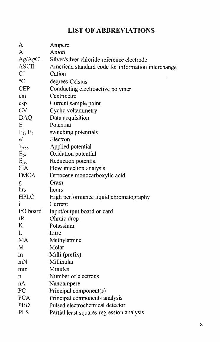
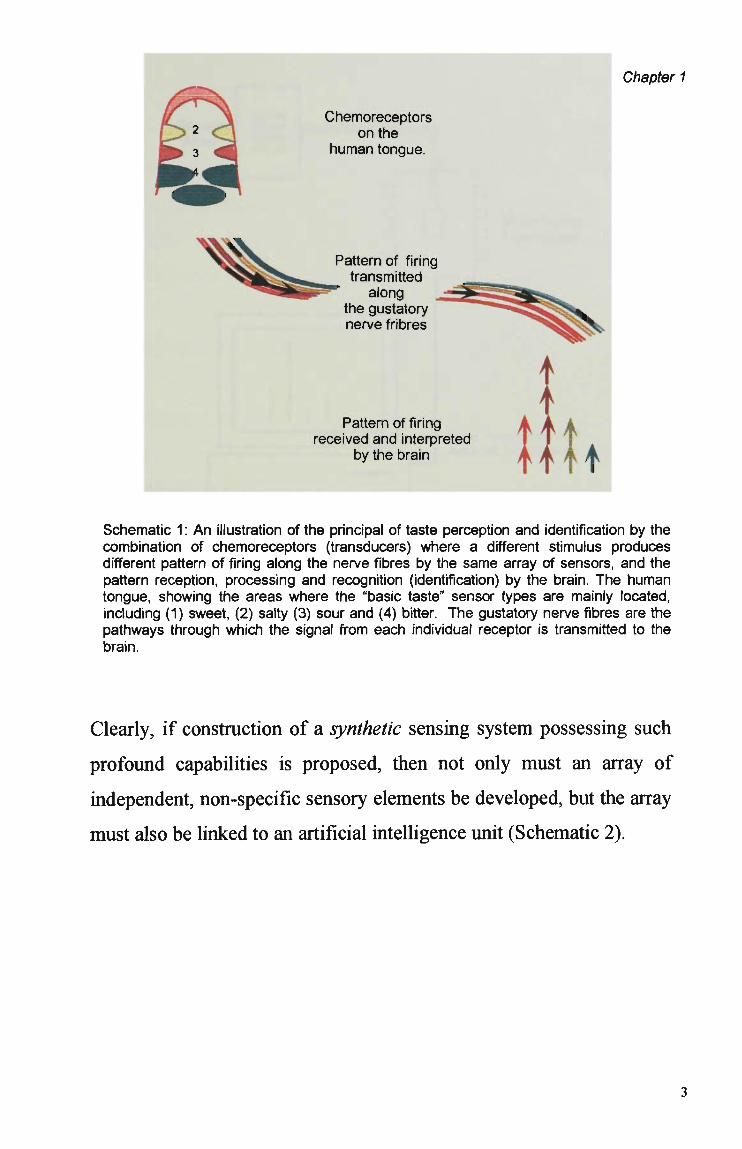
A simplified representation of the mammalian sensing system for

aqueous systems (the sense of taste) is shown in Schematic 1.

This multi-dimensional approach, an elegant yet supremely functional

biological architecture, explains h o w the relatively small number of

sensory element types contained within these organs are able to

discriminate between an almost endless and diverse range of tastes.

The system is so effective that of the many thousands of tastes and

smells encountered in a lifetime, one m a y be identifíed many years

after an initial (and sometimes solitary) sensing experience.

2

Chapter 1

Chemoreceptors on the

human tongue.

Pattern of firing transmitted

along the gustatory nerve fribres

Pattern of firing received and interpreted

by the brain

Schematic 1: An illustration of the principal of taste perception and identification by the combination of chemoreceptors (transducers) where a different stimulus produces different pattern of firing along the nerve fibres by the same array of sensors, and the pattern reception, processing and recognition (identification) by the brain. The human tongue, showing the áreas where the "basic taste" sensor types are mainly located, including (1) sweet, (2) salty (3) sour and (4) bitter. The gustatory nerve fibres are the pathways through which the signal from each individual receptor is transmitted to the brain.

Clearly, if construction of a synthetic sensing system possessing such

profound capabilities is proposed, then not only must an array of

independent, non-specific sensory elements be developed, but the array

must also be linked to an artificial intelligence unit (Schematic 2).

3

Sensor Array

c c

l i

I I

Chapter 1

Multichannel Potentiostat.

Data Acquisition and Artificial Intelligence.

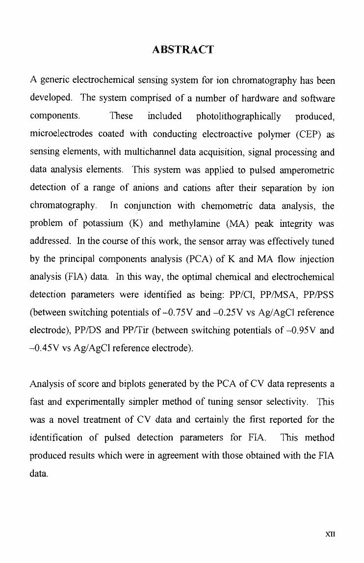
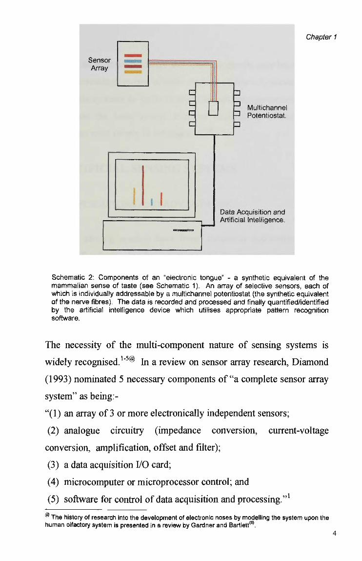
Schematic 2: Components of an "electronic tongue" - a synthetic equivalent of the mammalian sense of taste (see Schematic 1). An array of selective sensors, each of which is individually addressable by a multichannel potentiostat (the synthetic equivalent of the nerve fibres). The data is recorded and processed and finally quantified/identified by the artificial intelligence device which utilises appropriate pattern recognition software.

The necessity of the multi-component nature of sensing systems is

widely recognised.1"5® In a review on sensor array research, Diamond

(1993) nominated 5 necessary components of "a complete sensor array

system" as being:-

"(1) an array of 3 or more electronically independent sensors;

(2) analogue circuitry (impedance conversion, current-voltage

conversion, amplification, offset and filter);

(3) a data acquisition I/O card;

(4) microcomputer or microprocessor control; and

(5) software for control of data acquisition and processing."1

® The history of research into the development of electronic noses by modelling the system upon the human olfactory system is presented in a review by Gardner and Bartlett<6).

Chapter 1

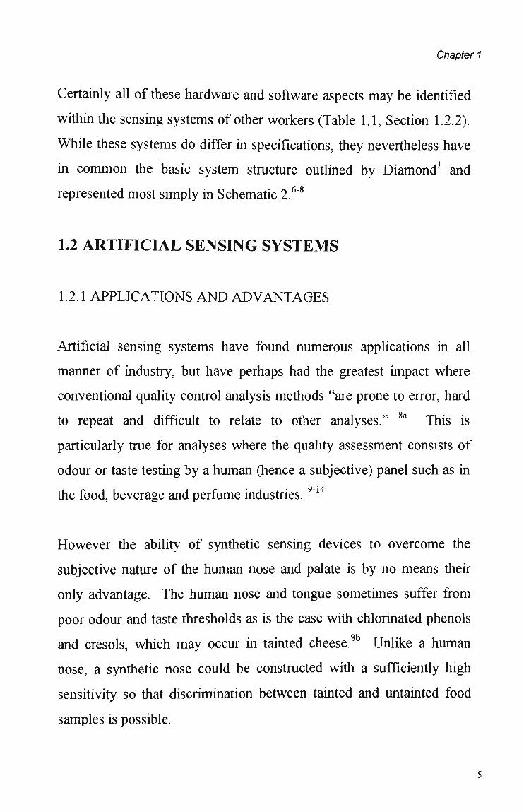
Certainly ali of these hardware and software aspects may be identifíed

within the sensing systems of other workers (Table 1.1, Section 1.2.2).

While these systems do differ in specifícatíons, they nevertheless have

in common the basic system structure outlined by Diamond1 and

represented most simply in Schematic 2.6"8

1.2 ARTIFICIAL SENSING SYSTEMS

1.2.1 APPLICATIONS AND ADVANTAGES

Artificial sensing systems have found numerous applications in ali

manner of industry, but have perhaps had the greatest impact where

conventional quality control analysis methods "are prone to error, hard

to repeat and difficult to relate to other analyses." 8a This is

particularly true for analyses where the quality assessment consists of

odour or taste testing by a human (hence a subjective) panei such as in

the food, beverage and perfume industries.9"14

However the ability of synthetic sensing devices to overcome the

subjective nature of the human nose and palate is by no means their

only advantage. The human nose and tongue sometimes suffer from

poor odour and taste thresholds as is the case with chlorinated phenols

and cresols, which may occur in tainted cheese.8b Unlike a human

nose, a synthetic nose could be constructed with a sufficiently high

sensitivity so that discrimination between tainted and untainted food

samples is possible.

5

Chapter 1

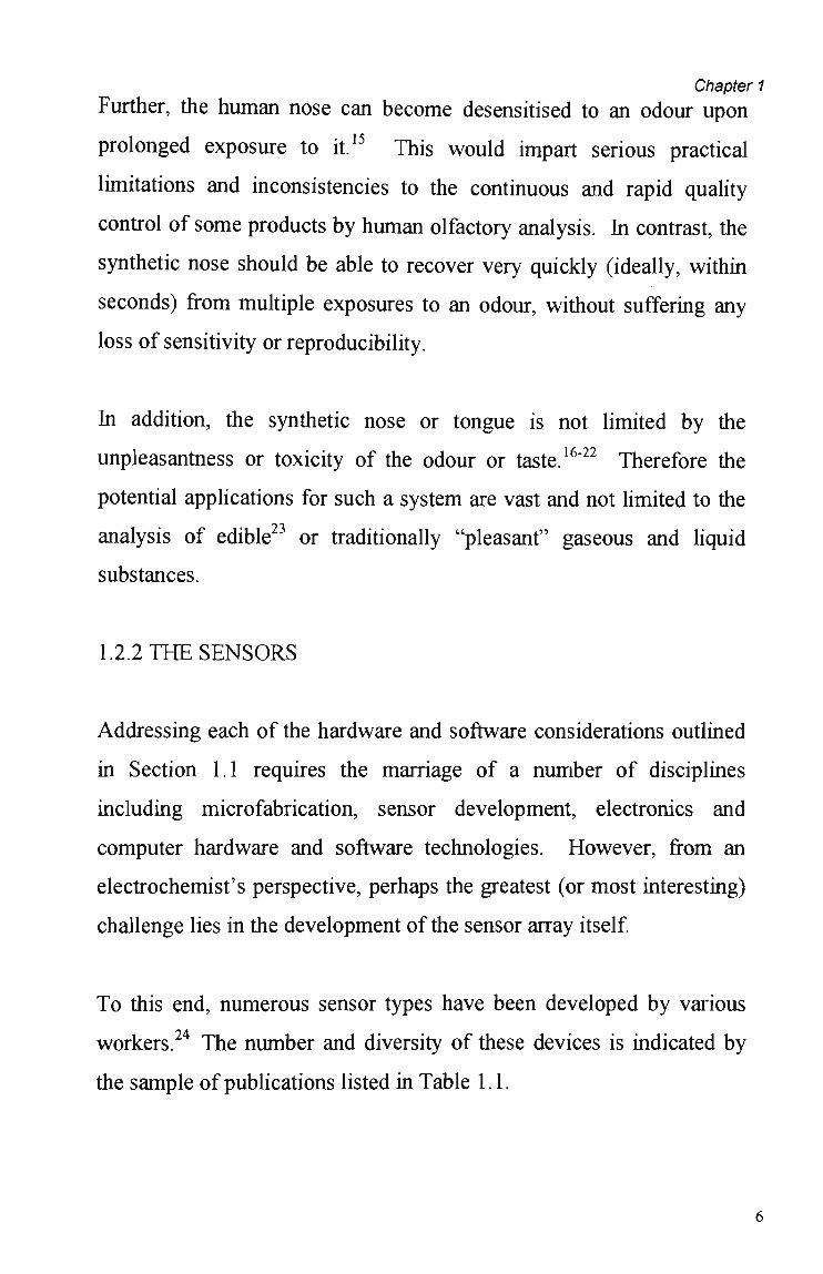
Further, the human nose can become desensitised to an odour upon

prolonged exposure to it.15 This would impart serious practical

limitations and inconsistencies to the continuous and rapid quality

control of some products by human olfactory analysis. In contrast, the

synthetic nose should be able to recover very quickly (ideally, within

seconds) from multiple exposures to an odour, without suffering any

loss of sensitivity or reproducibility.

In addition, the synthetic nose or tongue is not limited by the

unpleasantness or toxicity of the odour or taste.16"22 Therefore the

potential applications for such a system are vast and not limited to the

analysis of edible or traditionally "pleasant" gaseous and liquid

substances.

1.2.2 THE SENSORS

Addressing each of the hardware and software considerations outlined

in Section 1.1 requires the marriage of a number of disciplines

including microfabrication, sensor development, electronics and

computer hardware and software technologies. However, from an

electrochemisfs perspective, perhaps the greatest (or most interesting)

challenge lies in the development of the sensor array itself.

To this end, numerous sensor types have been developed by various

workers.24 The number and diversity of these devices is indicated by

the sample of publications listed in Table 1.1.

6

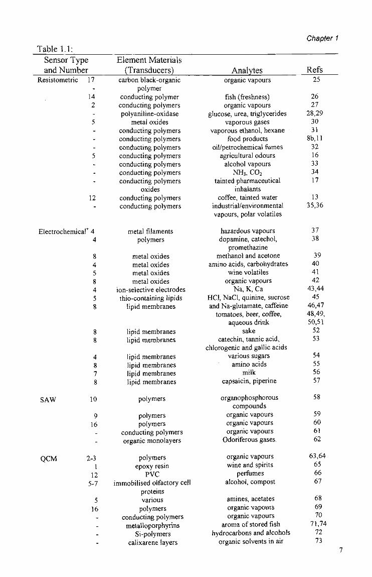
Table 1.1: Chapter 1

Sensor Type and Number

Resistometric 17 -

14 2 -

5 ---

5 ---

12 "

Electrochemicar 4 4

8 4 5 8 4 5 8

8 8

4 8 7 8

SAW 10

9 16 .

-

QCM 2-3 1 12 5-7

5 16 -.

-

-

Element Materials (Transducers)

carbon black-organic polymer

conducting polymer conducting polymers polyaniline-oxidase

metal oxides conducting polymers conducting polymers conducting polymers conducting polymers conducting polymers conducting polymers conducting polymers

oxides conducting polymers conducting polymers

metal fílaments polymers

metal oxides metal oxides metal oxides metal oxides

ion-selective electrodes thio-containing lipids

lipid membranes

lipid membranes lipid membranes

lipid membranes lipid membranes lipid membranes lipid membranes

polymers

polymers polymers

conducting polymers organic monolayers

polymers epoxy resin

PVC immobilised olfactory cell

proteins various polymers

conducting polymers metaUoporphyrins

Si-polymers calixarene layers

Analytes organic vapours

fish (freshness) organic vapours

glucose, urea, triglycerides vaporous gases

vaporous ethanol, hexane food products

oil/petrochemical fumes agricultural odours alcohol vapours

N H 3 , C 0 2

tainted pharmaceutical inhalants

coffee, tainted water industrial/environmental vapours, polar volatiles

hazardous vapours dopamine, catechol,

promethazine methanol and acetone

amino acids, carbohydrates wine volatiles organic vapours

Na, K, Ca HCI, NaCl, quinine, sucrose and Na-glutamate, caffeine

tomatoes, beer, coffee, aqueous drink

sake catechin, tannic acid,

chlorogenic and gallic acids various sugars amino acids

milk capsaicin, piperine

organophosphorous compounds

organic vapours organic vapours organic vapours

Odoriferous gases

organic vapours wine and spirits

perfumes alcohol, compost

amines, acetates organic vapours organic vapours

aroma of stored fish hydrocarbons and alcohols

organic solvents in air

Refs 25

26 27

28,29

30 31

8b, 11

32 16 33 34 17

13 35,36

37 38

39 40 41 42

43,44

45 46,47 48,49, 50,51

52 53

54 55 56 57

58

59 60 61 62

63,64

65 66 67

68 69 70

71,74

72 73

Chapter 1

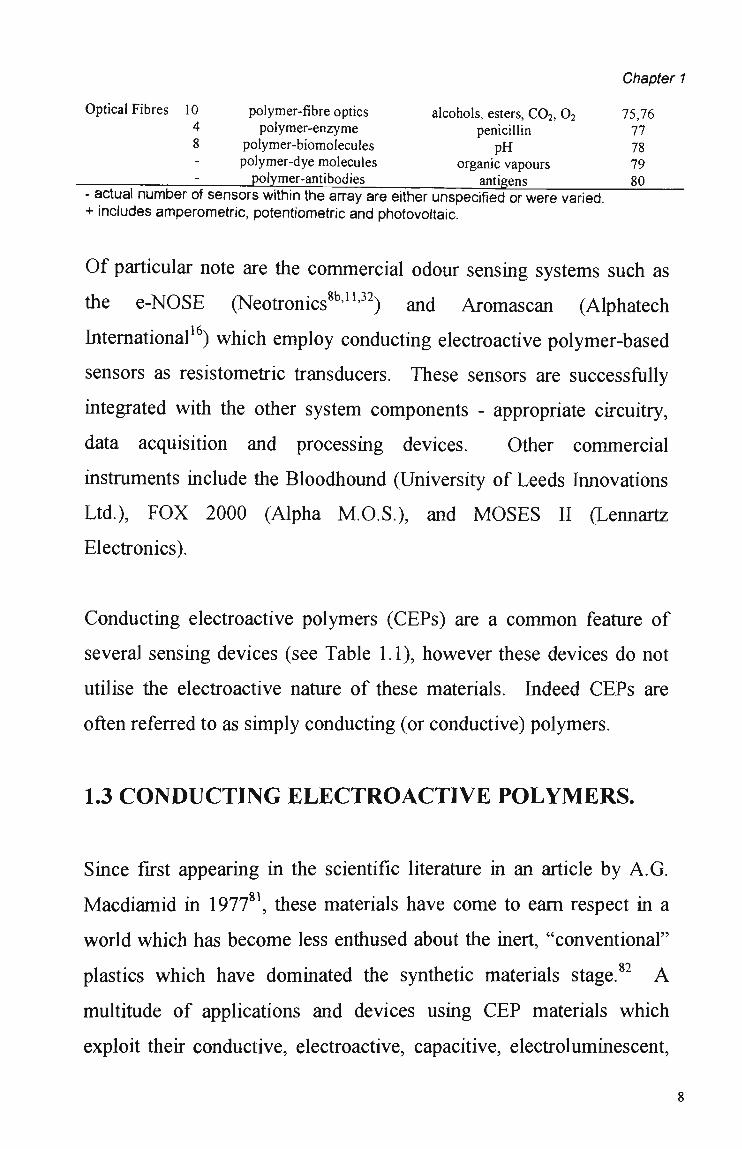
Optical Fibres 10 polymer-fibre optics alcohols, esters, C 0 2 , 0 2 75,76 4 polymer-enzyme penicillin 77 8 polymer-biomoíecules p H 78

polymer-dye molecules organic vapours 79 : polymer-antibodies antigens 80

- actual number of sensors within the array are either unspecified or were varied. + includes amperometric, potentiometric and photovoltaic.

Of particular note are the commercial odour sensing systems such as

the e-NOSE (Neotronics8b'n'32) and Aromascan (Alphatech

International6) which employ conducting electroactive polymer-based

sensors as resistometric transducers. These sensors are successfully

integrated with the other system components - appropriate circuitry,

data acquisition and processing devices. Other commercial

instruments include the Bloodhound (University of Leeds Innovations

Ltd.), F O X 2000 (Alpha M.O.S.), and M O S E S II (Lennartz

Electronics).

Conducting electroactive polymers (CEPs) are a common feature of

several sensing devices (see Table 1.1), however these devices do not

utilise the electroactive nature of these materiais. Indeed CEPs are

often referred to as simply conducting (or conductive) polymers.

1.3 CONDUCTING ELECTROACTIVE POLYMERS.

Since first appearing in the scientific literature in an article by A.G.

Macdiamid in 197781, these materiais have come to earn respect in a

world which has become less enthused about the inert, "conventional"

plastics which have dominated the synthetic materiais stage.82 A

multitude of applications and devices using C E P materiais which

exploit their conductive, electroactive, capacitive, electroluminescent,

8

Chapter 1

electromechanical or ion exchange properties n o w exist and research

into potential applications is ongoing83'84 (Table 1.2).

Table 1.2:

Application or Device

protective coatings and shielding timed drug delivery

rechargeable batteries and solid electrolyte capacitors

electronic display/electrochromic devices

sensing devices+ ion gate membrane applications

colloidal dispersions molecular, micro- and nanotechnology

artificial muscle

References and Reviews

85-89 91-94

90, 95-98

99, 100

16,26-28,31,101-104 105-109 110 89,90 111

+ also various references throughout the text and in Table 1.3.

The most well known members of this unique class of materiais

include polyacetylene and the polyheterocyclics polythiophene,

polyaniline and polypyrrole, or derivatives of the respective

monomers.112 The utility of these materiais can be largely attributed to

their dynamic electrical and chemical properties.

1.3.1 THE DYNAMIC NATURE OF CONDUCTING POLYMERS

Being an electroactive material, the polymer backbone can readily

exist in either an oxidised or a reduced state, possessing a positive or a

neutral charge respectively.

When oxidised, the positive charge on the polymer backbone is

neutralised by the subsequent incorporation of anions from the

supporting electrolyte. Reduction of the polymer from this oxidised

(doped) state, removes the positive charge from the chain which in turn

9

Chapter 1

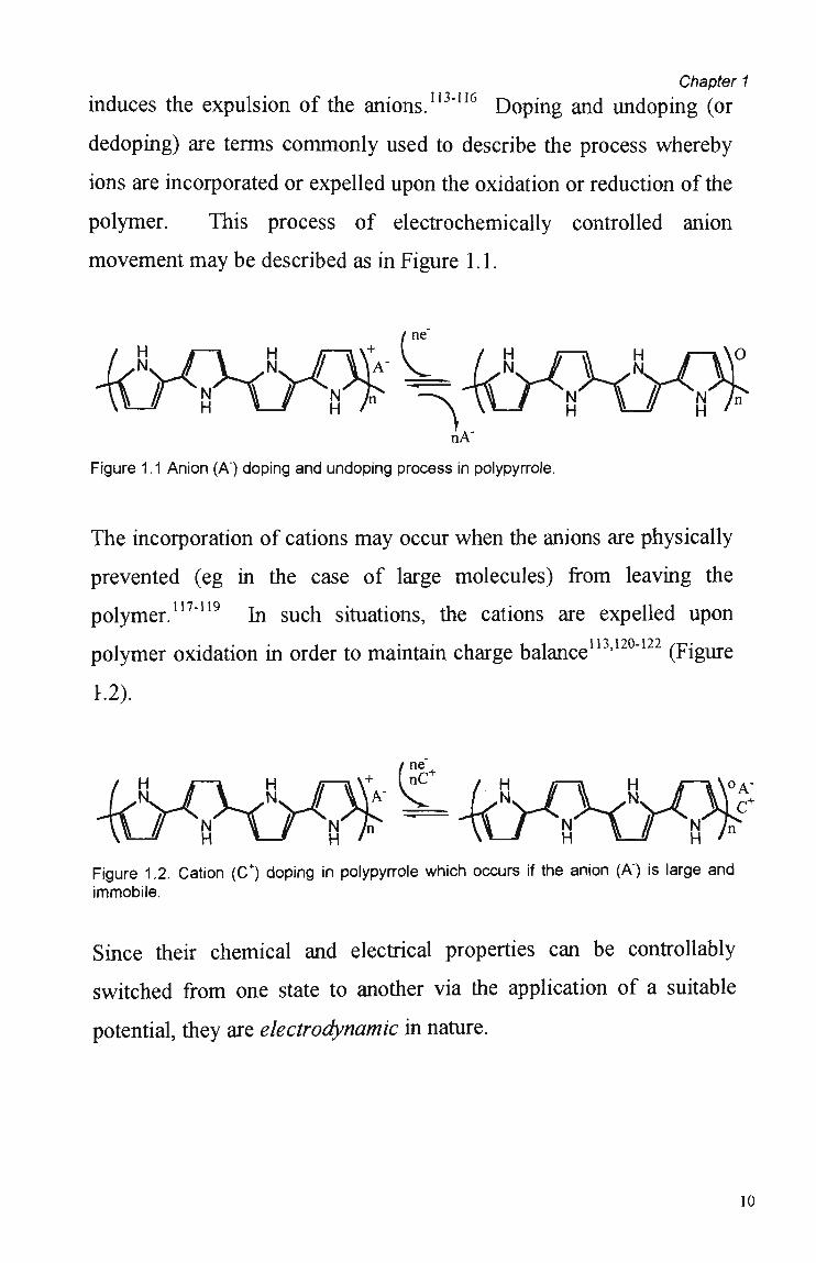
induces the expulsion of the anions.113"116 Doping and undoping (or

dedoping) are terms commonly used to describe the process whereby

ions are incorporated or expelled upon the oxidation or reduction of the

polymer. This process of electrochemically controlled anion

movement m a y be described as in Figure 1.1.

nA"

Figure 1.1 Anion (A') doping and undoping process in polypyrrole.

The incorporation of cations may occur when the anions are physically

prevented (eg in the case of large molecules) from leaving the

polymer.117"119 In such situations, the cations are expelled upon i i o i *)r\ i syy

polymer oxidation in order to maintain charge balance ' " (Figure

1.2).

/ne"+

Figure 1.2. Cation (C+) doping in polypyrrole which occurs if the anion (A") is large and immobile.

Since their chemical and electrical properties can be controllably

switched from one state to another via the application of a suitable

potential, they are electrodynamic in nature.

10

Chapter 1

1.3.2. S Y N T H E S I S O F CEPS.

One of the advantages of using CEP materiais is that they may be

electrochemically deposited directly to coat an electrode surface of

virtually any size or shape. Though chemical123"132 and

photochemical initiation of the polymerisation reaction is also

possible, the electrochemical synthesis route is often preferred for a

number of reasons:

(1) no chemical oxidants are required and so a wider variety of

counterions are available,

(2) greater control of polymer thickness is likely, since electrochemical

deposition parameters such as oxidation potential, current density

and deposition time m a y be accurately controlled,134"136

(3) films of greater mechanical strength and adhesion are generally "l *í A 1 *T 1 A f\

produced electrochemically, *

(4) the procedure is fast, simple and more reproducible than the

chemical alternative.141

The polymer forms as a film on the anode, as the radical monomer

cations produced are converted to dimers and finally to oligomers

which become insoluble as their chain length increases.112'142"151

"Subsequent deposition has a contribution from both electrode bound

polymer coupling with soluble radical species and from the

precipitation of low molar mass polymer chains which remain in

solution until the point where their solubility decreases." (Baker and

Reynolds, 1988142). Figure 1.3, reproduced from John and Wallace,

n

Chapter 1

1991 49 shows the steps involved in the electropolymerisation of

heterocyclics such as pyrrole.

The chemical composition of the polymer is determined by the

selection of both monomer and counterion in the polymerisation

solution. The chemical characteristics built into the polymer from

the time of synthesis have a profound impact in the use of these

materiais as sensors (Section 1.3.4).

12

Chapter 1 1. Monomer Oxidation

[A] [B]

2. Resonance forms

[C] [D] [E]

3. Radical - radical coupling

4. Chain propogation

<Y® -{yÇ-

Figure 1.3 Electropolymerisation of heterocyclics such as pyrrole (reproduced from ref. 149).

1.3.3. CONDUCTIVITY OF CEPS

These polymers are poor conductors of electricity when reduced.82 It is

the charged nature of the polymer backbone which establishes the

Chapter 1

degree and freedom of electron movement within the polymer, and

hence which makes them electrically conductive. Polymer

conductivity has been explained by the formation of polarons and

bipolarons within the polymer.153

A polaron is the positive charge and subsequent local distortion of the

lattice which arises because of the oxidation of the polymer (to its

doped form). W h e n a further electron is removed (during high doping)

a bipolaron is formed, since this is more energetically favourable than

the formation of two polarons near to each other.153

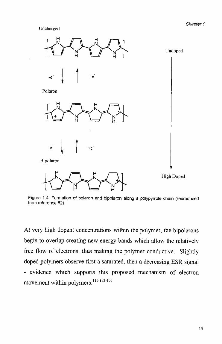
Figure 1.4 shows how the formation of the polaron and/or bipolaron

involves the shifting of carbon-carbon double and single bonds.

Since the polaron includes a radical cation, it has a spin of 1/2.

Bipolarons (dications), however are spinless. Electron Spin Resonance

(ESR) measurements confirm that at high dopant leveis the charge

carriers are spinless and therefore must be bipolarons.

14

-e

Polaron

r H

Bipolaron

+e

+e

Chapter 1

Undoped

High Doped

Figure 1.4: Formation of polaron and bipolaron along a polypyrrole chain (reproduced from reference 82)

At very high dopant concentrations within the polymer, the bipolarons

begin to overlap creating new energy bands which allow the relatively

free flow of electrons, thus making the polymer conductive. Slightly

doped polymers observe first a saturated, then a decreasing E S R signal

- evidence which supports this proposed mechanism of electron

movement within polymers.116'153"155

15

1.3.4. CEP SENSORS. Chapter 1

The notion of creating sensors based upon polymer materiais is not a

new one. Indeed, nature has been using proteins, polymers constructed

from amino acid building blocks, in biological sensors for millions of

years. In a way, conducting electroactive polymers (CEPs) might be

thought of as a kind of synthetic equivalent to biological polymers, in

that they m a y potentially exhibit similar molecular recognition and

chemical and electrochemical data transmission (transducing)

capabilities as those of some proteins.156

The molecular recognition capabilities of CEP materiais arise from the

different molecular interactions which occur upon exposure of these

materiais to both chemical and electrochemical stimuli. The nature

and extent of these interactions with the target analyte depends to a

large degree on the counterion contained within the polymer matrix.

For example, immobilising specific bioactive molecules into a

conducting matrix can create a sensor with inherent bio-specificity.

165 Exploiting this principie of mutual polymer/counterion/analyte

affinities has resulted in the successful polymer-based detection of a

range of analytes. In a recent review by Barisci, Conn and Wallace166

CEP-based sensing devices were categorised into three basic types;

amperometric, resistometric and potentiometric (Table 1.3).

16

Table 1.3 Chapter 1

C E P Sensor Type Analyte References

Amperometric proteins and biomaterials 101,102,158-163,167 various simple anions and 168-175

cations metal ions 176,177 ascorbate 178-180 pesticides 181

Resistometric ammonia, hydrazine 33,182 various gas vapours 16,26,27,31,71,183-185

Potentiometric chloride 186 ascorbic acid, dopamine 187,167

Each type of sensor utilises the dynamic chemical and electrical

properties of C E P materiais.

1.4. MICROELECTRODE ARRAYS

If conducting electroactive polymers are the building blocks of the

sensing device, then the microarray electrodes are the foundation.

A number of different types of sensing elements have been mentioned

(Table 1.1), including chemically modified optical fibres, surface

acoustic wave sensors ( S A W ) , quartz crystals used in the quartz crystal

microbalance ( Q C M ) as well as more conventional (metal) electrodes.

The sensing element type is determined by the nature of the signal that

is extracted and then measured (eg changes in oscillation frequency,

current flow, or some optical property, etc).24 In order to monitor the

current which flows as a result of the electrical (or chemical)

perturbation of CEPs in the presence of an analyte, simple electrode

substrates (eg, gold or platinum lines or discs) are adequate.

17

Chapter 1

These most simple and straightforward of array elements can be

constructed in a multitude of configurations and sizes and may

therefore be custom designed to suit a particular application. This is

particularly true of photolithography, a microsensor synthesis

technique in which metal (eg gold or platinum) patterns are

"developed" onto a substrate, most commonly glass or oxidised silicon

wafers102'188"192 (see Figure 2.4, Section 2.1.1.3). This is of tremendous

importance when miniaturisation is desirable and/or when multiple

elements are required.

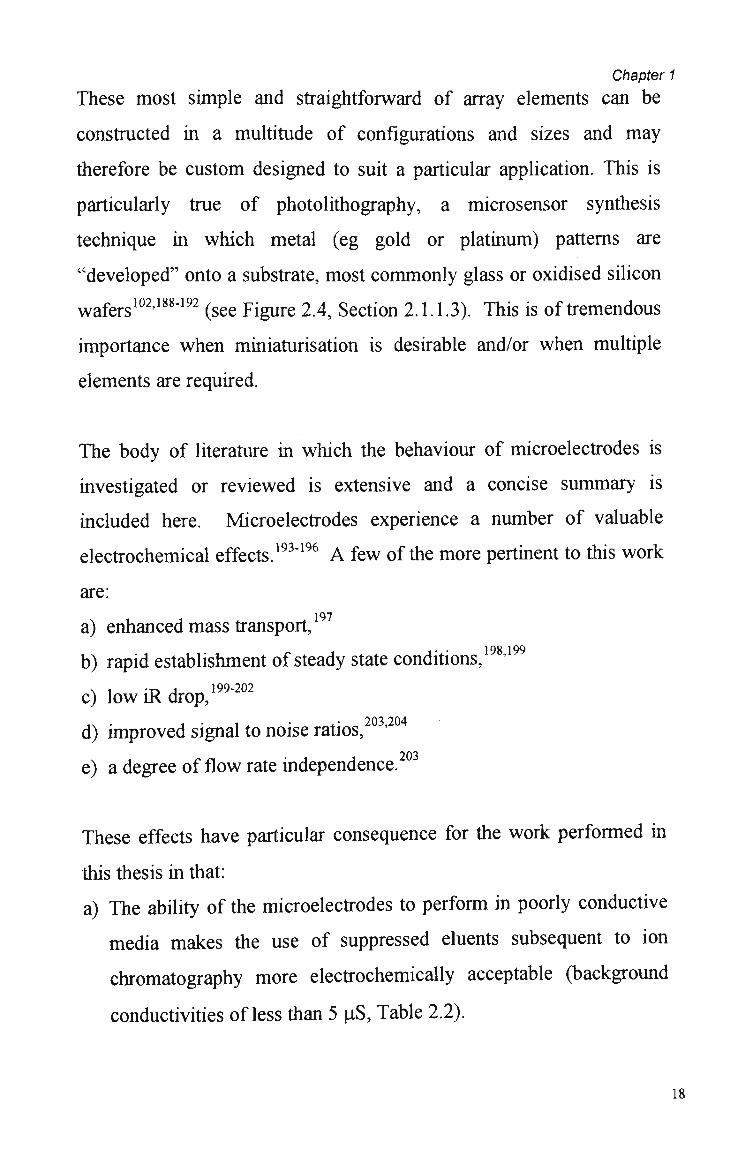
The body of literature in which the behaviour of microelectrodes is

investigated or reviewed is extensive and a concise summary is

included here. Microelectrodes experience a number of valuable

electrochemical effects.193"196 A few of the more pertinent to this work

are: 197

a) enhanced mass transport, • 198 199

b) rapid establishmentof steady state conditions, • c) low iR drop,199-202

203 204

d) improved signal to noise ratios, ' 203

e) a degree of flow rate independence.

These effects have particular consequence for the work performed in

this thesis in that:

a) The ability of the microelectrodes to perform in poorly conductive

media makes the use of suppressed eluents subsequent to ion

chromatography more electrochemically acceptable (background

conductivities of less than 5 uS, Table 2.2).

18

Chapter 1

b) The enhanced signal to noise ratio should lower the detection limits

achievable.174

c) The reduced dependence of the current response on flow rate is a

desirable property for detectors used with chromatographic or flow

injection analysis (FIA) applications.

1.5 ELECTROCHEMICAL TECHNIQUES

1.5.1 CYCLIC VOLTAMMETRY.

Cyclic voltammetry (CV) is one of the most useful electrochemical

characterisation techniques and can aid in the understanding and

appreciation of the electrochemical processes occurring at an electrode.

This is certainly true of the ion exchange processes which occur upon

electrochemical stimulation of C E P films in a supporting electrolyte.

C V experiments are fast, non-destructive, versatile and easy to perform

with electrodes of virtually any size or shape, but perhaps the most

important advantage of this technique is that the in-situ study of the

dynamic electrochemical behaviour of CEPs is possible.

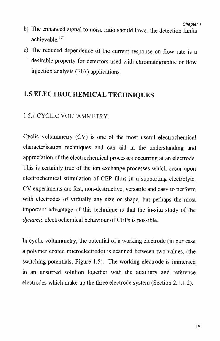
In cyclic voltammetry, the potential of a working electrode (in our case

a polymer coated microelectrode) is scanned between two values, (the

switching potentials, Figure 1.5). The working electrode is immersed

in an unstirred solution together with the auxiliary and reference

electrodes which make up the three electrode system (Section 2.1.1.2).

19

Chapter 1

> A c o

> Time

Figure 1.5: Scanned potential waveform in cyclic voltammetry (CV). E, and E 2 are the switching potentials

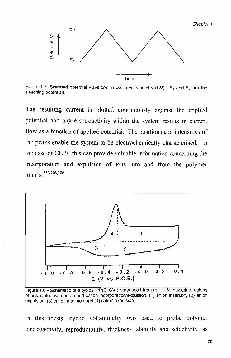
The resulting current is plotted continuously against the applied

potential and any electroactivity within the system results in current

flow as a function of applied potential. The positions and intensities of

the peaks enable the system to be electrochemically characterised. In

the case of CEPs, this can provide valuable information concerning the

incorporation and expulsion of ions into and from the polymer

matrix."3^2 0 6

Figure 1.6 - Schematic of a typical PP/Cl C V (reproduced from ref. 113) indicating regions of associated with anion and cation incorporation/expulsion: (1) anion insertion, (2) anion expulsion, (3) cation insertion and (4) cation expulsion.

In this thesis, cyclic voltammetry was used to probe polymer

electroactivity, reproducibility, thickness, stability and selectivity, as

20

Chapter 1

well as the "micro" (ie the mass transfer) properties of the array electrodes.

1.5.2. PULSED AMPEROMETRY

Like the scanned potential waveform, the pulsed waveform (illustrated

in Figure 1.7) can also be used to characterise polymer/electrolyte

interactions. The rapid manipulation of polymer redox state can be

particularly useful to probe the kinetics of anion and cation movement

which occurs with various polymer/electrolyte combinations (see

chronoamperograms in Figure 1.8).

E2 I [ I

El I

< > T

Figure 1.7: Pulsed Applied Potential Waveform. E1 and E2 are the switching potentials. The pulse period is here denoted T.

21

Chapter 1

60x10

40 -

= 20 -I

«D

CJ

0 -

-20 -

40 -

PP/TlRON

0.0 I

1.0 2.0

Time( seconds)

3.0 l

4.0

Figure 1.8: Examples of the chronoamperometric responses of three different polypyrrole (PP) coated electrodes: PP/Tiron, PP/DS and PP/MSA in 10"4 M NaCl supporting electrolyte, where E, = -0.4 V and E 2 = 0.25 V.

As well as it's use in characterisation of polymer/electrolyte systems,

the pulsed potential waveform has proved most appropriate in

electrochemical detection methods.

Certainly one of the strengths of the pulsed waveform in

electrochemical detection scenarios is that it allows the electrochemical

renewal of the sensing surface. This was recognised by Ikariyama and

Heineman69 w h o were the first to use the doping/dedoping nature of

C E P coated electrodes as sensors in the flow injection analysis (FIA)

of such electroinactive anions as phosphate, carbonate and acetate. In

this case, the pulsed potential waveform regenerated the electrode (by

inducing the expulsion of anions from the polymer matrix via

application of a reducing potential), between successive exposures of

the oxidised polymer to analyte sample plugs.

22

Chapter 1

The use of pulsed potential waveforms to induce controlled

anion/cation movement throughout the polymer matrix is the key to the

success of C E P coated sensors for use in the liquid phase. This type of

signal generation waveform allows the chemical, electrochemical and

kinetic selectivity aspects of the polymer/electrolyte interactions to be

exploited in electrochemical FIA or chromatography detectors. The

principies behind C E P sensor signal generation is the topic of Chapter

4, where the origins of the various selectivity aspects are examined.

1.6. MULTICHANNEL POTENTIOSTAT AND DATA

ACQUISITION.

The olfactory and gustatory cells in the nose and tongue respectively

are connected to a series of nerve fibres which effectively

communicate the responses of each of the cells to the brain. The

synthetic equivalent of those nerve fibres in electrochemical systems is

the multichannel potentiostat. This instrument, in conjunction with

control hardware and software would constitute the "analogue circuitry

(impedance conversion, current-voltage conversion, amplification,

offset and filter)... and microcomputer or microprocessor control"

aspects of "a complete sensor array system" identifíed by Diamond.1

The importance of having a low noise instrument capable of addressing

each element in the array independently and simultaneously has been

recognised by other workers.44'207*212 In addition the data acquisition

component must allow the simultaneous monitoring and recording of

data from many channels. This involves the utilisation of "a data

Chapter 1

acquisition I/O card (and) software for control of data acquisition and

processing".! Post-experiment data processing is also often required.

The instrument used in this work is described in some detail in Section

2.3.

1.7 CHEMOMETRICS

To develop a synthetic "sense", the data receiving, processing and

recording functions of an analogous organic brain may be performed

by a combination of computer hardware and software. Just as

important are the pattern recognition capabilities of the natural system

which must also be emulated in the synthetic approach. To this end, a

number of chemometric strategies are commonly employed in the

analysis of multivariate data which has been derived from various 37 213-221

sensor arrays. '

Chemometrics has been defined as the "discipline concerned with the

application of statistical and mathematical methods, as well as those

methods based on mathematical logic to chemistry",222 but this

succinct definition belies the scope of this truly multidisciplinary field.

Thousands of papers containing the results of chemometric analyses

are published every year from such varied áreas as chemical

engineering, as well as the analytical, environmental, biochemical and

medicai disciplines,215'222'224 where it is "used to extract valuable, but

often hidden, information from measurements."218

24

Chapter 1

These mathematical methods, grouped under the collective title of

pattern recognition (but one sub-branch of chemometrics) may

themselves be classified as being either parametric or nonparametric

(Figure 1.9). Parametric methods assume that the statistical

distribution of the data is known or can be estimated. Nonparametric

methods make no statistical assumptions about the data.

Experimental Design

Artificial Neural

Networks Non-Parametric

Chemometrics

Pattern Recognition

} f Preprocessing ( Factor Analysis) f Classification

T^—' u Hierarchial

- Mean Centering

- Standardisation

-Autoscaling

Normalisation

Double Centering

-PCA L Factor

Analysis Clustering

Process Optimisation

Parametric

Classification

Analysis

li Regression

Analysis

-SIMCA

*- Discriminant

Analysis (eg RDA)

-PCR

-PLS

-NPLS LACE

Figure 1.9: Summary (flow chart) of various pattern recognition methods. PCA = principal Components Analysis, SIMCA = Soft Independent Modelling of Class Analogy, RDA = Regularised Discriminant Analysis, PCR = Principal Components Regression, PLS = Partia! Least Squares Regression, NPLS = Non-linear Partial Least Squares Regression, ACE = Alternating Conditional Expectations.

Perhaps the most often used method in analysing multivariate data is

the "exploratory" (sometimes referred to as the display215) method of

principal component analysis (PCA, Section 1.7.2).

25

Chapter 1

1.7.1 D A T A P R E - P R O C E S S I N G

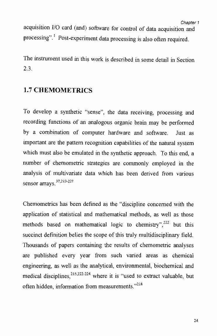
Autoscaling is perhaps the most common data pre-treatment procedure

actually consisting of two pre-processing methods - mean centering

and standardisation.

Mean centering is where the mean value of a column (ie the mean of a

variable) is subtracted from every value in that column. This

effectively centres the data around the origin of the coordinate system.

This is done to improve the ability of the principal component to

explain the variance in the data (see Section 1.7.2).

Standardisation is performed because many pattern recognition

methods are scale dependent. This is especially true if the variables

have different units (eg. variable 1 is (say) in grams, variable 2 in is

Amperes, variable 3 is in °C, and so on). To overcome this the

variables may be scaled so that each variable (ie each column in the

data matrix) has a variance of 1. This is done by dividing each value in

the column by the standard deviation of the column. "This variance

scaling makes ali coordinate axes have the same length, giving each

variable the same influence on the model."

The effect of autoscaling on raw data is illustrated in Figure 1.10 (an

example reproduced here from reference 226).

26

Chapter 1

B D

Figure 1.10: Data preprocessing. The data for each variable are represented by a variance bar and its center. (A) Most raw data look like this. (B) The result after mean-centering only. (C) The result after variance-scaling only. (D) The result after autoscaling

1.7.2 PRINCIPAL C O M P O N E N T S A N A L Y S I S (PCA).

PCA, also known as eigenanalysis, is a non-parametric, "unsupervised"

pattern recognition method because it lets "the data talk for themselves

without a priori models in mind".229 This makes it particularly suitable

for the initial "exploration" of a data set, where the aim is simply to

identify any inherent groupings or clusters within the data, as well as

outliers and any "structure" in the data in general. This is done by

analysis of the variance (amount of variation) within the data.

In PCA, multivariate data is reduced - the data matrix is expressed by

orthogonal principal components (PCs) which describe leveis of

variance in the data (Figure 1.11). In this way a few PCs can (usually)

express a large percentage of the variance, regardless of the number of

variables in the original data matrix.

27

Chapter 1

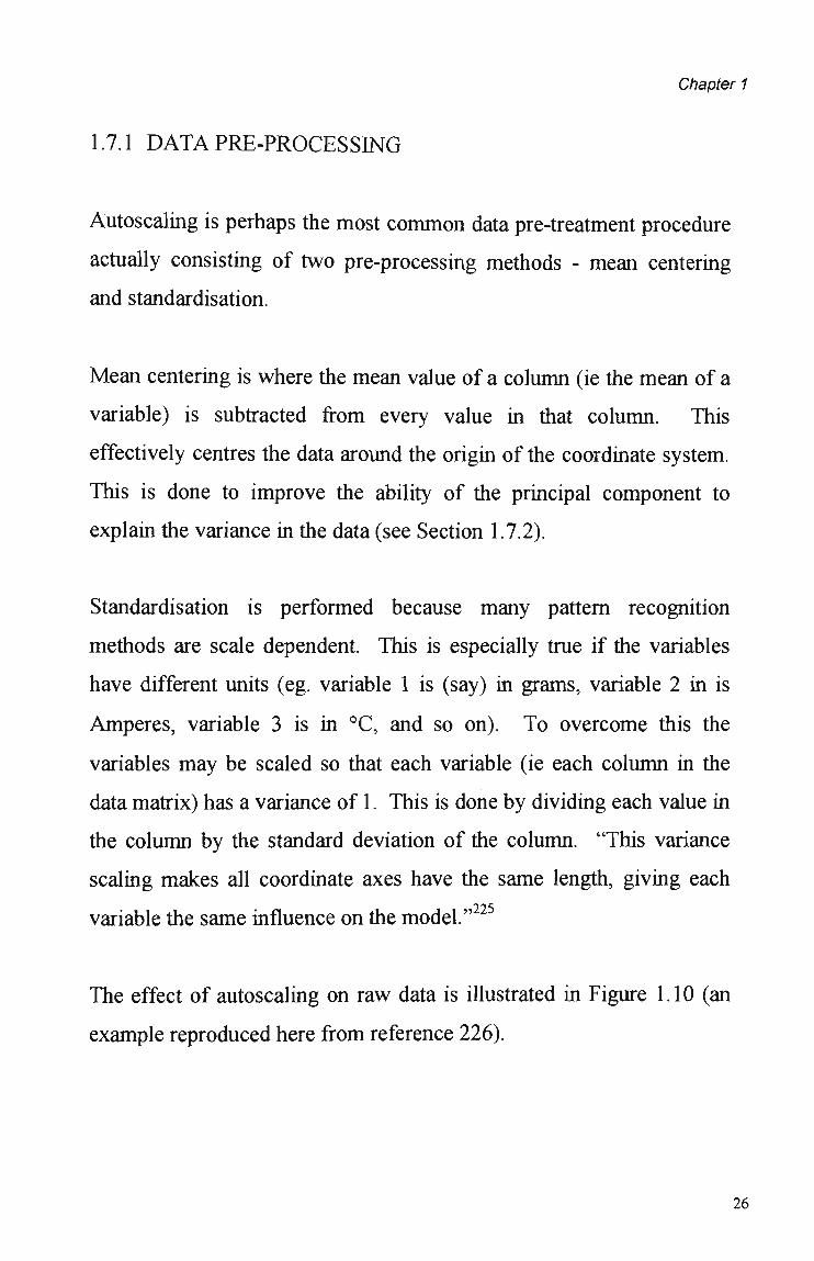
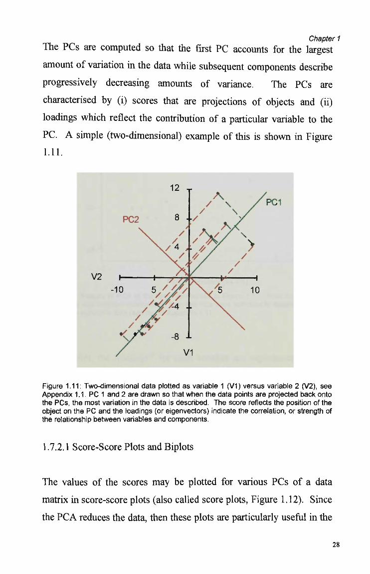
The PCs are computed so that the first P C accounts for the largest

amount of variation in the data while subsequent components describe

progressively decreasing amounts of variance. The PCs are

characterised by (i) scores that are projections of objects and (ii)

loadings which reflect the contribution of a particular variable to the

PC. A simple (two-dimensional) example of this is shown in Figure

1.11.

Figure 1.11: Two-dimensional data plotted as variable 1 (V1) versus variable 2 (V2), see Appendix 1.1. P C 1 and 2 are drawn so that when the data points are projected back onto the PCs, the most variation in the data is described. The score reflects the position of the object on the P C and the loadings (or eigenvectors) indicate the correlation, or strength of the relationship between variables and components.

1.7.2.1 Score-Score Plots and Biplots

The values of the scores may be plotted for various PCs of a data

matrix in score-score plots (also called score plots, Figure 1.12). Since

the PCA reduces the data, then these plots are particularly useful in the

28

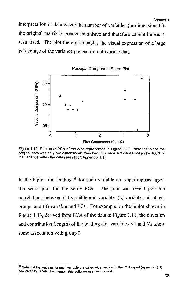
Chapter 1

interpretation of data where the number of variables (or dimensions) in

the original matrix is greater than three and therefore cannot be easily

visualised. The plot therefore enables the visual expression of a large

percentage of the variance present in multivariate data.

Principal Component Score Plot

o*-íO in

c tu c o Q.

£ o O •o

c o ü o CO

05-

00-

05-

• • •

T 1 p -1 0 1

First Component (94.4%)

Figure 1.12: Results of P C A of the data represented in Figure 1.11. Note that since the original data was only two dimensional, then two PCs were sufficient to describe 100% of the variance within the data (see report Appendix 1.1)

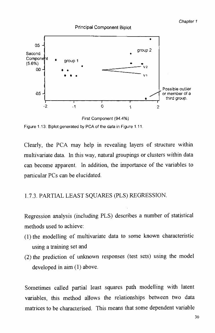
In the biplot, the loadings® for each variable are superimposed upon

the score plot for the same PCs. The plot can reveal possible

correlations between (1) variable and variable, (2) variable and object

groups and (3) variable and PCs. For example, in the biplot shown in

Figure 1.13, derived from PCA of the data in Figure 1.11, the direction

and contribution (length) of the loadings for variables VI and V2 show

some association with group 2.

• Note that the loadings for each variable are called eigenvectors in the PCA report (Appendix 1.1) generated by SCAN, the chemometric software used in this work.

29

Chapter 1

Principal Component Biplot

05 -\

Second Componejit (5.6%)

00 -A

05-Possible outlier or member of a third group.

First Component (94.4%)

Figure 1.13: Biplot generated by PCA of the data in Figure 1.11.

Clearly, the PCA may help in revealing layers of structure within

multivariate data. In this way, natural groupings or clusters within data

can become apparent. In addition, the importance of the variables to

particular PCs can be elucidated.

1.7.3. PARTIAL LEAST SQUARES (PLS) REGRESSION.

Regression analysis (including PLS) describes a number of statistical

methods used to achieve:

(1) the modelling of multivariate data to some known characteristic

using a training set and

(2) the prediction of unknown responses (test sets) using the model

developed in aim (1) above.

Sometimes called partial least squares path modelling with latent

variables, this method allows the relationships between two data

matrices to be characterised. This means that some dependent variable

30

Chapter 1

(eg concentration) can be related to an independem variable data

matrix (eg the responses of a series of sensors) via a mathematical

model.

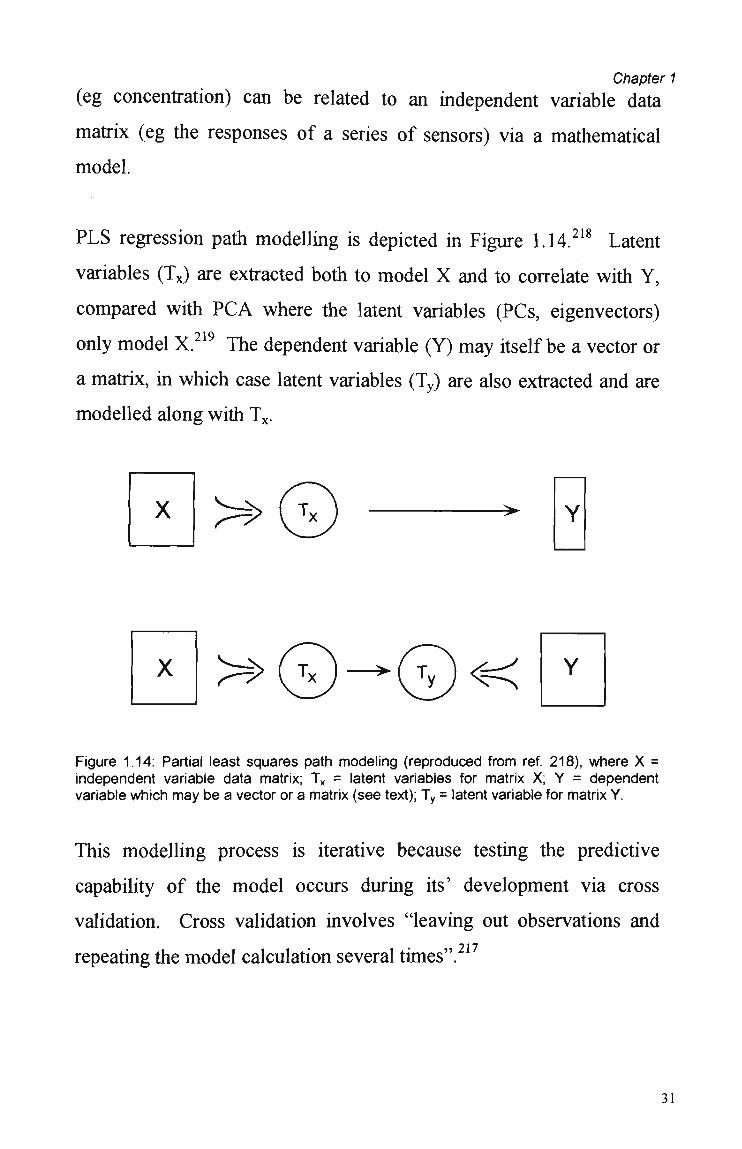
PLS regression path modelling is depicted in Figure 1.14.218 Latent

variables (Tx) are extracted both to model X and to correlate with Y,

compared with P C A where the latent variables (PCs, eigenvectors)

only model X.219 The dependent variable (Y) may itself be a vector or

a matrix, in which case latent variables (Ty) are also extracted and are

modelled along with Tx.

=>

^ ^

Figure 1.14: Partial least squares path modeling (reproduced from ref. 218), where X = independent variable data matrix; Tx = latent variables for matrix X; Y = dependent variable which may be a vector or a matrix (see text); Ty = latent variable for matrix Y.

This modelling process is iterative because testing the predictive

capability of the model occurs during its' development via cross

validation. Cross validation involves "leaving out observations and

repeating the model calculation several times' 217

31

There is NO p. 32 in original document

Chapter 1

aspects were each addressed and integrated into the final synthetic

sensing system.

Iríevitably, this was a multidisciplinary effort, with the various

practical requirements being documented in Chapter 2. These included

production and characterisation of the C E P coated sensor arrays,

chromatographic analysis of anion and cations as well as the hardware

and software specifications of the multichannel potentiostat, data

acquisition and pattern recognition components.

The synthesis strategies and the characterisation of a range of

reproducible conducting electroactive polymer sensors were addressed

in Chapter 3.

The extraction of an amperometric analytical signal from the sensors is

the subject of Chapter 4. The likely effects of the modulation of

various detection parameters on the selectivity of the sensors are

discussed.

Since the aim was to ultimately produce a generic electrochemical

detection system for ion chromatography, then chromatographic

conditions were used throughout this work, (ie the use of columns,

suppressors, certain flow rates and operating pressures, etc). The

selective detection of a range of simple anions and cations after their

separation by ion chromatography is demonstrated in Chapter 5. Also

shown is the effectiveness of changing certain chemical,

electrochemical and kinetic detection parameters. The analytical

performance of the sensors is also discussed here.

Chapter 1

Chapter 6 further examines the chemical and electrochemical

selectivity of the sensors through the chemometric analysis of certain

C V and flow injection analysis (FIA) results. Note that although FIA

procedures were used (in addition to chromatographic ones),

chromatographic conditions (eluent, suppression, operating pressures,

etc) were maintained regardless.

Finally, the application of the sensing system to the determination of

peak purity provided a demonstration of the power of the integrated

sensing system to analyse mixtures. In particular the analysis of

potassium and methylamine mixtures was investigated (Chapter 7).

These cations are known to coelute during H P L C analysis (under

cornmon chromatographic conditions using a Dionex C S 12 column,

etc, Table 2.2). The conventional electroinactive ion detection method

(conductivity) is unable to discriminate between purê and impure

peaks. The determination of peak integrity is therefore a valid

application of the synthetic sensing system developed in this work.

34

Chapter 2

CHAPTER 2

EXPERIMENTAL PROCEDURES.

The experimental methods used in this work are drawn from

electrochemical, analytical, and chemometric disciplines and are grouped

accordingly in this chapter. However one section (Section 2.3) has been

dedicated to the discussion of the multichannel potentiostat, control and

data acquisition systems (designed and constructed by Electrochemical

and Medicai Systems Ltd, UK.), as they are an unique instrumental

component of the final sensing system.

2.1 ELECTROCHEMICAL METHODS

2.1.1 POLYMER SYNTHESIS

Galvanostatic (ie application of a constant current density) deposition

from aqueous monomer/counterion solutions was the method of choice

for polymer synthesis (the optimisation of synthesis conditions is the

subject of Chapter 3).

2.1.1.1 Reagents and Solutions

Pyrrole (Merck) was freshly distilled prior to use and was stored under

Nitrogen at approximately -15 °C. The counterion reagents were used as

received, without further purification. Ali solutions were made up in

deionised (Milli-Q) water and were deoxygenated with Nitrogen for

several minutes before polymerisation.

35

Chapter 2

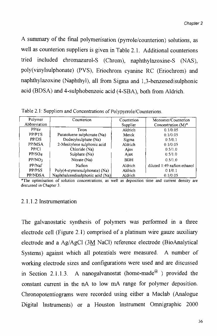
A summary of the final polymerisation (pyrrole/counterion) solutions, as

well as counterion suppliers is given in Table 2.1. Additional counterions

tried included chromazurol-S (Chrom), naphthylazoxine-S (NAS),

poly(vinylsulphonate) (PVS), Eriochrom cyanine R C (Eriochrom) and

naphthylazoxine (Naphthyl), ali from Sigma and 1,3-benzenedisulphonic

acid (BDSA) and 4-sulphobenzoic acid (4-SBA), both from Aldrich.

Table 2.1: Suppliers and Concentrations of Polypyrrole/Counterions.

Polymer Abbreviation

PP/tir PP/PTS PP/DS PP/MSA PP/Cl

PP/SO4

PP/NO3

PP/Naf PP/PSS

PP/NDSA

Counterion

Tiron Paratoluene sulphonate (Na)

Dodecylsulphate (Na) 2-Mesitylene sulphonic acid

Chloride (Na) Sulphate (Na)

Nitrate (Na)

Nafion Poly(4-styrenesulphonate) (Na)

Naphthalenedisulphonic acid (Na)

Counterion Supplier

Aldrich Merck Sigma Aldrich Ajax Ajax

BDH Aldrich Aldrich Aldrich

Monomer/Counterion Concentration (M)*

0.1/0.05 0.1/0.05 0.5/0.1 0.1/0.05 0.5/1.0 0.5/1.0

0.5/1.0

diluted 1:49 nafion: ethanol 0.1/0.1 0.1/0.05

*The optimisation of solution concentrations, as well as deposition time and current density are discussed in Chapter 3.

2.1.1.2 Instrumentation

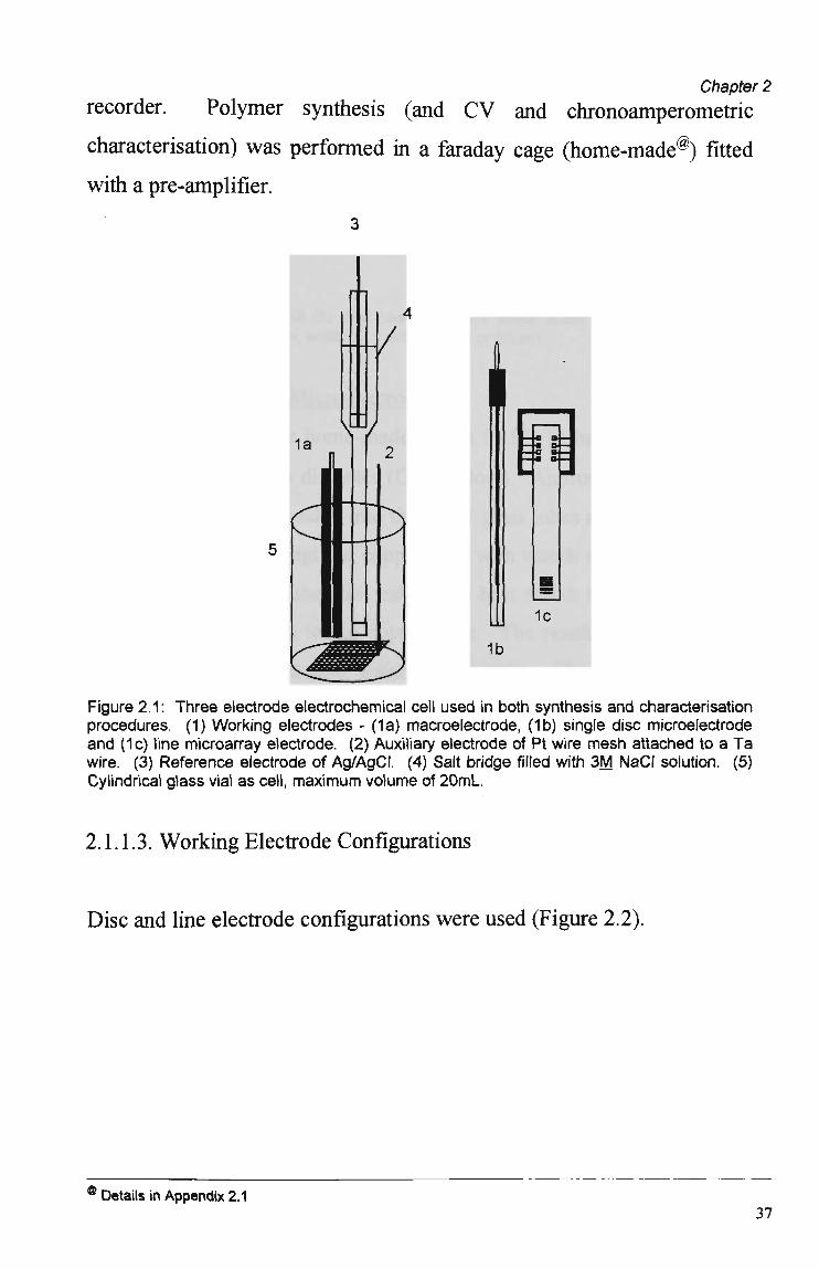
The galvanostatic synthesis of polymers was performed in a three

electrode cell (Figure 2.1) comprised of a platinum wire gauze auxiliary

electrode and a Ag/AgCI (3M NaCl) reference electrode (BioAnalytical

Systems) against which ali potentials were measured. A number of

working electrode sizes and configurations were used and are discussed

in Section 2.1.1.3. A nanogalvanostat (home-made® ) provided the

constant current in the n A to low m A range for polymer deposition.

Chronopotentiograms were recorded using either a Maclab (Analogue

Digital Instruments) or a Houston Instrument Omnigraphic 2000

36

Chapter 2

recorder. Polymer synthesis (and C V and chronoamperometric

characterisation) was performed in a faraday cage (home-made@) fitted

with a pre-amplifier.

3

1a

II

r jSSt

4

V

7 2

WJ Figure 2.1: Three electrode electrochemical cell used in both synthesis and characterisation procedures. (1) Working electrodes - (1a) macroelectrode, (1b) single disc microelectrode and (1c) line microarray electrode. (2) Auxiliary electrode of Pt wire mesh attached to a Ta wire. (3) Reference electrode of Ag/AgCI. (4) Salt bridge filled with 3 M NaCl solution. (5) Cylindrical glass viai as cell, maximum volume of 2 0 m L

2.1.1.3. Working Electrode Confígurations

Disc and line electrode confígurations were used (Figure 2.2).

Details in Appendix 2.1 37

Chapter 2

A B Figure 2.2: Configuration of (A) disc (diameter (a) = either 50p.m or 10um) and (B) line electrodes (length (c) = 1mm, width (b) = either 10um or 50um),

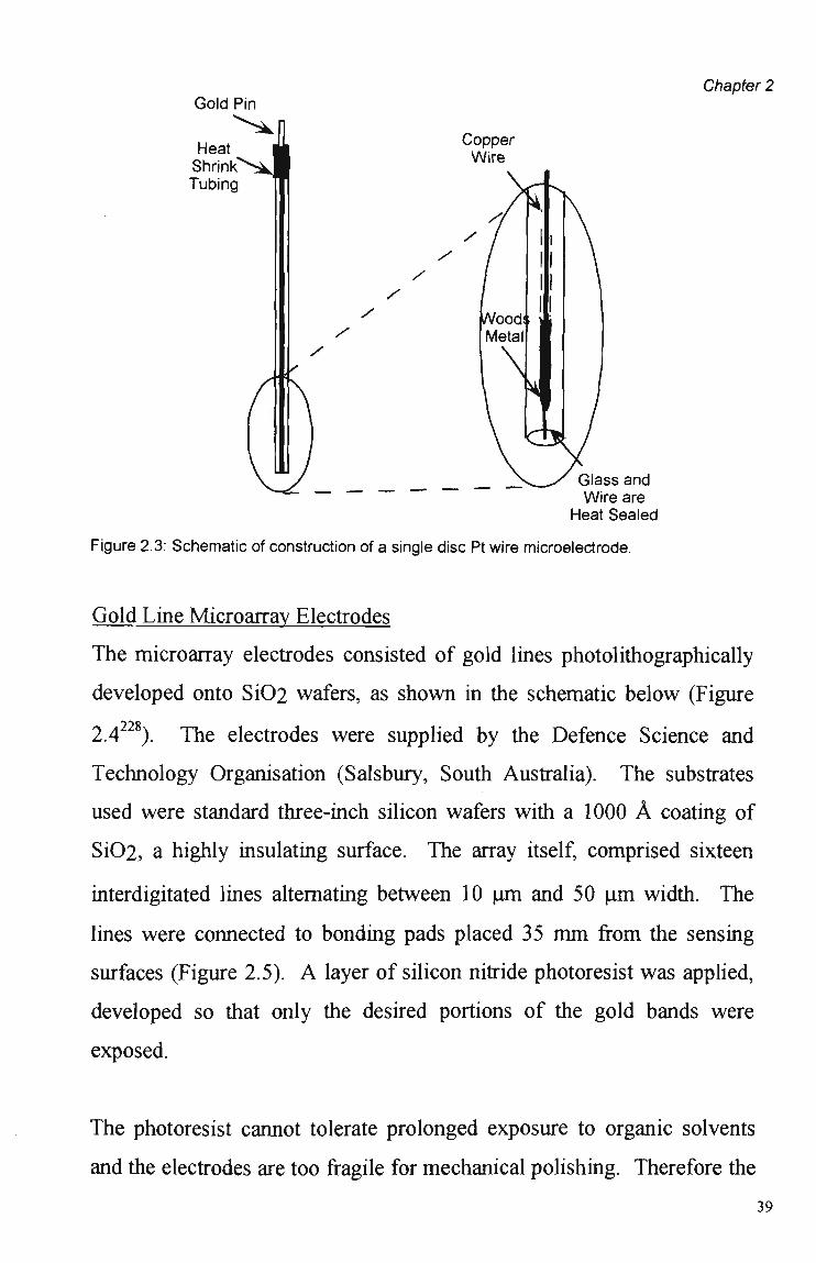
Single Disc Platinum Microelectrodes

These electrodes were home-made@ from 99.9% Pt hard temper wire of

either 50um or lOum diameter (Goodfellow). Approximately 1.5cm of

the Pt wire was heat-sealed into the tip of glass tubes and the end within

the tube joined to a length of copper wire with woods metal (Figure 2.3).

The open end of the tube was sealed with heat shrink tubing once a gold

pin had been attached to the copper wire. The resulting electrode was

reasonably robust and also water and airtight. The Pt/glass end was

ground down by successively finer grades of emery paper (lubricated

with distilled water). Finally, the electrodes were polished with a 0.05

u m alumina/water slurry (Leco) on a polishing pad (Leco).

Details in Appendix 2.1 38

Gold Pin

Heat Shrink^^ Tubing 3

Copper Wire

/

/

/ /

/

Chapter 2

Glass and Wire are

Heat Sealed

Figure 2.3: Schematic of construction of a single disc Pt wire microelectrode.

Gold Line Microarray Electrodes

The microarray electrodes consisted of gold lines photolithographically

developed onto Si02 wafers, as shown in the schematic below (Figure

2.4228). The electrodes were supplied by the Defence Science and

Technology Organisation (Salsbury, South Austrália). The substrates

used were standard three-inch silicon wafers with a 1000 Â coating of

Si02, a highly insulating surface. The array itself, comprised sixteen

interdigitated lines alternating between 10 u m and 50 u m width. The

lines were connected to bonding pads placed 35 m m from the sensing

surfaces (Figure 2.5). A layer of silicon nitride photoresist was applied,

developed so that only the desired portions of the gold bands were

exposed.

The photoresist cannot tolerate prolonged exposure to organic solvents

and the electrodes are too fragile for mechanical polishing. Therefore the

39

Chapter 2

cleaning of dust and residual solvent from the photolithographic process

was performed by gentle swabbing with a soft cotton bud soaked with

dilute dextran (approximately 4:1 water:dextran), rinsing with deionised

water and finally, drying with a gentle N 2 gas stream.

1

a

. ^ M T

u u v u u t • r

••• "'• ^ M K^I im^ ll»d

g Figure 2.4: Schematic of microlíthographic procedure: (a) Photoresist (1um) spun onto Si02 wafer (b) Photoresist exposed through mask 1; (c) Photoresist developed for metal patterning; (d) Gold layer vapour-deposited; (e) Lift off unwanted metal with acetone; (f) Second layer of photoresist spun onto wafer; (g) Photoresist exposeçyhrough mask 2; (h) Photoresist developed leaving gold surface exposed in desired pattern.

40

Chapter 2

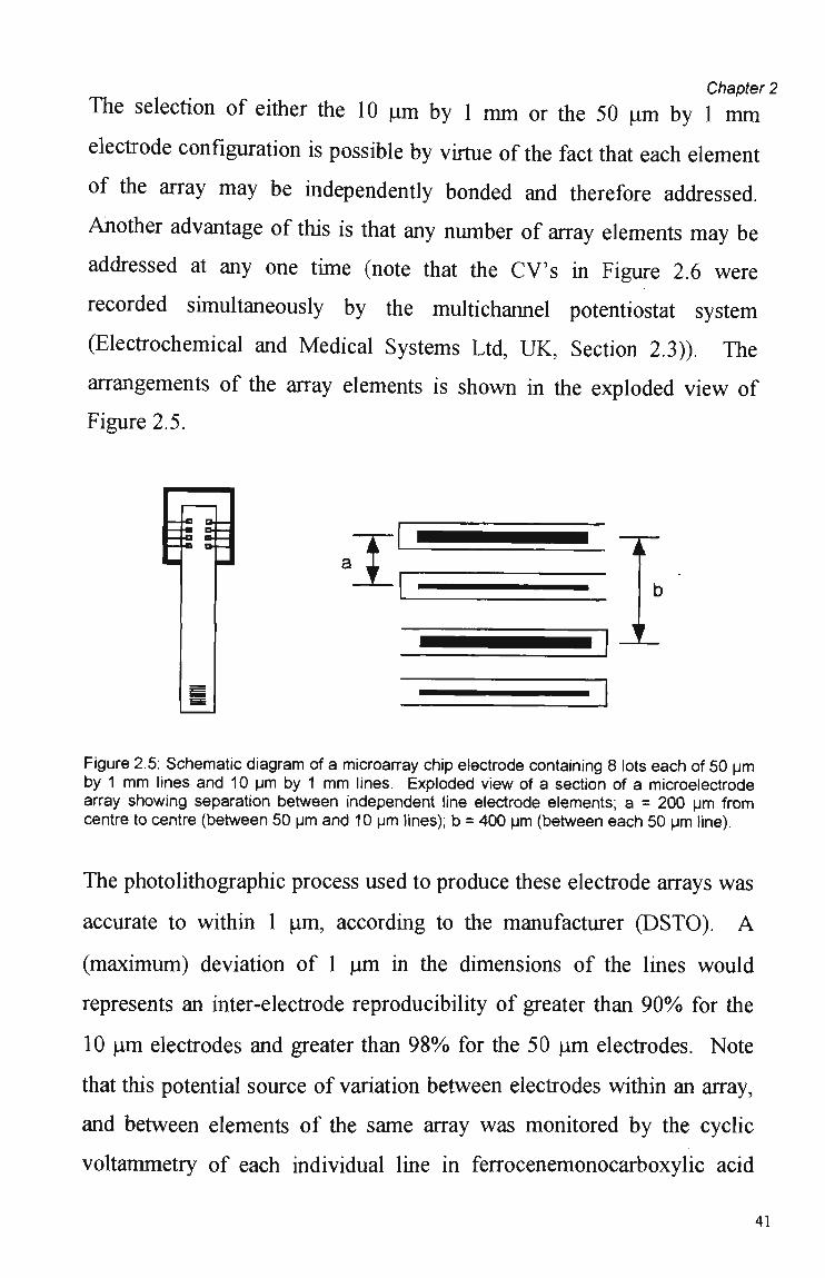
The selection of either the 10 u m by 1 m m or the 50 u m by 1 m m

electrode configuration is possible by virtue of the fact that each element

of the array may be independently bonded and therefore addressed.

Another advantage of this is that any number of array elements may be

addressed at any one time (note that the C V s in Figure 2.6 were

recorded simultaneously by the multichannel potentiostat system

(Electrochemical and Medicai Systems Ltd, UK, Section 2.3)). The

arrangements of the array elements is shown in the exploded view of

Figure 2.5.

Figure 2.5: Schematic diagram of a microarray chip electrode containing 8 lots each of 50 pm by 1 m m lines and 10 um by 1 m m lines. Exploded view of a section of a microelectrode array showing separation between independent line electrode elements; a = 200 pm from centre to centre (between 50 pm and 10 pm lines); b = 400 pm (between each 50 pm line).

The photolithographic process used to produce these electrode arrays was

accurate to within 1 um, according to the manufacturer (DSTO). A

(maximum) deviation of 1 u m in the dimensions of the lines would

represents an inter-electrode reproducibility of greater than 9 0 % for the

10 (am electrodes and greater than 9 8 % for the 50 u m electrodes. Note

that this potential source of variation between electrodes within an array,

and between elements of the same array was monitored by the cyclic

voltammetry of each individual line in ferrocenemonocarboxylic acid

41

Chapter 2

( F M C A ) as described below. This provided a constant check of every

electrode used in this work and showed that the bare electrode could not

account for ali of the variability seen for the deposition of various

polymers investigated (discussed further in Chapter 3, Section 3.3.1.3).

As mentioned above, the electrochemical performance of each array was

checked prior to polymer deposition by cyclic voltammetry (Section

2.1.2.1) in a 1 m M solution of ferrocenemonocarboxylic acid (FMCA,

Aldrich) in a 0.5 M N a H 2 P 0 4 ( B D H ) supporting electrolyte, p H adjusted

to neutral with N a O H .

The CVs revealed that the line confígurations do exhibit a degree of

microelectrode behaviour (as discussed in Section 1.4.1) though the one

"macro" dimension of the line (Figure 2.6) obviously should not be

discounted. Indeed it is likely that this "macro" dimension is largely

responsible for the relative ease and reproducibility of polymer

deposition encountered with the 50 jim line electrodes (Section 3.3).

42

20nA

I I 1 1 1 1 •0.1 0.0 0.1 0.2 0.3 0.4

E(V) vs Ag/AgCI

Chapter 2

•0.1 0.0 0.1 0.2 0.3 0.4

E(V) vs Ag/AgCI

A B Figure 2.6: CVs of electrodes of (A)10 pm by 1 mm dimensions and (B) 50 pm by 1 mm dimensions run in 1 m M ferrocenemonocarboxylic acid solution (FMCA) with phosphate buffer (pH = 7) supporting electrolyte; scan rate = 25 mV/s .

Further, the line elements are spaced suffíciently apart so that the

diffusion layer of each element does not influence those of the

neighbouring electrodes. This was apparent when the CVs of one

element were recorded first with and then without the adjacent lines

being connected (Figure 2.7).

43

Chapter 2

•0.1 0.0 0.1 0.2 0.3 0.4

E(V) vs Ag/AgCI E(V) vs Ag/AgCI

Figure 2.7: CVs of electrodes of 50 um by 1 m m line dimensions run in 1 m M F M C A solution with phosphate buffer (pH = 7) supporting electrolyte; scan rate = 25 mVs"1 (A) without neighbouring electrodes connected (B) with neighbouring electrodes connected.

A second array configuration was also used, which comprised 10 lines of

20 u m by 1 m m dimensions. The lines of this array were not individually

addressable (ie ali were connected to each other). A representation of

this electrode configuration is shown in Figure 2.8.

Figure 2.8: A gold microarray electrode, 10 lines of 20 pm by 1 m m dimensions.

2.1.2 POLYMER CHARACTERISATION

Cyclic Voltammetry, Chronoamperometry

The electrochemical behaviour of the polymers produced was assessed by

cyclic voltammetry (CV) in various supporting electrolytes. In this way,

polymer electroactivity, reproducibility and stability were examined.

CVs were also considered for preliminary investigations into polymer

44

Chapter 2

selectivity (the subject of Chapter 5), since regions of anion and cation

movement m a y be discerned with this technique. Another

characterisation techniques utilised in this work was chronoamperometry

(the study of the polymer's response to pulsed potential stimuli,

introduced in Section 1.5.2).

Scanning Electron Microscopy.

Scanning electron microscopy (SEM) is useful in probing the

morphology and physical uniformity of polymer surfaces. Unfortunately,

because the samples (and electrodes) are destroyed during S E M analysis,

only polymers grown on the disposable array electrodes could be

characterised with this technique.

2.1.2.1 Reagents and Solutions

Various supporting electrolytes were used in both CV and

chronoamperometry including Na2S04, NaCl, K and methylamine (MA,

from Aldrich), of various concentrations, specified where appropriate in

the text. Ali were made up in deionised water, and were deoxygenated

with N 2 gas prior to either C V or chronoamperometric studies.

2.1.2.2 Instrumentation

The CV and chronoamperograms were performed in the same three

electrode cell as used in polymer deposition (Figure 2.1) and were

recorded using either an Electrolab ( A D Instruments) or the multichannel

data acquisition system (Electrochemical and Medicai Systems Ltd, U K ,

see Section 2.3).

45

Chapter 2

S E M images were obtained on a Steroscan 440 (Cambridge).

2.2 ANALYTICAL METHODS

2.2.1 ION CHROMATOGRAPHY/FLOW INJECTION ANALYSIS

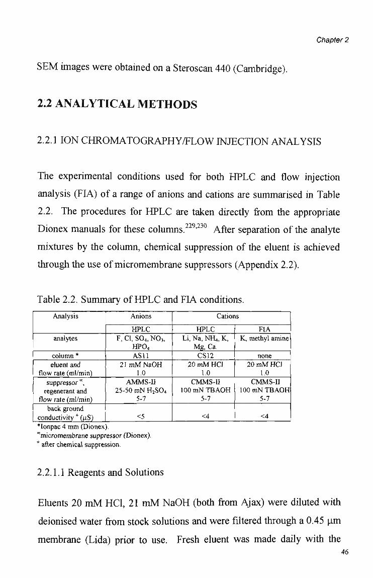
The experimental conditions used for both HPLC and flow injection

analysis (FIA) of a range of anions and cations are summarised in Table

2.2. The procedures for H P L C are taken directly from the appropriate

Dionex manuais for these columns.229'230 After separation of the analyte

mixtures by the column, chemical suppression of the eluent is achieved

through the use of micromembrane suppressors (Appendix 2.2).

Table 2.2. Summary of H P L C and FIA conditions.

Analysis

analytes

column * eluent and

flow rate (ml/min) suppressor *, regenerant and

flow rate (ml/min) back ground

conductivity + (uS)

Anions

HPLC F,C1,S04,N03,

HP04

AS11 21 mMNaOH

1.0 AMMS-II

25-50 mNH2S04

5-7

<5

Cations

HPLC Li, Na, NH4, K,

Mg, Ca. CS 12

20mMHCl 1.0

CMMS-II 100 mN TBAOH

5-7

<4

FIA K, methyl amine

none 20mMHCl

1.0 CMMS-II

100 mN TBAOH 5-7

<4 *Ionpac 4 m m (Dionex). "micromembrane suppressor (Dionex). + after chemical suppression.

2.2.1.1 Reagents and Solutions

Eluents 20 mM HCI, 21 mM NaOH (both from Ajax) were diluted with

deionised water from stock solutions and were filtered through a 0.45 jam

membrane (Lida) prior to use. Fresh eluent was made daily with the 46

Chapter 2

N a O H kept under a Nitrogen environment to prevent the formation of

carbonates. Regenerant solutions were 50 m N H2SO4 (Ajax) and 100

m N TBAOH.30H2O (Fluka).

Anion stock solution mixtures (1000 ppm) were made up of NaCl,

Na2S04 (Ajax), NaN03, NaF and Na2HP04 (BDH) in Müli-Q water (or

were obtained from Dionex). Standards for H P L C were diluted from this

stock using the fresh N a O H eluent. Cation standards were similarly

prepared from 1000 ppm stock solutions mixtures of KCI, MgCl2.6H20

(BDH), NH4CI, LiCl, CaCl2.2H20 (Ajax), diluted with fresh HCI eluent.

Table 2.3 Retention times for cation and anion chromatography*.

Analytes

Fluoride Chloride Sulphate Nitrate

Phosphate Lithium Sodium

Ammonium Potassium Magnesium Calcium

Retention Time (seconds)

77 96 133 148 305 157 186 217 278 336 418

* Using conditions stated in Table 2.2.

Potassium and methylamine hydrochloride (MA, from Aldrich) cation

standards for FIA were similarly made up in the HCI eluent which was

then suppressed (as for cation HPLC). This was to ensure that the

chemical nature of the eluent for both H P L C and FIA were the same and

as such could not cause any differences in polymer selectivity behaviour.

47

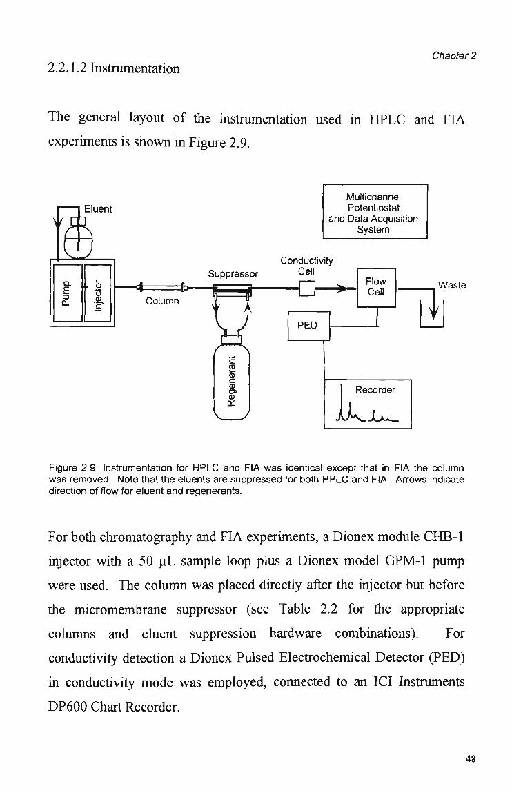
2.2.1.2 Instrumentation Chapter 2

The general layout of the instrumentation used in H P L C and FIA

experiments is shown in Figure 2.9.

Y k

Eluent

)

CL

E o_

fc-

• £ o (D

Multichannel Potentiostat

and Data Acquisition System

Waste

Figure 2.9: Instrumentation for H P L C and FIA was identical except that in FIA the column was removed. Note that the eluents are suppressed for both H P L C and FIA. Arrows indicate direction of flow for eluent and regenerants.

For both chromatography and FIA experiments, a Dionex module CHB-1

injector with a 50 uL sample loop plus a Dionex model GPM-1 pump

were used. The column was placed directly after the injector but before

the micromembrane suppressor (see Table 2.2 for the appropriate

columns and eluent suppression hardware combinations). For

conductivity detection a Dionex Pulsed Electrochemical Detector (PED)

in conductivity mode was employed, connected to an ICI Instruments

DP600 Chart Recorder.

48

Chapter 2

The electrochemical cell was a BAS thin layer flow cell in which the

microelectrode arrays were sandwiched between the upper and lower

halves of the cell (Figure 2.10). The stainless steel upper half of the cell

served as the auxiliary electrode and a Ag/AgCI reference was placed

immediately downstream of the cell.

Inlet

\ *

I / Reference Electrode

Stainless Steel Upper Block (Auxiliary)

->- Waste Outlet

Direction Of Flow

Gasket

• H M Array Electrode

(Working)

Figure 2.10: BAS flow cell with array electrode

The electrode was positioned in the cell so that the array elements were

centred in the flow path (Figure 2.11).

Direction O f Flow > •

Connections to Potentiostat. Figure 2.11: Plan view of array working electrode and gasket showing position of electrode array.

49

Chapter 2

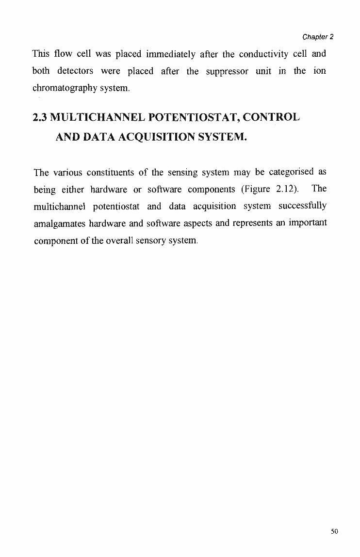
This flow cell was placed immediately after the conductivity cell and

both detectors were placed after the suppressor unit in the ion

chromatography system.

2.3 MULTICHANNEL POTENTIOSTAT, CONTROL

AND DATA ACQUISITION SYSTEM.

The various constituents of the sensing system may be categorised as

being either hardware or software components (Figure 2.12). The

multichannel potentiostat and data acquisition system successfully

amalgamates hardware and software aspects and represents an important

component of the overall sensory system.

50

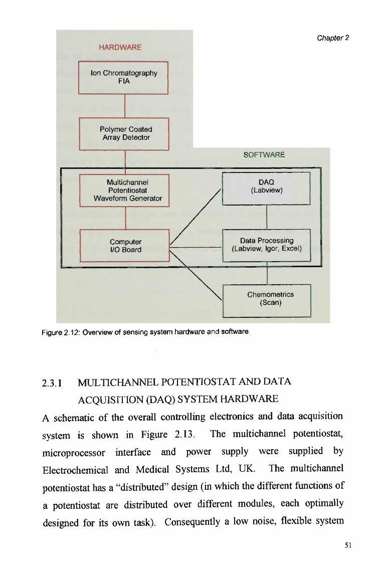
Chapter 2 HARDWARE

Ion Chromatography FIA

Polymer Coated Array Detector

S O F T W A R E

Multichannel Potentiostat

Waveform Generator

Computer l/O Board

/

/

/

\

\

^

DAQ (Labview)

Data Processing (Labview, Igor, Excel)

Chemometrics (Scan)

Figure 2.12: Overview of sensing system hardware and software.

2.3.1 MULTICHANNEL POTENTIOSTAT AND DATA

ACQUISITION (DAQ) S Y S T E M H A R D W A R E

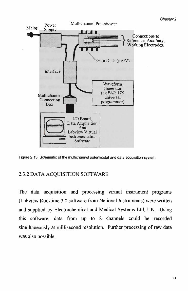
A schematic of the overall controlling electronics and data acquisition

system is shown in Figure 2.13. The multichannel potentiostat,

microprocessor interface and power supply were supplied by

Electrochemical and Medicai Systems Ltd, UK. The multichannel

potentiostat has a "distributed" design (in which the different functions of

a potentiostat are distributed over different modules, each optimally

designed for its own task). Consequenüy a low noise, flexible system

Chapter 2

capable of controlling the potential and measuring the currents of up to

eight electrodes simultaneously results. A single reference electrode was

required. Externai potential sources to generate the desired potential

waveforms at each of the working electrodes may be used, and was

supplied by either a P A R 175 universal programmer or a waveform

generator (home-made@). The later waveform generator could be

programmed for symmetric and asymmetric pulsed and scanned potential

waveforms.

The data acquisition system was comprised of a general purpose input-

output board (NB-MIO-16X), and a multichannel connection box, both

supplied by National Instruments. The I/O board was placed inside a

Macintosh Quadra 650.

Details in Appendix 2.1 52

Mains Power Supply

Multichannel Potentiostat

• • • •

Chapter 2

} C o n n e c t i o n s to Reference, Auxiliary, Working Electrodes.

Gain Dials (uA/V)

Interface

Multichannel Connection

Box

Waveform Generator

(eg P A R I 75 universal

programmer)

I/O Board, Data Acquisition

And Labview Virtual Instrumentation

Software

Figure 2.13: Schematic of the multichannel potentiostat and data acquisition system.

2.3.2 D A T A ACQUISITION S O F T W A R E

The data acquisition and processing virtual instrument programs

(Labview Run-time 3.0 software from National Instruments) were written

and supplied by Electrochemical and Medicai Systems Ltd, UK. Using

this software, data from up to 8 channels could be recorded

simultaneously at millisecond resolution. Further processing of raw data

was also possible.

53

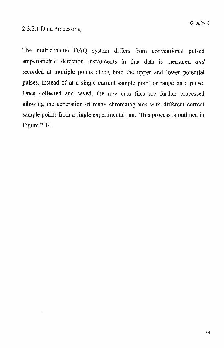
Chapter 2

2.3.2.1 Data Processing

The multichannel DAQ system differs from conventional pulsed

amperometric detection instruments in that data is measured and

recorded at multiple points along both the upper and lower potential

pulses, instead of at a single current sample point or range on a pulse.

Once collected and saved, the raw data files are further processed

allowing the generation of many chromatograms with different current

sample points from a single experimental run. This process is outlined in

Figure 2.14.

54

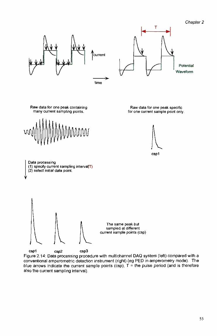
Chapter 2

r burrent Potential

Waveform

time

R a w data for one peak containing many current sampling points.

R a w data for one peak specific for one current sample point only.

cspl

Data processing (1) specify current sampling intervari) (2) seiect initial data point.

The same peak but sampled at different

current sample points (csp)

cspl Csp2 csp3

Figure 2.14: Data processing procedure with multichannel D A Q system (left) compared with a conventional amperometric detection instrument (right) (eg P E D in amperometry mode). The blue arrows indicate the current sample points (csp), T = the pulse period (and is therefore also the current sampling interval).

55

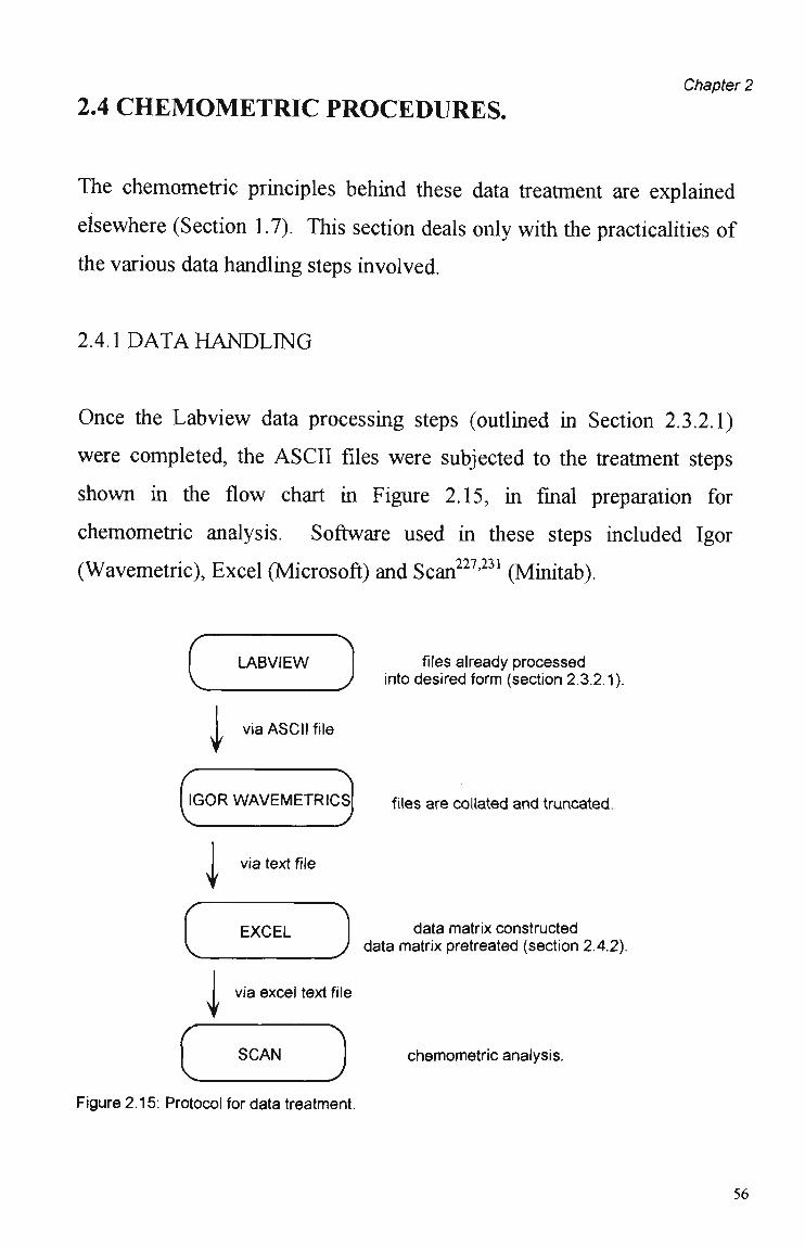
2.4 CHEMOMETRIC PROCEDURES. Chapter 2

The chemometric principies behind these data treatment are explained

elsewhere (Section 1.7). This section deals only with the practicalities of

the various data handling steps involved.

2.4.1 DATA HANDLING

Once the Labview data processing steps (outlined in Section 2.3.2.1)

were completed, the ASCII files were subjected to the treatment steps

shown in the flow chart in Figure 2.15, in final preparation for

chemometric analysis. Software used in these steps included Igor

(Wavemetric), Excel (Microsoft) and Scan227'231 (Minitab).

LABVIEW

i via ASCII file

IGOR W A V E M E T R I C S

files already processed into desired form (section 2.3.2.1).

fites are collated and truncated.

via text file

E X C E L data matrix constructed data matrix pretreated (section 2.4.2).

i via excel text file

S C A N chemometric analysis.

Figure 2.15: Protocol for data treatment.

56

Chapter 3

CHAPTER 3

SYNTHESIS AND CHARACTERISATION OF

POLYMER COATED ELECTRODES

3.1. INTRODUCTION

Sensor selectivity and reproducibility are two indispensable criteria

which governed the development and realisation of the CEP-coated array.

The selectivity aspect was (at least in part) addressed by the synthesis of

polymers with different chemical compositions. The electrochemical

synthesis of various polypyrroles is the subject of this chapter.

The best method of CEP deposition upon microelectrodes is the

electrochemical synthesis route. Electrochemical coating of one bare

electrode at a time via serial immersion of the array and polymerisation in

the various monomer/counterion solutions, is a relatively simple, fast and

reproducible procedure. Galvanostatic deposition was the synthesis

method of choice for this work (Section 2.1.1) as it allowed greater

control over the rate of monomer oxidation, this (In the alternative

potentiostatic method, the current will fluctuate to ensure a constant

potential is maintained, which is not always reproducible.)

Polymer reproducibility was assessed by cyclic voltammetry (CV) and

scanning electron microscopy ( S E M ) and was useful in probing the

morphology and physical uniformity of polymer surfaces. Cyclic

voltammetry can also be a valuable technique for preliminary

investigations into polymer selectivity, however this aspect is dealt with

Chapter 3

in some detail in Chapter 5. Chronoamperometry was also employed, but

the utilisation of this technique is more pertinent to discussions on signal

generation and is documented in Chapter 4.

3.2. EXPERIMENTAL

Electrochemical polymer deposition, characterisation procedures and

instrumentation were discussed previously (Sections 2.1.1 and 2.1.2).

As the arrays were single use only, preliminary polymer synthesis and

characterisation work was performed on 10 \xm and 50 u m diameter Pt

disc electrodes. This reduced the time and costs involved in optimising

the polymer growth conditions. Once reproducible synthesis conditions

had been identifíed, deposition and characterisation was performed on

array electrodes. Electrode confígurations are as described in Section

2.1.1.3.

3.3. RESULTS AND DISCUSSION

3.3.1 POLYMER DEPOSITION

Polymerisation was performed in aqueous media for two important

reasons. Firstly, the array electrodes were constructed from materiais

which cannot tolerate exposure to organic solvents (Section 2.1.1.3.).

Secondly, the electrodes were ultimately required to operate in an

aqueous environment, as detectors of electroinactive anions and cations.

58

Chapter 3

A n important practical limitation was that the growth potential reached

during deposition could not exceed 1.0 V to 1.1 V. This was so that the

array was not damaged by 0 2 bubbles formed when water is oxidised at

the higher potentials (Equation 3.1). These 0 2 bubbles act to

mechanically lift the insulating layer form the electrode edges, changing

the dimensions of the electrode, as well as compromising the mechanical

stability of the electrode.

2H20 *» 4e' + 4H+ + 02 E0 = 1.229V (3.1)

Attempts to grow a number of polymers with different chemical

compositions on 10 u m and 50 u m Pt disc microelectrodes, revealed that

polymer synthesis is dependent on several parameters, including:

(i) the nature of the monomer and/or counterion

(2) the concentration of monomer and/or counterion

(3) the current density

(4) the shape and size of the electrode.

3.3.1.1. The Nature of the Monomer and Counterion

Of the many different monomer (Appendix 3.1) and counterion

(Appendix 3.2) combinations tried, ít was obvious that some were more

difficult to deposit reproducibly onto microelectrodes than others. This

was despite a range of monomer/counterion concentrations and current

densities being investigated in each case. The most successful deposition

occurred with the pyrrole monomer in combination with a range of

counterions. "Success" was established via C V in either 10'4M NaCl or

59

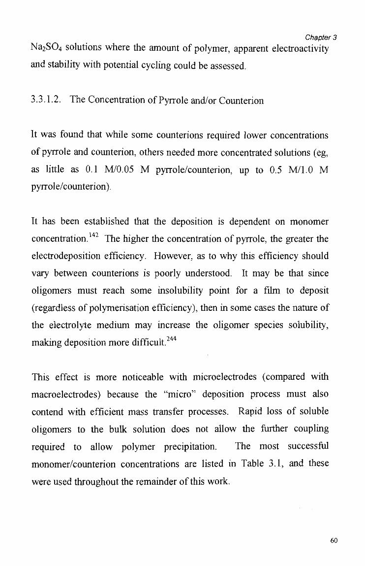
Chapter 3

N a 2 S 0 4 solutions where the amount of polymer, apparent electroactivity

and stability with potential cycling could be assessed.

3.3.1.2. The Concentration of Pyrrole and/or Counterion

It was found that while some counterions required lower concentrations

of pyrrole and counterion, others needed more concentrated solutions (eg,

as little as 0.1 M/0.05 M pyrrole/counterion, up to 0.5 M/1.0 M

pyrrole/counterion).

It has been established that the deposition is dependent on monomer

concentration.142 The higher the concentration of pyrrole, the greater the

electrodeposition efficiency. However, as to w h y this efficiency should

vary between counterions is poorly understood. It m a y be that since

oligomers must reach some insolubility point for a film to deposit

(regardless of polymerisation efficiency), then in some cases the nature of

the electrolyte médium may increase the oligomer species solubility,

making deposition more difficult.24

This effect is more noticeable with microelectrodes (compared with

macroelectrodes) because the "micro" deposition process must also

contend with efficient mass transfer processes. Rapid loss of soluble

oligomers to the bulk solution does not allow the further coupling

required to allow polymer precipitation. The most successful

monomer/counterion concentrations are listed in Table 3.1, and these

were used throughout the remainder of this work.

60

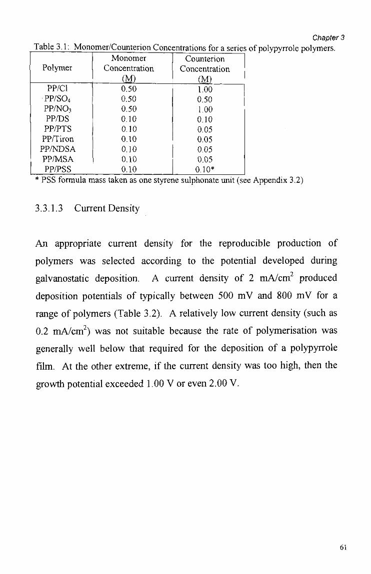
Chapter 3 Table 3.1: Monomer/Counterion Concentrations for a series of polypyrrole polymers.

Polymer

PP/Cl PP/S04

PP/NO3 PP/DS PP/PTS PP/Tiron PP/NDSA PP/MSA PP/PSS

Monomer Concentration

(M) 0.50 0.50 0.50 0.10 0.10 0.10 0.10 0.10 0.10

Counterion Concentration

(M) 1.00 0.50 1.00 0.10 0.05 0.05 0.05 0.05 0.10*

* PSS formula mass taken as one styrene sulphonate unit (see Appendix 3.2)

3.3.1.3 Current Density

A n appropriate current density for the reproducible production of

polymers was selected according to the potential developed during

galvanostatic deposition. A current density of 2 m A / c m produced

deposition potentials of typically between 500 m V and 800 m V for a

range of polymers (Table 3.2). A relatively low current density (such as

0.2 mA/cm 2) was not suitable because the rate of polymerisation was

generally well below that required for the deposition of a polypyrrole

film. At the other extreme, if the current density was too high, then the

growth potential exceeded 1.00 V or even 2.00 V.

61

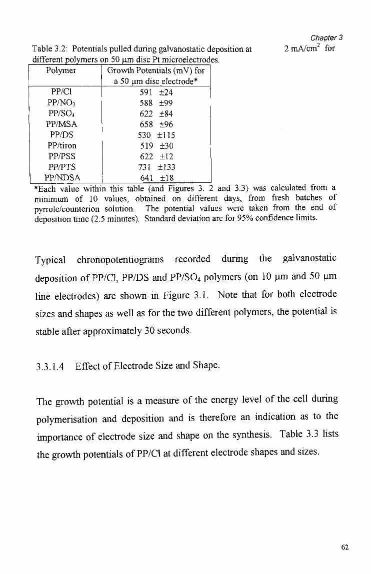
Table 3.2: Potentials pulled during galvanostatic deposition at different polymers on 50 im disc Pt microelectrodes.

Chapter 3 2 mA/cm2 for

Polymer \

PP/Cl PP/N03

PP/SO4 PP/MSA PP/DS PP/tiron PP/PSS PP/PTS PP/NDSA

Growth Potentials (mV) for a 50 p m disc electrode*

591 ±24 588 ±99 622 ±84 658 ±96 530 ±115 519 ±30 622 ±12 731 ±133 641 ±18

*Each value within this table (and Figures 3. 2 and 3.3) was calculated from a minimum of 10 values, obtained on different days, from fresh batches of pyrrole/counterion solution. The potential values were taken from the end of deposition time (2.5 minutes). Standard deviation are for 9 5 % confídence limits.

Typical chronopotentiograms recorded during the galvanostatic

deposition of PP/Cl, PP/DS and PP/SO4 polymers (on 10 u m and 50 u m

line electrodes) are shown in Figure 3.1. Note that for both electrode

sizes and shapes as well as for the two different polymers, the potential is

stable after approximately 30 seconds.

3.3.1.4 Effect of Electrode Size and Shape.

The growth potential is a measure of the energy levei of the cell during

polymerisation and deposition and is therefore an indication as to the

importance of electrode size and shape on the synthesis. Table 3.3 lists

the growth potentials of PP/Cl at different electrode shapes and sizes.

62

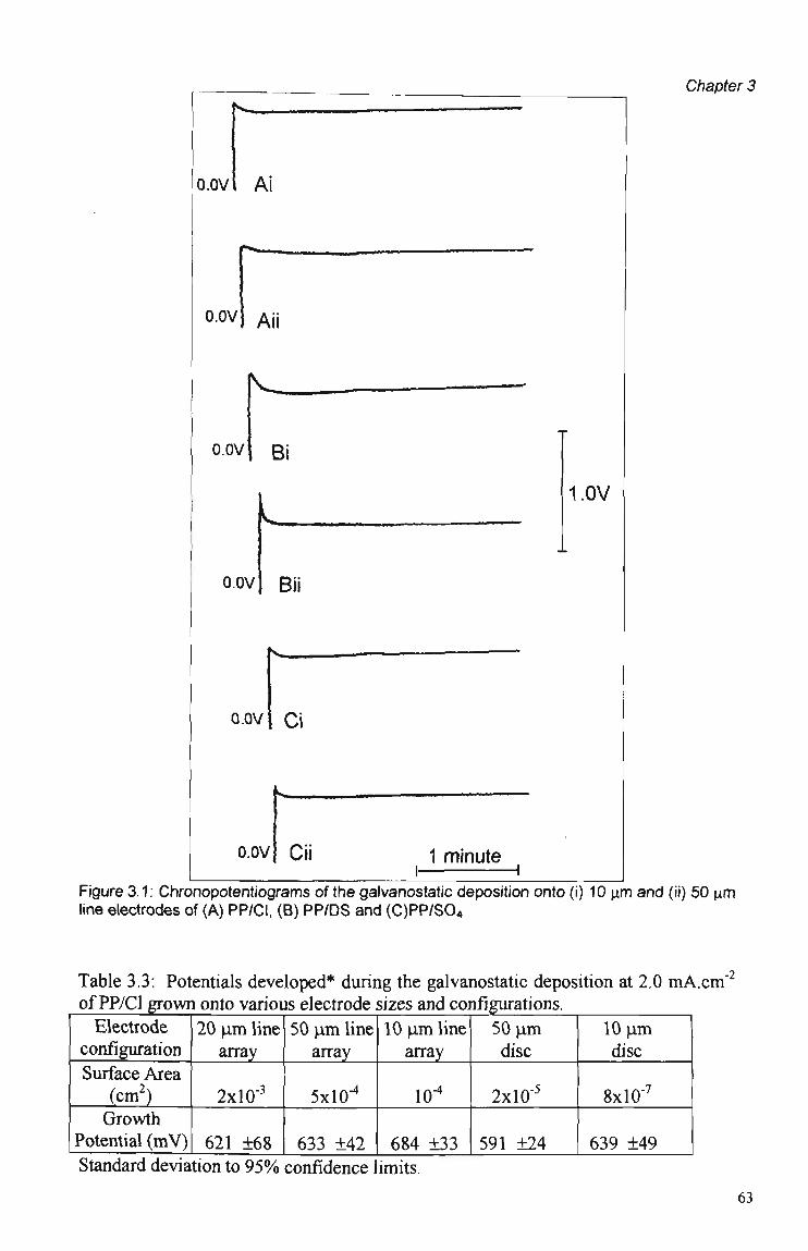
fs^.

o.ov

o.ov)

o.ov

Ai

Aii

Bi

o.ov

O.O1

o.c

^

Bii

' Ci

)v Cii 1 minute i 1

1.0V

Chapter 3

Figure 3.1: Chronopotentiograrns of the galvanostatic deposition onto (i) 10 iim and (ii) 50 um line electrodes of (A) PP/Cl, (B) PP/DS and (C)PP/S04

Table 3.3: Potentials developed* during the galvanostatic deposition at 2.0 mA.cm"2

of PP/Cl grown onto various electrode sizes and confígurations. Electrode

configuration 20 u m line

array 50 u m line

array 10 u m line

array 50 um disc

10 um disc

Surface Área (cm2) 2x10"' 5x10" 10" 2x10' 8x10-Growth

Potential (mV) 621 ±68 633 ±42 684 ±33 591 ±24 639 ±49 Standard deviation to 9 5 % confidence imits.

63

Chapter 3

A comparison of growth potentials for various polymers on 50 uni line

and 50 u m disc electrodes indicates that the impact of changing electrode

size and shape depends also on the nature of the counterion (Figure 3.2).

Interestingly, for some counterions little difference in growth potential is

observed between the two electrode sizes. Note also that the error (ie

deviation) for PP/NO3, PP/SO4, PP/MSA, PP/DS and PP/NDSA is larger

for discs than line electrodes, suggesting that the deposition of these

polymers is more reproducible on the line configuration than the disc.

5> £ Ü C 0} .•*?

0 CL

c %

2 O

830 -

78u •

730. .

680 •

630 .

580 •

33TJ •

480 -

430 .

ò 2 CL

: l ; • * !

a. O.

r

1

•

O CO CL 0-

I 05 O C

T *

< 1

5 « CL

L L

:

1

C O

CL CL

T

j X

• 50um Une electrode

a so^m disc electrode l

l * I • CO

t-CO CL ^

^ CL S

0- CL SS

CL CL CL

Figure 3.2: Deposition potentiais for various PP potymers using • = 50 m line and D = 50 JJÍ?> disc electFodes. 2.0 mA-. c m 2 for 1.5 and 2.5 minutes respectivety. Error bars represent standard deviation to 9 5 % confidence limits, Number of replicates >10, except PP/DS and pp/tifoo 50 j m tin© ©Jecírodes, where number of repticates = 6,

The C V s of those polymers whose deposition proved relatively easy and

reproducible on 50 ium line electrodes using 2.0 mA/cm 2 are shown in

Figure 3.3.

64

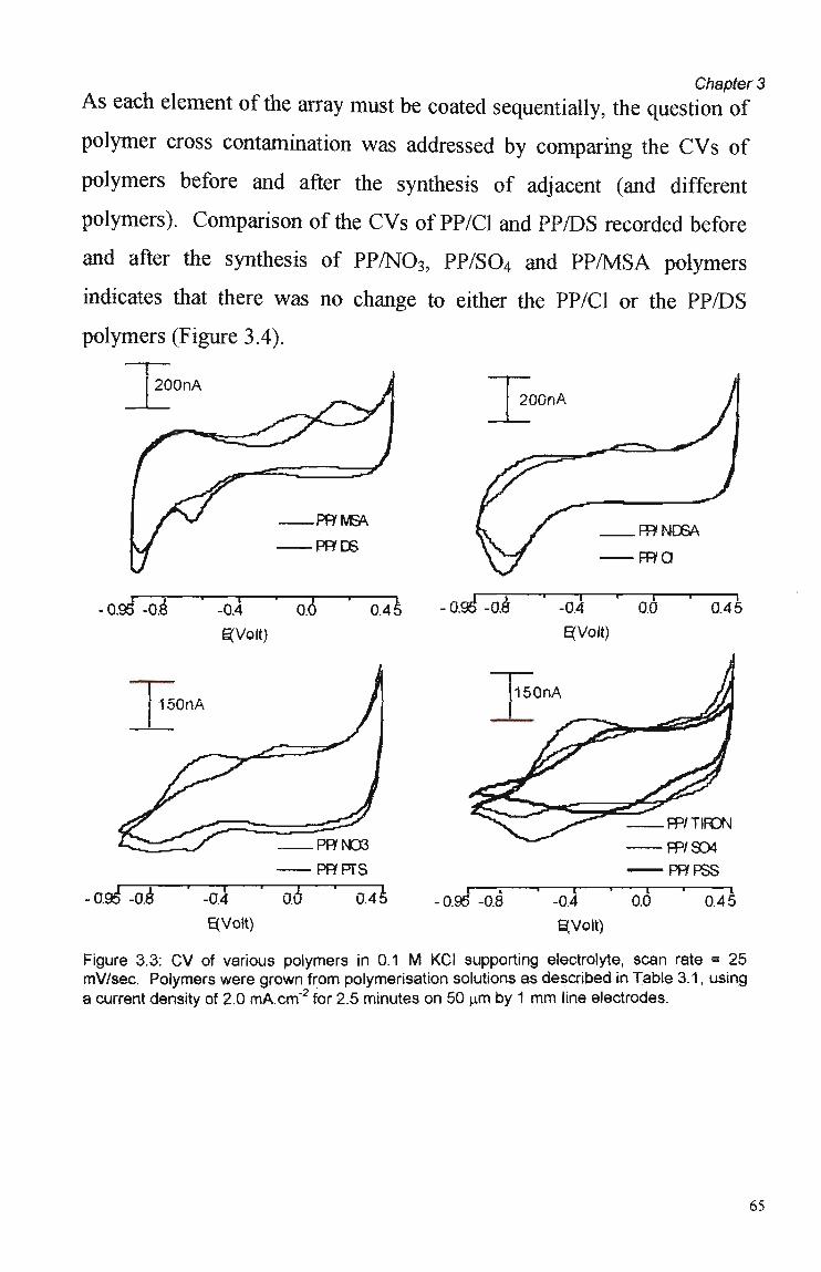
Chapter 3

A s each element of the array must be coated sequentially, the question of

polymer cross contamination was addressed by comparing the C V s of

polymers before and after the synthesis of adjacent (and different

polymers). Comparison of the C V s of PP/Cl and PP/DS recorded before

and after the synthesis of PP/N0 3 , PP/S0 4 and P P / M S A polymers

indicates that there was no change to either the PP/Cl or the PP/DS

polymers (Figure 3.4).

PP/MS<\

PFyrjs FP/Í^DGA

mo

- 0.951 -o.á 5T "ÒT ~ÕÃh -0.9 " -0.8 -0.4 — r 0.0

0.45

BíVolt) r^Volt)

PP/N03

PRfPTS

P?/TIRON

PP/S04

PP/PSS

0.9a -o.é -0.4

E(Volt) 3" 0 4 5 -0.9^" -0.8 -0.4

l^Volt)

~ão~ 1 0.45

Figure 3.3: C V of various polymers in 0.1 M KCI supporting electrolyte, scan rate = 25 mV/sec. Polymers were grown from polymerisation solutions as described in Table 3.1, using a current density of 2.0 mA.cm'2 for 2.5 minutes on 50 u m by 1 m m line electrodes.

65

Chapter 3

A

V i • ' i

3-0.8 -0.4

* • *

0.0

A-0.45

400nA

...before

after

r -0.95

r r u

-0.8

B

i |

-0.4

—

0.0

J

, n

0.45 E(Volt) E(Volt)

Figure 3.4: CV of (A) PP/Cl and (B) PP/DS polymers in 0.1 M KCf (scan rate = 25 mV.sec"1).

3.3.2 NAFION PRE-TREATMENT

The enhanced mass transport is one of the favourable properties of

microelectrodes (Section 1.4). However this same efficient mass

transport has the undesirable effect of carrying away a portion of the

soluble oligomers to the bulk solution before they can become insoluble

and be deposited onto the electrode surface. As electrode size decreases,

this effect becomes more pronounced and polymer deposition,

increasingly difficult. One manifestation of this phenomenon was an

increase in the growth potentials at smaller electrodes as discussed in

Section 3.3.1.4 above.

One strategy which did prove successful in improving the deposition of

polymer for some counterions was the application of a thin layer of

nafion to the lOum disc. This type of procedure has been described in a

review by Diaz and Lacroix112 (1988), as "two-step preparation" in which

an inert, insoluble host polymer film is applied to the electrode surface

prior to electrodeposition.

66

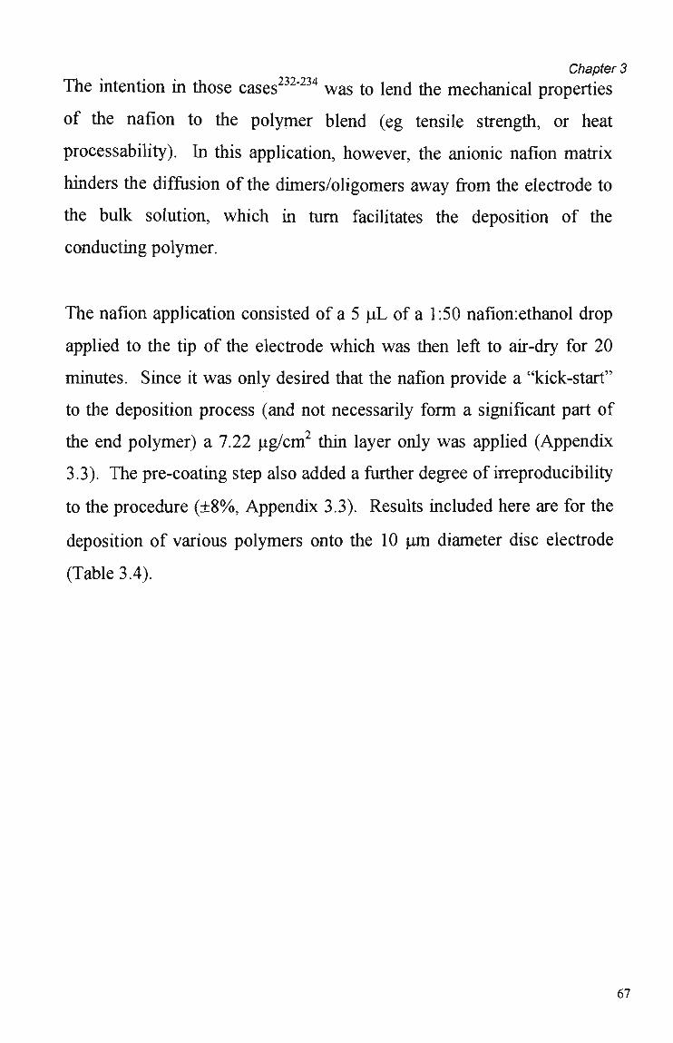
Chapter 3

The intention in those cases232"234 was to lend the mechanical properties

of the nafion to the polymer blend (eg tensile strength, or heat

processability). In this application, however, the anionic nafion matrix

hinders the diffusion of the dimers/oligomers away from the electrode to

the bulk solution, which in turn facilitates the deposition of the

conducting polymer.

The nafion application consisted of a 5 uL of a 1:50 nafion:ethanol drop

applied to the tip of the electrode which was then left to air-dry for 20

minutes. Since it was only desired that the nafion provide a "kick-start"

to the deposition process (and not necessarily form a significant part of

the end polymer) a 7.22 ug/cm thin layer only was applied (Appendix

3.3). The pre-coating step also added a further degree of irreproducibility

to the procedure (±8%, Appendix 3.3). Results included here are for the

deposition of various polymers onto the 10 u m diameter disc electrode

(Table 3.4).

67

There is NO p. 68 in original document

Chapter 3

A B

Figure 3.6: CVs in lO^M Na2S04, scan rate = 25 mV/sec, (A) = PP/NDSA; (B) = PP/NDSA/naf.

A B

Figure 3.7: CVs in lO^M Na2S04, scan rate = 25 mV/sec, (A) = PP/EBSA; (B) = PP/EBSA/naf.

A B

Figure 3.8: CVs in lO^M Na2S04, scan rate = 25 mV/sec, (A) = PP/4-SBA; (B) = PP/4-SBA/naf.

69

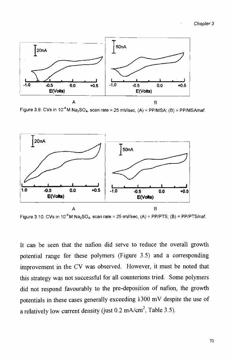
Chapter 3

|20nA

i k /t . i -10 -0.5 O.o

E(Volts)

i ,.. J •0.5

50nA

1 i . -1.0

_,1 i 1 ... -0.5 0.0 EfVolts)

+0.5

B Figure 3.9: CVs in lO^M Na2S04, scan rate = 25 mV/sec, (A) = PP/MSA; (B) = PP/MSA/naf.

•0.5 0.0

E(VoRs)

X -1.0 -0.5 0.0

E(Vofts) +0.5

A B

Figure 3.10: CVs in lO^M Na2S04, scan rate = 25 mV/sec, (A) = PP/PTS; (B) = PP/PTS/naf.

It can be seen that the nafion did serve to reduce the overall growth

potential range for these polymers (Figure 3.5) and a corresponding

improvement in the C V was observed. However, it must be noted that

this strategy was not successful for ali counterions tried. S o m e polymers

did not respond favourably to the pre-deposition of nafion, the growth

potentials in these cases generally exceeding 1300 m V despite the use of

a relatively low current density (just 0.2 m A / c m , Table 3.5).

70

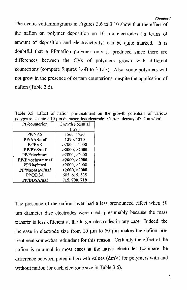
Chapter 3

The cyclic voltammograms in Figures 3.6 to 3.10 show that the effect of

the nafion on polymer deposition on 10 u m electrodes (in terms of

amount of deposition and electroactivity) can be quite marked. It is

doubtfül that a PP/nafion polymer only is produced since there are

differences between the C V s of polymers grown with different

counterions (compare Figures 3.6B to 3.10B). Also, some polymers will

not grow in the presence of certain counterions, despite the application of

nafion (Table 3.5).

Table 3.5: Effect of nafion pre-treatment on the growth potentials of various polypyrroles onto a 10 um diameter disc electrode. Current density of 0.2 mA/cm2.

PP/counterion

PP/NAS PP/NAS/naf PP/PVS

PP/PVS/naf PP/Eriochrom

PP/Eriochroin/naf PP/Naphthyl

PP/Naphthyl/naf PP/BDSA

PP/BDSA/naf

Growth Potential (mV)

1560, 1750 1390,1370

>2000, >2000 >2000, >2000 >2000, >2000 >2000, >2000 >2000, >2000 >2000, >2000 605, 615, 635 715, 700, 710

The presence of the nafion layer had a less pronounced effect when 50

pm diameter disc electrodes were used, presumably because the mass

transfer is less efficient at the larger electrodes in any case. Indeed, the

increase in electrode size from 10 pm to 50 u m makes the nafion pre­

treatment somewhat redundant for this reason. Certainly the effect of the

nafion is minimal in most cases at the larger electrodes (compare the

difference between potential growth values (AmV) for polymers with and

without nafion for each electrode size in Table 3.6).

71

Chapter 3

Table 3.6: Comparison of growth potentials with and without nafion for 10 um and 50 um electroc

Polymer

PP/PTS PP/Tiron PP/Chrom PP/4-SBA

es, with and without nafion pre

10 um, without nafion 840 340 1200 640

lOum with nafion 800 470 655 600

A m V for lOum

-40 +130 -545 -40

-treatment. 50um without nafion 720 500 750 600

50u,m with nafion 725 500 550 600

A m V for 50um

+5 0

-200 0

In particular, note the direction and magnitude of the A m V for

chromazurol and tiron counterions for the 10 u m disc electrode. W h y

should the nafion produce such dramatically different trends for these two

counterions?

If the growth potential is thought of as a measure of the ease of

deposition, then it would seem that the nafion pre-layer makes the

deposition of PP/chrom easier, while more energy (electrical potential) is

required for the deposition of PP/tiron through the nafion. That is not

unexpected, since the growth potential for PP/tiron (without nafion) is so

low to begin with, that the nafion (intrinsically non-conductive) would

make deposition more difficult in that case.

In the case of the chromazurol, the deposition without nafion is

considerably more difficult to begin with so that the initial disadvantage

of additional nafion pre-layer resistance is ultimately outweighed by the

advantage of additional oligomer entrapment by nafion.

The nafion pre-treatment could not be applied to the array electrodes

because of the electrode's intolerance to organic solvents (the nafion

must be applied in an ethanol/lower aliphatic alcohols mixture).

72

Chapter 3

Attempts to grow a PP/nafion polymer without supporting electrolyte on

either a 10 um or 50 |im disc electrode were unsuccessful, even with a

pyrrole concentration of 0.5 M. Application of a 2 mA/cm2 current

produced a potential of more than 2.0 V, and while a current density of

0.2 mA/cm2 did result in a lower potential (Figure 3.11), no deposition

occurred as was evident from the CV, even after 10 minutes (Figure

3.12).

Figure 3.11: Chronopotentiogram recorded during unsuccessful deposition of PP/Nafion (from 0.5 M pyrrole solution only) using 0.2 mA.cm"2 for 10 minutes on 50 um disc electrode.

Jl00nA

-1.0 -0.5 0.0

EfVott»)

• +0.5

Figure 3.12: C V of a 50 \im disc electrode with nafion pre-coating after unsuccessful deposition, (showing no polymer) in 10"* M N a 2 S 0 4 solution (scan rate of 50 mV.sec"

1)

3.3.2. E L E C T R O D E C O V E R A G E A N D M O R P H O L O G Y .

Generally, visual inspection with a microscope was adequate to check

that the polymer coverage was complete and even (Figure 3.13), since

any problems with polymer deposition and/or coverage was immediately

apparent.

73

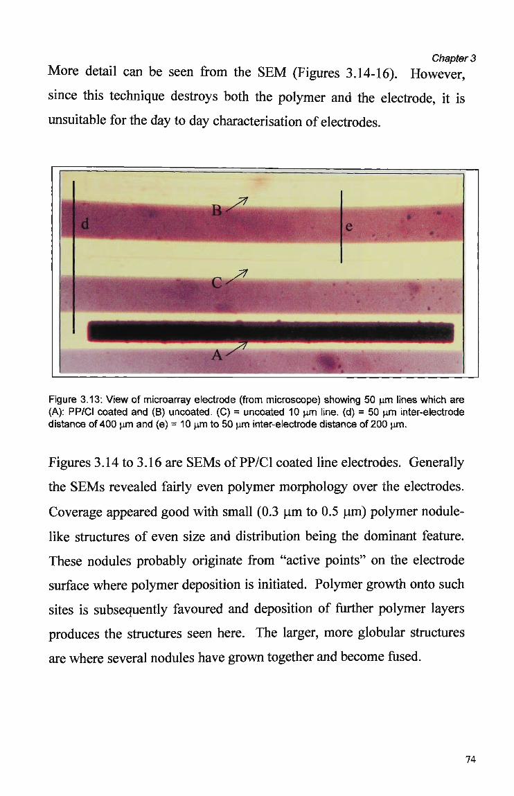
Chapter 3

More detail can be seen from the S E M (Figures 3.14-16). However,

since this technique destroys both the polymer and the electrode, it is

unsuitable for the day to day characterisation of electrodes.

Figure 3.13: View of microarray electrode (from microscope) showing 50 pm lines which are (A): PP/Cl coated and (B) uncoated. (C) = uncoated 10 pm line. (d) = 50 pm inter-electrode distance of 400 pm and (e) = 10 pm to 50 pm inter-electrode distance of 200 pm.

Figures 3.14 to 3.16 are S E M s of PP/Cl coated line electrodes. Generally

the S E M s revealed fairly even polymer morphology over the electrodes.

Coverage appeared good with small (0.3 u m to 0.5 u m ) polymer nodule-

like structures of even size and distribution being the dominant feature.

These nodules probably originate from "active points" on the electrode

surface where polymer deposition is initiated. Polymer growth onto such

sites is subsequently favoured and deposition of further polymer layers

produces the structures seen here. The larger, more globular structures

are where several nodules have grown together and become fused.

74

Figure 3.14: S E M of a section of PP/Cl deposited on a 50 pm line electrode.

Figure 3.15: S E M of a section of PP/Cl deposited on a 10 pm line electrode.

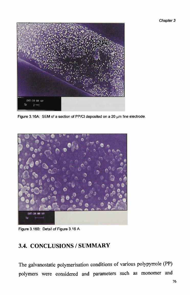
Chapter 3

Figure 3.16A: S E M of a section of PP/Cl deposited on a 20 pm line electrode.

Figure 3.16B: Detail of Figure 3.16 A.

3.4. CONCLUSIONS / SUMMARY

The galvanostatic polymerisation conditions of various polypyrrole (PP)

polymers were considered and parameters such as monomer and

76

Chapter 3

counterion concentration, current density and electrode size and shape

investigated.

The results of the nafion pre-treatment and its effects on the deposition of

different polypyrroles were interesting in their o w n right, even though it

was ultimately inappropriate (and unnecessary) for polymer deposition

onto microarray electrodes. The treatment proved advantageous in some

cases, but had no apparent effect in others. The reason for this is unclear,

but does suggest that the polymer produced in the presence of nafion are

not exclusively PP/nafion polymers. This is supported by the C V s of the

various PP/nafion/counterion polymers, in that they show distinct

differences that can only be attributed to the different counterions present

during polymerisation. It also emphasises the importance on the nature

of the counterion on the deposition of polypyrrole (ie that the deposition

efficiency is electrolyte dependent142).

Characterisation by CV and visual inspection (via light as well as

scanning electron microscopes) of the electrodes revealed that the

polymer deposition was reproducible under the polymerisation conditions

stated, and that polymer coverage of the electrodes was complete and

even in each case.

Importantly, there was no evidence of cross-contamination from one

polymerisation solution to another for polymers sequentially deposited onto

the array electrodes.

77

Chapter 4

CHAPTER 4

SIGNAL GENERATION

4.1 INTRODUCTION

The redox state and the ionic composition of conductive electroactive

polymers (CEP) are related, dynamic properties which respond to the

electrochemical stimulation of a polymer in the presence of some

supporting electrolyte (Section 1.3.1). W h e n the polymer is

electrochemically (or chemically) perturbed a current is produced, arising

from a number of possible sources including:

(i) the oxidation and reduction of the polymer itself,

(2) an increase or decrease in polymer conductivity,

(3) a change in the conductivity of the supporting electrolyte,

(4) flow of charging current due to fluctuations in the electrical potential

of a system,

(5) capacitive current, and

(6) the charge compensating ion movement into and out of the polymer

matrix.

Of these, the most selective is the current response due to ion movement

governed by polymer/analyte interactions. Ideally, it is this current

component which should be generated or maximised by the signal

generation mechanism so that the chemical discrimination capabilities of

the sensor are enhanced. At the very least, this component should

dominate the signal. A sensor whose response merely reflects (say)

analyte conductivity will not be much more selective or useful than a

conductivity detector!

Chapter 4

In addition, the method of signal generation should be such that ali

aspects of polymer selectivity may be exploited if so desired, be they

chemical, electrochemical, or kinetic in nature and origin.

4.2 EXPERIMENTAL

Polymer preparation and characterisation procedures and instrumentation

were as described in Section 2.1.1. with C V and chronoamperometric

procedures as outlined in Section 2.1.2. Supporting electrolytes, scan

rates and potential ranges for C V and chronoamperograms were as stated

in the text.

4.3 RESULTS AND DISCUSSION

4.3.1 CYCLIC VOLTAMMETRY

In Chapter 3, cyclic voltammetry (CV) was employed as a tool to assess

the reproducibility of polymer synthesis. However, the scanned potential

waveform can also probe polymer/ion interactions by highlighting

regions of the potential spectrum where the current produced is the

greatest (Section 1.5.1). The electroactivity of a number of different

polymers in different electrolytes can be assessed in this way (Figure

4.1).

79

Chapter 4

I—r •0.95

-I ' 1 ' 1 •0.4 0.0 0.45

I—r -0.95

— I ' 1 ' 1 -0.4 0.0 0.45

E(Volts) E(Volts)

I i • i • r •0.95 -0.4 0.0 0.45

E(Voits)

-0.95 ~l • T~ -0.4 0.0

E(Volts)

0.45

3 0 0 n A

l — i — ' i ' i ' i l r •0.95 -0.4 0.0 0.45 -0.95

E(Volts)

-0.4 0.0 0.45

E(Voits)

80

Chapter 4

G i i • i • r ^

•0.95 -0.4 0.0 — [ I—r 0.45 -0.95

-1 ' 1 ' í •0.4 0.0 0.45

E(Voíts) E(VoIts)

Figure 4.1 Cyclic voltammograms of various polypyrroles in 0.1 M potassium (green) and 0.1 M methylamine (red) supporting electrolytes (50 pm by 1 mm line electrode, grown at 2 mA/cm2 for 1.5 minutes from monomer/counteríon solutions listed in Table 2.1). Scan rate = 25 mV/sec. (A) = PP/PTS, (B) = PP/DS, (C) = PP/Cl, (D) = PP/MSA, (E) = PP/N03, (F) = PP/S04, (G) = PP/Tir, (H) = PP/NDSA, (t) = PP/PSS.

It is recognised that the size of the counterion is an important factor

contributing to the nature of the ion exchange of a polymer/supporting

electrolyte system235'236 (Section 1.3.1). However this behaviour is not

determined solely on the basis of counterion size, as was demonstrated

when the redox potentials of the polymers in two supporting electrolytes

were compared. If these values are thought of as measures of the

electrical potential energy at which ion movement occurs in each

polymer, then they may be used to compare ion exchange behaviours.

Table 4.1 lists the redox values from the C V s of a series of polymers in

potassium and methylamine electrolytes (data taken from Figure 4.1). 81

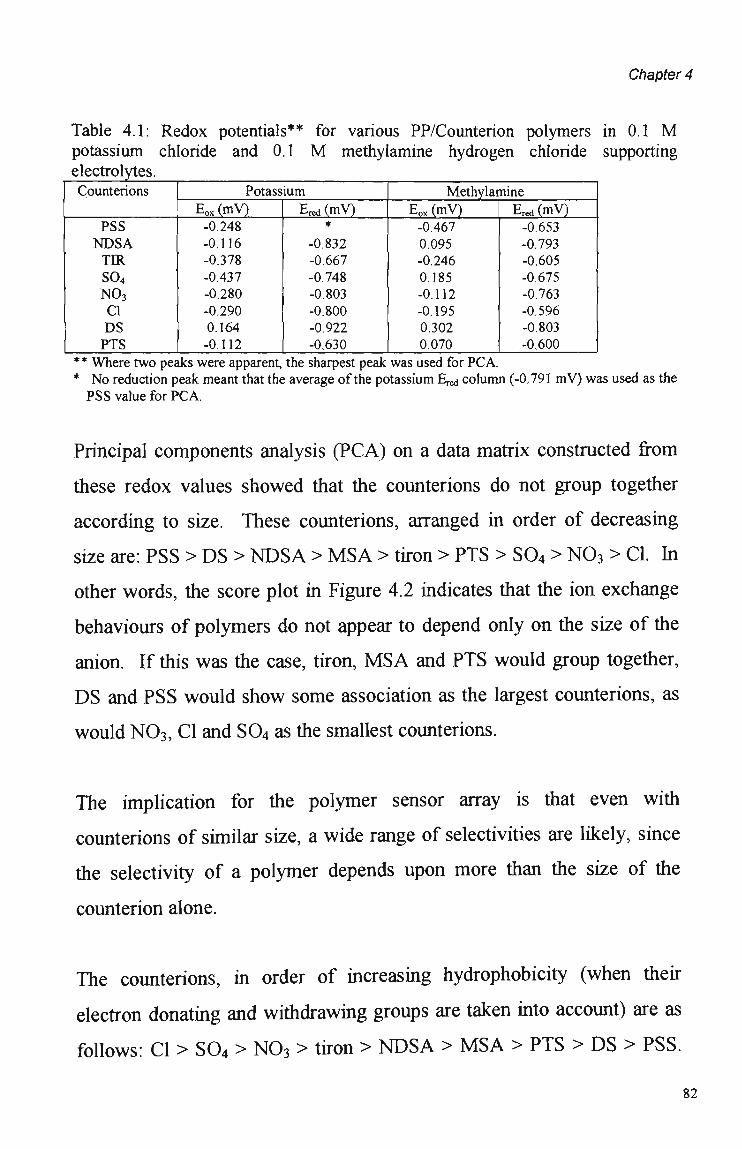
Chapter 4

Table 4.1: Redox potentials** for various PP/Counterion polymers in 0.1 M potassium chloride and 0.1 M methylamine hydrogen chloride supporting electrolytes. Counterions

PSS N D S A TIR S04 N03

Cl DS PTS

Potassium

Eox(mV)

-0.248 -0.116 -0.378 -0.437 -0.280 -0.290 0.164 -0.112

EredOnV) *

-0.832 -0.667 -0.748 -0.803 -0.800 -0.922 -0,630

Methylamine

Eox(mV)

-0.467 0.095 -0.246 0.185 -0.112 -0.195 0.302 0.070

Ered (mV) -0.653 -0.793 -0.605 -0.675 -0.763 -0.596 -0.803 -0.600

** Where two peaks were apparent, the sharpest peak was used for PCA. * No reduction peak meant that the average of the potassium E ^ column (-0.791 m V ) was used as the PSS value for PCA.

Principal components analysis (PCA) on a data matrix constructed from

these redox values showed that the counterions do not group together

according to size. These counterions, arranged in order of decreasing

size are: PSS > D S > N D S A > M S A > tiron > PTS > S 0 4 > N 0 3 > Cl. In

other words, the score plot in Figure 4.2 indicates that the ion exchange

behaviours of polymers do not appear to depend only on the size of the

anion. If this was the case, tiron, M S A and PTS would group together,

D S and PSS would show some association as the Iargest counterions, as

would N 0 3 , Cl and S 0 4 as the smallest counterions.

The implication for the polymer sensor array is that even with

counterions of similar size, a wide range of selectivities are likely, since

the selectivity of a polymer depends upon more than the size of the

counterion alone.

The counterions, in order of increasing hydrophobicity (when their

electron donating and withdrawing groups are taken into account) are as

follows: Cl > S 0 4 > N 0 3 > tiron > N D S A > M S A > PTS > D S > PSS.

82

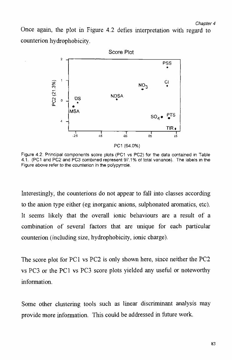
Chapter 4

Once again, the plot in Figure 4.2 defies interpretation with regard to

counterion hydrophobicity.

Score Plot

PSS

NOo •

NDSA

so4. P.TS

TIR» T 1 1 V

-25 45 «5 05 15

PC1 (64.0%)

Figure 4.2: Principal components score plots (PC1 vs PC2) for the data contained in Table 4.1. (PC1 and PC2 and PC3 combined represent 97.1% of total variance). The labels in the Figure above refer to the counterion in the polypyrrole.

Interestingly, the counterions do not appear to íàll into classes according

to the anion type either (eg inorganic anions, sulphonated aromatics, etc).

It seems likely that the overall ionic behaviours are a result of a

combination of several factors that are unique for each particular

counterion (including size, hydrophobicity, ionic charge).

The score plot for PCI vs PC2 is only shown here, since neither the PC2

vs P C 3 or the P C I vs P C 3 score plots yielded any useful or noteworthy

information.

Some other clustering tools such as linear discriminant analysis may

provide more information. This could be addressed in future work.

CO

CN

CN f •>

83

Chapter 4

4.3.2 C H R O N O A M P E R O M E T R I C S T U D I E S

Certainly a scanned potential waveform may be applied to a CEP sensor

in a ílow cell to induce controlled ion movement and produce a signal,

just as is done in a stationary cell with cyclic voltammetry. However,

variations in the rates of ion uptake and expulsion between polymers and

analytes is hidden with a scanned potential waveform, because the

kinetics of ion exchange within the polymer are dependent on the redox

state. If this redox state itself is in tlux (as with a scanned waveform)

then the increase and subsequent decay of current (for a particular redox

state) is obscured and cannot be measured. A pulsed waveform is most

appropriate if the extraction of certain kinetic information is desired.

Another consideration in choosing a waveform is that the electrochemical

manipulation of the polymer in the ílow cell must be rapid (one

oscillation over a period of anywhere between tens of milliseconds

(msecs) to a few seconds),. This is due to the sample plug in flow

injection analysis having a limited residence time in the electrochemical

flow through cell.

There are other practical difficulties with scanned potential waveforms

which are not encountered with pulses. Each current sample time along

the scan equates with a different potential which makes comparison of

diíferent scans and sample times difficult. This especially true when w e

consider that the scan rate must be adjusted according to the upper and

lower scan limit, to maintain the same sampling rate throughout. To

avoid these difficulties a pulsed waveform was favoured. The method of

Chapter 4

signal generation using the pulsed potential waveform may be

summarised in Figure 4.3. The mechanism outlined in this figure,

suggests that there are a number of ways of influencing polymer

selectivity when using this type of signal generation procedure.

The first involves changing the chemical composition of the polymer

itself, thereby altering the ion exchange behaviour of the sensor (Figure

4.3a). The second involves the manipulation of the pulsed potential

and/or the current sample point parameters (Figure 4.3b) to produce

chronoamperograms of different relative analyte selectivities (Figure

4.3c).

Chronoamperometric (current/time profile) studies were useful in

exploring these parameters. Parameters that may be "tuned" to

manipulate selectivity include polymer composition, upper and lower

pulsed potential limits (Ei and E2) and current sample time (csp). The

effect of these factors on the chronoamperograms produced was

examined.

85

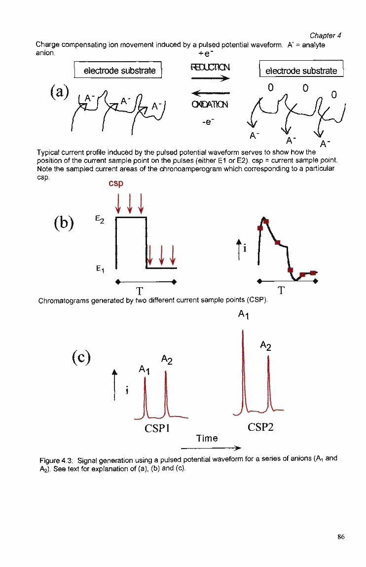
Chapter 4 Charge compensating ion movement induced by a pulsed potential waveform. A" = analyte anion. + e~

electrode substrate electrode substrate EHXCT1CN >

^

OCATCN

A- A-Typical current profüe induced by the pulsed potential waveform serves to show how the position of the current sample point on the pulses (either E1 or E2). csp = current sample point. Note the sampled current áreas of the chronoamperograrn which corresponding to a particular csp.

csp

(b) | j |

Hl

Chromatograms generated by two different current sample points (CSP).

Al

(c) A 2

CSP1 CSP2 Time

Figure 4.3: Signa! generation using a pulsed potential waveform for a series of anions (Ai and A2). See text for explanation of (a), (b) and (c).

86

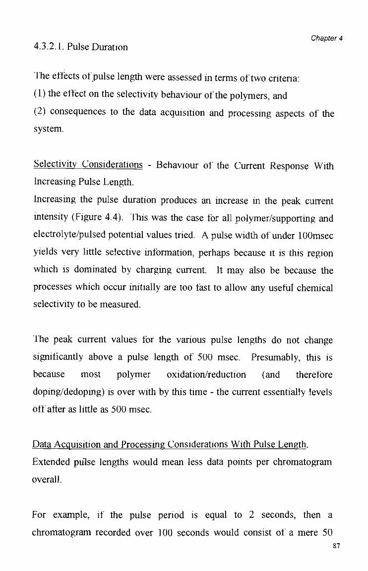
4.3.2.1. Pulse Duration Chapter 4

The effects of pulse length were assessed in terms of two cntena:

(1) the effect on the selectivity behaviour of the polymers, and

(2) consequences to the data acquisition and processing aspects of the

system.

Selectivity Considerations - Behaviour of the Current Response With

Increasing Pulse Length.

Increasing the pulse duration produces an increase in the peak current

intensity (Figure 4.4). This was the case for ali polymer/supporting and

electrolyte/puised potential values tried. A pulse width of under lüümsec

yields very little selective information, perhaps because it is this region

which is dominated by charging current. It may also be because the

processes which occur initially are too fast to allow any useful chemical

selectivity to be measured.

The peak current values for the various pulse Iengths do not change

significantly above a pulse length of 500 msec. Presumably, this is

because most polymer oxidation/reduction (and therefore

doping/dedoping) is over with by this time - the current essentially leveis

off after as little as 500 msec.

Data Acquisition and Processing Considerations With Pulse Length.

Extended pulse Iengths would mean less data points per chromatogram

overall.

For example, if the pulse period is equal to 2 seconds, then a

chromatogram recorded over 100 seconds would consist of a mere 50

Chapter 4

data points since one current sample would be taken every 2 seconds. It

is clear that longer pulse periods are unfavourable for this reason.

A pulse length of around 500 msec was adequate to satisfy both

selectivity and data acquisition criteria. Consider that if a minimum of

one current sample point is extracted from each pulse, then this

corresponds to a minimum extracted data sample rate of one data point

per second. Given that each peak takes approximately 25 to 80 seconds

to elute (see Figure 5.1), then each extracted peak will contain a

minimum of between 25 to 80 data points.

88

r~ o.o Time (seconds)

Chapter 4

0.1 0.2

0.0 - r -

0.2

40-i

0-

-20 -1

- 1 0.4

1 1 1 1 1 1 0.0 0.2 0.4 0.6 0.8 1.0

Time (seconds)

T 2 3

l

4

Time (seconds)

Figure 4.4: A comparison of the increasing current magnitudes resulting from the increase in pulse Iengths for PP/DS (50 um by 1 m m line electrode, grown at 2 mA/cm2 for 1.5 minutes) pulsed in lO^M NaCl supporting electrolyte between E, = 0.25 V and E2 = -0.40 V.

89

Chapter 4

csp -f-

Fígure 4.5 Pulsed potential waveform showing how a longer pulse period will result in a lower current sampling rate. T = pulse period, E^ and E 2 = upper and lower potential values respectively (switching potentials), cps = current sample point.

4.3.2.2 Pulsed Potential Range

Differences in the potential value at which ion incorporation/expulsion

occurs for different polymers and analytes may be exploited, and is

somewhat analogous to the more conventional detection of electroactive

metal ions through control of the applied potential. Chronoamperometry

with polymer coated electrodes shows h o w this electrochemical aspect of

polymer selectivity m a y be tuned simply by the selection of appropriate

pulsed potential values, as is shown in the example below (Figure 4.6).

This facilitates an in-situ method of tuning polymer selectivity which

commercial instruments do not offer (eg e-Nose from Neotronics, * and

others based on resistometric principies, see Table 1.1).

90

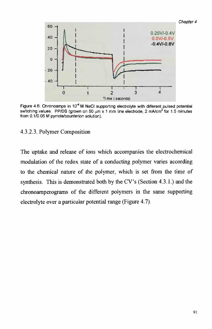
60 -

40 -

20 -

0 -

-20-

- 40 -

1

{

l t

1 i t

i 1

~T 0 1

I

1 } 1 í

"—— 1 • • i

1 J

i 1 1 ! 2 3

Ti me (seconds)

0.25V/-0.4V 0.0V/-0.5V -0.4V/-0.8V

1 4

Chapter 4

Figure 4.6: Chronoamps in lO^M NaCl supporting electrolyte with different pulsed potential switching values. PP/DS (grown on 50 um x 1 m m line electrode, 2 mA/cm2 for 1.5 minutes from 0,1/0.05 M pyrrole/counterion solution).

4.3.2.3. Polymer Composition

The uptake and release of ions which accompanies the electrochemical

modulation of the redox state of a conducting polymer varies according

to the chemical nature of the polymer, which is set from the time of

synthesis. This is demonstrated both by the C V s (Section 4.3.1.) and the

chronoamperograms of the different polymers in the same supporting

electrolyte over a particular potential range (Figure 4.7).

91

Chapter 4

Time (seconds)

Figure 4.7: Chronoamperograms for several polymers in lO^M NaCl, E, = 0.0 V and E2 = 0.8 V (50 um by 1 m m electrodes grown at 2 mA/cm2 for 1.5 minutes from solutions listed in Table 2.1).

4.3.2.4 Kinetic Effects

Different rates of ion incorporation and expulsion are evident in the

chronoamperograms of different polymers in various supporting

electrolytes (Figure 4.7). Shifting the current sample point (csp) along

the potential pulse changes the observed selectivity of the sensor.

Examples of the utilisation of these kinetic effects were demonstrated in

the flow cell by pulsed amperometric detection of a series of anions and

cations after ion chromatography in Section 5.3.3.

4.3.3 COMPETITION EFFECTS

Of the possible currents identifíed in Section 4.1 which can combine to

produce the signal, some are less desirable than others because they are

not selective. Currents which arise due to analyte conductivity and to

charging current are not based on the chemical nature of the analyte.

92

Chapter 4

Therefore chemical discrimination based on these currents is impossible.

Sampling later in the pulse (csp > 50 msec) avoids charging currents.

The suppression of the eluent (Appendix 2.2) is disadvantageous from a

selectivity perspective since low background conductivity produces a

relatively large change in solution conductivity upon the passage of the

analyte plug. With low background conductivity (less than 5 uS, see

Table 2.2), analyte conductivity would represent a greater proportion of

the signal generated, perhaps even screening any chemical selectivity.

However, suppression does reduce (if not eliminate) the incorporation of

competing eluent ions over the incorporation of analyte ions. Also,

eluent suppression brings the p H to close to neutral, which is a more

favourable environment for the polymer than the extremes of p H

experienced with the unsuppressed eluents.

4.3.4. POLYMER STABILITY IN SUPPRESSED ELUENTS.

The use of suppressed eluents raises the issue of the stability of CEPs in

low supporting electrolyte concentrations. Note the ion exchange (and

therefore the redox) behaviour of the polymer depends on the availability

of the ions in solution.

In order to determine the effect of the supporting electrolyte

concentration on electrode stability, a series of C V experiments were

performed in the various media over 1-2 hours. To ensure that the effect

of media conductivity (or ionic concentration) was studied and not the

chemical composition of the supporting electrolyte, NaCl solutions only

Chapter 4

were used. This salt maintains an essentially neutral p H when dissolved,

regardless of concentration, and consists of monovalent anions and

cations which are unlikely to be excluded from the polymer on the basis

of charge or size.

The experiments involved the continuous cycling of PP/Cl in media of

varying NaCl concentration (and therefore conductivity). The

electroactivity of the polymers after various cycling times in the different

solutions were assessed by C V in IO"2 M NaCl solutions. Note that the

experiments were performed in a two electrode cell (where the Pt mesh

auxiliary was also the reference electrode) so as to prevent leaching from

a NaCl filled reference/salt bridge.

CEP coated 10 um Pt disc electrodes were used to keep to an absolute

minimum detrimental electrochemical effects such as iR drop

experienced with larger electrodes in poorly conducting solutions

(Section 1.4).

The CVs in 10"2M NaCl (after 0, 40, 80 and 100 minutes cycling in the

various NaCl concentrations) are shown in Figure 4.8. Note that the C V s

recorded are the stable (unchanging) responses of the polymers in the 10"

M médium scanned at 50 mV/sec (though the polymers were scanned in

the low concentration solutions at a scan rate of 10 mV/sec).

94

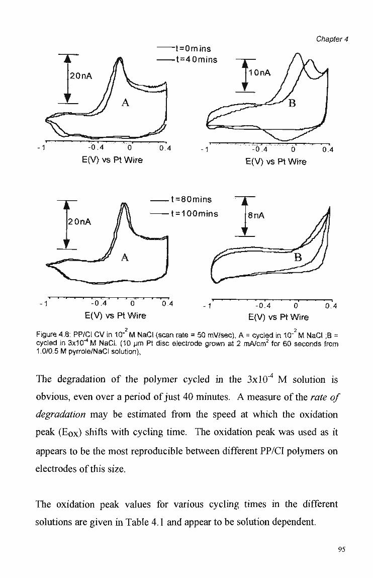
E(V) vs Pt Wire

t=Omins t=40mins

'-. * *- ' ...s.. i • • » i

-0.4 0 0.4 -1

Chapter 4

'~.-!.,...• •_._..» . L ..K •' • I

-0.4 0 0.4

E(V) vs Pt Wire

t=80mins

t = 100mfns

•~ i - — i . i

-0.4 n. ....ti .J r i -i

0 0.4 -1 E(V) vs Pt Wire

•0.4 • • — i

0.4

E(V) vsPtWrre

Figure 4.8: PP/Cl CV in 1Q" M NaCl (scan rate = 50 mWsec), A = cycled in 10" M NaCl ;B = cycled in 3x10"4 M NaCJ. (10 um Pt disc electrode grown at 2 mA/cm2 for 60 seconds from 1.0/0.5 M pyrrole/NaCI solution),

The degradation of the polymer cycled in the 3x10"4 M solution is

obvious, even over a period of just 40 minutes. A measure of the rate of

degradation may be estimated from the speed at which the oxidation

peak (Eox) shifts with cycling time. The oxidation peak was used as it

appears to be the most reproducible between different PP/CI polymers on

electrodes of this size.

The oxidation peak values for various cycling times in the different

solutions are given in Table 4.1 and appear to be solution dependent.

95

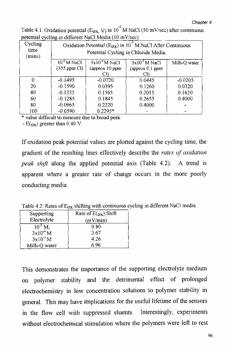
Chapter 4

Table 4.1: Oxidation potential (E0x, V ) in 10 M NaCl (50 mV/sec) after continuous

potential cycling in different NaCl Media (10 mV/sec).

Cycling time (mins)

0 20 40 60 80 100

Oxidation Potential (E0x) in 10 M NaCl After Continuous

Potential Cycling in Chloride Media.

IO"2 M NaCl (355 ppm Cl)

-0.1495 -0.1590 -0.1335 -0.1285 -0.0965 -0.0590

3x10^ M NaCl (approx 10 ppm

Cl) -0.0720 0.0395 0.1565 0.1845 0.2220 0.2295*

3xl0'5 M NaCl (approx 0.1 ppm

Cl) 0.0445 0.1260 0.2015 0.2655 0.4000

Milli-Q water

-0.0205 0.0320 0.1620 0.4000

* value difficult to measure due to broad peak - E(0x) greater than 0.40 V.

If oxidation peak potential values are plotted against the cycling time, the

gradient of the resulting lines effectively describe the rates of oxidation

peak shift along the applied potential axis (Table 4.2). A trend is

apparent where a greater rate of change occurs in the more poorly

conducting media.

Table 4.2: Rates of E0x shifting with continuous cycling in different NaCl media.

Supporting Electrolyte

10"2M, 3x10^M 3xlO-5M

Milli-Q water

Rate of E(ox) Shift

(mV/min) 0.80 3.67 4.26 6.96

This demonstrates the importance of the supporting electrolyte médium

on polymer stability and the detrimental effect of prolonged

electrochemistry in low concentration solutions to polymer stability in

general. This m a y have implications for the useful lifetime of the sensors

in the flow cell with suppressed eluents. Interestingly, experiments

without electrochemical stimulation where the polymers were left to rest

96

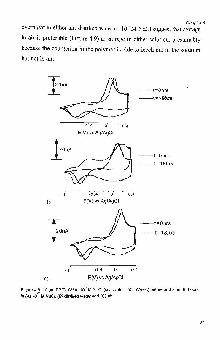
Chapter 4

overnight in either aü\ distilled water or 10'2M NaCl suggest that storage

in air is preferable (Figure 4.9) to storage in either solution, presumably

because the counterion in the polymer is able to leech out in the solution

but not in air.

-1 -0.4 0.4 E(V) vs Ag/AgCI

t=0hrs

-í=IShfs

-t=0frrs

-t=18hrs

B

20nA

-0.4 0

E(V) vs Ag/AgCI 0.4

•t=0hrs

t=18hrs

-1 -0.4 0 0.4

E(V)vsAg/AgCl

-2 Figure 4.9:10 um PP/Cl CV in 10 M NaCl (scan rate = 50 mV/sec) before and after 18 hours

in (A) 10'2 M NaCi, (S) dístiUed water and (C) air

97

Chapter 4

4.4 SUMMARY AND CONCLUSION

By inducing the controlled incorporation and expulsion of ions

throughout the polymer matrix, the inherent chemical affínity of any

polymer/analyte system may be exploited. This is achievable with either

scanned or pulsed potential waveforms though it was found that the

pulsed potential waveforms were most appropriate for extracting kinetic

information.

The chemical, electrochemical and kinetic selectivities of CEP sensors

were examined by chronoamperometry. These studies showed that the

pulsed signal generation waveform is most appropriate for electroinactive

anion and cation detection.

A rapid pulsed potential waveform allows:

(1) the rapid and continuous regeneration of the polymer matrix after it

has been exposed to an analyte plug,

(2) an adequate sampling rate to be maintained and

(3) the ability to "tune" the electrochemical and kinetic detection

parameters and selectivities.

The use of this signal generation waveform in the flow cell, for the pulsed

amperometric detection of a series of anions and cations, separated by ion

chromatography is the subject of Chapter 5.

98

Chapter 5

CHAPTERS

BEHAVIOUR OF POLYPYRROLE SENSORS IN A

FLOW CELL - THE DETECTION OF ANIONS

AND CATIONS AFTER ION

CHROMATOGRAPHY.

5.1: INTRODUCTION

In Chapter 4, the method of signal generation was such that the different

aspects of polymer selectivity could be accessed. The principie is sound -

measure current fluctuatíons that aríse due to the electrochemical

inducement of ion exchange of eluent and analyte ions (as discussed in

Chapter 4). The selectivity can be controlled by utilising the chemical

nature of the polymer, the appropriate potential range and/or the current

sampling point.

In this chapter, these aspects are explored in the flow cell under

chromatographic conditions for anions and cations. In this way the

"tunable" nature of polymer selectivity was demonstrated.

5.2: EXPERIMENTAL

Table 5.1 lists polymers used and synthesis solutions. Ali polymers were

grown galvanostatically using 2 m A / c m 2 current density, with growth

times are as stated in the text.

Chapter 5

Polymer synthesis and C V instrumentation were as for Section 2.1.1.

Chromatographic conditions were as given in Table 2.2, Section 2.2.1.

Preparation of anion and cation standard mixtures as for Section 2.2.1.1.

Table 5.1 Iísts polymers used, monomer/counterion concentrations.

Table 5.1 ... .,

Polymer

PP/Cl

PP/S04

PP/NO3 PP/DS PP/MSA

Monomer/Counterion Concentrations (M)

0.5/1.0 0.5/1.0 0.5/1.0

0.5/0.1 0.1/0.05

Flow cell and FIPLC Iayout were as described in Section 2.2.1.2.

Pulsed potential waveforms were used as described in text (with pulse

period = 1 second).

Data collection and processing procedures were as described in Section

2.3.2.1.

5.3: RESULTS AND DISCUSSION

5.3.1: POLYMER COMPOSITION

The selection of the counterions incorporated into the polymer electrode

was not determined solely on the basis of the chemical properties

possessed by these molecules, but also by the ease and reproducibility of

100

Chapter 5

polymer synthesis. These two considerations were of prime importance as

they restricted the selection of counterions somewhat (Section 3.3.1.1).

The polymers used here and their synthesis conditions are listed in Table

5.1. Responses to a series of anions and cations separated by ion

chromatography were investigated using select electrochemical conditions.

The effects of electrochemical manipulation are discussed in later sections

(Sections 5.3.2 and 5.3.3). This waveform is by no means "optimal" as

far as either selectivity or sensitivity are concerned, but does show the

importance of polymer composition in influencing both of these

properties.

The strategy of changing chemical composition to produce different

polymer selectivities was successful. This is obvíous from the responses

of these polymers to a series of the same ions (Figures 5.1 and 5.2).

The peak heights for the anion and cation responses in Figures 5.2 and 5.3

are given in table form below (Table 5.2). The data represents the peak

heights for the different polymers and analytes, whereas a measure of the

various relative selectivities of the polymers is given by the peak ratios

(Table 5.3, see Appendix 5.1).

101

Chapter 5

Table 5.2: Peak Responses of Various Polymers To A Series of Anions and Cations, Electrochemical Detection Parameters - Ei = 0.00 V, E 2 = 0.25 V, Current Sample Point =100 msec on E2.

Analyte

Li Na NH4 K Mg Ca F Cl S04 N03

P04

Peak Height (nA) PP/Cl

18.82

34.12 1 58.82

42.35 1 22.35 24.12 24.12 22.27 47.27 32.73 20.00

PP/S04

4.21 6.05 1 11.58 7.63

0.53 -1.58 ----

-

PP/NO3

2.78 4.56 4.77 5.44 2.89 3.55 2.57 2.71

7.00 4.57 2.71

PP/DS

15.79 30.53 50.53 38,95 22.11 25.26 25.55 25.55 58.89 38.89 23.33

PP/MSA

17.33 40.00 65.33 56.00 -4.00 -6.67 13.75 14.38 31.88 30.00 13.13

- unable to measure due to poor or ambiguous peak shape (see Figure 5.2). Analyte concentrations were as for Figure 5.1 and 5.2.

Table 5.3: Peak response ratios of various polymers to a series of anions and cations electrochemical detection parameters - E] = 0.00 V, E 2 = 0.25 V, Current Sample Point =100 msec on E2. (data from Figures 5.1 and 5.2).

Analytes

Na/Li NHVLi 1 K/Li Mg/Li Ca/Li Cl/F SO4/F NO3/F

H2PO4/F

Peak Ratios*

PP/Cl

f 1.81 3.13 2.25

1.19 1 1.28 1.04 2.21 1.53 0.94

PP/SO4 1.44 2.75 1

í 1.81 0.13 -0.38 -

-

-

-

r PP/NO3

1.64 1.72 1.96 1.04 1.28 1.05 2.72 1.78 1.05

PP/DS

1.93 3.20 2.47 1.40 1.60 1.00

[ 2.30 1.52 0.91

PP/MSA

2.31 3.77 3.23 -0.23 -0.38 1.05 2.32 2.18 0.95

- no measurable peaks (peak shape too poor or ambiguous). *Peak ratios calculated from responses in Figures 5.1 and 5.2.

Chapter 5

5.0 nA

PP/ Cl

PP/ M0 3

PP/ MSA

PP/ so4

PP/DS

Figure 5.1: Cation Chromatography - Detection Parameters: 0.00 V to 0.25 V, Current Sample Point = TOO msec on E2. Peak (T) = T ppm Líthíum; (2) 4 ppm Sodium; (3) TO ppm Ammontum; (4) 10 ppm Potassium; (5) 5 ppm Magnesiurn; (5) 10 ppm Cálcium. Injection Toop = 50 uL. Retention times are as forTábfe 2.3.

103

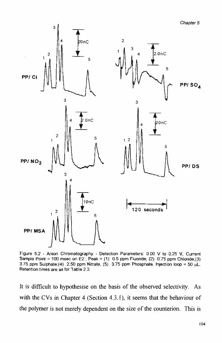
PP/Cl

Chapter 5

PP7N03

- jypf S Q 4

PP/DS

h 120 seconds

PP/MSA

Figure 5.2 - Anion Chromatography - Detection Parameters: 0.00 V to 0.25 V, Current Sample Point = 100 msec on E2.; PeaK = (T) 0.5 ppm Fluoride; (2) 0.75 ppm ChToride;(3) 3.75 ppm Sufphate;(4) 2.50 ppm Nitrate, (5) 3.75 ppm Phosphate. Tnjectíon loop = 50 IJL. Retention times are as for Table 2.3.

It ís difficult to hypothesíse on the basis of the observed selectivity. A s

with the CVs ín Chapter 4 (Section 4.3.1), it seems that the behaviour of

the polymer is not merely dependent on the size of the counterion. This is

104

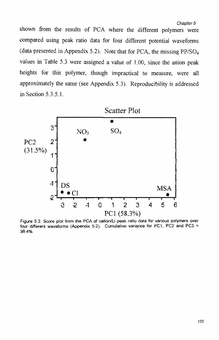
Chapter 5

shown from the results of P C A where the different polymers were

compared using peak ratio data for four different potential waveforms

(data presented in Appendix 5.2). Note that for PCA, the missing PP/SO4

values in Table 5.3 were assigned a value of 1.00, since the anion peak

heights for this polymer, though impractical to measure, were ali

approximately the same (see Appendix 5.3). Reproducibility is addressed

in Section 5.3.5.1.

ScatteT PJot

PC2 2" (31.5%)

0"

-r I I I I I I

0 1 2 3 4 5 6 PCI (58.3%)

Figure 5.3: Score plot from the P C A of caíion/U peak ratio data for various polymers over four different waveforms (Appendix 5.2>. Cumuiative variance for PCT, PC2 and PC3 -98.4%.

5 - 2 - 1

Chapter 5

Scatter Plot

PC2 (35.1%) r

T— •3

i

2 i

-1 — i i i r-

0 1 2 3 PCI (47.6%)

Figure 5.3: Principal Component Analysis of anhn^f peak ratio data for various polymers over four different waveforms (Appendix 5.3). Cumuiative variance for PCV, PC2 and PC3 94.1%.

These score plots indicate some sünilarity between the PP/CI and PP/DS

responses over the broad range of potentials used (Appendíces 5.2 and

5.3). W h y this should be ís not clear, since the counterions have very

different sizes and chemical natures. The P C A on the anion data showed

some similarity between P P / M S A and P P / N 0 3 responses.

The chromatograms in Figures 5.1 and 5.2, particularly those for PP/S0 4

serve to demonstrate the potential instability of the baseline responses of

CEPs. The low ionic strength of the suppressed eluent is the most likely

cause of the observed baseline instability. This chemical instability of

CEPs in solutions of low ionic strength has been investigated by C V and

is discussed in Section 4.3.4. One possible way to overcome the problem

of polymer instability due to low ionic strength would be to introduce

106

Chapter 5

some kind of ionic buffer to the eluent after the conductivity detector, and

have the sensor array placed downstream. However, due to the

competition effects described in Section 4.3.3, this would be likely to

dramatically decrease the sensitivity of the sensors.

5.3.2 ELECTROCHEMICAL PARAMETERS

This section consíders a single polymer composition (PP/CI) with a range

of electrochemical detection parameters investigated.

The peak ratio plots (Figure 5.4) show that the selectivity of the electrode

ís dependent on the upper and lower potential limits, and also on the

current sample point (csp) chosen.

107

Chapter 5

Figure 5.4: Ratios of aníon/F peak heights observed for PP/Cl over four different pulsed potential waveforms. Anion concentrations as for Figure 5.2.

5.3.3 C X f R R E r T T S A M P L E P O I N T

Figure 5.5 (A and B) illustrates selectivity behaviour expressed as peak

ratios relative to Lithium for cations or Fluoride for anions. Interestingly,

the behaviours of the divalent ions (both cations and anions Ca2+, M g 2 +

and S042') are similar according to these plots. This is also true for the

monovalent Na+, K+, Cl" and H 2 P 0 4 ' ions. In each case, the nitrogen

containing N O s and N H 4+ signals persist towards the end of the pulse.

108

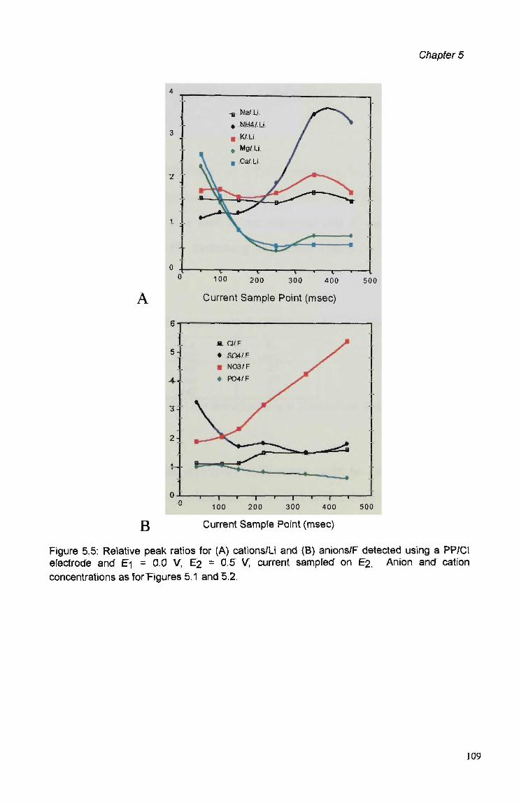
Chapter 5

500

Current Sample Point (msec)

B

M. rj/.F

• ,Sfí4/.F

• N03/F

« P04/F

— I — 100

—r~ 200

— I — 300 400

Current Sample Point (msec)

500

Figure 5.5: Relative peak ratios for (A) cations/Li and (B) anions/F detected using a PP/Cl electrode and Ei = 0.0 V, E2 = 0.5 V, current sampled on E2. Anion and cation concentrations as for Figures 5.1 and 5.2.

109

Chapter 5

5.3.4 EFFECT O F P O L Y M E R THICKNESS O N SELECTIVITY

B E H A V I O U R .

The cyclic voltammograms of PP/CI polymers ín NaCl supporting

electrolyte show variatíons between polymers of different thicknesses

(Figure 5.6). There ís a shift in the reduction and oxidation peaks with

increasing thickness (ie increasing deposition time), as shown ín Table

5.4.

Table 5.4: Redox potential values (mV) for PP/CI cycled ín 0.1 M NaCl (50 mV/sec)

Polymer Deposition Time

45 secs

90 secs 180 secs

Ered

(mV) -683 -650 -583

E 1 ^ox (mV)

-83 ! -67 í -283

Polymers erown from 1.0/0.5 M pyrrole/NaCl solution at 2 mA/cm2 on 50 u m x 1 m m ,gold line

electrodes.

This may indicate that selectivity differences could be expected between

polymers of different thicknesses. Note that of the three thicknesses, the

cyclic voltammograms of A and B appear to be most similar, with regard

to peak redox potentials (Ercd and Eox, Table 5.4). This ís interesting in

Iíght of the selectivity results shown in Figure 5.8.

The most obvíous change between ion chromatograms which occurs with

polymer thickness is the increase in the response obtained (Figure 5.7).

no

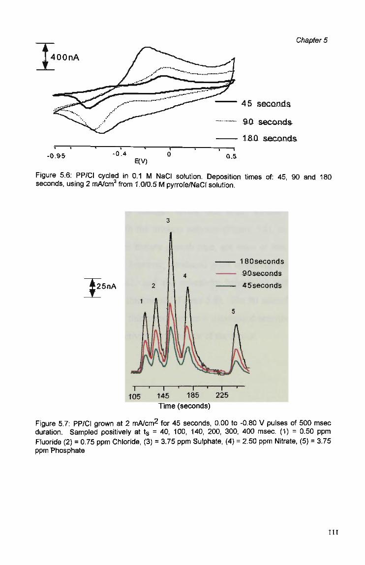
1 1

-0.4 E(V)

Chapter 5

45 seconds

&£ seconds

l&Q seconds

Figure 5.6: PP/Cl cycled in 0.1 M NaCl solution. Deposition times of: 45, 90 and 180 seconds, using 2 mA/cm2 from 1.0/0.5 R/T pyrrofe/NaCr sofutíon.

í 25nA

T T

180seconds

9-0-seco,nds

45seconds

T 105 145 185 225

Time (seconds)

Figure 5.7: PP/Cl grown at 2 mA/cm2 for 45 seconds, 0.00 to -0.80 V pulses of 500 msec duration. Sampled positively at ts = 40, 100, 140, 200, 300, 400 msec. (1) = 0.50 ppm Fluoride (2) = 0.75 ppm Chloride, (3) = 3.75 ppm Sulphate, (4) = 2.50 ppm Nitrate, (5) = 3.75 ppm Phosphate

III

Chapter 5

For sensitivity considerations, the thicker polymer m a y be desirable.

However a comparison of relative selectivity changes for the different

thicknesses indicate otherwise.

Figure 5.4 (Section 5.3.2) shows that the potential range which produced

the selectivity change of greatest magnitude was 0.0 V to -0.8 V. These

are also the potential limits between which most of the electroactivity

occurs, as can be seen from the C V (Figure 5.6).

The relative selectivity changes reveal that little "kinetic" selectivity

change ís apparent with the thickest polymer (Figure 5.8), as the curves

themselves for the three minute growth time, are more or less horizontal.

The thínner polymers, however, produced good selectivity changes over

the length of the pulse, and the selectivity behavíours were virtually

ídentícal for these two thicknesses (Figure 5.8). The 90 second deposition

time was the preferred thickness here, as ít maxímised sensitivity without

compromísing the selectivity performance of the sensor.

112

Chapter 5

Selectivities Relative to Fluoride.

B

-Cl/F •S04/F

. N03/F

- P04/F

^ * * ' ' • ,. . •

-T \ 1 \ 5 7 ! H

100 200 300 400

Current Sample Time (msec)

Figure 5.8: Ratios of peak heights (feft hand scafe, refatíve to fíuoride) for (A) 45 and 90 seconds growth time and (B) 180 seconds growth time for PP/Cl pulsed between O.OV and 0.25 V, sampíed on 0.25 V at 100 msec. Anion concentrations as for Figure 5.7.

The lack of relative selectivity changes in the thickest polymer (Figure

5.8B) could be indicative of a significant (non-selective) conductivity

component to the signal.

This is supported by two facts:

(1) The selectivity profíle does not change, suggestíng that a non-selectíve

current component domínates the signal and

&-. A

4 -•

3 -

s

1 -

i — ' — T — • — Í — ' — i — ' — r

0 100 200 300 400

4 i

3 -l

"\

113

Chapter 5

(2) the sensitivity series for the thicker polymer is the same as that for

conductivity detection, regardless of where along the pulse the current

is sampled (Table 5.5).

Table 5.5: Sensitivity series for PP/CI with different deposition times.

Electrochemical detection parameters were: Ej = 0.0 V. E 2 = 0.25 V, current sampled onE2. Current sample point (msec)

LQQ 250

[ 400

Selectivity series for 45 and 90 see deposition times

NOi>CL>S04>F>HaP04

N0 3 >a>S0 4 >F>H 2 P0 4

Na3>Cl>S04>F>H2PO4

Selectivity series for 180 see deposition times

S04>N01>CL>F>HaP04

S04>N03>CJ>F>H2P04

, S04>N03>C1>F>H2P04

Conducrivity seBsiúvky series = S04>NG3>Cl>F>H2PG4 Airkm conc&ráitíàor& as for Figure 5.7.

5.3.5: S E N S O R P E R F O R M A N C E

The reproducibility and analytical performance of the coated array

electrodes are investigated ín this section.

5.3.5.1 Reproducibility

In Chapter 3, polymer synthesis and reproducibility were investigated by

both cyclic voltammetry and visual inspection of the polymer coating.

Note that response reproducibility is also demonstrated ín the P C A s of

Section 6.3.1.2.

The reproducibility of 10 um x 1 mm and 50 um x 1 mm gold line arrays

were assessed here by the comparison of the performance of three PP/CI

electrodes of each size in the flow cell. These electrodes, when subjected

114

Chapter 5

to the same detection parameters and conditions did show that the 50 u m

electrodes were more reproducible than the 10 um (Table 5.6). This is

evident in the responses reproduced in Figure 5.9.

Table 5.6 Average peak heights and standard deviations for PP/Cl responses (see Figure 5.9). PP/Cl detection, potential pulsed between Ej = 0.50 V and E 2 =•• -0.50 V,

50 u m lines and 10 u m lines, cuiTent sample point = 440 msec on E2. Analyte

50um line

average ± SD %SD

lOumline average SD

1 % SD

Peak Height Fluoride (nA)

8.14 ±0.61 7.5%

1.02 ±0.28 27.2%

Peak Height Chloride (nA)

15.1 ±1.22 8.1%

2.4 ±0.27

11.1%

Peak Height Sulphate (nA)

Peak Height Nitrate (nA)

11.4 ±0.34 34.5 ±1.22 3.0% 3.5%

i 6.71 ±0.54 1 8.0%

- Peak too poor (compare with baseline) to measure. Anion concentration as for Figure 5.9. Standard deviation for 9 5 % confidence limits.

(i) 60 seconds

(ü)

Figure 5.9: Anion chromatograms - PP/Cl detection (1) 0.50 ppm Fluoride, (2) 0.75 ppm Chloride, (3) 3.75 ppm Sulphate, (4) 2.5 ppm Nitrate. Potential pulsed between E, = 0.50 V and E2 = -0.50 V, (I) 50 um x 1 m m lines and 10 um x 1 m m lines, current sample point = 440 msec on E2.

115

5.3.5.2 Analytical Performance Chapter 5

Calibration Curves

Conventional determination of electroinactive ion concentration after their

separation by ion chromatography is performed by conductivity

detection.229'230 Typical conductivity calibration curves for a series of

anions are shown in Figures 5.10 and 5.11. They show a linear response

with analyte concentration (over the 0.20 p p m to 20 p p m range tested) as

expected.

Cation Calibration Curves (Conductivity Detection)

2 4 6 8 10

Cation Concentration (ppm)

Cation Calibration Curves (Conductivity Detection)

Cation Concentration (ppm)

Figure 5.10: Cation Conductivity Calibration Curves.

116

Chapter 5

(Conductivity Detection)

1

Anion Concentration (ppm)

Anion Calibration Curves (Conductivity Detection)

2 4 6

Anion Concentration (ppm)

Figure 5.11: Anion Conductivity Calibration Curves.

It is not so simple when generating equivalent calibration curves for C E P

sensor responses because of the various detection parameters which affect

C E P sensor selectivity and sensitivity. With C E P sensors, chemical and

electrochemical parameters have to be defined.

The sensitivity and linearity of CEP sensor responses depend on the

chemical composition of the sensor. This is apparent from a comparison

117

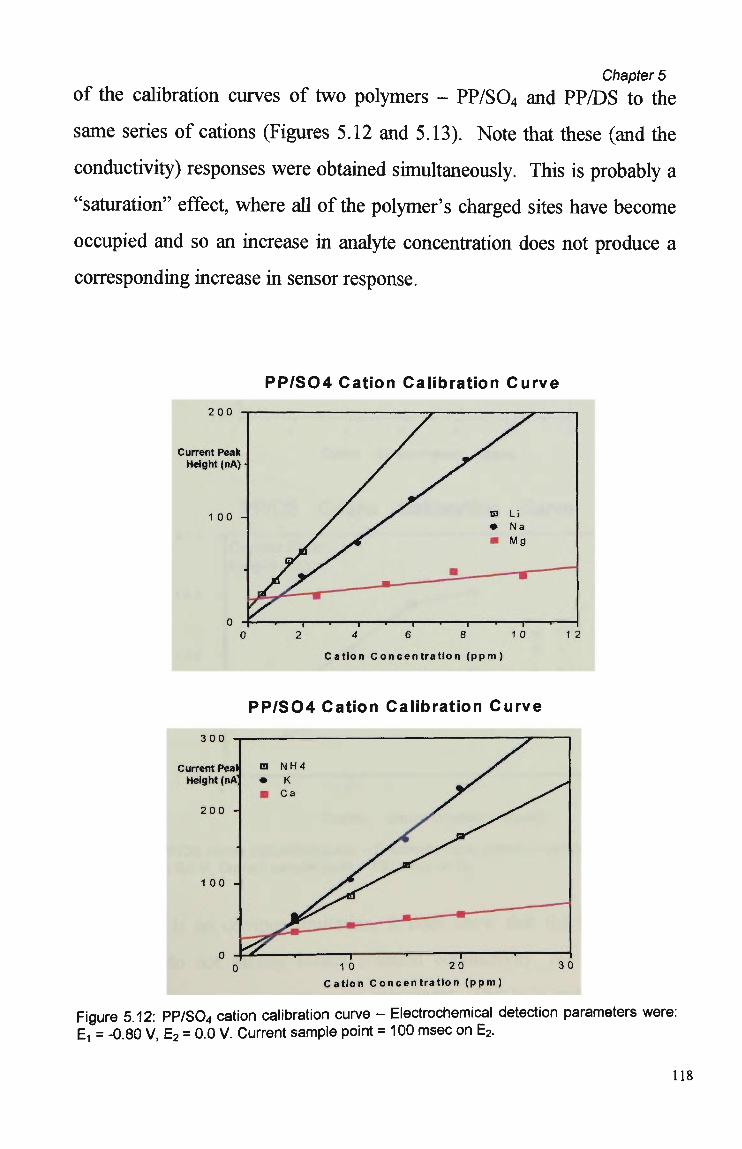
Chapter 5

of the calibration curves of two polymers - PP/S04 and PP/DS to the

same series of cations (Figures 5.12 and 5.13). Note that these (and the

conductivity) responses were obtained simultaneously. This is probably a

"saturation" effect, where ali of the polymer' s charged sites have become

occupied and so an increase in analyte concentration does not produce a

corresponding increase in sensor response.

PP/S04 Cation Calibration Curve

Current Peak Height (nA) •

1 0 0 -

0 2 4 1 1

6

• __

8

El Li • Na

• Mg

1 0 1 2

Cation Concentration (ppm)

PP/S04 Cation Calibration Curve

300

Current Peat Height (nA'

200 H

1 00 -

Cation Concentration (ppm)

Figure 5.12: PP/S04 cation calibration curve - Electrochemical detection parameters were: Ei = -0.80 V, E 2 = 0.0 V. Current sample point = 100 msec on E2.

118

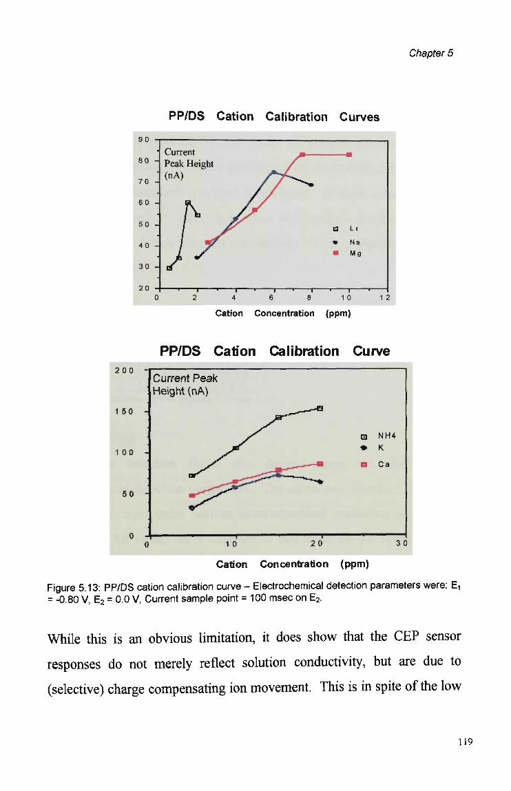
Chapter 5

PP/DS Cation Calibration Curves

90

80 -

70

60

Current Peak Height (nA)

• L i

* Na • Mg

—• r 4 6 8 10

Cation Concentration (ppm)

1 2

PP/DS Cation Calibration Curve 200 -f

1 50

1 00

50 -

Current Peak Height (nA)

• NH4 • K

a Ca

0 10 20 30

Cation Concentration (ppm)

Figure 5.13: PP/DS cation calibration curve - Electrochemical detection parameters were: E^ = -0.80 V, E 2 = 0.0 V, Current sample point = 100 msec on E2.

While this is an obvious limitation, it does show that the C E P sensor

responses do not merely reflect solution conductivity, but are due to

(selective) charge compensating ion movement. This is in spite of the low

119

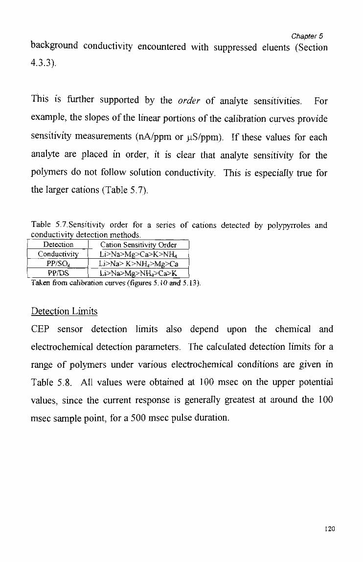
Chapter 5

background conductivity encountered with suppressed eluents (Section

4.3.3).

This ís further supported by the order of analyte sensitivities. For

example, the slopes of the linear portions of the calibration curves provide

sensitivity measurements (nA/ppm or jaS/ppm). If these values for each

analyte are placed in order, it ís clear that analyte sensitivity for the

polymers do not follow solution conductivity. This is especially true for

the larger cations (Table 5.7).

Table 5.7. Sensitivity order for a series of cations detected by polypyrroles and conductivity detection methods.

Detection Cation Sensitivity Order Conductivity Li>Na>Mg>Ca>K>NH4

PP/SQ4 LJ>Na> K>NH4>Mg>Ca \ PP/DS 1 Li>Na>Mg>NH4>Ca>K Taken from calíbrafioii curves {figures 5. 1Q and 5.13).

Detection Limits

C E P sensor detection limits also depend upon the chemical and

electrochemical detection parameters. The calculated detection limits for a

range of polymers under various electrochemical conditions are given in

Table 5.8. A H values were obtained at 100 msec on the upper potential

values, since the current response is generally greatest at around the 100

msec sample point, for a 500 msec pulse duration.

120

Chapter 5 Table 5.8 Calculated detection limits (ppb) for various polymers over different pulsed potential waveforms. Current sample point = 100 msec, sampled on upper potential value. Polymer/Waveform

0.0 V/0.5 v

1 PP/Cl L PP/SQ*

PP/N03

PP/DS PP/MSA

-0.4 V/-0.8 V PP/CI PP/SO4

pp/M03

PP/DS PP/MSA

-0.4 V/0.0 V PP/Cl

PP/SO» PP/NQj PP/DS PP/MSA

0.0 V/9.25 V PP/CV

PP/SG4* PP/NO3 PP/DS PP/MSA

Li

45 135 190 40 165

45 165 175 45 40

30 80 75 30 25

200 170 130 215 230

Na

JJ5 275 390

no 260

105 520 460 115 85

70 230 205 75 60

430 480 310 445 430

NR,

4J0 880 1-875 390 555

280 2140 1810 310 860

180 610 625 190 210

625 640 130 730 640

K

260 730 1110 240 590

200 1250 1035 220 190

155 450 470 165 120

910

Mg

J05 305 350 120 270

190 1665 790 180 600

90 470 315 100 210

885 1035 5000 650 880 770

625 830 5000

Ca

190 640 770 200 535

345 3335 1580 290 640

180 1185 625 1SS 410

1765

F

30 170 250 35 55

30 150 215 30 95

30 150 215 30 90

80

Cl

50 190 320 50 80

45 125 280 45 110

60 190 250 55 115

115

S04

75 350 590 330 125

70 290 390 70 190

80 310 400 90 165

265

N03

80 360 575 85 120

75 250 360 70 155

90 300 395 90 155

260 3000 >5O0 >750 >3750 >2500 1015 1365 1500

170 70 105

265 105 140

490 225 310

520 230 225

H2PO4 |

240 1410 1875 255 400

215 940 1250 210 590

215 865 1125 220 470

650 >3750 1325 590 685

*estimated for anions from Figure 5.2.

The C E P sensors do not out-perform conventional; conductivity detection ín

an analytical performance sense. However while the conductivity meter has

no selectivity, polymer sensors have a wide range of selectivity possiMítíes.

This ís the main strength of C E P sensor detection over conductivity

detection.

5.4 SUMMARY AND CONCLUSIONS

A pulsed potential waveform was used to stimulate the ion exchange of

anion and cation analytes into and out of the polymer matrix. It was shown

121

Chapter 5

that dramatic selectivity changes m a y be achieved by controlling polymer

composition, pulsed switching potentials and the current sample point.

A study of the response sensitivity and linearity showed that these also

depend upon the detection parameters. Polymer sensitivity can be improved

by using thicker polymers, though not without compromising the selectivity

of the polymer. The signals from thicker polymers appear to contain a

larger solution conductivity component, which is non-selective. It m a y also

be that ion incorporation and expulsion, which is selective, is more difficult

with thicker polymers.

122

Chapter 6

CHAPTER 6

THE CHEMOMETRIC ANALYSIS OF CYCLIC

VOLTAMMOGRAMS AND THE OPTIMISATION

OF FLOW INJECTION ANALYSIS DETECTION

PARAMETERS USING PRINCIPAL

COMPONENTS ANALYSIS.

6.1 INTRODUCTION

The advantage of having numerous detection parameters is that sensor

selectivity may be "tuned" to suit a particular analysis. However, the

enormous number of possible detection parameter combinations can make

parameter selection a rigorous and time-consuming task. The optimisation

of parameters for the pulsed amperometric detection of potassium and

methylamine is the subject of this chapter. These two analytes are known

to coelute during cation chromatography, hence their use here as target

analytes, in an example application of the sensing system to the problem of

peak purity (Chapter 7). The systematic screening of various polymers and

potential waveforms was performed with the aid of principal components

analysis (PCA).

An ability to predict the detection parameters which might enhance sensor

selectivity without resorting to the systematic FIA investigation of sensor

responses would be welcomed. To this end, P C A was also employed to

determine whether C V s of polymers in solutions of target analytes may be

used to predict the most appropriate detection parameters. In particular, to

123

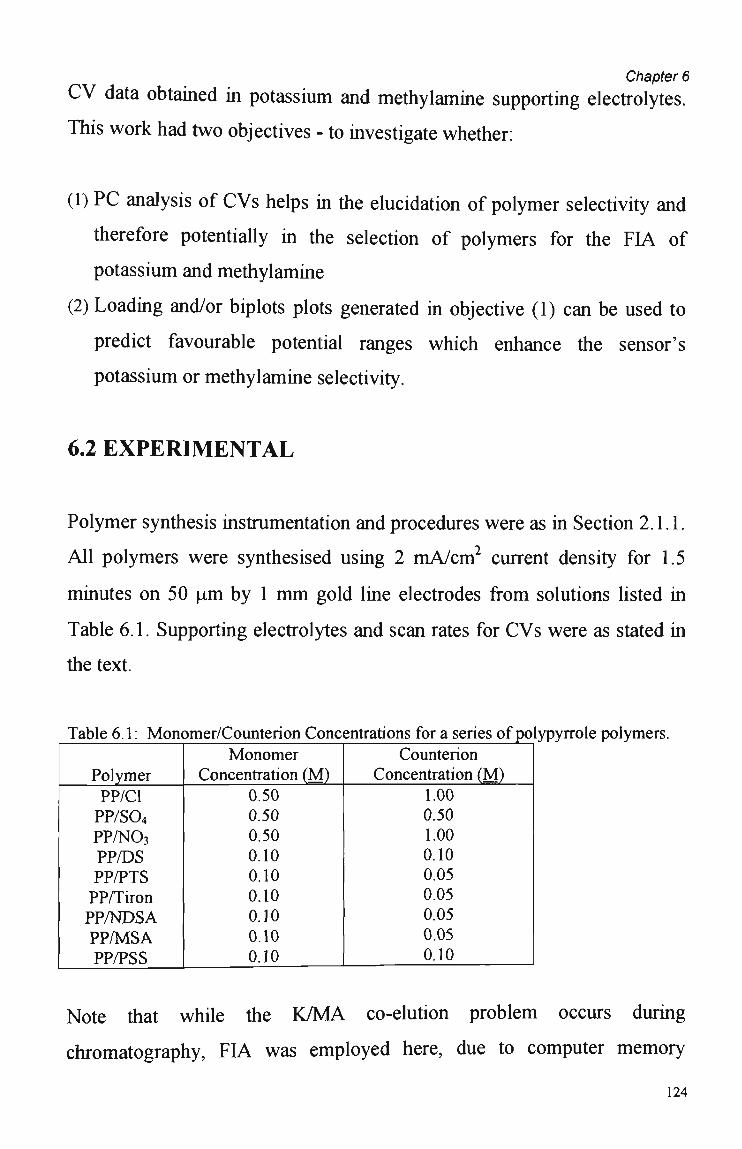
Chapter 6

C V data obtained in potassium and methylamine supporting electrolytes.

This work had two objectives - to investigate whether:

(1) PC analysis of CVs helps in the elucidation of polymer selectivity and

therefore potentially in the selection of polymers for the FIA of

potassium and methylamine

(2) Loading and/or biplots plots generated in objective (1) can be used to

predict favourable potential ranges which enhance the sensor's

potassium or methylamine selectivity.

6.2 EXPERIMENTAL

Polymer synthesis instrumentation and procedures were as in Section 2.1.1.

Ali polymers were synthesised using 2 mA/cm 2 current density for 1.5

minutes on 50 u m by 1 m m gold line electrodes from solutions listed in

Table 6.1. Supporting electrolytes and scan rates for C V s were as stated in

the text.

Table 6.1: Monomer/Counterion Concentrations for a series of po

Polymer PP/Cl PP/S04

PP/NO3 PP/DS PP/PTS PP/Tiron PP/NDSA PP/MSA PP/PSS

Monomer Concentration (M)

0.50 0.50 0.50 0.10 0.10 0.10 0.10 0.10 0.10

Counterion Concentration (M)

1.00 0.50 1.00 0.10 0.05 0.05 0.05 0.05 0.10

ypyrrole polymers.

Note that while the K / M A co-elution problem occurs during

chromatography, FIA was employed here, due to computer memory

124

Chapter 6

constraints. That is, analysis time had to be kept to a minimum. However,

chromatography conditions (operating pressure, suppression of eluent, etc)

were maintained. FIA conditions were as for Section 2.2.1, using

süppressed 20 m M HCI eluent (background conductivity after suppression

was less than 4 uS). Analyte concentrations were as stated in the text.

Chemometric procedures were as for Section 2.4. Data pretreatment

comprised of double centreing and autoscaling in each case.

6.3: RESULTS AND DISCUSSION

6.3.1 OPTIMISATION OF FLOW INJECTION ANALYSIS

D E T E C T I O N P A R A M E T E R S

6.3.1.1 Raw FIA Data

Ordinarily, with pulsed amperometric detection the raw FIA data is

processed so that the response obtained with one current sample point may

be extracted from the rest (Section 2.3.2.1, Figure 2.14). In this way, data

from various current sample points may be used to build up a picture of a

polymer's kinetic behaviour. This was demonstrated with the FIA data in

Chapter 5 (Section 5.3.3). However, an alternative to the current sample

point extraction method would be to leave the whole pulsed current

response intact (in effect using ali current sample points simultaneously).

This would have the advantage of allowing the selection of specific

portions of the peak, rather than one current sample point over ali portions

of the peak. Also, because the data processing is simpler, it is less time

consuming.

125

Chapter 6

For example, the raw data from the FIA of potassium and methylamine

using a pulsed potential waveform (including ali current sample points) is

shown in Figure 6. IA.

< 3 C

g

PP/PSS in K

PP/PSS in MA

time (seconds)

Figure 6.1 A: The total pulsed amperometric response of PP/PSS for the FIA of 10 ppm potassium and 10 ppm methylamine where E, = -0.75 V and E2 = -0.25 V.

008 •

o.oe -

0.04 -

0.02 -

•002 •

•004 •

-006 •

-008 •

-01 -

•0.12 •

0 2 0 4 \ \ 0 6 0.8 1

Time (seconds)

0.25 •

0.2 •

0.15 •

01 •

0 05 •

o •

-005 •

-01 •

-015 •

-02 •

0.2 0.4 Vi 0.6 0 8

Time (seconds)

1

B C Figure 6.1B and C: Comparison of the first and fifth pulses from Figure 6.1 A, of PP/PSS for the FIA of 10 ppm potassium and 10 ppm methylamine where Ei = -0.75 V and E2 = -0.25 V.

Comparison of the potassium and methylamine current curves for this

polymer reveals that in this case, sampling current from the middle of the 126

Chapter 6

pulse (regardless of the current sample point) will probably not yield much

selective information. The most difference between potassium and

methylamine responses occurred over the first few pulses of the peak.

Figures 6.1B and 6.1 C highlight this fact, as they compare the first and the

fifth pulses directly. This clearly demonstrates that the selection of whole

specific pulses rather than current sample points enables the most selective

information to be used.

6.3.1.2 Optimisation of Pulse Detection Parameters

A FIA current sample rate of 100 points/second was used throughout

(reduced to 50 points/second by post-acquisition data processing). Five

pulsed potential waveforms, distributed between the upper and lower C V

potential limits were selected, each with a range of 500 m V (Figure 6.2,

Table 6.2).

C D E

L -0.95

B

0.0 J 0.5

E(Volts)

Figure 6.2: Five potential waveforms used in the pulsed amperometric FIA of potassium and methylamine. A= -0.95 V to -0.45 V, B = -0.75 V to -0.25 V, C = -0.55 V to -0.05 V, D= -0.30 V to 0.20 V, E = 0.00 V to 0.50 V.

Table 6.2: Pulsed potential waveforms used in the FIA of potassium and methylamine.

Waveform* A B C D E

Ei(V) -0.95 -0.75 -0.55 -0.20 0.00

E2(V) -0.45 -0.25 -0.05 0.30 0.50

* Pulse Period = 1 second.

127

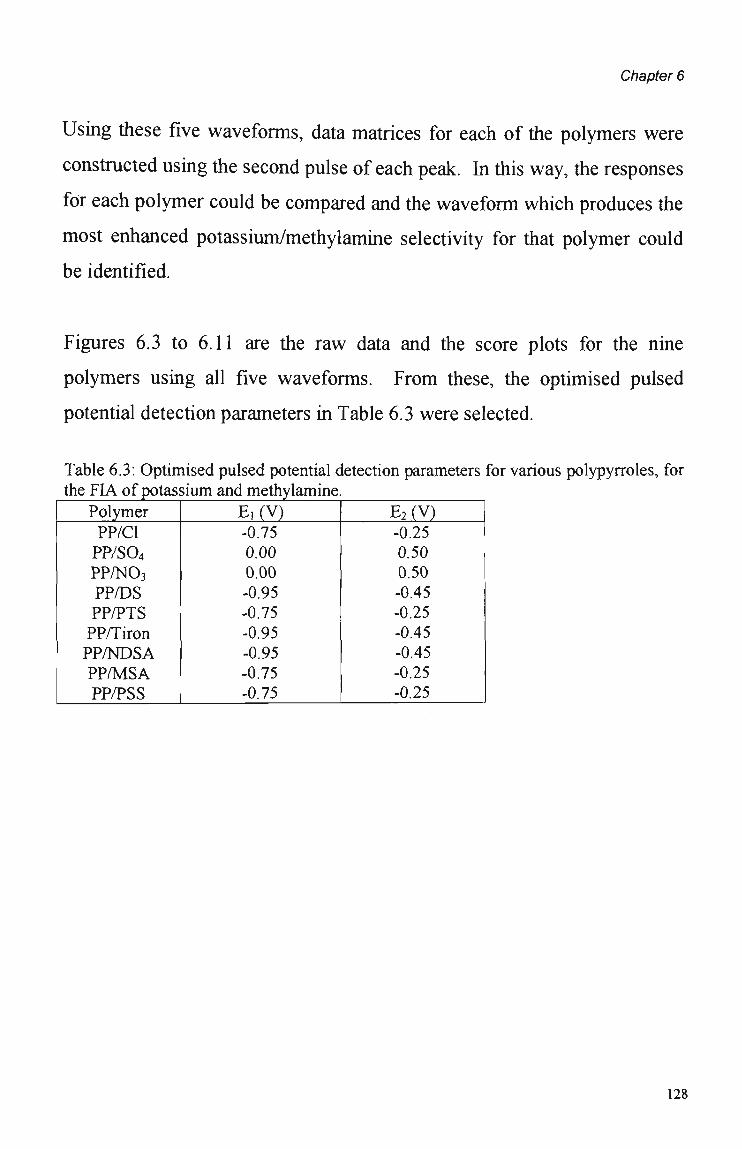
Chapter 6

Using these five waveforms, data matrices for each of the polymers were

constructed using the second pulse of each peak. In this way, the responses

for each polymer could be compared and the waveform which produces the

most enhanced potassium/methylamine selectivity for that polymer could

be identifíed.

Figures 6.3 to 6.11 are the raw data and the score plots for the nine

polymers using ali five waveforms. From these, the optimised pulsed

potential detection parameters in Table 6.3 were selected.

Table 6.3: Optimised pulsed potential detection parameters for various polypyrroles, for the FIA of potassium and methylamine.

Polymer PP/Cl

PP/SO4 PP/NO3 PP/DS PP/PTS PP/Tiron PP/NDSA PP/MSA PP/PSS

E,(V) -0.75 0.00 0.00 -0.95 -0.75 -0.95 -0.95 -0.75 -0.75

E2(V) -0.25 0.50 0.50 -0.45 -0.25 -0.45 -0.45 -0.25 -0.25

128

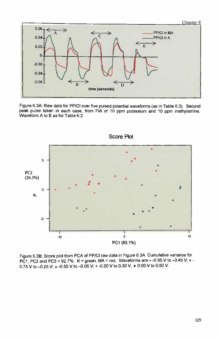
Chapter 6 0.06-r

PP/CI in MA PP/Cl in K

time (seconds)

Figure 6.3A: Raw data for PP/Cl over five pulsed potential waveforms (as in Table 6.3). Second peak pulse taken in each case, from FIA of 10 ppm potassium and 10 ppm methylamine. Waveform A to E as for Table 6.2.

Score Plot

5 -

PC2 (26.3%)

0 -

-5 -

PC1 (63.1%)

Figure 6.3B: Score plot from PCA of PP/Cl raw data in Figure 6.3A. Cumulative variance for PC1, PC2 and PC3 = 92.7%. K = green, M A = red. Waveforms are:+ -0.95 V to -0.45 V; • -0.75 V to -0.25 V; o -0.55 V to -O.05 V; * -0.20 V to 0.30 V; • 0.00 V to 0.50 V.

129

Chapter 6

»T< ; > PP/S04 in MA

PP/S04 in K

time (seconds)

Figure 6.4A: Raw data for PP/S04 over five pulsed potential waveforms (as in Table 6.3). Second peak pulse taken ín each case, from FIA of 10 ppm potassium and 10 ppm methylamine. Waveforms A to E as for Table 6.2.

Score Plot

PC2 (21.7%)

PC1 (60.6%)

Figure 6.4B: Score plot from PCA of PP/SO4 raw data in Figure 6.4A. Cumulative variance for PC1, PC2 and PC3 = 88.8%. K = green, M A = red. Waveforms are:+ -0.95 V to -0.45 V; • -0.75 V to -0.25 V- o -0.55 V to -0.05 V; * -0.20 V to 0.30 V; • 0.00 V to 0.50 V.

130

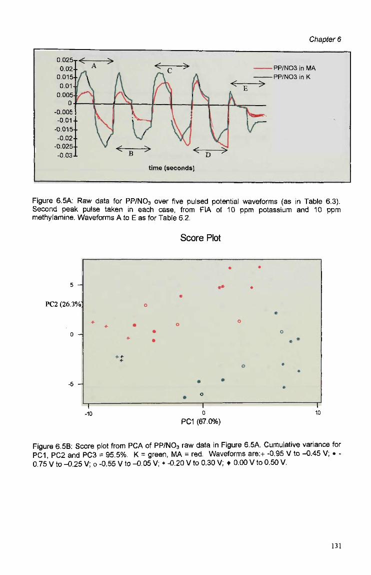
Chapter 6

PP/N03 in MA PP/N03 in K

time (seconds)

Figure 6.5A: Raw data for PP/N03 over five pulsed potential waveforms (as in Table 6.3). Second peak pulse taken in each case, from FIA of 10 ppm potassium and 10 ppm methylamine. Waveforms A to E as for Table 6.2.

Score Plot

5 -

PC2 (26.3%

0 -

-5 -

PC1 (67.0%)

Figure 6.5B: Score plot from PCA of PP/NO3 raw data in Figure 6.5A Cumulative variance for PC1, PC2 and PC3 = 95.5%. K = green, M A = red. Waveforms are:+ -0.95 V to -0.45 V; • -0.75 V to -0.25 V; o -0.55 V to -0.05 V; * -0.20 V to 0.30 V; • 0.00 V to 0.50 V.

131

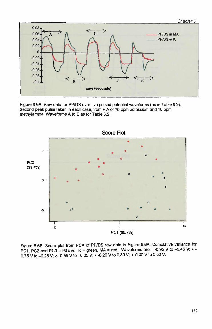
Chapter 6

. PP/DS in MA

.PP/DS inK

time (seconds)

Figure 6.6A: Raw data for PP/DS over five pulsed potential waveforms (as in Table 6.3). Second peak pulse taken in each case, from FIA of 10 ppm potassium and 10 ppm methylamine. Waveforms A to E as for Table 6.2.

Score Plot

5 -

PC2 (28.4%)

0 -

PC1 (60.7%)

Figure 6.6B: Score plot from PCA of PP/DS raw data in Figure 6.6A. Cumulative variance for PC1 PC2 and PC3 = 93.5%. K = green, M A = red. Waveforms are:+ -0.95 V to -0.45 V; • -0.75 V to -0.25 V; o -0.55 V to -0.05 V; * -0.20 V to 0.30 V; • 0.00 V to 0.50 V.

132

Chapter 6

PP/ PTS in MA PP/PTS in K

time (seconds)

Figure 6.7A: Raw data for PP/PTS over five pulsed potential waveforms (as in Table 6.3). Second peak pulse taken in each case, from FIA of 10 ppm potassium and 10 ppm methylamine. Waveforms A to E are as for Table 6.2.

Score Plot

PC2 (21.2%)

PC1 (67.5%)

Figure 6.7B: Score plot from PCA of PP/PTS raw data in Figure 6.7A. Cumulativo variance for PC1, PC2 and PC3 = 92.6%. K = green, M A = red. Waveforms are:+ -0.95 V to -0.45 V; • -0.75Vto-0.25V; o -0.55 Vto-0.05 V; * -0.20Vto 0.30V; • 0.00 Vto 0.50V.

133

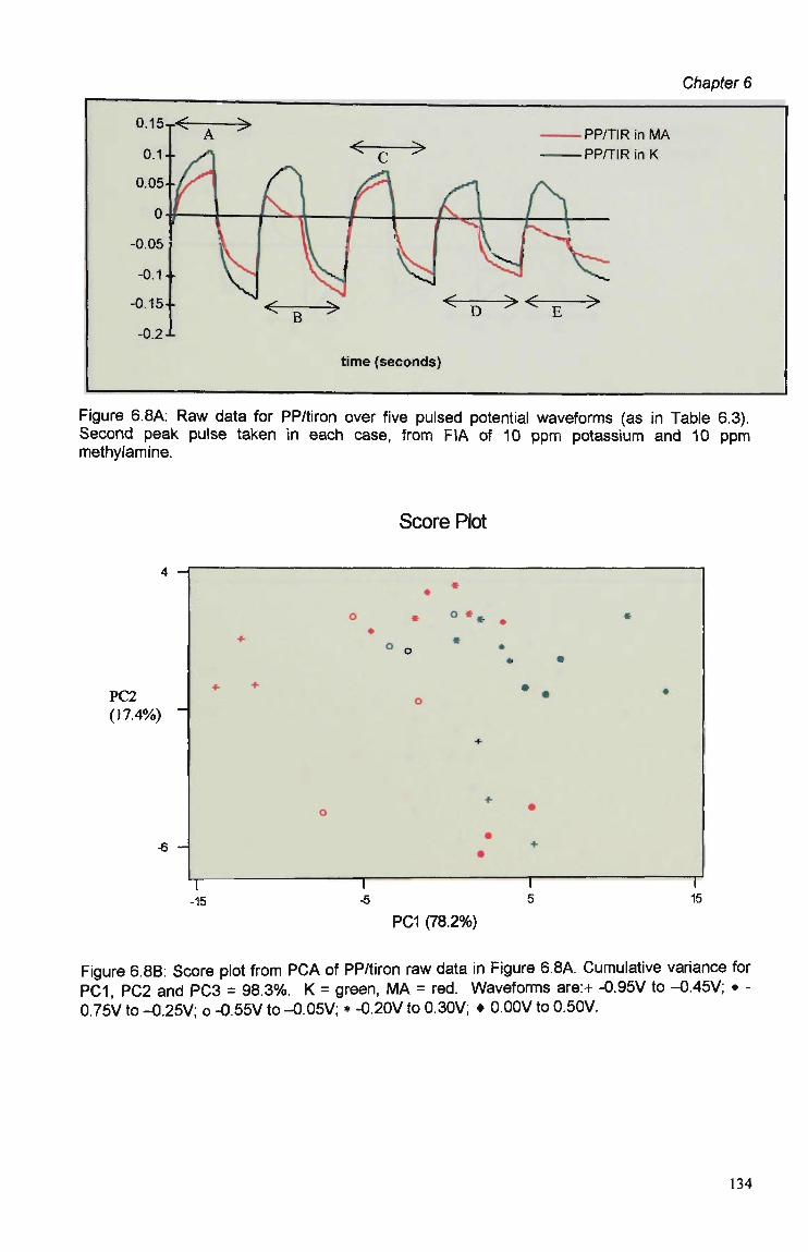
Chapter 6

PP/TIR in MA PP/TIR in K

time (seconds)

Figure 6.8A: Raw data for PP/tiron over five pulsed potential waveforms (as in Table 6.3). Second peak pulse taken in each case, from FIA of 10 ppm potassium and 10 ppm methylamine.

Score Plot

4 -I

PC2 (17.4%)

-15 -5 5

PC1 (78.2%)

Figure 6.8B: Score plot from PCA of PP/tiron raw data in Figure 6.8A. Cumulative variance for PC1, PC2 and PC3 = 98.3%. K = green, M A = red. Waveforms are:+ -0.95V to -0.45V; • -0.75V to -0.25V; o -0.55V to -0.05V; * -0.20V to 0.30V; • 0.00V to 0.50V.

134

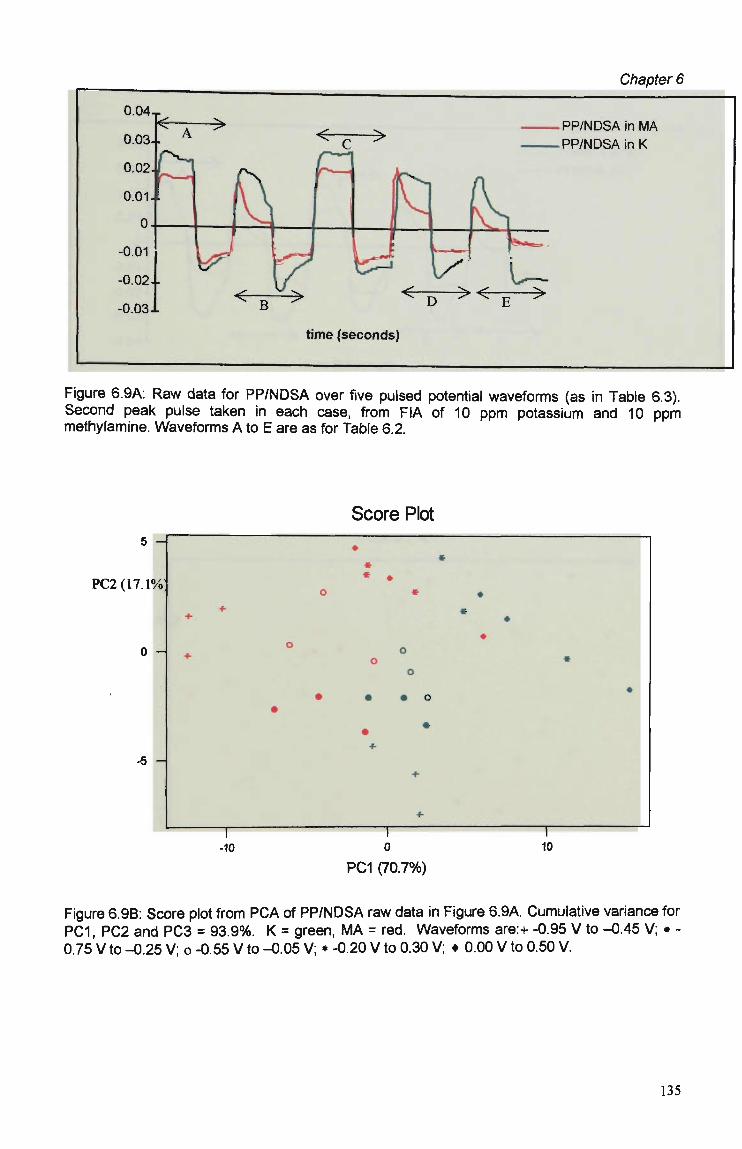
Chapter 6

.PP/NDSAinMA -PP/NDSAinK

time (seconds)

Figure 6.9A: Raw data for PP/NDSA over five pulsed potential waveforms (as in Table 6.3). Second peak pulse taken in each case, from FIA of 10 ppm potassium and 10 ppm methylamine. Waveforms A to E are as for Table 6.2.

Score Plot

PC2(17.l<

-6 -

PC1 (70.7%)

Figure 6.9B: Score plot from PCA of PP/NDSA raw data in Figure 6.9A. Cumulativo variance for PC1, PC2 and PC3 = 93.9%. K = green, M A = red. Waveforms are:+ -0.95 V to -0.45 V; • -0.75 V to -0.25 V; o -0.55 V to -0.05 V; * -0.20 V to 0.30 V; • 0.00 V to 0.50 V.

135

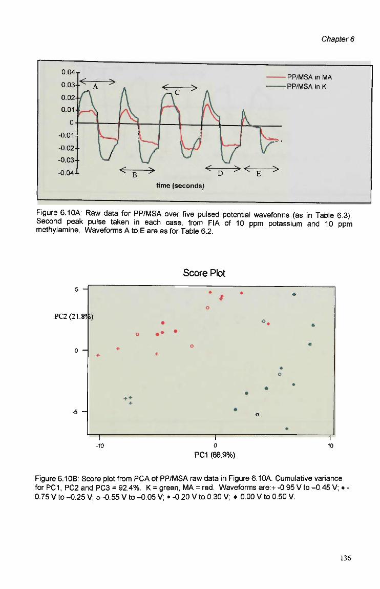
Chapter 6

PP/MSA in MA PP/MSA in K

time (seconds)

Figure 6.10A: Raw data for PP/MSA over five pulsed potential waveforms (as in Table 6.3). Second peak pulse taken in each case, from FIA of 10 ppm potassium and 10 ppm methylamine. Waveforms A to E are as for Table 6.2.

Score Plot

PC2 (21

PC1 (66.9%)

Figure 6.10B: Score plot from PCA of PP/MSA raw data in Figure 6.10A. Cumulativo variance for PC1, PC2 and PC3 = 92.4%. K = green, M A = red. Waveforms are:+ -0.95 V to -0.45 V; • 0.75 V to -0.25 V; o -0.55 V to -0.05 V; * -0.20 V to 0.30 V; • 0.00 V to 0.50 V.

136

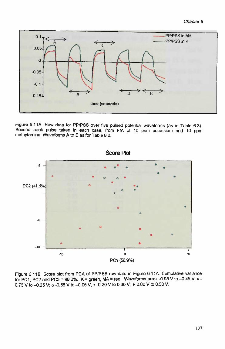
Chapter 6

0.1 _

0.05..

time (seconds)

PP/PSS in MA PP/PSS in K

< D > C E >

Figure 6.11A: Raw data for PP/PSS over five pulsed potential waveforms (as in Table 6.3). Second peak pulse taken in each case, from FIA of 10 ppm potassium and 10 ppm methylamine. Waveforms A to E as for Table 6.2.

Score Plot

5 -

PC2(41.5%;

-5 -

-10 H

PC1 (50.9%)

Figure 6.11B: Score plot from PCA of PP/PSS raw data in Figure 6.11 A. Cumulative variance for PC1, PC2 and PC3 = 98.2%. K = green, MA = red. Waveforms are:+ -0.95 V to -0.45 V; • -0.75 V to -0.25 V; o -0.55 V to -0.05 V; * -0.20 V to 0.30 V; • 0.00 V to 0.50 V.

137

Chapter 6 Using these optimised waveforms, the potassium/methylamine selectivity

of the polymers was improved compared with the selectivity observed

when ali waveforms, or when less selective parameters were used. This is

demonstrated by comparison of score plots generated from P C A using

optimised waveforms (Figure 6.12), ali waveforms together (Figure 6.13)

and a "bad" waveform (Ei = -0.20 V, E 2 = 0.30 V, Figure 6.14). From

Figure 6.12, the five® polymers with optimum potassium/methylamine

selectivity were selected.

In this way the "optimal" chemical and electrochemical detection

parameters for the pulsed amperometric FIA of potassium and

methylamine were determined and are given in Table 6.4.

Table 6.4: Optimised chemical and electrochemical pulsed potential detection parameters for the amperometric FIA of potassium and methylamine.

Polymer PP/Cl PP/DS PP/Tiron PP/MSA PP/PSS

E,(V) -0.75 -0.95 -0.95 -0.75 -0.75

E2(V) -0.25 -0.45 -0.45 -0.25 -0.25

® The use of five polymers equates to a total of about 250 data points, which is desirable for ease of data matrix handling and preprocessing considerations.

138

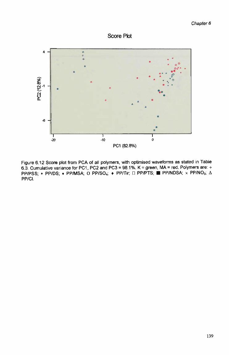
Chapter 6

Score Plot

4 -

CO cvi-1

8 0_

-6 -

PC1 (82.8%)

Figure 6.12 Score plot from PCA of ali polymers, with optimised waveforms as stated in Table 6.3. Cumulative variance for PC1, PC2 and PC3 = 98.1%. K = green, M A = red. Polymers are: + PP/PSS; * PP/DS; • PP/MSA; O PP/S04; • PP/Tir; G PP/PTS; • PP/NDSA; x PP/N03; A PP/Cl.

139

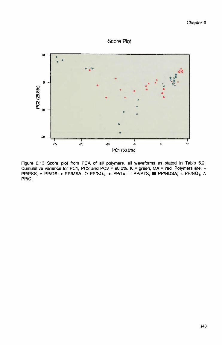
Chapter 6

Score Plot

10 -

00

8 -10 -

-20 -

-15 -5

PC1 (58.6%)

Figure 6.13 Score plot from PCA of ali polymers, ali waveforms as stated in Table 6.2. Cumulative variance for PC1, PC2 and PC3 = 90.0%. K = green, M A = red. Polymers are: + PP/PSS; * PP/DS; • PP/MSA; O PP/S04; • PP/Tir; D PP/PTS; • PP/NDSA; x PP/N03, A PP/Cl.

140

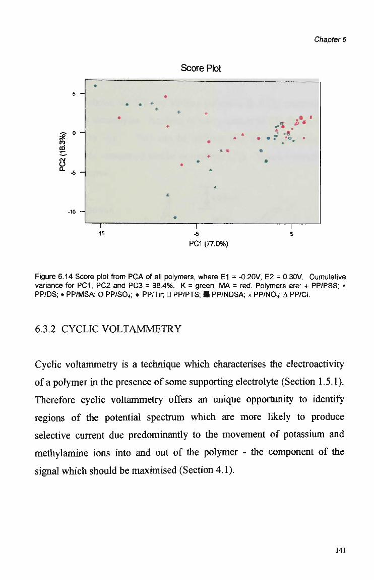
Chapter 6

5 -

CO CO

8

o -

-5 -

-10 -

-15

Score Plot

C • . 'O •

PC1 (77.0%)

Figure 6.14 Score plot from PCA of ali polymers, where E1 = -0.20V, E2 = 0.30V. Cumulative variance for PC1, PC2 and PC3 = 98.4%. K = green, M A = red. Polymers are: + PP/PSS; * PP/DS; • PP/MSA; O PP/S04; • PP/Tir; D PP/PTS; • PP/NDSA; x PP/N03; A PP/Cl.

6.3.2 C Y C L I C V O L T A M M E T R Y

Cyclic voltammetry is a technique which characterises the electroactivity

of a polymer in the presence of some supporting electrolyte (Section 1.5.1).

Therefore cyclic voltammetry offers an unique opportunity to identify

regions of the potential spectrum which are more likely to produce

selective current due predominantly to the movement of potassium and

methylamine ions into and out of the polymer - the component of the

signal which should be maximised (Section 4.1).

141

Chapter 6

6.3.2.1 Visual Analysis of C V s

Figure 6.15 shows the C V s of various polymers in 0.1M potassium and

methylamine electrolytes. Analysis or interpretation of C V data is usually

performed "by eye". This can be difficult and time consuming when

simultaneously comparing similar or multiple CVs. Visual inspection can

also be subjective.

I — i — • — i — ' — r •0.95 -0.4 0.0 0.45

E(Volts)

I 1 • 1 ' 1 • 1 • 0.95 -0.4 0.0 0.45

E(Volts)

| 1 " 1 ' 1 • 1 | 1 • 1 ' 1 ' I -0.95 -0.4 0.0 0.45 -0.95 -0.4 0.0 0.45

E(Volts) E(Volts)

| 1 • 1 • 1 • 1 I 1 ' I ' I , _

• 0.95 -0.4 0.0 0.45 -0.95 -0.4 0.0 0.45

E(Volts) E(Volts)

142

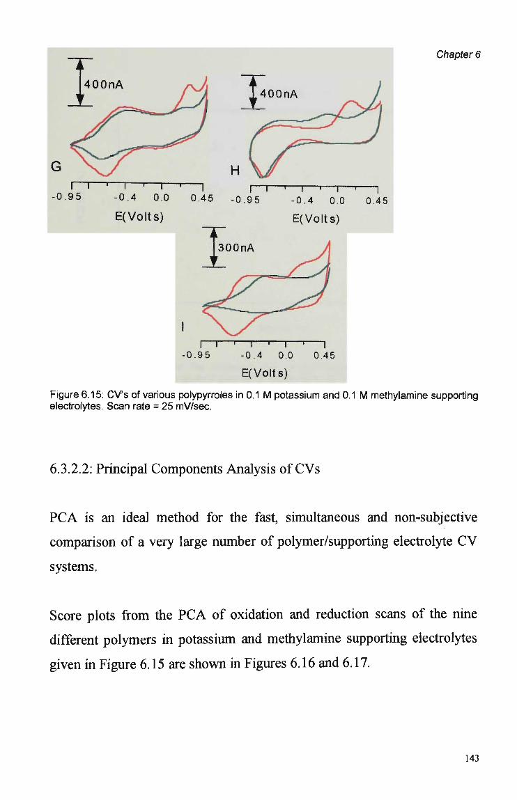
Chapter 6

I r •0.95 -0.4 0.0 0.45 -0.95

E(Volts)

"" 1 • 1 • 1 -0.4 0.0 0.45

E(Volts)

l—r •0.95

"i 1 P 1 ' I •0.4 0.0 0.45

E(Volts)

Figure 6.15: CVs of various polypyrroles in 0.1 M potassium and 0.1 M methylamine supporting electrolytes. Scan rate = 25 mV/sec.

6.3.2.2: Principal Components Analysis of C V s

PCA is an ideal method for the fast, simultaneous and non-subjective

comparison of a very large number of polymer/supporting electrolyte C V

systems.

Score plots from the P C A of oxidation and reduction scans of the nine

different polymers in potassium and methylamine supporting electrolytes

given in Figure 6.15 are shown in Figures 6.16 and 6.17.

143

Chapter 6

Score Plot

10 -

co

a o CL

-10 -

PC1 (43.7%)

Figure 6.16: Score plot for the oxidation scan of the polymers shown in Figure 6.15. Experimental conditions are as for Figure 6.15. Cumulative variance for PC1, PC2 and PC3 = 82.5%. K = green, M A = red. Polymers are: + PP/PSS; * PP/DS; • PP/MSA; O PP/S04; • PP/Tir; D PP/PTS; I PP/NDSA; x PP/N03; A PP/Cl.

144

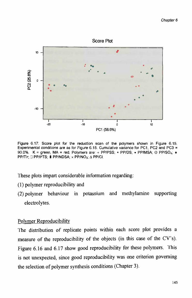
Chapter 6

Score Plot

CD *

+

-20 -10 0 10

PC1 (58.6%)

Figure 6.17: Score plot for the reduction scan of the polymers shown in Figure 6.15. Experimental conditions are as for Figure 6.15. Cumulative variance for PC1, PC2 and PC3 = 90.0%. K = green, M A = red. Polymers are: + PP/PSS; * PP/DS; • PP/MSA; O PP/S04; • PP/Tir; D PP/PTS; I PP/NDSA; x PP/N03; A PP/Cl.

These plots impart considerable information regarding:

(1) polymer reproducibility and

(2) polymer behaviour in potassium and methylamine supporting

electrolytes.

Polymer Reproducibility

The distribution of replicate points within each score plot provides a

measure of the reproducibility of the objects (in this case of the C V s ) .

Figure 6.16 and 6.17 show good reproducibility for these polymers. This

is not unexpected, since good reproducibility was one criterion governing

the selection of polymer synthesis conditions (Chapter 3).

145

Chapter 6

Polymer Behaviour in Potassium and Methylamine

The position of each object on the plot is indicative of how similar or

dissimilar it is to other objects. The C V s of some polymers in potassium

and methylamine are more alike than others. This would imply that:

(1) some polymers have better potassium/methylamine discrimination

capabilities than others and that

(2) some polymers have similar potassium/methylamine selectivities,

despite having different counterions.

6.3.2.2 The PCA of CVs for the Prediction of Optimal Electrochemical

and Chemical Detection Parameters.

It is not unreasonable to expect that chemometric analysis of CVs might be

useful to indicate polymer selectivity in the flow cell, since the C V

depends upon the ion exchange character of a polymer, as does the

selectivity of a polymer in the flow cell.

The placement of the various CV objects in the score plots suggests that:

(1) the C V s of PP/Tir and PP/PSS are somewhat alike,

(2) PP/PTS, PP/N0 3 and PP/SO4 likewise have similar C V responses and

(3) P P / N D S A and P P / M S A (especially with regards to the variance

accounted for by PCI) may have similar responses.

These observations do find some correlation in the score plots of the FIA

responses in Section 6.3.1.2. In particular, the score plot in Figure 6.13

(which takes into account the responses of the polymers over ali

waveforms, and therefore over the whole potential spectrum) shows that

the above polymer C V groupings also apply to the polymer FIA responses.

146

Chapter 6

This could translate into an ability to predict which polymers might exhibit

similar or dissimilar selectivities in the flow cell without the time

consuming and more experimentally complex task of screening their

responses in the flow cell over numerous potential ranges.

The loading and biplots from the PCA of the CV data elucidate the

importance of each of the potentials (the variables) to the various C V s (the

objects). B y using these plots generated by the P C A of C V oxidation and

reduction data (Figures 6.18 and 6.19), the potentials with the greatest

importance to the C V s were identifíed and are listed in Table 6.5.

These values appear to favour the negative potential ranges, most being

less than -0.05 V. This would suggest that "optimum" waveforms

(waveforms which would enhance potassium/methylamine selectivity more

than others) would be those which cover the more negative potential

ranges.

This was found to be the case, with optimal waveforms for most of the

polymers being over the -0.95 V to -0.25 V potential range (Table 6.3).

The other polymers (PP/N03 and PP/SO4, whose optimum waveforms were

over the positive potential range) had poor potassium/methylamine

discrimination capabilities in any case, regardless of which waveform was

used.

147

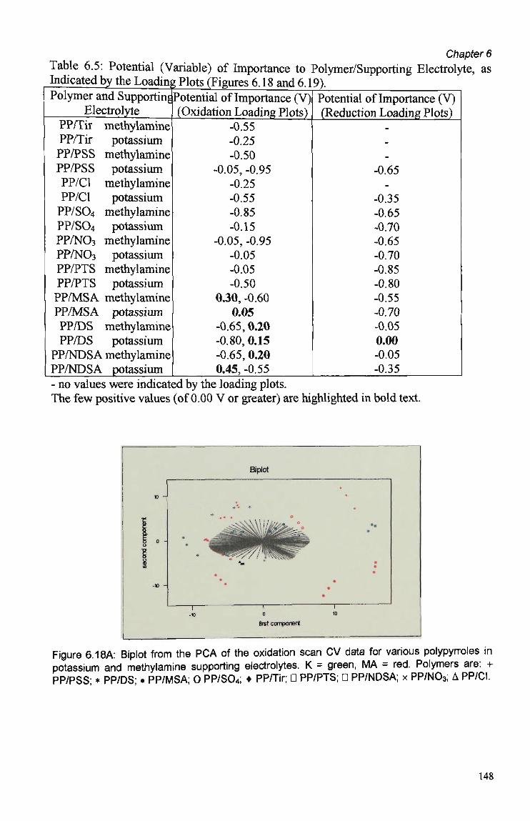
Chapter 6 Table 6.5: Potential (Variable) of Importance to Polymer/Supporting Electrolyte, as Indicated by the Loading Plots (Figures 6.18 and 6.19). Polymer and Supporting

Electrolyte PP/Tk methylamine PP/Tir potassium PP/PSS methylamine PP/PSS potassium PP/Cl methylamine PP/Cl potassium PP/SO4 methylamine PP/SO4 potassium PP/NO3 methylamine PP/NO3 potassium PP/PTS methylamine PP/PTS potassium PP/MSA methylamine PP/MSA potassium PP/DS methylamine PP/DS potassium

PP/NDSA methylamine PP/NDSA potassium

Potential of Importance (V) (Oxidation Loading Plots)

-0.55 -0.25 -0.50

-0.05, -0.95 -0.25 -0.55 -0.85 -0.15

-0.05, -0.95 -0.05 -0.05 -0.50

0.30, -0.60 0.05

-0.65,0.20 -0.80, 0.15 -0.65,0.20 0.45, -0.55

Potential of Importance (V) (Reduction Loading Plots)

_

_

.

-0.65 -

-0.35 -0.65 -0.70 -0.65 -0.70 -0.85 -0.80 -0.55 -0.70 -0.05 0.00 -0.05 -0.35

- no values were indicated by the loading plots. The few positive values (of 0.00 V or greater) are highlighted in bold text.

10 -

second com

0 1

-10 -

Biplot

/v +

"• . . . 0

^ÊÊÈÈÈ^ÈIÊ^^

« » «

1 1 -10 0

lirst component

,

« • *

10

,

*

« *

Figure 6.18A: Biplot from the PCA of the oxidation scan CV data for various polypyrroles in potassium and methylamine supporting electrolytes. K = green, MA = red. Polymers are: + PP/PSS; * PP/DS; • PP/MSA; O PP/S04; • PP/Tir; 0 PP/PTS; D PP/NDSA; x PP/NO3, A PP/CI.

148

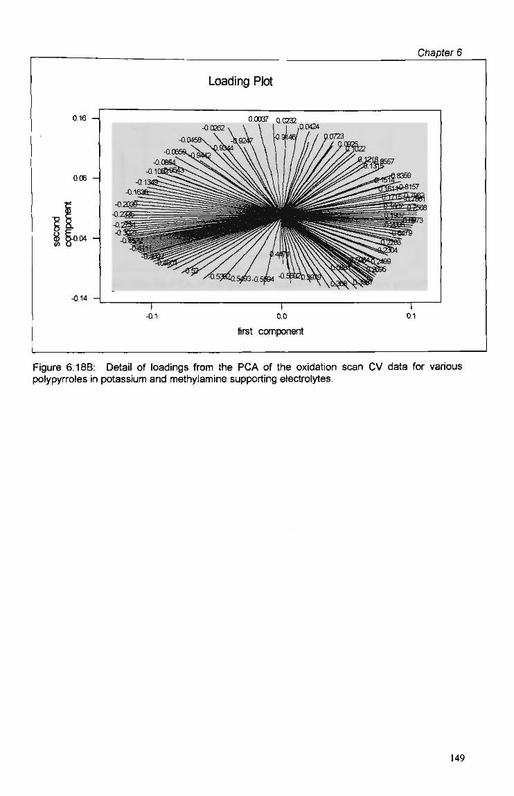
Chapter 6

Loading Plot

0.16 -

0.06 -

8 &0.04 -U) o

-0.14 -

-0.0262 0.0037 Q.0232

,0.0424

-0.1 0.0

first component

0.1

Figure 6.18B: Detail of loadings from the P C A of the oxidation scan C V data for various polypyrroles in potassium and methylamine supporting electrolytes.

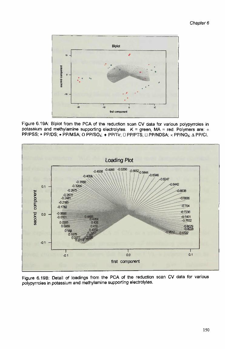
Chapter 6

10 -

I s ° _

I -10 -

• •

1 -20

Biplot

/

• Qfc- •

* *

* • •

• i i i -10 0 10

jrst component

Figure 6.19A. Biplot from the P C A of the reduction scan C V data for various polypyrroles in potassium and methylamine supporting electrolytes. K = green, M A = red. Polymers are: + PP/PSS; * PP/DS; • PP/MSA; O PP/S04; • PP/Tir; D PP/PTS; D PP/NDSA; x PP/N03; A PP/Cl.

0.1

0.0

8

-0.1

Loading Plot

<MW*«? .ff? fSRB-0. 5844

-0.8029 -0.8228

-0.1 0.0

first component

0.1

Figure 6.19B: Detail of loadings from the P C A of the reduction scan C V data for various polypyrroles in potassium and methylamine supporting electrolytes.

150

Chapter 6

6.4 SUMMARY AND CONCLUSIONS

PCA was performed on both FIA and CV data with the aim of identifying

those chemical and electrochemical pulsed amperometric detection

parameters which enhance potassium and methylamine selectivity.

The strategy of representing kinetic selectivity by a single, but whole pulse

was adopted when it was observed that in the case of potassium and

methylamine, only the initial portion of the peak exhibited any difference

in response between those two analytes.

As expected, the response depended upon polymer composition and pulsed

potential parameters. With the aid of PCA, the most favourable chemical

and electrochemical detection parameters for each polymer were identifíed,

and for the five "best" polymers were: -0.75 V to -0.25 V for PP/Cl,

P P / M S A and PP/PSS, and -0.95 V to -0.45 V for PP/DS and PP/Tiron. A n

improvement in potassium/methylamine selectivity when these "tuned"

parameters were employed, was observed.

The exploration of the use of PCA of CVs as a much faster and simpler

way of identifying optimum parameters, or of eliminating poorer ones,

proved effective. It was shown that based on CVs, a judgement can be

made on the potential range likely to give enhanced

potassium/methylamine selectivity for a polymer. PP/Cl showed

particularly good agreement between the predicted optimal potential range

(found using C V data) and the actual optimal range found by P C A of FIA

data. Even in cases where the optimal potential range could not be

specifically chosen, P C A of the C V s did limit the choice considerably.

151

Chapter 6

This work effectively demonstrated polymer tuning in practise and

introduced the use of P C A using C V data to predict the polymers and

waveforms most likely to exhibit enhanced potassium/methylamine

selectivity. This procedure can be adapted for any polymer/analyte

combination that is desired and may therefore provide a much more rapid

(and experimentally simpler) way of screening polymers and

electrochemical conditions for target analyte(s).

152

Chapter 7

CHAPTER 7

THE ANALYSIS OF POTASSIUM AND

METHYLAMINE MIXTURES USING THE

CONDUCTING ELECTROACTIVE POLYMER-

BASED SENSING SYSTEM

7.1 INTRODUCTION

The ability to "tune" the selectivities of CEP sensors was demonstrated for

potassium and methylamine in Chapter 6. The application of the "tuned"

sensing system to the problem of potassium and methylamine peak purity

in FIA is the subject of this Chapter.

Partial Least Squares Regression (PLS, Section 1.7.3) may be used to

model the relationship between peak purity and the responses of the

optimised sensors. This strategy would then allow the quantification of

"unknown" responses (the test set), based on the behaviour of known

responses (the training set).

7.2 EXPERIMENTAL

Polymer preparation procedures were as for Section 6.2. Polymers and

pulsed potential waveforms were as for Table 7.1.

Conditions and instrumentation for FIA of potassium and methylamine

mixtures were as given in Table 2.2 (suppressed eluent, flow rate,

operating pressure, etc). 153

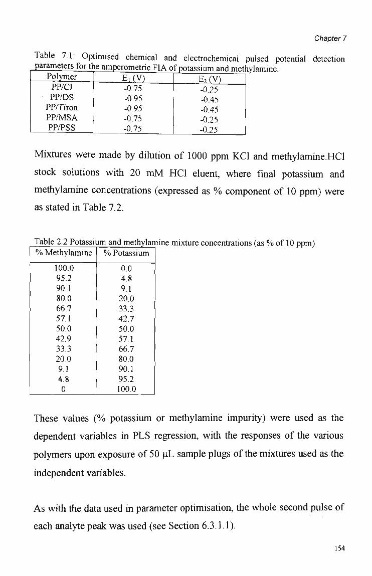
Chapter 7

Table 7.1: Optimised chemical and electrochemical pulsed potential detection parameters for the amperometric FIA of potassium and methylamine.

Polymer PP/Cl PP/DS

PP/Tiron PP/MSA PP/PSS

Ei(V) -0.75 -0.95 -0.95 -0.75 -0.75

E2(V) -0.25 -0.45 -0.45 -0.25 -0.25

Mixtures were made by dilution of 1000 ppm KCI and methylamine.HCl

stock solutions with 20 m M HCI eluent, where final potassium and

methylamine concentrations (expressed as % component of 10 ppm) were

as stated in Table 7.2.

Table 2.2 Potassium and methylamine mixture concentrations (as % of 10 ppm) % Methylamine

100.0 95.2 90.1 80.0 66.7 57.1 50.0 42.9 33.3 20.0 9.1 4.8 0

% Potassium

0.0 4.8 9.1 20.0 33.3 42.7 50.0 57.1 66.7 80.0 90.1 95.2 100.0

These values (% potassium or methylamine impurity) were used as the

dependent variables in PLS regression, with the responses of the various

polymers upon exposure of 50 uL sample plugs of the mixtures used as the

independent variables.

As with the data used in parameter optimisation, the whole second pulse of

each analyte peak was used (see Section 6.3.1.1).

154

Chapter 7

Data treatment for P C A and PLS (Section 2.4) consisted of matrix double

centring and autoscaling.

7.3 RESULTS AND DISCUSSION

7.3.1 PRINCIPAL COMPONENTS ANALYSIS (PCA)

Using the polymers and waveforms optimised in Chapter 6, data from the

analysis of various potassium/methylamine mixtures (Table 7.2) was

obtained. Score plots from this analysis showed that the responses do fali

into groups or classes according to peak composition (Figure 7.1).

Figure 7.1 A: Example of raw data (for simplicity, 3 peaks are shown only)

Chapter 7

75

PC2 (25.8 %)

5

-5

-15

o

-20

Score Plot o

o

o

* :

o

*

• • •

--15 -10 -5 0 5 10

PC1(51.7%)

* *

*

15 20 25

Figure 7.1B Score plot from PCA of "optimised" data matrix (sample shown in Figure 7.1A).0 (red) 100% MA; + 95.3% MA;.x 90.1% MA; • 80.0% MA; D 66.7% MA; • 57.1% MA; A 50.0% MA; • 57.1% K; > 66.7% K; V 80.0% K; 0 90.1% K; * 95.3% K; O (green) 100% K.

7.2.2 PARTIAL LEAST SQUARES REGRESSION ANALYSIS (PLS)

PLS regression analysis was performed on this data. Optimum number of

principal components for the model was found to be 18 (see Appendix

7.1). The final PLS model development involved cross-validation using

the "leave one out method" for 18 components. The data was split into

two sets (training and test sets by taking one object from each known

percentage) and the ability to predict the percentage purity of the unknown

set was tested. The results are shown in Figure 7.2 and listed in Table 7.3.

156

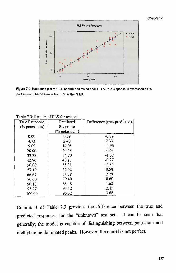
Chapter 7

• = ftted

• = xvsl

Figure 7.2: Response plot for PLS of purê and mixed peaks. The true response is expressed as %

potassium. The difference from 100 is the % MA.

Table 7.3: Results of PLS for test set. True Response (% potassium)

0.00 4.73 9.09 20.00 33.33 42.90 50.00 57.10 66.67 80.00 90.10 95.27 100.00

Predicted Response

(% potassium) 0.79 2.40 14.05 20.63 34.70 43.17 55.31 56.52 64.38 79.40 88.48 93.12 96.32

Difference (true-predicted)

-0.79 2.33 -4.96 -0.63 -1.37 -0.27 -5.31 0.58 2.29 0.60 1.62 2.15 3.68

Column 3 of Table 7.3 provides the difference between the true and

predicted responses for the "unknown" test set. It can be seen that

generally, the model is capable of distinguishing between potassium and

methylamine dominated peaks. However, the model is not perfect.

PLS Fit and PrecSction

T , r 0 50 100

true response

157

Chapter 7

This is almost certainly a consequence of the irreproducibility within the

data. A likely source of error may arise because of one practical difficulty

encountered when using a single pulse out of the whole analyte peak. The

problem is that the waveform and the analyte peak cannot always be

synchronised when the sample is injected manually (as is the case here).

For example, in the extreme case, represented in Figure 7.3, injection 1

begins on the lower potential value, whereas injection 2 begins on the

upper potential value. This happens because the waveform (or the

injection) is "out of phase" by just 500msec. The shaded área of the figure

highlights the difference between the responses obtained for the two peaks

when the "second" pulse is sampled (beginning with the upper potential

value). The responses will apparently be different, not because the

polymers' response is irreproducible, but rather because the analyses are

not synchronised.

The best way to overcome this problem would be to automate the pulsing

and injection procedures so that the two are precisely timed and controlled

together. For this, one computer would have to automate the injector and

the waveform generator.

Alternatively the flow rate could be slowed down, effectively stretching

the peak out over more pulses so that (relatively speaking) the timing of

the pulse becomes less criticai. This is not ideal, however, since this would

make the FIA or chromatography slower.

158

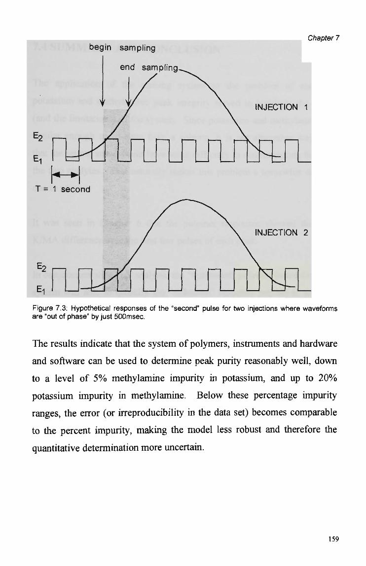
Chapter 7

INJECTION 1

Figure 7.3: Hypothetical responses of the "second" pulse for two injections where waveforms are "out of phase" by just 500msec.

The results indicate that the system of polymers, instruments and hardware

and software can be used to determine peak purity reasonably well, down

to a levei of 5 % methylamine impurity in potassium, and up to 2 0 %

potassium impurity in methylamine. Below these percentage impurity

ranges, the error (or irreproducibility in the data set) becomes comparable

to the percent impurity, making the model less robust and therefore the

quantitative determination more uncertain.

begin sampling

end sampling.

r= 1 second

159

Chapter 7

7.4 SUMMARY AND CONCLUSION

The application of the sensing system to the problem of resolving

potassium and methylamine peak integrity served to highlight the power

(and the limitations) of the system. Since potassium and methylamine are

similar enough to co-elute from a column, it is not altogether surprising

that the sensor array would have some difficulty in discriminating between

the two analytes. This naturally makes this problem a somewhat difficult

one to resolve.

It was seen in Chapter 6 that the polymer responses showed the most

K / M A difference over the first few pulses of each peak.

In conjunction with PLS analysis, the "optimised" polymer-based detection

system was able to quantify the "unknown" response purifies to within a

few percent in most cases. This was despite the irreproducibility that is

inherent when using one pulse over such a small portion of the peak. This

irreproducibility may account for the inability of the system to discriminate

purê peaks from those with low percent impurity in the "unknown" data

set.

Chromatography or FIA systems with pulsed electrochemical detection

instrumentation, which use a "remote" system control option are

commercially available.242 These systems allow the synchronising of

waveforms and injection times. A similar adaptation of the polymer-based

detection system would eliminate a large source of error and improve the

quantitative capabilities of the system.

160

Chapter 7

In any case, the system has been shown to be effective in resolving peak

integrity, certainly to the point where it can discriminate between purê and

very impure potassium peaks, something for which conventional

conductivity detection is useless.

161

Chapter 8

CHAPTER 8

GENERAL CONCLUSIONS AND FUTURE WORK

8.1 GENERAL CONCLUSIONS

The features of natural chemical sensing systems which enable them to

detect, process, identify and record various tastes and odours can be

emulated by appropriate synthetic hardware and software components. In

this work, a generic, synthetic sensing system for ion chromatographic

applications was realised. For this, analytical, electrochemical and

chemometric principies as well as instrument development, electrode array

microfabrication and conducting electroactive polymer technologies were

pooled.

Chemical, electrochemical and kinetic selectivity possibilities of the

sensors were studied by the amperometric detection of a number of

electroinactive anions and cations (Chapter 5). The sensitivity orders of

C E P sensors and conductivity detection confirmed that the polymer

responses are not dominated by the conductivity of the analyte plugs. The

analytical performance of the sensors was found to be dependent on the

detection parameters. Ultimately, the CEP-based sensors did not out-

perform conventional conductivity detection in a sensitivity sense. Rather,

it is the selectivity possibilities which give C E P coated electrodes their

advantage in such applications, justifying their use as the sensing

components of this generic system.

This work also brought to light one of the practical difficulties of using

materiais which have so many selectivities. A way had to be found of 161

Chapter 8

"tuning" the system, or of finding those chemical, electrochemical and

kinetic parameters which would maximise the array's ability to

discriminate between certain analytes.

This was achieved using in two different approaches; by the PC analysis of

(1) FIA and (2) C V response data of polymers to potassium (K) and

methylamine ( M A ) solutions. (K and M A co-elution during cation

chromatography is a known problem and is therefore an ideal "test"

application for the sensing system).

In the first strategy, FIA data comprised of whole pulses instead of

individual current sample points was used as described in Chapter 6. This

effectively enabled ali current sample points (csp) over the most selective

portion of the analyte peak to be used at once - a faster data processing

option than the "csp extraction" method, and more appropriate in this case.

This example of raw data manipulation clearly demonstrates how the data

handling procedures of the multichannel D A Q system are more adaptive

than those of conventional pulsed electrochemical detectors. In this way,

those polymers and waveforms which gave the most different K and M A

responses were identifíed. These were: PP/Cl, PP/MSA, PP/PSS with

switching potentials of -0.75 V and -0.25 V; PP/DS and PP/tir with

switching potentials of-0.95 V and -0.45 V.

The second and unprecedented optimisation method using CV data was

more predictive. The results showed good agreement with the parameters

obtained with the FIA data. At the very least, biplots generated from the

P C A did serve to limit the "optimal" potential range for K / M A selectivity.

162

Chapter 8

This tuning procedure is many times faster than the other, FIA

experimentally intensive screening method.

Finally, the tuned system was applied to the determination of K and MA

peak integrity. P L S analysis of purê and impure peaks allowed the

"unknown" responses to be determined, up to 5 % M A impurity in K, or to

2 0 % K impurity in M A .

It is realised that there are many variables which can effect the outcome of

such regression (and other chemometric) analyses. Such experimental

variables m a y include electrode reproducibility, polymerisation parameters,

chromatographic conditions, voltammetric parameters and the data analysis

approach. It is acknowledged here that the complexity of the analysis

should therefore not be underplayed. However it was for this reason that

only the most reproducible electrodes and polymers were selected.

Similarly, the reproducibility of the electrode response with certain

electrochemical conditions was considered to be just as important as

electrode selectivity in deciding the final composition of the array. In

short, every effort was made to minimise any variability in electrode

response which could be assigned to anything but that due to changes in

peak integrity.

This application served to demonstrate the advantages of the multichannel

potentiostat and data acquisition system which could generate and record

up to eight independem channels of data simultaneously. This contrasts

with other commercial, more conventional FIA or chromatographic

detectors which are typically single channel only. This approach allows the

sampling of discrete parts of the applied potential waveform, which usually

163

Chapter 8

needs to be specified before the analysis. The multichannel D A Q system

together with Labview virtual instrumentation records a continuous stream

of data from each channel at a rate of up to 100 points/sec/channel.

Further, post acquisition processing easily and quickly open up many data

manipulation options not available with commercial detectors. This did

prove advantageous for the chemometric analysis of potassium (K) and

methylamine ( M A ) peaks, as discussed above.

Various conducting polymer materiais were electrochemically coated onto

photolithographically produced Si02/gold microelectrode arrays. The ease

of deposition was found to be dependent upon the nature and concentration

of monomer and counterion, current density as well as electrode size and

shape. The application of nafion pre-coatings was investigated in order to

prevent mass transfer of oligomers away from the electrode surface during

polymer deposition. This was ultimately found to be unnecessary as a

range of polypyrrole were finally deposited on the line microelectrodes.

These were polypyrroles of chloride (PP/Cl), sulphate (PP/S04), nitrate

(PP/NO3), dodecylsulphate (PP/DS), paratoluene sulphonate (PP/PTS),

tiron (PP/tir), naphthalenedisulphonic acid (PP/NDSA), 2-mesitylene

sulphonic acid (PP/MSA), and poly(4-styrenesulphonate) (PP/PSS)

counterions. The optimal growing conditions for these polymers were

found to be 2 mA/cm 2 current density for 2.5 minutes on the 50 jum by 1

m m gold line electrodes.

These sensing elements proved ideal as transducers for pulsed

amperometric detection of electroactive anions and cations after ion

chromatography and FIA. The pulsed waveform allowed controlled ion

exchange throughout the polymer matrix, and therefore the rapid

164

Chapter 8

regeneration of the polymer matrix. Further, the pulsed waveform

permitted the exploration of both electrochemical and kinetic selectivity

options as discussed in Chapter 4.

8.2 FUTURE WORK

This research has highlighted a number of áreas for further investigation.

The low percentage impurity peaks were more difficult to quantify,

probably because of the inherent experimental errors that arise due to the

lack of synchronisation between waveforms and injections for replicate

analyses. The automation of the pulsing and injection procedures has been

identifíed as the best way to eliminate this experimental error.

Another aim for future work would be to improve the sensitivity of the

sensors, without compromising their selectivity. Increasing the amount of

polymer deposited was shown to be a poor strategy as there is a threshold

polymer thickness above which current due to analyte conductivity

dominates the signal. Another possibility involves the lowering of noise

leveis. This is an instrumental consideration and may involve increasing

the electrical shielding of the circuits and connections.

The system could be adapted for any number of applications, since it has

been shown throughout this thesis that the sensors, and even the D A Q may

be manipulated or tuned to suit any analysis. Future workers may wish to

address the possibility of refíning this system to the point where the need

for an ion chromatography set-up is eliminated altogether. This would

represent a considerable development in the pursuit of inexpensive,

portable and adaptive electrochemical sensing systems.

165

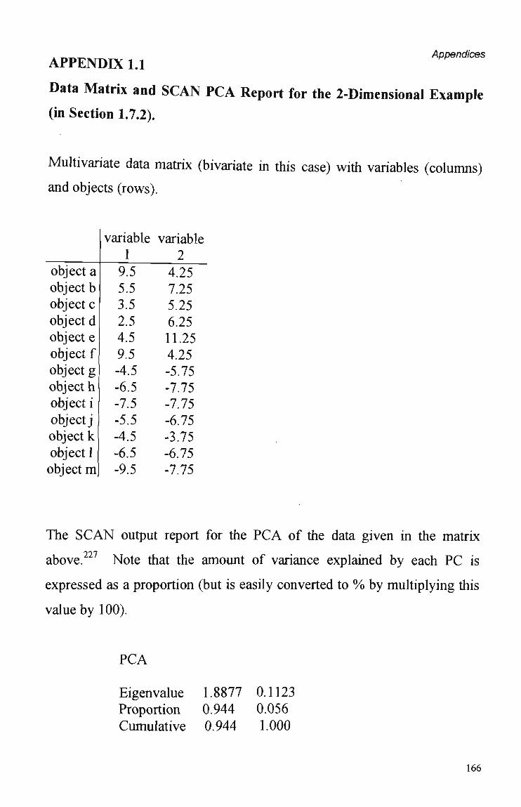
Appendices APPENDIX 1.1

Data Matrix and SCAN PCA Report for the 2-Dimensional Examph

(in Section 1.7.2).

Multivariate data matrix (bivariate in this case) with variables (columns)

and objects (rows).

object a object b object c object d object e object f object g object h object i object j object k object 1 object m

variable variable 1 9.5 5.5 3.5 2.5 4.5 9.5 -4.5 -6.5 -7.5 -5.5 -4.5 -6.5 -9.5

2 4.25 7.25 5.25 6.25 11.25 4.25 -5.75 -7.75 -7.75 -6.75 -3.75 -6.75 -7.75

The S C A N output report for the PCA of the data given in the matrix 227 above. Note that the amount of variance explained by each PC is

expressed as a proportion (but is easily converted to % by multiplying this

value by 100).

PCA

Eigenvalue Proportion Cumulative

1.8877 0.1123 0.944 0.056 0.944 1.000

166

4 Appendices

APPENDIX 2.1 The following equipment was made in the University of Wollongong

Physics Department Electrical Workshop:

nanogalvanostat

faraday cage

waveform generator

167

Appendices

A P P E N D I X 2.2

The Chemical Suppression Of Eluents For Ion-Chromatography243'244

In ion chromatography or HPLC applications, an eluent such as 21 mM

N a O H must be chemically suppressed, so that the background conductivity

is lowered and the analyte signal to eluent background conductivity ratio is

increased.

The suppressor (eg AMMS-II, Dionex) works on a principal of ion

exchange across a membrane which (in the case of the N a O H eluent)

allows the selective exchange of sodium ions with the hydrogen ions of the

regenerant solution (25-50 m N H 2S0 4, Figure 2.1.1). The result is a

suppressed eluent which is essentially water.

The cations of the sample plug are similarly replaced by hydrogen ions. In

the case of the 20 m M HCI eluent, a CMM-II suppressor allows the ion

exchange of the Cl anions with the O H ions of the 100 m N T B A O H . Once

again the resulting suppressed eluent is water.

168

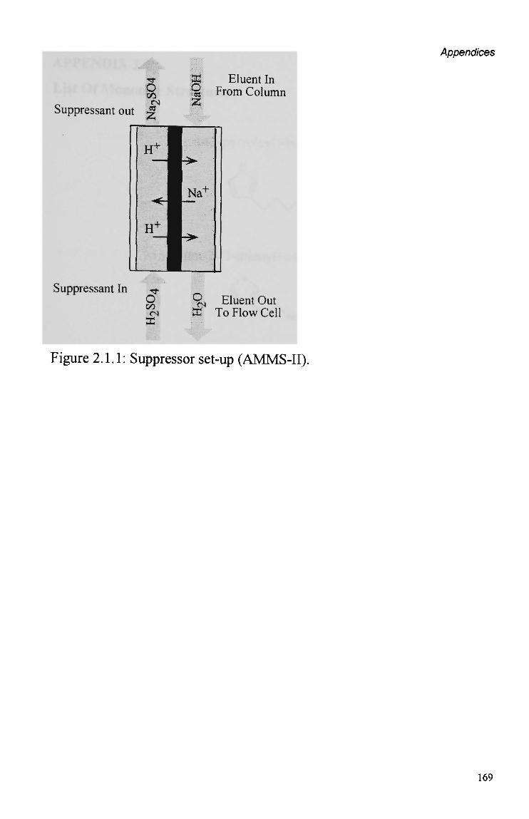
ã f f i Eluent In 9 From Column

Suppressant out jg

Appendices

Suppressant In rj-O O, Eiuen t Qut cs H To Flow Cell

Figure 2.1.1: Suppressor set-up (AMMS-II).

169

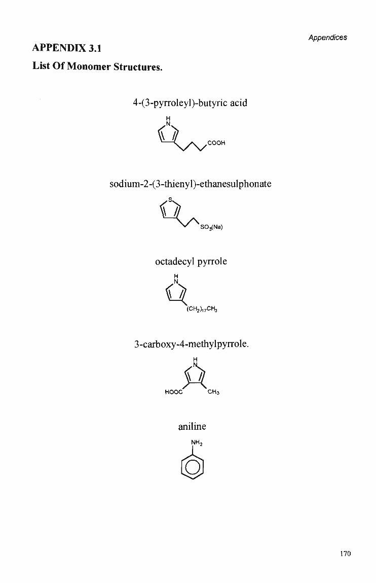
APPENDIX 3.1

List Of Monomer Structures.

4-(3-pyrroleyl)-butyric acid

H

.COOH

sodium-2-(3-thienyl)-ethanesulphonate

^ SOg(Na)

octadecyl pyrrole

H N

O (CHJ^TCH, 3 -carboxy-4-methy lpyrrole.

H

A HOOC CH3

aniline

NH2

APPENDIX 3.2

List of Counterion Structures

Tiron 2-mesitylene sulphonic acid 4-sulphobenzoic acid

Appendices

CH,

HO 'SOaíNa)

OH

H3C

COOH

CH,

S04CI n

so.

p- toluene sulphonate 4-ethylbenzensulphonic acid 1,3-benzene disulphonic acid

ÇH3 CH2CH3

O O O'"" SO, SO3- SOgCNa)

4-hydroxybenzenesulphonic acid

benzene sulphonic acid dodecylsulphate

OH

O O SO^Na) SO^Na) S03Na

chromazurol-s eriochromcyanine R C

NaOO

CH3

S03Na

HO T

S03Na

N<^

C H 3

171

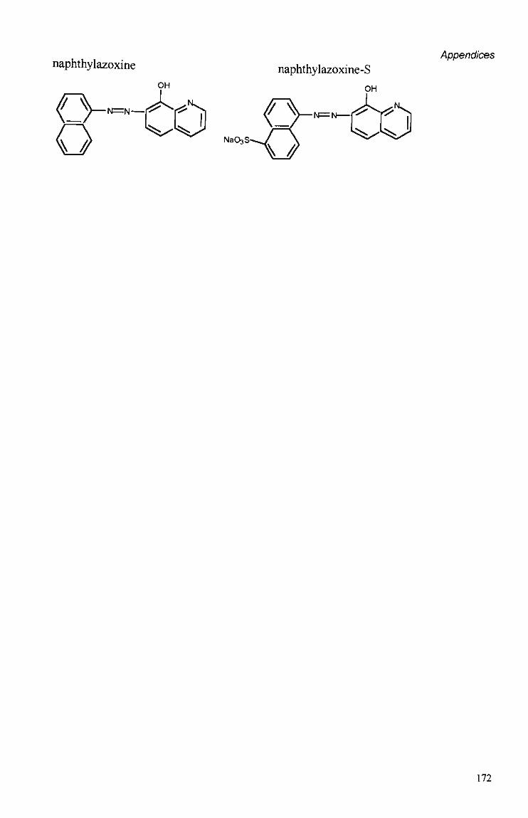
Appendices naphthylazoxine naphthylazoxine-S

172

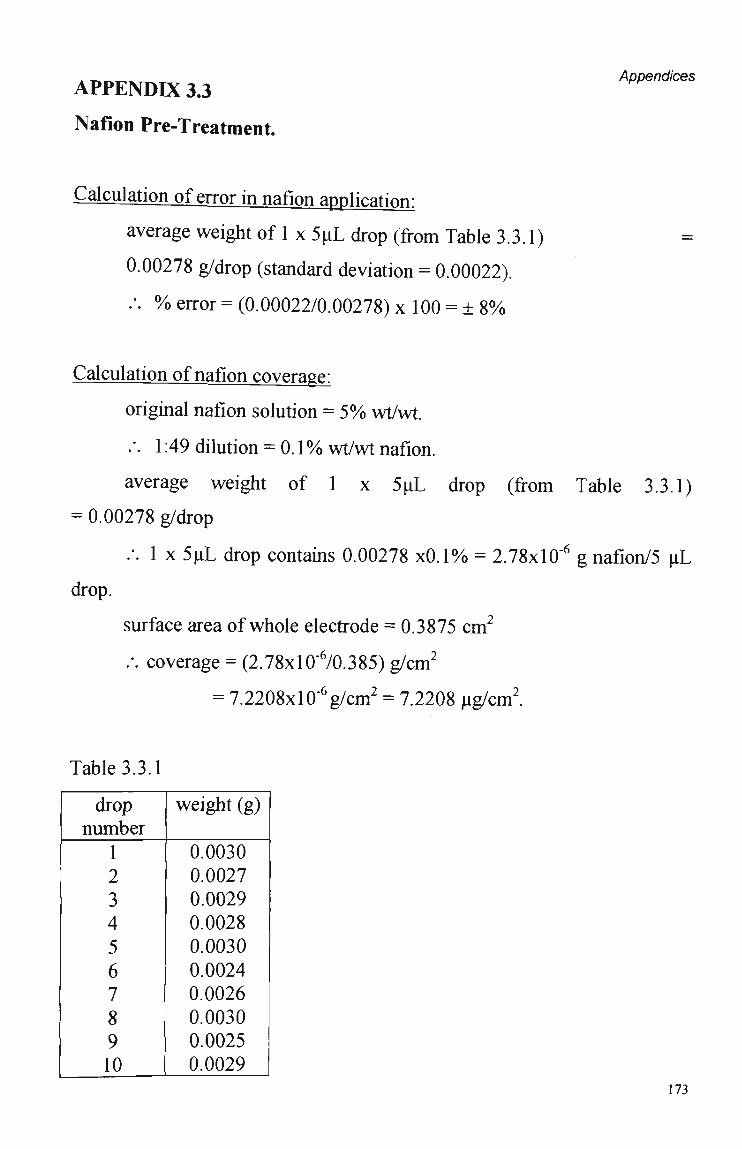
A P P E N D I X 3.3

Nafion Pre-Treatment.

Appendices

Cálculation of error in nafion application-

average weight of 1 x 5 uL drop (from Table 3.3.1)

0.00278 g/drop (standard deviation = 0.00022).

.'. % error = (0.00022/0.00278) x 100 = ± 8 %

Cálculation of nafion coverage:

original nafion solution = 5 % wt/wt.

.*. 1:49 dilution = 0.1% wt/wt nafion.

average weight of 1 x 5uL drop (from Table 3.3.1)

= 0.00278 g/drop

.-. 1 x 5pL drop contains 0.00278 x0.1% = 2.78xl0"6 g nafion/5 uL

drop.

surface área of whole electrode = 0.3875 cm2

.-. coverage = (2.78xl0"6/0.385) g/cm2

= 7.2208x10-6 g/cm2 = 7.2208 ug/cm2.

Table 3.3.1

drop number

1 2 3 4 5 6 7 8 9 10

weight (g)

0.0030 0.0027 0.0029 0.0028 0.0030 0.0024 0.0026 0.0030 0.0025 0.0029

173

APPENDIX 5.1

Peak Ratios

Appendices

The peak ratio is a unit-less number which expresses the relative

selectivities of polymers for various analytes.

Calculating this value has two effects:

(1) removes the units and therefore allows the comparison of polymers

with very different sensitivities.

(2) when plotted allows the simple visual analysis of the effects of

changing detection parameters (eg, Figure 5.4, where it is immediately

obvious that the 0.0 V to -0.8 V potential range gives the greatest relative

selectivity change for the N 0 3 analyte).

174

Appendices

A P P E N D I X 5.2

Data and report for PCA, Figure 5.3

Peak Ratios for Cations/Li over four different potential waveforms, for five different polymers. Current sample time = 100 msec on the upper potential limit. Potential Waveform

-0.4 V to O.OV

-0.4 V to -0.8 V

O.OV to 0.5 V

0.0 V to 0.25 V

Cation/ Li

Na/Li NHVLi K/Li Mg/Li Ca/Li

Na/Li NFL/Li K/Li Mg/Li Ca/Li

Na/Li NH4/LÍ K/Li Mg/Li Ca/Li

Na/Li NH4/LÍ K/Li Mg/Li Ca/Li

PP/Cl

1.60 1.60 1.88 1.58 1.63

1.77 1.67 2.22 1.23 1.36

1.59 1.11 1.75 2.21 2.38

1.81 3.13 2.25 1.19 1.28

PP/SO4

1.39 1.32 1.79 0.86 0.67

1.28 0.78 1.33 0.50 0.50

2.00 1.54 1.86 2.23 2.14

1.44 2.75 1.81 0.13 -0.38

PP/NO3

1.42 1.16 1.55 1.16 1.16

1.52 1.00 1.71 1.12 1.12

1.94 1.00 1.69 2.69 2.44

1.64 1.72 1.96 1.04 1.28

PP/DS

1.64 1.64 1.89 1.58 1.67

1.58 1.47 2.09 1.24 1.56

1.56 1.07 1.75 1.72 2.06

1.93 3.20 2.47 1.40 1.60

PP/MSA

1.82 1.24 2.20 0.49 0.65

1.76 0.42 1.94 0.30 0.57

2.22 3.00 2.83 3.06 3.11

2.31 3.77 3.23 -0.23 -0.38

Analyte concentrations were: 0.5 ppm Fluoride; 0.75 ppm Chloride; 3.75 ppm Sulphate; 2.50 ppm Nitrate, 3.75 ppm, Phosphate, 1 ppm Lithium; 4 ppm Sodium; 10 ppm Ammonium; 10 ppm Potassium; 5 ppm Magnesium; 10 ppm Calcium

Principal Component Analysis PCI PC2 PC3 PC4

Eigenvalue 11.668 6.309 1.694 0.329 Proportion 0.583 0.315 0.085 0.016 Cumulative 0.583 0.899 0.984 1.000

175

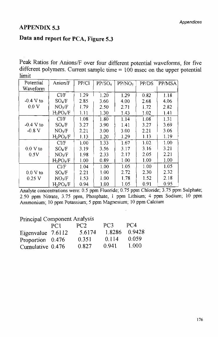
A P P E N D I X 5.3

Data and report for PCA, Figure 5.3

Appendices

Peak Ratios for Anions/F over four different potential waveforms, for five different polymers. Current sample time = 100 msec on the upper potential limit

Potential Waveform

-0.4 V to O.OV

-0.4 V to -0.8 V

0.0 V to 0.5V

0.0 V to 0.25 V

Analvte conce

Anion/F

Cl/F SO4/F NO3/F H2P04/F Cl/F SO4/F NO3/F H2P04/F Cl/F SO4/F NO3/F H2P04/F Cl/F SO4/F NO3/F H2P04/F

intrations w<

PP/Cl

1.29 2.85 1.79 1.11 1.08 3.27 2.21 1.13 1.00 3.19 1.98 1.00 1.04 2.21 1.53 0.94

;re: 0.5 pt

PP/S04

1.20 3.60 2.50 1.30 1.80 3.90 3.00 1.20 1.33 3.56 2.33 0.89 1.00 1.00 1.00 1.00

>m Fluoric

PP/NO3

1.29 4.00 2.71 1.43 1.14 1.41 3.00 1.29 1.67 3.17 2.17 1.00 1.05 2.72 1.78 1.05

e; 0.75 pp

PP/DS

0.82 2.68 1.72 1.02 1.08 3.27 2.21 1.13 1.02 3.16 2.05 1.00 1.00 2.30 1.52 0.91

m Chlorid

PP/MSA

1.18 4.06 2.82 1.41 1.31 3.69 3.06 1.19 1.00 3.21 2.21 1.00 1.05 2.32 2.18 0.95

s; 3.75 ppr 2.50 ppm Nitrate, 3.75 ppm, Phosphate, 1 ppm Lithium; 4 ppm Sodium; 10 ppm Ammonium; 10 ppm Potassium; 5 ppm Magnesium; 10 ppm Calcium

Principal Component Analysis PCI PC2

Eigenvalue 7.6112 5.6174 Proportion 0.476 0.351 Cumulative 0.476 0.827

PC3 PC4 1.8286 0.9428 0.114 0.059 0.941 1.000

176

Appendices

APPENDIX 7.1

Report for PLS, Figure 7.2

Number of Cross-validation Groups: 39 Optimal Number of Components: 18

Goodness-of-Fit and Goodness-of-Prediction

Comp Residuais S 1 2 3 4 5 6 7 8 9 10 11 12 13 14 15 16 17 18

16980 7234 6819 5853 3662 3000 2135 1423 1204 892.8 660.8 557.0 410.5 291.5 237.1 143.4 129.3 110.5

R2 0.6184 0.8374 0.8467 0.8685 0.9177 0.9326 0.9520 0.9680 0.9729 0.9799 0.9851 0.9875 0.9908 0.9934 0.9947 0.9968 0.9971 0.9975

Resid PRESS 21739 10633 10609 10585 8906 8241 6513 6304 5775 5628 5006 4604 4265 4015 3987 3933 3714 3577

R2(cross validated) 0.5115 0.7611 0.7616 0.7621 0.7998 0.8148 0.8536 0.8583 0.8702 0.8735 0.8875 0.8965 0.9042 0.9098 0.9104 0.9116 0.9165 0.9196

177

^ _ References

REFERENCES

1 D. Diamond, Electroanalysis, 5, 1993, 795-802.

2 W.P. Carey, Trends In Analytical Chemistry, 13(5), 1994, 210-Z Io.

3 T. Kunt, L. Ratton, T. McAvoy, T. Fuja, S. Semancik and R. Cavicchi, Computers Chem. Engng, 20, 1996 Suppl. S1437-S1442.

4 N. Ryman-Tubb, Expert Systems, 12(2) 1995, 157-161.

5 J.W. Gardner and P.N. Bartlett, Sensors and Actuators B, 18-19, 1994,211-220.

6 J.W. Gardner and P.N. Bartlett, Sensors and Actuators B -Chemical, 33(1-3), 1996, 60-67.

7 M.P. Byfield, I.P. May, GEC Journal of Research, 13(1), 1996, 17-27.

8 SENSE 1(2), 1996; (a) "Automated Quality Evaluation of Shrimp Using the e-NOSE.", pi; (b) "Quality Control of Cheese Using the e-NOSE 4000.", p5.

9 MA. Craven, J.W. Gardner and P.N. Bartlett, Trends in Analytical Chemistry, 15(9), 1996,486-493.

10 J.B. Tomlinson, I.H.L. Ormrod and F.R. Sharpe, Journal of the American Society ofBrewing Chemists, 53(4), 1995, 167-173.

11 D. Hodgins and D. Simmonds, Journal of Automatic Chemistry, 17(5), 1995, 179-185.

12 F. Winquist, E.G. Hormsten, H. Snudgren and I. Lundstrom, Measurement Science and Technology, 4(12), 1993, 1493-1500.

13 S. Singh, E.L. Hines and J.W. Gardner, Sensors and Actuators B -Chemical, 30(3), 1996, 185-190.

178

References

14 N. Togari, A. Kobayashi and T. Aishima, Food Research International, 28(5), 1995, 495-502.

15 T.C. Pearce, Biosystems, 41(2), 1997, 69-90.

16 T.H. Musselbrook, P.J. Hobbs and K.C. Persaud, Journal of Agricultural Engineering Research, 66(3), 1997, 213-220.

17 S.S. Schifônan, B.G. Kermani and H.T. Nagle, Chemical Senses, 22(2), 1997,119-128.

18 A. Jonsson, F. Winquist, J. Schunurer, H. Sundgren and I. Lundstrom, International Journal of Food Microbiology, 35(2), 1997, 187-193.

19 E.L. Kalman, F. Winquist and I. Lundstrom, Atmospheric Environment, 31(11), 1997, 1715-1719.

20 T. Borjesson, T. Ekiov, A. Jonsson, H. Sundgren and J. Schnurer, Cereal Chemistry, 73(4), 1996, 457-467.

21 P.J. Hobbs, T.H. Misselbrook and B.F. Pain, Journal of Agricultural Engineering Research, 60(2), 1995, 137-144.

22 A. Coghlan, New Scientist, 141(1911), 20, 1994.

23 M. Holmberg, F. Winquist, I. Lundstrom, J.W. Gardner and E.L. Hines, Sensors and Actuators B - Chemical, 27(1-3), 1995, 246-249.

24 M. Josowicz and P. Topart 1992, Sensors and Sensory Systems for an Electronic Nose, 117-129, J.W. Gardner and P.N. Bartlett (Eds), Kluwer Academic Pubüshers, the Netherlands.

25 M.C. Lonergan, E.J. Severin, B.J. Doleman, S.A. Beaber, R.H. Grubbs and N.S. Lewis, Chem Mater. 8, 1996, 2298-2312.

26 G. Taubes, Discover, Sept 1996, 40-50 (article on Grubbs and Lewis's "Electronic Nose").

27 M.S. Freund and N.S. Lewis, Proc. Natl. Acad. Sei USA, 92(7), 1995, 2652-2656.

179

_ References

28 A.Q. Contractor, H Sangodkar, S. Sukeerthi, R.S Srinivasa and R. Lal, Analytical Chemistry, 68(5), 1996, 779-783.

29 A.Q. Contractor, T.N. Sureshkumar, R. Narayanan, S. Sukeerthi. R. Lal and R.S. Srinivasa, Electrochimica Acta, 39, 1994, 1321-1324.

30 K. Suzuki and T. Takada, Sensors and Actuators B, 25, 1995, 773-776.

31 A.C Partridge, P. Harris, and M.K. Andrews, Analyst, 121, 1996, 1349-1353.

32 V.P. Grigorian, Neftyanoe Knozyaistvo, 2, 1997, 6-9.

33 J.M. Slater, J. Paynter and EJ. Watt, Analyst, 118, 1993, 379-384.

34 F. Selampinar, L. Toppare, U. Akbulut, T. Yalcin and S. Suzer, Synthetic Metals, 68. 1995, 109-116.

35 D. Hodgins, Sensors and Actuators B - Chemical, 27(1-3), 1995, 255-258.

36 J.V. Hatfield, P. Neaves, P.J. Hicks, K. Persand and P. Travers, Sensors and Actuators B - Chemical, 18(1-3), 1994, 221-228.

37 J.R. Setter, P.C. Jurs, S.L. Rose, Analytical Chemistry, 58, 1986, 860-866.

38 J. Wang, G.D. Rayson, L. Ziling and W. Hui, Analytical Chemistry, 62, 1990, 1924-1927.

39 X. Wang, S. Yee and P. Carey, Sensors and Actuators B, 13-14, 1993,458-461.

40 J. Wang, Q. Chen, G. Rayson, B. Tian and Y. Lin, Analytical Chemistry, 65, 1993, 251-254.

41 C. Di Natale, FA.M Davide, A. D'Amico, G. Sberveglieri, P. Nelli, G. Faglia and C. Perego, Sensors and Actuators B, 24-25, 1995, 801-804.

180

. References 42 X.D. Wang, W. P. Carey, S.S Yee, Sensors and Actuators B -

Chemical, 28(1), 1995, 63-70. 43 RJ. Forster and D. Diamond, Analytical Chemistry, 64, 1992,

1721-1728.

44 D. Diamond, J.M. Lu, Q. Chen and J. Wang, Analytica Chimica Acta, 281(3), 1993,628-635.

45 S. Iiyama, Y. Miyazaki, K. Hayashi, K. Toko, K. Yamafuji, H. Ikezaki and K. Sato, Sensors and Materials, 4(1), 1992, 21-27.

46 Y. Kikkawa, K. Toko and K. Yamafugi, Sensors and Materials, 5(2) 1993, 83-90.

47 K. Toko, T. Matsuno, K. Yamafuji, K. Hayashi, H. Dcazaki, K. Sato, R. Toukubo and S. Karawarai, Biosensors and Bioelectronics, 9, 1994, 359-364.

48 K. Hayashi, K. Toko, M. Yamanaka, H. Yoshihara, K. Yamafuji, H. Ikazaki, R. Toukubo and K. Sato, Sensors and Actuators B, 23, 1995,55-61.

49 K. Toko, T. Murata, T. Matsuno, Y. Kikkawa and K. Yamafuji, Sens. AndMater., 4, 1992, 145-151.

50 Y. Kanai, M. Shimizu, H. Uchida, N. Nakahara, CG. Zhou, H. Maekawa and T. Katsube, Sensors and Actuators B, 20, 1994, 175-179.

51 S. Iiyama, M. Yahiro and K. Toko, Sensors and Materials, 7(3), 1995, 191-201.

52 Y. Arikawaa, K. Toko, H. Ikezaki, Y. Shinha, T. Ito, I. Oguri and S. Baba, Sensors and Materials, 7(4), 1995, 261-270.

53 S. Iiyama, S. Ezaki, K. Toko, T. Matsuno and K. Yamafuji, Sensors and Actuators B, 24-25, 1995, 75-79.

54 Y. Sasaki, Y. Kanai, H. Uchida and T. Katsube, Sensors and Actuators B, 24-25, 1995, 819-822.

55 K. Toko, T. Matsuno and K. Yamafuji, Japanese Journal of AppliedPhysics, 32, 1993, 5731-5736.

181

References

56 K. Toko, T. Iyoto, Y. Mizota, T. Matsuno, T. Yoshioka, T. Doi, S. Iiyama, T. Kato, K. Yamafuji and R. Watanabe, Jpn. J Appl. Phys., 34, 1995, 6287-6291.

57 S. Iiyama, K. Toko, T. Matsuno and K. Yamafugi, Chemical Senses, 19(1), 1994,87-96.

58 S.L. Rose-Pehrsson, J.W. Grate, D.S. Ballantine and P.C. Jurs, Analytical Chemistry, 60, 1988, 2801-2811.

59 M. Rapp, B. Boss, A. Voight, H Gemmeke and HJ. Ache FreseniusJ. Analytical Chemistry, 352, 1995, 699-704.

60 E.T. Zellers, S.A. Batterman, M. Han and SJ. Patrosh, Analytical Chemistry, 67, 1995, 1092-1106.

61 Z. Deng, D.C. Stone and M. Thompson, Analyst, 121, 1996, 1341-1348.

62 M. Ohnishi, T. Ishibashi, M. Aoki and C. Ishimoto, Japanese Journal of Applied Physics, Part 1 - Regular Papers Short Notes and Review Papers, 33(10), 1994, 5981-5986.

63 J. Auge, P. Hauptmann, J. Hartmann, S. Rosler and R. Lucklum, Sensors and Actuators B, 26-27,1995,181-186.

64 P. Hauptmann, R Lucklum, J. Hartmann, J. Auge and B. Adler, Sensors and Actuators A- Physical, 37, 1993, 309-316.

65 H. Nanato, S. Tsubakino, M. Dceda and F. Endo, Sensors and Actuators B, 24-25, 1995, 794-796.

66 Z. Cao, H.G. Lin, B.F. Wang, D. Xu and R.Q. Yu, Fresenius J Analytical Chemistry, 355, 1996, 194-199

67 H.H. Wang, BiotechAdv., 11, 1993, 701-710.

68 B.W. Saunders, D.V. Theil and A. Mackay-Sim, Analyst, 120, 1995, 1013-1018.

182

PpAsrpnpp c

69 A. Mackay-Sim, T.R. Kennedy, G.R. Bushell and D.V. Thiel, Analyst, 118, 1993, 1393-1398.

K.D. Schierbaum, A. Gerlach, M. Haug and W. Gopel, Sensors and Actuators A, 31, 1992, 130-137.

71 J.M. Slater, EJ. Watt, NJ. Freeman, I.P. May and DJ. Weir Analyst, 117, 1992, 1265-1270.

72 R Zhou, U Weimar, K.D. Schierbaum, K.E. Geckeler and W. Gopel, Sensors and Actuators B-Chemical, 26, 1995, 121-125

73 K.D. Schierbaum and W. Gopel, Synthetic Metals, 61, 1993, 37-45.

74 C. Dinatale, JAJ. Brunink, F. Bungaro, F. Davide, A. Damico, R. Paolesse, T. Boshi, M. Faccio and G. Ferri, Measurement Science and Technology, 7(8), 1996, 1103-1114.

75 J. White, J.S. Kauer, TA Dickinson and D.R. Walt, Analytical Chemistry, 68, 1996, 2191-2202.

76 P. Pântano and D.R. Walt, Analytical Chemistry, 67, 1995, 481-487A.

7 B.G. Healey and D.R. Walt, Analytical Chemistry, 67, 1995, 4471-4476.

78 K.S. Bronk and D.R. Walt, Analytical Chemistry, 66, 1994, 3519-3520.

79 TA. Dickinson, J. White. J.S. Kauer and D.R. Walt, Nature, 382, 1996, 697-700.

80 D.R. Walt, V. Agayn, K. Bronk and S. Barnard, Applied Biochemistry and Biotechnology, 41, 1993, 129-138.

81 C.K. Chiang, CR. Fincher, Y.W. Park, AJ. Heeger, H. Shirakawa, EJ. Louis, S.C Gau and A.G. Macdiarmid, Phys. Rev. Lett. 39, 1977, 1098.

82 D. J. Walton, Materials and Design, 11(3), 1990, 142-152.

183

References

83 G.G. Wallace, Materials Fórum 16, 1992, 111-115.

84 P.R. Teasdale and G.G. Wallace, Chimica Oggi, October 1994, 19-24.

85 R. Noufi, AJ. Frank and AJ. Nozik, J Am. Chem. Soe, 103, 1981, 1849-1850.

86 F.F. Fan, B.L. Wheeler, AJ Bard and R.N. Noufi, J Electrochem. Soe, 128(9), 1981, 2042-2045.

87 AJ. Frank and K. Honda, J Phys. Chem., 86, 1982, 1933-1935.

88 T. Skotheim, I. Lundstrom and J. Prejza. J. Electrochem. Soe, Julyl981, 1625-1626.

89 J.W. Gardner and P.N. Bartlett, Nanotechnology, 2, 1991, 19-32.

90 S. Roth, W. Graupner and P. McNeillis, Acta Physica Polonica A, 87(4-5), 1995,699-711.

91 B. Zinger and L.L. Miller, J Am. Chem. Soe, 106, 1984, 6861-6863.

92 L.L. Miller, B. Zinger and Q. Zhou, J. Am. Chem. Soe, 109, 1987, 2267-2272.

93 R.L. Blankespoor and L.L. Miller, J. Chem. Soe, Chem Commun., 1985, 90-92

94 M. Pyo, G. Maeder, R.T. Kennedy and J.R. Reynolds, J. Electroanal. Chem., 368, 1994, 329-332.

95 L.H.M. Krings, E.E. Havinga, J.J.T.M. Donkers and F.T.A. Vork, Synthetic Metals, 54, 1993, 453-459.

96 N. Mermilloid, J. Tanguy and F. Petiot, J. Electrochem. Soe, 133(6), 1986, 1073-1079.

97 A. Mohammadi, O. Inganas and I. Lundstrom, J. Electrochem. Soc.,133(5), 1986, 947-949.

184

References

98 PJ. Riley and G.G. Wallace, MaterialsAustralasia, 1991, 12-13.

99 R.C.D. Peres, V.F. Juliano, M. De Paoli, S. Panero and B. Scrosati, Electrochimica Acta, 38(7), 1993, 869-876.

100 C. Kranz, M. Lugwig, H.E. Gaub and W. Schuhmann, Adv. Mater., 7(6)1995, 568-571.

101 P. Pântano and W.G. Kuhr, Electroanalysis, 7(5), 1995, 405-415.

102 H. Sangodkar, S. Sukeerthi, R.S. Srinivasa, R. Lal and A.Q. Contractor, Analytical Chemistry, 68, 1996, 7779-783,

103 H. Sangodkar, S. Sukeerthi, R.S. Srinivasa, R. Lal and A.Q. Contractor, Anal. Chem, 68(5), 1996, 779-783.

104 S. Sukeerthi and A.Q. Contractor, Indian J. of Chemistry, 33(6), 1994,565-571.

105 P. Burgmayer and R.W. Murray, J Am. Chem. Soe 104, 1982, 6139-6140.

106 I. Loh, R.A. Moody and J.C. Huang, Journal of Membrane Science, 50, 1990,31-49.

107 P. Burgmayer and R.W. Murray, J Phys. Chem. 88, 1984, 2515-1521.

108 W.E. Price et ai. 1994, Frontiers of Polymers and Advanced Materials, Plenum Press, New York, 599-605.

109 H. Zhao, 1993, PhD Thesis, Wollongong University.

110 P.M. Beadle, L. Rowan, J. Mykytiuk, N.C. Billingham and S.P. Armes, Polymer, 34(7), 1993, 1561-1563.

111 T.F. Otero, E. Angulo, J. Rodriguez and C Santamaria, J. Electroanal Chem. 341, 1992, 369-375.

112 A.F. Diaz and J.C. Lacroix, J Chem., 12(4) 1988, 171-180.

185

113 R. John, 1992, PhD Thesis, University of Wollongong.

114 R.C.D. Peres, MA. DePaoli and R.M. Torresi, Synthetic Metals, 48, 1992,259-270.

115 C. Barbero, M.C Miras, R. Kotz and O. Haas, Solid State Ionics, 60, 1993, 167-172.

116 J. Lippe and R. Holze, Molecular Crystals and Liquid Crystals, 208, 1991, 99-109.

117 H. Kaufinan, K. K. Kanazawa and G. B. Street; Phys. Rev. Lett., 53,1984,2461.

118 Q. X. Zhou, C J. Kolaskie and L. L. Miller; J Electroanal. Chem., 223,1987, 283.

119 P. Marque, J. Roncali and F. Garnier; J. Electroanal. Chem., 218, 1987, 107.

120 K. Naoi, M. Lien and W.H. Smyrl, J Electrochem. Soe, 138(2) 1991, 440-445.

121 I.C Lee, J Electroanal. Chem., 340, 1992, 333-339.

122 B. Yan, J. Yang, Y. Li and R. Qian, Synthetic Metals, 58, 1993, 17-27.

123 X. Chen, J. Devaux, J.P. Issi and O. Billand, Polymer Engineering and Science, 35(8), 1995, 642-647.

124 N. M. Ratcliffe, Synthetic Metals, 38, 1990, 87-92.

125 A.F. Diaz and JA. Logan, J. Electroanal. Chem., 111, 1980, 111.

126 L. Groenendaal, H.W.I. Peerlings, J.L.J. van Dongon, E.E. Havings, J.A.J.M. Vekemans and E.W. Meijer, Macromolecules, 28,1995,116.

127 WA. Wampler, K. Rajeshwar, R.G. Pethe, R.C Hyer and S.C Sharma. Jof Materials Research, 10(7), 1995,1811-1822..

186

References

128 G. Zebi, M. Veronelli, S. Martina, A.D. Schluter and G. Wegner, Adv. Mater. 6, 1994, 385.

129 S.N. Tan and H. Ge, Polymer, 37(6), 1996, 965-968.

130 J.C. Thieblemont, J.L. Gabelle and M.F. Planche, Synthetic Metals, 66(3), 1994, 243-247.

131 M.M. Ayad, J. of Applied Polymer Science, 53(10), 1994, 1331-1337.

132 M.F Planche, J.C. Thieblemont, N. Mazars and G. Bidan, J. of Applied Polymer Science, 52(13), 1994,1867-1877.

133 S. Maiti, Indian J Chem., 33A, 1994, 524-539.

134 T.F. Otero and E. de Larreta-Azelain, Synthetic Metals, 26,1988, 79

135 T.F. Otero and C Santamaria, Synthetic Metals, 51, 1992, 313-319.

136 G.R. Mitchell and A. Geri, JPhys. D. Appl. Phys., 20, 1987, 1346.

137 R. Qian and J. Qiu, Polymer Journal, 19(1), 1987, 57-172.

138 A Talaie and G.G. Wallace, Synthetic Metals, 63, 1994, 83-88.

139 H. An, Y. Haga, T. Yuguchi and R. Yosomiya, Die Angewadte Makromolekulare Chemie., 218,1994,137-151.

140 A. F. Diaz and B. Hall, IBMJ Res. Develop., 27(4),1983 .

141 M.D. Imisides, R. John. P. Riley and G.G. Wallace, Electroanal. 3, 1991,879.

142 C.K. Baker and J.R. Reynolds, J Electroanal. Chem., 251, 1988, 307-322.

143 Y. Lin and G.G. Wallace, Electrochimica Acta, 10, 1994, 1409-

1413.

187

References

144 J. Lukkari, Materials Science Fórum, 191, 1995, 219-224.

145 F. Beck, Electrochimica Acta, 33(7), 1988, 839-850.

146 CP. Andrieux, P. Audebert, P. Hapiot and J.M. Saveant, J Phys. Chem., 95, 1991, 10158-10164.

147 A. Diaz and J. Bargon 1986 Handbook of Conducting Polymers Volume 1, T.A. Skotheim, Ed., 1986, p82.

148 R. John and G.G. Wallace, Polymer International, 27, 1992, 255-260.

149 R. John and G.G Wallace, J. Electroanal. Chem., 306, 1991, 157-167

150 E.M. Genies, G. Bidan and A.F. Diaz, J Electroanal. Chem., 149, 1983,101-113.

151 D.F. Diaz, J. Crowley, J. Bargon, G.P. Gardini and J.B. Torrance, J. Electroanal. Chem., 121,1981, 355-361.

152 M.S. Kiani and G.R. Mitchell, Synthetic Metals, 48, 1992, 203-218.

153 J. Ruhe, T. A. Ezquerre, G. Wegner, Synthetic Metals, 28, 1989, 177.

154 J. C Scott, J.L Bredas, K. Yakaushi, P. Pfluger and G.B. Street, Synthetic Metals, 9, 1984, 165-172.

155 J.C. Scott, P. Pfluger, M.T. Krounbi and G.B. Street, Physical Review B,2H, 1983,2140.

156 G.G. Wallace, Chemistry In Britain, November 1993, 967-970.

157 P.R. Teasdale and G.G. Wallace, Analyst, 118, 1993, 329-334.

158 W. Lu and G.G. Wallace, Electroanalysis, 9(4), 1997, 1-7.

159 O. Sadik and G.G. Wallace, Anal Chim. Acta., 279,1993, 209.

188

References

160 P.N. Bartlett and R.G. Whittaker, J Electranal. Chem., 224, 1987, 27.

161 P.N. Bartlett, P. Tebbutt and R.G. Whittaker, Prog. React. Kinet., 16,1991,55.

162 S. Adelojou, S. Shaw and G.G. Wallace, Electroanalysis, 6, 1994, 865-870.

163 D. Barnett, D.G. Laing, S. Skopec, O. Sadik and G.G. Wallace, Analytical Letters, 27(13), 1994, 2417-2429.

164 P.N. Bartlett and J.M. Cooper, J Electroanal. Chem.,.362, 1993, 1.

165 CR. Martin, Science, 266, 1994, 1961.

166 J.N. Barisci, C Conn and G.G. Wallace, Trends in Polymer Science, 4(9), 1996, 307-311.

167 G. Erdogdu and A.E. Karagozler, Talanta, 44(11), 1997, 2011-2018.

168 Y. Ikariyama and W.R. Heineman, Analytical Chemistry, 58, 1986, 1803-1806.

169 O. Sadik and G.G. Wallace, Electroanalysis, 5, 1993, 555.

170 J. Yen and R. Baldwin, Analytical Chemistry, 58, 1988, 1982.

171 R.C Martinez, F.B. Dominguez, F.M. Gonzalez, J.H. Medez and R.C. Orellana, Anal. Chim. Acta., 279, 1993, 299-307.

172 I. Lahdesmalci, A. Lewenstam and A. Ivaska, Talanta, 43, 1996, 125-134.

173 Y. Lin and G.G. Wallace, Anal Chim. Acta., 263,1992, 71-75.

174 O. Sadik and G.G. Wallace, Electroanalysis, 6, 1994, 860-864.

175 JJ. Miasik, A. Hooper and B.C. Tofield, J. Chem. Soe Faraday Trans. 7,82,1986,1117-1126.

189

References

176 Y. Lin and G. G. Wallace, Analytical Letters., 22, 1989, 669.

177 Y. Lin and G.G. Wallace, JElectroanal. Chem., 247, 1988, 145.

178 M.E.G. Lyons, W. Breen and J.F. Cassidy, J Chem. Soe Faraday Trans., 87, 1991, 115.

179 M.E.G. Lyons, CH. Lyons, D.E. McCormack, TJ. McCabe, W. Breen and J.F. Cassidy, Anal. Proe, 28, 1991, 104.

180 M.E.G. Lyons, P.N. Bartlett, CH. Lyons, W Breen and J.F. Cassidy, J. Electroanal. Chem., 304, 1991, 1-6.

181 H.L. Ge, O.L. Ho and X.H. Yang, Environmental Monitoring and Assessment, 44, 1997, 361-367.

182 N.M. Ratcliffe, Anal Chim. Acta., 239, 1990, 257-262.

183 J.M. Charlesworth, AC. Partridge and N. Garrard, J. Phys. Chem., 97, 1993, 5418-5423.

184 T. Hanawa and H. Yoneyama, Buli. Chem. Soe Japan, 62, 1989, 1710.

185 Y. Kunugi, K. Nigorikawa, Y. Harima and K. Yamashita, J. Chem. Soe, Chem. Commun., 1994, 873-874.

186 S. Dong, Z. Sun and Z. Lu, Analyst, 113, 1988, 1525-1528.

187 RA. Saracens, J.C. Pack and A.G. Ewing, J. Electroanal. Chem., 197, 1986,265-278.

188 R. Hintsche, C Kruse, A. Uhlig, M. Paeschke, T. Lisec, U. Schnakenberg and B. Wagner, Sensors and Actuators B, 26-27, 1995, 471-473.

189 Q. Wu, K. Lee, C. Liu, Sensors and Actuators B, 13-14, 1993, 1-6.

190 L.E. Fosdick, J.L. Anderson, TA. Baginski and R.C Jaeger, Analytical Chemistry, 58,1986, 2750-2756.

190

References

191 E. Hofer, G. Urban, M.S. Spach, I. Schafferhofer, G. Mohr and D. Platzer, American Physiological Society, 1994, H2136-H2144.

192 E. Dempsey, D. Diamond, M.R. Smyth, G. Urban, G. Jobst, I. Moser, E.MJ Verpoorte, A. Manz, H.M. Widmer, K. Rabenstein and R. Freaney, Anal. Chim Acta, 346(3), 1997, 341-349.

193 A.M. Bond, M. Fleischmann and J. Robinson, J. Electroanal. Chem, 172, 1984, 11-25.

194 S. Pons and M. Fleischmann, Analytical Chemistry, 59(24), 1987, 1391A-1399A. and references contained therein.

195 R.M. Wightman, Science, April 1988, 415-420.

196 R.M. Wightman, Analytical Chemistry, 53, 1981, 1125A.

197 J.C. Myland and K.B. Oldham, J Electroanal. Chem., 347, 1993, 49-91.

198 A.M. Bond, K.B. Oldham and CG. Zoski, J. Electroanal. Chem., 245, 1988, 71-104.

199 A.M. Bond, M. Fleischman and J. Robinson, J. Electroanal Criem., 168,1984,299-312.

200 J.O. Howell and M.K. Wightman, Analytical Chemistry., 56, 1984,524-529.

201 S. Bruckenstein, Analytical Chemistry, 59, 1987, 2098-2101.

202 K.B. Oldham, J. Electroanal Chem., 337, 1992, 91-126.

203 W.L. Caudill, J.O. Howell and R.M. Wightman, Analytical Chemistry, 54, 1982, 2532-2535.

204 R. John and G.G. Wallace, J Electroanal. Chem., 283, 1990, 87-98.

205 K.M. Cheung, D. Bloor and G.C Stevens, Polymer, 29, 1988, 1709-1717.

191

References

206 B. Yan, J. Yang, Y. Li and R. Qian, Synthetic Metals, 58, 1993, 17-27.

207 T. Fang, M. McGrath, D. Diamond and M.R. Smyth, Analytica Chimica Acta, 305, 1995, 347-358.

208 J.C. Hoogvliet, J.M. Reijn and W.P. Van Bennekom, Analytical Chemistry, 63, 1991,2418.

209 T. Matsue, A. Aoki, E. Ando and I. Uchida, Analytical Chemistry, 62, 1990, 407-409.

210 MJ. Mcgrath, E.L Iwuoha, D. Diamond and M.R. Smyth, Biosensors andBioelectronics, 10, 1995, 937-943.

211 T. Fang, M. Mcgrath, D. Diamond and M.R. Smyth, Anal. Chim Acta, 305, 1995,347-358.

212 MJ. Mcgrath, T. Fang, D. Diamond and M.R. Smyth, Analytical Letters, 28(4), 1995, 685-696.

213 W.P. Carey, K.R. Beebe and B.R. Kowalski, Analytical Chemistry, 58, 1996, 149-153.

214 B.R. Kowalski and C.F. Bender, J Am. Chem. Soe, 94(16), 1972, 5632-5639.

215 D.L. Massart and A. Thielemans, Chimia, 39(7/8), 1995, 236-242.

216 S.N. Deming and S.L. Morgan 1993, Data Handling in Science and Technology - Volume 11: Experimental Design: A Chemometric Approach, 2nd Edition, Elsevier Science Pubüshers, the Netherlands.

217 D.L Massart B.G.M. Vandeginste, S.N. Deming, Y. Michotte and L. Kaufman, 1989, Data Handling in Science and Technology -Volume 2: Chemometrics: A Textbook, Elsevier Science Pubüshers, the Netherlands.

192

References

218 M A . Sharaf, D.L. Illman and B.R. Kowalski 1986, Chemical Analysis - Volume 82: Chemometrics, John Wiley and Sons Inc., Toronto.

219 M. Meloun, J. Militky and M. Forina 1994, Chemometrics for Analytical Chemistry - Volume 2: PC-Aided Regression and Related Methods, Elüs Horwood - Prentis Hall PTR, Sydney.

220 M. Mellinger, Chemometrics and Intelligent Laboratory Systems, 2, 1987, 29-36.

221 S.D. Brown and R.S. Bear, Criticai Reviews in Analytical Chemistry, 24(2), 1993, 99-131.

222 S.D. Brown, R.S. Bear and T.B. Blank, Analytical Chemistry, 64, 1992, 22R-49R.

223 S.D. Brown, T.B. Blank, S.T. Sum and L.G. Weyer, Analytical Chemistry, 66, 1994, 315R-359R.

224 S.D Brown, S.T. Sum. F. Despagna and B.K. Lavine, Analytical Chemistry, 68, 1996, 21R-61R.

225 S. Wold, K. Esbensen and P. Geladi, Chemometrics and Intelligent Laboratory Systems, 2, 1987, 37-52.

226 P. Geladi and B.R. Kowalski, Anal. Chim. Acta, 185, 1986, 1-17.

227 SCAN Software for Chemometric Analysis Reference Manual (Release 1 for Windows) February 1995 by Minitab In8c. (ISBN 0-925636-25-8)

228 R. John, D.M. Ongarato and G.G. Wallace, Electroanalysis, 3(7), 1996, 623-629.

230 Ionpac CS 12 Analytical Column Instruction and Troubleshooting Guide, Dionex Corporation Document 1992, no. 034785.

231 Ionpac AS11 Analytical Column Instruction and Troubleshooting Guide, Dionex Corporation Document 1992, no. 034785.

193

References

232 S.D. Brown, J of Chemometrics, 8(1), 1994, 95-96.

233 F.R. Fan and AJ. Bard, J. Electrochem. Soe, 133, 1986, 301.

234 R.M. Penner and CR. Martin, J. Electrochem. Soe, 132 1985 514.

235 R.M. Penner and CR. Martin, J Electrochem. Soe, 133,1986 310.

236 H. Chriswanto, H.L. Ge and G.G. Wallace, Chromatographia, 37, 1993,423-428.

237 J.R. Reynolds, M. Pyo and Y.Z. Qiu, Synthetic Metals, 55, 1993, 1388-1395.

238 T.W. Lewis, G.G. Wallace, C.Y. Kim and D.Y. Kim, Synthetic Metals, 84, 1997, 403-404.

239 QJ. Xie, S. Kawabata and H. Yoneyama, JElectroanal. Chem. 420, 1997,219-225.

240 H. Yamato, M. Ohwa and W. Wernet, J. Electroanal. Chem., 397, 1995, 163-170.

241 A. Michalaska, K. Maksymiuk and A. Hulanicki, J. Electroanal. Chem., 392, 1995, 63-68.

242 F. Beck and U. Barsch, Synthetic Metals, 55, 1993, 1299-1304.

243 Dionex Advanced Computer Interface Module Installation and

Operation, Dionex Corporation 1992, Document no. 034039.

244 Installation Instruction and Troubleshooting Guide for the Anion

Micromembrane Suppressor-II, Dionex Corporation 1992,

Document no. 034449

194

References

245 Installation Instruction and Troubleshooting Guide for ththe Cation

Micromembrane Suppressor-II, Dionex Corporation 1992,

Document no. 034450.

246 P.C. Innis, 1996, PhD Thesis, University of Technology, Sydney.

195