K£F5"01'3199'5"ftTIt

A LABORATORY STUDY OF SEDIMENTDISTRIBUTION AT CHANNEL BIFURCATION

'.' ."

ATAULHANNAN

/1/111111!f~~~!""UiIIII- ; .I.

DEPARTMENT OF WATER RESOURCES ENGINEERINGBANGLADESH UNIVERSITY OF ENGINEERING & TECHNOLOGY,

DHAKA

NOVEMBER 1995

A LABORATORY STUDY OF SEDIMENTDISTRIBUTION AT CHANNEL BIFURCATION

ATAUL HANNAN

IN PARTIAL FULFILLMENT OF THE REQUIREMENTSFOR

DEGREE OF MASTER OF SCIENCE IN ENGINEERING(WATER RESOURCES)

DEPARTMENT OF WATER RESOURCES ENGINEERINGBANGLADESH UNIVERSITY OF ENGINEERING & TECHNOLOGY,

DHAKA

NOVEMBER 1995

This is to certify that the thesis on A LABORATORY STUDY OF SEDIMENT

DISTRIBUTION AT CHANNEL BIFURCATION has been done by me. Neither of

this thesis nor the part thereof has been submitted elsewhere for the award of any

degree or diploma.

•

ATAUL HANNANCountersigned by the Candidate

CERTIFICATE

t .

•

\(k,-Dr. M. R. KABIRCountersigned by the Supervisor

Prof. M. Monowar Hossain

Mr. A. K. M. Shamsul Hoque

=e~~.Dr. M. A. Matin

Dr. M. R. Kabir

Prof. Ainun Nishat

NOVEMBER 1995

ATAUL HANNAN

We hereby recommend that the thesis presented by

BANGLADESH UNIVERSITY OF ENGINEERING AND TECHNOLOGYDEPARTMENT OF WATER RESOURCES ENGINEERING

Member(Head of the Department )

Member(External)

Member

Member

Chairman of the Committee( Supervisor)

entitled " A LABORATORY STUDY OF SEDIMENT DISTRIBUTIONAT CHANNEL BIFURCATION" be accepted as fulfilling this part ofthe the requirements for the degree of Master of Science in Engineering(WATER RESOURCES).

ABSTRACT

Morphological behavior of bifurcatibns and confluences which are typical features ofrivers and

estuaries are still not properly understood phenomena. Recently a few researchers have done

some work on bifurcation with the help of I-D model which are not developed particularly for

this purpose. In these l-D models the bifurcation phenomena has been represented by'the help

of nodal point relations. The distribution of sediment at bifurcation is a three dimensional

phenomena. It is very difficult to '~et a clear idea of three dimensional problem with the helpf 1 D d I S I . . h' .,.. d . bo - mo e s. 0, to get some mSlg t mto lliC pnenomcn& an process, la oratory

experiment was initiated at the laboratory of Department of Water Resources Engineering,

BUET. As the bifurcation phenomena is a very complicated one, assumptions were made to

make the problem as simple as possible.

After constructing the experimental set-up all the facilities were tested whether they were

working according to simplification. All instruments were calibrated and the model produced

results as .expected. After being satisfied that the experimental set-up was functioning properly,

main experiments were carried out.

Experiments were carried out with two noses representing two different bifurcation conditions.

The first nose gave results which fits well with the theory S2 = k(tJ2J "']. The only differencesS3 q3

was that with the increase of discharges the value of m (nose geometry) did not remain

constant rather it increased. In case of the second nose the value of m increased with discharge

but at a lower rate. Here the calculated normal depths were far a way from the actual normal

depths of the two downstream branches. This is because the shape of the nose created an

additional influence in the model. So, the results of the two noses can not be compared since

the conditions are not the same. But it can be interred trom the resuits that no gen~ral relation

in the case of sediment distribution over the two downstream branches can be expected since it

depends not only on the geometry of the nose but also on the condition of the downstream

branches as compared to nose configuration. Further studies will help in better under standing

the problem since this may be the beginning of such kind of study.

I

'AdKNOWLEDGMENT

The author acknowledges his sincere gratitude and thanks to Dr. M. R. Kabir, Assistant Professor,

Department of Water Resources Engineering, BUET who introduced the author to the interesting

field of sediment' Tr,ansport Technology. The author is really grateful to his s!lpervisor for his

constant encouragement and wise guidance throughout the experimental investigation and during .

the preparation of this thesis.

The author's sincere thanks are also to the numbers of the examination committee, Dr. Ainun

Nishat, I'rofessor of the Water Resources Engineering Department, Dr. M. M. Hossain,'

Professor and Head of the Water Resources Engineering Department, Dr. ,M. A. Matin,

Associate 'Professor of the Water resources Engineering Department, BUET, Dhaka and Mr. A.

K: M. Shamsul Hoque, Chief Engineer, Planning BWDB, Dhaka for their special interest,

valuable suggestions and help on many occasions.

The author also wishes to thank Prof. M de Vries, Dr. Wang, Mr. van Mierlo, P. den Dekker and

lM vanVoorthuizen. Without their help the model would never have been built. The

experiments were carried out together with two M.Sc students of TU Delft R. Roosjen and C.

Zwanenburg. The author wishes to give special thanks to them for their good co-o~eration.

Also thanks to Mr. van der Wal, who spent some his of spare time in helping to start up the

model, and time to time practical advice given by him was very useful.

The author 'also wishes to thank Md. Salim Kaiser, Assistant Foreman Instructor of

Machines~op, BUET for his help'in constructing allthe steel structures in the model. Thanks are

'also due to Mr. Nazimuddin and Mr. Mostofa. for their kind and constant assistance in

performing the laboratory fests.

ATAUL HANNAN

ii

TAJLE OF CONTENTSi

Abstract

Acknowledgment

Table of Contents

Listof Tables

List of Figures

List of Main Symbols

CHAPTER-l INTRODUCTION

1.1 SCOPE OF THE STUDY"

1,2 OBJECTIVES OF'THE RESEARCH

CHAPTER-2 REVIEW OF LITERATlJ1lli

2, I PREVIOUS RESEARCHES

2,1.1 SOME REMARKS

2,2 INCIPIENT MOTION OF SEDIMENT PARTICLES

2.2, I SHIELDS DIAGRAM

2,3 SEDIMENT MOVEMENT IN RIVERS

CHAPTER-3 THEORETICAL CONSIDERATION

3.1 GENERAL CONSIDERATIONS

3,2 THEORETICAL ANALYSIS

, 3.2,1 SINGULAR POINTS,

3,2,2 THE STABILITY OF THE SINGULAR POINTS

CHAPTER-4 EXPERIMENTAL SET-UP

4, I EXPERIMENTAL SET-UP

4,1.1 THE TEMPORARY PART

iii

I

ii

iii

vii

vii '

x

I

2

3

7

7

8

9

II

12

14

15

18

18

"

4,1.1.1 INFLOW ZONE

4.1.1.2 THE CHARACTERISTICS OF THE MAIN BRANCH

4.1.1.3 THE CHARACTERISTICS OF BRANCH 2 AND 3

4.1.1.4 CONFIGURATION OF THE BIFURCATION

,4.1.1.5 SANDTRAPS

4.1.1.6 OUTFLOW SECTION,

4.1.2 THE PERMANENT PA~TI

4.1.2.1 DOWNSTREAM RESERVOIR

4.1.2.2 PUMP

4.1.2.3 PIPE LINEi

4.1.2.4 UPSTREAM RESERVOIR,,i '

4.1.2.5 THE REGULJ).TING AND MEASURING SYSTEM

4.1.2.5.1 THt TAIL GATES

4.1.2.5.2 THE STILLING BASIN AND TRANSITION FLUMES

4.1.2.5.3 THE GUIDING VANES AND TUBES

4.1.2.5.4 THE ApPROACH CHANNEL AND THE REHBOCK

WEIRS

4.1.2.5.5 THE STILLING BASINS CONNECTED WITH

REHBOCK' WEIRS

4.2 THE WATER CIRCUIT

4.3 SEDIMENT CIRCUIT,

4.4 SAND FEEDER

4.5 SEDIMENTS

,4.6 THE MEASURING TECHNIQUES

4.6.1 DISCHARGE MEASUREMENTS

4.6.2 SEDIMENT TRANSPORT MEASUREMENTS

4.6.3 WATER LEVEL MEASUREMENTS

4.6.4 BED LEVEL MEASUREMENTS

4.7 TEST RUNS .

iv

19

19

2020202223

23

23

.23

24

25,

25

2626

26

27

27

28

2828292930

31

32

33

CHAPTER-5 EXPERIMEN~AL PROCEDURE

5.1 BEFORE STARTING THE MODEL FOR EXPERIMENT THE FOLLOWING THINGS

59

6061

- 64

4747

4748

4950

51

52

53

53

54

55

5656

58

WERE DONE 34

5.2 DURING THE EXPERIMENT THE FOLLOWING THINGS WERE DONE 36

5.3 PROBLEMS FACED DURING MODEL CONSTRUCTION, OBSERVATION AND DATA

COLLECTION 42

CHAPTER-7 CONCLUSION AND RECOMMENDATION

v

7.1- CONCLUSION

7.2 RECOMMENDATION FOR FURTHER STUDY

REFERENCES

TABLES

. CHAPtER-6 DATA ANALYSIS, RESULTS AND DISCUSSION

, .

.;l:c FIGURES 71

PLATES 151

APPENDIX-A DETAIL OF THE REHBOCK WEIRS A-I

APPENDIX-B ACCURACY OF THE REHBOCK WEIRS B-1

?,. APPENDIX-C CALIBRATION CHART OF THE BUCKETS C-l

APPENDIX-D PROGRAM TO CALCULATE THE NORMAL DEPTHS 0-1

vi

LIST OF TABLES

TABLE 2.1: ' HYDRAULIC AND SEDIMENT PARAMETERS OF THE NILE RIVER AT

BENI - MAZZAR 64TABLE 6.1 :' RESULTS OF THE FIRST ,NOSE (30 Lis) 65TABLE 6.2: RESULTS OF THE FIRST NOSE (40 Lis) . 66TABLE 6.3: RESULTS OF THE FIRST NOSE (20 Lis) 61TABLE 6.4: . RESULTS OF THE SECOND NOSE (30 Lis) 68'TABLE 6.5: RESULTS OF THE SECOND .NOSE (40 Lis) 69 .. . ,TABLE 6.6': RESULTS OF THE SECOND NOSE (20 Lis) 70

LIST OF FIGURES

FIGURE 1.1 THE CONFLUENCE Al-m BIFURCATION OF RIVER SYSTEM 71

FIGURE 2.1 MODE~ OF THE BENI-LAZZAR REACH OF THE NILE RIVER 724 !

FIGURE 2.2 ALIGNMENT OF THE THREE DREDGED CHANNELS 73

FIGURE 2.3 SCHEMATIZED MAIN AND SECONDARY CHANNELS SYSTEM 14

FIGURE 2.4 SHIELDS DIAGRAM FOR INCIPIENT MOTION .74

FIGURE 3.1 PHASE DIAGRAM IS CASE OF m«5i3) 15

FIGURE 3.2 PHASE DIAGRAM IS CASE OF m >(5/3) 75

FIGURE 4.1, GENERAL LAYOUT OF THE SET-UP 76

vii

-", viii

FIGURE 4.19B CALIBRATION CURVE FOR SAND FEEDER NO.2 91

FIGURE 4.20 THE GRAIN SIZE DISTRIBUTION OF WASHED AND'UNWASHED SAND 92

FIGURE 4.21 DETAIL OF THE STILLING BASINS 93

FIGURE 4.22 DETAIL OF THE SPECIAL PIN 93

r FIGURE 4.23 DETAIL OF THE BED LEVEL MEASUREMENT POINTS 94

FIGURE 4.24 RESULTS OF THE TEST RUNS 95

FIGURE 5.1 LAYOUT OF THE 'PIPE LINE '(FIRST) 96

FIGURE 6.1-6:41 BED LEVEL EVOLUTION 97-137

fFIGURE 6:42-6:47 VARIATIONOF DISCHARGE WITH RUN TIME 138-144

J

FIGURE 6:48-6.53 RELATION BETWEEN SEDIMENT TRANSPORT RATIO AND DISCHARGE

RATIO.

ix

145-150

LIST OF MAIN SYMBOLS

x

.'

xi

CHAPTER-l

INTRODUCTION

Bifurcations and Confluences are typical features of rivers and estuaries. In most cases,

confluences occur in the upstream and bifurcations occur in the downstream of a river in the

delta area, although it is not applicable in all rivers. Braided rivers, in particular, are

.characterized by a repetition of confluence. and bifurcations. In cha.tlllel networks in,

estUaries, confluences turn into a bifurcation at the turn of the tide. Fig. 1.1 shows the

definition sketch of bifurcation and confluence of river.

At a confluence one may know the discharge and the sedim~nt transport in each of the

upstream channels. The discharge and sediment transport in the downstream channel is

simply the sum of those in the upstream channels. At a bifurcation, however, it has to be' ,

determined how the discharge and sediment are distributed over the downstream channel.

The distribution of ,the discharge can easily be determined by the geometry and the,hydraulic resistance of the idownstream channels. Now the problem is to determine the

distributiOll of sediment ov~r the branches as the sediment distribution is influenced by the

local three-dimensional phenomena (Bulle, 1926 ; de Vries, 1992).

The morphological behaviour of bifurcation in rivers is still a poorly understood problem.

This is exemplified by the fact that very little literature can be found dealing with this

subject. This scarcity in available literature must, however, not be seen as an indication of

the less importance of the subject, but rather it shows the difficulty of the problem with

which many river engineers are confronted.

1.1 SCOPE OF THE STUDY

Bangladesh 'is situated jn the floodplain of the three great rivers, the Brahmaputra, the

Ganges and the Megl;ma. The Brahmaputra river originates from the northern slope of the

Himalayas in Tibet, China and flows eastward, then turns to south and then to west through

India to th~ border of Bangladesh. Within Bangladesh the stream is known as the Jamuna

river. This Jamuna river (braided) and some other braided rivers that are so-called

anabianched channel system are characterized by a repetition of bifurcations and

confluences. Bank protection and river training works have been taken up and are also. ~ . . .

going on in many reaches of the Jamuna river in connection with flood control and bank. ,

erosion problems' and also for Jamuna multipurpose bridge. For better design and

mai\ltenance of such river Engineering works it is essential that proper study relating to

river bifurcation phenomena shoul? be carried out to have good insight into the problem of

river bifurcation whi.ch plays a vital role in bank erosion and river shifting phenomena in a

braided river. Realizing the importance of bifurcation effect on river morphology and

necessity of having better knowledge about bifurcation, the present study has been initiated.

1.2 OBJECTIVES OF THE RESEARCH

So far only few researchers ha~e done some theoretical study relating to some limited

aspects of river bifurcation. Consequently extensive study covering both theoretical and

experimental aspects of bifurc,ation problems are essential. In the present study, attemptsI • .

have been taken 'to the following aspects in particular.,

(a) to understand the physics of the phenomena of sediment transport at bifurcation

(b) to estimate the transport rat~s and yields, and. ,(c) to develop an empirical relation to calculate sediment transport rate In the tWo

downstream charinel at bifurcation using the observed data.

2

'(

CHAPTER - 2

REVIEW OF LITERATURE

Through an extensive literature surv~yvery little information was found with respect to

the sediment distribution over the downstream branches at a bifurcation. The number of

existing one dim'ensional sediment transport models are small in number. Moreover very

few of, these one -dimensional' mathematical models have bifurcation options. Both

,bifurcations and confluences are treated as the same phenomena in the models which

contains bifurcation options but there is a significant difference between the modelling'

of a bifurcation and the modelling of a confluence. Attention is also drawn to the fact

that very few of the models '1ifhich contain both bifurcation and confluence have nodal '

point relations by whi~h the three-dimensional phenomena can be parameterized in the

most convenient way.

2.1 PREVIOUS RESEARfHES

Boreli and Bruck (1956, aftet Wang,1993) attempted to analyse the conditions of

stability of a river branch for fhe sake of off-take design. They considered the river, ' ,

branch a natural off-take, whose properties could be used in diversion design. Their

works were mainly concerned on the stability of river branches for the design of

diversions.

Vermeer and others (1990) developed a di,<tc,rteds,~"!F,r'-")vRb!e-bedmodd r"'p!'e~ent;llg

a 6-km reach of the Nile River at the Hydrauii<.:sand Sediment Research Institute' at

Beni-Mazar (HSRl). Itwas constructed to study alternative solutions of maintaining the

navigation channel. The three dimensional river model was constructed in an area of 38

by 12 m (Fig 2.1). The bed, banks and islands were shaped according to the field survey

carried out by the Institute and the model scaling ratios were determined in the

recirculating flume. Although bank erosion was observed along the Nile River Reach,

the selection of fixed banks in the model was justified because erosion of the banks is a

much slower process than morphological changes in the bed. The average hydraulic and

)

sediment properties of the Beni-Mazar reach of the Nile River (Table 2.1) were obtained

from field studies just prior to building of the model.

In the model bed levels were measured at 25 cross sections (Fig. 2. I) and the water

surface level at 8 points in the main and side channels. A mixture of recirculating water

and sediment were fed into the model through the manifold. Adjustable vertical slots

.and vanes were used to adjust the lateral variation of veJoc.ity and s~diment load. The

purpose of these tests were planned to help improve the navigation through the reach by

dredging channels of 80 m width (with side slopes 7H:IV) each and bed level of25.25.

This bed level was designed in such a way as to provide a flow depth of 3.5 m during

the winter closure period. The profile of the dredged channels was modelled according

to the prototype data, as well as the vertical and horizontal scales of the model. Each of

the three dredged channels, included in these tests are shown in Fig. 2.2 and was

separately reproduced in the model. The dredging process was carried out in such a way

as not to disturb the calibrated bed configuration in the surrounding areas of the model.

Here the study was mainly concerned for'the navigation depths of the channels and not

with the sediment distribution r~tio.

In an one-dimensional network model the behaviour of the morphological

development according to the model simulation is strongly influenced by the nodal

point relation at bifurcations, For a simple case of one river bifurcation into two

branches both flowing into a lake, it is shown by Wange!. al (1993) that the;

behaviour of the long-term morphological development is totally determined by the

used nodal poi~t relation. For certain relations the bifurcation is stable and otherwise it

is unstable. The nodal point relations are given below.

The first nodal 'point relation is

(2. I)

This is probably the relation that is used inmost operational models. In the DELFT

HYDRAULICS one-dimensional model WENDY developed by D. Wang and others

4

5

(2..2)

(2.3)8, Q,-=a(-)+ ~83 Q3

this relation is one of the two default options. The second default option in WENDY is

the following relation.

Klaassen et al (1993) approached the problem of the stability of braided rivers from a

complete different angle. They are concerned with the prediction of changes in braided

rivers from a statistical point of view,. where the probability of occurrence .of different

p'otential developments play an important role.

. where Bj is the width of branch i.

With the above options a physically realistic stable situation can never be reached. The

combination of this relation with ID model (WENDY), in which the width of branches

are constant, leads to a constant ratio S2 / S3, which is physically unrealistic. So, this

will not give good result. There is another option of WENDY which is given below.

.In this option the constant a and ~ have to be given by the user. This option was used

in WENDY specially for the use of Beni,Mazar model 'which was done by Vermeer in

1990.

Some geologist like Best, Bristow and Ferguson (1993); carried out some some work

to understand the braiding processes in gravel,bed and sand-bed rivers, but not with the

sediment distribution phenomena over the two downstream branches at a bifurcation.

Their study includes the mechanisms of braid bar initiation, the influence of flow stage

and aggradational regime upon the depositional architecture over a range of channel

scales, variation and interaction of channel geometry, water flow,' 3D variation of bed

geometry, bed texture, bed load transport in braided ?ravel bed rivers and long term

trends in channel and floodplain geometry.,

o

,'"

.A,

)

Schropp (1994) carried out a case study on the morphological development of the

secondary channel system planned at Bernmelerwaard. Theoretical analysis as well as

numerical computations using an one-dimensional model was carried out in this study.

With the theoretical approach the morphological equilibrium situation of a main and

secondary channel system was determined. The schematised network model is shown"

in Fig. 2.3. The length of the river section parallel to' which the secondary channel is

located is 2400 m and secondary channel is 2940 m of length. The secondary channel

will also influence the upstream river and downstream river. Therefore a river section of

50 km at both ends is included in the network model. The river Waal( the main channel)

as well as the secondary channel are assumed to be prismatic, i.e. the cross-section is the

same over the entire length and rectangular in shape. For the main channel this

assumption agrees quite well with the reality but the cross-section of the secondary,

channel does vary iIi the length direction and it is triangular rather than rectangular in

shape~ The width of the main channel.' is' 260 m and that of the secondary channel. is

taken such that the discharge through the secondary channel will be about 5% of the

total discharge at the initial state. The' bottom of the secondary channel is about 3 m

higher than that of the main channel. In the modd the sediment transport in the

undisturbed situation is assumed to be in equilibrium and it is assumed that the 'transport

formula of Meyer-Peter-Muller applies for the Waal. This model is known as SOBEK

and the options are the same as that of WENDY. The purpose of the study is to

investigate influences of various morphological parameters rather than to make

prediction for a partiCular case. It appeared that the sediment distribution to the main and

the secondary channel at the ~ifurcation is very important for the system. However,. ,knowledge on this subject is' very limited. A literature survey on the sediment,

i

distribution at bifurcation poiIits in natural rivers and artificial channels have been

carried out by Akkerman (1993). The scarceavailab!e data have also been well

documented by Akkerman.

den Dekher and van Voorthuizen (1994) applied the options of WENDY for,

bifurcation. After realizing that the def'1ult options would not givC'rp.~!isticr"s\l!ts Dr.

Wang et al (1994) looked for a more gener~!ised options at1.dafter that they proposed

the noaa! point options that is mentiomia in Chapter-3. Dekker and Voorthuizen ran the

, 6

WENDY program With that option for different values' of m. They concluded that if the .

value of m is greater than 5/3 then both the downstream branches remain open and if

the value ofm is less than 5/3 then one of the branches closes.

Richardson and Thome (1995), of the University of, Nottingham carried out ajoint

research' work with River Survey Project (FAP-24) to study the secondary currents in

a bifurcated channel. Secondary currents are defined as currents which. occur in the

plane normal to the axis of the primary flow. For the study a suitable site was selected,

which contain a single bifurcation-bat-confluces morphological unit, in the left bank

anabranch of the Brahmaputra (Jamuna) River about 10 km south of Bahadurabad.

The study indicated' that the pattern of secondaiy currents in a bifurcation chaimel is

more complex than the existing hypotheses. The main purpose of this joint study was

,to improve the understanding of the factors which' are important in determining the'. ,

sediment transport distribution at bifurcation and to pr~dict the overall morphological

trends.

I

2.1.1 SOME REMARKS

The discussion so far made is nJainly concerned with the works on research works done

in case of a bifurcation. It can be seen that no comprehensive field measurements are,available with which ,one can understand the physics of the phenomena of ~ediment

transport at bifurcation. It is also not possible to understand the problem clearly with the,help of a I D mod~1 becau~e the sediment distribution at bifurcation is a three

dimensional phenomena. So, it was thought that a laboratory experimental study on

bifurcation would give more insight knowledge to the problem and would be immensely,beneficial.

2.2 INCIPIENT MOTION OF SEDIMENT PARTICLES

Considering a steady and uniform flow in an open channel with a given slope and

, movable bed made up of uniform noncohesive material it will be found that the material, .

comprising the bed will be stationary for small discharges. However, if the discharge is

increased by a certain value, it will be found that there is random motion of the

7

motion of sediment particles comprising t.~eb~d.These are described below:

(2.4)

8

(, ,/ P /'/2) d'J = 0v ,

Three different approaches have 'been ti'sed to establish the c~n.dition for .incipient

individual particles on the bed. In other words, the flow condition is such that sediment

particles of given characteristics just start moving. This condition is known as the

condition of critical motion or the condition of incipient motion of the sedimentary

particles.

• I , •

1. Competency: Here the size of the bed material is related to either bed velocity or

mean velocity of flow, which just causes the particle to move.

2. Lift concept : In this case it is assumed that when the upward force due to flow is

just greater than the submerged weight of the particle, the condition of incipient

motion is established.

3. Critical tractive force approach: This approach is based on the idea, that the tractive

force exerted by the flowing water on the channel bed in the direction of flow is,

mainly responsible for thel motion of the sediment ary particles.

Among the three approaches to the problem of defining the hydraulic conditions at

incipient motion viz. competency, lift concept, and critical tractive force, it is the critical, ,

2.2.1 SHIELDS DIAGRAM

tractive force approach seems to be more rational and sound than others and is now used

more often than the other two approaches. There are numerous formulae based on this

but the most widely used is the Shields non-dimensional relationship.

that is,

Major variables that affect the incipient motion or' uniform sediment on a level bed

include 'c' d , Ys - y, p and v. From dimensional analysis, they maybe grouped into the

following dimensionless parameters

•

Or

I.

).

(2.6)

(2.5)

dl f ) JI/2)

-;{ O,ll ~ '-1 gd: '

which appears as a family of karalle! lines in the diagram. From the value of the third,,parameter, the value of the critical Shields stress is obtained at an intersection with the

Shields curve 'from which 'c can be calculated. The Shields diagram has gained wide

acceptance, However, it is not without criticism.

:1

is the dimensionless critical shear stress and is often referred to as the, critical Shields

stress, "c' The right-hand side is called the critical boundary Reynolds number and is

9

Where V'c = ('dP)I/2 is the critical friction velocity. The left hand side of the equation, ,

in Eq. 2..5 , they' become the Shields stress and boundary Reynolds number and are

designated as ,. and R., respectively. Figure 2.4 shows the functional relationship of

Eq. 2.5 'established based on experimental data, obtained by Shields (1936) and other

investigators, oli flumes with flat bed. It is generally referred to as the Shields diagram.

Each data point corresponds to the cqndition of incipient sediment motion. The Shields

diagram ,contains the, critical shear stress 'c as an implicit variable that cannot be

obtained directly,' To overcome this difficulty, the ASCE Sedimentation Manual (1975)

utilizes a third dimensionless parameter

denoted by R.c. When any bed shear stres, '0' 0::ici' tria., 'c, is used in the two quantities

2.3 SEDIMENT MOVEMENT IN RIVERS

An important aspect of fluvial processes is the movement of sediment in rivers, to which

river morphology and river channel changes are closely related. The term load, as used

in sediment transport, may refer to the sediment that is in motion in a stream. It is also. ,used to denote the rate at which sediment is moved, for example, cubic feet per second

or tons per day. The lattt;r usage is preferred in river morphology.

There are two copunon classifications of the load in a stream. The first divides the load

into bed load and suspended load; the second separates the load into wash load and bed-

material load.

Bed load - It is defined as that part of the load moving on, or near, the bed by rolling, .

saltation, or sliding.

Suspended load -It is defined as that part of the load that moves in suspension.

Wash load - It refers to the finest portion of sediment, generalIy silt and clay, that is

washed through the channel, with an insignificant amount of it being found in the bed.

Bed-material load - It consists 'of particles that are generalIy found in the bed material.

"

.,

,10

Only bed-load transport is considered.

Equations

The bed from were not considered.I

The water level at the downstrealn boundary was kept constimt. 'I , " ,

5) The charmel banks are fixecl.

6) The morphological changes in the upstream river due to disturbances in the downstream, ,

• .. j

The morphological' behaviour of bifurcations is a complex and poorly understood problem.

Considering the complexity and scope of the problem, several asswnptions and restrictions

were made in order to make the problem simple. These asswnptions and the basic equationsI

are given below:

equilibriwn states. The analysis in this chapter gives answer to the question which one of the

equilibriwn states is stable and which one is not.

branches will be <.:ansidered. The morphological equilibriwn condition has already been

analysed by Prof. M. de Vries (1992). It has been shown that 'there are more than one. i .

In this' chapter a simple river system, one m?in bnnch ",hich splits into two co"mstream

CHAPTER-3

THEORETICAL CONSIDERATION

3.1 GENERAL .CONSIDERATIONS

branches can be neglected.

7) The lengths of the two downstream branches are' relatively short, so that the time needed

for the wave caused by the disturbances at the bed to travel through the branches is much

smaller than the morphological time scale of the system.

I) A steady flow is taken into account.

2)

3)

4)

1) .'Themomentum equation for the waterri-lovement

, ,Assumptions

In the experiment it was seen that Engelund and Hansen sediment transport formula fits best.

(3.1 )

(3.2)

(3.3)

(3.4)

(3.(i)

(3.5)

oz as-+-=0at ax

8, = (B2)""'(Q,)'"83 B3 ~3

S = feu)

au au oh oz, ulul-+u-+ g-+ g- = -g--at Ox ax ax C'h

2) The mass balance for the water movement

oh oh au-+u-+h-=Oat Ox Ox

3) The sediment transport equation

From power law the above equation can be substituted as

S=BMu" ,

andn=5

4) The mass balance for the sediment movement'!

.084M=-----Dso fi /',.'c3

So, in Eq. (3.3)'.

12

5) The general nodal point relation which was considered in this experiment

8,= ~(Q2)'"83 ,Q3

where k is a function of the channel width ratio.

So, the equation is-

According to the Engelund-Hansen power law, the amount of sedimen! transported by the

main channel is

. 3.2. THEORETICAL ANALYSIS

The above is, the actual sed,iment transport in channel 2 supplied, by the main channel

according to the nodal point relation.

1. Now, the equilibrium transport through the channel 2 is

(3.7)

(3.8)

(3.9)

13

. 8hiB;L'at = -(S,-S,,)

= (B,)/''''(Q,)"' M Q;/5s, B 'Q ' B'h5. .' / I J

", _(B,)/''''(Q'J'''S, -. B1

Q1

SI

Substituting th~ value ofS2, from Eq. (3.6)

Here

Lj = length of the branch

Sj = sediment transport rate into the branch determined by the node point relation.

Sie= sediment transport capacity of the branch which is equal to the outflowing transport

at the downstream end .

Since the water level at the downstream boundary of the system does not change, the changes'

of the water depths in the branches can be expressed by the following equation

( y.m(Q "mS, B, ) ')SI = B1• Q

1

Now from equation (3.5) if branch 1 and branch 2 is considered

So, Eq. '3.9 for branch 2

8h,B, L28(= -(S,- S2')

8h2 18(=- B

2L/S,-S,,)

hi = height of the branch.

. Now for simplicity it was considered that the main channel bifurcates into two equal width

branches, whose widths are half the width of the main channel, i.e., B 2 = BJ = 1/2 B1•

'B = width of the branch,. ,

. t = time

,}

j

14

(3.1 0)

(3.11)

. 'Q5 1 312ah, _ M I BI l'+.{ ~,h, )m (BI)'at -B; L, [( B, hi ~ ,hill + ~ ,hjll - BJ

1 ~ 2 hjll 5

hJ{ ~ ,hjll + ~ ,hj!'} ]

M = Tr~sport coefficient

m = Power in the nodal-point relation

~; = B,I Lt'

Here

The above two differential equations ( Eq. 3.10 &3.11 ) describe the morphological

behaviour at a bifurcation. These are too complicated to sQlve analytically, but it is possible to

gain qualitative insight in the behaviour of these equations by studying the nature. of the

singular points. As these differential equations contain two variables h2 and hJ, hence these are

cailed planner differential equations. A point (h2>hJ) in the plane is called a singular poirlt if. .both the derivatives vanishes. From the .classical ta\c0r6!"i; .af Paincare and Bendixson, it is

known that the global behaviour of planner differential equations depends entirely on the., I

nature of the singular points. The singular points represent the equilibrium of the system. They

are either stable, neutrally stable or unstable. The mathematical analysis consists of two parts.

First part is' to find the singular points of the equations and second part is to determine

whether they are stable or not.

3.2.1 SINGULAR POINTS

It has already been considered for simplicity that the geometry is symmetric, i.e., B2 = BJ, i2=, .,iJ. It Lz = LJ, then the differential equations simplify considerably and it becomes

straightforward to compute the singular points.

"1 Similarly

(3.12)

(3,13)

(3.14)

So,

15

So, the three singular points are

h2 = 0, h3 = ° and 1\2= h3

Now it is assumed that the width de~ends linearly on the depth, i.e"I,

B2 = a2 h2 and B3 = a3 113

Dividing Eq 3.12 by Eq, 3,13 the following equation is obtained,

The stability' of the singular points depend on the eigenvalues of the Jacobian of the

differential equation, Sy,mbolically the differential equation can be represented as

oh,at = f(h"h])8h]at = f(h], h,)

B, a ,h,-=--B] a ]h]

h,- [Assumed a, = a ,}~ h,

Putting the value of B/B3 in Eq, 3.14, ,

,~,

,'" 3.2.2 THE STABILITY OF THE SINGULAR POINTS

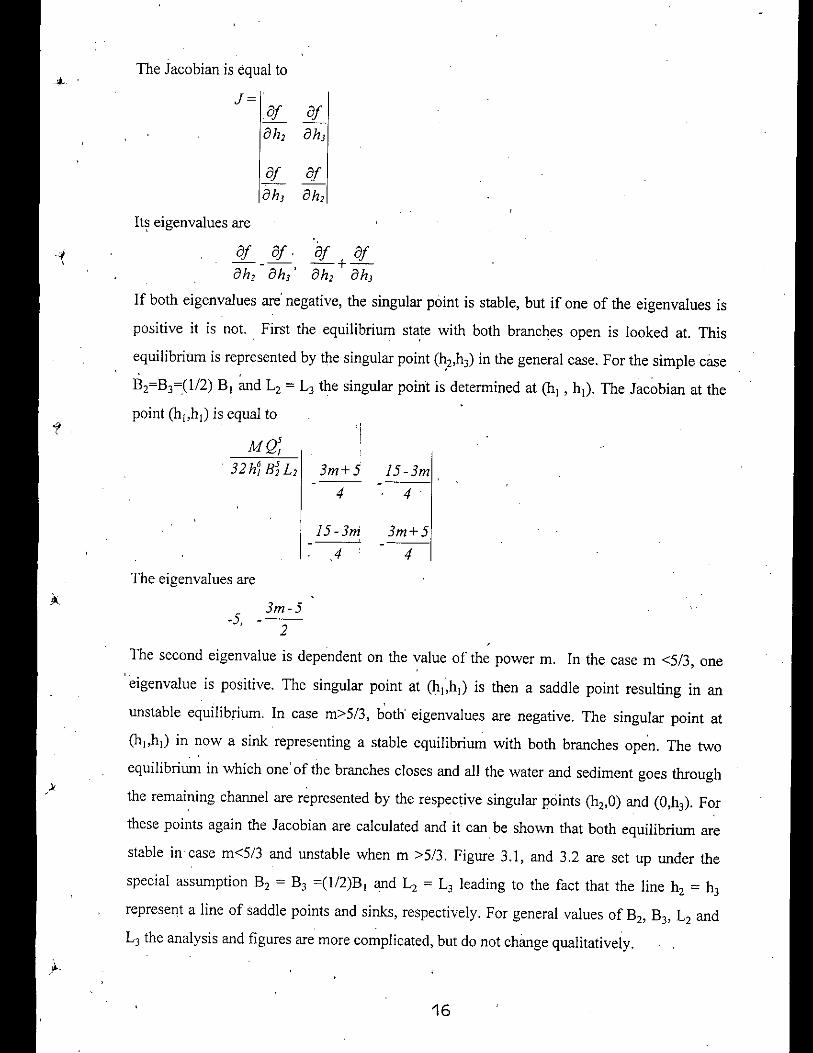
J=

3m+54

15 -3m4

3m+54

15 - 3ni4

af 8f-+-ah, ah,

3m-5-5 ---, 2

If both eigenvalues are' negative, the singular point is stable, but if one of the eigenvalues is

positive it is not. , First the equilibrium state with both branches open is looked at. This

equilibriilm is represented by the singular point (~2,h3)in the general case, For the simple case

B2=B3=(1/2) BI ~d L2 = L3 the singular point is determined at (hI , hi)' The Jacobian at the

point (hJ,hl) is equal to

MQ;32hjBjL,

The eigenvalues are

afah,

The second eigenvalue is dependent on the value of the power m, In the case m <5/3, one

eigenvalue is positive. The singular point at (hJ,h)) is then a saddle point resulting in an

unstable equilibrium. In case m>5/3, both' eigenvalues are negative. The singular point at

(hJ,hl) in now a sink representing a stable equilibrium with both branches open. The two

equilibrium in which one' of the branches closes and all the water and sediment goes through

the remaining channel are represented by the respective singular points (h2'O) and (O,h3). For

these points again the Jacobian are calculated and it can be shown that both equilibrium are

stable incase m<5/3 and unstable when m >513, Figure 3.1, and 3.2 are set up under the

special assumption B2 = B3 =(1/2)B I and L2 = L3 leading to the fact that the line h2 = h3represent a line of saddle points and sinks, respectively, For general values of B2, B3, L2 and

L3 the analysis and figures are more complicated, but do not change qualitatively.

16

It~ eigenvalues are

8f 8f[ah, ah,

The Jacobian is equal to

The above are all for the special case in which the widths and the lengths of the two channels

were exactly the same, as was the bottom roughness. For general values of B2> B3, L2 and L3

the analysis imd figures are more complicated but the do not change qualitatively. Now it is,required to prove that they do not change qualitatively.

the general case may be thought of as a deformation of the symmetric case. For a given

channel network, start out with a symmetric situation and slowly deform the channels until it

reaches the situation as given. During the deformation there are no abrupt changes in the

equilibrium positions. There are three equilibrium, two of which are trivial. If an equilibrium

is stable in the symmetric case, it is stable in the given geometry as well.

This deformation idea can be made precise mathematically. Again' we compute the singular

points. The quotient now'must be

h2 = (i2)5(h2)512(:k. 3)' = (B2)5(L3)512(h2)512(B3)'h3 P 3 h3 B2 B3 L2 h3 B2,

B2)(L3)512(h2)512 '= (~)(h2)712(L3)512B3 L2 h3 a 3 h3 L2

There are two trivial solutions, for which one of the depths is zero, and there is one non"trivial,solution. The differential equation. has three singular points regardless the choice of the

parameters B, L, h. This means that there are no abrupt changes when the geometry of the

channels is defonned, i.e. when the parameters .8, L, h change, stable eq1lilibriu..mremain.stable, unstable equilibrium remain unstable. So, the general case is qualitatively the same as

the symmetric case.

So, it can be seen from the analysis that there are three possible equilibriums. Two equilibrium

situation in which one of the downstream branches is closed and one equilibrium state in

which both the branches are open. It is also clear that tlie value m of the nodal point relation

plays an important role in creating stable and unstable conditions. When m<5/3 the situation

with two branches open is unstable and only a small disturbance is enough to close one of the

branches. When m>5/3 the system always stabilise with two branches open.

17

CHAPTER-4

EXPERIMENTAL SET-UP

The experimental model described herein was constructed on the sand bed in the

hydraulic laboratory of the Water Resources Engineering Department of the Bangladesh

University of Engineering and Technology, Dhaka, during the period of July 1993 to July.

1994. The idea of having the bifurcation set-up was initiated by Prof. M. Vries of Delft

University of Technology with the intention to understand the physics of the phenomena

of sediment transport at bifurcation. The detail of the experimental set-up as well as the .

. measuring techniques are described in the following. articles. General layout plan of the

set-up is shown in Fig. 4.1

" I

4.1 EXPERIMENTAL SET-UP

The experimental set-up consists of two. separate parts, a temporary part and a permanent

part. The permanent part is the experimental facility necessary for the storage and

regulation of the water circulating through the model and the guidance part, The

temporary part contains the actual experimental mobile-bed model of a bifurcation in a

river. It is possible to change the' configuration of this part as and when needed for

carrying out further research on bifurc~tion, using the permanent part of the model

without any drastic constructive changes. The temporary and the permanent part of the

model are shown in Fig. 4.2.

4.1.1 THE TEMPORARY PART

The model of the bifurcated river is built in the temporary part of the set-up. It is a

mobile-bed model with fixed banks. The layout of the channel comprises of a main

branch (denoted as branch 1) which bifurcates into two separate branches, branch 2 and

branch 3. Branches 2 and 3 have different widths. A sediment trap is situated at the end of

each of these two branches, followed by a tail gate for the control of water levels. A detail

)

each of these two branches, followed by a tail gate for the control of water levels. A detail

drawing of the temporary part is shown in Fig. 4.3. In the following sections all elements

of the temporary part are described in detail.

4.1.1.1 INFLOW ZONE

An inflow section and an inflow branch of considerable length are needed to insure equal

distribution of sediment transport, and stable flow conditions before the water reaches the

bifurcation. Water flows from the upstream reservoir to branch I (the main branch) via

the inflow section. PVC tubes (D=2.7 em; L=30 em) are placed over the width of the

entrance to get rid of the larger eddies present in the water coming from the upstream

reservoir and thus the flow is stabilized (Fig. 4.4 and Plate 4.1 ). Immediately after the

arrangement of such flow stabilizing tubes a sandfeeder distributes sand over the width of

the channel . The distributioJ of sand over the width of the channel is done by a wooden, .1

structure which is shown in Plate 4.2.,

4.1.1.2 THE CHARACTERISTICS OF THE MAIN BRANCH

Length (L1) : Before the waterreaches the bifurcation, the sediment from the sandfeeders

should be well-distributed over the width of the branch in a stable flowing conditions.

From experimental experience it is known that a minimum adaptation length L1 ~ 40xh

.(where h is the water depth) is needed to meet this requirement of sediment distribution.

Expected water depth in branch I is chosen to be 10 em which leads to the channel

adaptation length L1 ~ 4.0 m. To make room for the tubes and the supports of the

sandfeeder the branch is made a little longer: L1=4.55 m ( Fig. 4.4 ).

Width (B1): From experimental experience it is known that B ~5xh have the condition of. ,disregarding the influence of the walls. Based on this branch 1 is 1 m wide.

19

4.1.1.3 THE CHARACTERISTICS OF BRANCH 2AND 3

At the bifurcation branch I splits into branches 2 and 3. The radius, length and width of

these curved branches are given below (Fig 4.5).

, Width (B) , Branch I which is' I m in width splits into branch 2 & 3 having an width of

b.4 and 0.6 m respectively.

Radius (R) : To minimize secondary flow inthe bends of these branches the radius R was

selected on the basi~ of criteria R ~5x B and as per discussion with Prof. M. de Vries.

Based on that the values are R2=23.5 m and R)=25.5 m.

Length (L) : The length ofth~ two d'ownstream branches are L2=8.6 m and L3=8.4 m."

-4.1.1.4 CONFIGURATION OF THE BIFURCATION

, The distribution of the sediment transport rate to the downstream branches is governed by, ,

th'e local floW pattern at the bifurcation. From here i~ is seen that the geometry of the

bifurcation plays an important role in this distribution. Therefore the "tip" or "nose" of

, the bifurcation is implemented as a flexible component of the model. The entire model is

made' of brickwork and the nose is made of wood. Three different shapes of noses were

constructed for the this set-up which are shown in Fig. 4.6.

4.1.1.5 SANDTRAPS,

The sandtraps are located at the end of branch 2 and branch 3. The sandtraps intercept all

, the sediment transported through the branches. They 'also prevent the sand to enter into

the permanent part of the model.

The length Ls' of the sand traps is governed by the following equation:

20

The maximum flow velocity in the ,model is determined by the criterion for which only

bed-load transport occurs:

(4.1 )

(4.2)

(4.3)

(4.5)

(4.6)

h W1,. U

=

U. 1-<W-

cU=U.-;g

CUm", =W ;g

C hm",1.,= ;g

,

= flow velocitY;I,

= shear velocity;,u.

u

21

with

Where

C = Ch6zy-coefficient;

W= fall velocity;

This results in an expression for the maximum flow velocity:,

Combining Eq.(4.1) with Eq. (4.4) yields:

The maximum water depth occurs in the C:lse that branch 3 is closed to siltation. In that

case branch 2 conveys all the water, and from Eq. (4.6) it follows that:

;'

22

4.1.1.6 OUTFLOW SECTION

(4.7). - ,-, ,) '-,.fll -V • .(..1ffl

= (BII~B,)

I. Sand trap 2 (corresponding to branch 2): Vs2=0.63m3;

2. Sand trap 3 (corresponding to branch 3): Vs3=0.72m3., ,

The resulting length of the sand traps are (with C=30 m'/2/s): Ls=2.0 m. The sandtraps do

not have a constant width. The widths of the sand traps increase gradually. At the

upstream end they have the width (0.4 and 0.6 m) of the corresponding branch and at the,

downstream end they have the width of tail gate (Bs=I.O m ), Fig. 4.7. The storage

capacity of the sand traps is determined by their length, width and depth,. The available

depth for storage in the sand trap depends on the bed level immediately upstream of the

sand trap. The minimum available depth occurs when the bed level is at its lowest level.i!

Th<:ininimum storage capaciiies of the sand traps are,

a) They regulate the water level in the branch, and

b) They prevent the ~and bed from running dry if a power failure occurs during

experimentation or when it becomes necessary to stop the run for some reason (Fig.

4.8 and Plate 4.3 ).

At the downstream end of the model, the water in each branch flows over a tail gate into

the permanent part of the model. The discharge is measured before spilling into the

downstream reservoir. The tail gates have two functions,

4.1.2 THE PERMANENTPART.'

The permanent part is the hardware 'of the set-up. It acts aS8 facility to conduct all

different types of experiment in the sand bed. The components of the permanent part aregiven below:

.1. Downstream Reservoir

II. Pump

III. Pipe line,

IV. Upstream Reservoir

V. The Regulating arid Measuring System

The components of the permanent part are described below in brief.,

4.1.2.1 DOWNSTREAMRESERVOIR

The doWnstream reservoir (I'!g. 4.9 ) serves as storage reservoir. The volume is II.5m3•

The maximum water level C.ln be at 6.77 m elevation with respect to reservoir bottom.

There is a spillway at the end of the downstream reservoir for excess water to spill out. In

everyone or two weeks the tank had to be cleaned and emptied. The fine particles of the

sediment that are deposited at the bottom are removed through a valve placed at the

lowest level of overflowing spillway.

4.1.2.2 PUMP

The circulating pump near the measuring flume draw water from the downstream.

reservoir. The pump has a maximum delivery of up to 90 Usec and head of 7 m .

.4.1.2.3 PIPE LINE

The lay-out ofthe pipe line is shown in Fig. 4.10. The pipeline has three parts.

(I) Suction pipe line

(2) Delivery pipe line and

(3) Excess discharge pipe line

23

":'

The rate of water flow is taken care of by the pipe line system. The pump sucks the water

from the downstream reservoir irito the pipe line. The T-joint on top of the pump divides

the water over the excess pipe and the delivery or supply pipe, depending on the

regulation of the valves in the respective pipes. As the pump delivers a constant

discharge, the required discharge through the model must be regulated by these valves.

(I) Suction pipe line: It draws water from the downstream reservoir to the pump. It is

1.63m long and the dia of the pipe is a.2m. The suction pipe line is made up by three

pipes. The mouth of the suction pipe is placed .2 m above the floor of the downstream

reservoir (Fig. 4.11 a).

(2) Delivery pipe 'line: The purpose of delivery pipe line is to deliver water from the

pump to the upstream reserv~ir: The length of the delivery pipe is 14.27m and dia of theIi

pipe is a.2m. It has a valve to control water discharge through the model.

(3) Excess discharge pipe line: Its purpose is to discharge the excess water into the

downstream reservoir with the help of the valve which controls the excess water

discharge amount. It is 9.61m long and of dia a.2m.

So, the pipe line consists of three parts. The flow in the channel is controlled with the

help of two valves, one in the delivery pipe and another in the excess discharge pipe.

When more discharge is required in the channel the valve in the delivery pipe line had to

be opened and the other valve has to be closed accordingly. In this way flow of water is

controlled in the channel. The detail of the pipe line are shown in Fig. 4: 12 and Fig. 4.13.

4.1.2.4 UPSTREAM RESERVOIR

The pump draws water from the downstream reservoir and discharge into this reservoir

through the pipe line system. The volume of the upstream reservoir is 4.8 rn3. The

maximum v,:ater depth in the upstream reservoir can be 1.25 m. It has two' chamber one

big and the other is small. Water is dropped into the small chamber of the reservoir from

the delivery pipe line. The main purpose of making the small chamber is to dampen the

24

the following:

The Tail Gates

the delivery pipe line. The main purpose of making the small chamber is to dampen the

turbulence in the water. This small chamber is separated by a wall (with a number of

opening in it) from the large chamber of the upstream reservoir (Fig. 4.14). This is done

to create a smooth inflow into the. big chamber. As undisturbed water is wanted in' the

channel a number of plastic pipes are placed in such a way that water ~asses through

them before going into the main channel (Fig. 4.4). In this way the disturbance w,as

removed. For maintenance purpose the upstream reservoir can be emptied through a

small regulated opening placed at the lower level of the reservoir wall. This also acts as aI, •

storage reservoir.

4.1.2.5 THE REGULATING AND MEASURING SYSTEM

The regulating and measurink system (Fig. 4.15 and Fig. 4.16) of the model consists ofI,,

The stilling Basin Am! Transition Flumes

The Guiding Vanes And Tubes,

The Approach Channel And The Rehbock Weir

The Stilling Basins Connected With Rehbock Weirs

4.1.2.5.1 THE TAIL GATES

At the dis end of the sandtrap of each bifurcated channels the tail gates are placed. The

detail of the tail gates are shown in Fig. 4.8 and Plate 4.3. It is made of cast iron and

encircled with rubber flaps, so that water flows only over the gates. It also has steel'plates

, on both sides for guidance of flow. Ventilation tubes are provided under both tailgates .•

The ventilating tube has a valve at the middle of the tube so that if water gets inside the

.tube it can be drained out. The dis regulation is performed by the tailgates. The flow over

the tan gate is expressed by the following equation.

25

26

4.1.2.5.3 THE GUIDING VANES AND TUBES

(4.8)2"~'q=mB-H -gH.33

4.1;2.5.4 THE ApPROACH CHANNEL AND THE REHBOCK WEIR

To ensure a more smooth flow towards the Approach channels guiding vanes are placed

between the transition flumes and the approach chanp.els which are at right angle to each

other as shown in Fig. 4.16. These v!!lles guide the water around the corner. In order to

prevent 'creation of extra unwanted turbulence in the approach channels, PVC tubes are

used on both the upstream and downstream side of the guiding vanes.

stilling basins as.wellas the transition flumes help destroy turbulence.

The enlargement of the downstream'width of the, sand traps (LOOm for both sandtraps

although the effective width of a tail gate is approximately 0.9 m due to the rubber flaps)

also has positive consequences for the water height over the tail gates, which can be seen

from the above relation.

Behind the tail gates water falls into a stilling basin. In case of branch 2 the stilling basin

is larger than in case of branch 3. This difference is caused due to the available space. The

water from branch 3 has to f~lIow a more n~ow turn (Fig. 4. I 6). This also holds for the .I

transition. flumes. The flume behind branch 2 is much longer. The width of these': ,

transition flumes is equal to the width of the approach channels which is 0.50 m in both

cases. Besides transporting water to the measuring part of the permanent facility, the, .

4.1.2.5.2 THE STILLING BASIN AND TRANSITION FLUMES

The water flows over the tail gate downstream of the sand trap into the stilling basin

before entering 'the approach channel. The approach channels are 5.27 m and 6.12 m long

and both are .50m wide. The approach channel and Rehbock weir are designed according

•••

buffer (Fig. 4.17 and Plate 4.4).

27

THE STILLING BASINS CONNECTED WITH REHBOCK(1.2.5.5WEIRS

4.2 THE WATER CIRCUIT

The water circuit is a closed system'in which water is recirculated. From the Downstream

Reservoir water is pumped to the Upstream Reservoir through the .2 mdiameter pipeline.

Before water enters into main chaimel it passes through the plastic pipes to remove the

turbulence and ultimately passes through the branch 2 and 3. After that water flows

through the measuring flumes back into the Downstream Reservoir.

For the measurement of the «rater height above the Rehbock weirs two stilling basins are

built along the downstream rJservoir. Due to lack of space it was not possible to contract

them next to the weirs. According to ISO 1975, the water level has to be measured at a

upstream position 3 to 4 tim~s the maximum level above the crest of the weir. Hence at• t , ,

such location in each channel a small hole is made in the floor of the approach channel

through which a pipe line was fixed. This pipe line (d=1.5 m) connects the approach

channel with the stilling basing (Fig. 4.17)., The water levels in the stilling basins are

representatives for the water levels at the Rehbock weirs. In the Stilling basin the water

level is measured with 'a point gauge.

to ISO standards, thus avoiding an extra cumbersome calibration. These standard can be

found in the ISO standard Handbook 16, ISO 1438-1975 (E) an.d ISO 1430/1-1980 (E).

The: approach channel should have a miniiiium length of ten iimt:s the width of the

.channel and must be straight and. must have smooth walls, all these conditions are

fulfilled here. The dimensions for the Rehbock weir can be found from Appel)dix A. In

order to measure the water height above the two Rehbock weirs, two stilling basins are

built and point gages are also installed there. The water spills over the Rehbock weir into

.• the reservoir which was made as large as space permits to maximize. the available

,4.3 SEDIMENT CIRCUIT

During the experiment the sediment will be supplied from the sand feeder into the bed at

a suitable rate to avoid local erosion or deposition at the upstream part of the movable

bed, After passing through the main channel and the two branches the sediment will fall

in the. floor of the sand strap, The sediment accumulated in the two sandstraps will be

.weighed, After weighing the sediment it will be left for a certain period to dry and

subsequently will be transported into the silo of the sediment hopper. This recirculating

procedure will be repeated every time,

4.4 SAND FEEDER

To feed sediment and to maintain an equilibrium state in the main channel a sediment

hopper or sand feeder was i~stalled, A sediment feeder is a mechanical device run by

electrical power which feeds sediment into streams of flow of water at measured rates,

and is used for model studies. of rivers. A details drawing of the sand feeder is given in

Fig, 4.18, It is composed of h rectifier, a varia, a DC motor, a gearbox, a gear plate, a

hopper and a sand bucket. The hopper just holds a large amount of sand within it. There

is a narrow slit at the front base of the hopper through which the sand passes out and,

garhers at the rim of the gear plate. As the sand gathers and grow in amount they finally

falls into the sand bucket at measured rates depending on the rotation speed of the gear

plate. The sediment that is feed by the sediment feeder is the same as that of the channel

bed materia!. The calibriltion curves of the feeders are presented in Fig. 4, 19a & 4.l9b,

The sediment falls from the sediment feeder into the wooden structure which dist~ibute

the sediment uniformly over the main channel width.

4.5 SEDIMENTS

The sediment that is specifically chosen for this experiment was bought from the market.

,Then .it was washed, with water so that there is no dirt in it. Several samples was taken

from the washed and unwashed sand for sieve analysis in order to find the grain size

28

distribution. The grain size distribution of washed and unwashed sand can be seen from

Fig. 4.20.

4.6 THE MEASURING TECHNIQUES

In this section the measurements to be made during experimentation are discussed.

Measurements will have to be made of the parameters describing a bifurcation. One of the

aims of the experiments is to study the distribution of the sediment transport rates at a

bifurcation. For this reason a relation was taken into consideration which is given below:

(4.9)

The unkno~ parameters S2, SJ ,Q2 and QJ have to be measured. The measurement of the

waterlevel and of the bed level are also necessary to be measured.'

The factor m is dependent on the geometry of the bifurcation.: !

The factor k is dependent on the widths and also on the value of m (Chapter-3).

The morphological behaviour of the, branches, as a function of the shape of the

bifurcation, is of great interest. For this reason the bed level in the branches must be

measured.

The measurements of the water at the ends of branches 2 and 3 are necessilry for the

setting of the downstream boundary c~nditions.

'4.6.1 DISCHARGE MEASUREMENTS

The discharge is measured at the Rehbock weirs. The individual discharges of branches 2

and 3 are me,asured with the respective Rehbock weirs. These weirs were made according

to the specifications mentioned in ISO (I975). Details of the Rehbock Dimensions are

29

given in Appendix A. The water level at the crest of the weirs is measured in stilling

basins with point gauges, with an accuracy of 0.05 mm. The zeros of ,the point gauges

were set by fiJ.lingthe two approach channels with water up to the crest level of the weirs ..

The point gauges were then adjusted and in this. way the zeros were fixed. The Rehbock

weirs each can measure the discharge properly up to a discharge of 60 lis, with an

accuracy (in the worst'case) of 1.8%. This is detailed in App~ndixB.

4.6.2 . SEDIMENT TRANSPORT MEASUREMENTS

The sediment transport rates in branches 2 and 3 are determined with the help of the sand

traps located at the end of each branch. These sand traps intercept all sediment,transported through the bran6hes. Once a sand trap is emptied and its content measured,

the average sediment transplrt rate for the preceding branch is computed for the time-

interval observed. This is dohe by dividing the amount of sediment by the time elapsed.

The sand traps do not have to be filled completely. It is strongly recommended not to do

so, since the value for the tate obtained would be insignificant. The shorter the time,interval, the more information is obtained on the sediment transport. The sand traps can

be emptied once the model is put to a standstill. Water is always present in the model., ,

The way of removing sediment from the sand traps is to place stop logs in the slots

directly upstream of the sand traps, siphon out the water, and then scoop out the sediment

by hand (Plate 4.5). The method is time-consuming but still this is ,the method which has

been followed here. After the water. is siphoned out, the sediment is taken out from the

sand trap with the help of buckets. Six buckets were used and they were numbered. For

each bucket a chart was developed for weight Vs water weight (Appendix C). So if

weight of water is known the weight of sediment can be easily known. For measuring the

amount of sand in the sandtraps the following procedure is followed. Buckets filled with

sand and water are compared with buckets filled with only water. In this way the

submerged weight of sand was found out. After that the sediment is spread in a thin layer

.across the floor of the laboratory to let it dry. Drying takes about three days. This weight. ,

is translated into a volume (density of sand ps=2650 kg/mJ, porosity p=40%). It is useless

30

31

4.6.3 WATER LEVEL MEASUREMENTS

,for the time interval chosen. The tra.'l~part m:e will varj continuously, but it is not

possible to measure these variations. The only way to get more detailed information on.i

the change in transport rates is to shorten the time intervals for which the sediment

transport rates are determined.

. to define an accuracy for the sediment transport because the tra.."J.3pc~rate is an average

•be measured with it. As can be seen in Plate 4.6b the stilling basin is completely closed,

i.e. there is no connecting hole from basin to branch. The water is siphoned into the

stilling basin via a Pitot tube mounted on a frame laid "cross the width of the channel.

The pitot tube can be moved to different spots in the channel so that it is possible to

measure the water level at different places near the bifurcation.' This may be necessary if

different shapes of "noses" are applied which each induce different local flow patterns ..It

must be that the pitot tube is merely used as a siphon and not as a measuring device; The

readings are taken with a point gauge in the stilling basin which gives more accurate

reading. The water level reading at four stilling basins are taken at every 30 minutes

intervals during experimentation in order to ensure the correct boundary conditions.

The water level was measured at four places in the modeJ. The 'stilling basins are placed. ,

at the beginning and end of each branch (Fig. 4.2 I). The stilling basins I, III and IV are

fixed stilling basins. They render the water level present in a fixed place of the adjacent

branch, namely the water le~il immediately in front of it. It can be seen from plate 4.6aIi

that water passes through a Hole in a wooden palate fixed in the wall of the branch. This' , .

wooden plate can be moved up and. down to ensure that the seepage hole is always

located between the water level and bed level. Stilling basins III and IV are placed

directly upstream of the sand traps. They are used together with the tail gates to regulate

the stream water level. Stilling basin II, which is located near the bifurcation, is a flexible

stilling basin. The water levels at different places in the '1icinity of the stilling basin can

The water level in'a stilling basin is r"eii5llicd .wi;I-, ii jJ01nt gauge. The zeros of the four

point gauges were set by tilling the branches of the model with water which made a

horizontal ~eference level to which all four gauges were related. The accuracy of the

water level measurements is determined by the accuracy with which t~e zero was set. The

error in h is defined as:

The bed level 'was measured with a point gauge in which a .special pin is used. A square,

plate of 2x2 cm2is fixed to the point of the pin to prevent it from sinking into the sand

bed (Fig: 4.22),. The gauge is mounted on a frame which is laid across the channel on the.

branch walls. The bed level is measured at intervals of 0.5 m, in 39 marked cross-sections

of the three branches (Fig. 4.23). In the main branch the bed level is measured at 10

(4.10)

32

er is the error made in the reading;,

ez is the error ~ade in the setting of the zero;

2sm is the errohn the mean of the ;eadings.

.J2 2 2Eh = Er+C:z+4cr'

ll

where

i ".The point gauges have a Vernier scale, so er=0.05 mm and ez = 0.05 mm.

The'standard deviation in the mean often readings was Sm= 0.03 mm.

As a result the water level can be measured with an accuracy eh = 0.09 mm.

. . ,4.6.4 BED LEVEL MEASUREMENTS

,points at each cross-section. In branches 2 and 3 the bed level was measured at 5 points at

each cross-section. The bed level is measured two times in a run, one before starting- the

pump and the other after stopping the pump. The measuring gauge is placed on a wooden

frame which is laid across the width of the channel at one ofthe'croS's-sections previously

mentioned (Plate 4.7). The gauge can slide on the frame across the width of the channel

in order to make a measurement at the desired point of the cross-section. The frame is

made of wood, which deflects slightly' when placed across the channel. This deflection is

"

with which the bed level is measured. The supporting frame is placed on the walls of thebranches.

4.7 TEST RUNS, '

To check the efficiency of the model some test IllilS were made. The test runs were

carried out with the help of a particular type of seed which was selected from a large

variety of seeds. This particular type of seed moves by rolling along the bed of the, .

channel. This movement of tile seed demonstrates the bed load transport which is desired

in the experiment. At least 2Qtest runs with four different discharges were carried out and' !I

the results as shown in Fig. 41.24show that the model is acceptable..• I'

I

33

CHAPTER-S

EXPERIMENTAL PROCEDURE

First the model was constructed as per requirement of the. objective of the experiment

keeping in mind the flexibility needed in such experimental, set-up t,o carry out further

studies in future. The construction period was nearly one. year. For conducting the

experiment the following pro~edure was followed. Running the experiment and collecting

data required not only a great ~eal of physical work but also a careful observation.

5.1 BEFORE STARTING THE MODEL FOR ,EXPERIMENT THEFOLLOWING TmNGS WERE DONE

STEP} :

Sand of grain size of d.3l=300 ~m was selected from the market and washed with water so

that there is no dirt in it. After that sieve. analysis was done in ord~Tto find t.h~llTHinsi7.e, . ' ••....

distribution. From the lot of the sand ,ten samp!~s were taken at rarldom in order to find the

grain size distribution. The results of the ten samples were very close and with the average

value the grain size distribution curve was drawn (Fig. 4.20).

STEP 2 :

Before running.the rhodel several runs were needed in order to find whether the Engelund-

Hansen equation carl be used for this model. This is required for estimating the amount of

sand that should be fed from the sand feeder during the experiment.

STEP3 :

The efficiency of the sandtraps were tested by running the model several times. This is a

very important item. The main purpose of the experiment was to know the amount of the

sediment being transported in branch 2 and 3. If considerable amount of sediment passes

o,ier the two tailgates t'1en it is not possible to know correctly, how much sand actually, ,,passes through the two branches. It hilS been seen that if the discharge is less than 45 Vsec

through each branch of about, 4% sediment passover the tailgate. The data below will give aclear idea about this statement.

STEP 4

All the items such as stilling basms; hook gauges, point gauges, tail gates, stop locks and

other items Were checked whether they were working well and whethe~ these were in theright place of the model.

,STEPS

A method is developed for relating all water level and bed level measurements to a specific

reference level. First the model 'will be filled with water to a certain arbitrary level (z)

above the laboratory floor. In case of no water movement this should provide a perfectly

horizontal reference level. This reference level will be measured with the equipment which

will be used for measuring water levels and bed levels during the experiments. There is no

need to adjustthe zero's of the measuring instruments to this arbitrary reference level. For

each measuring instrument a reading (r) will be obtained corresponding to a water level or

. ,

35

).

,~

bed level, having an elevation ofz meters above the laboratory floor. For any other reading

, (reDthe elevation of the water or bed level above the laboratory floor can be computed using. ,

Eq. given below

elev.= Z - r+rd

STEP 6 :

Calibrating the instruments :

(1) Sand feeder, The sandfeeders have different speeds. At different speeds the rate of

sand outflow was measured td a caljbration curve was developed, For each speed three

measurement was carried out 10 make the calibration curve more accurate. The calibration

curves of the two'sandfeeders were given in Fig. 4.19.

(2) Discharge of water will be measured by two Rehbock weirs. The calibration chart of

the tWoRehbock weirs was made by a standard equation. For detail see appendix A.

, .,

(3) Two valves in the pipe line was calibrated in order to attain desired discharge for a

particular rUn.

, 5.2 DURING, THE EXPERIMENT THE FOLLOWING THINGS WEREDONE:

In order to have good experiments proper handling of both the temporary and permanent

part of the model is required. After the construction of the model considerable time was

spent in order to get knowledge how to run the model properly. A sort of manual has been

resulted from both the knowledge gathe{ed from running the present model as well as with

the advice and remarks from experienced people in this field.

In a particular run of certain discharge for a particular shape of nose or tip, the following

steps have been followed.

36

STEP ONE :

The first step is the fixation of the discharge. Both the excess and the supply pipe line have

valves for the regulation of the discharge. A valve influences the flow rate by changing the

flow area locally. It.is done by the vertical movement of a round steel plate inside the valve.

A wheel on top of the valve is turned to determine the vertical position of tpe steel plate.

Before starting the purnp the valves in the excess and the qelivery pipe line should be

closed. Sufficient depth of water in the downstream reservoir should be present before

. starting the pump. After that by adjusting both the valves, the desired flow rate through the

model was achieved. When the desired discharged was achieved the key from both theI .

valves were removed so that n\Jbody can tum the keys anymore.

STEP TWO:

After selecting. the discharge the pump should be stopped and the sand feeder should be

checked. Even though the sand feeders were calibrated it should be checked before every

run to check whether they feed sand according to the calibration charts. From the Englund-

Hansen formula, the amount of sand that a certain discharge would carry can be calculated.

From the calibration chart, the speed of the s2.nd.feeder was found '.'lith respect to the

calculated amount of the sand. Then .the sand feeder was checked thTee times, whether at

that speed it drops the desired amount bf sediment. After that the sand feeder was stopped

arid water was allowed to drain out from the temporary part of the model. This was done to

dry the. sand lying on the channel bed.

STEPTHREE:

After completing the above two steps the next step was to siphon water from the two sand

traps. This was done by the help of two one inch dia rubber pipes. The siphoning process. ,normally takes 3 to 4 hours.

STEP FOUR :

aefore doing an experiment on the model of bifurcation it is very important to prepare the

bed. The bed preparation has always been done after fixing the discharge, because in this

37

way, the prepared bed will not be disturbed. If the bed is prepared before fixing the,

discharge, ,the bed may be completely destroyed while adjusting the desired discharge.

Another thing should be' kept in mind that one should not do the experiment with an

, arbitrary bed, because more than ten rUns were given with arbitrary bed in which six runs

gave tlldesired results. In that six runs sediment was transported only in one branch, but the

goal of the experiment is to find both S2 and S3' So it is advised, not to work with any"

arbitrary bed level because in that case, one may lose valuable time with no desired re,suIts.

So, before doing experiment with the model, it is necessary to have some idea of the

normal depths of th~ branche~ for a certain discharge. In fact it is impossible to predict the

normal depths because of the' fact that at this time the distribution of sediment in the two

downstream branches of a bifurcation is not known. A method has beel) developed by, '! ,which one can guess the normal depths by taking some assumed value of ni and k, since

normal depths has very little dfect by the variation of m and k. This method is much better

, ,because at least one has som~ idea about what will happen in the model. These calculatedi

depths should be provided in the model. The normal depths were calculate,d by using the. I .

following eight equations:

).

Where,

h = Q 8 (-115) B (-4/5) M(1I5)2 2' ,2 • 2 •

h =' Q 8 (-115) B (-4/5) M{1I5)J J' J . J .

. =Q (-1) 8 (J/5) B (215)'M(-J/5) C(-2)12, 2 • 2 • 2' •

. - Q (-I) 8 (J/5) B (2/5) M(-3/5) C(-2)IJ - 3 • J • 3' •

QI =Q2 +Q3

8( = 82 + 83

i2.L2 = iJ.LJ

82/8J = k. (Q2/Q3t

M = M as used in the sand -transport formula S =BM.un

C = Chezy value

B = Width of the channel branch

38

•

(5.1)

(5.2)

(5.3)

(5.4)

(5.5)

(5.6)

(5.7)

(5.8)

First the upstream discharge was chosen and then the ratio Q~/Q3was chosen. From QZ/Q3. I . ,

and Q, the value of Qz and Q3 was found. Than by solving eight equations simultaneously

the normal depths in the three branches were found. A program' has been developed in

QBASIC to find ,the normal depths by solving the eight equations simultaneously

(Appendix D). This method also helps in checking whether the velocities in the ,branches

dominate only bed load transport or not. It has been found that if the velocity in all the

branches are more than .22 m/sec, then for dso=.027 mm the bed 'load transport

predominates. When the normal depths of the branches has been found the next thing is to

cal~ulate the d~pths of bed fot all 39 sections. Now from the calculated depth, at differentI

sections; the bed was preparetl. During the preparation of the bed the sediment should be

dry enough otherwise, it is nbt possible to prepare the desired bed level. For that reason

after draining water from the channels at least 10-15 hours time should be, given to let the

sediment in the channel to dry. When preparing the bed the depth of water in the upstream

reservoir should not be greater than 0.7 m otherwise water will enter into the main channel. .

STEPS

After preparing ,the bed the tail gates were lifted to its maximum position. This is done

because, the next thing is to fill the temporary part of the model with water, so, no water

should be allowed to' pass over the tail gates. '

STEP6 :

Once the bed is prepared, the channels will be filled with water. This step has to be done

very carefully because a slight mistake can damage the prepared bed.By the help of a half

horse power pump both the sandtraps were filled simultaneously upto the concrete floor of

the channels. When. the water level reaches the floor level of the' branches the sandtraps

were filled very slowly so that the bed is not disturbed. First the sand will be wet and after

that water will move slowly towards the nose of the bifurcation. Attention should be paid,

so that water in both the branches moves toward the bifurcation point simultaneously. When

water reaches the nose from both the branches, the upstream reservoir was very slowly

, filled with water, With the plastic pipe, which was connected to a tap near the upstream

39

or less at the same time.

,~,filled with water, with the plastic pipe, which was connected to a tap neat the upstream. ,reservoir. The upstream reservoir should be filled in such a way that when .water coming

from both the sandtraps reaches section- I ,water from upstream reservoir should also reach,section~I. This' filling process continued until the depth of watt<r in the branches reached

. ISm. By this process the disturbance in the bed was removed. In order to develop this

te~hnique which is very important a loi of time was spent.

, STEP 7: , I' . ..,When the channels are filled with water upto .ISm, 2 to 3 hours time have been given for

the water to settle. After that all the water level measuring instruments were checked,, .

whether these were working well with reference to any arbitrary water level. The pitot tube

of stilling basin 2 was checked and also the silo of the sand feeder was checked whether it is

filled with sand or not.

STEPS

Now it is time to take the initial bed level reading. This initial bed level reading should

however. be taken at least 2 to 3 hours after filling channels. The bed level reading was

taken by point gauges. For sections I to 12, 10 readings were taken at each section and for" '

sections 13 to 39, S'readings were taken at each section.

STEP 9,

Now.the pump was, ~tarted and water was allowed to rise in the temporary part of the

model upto .20 m. Care was taken so that the pump and the sand feeder were started more,

STEP 10

When water depth reach near .20 m in the branches the tail gates were opened very slowly

to the desired level. The tail gates should be opened at the same time and with care so that

there is no sudden disturbance in the bed of the branches.

40

,r

STEP 11\ ,

After setting the tail gates to their desired levd the depths Of w~ter in the branches were

checked by the help of four stilling basins; It was also checked whether the sediment

movement occurs in both, the downstream branches. Readings, of the Rehbock weirs were

taken after about 20 min. of running the model and the discharge was checked whether the, .model was running with the desired discharge. If the discharge is not very close to the

desired discharge; the tail gates were lifted and the model ~as stopped. Then the steps I to

II were repeated until the model was found running with desired discharge.

STEP 12 : '

The readings of the stilling basins and the Rehbock weirs were taken at every half an hour.' ,

and quarter hour intervals, respectively. The first readings were taken after half an hour of

running the model.

STEP 13 :

After completing the eleven steps the model was allowed to n,m for 8 to 10 hours and data

wascollected as per step 12. From practice, it was seen tha~ by this time good amount of, .sediment stores in the sand traps.

STEP 14 :

After running the model for about 8 to 10 hours, the tail gates were raised simultaneously to

their maximum position very slowly and then the pump was stopped. The tail gates were

raised ,;ery slowly so that there was no disturbance in the char1nel beds. The sand feeder

was also stopped at the same time.

STEP 15 :

When the model was stopped\ about 2 to 3 hours time was given for the water lev~1 to,settle. Then the bed level reading was taken. This was done in the same process as before. .(step 8) and that gave the final bed level reading.

41

42

STEP IT

.CONSTRUCTION,

STEP 18 :

,After the bed level readings were taken the stop locks were placed in its position. After

plaCing the stop locks,' two rubber tubes were placed between' the stop locks" and the

concrete walls."Then the tubes were air pumped by a pumper so that no water or sediment,passes through the 'stop locks. This was done because the main purpose was to measure the

sediment in the sand traps.

When the stop locks are water tight water from the sand traps were siphoned by the help of

two plastic pipes. Care was taken so that no sediment was siphoned out. After the water was

siphoned out from the sand traps the sediment was collected and weighed. This was the

amount of sediment that passed through the two channels for that particular runtime.

STEP 16':

After weighing the sediment from the sand traps the sand was allowed to dry for several

days and'then they were ready for the next run.

i) Instrument Fabrications :

In designing the'Rehbock weirs, Guidevanes, Tailgates and Stoplocks various kinds of

problems were faced. It was very difficult to build them according to the ISO specification

because of scarcity of required materials and inadequacy of experience in such field.

1.. DURING CONSTRUCTION OF THE MODEL

,S.3 PROBLEMS FACED DURING MODELOBSERVATION AND DATA COLLECTION

'ii) .Civil Work :

It is' obvious that skilled mAson .will not be available. Normally the masons are all

experienced in constructing buildings and other structures where aq;uracy is not so much

important. They are not expelienced in constructing a physical model where in some places

accuracy of less than' 0.5 % is required. So, due to this the construction of the model took a' ,

long time. Also it was seen that the model was not water tight,in many places. To make the

model water tight a considerable amount of time was spent.

iii) Inaccurate Measurements :,

Duling constructing .of the model VaJ10USproblems were faced with many components

made of steel. Initially a lot errors were made while constructing these components in the

workshops. So, it was decided that a prototype of exactly s~e size of all steel structures

will be prepared with cartoon paper and then it was supplied to the workshop for

construction. This process also took much of the time but the result was very good.

2. PROBLEMS AROSE DURING CALIBRATING THE SANDFEEDER :

i) Duling the. time. of construction of the model attempts were taken to cfllibrate the

sandfeeders. Sandfeeders were lying in the laboratory for a long time and needed substantial ', ,

repair work, before calibrations. So, both the sandfeeders were sent to the workshop for

repair work that also took a long time., ,

Ii) When the sandfeeders were, ready, they were tested and it was seen that at a particular

speed the sandfeeders were giving different outp4ts. Soon.it was realized that this problem

was due to the different ~oisture contents of the sand. To get lid of this problem the sand

was dlied and kept in a particular storillg place constructed within the laboratory. This gave

, good results.

3. PROBLEMS WITH THE SAND

The problem with the sand i'as that it contains a large amount of dirt. At the beginning

. several runs were carried out with un-washed sand. The problem with unwashed sand was

that the bed and the sandtraps could not be seen clearly. There were also problems with

Rehbock weirs because of the facts that a large amount of dirt was passing over the

43

permanent part a'ld small holes were' clogged ".•.ith dirt. So, after running the model for five

to six hours, the stilling basins, readings of the Rehbock weirs were different from the initial

readings. Another problem is that after every run the whole model has to be cleaned which

is a very difficult and time-consuming task. It was tried to see how the running of the.model

with unwashed sand will help to rem~ve the dirt. It was observed that this process will

takes' much longer time than washing at first. To overcome these difficulties it was decided

, that first the sand will be washed and then it will be used.

4. PUMP:

i) The problem with the pump was that it was not running according to its specification.

The discharge was not more than 25 Usec even though as per specification' it should have

been much more. So, the pump was tested in the laboratory of the Mechanical Engg.

Department and was found not suitable. So, after detail calculation taking into account the

present and future research requirement a pump of90 Usec capacity was purchased.

ii) ,.The next problem with the pump was when it was sucking water, due to less depth of

wat~r (.77m) in the downstream reservoir, a vortex was created. The vortex made a big

fluctuation in the discharge due to time to time air sucking through this vortex. In order to, "

get rid of such vortex some wooden' frames were placed on the water surface as a easier,

solution. This did not improve the situation substantially. Hence a portion of the

downstream floor (1.5 x 1.5 m2) was lowered by 1.5 m to give sufficient submergence of

suction pipe of the pump (Fig. 4. I la). This gave good results.

5, PIPELINE:

If the layout of the pipeline is not proper various kinds of problem may arise. In the model

the first layout of the pipeli~e (Fig. 5.1) was not proper and this resulted in negative

pressure at certain location of the pipe line. This also created too much disturbance in the

upstream reservoir when the water drops from the pipe ,line. So, it was decided to lower the

layout of the pipeline. The pipe line was then lowered and this gave good results.

6. WATER:

There was some problem with availability of water. The storage capacity of the downstream

reservoir was constructed as big as possible with the available. storage space keeping in

mind the functioning of various components of the experimental set-up. The storage

capacity thus created was not enough to run the model without adding water from the direct

line atth~ starting of the experiment to fill-up the channels, sandtraps etc. This requirement

of additional quantitY of water from direct line could not be met most of the time. In order

to solve this problem all the storage tanks in the laboratory were checked and it was found

that the storage t~ of the 70 feet flume may be used for this purpose. Accordingly every

day at night the 70 feet flume's reservoir tank was filled with water and later on with the

help of a half horse power pump water was supplied to the model from that tank ( Plate.

5.1). Thus the problem was solved.

7. DISTRIBUTION OF SAND OVER THE WIDTH OF THE CHANNEL:

To ensure proper distribution of sand that is fed from the sandfeeder over the width of the

channel was a difficult task. First attempts were made with a 0.10 m dia. plastic tube. The

plastic tUbe was cut into halves along the length and then on the periphery of one half, holes

were made and then it was placed in an inclined position to distribute the sand across the

width. This process did not serve the purpose properly. After that another attel)1ptwas made

with that plastic pipe but this time the holes were made in such a way that when the half.. .section was placed in an inclined position the smaller holes were at higher elevation and the

bigger ones were at the lower elevation. This improved the distribution of sand over the

width but did not satisfy the requirement. At last a wooden structure was constructed by

trial and error method to help distribute the sand and this gave the desired result (plate 4.2).

45

, '.

CHAPTER-6

DATA .ANALYSIS, RESULTS AND DISCUSSION

, Data on sediment movement and distribution over the two downstreanl branches of a

bifurcation were collected from the laboratory model which was developed for this. , .

'purpose. The intention was to understand the physics of the phenomena of sediment

transport at a bifurcation. The data were collected mainly relating to

(a) Anabranch discharges Qz and Q3'

(b) Anabranch average sediment discharges Sz and S3'

(c) Average water level of all the three branches.

(d) Initial and final bed level readings of a run at all the 39 sections.

These are all described is detail in article 4.6. For the purpose of data collection, two

sets of runs were carried out. In the first set there are 2! ru..'!s a..'!dirr t.~e secorrd set t.h.ere

are 20 runs. The first set is with the reference nose and the second set is with the second

nose.

The. 21 runs with the first nose is divided into three groups. The first group contain 8

runs with discharge around 30 lis. The second and third group, contains 6 and 7 runs

with discharge close to 40 and 20 lis respectively. The 20 runs with nose 2 again were

divided in three groups. The first group contains 9 runs with',discharge 30 I/s. The

second and third group contains 6 and 5 runs with 40 and 20 lis respectively. In all the

runs of a group it was tried to keep the total discharge and the sediment input rate

constant. The main purpose of all the' runs were to study whether the value of m and k.1.

in Eq. 3.5 vary with discharge or not, for a particular nose. Visual obserVations were. .!

made during the period with a view to study the pattern and the process in channel

. bifurcation, evolution and morphology of the bifurcation of model channels.

Photographs were also taken during the run.

. 'I'

6.2 INCIPIENT MOTION

(6.2)

(6.1 )

. .

4-7

uJgU.=-:-

:C

and

6.1 COMPILATION OF DATA

6.2.1 MODE OF TRANSPORT

Froin all the experiments the value of 1:. and R. were calculated and they were found

within the range of .09 to .25 and 86.54 to 195.31 respectively. This shows tlUtt they

were all above the Shields curve( Fig. 2.4 ). So, it can be said that in the present study

flow range were sufficient to make sediment in motion.

, .To check wh.ether the transports are bed load or not. For all the runs, .U./W was

calculated and they were found less than 1 which indicates that all the transport in all

the branches of all the runs were moved as bed load.

Here

The present research was aimed to understand the physics of the phenomena of sediment

transport at a' bifurcation and to try' to develop an empirical 'relation to calculate

sediment transport rate in the two downstream channels at, bifurcation. To do this a

, nodal point relation was assumed (Article-3.1) in which there were. two constants m and

k. Accordingly laboratory experiments were carried out for different sets of conditions.

A total of 41 runs were conducted. The bed level evolution at different sections of all the

runs or'the three branches are shown in Fig. 6.1-6.41. Fig: 6.1-6:21 is for the first nose

and Fig. 6.22-6.41 are for the second nose. The variation of discharges with run time of

, all the three branches of the 41 runs are shown in Fig. 6.42-6.47. Fig. 6.42-6.44 are for

the first nose and 6.45-6.47 is for the second nose. In the following articles detail

discussion on observation and results are made.

j,

6.3 BED LEVEL EVOLUTION

The bed level evolutiop of the three branches of all the runs are shown in Fig. 6.1 - 6.41:

As it was mentioned in Chapter-5 that before starting the model for a particular run the

bed wasp'repared with 'the normal depths. These calculated normal depths are not the

accurate depths because here the value of m and k are assumed aild it is still not known

how the sediment will be distributed at a bifurcation. This method is used just to get an

idea whether the model normal depths are near the ,calculated depths or not and also to

save time so that there is no run in which szls) is very large or zero. Run NO.2 is an

example where s2/s) is negative in value. So, this run can not be used since unrealistic

result occurred. The problem with Run NO.2, was that in branch 2 bed level was 25

cm lower and branch 3 was 15 cm higher than the normal depths respectively, so all the

sediment went through branch 2 because it was lower than the normal depths at the

beginning. 'Branch 3 at the beginning had a lot of sand in it. So, from this it is learnt that

one should not deviate much from the normal depths otherwise undesired result may

occur. It should be noticed that in all the fW1S branch; had the least change (Table 6.1

to 6.6 ) of bed level because it is upstream of the bifurcation point. The main objective

, was to keep the main branch (I ) more, or less in equilibrium and to. pass as much as

possible the amount of sediment that is being supplied by the sandfeeder. In all the runs

more or less it was achieved. For the first nose except Run No.2, in all the runs one of

the two downstream branches were kept only a few cm higher than normal depth and

other was a few cm lower than normal depths. In all the runs of nose I it can be seen that

deposition occurred in the branch which was lower than the normal depths, and scouring

or' erosion occurred in the branch which was higher than the ~orrhal depths. So, from

this it can be said that the assumpted nomal depths were not very far from actualI

normal depths.

In case of second nose it can be seen 'that the normal depths relation was no longer,

helpful. In all the run of Nose 2 it can be seen from Fig. 6.22-6.41 that the bed level of

branch 2 was getting higher and higher and most of sediment that was fed by the sand

feeder was being ,carried by branch 3. This behaviour was different from nose-I and the

calculatea normal depths were completely different. The reason behind this is, in the

first nose .the ratio of the widths of the two branches at the nose was the sameo! the ratio

48

. Run NO.1 to 8 were with 30 IIsec. In Run No. I branch 2 was higher than calculated

normal depths and branch 3 was kept lower than the normal depths. It was observed in

this run that there i'sdeposition in branch 3 and erosion in branch 2. In Run NO.2 branch

2 , was lowered and branch 3 Iwas kept quite high. In this run almost all the discharge"and sediinent wen~ through th6 smaller branch. From observation of these two runs itI .

was concluded that this type of run will not give required result. So, in all the runs from

3-7 the channel bed was fixed jn such a way that depth of flow was more or less same asI

6. 3.1 RUNS WITHTHE FIRST NOSE ( BED LEVEL EVOLUTiON)

49I

the calculated depths. All these runs gave realistic data. After completing 7 runs, data

obtained from six runs neglecting Run NO.2 were used and the value of m and k were/' : .

comP'lted. With results so obtained the bed of Run No 8 was prepared and experiment

was carried out. From Fig. 6.8, it can be seen that there is no change in bed levels in all

the three branches. In Run NO.8 at the beginning of experiment the average depths in

branches 2 and 3 were 261.5 and 263.13 mm and at the end they were almost the same.

So, it can be inferred that the equation of nodal point well fits with the situation.

,first.nose the ratio of the widths of the two branches at the nose was the same of the ratio

of widths of the two downstream branches but for the case of the second nose it was not.

Due to this an additional disturbance was there. In order to encounter this sit)lation there

should be some change in the nodal point relation or the branches widths should be 20

and 80 cm respectively of branch 2 and 3. So, the bed level changes due to nose-I can

not be compared with those due to nose-2 since the situatio,n are different. Also in

branch I of all the runs except for the 20 lis runs section I-I at the end of the run, goes

far below from the initial position. Section I-I is just 0.8 m below the point where water

enters into the model from upstream reservoir and just 0.5 m below the section where

sand was falling into the model. When water enters into the model from the upstream

reservoir in case of 30 and 40 lis ,due to initial disturbance the bed level goes down in

section I-I. Also it has been seen that section 1-1 goes down to a certain point for a

particular run and after that it does not go down any more. This can be seen in run no 3,

4,6,7 and 8.

, c

"

Run 9 to 14 were with 40 Usee. In Run NO.9 branch 2 was,kept much higher than, ,

normal depth and branch 3 was kept much lower than normal depth. In this run it was

seen that bran~h 2 was eroded and branch 3 deposited, In run 10 and II the bed levels'

were kept more or less near the calculated normal depths, It can be seen that there were

less changes of bed level ( Table 6.2 ). In Run No. 12 branch 2 was made lower and

branch 3 was higher than the calculated depths which was just the opposite of run no. 9.

Here it can be seen that there was erosion in branch 3 and deposition in branch 2 (Table

6.2). This proves that the actual normal depths are very close to calculated normal

depths. In Run No. 13 and 14 in both the downstream branch, instead of making whole

branch higher or lower then the calculated nonna! depths only same se<;;tionswere made

higher or lower. In these two runs the tot?J hed level cha.!lge in volume. of the two

branches were not much but the sudden ups and downs in some sections caused

irregular final bed level.

Run no 15 to 21 were carried out with 20 Usee. Run No. 15-19 were carried out in the

same process as before ( earlier runs) and the similar results were observed. Relating to

runs with 20 l/s, it may be mentioned that section 1-1 did not go down like the

previous runs with 30 and 40 Us.This is because here the discharge is less and hence the

'disturbance at the inflow zone was small enough not to cause any scour. After

completing the 5 runs (15-19) the value of m and k were determined and the initial bedI '

level of Run No. 20 was preP1rredwith these values. It can be seen from Table 6.3 that" ,

minimum bed level change pccurs and almost all the sand that was being fed were

carried a:way. After that another run was carried out with different QiQ3 ratio to see if

the value of calculated m and k vary much but it did not. So, the calculated .value of m

and k were c<;Jnsideredto be correct for 20 Us discharge.

'6.3.2 RUNS WITH THE SECOND NOSE (BED LEVEJL,EYOLVTION);

Run no 22 to 30 are done for 30 Usee. After running the 22nd run it was seen that it was

not behaving like the previous runs. In this run the bed level of branch 2 was getting

higher with run time and the discharge in this branch was getting lower and lower as the

time goes on. The reverse thing happened in branch 3 but here the bed level was not

'lowered rather little deposition occurred in it (Table 6.4). This result provoked to'

50

;'

'lowered rather little deposition occurred in it (Table 6.4), This result provoked to

continue the same run for longer period, So, Run No, 2~ ,to 26 was carried out as

continuation of Run No, 22. It can be seen from Fig. 6.23 and 6.24 that the bed level of

branch 2 was increasing and the amount of sediment trapped in trap 2 was de~reasing.

On the other hand the sediment in 'trap 3 and also the discharge of branch 3 was

increasing from run to run. In Run No. 25 and 26 it was seen that there was no change is

bed level and discharge. So, the run was stopped and it was decided to continue with a

new prepared bed with different Q/Q3 ratio. Rim No. 27 to ~O was done for this

purpose and siI?ilar evolution in bed level had been observed like Run No. 22 to 26.

So, tills gives all idea that the nodal point reiation was no ionger appropriate for this

situation because there is an extra disturbance due to additional restriction imposed by

the nose. In the same way for 40 and 20 Usec run were carried out is order to see what

happens for the value of m and k.

Run No. 31 to 36 were done with 40 Usec. In this runs 3 I to 33 and 34 to 36 was done

with two different initial bed. In these runs the same thing happened as with the ,runs

with 30 l/sec but here the changes were faster which can be seen from Table 6.5.

Run no 37 to 41 were done with 20 'usec. Here also same this happened. So, all these

runs proved that the effect of, nose 2 are completely different than that of nose I. The

results of nose-2 can possibly~e compared if the widths of branch 2 and 3 are 20 and 80

cm respectively.

6.4 DISCHARGE VARIATION WITH TIME

Discharge variation with run time for all the three branches and for all the runs are

shown in Fig. 6.42 to 6.47. From Fig. 6.42 to Fig. 6.44 it can be observed that there is

very little change of discharge with time in all the three branches of all the runs for the

first nose. It is however observed that in case of the second nose there is a great variation

of discharge with time both in case of branch 2 and 3 even though the total or main

branch, discharge remained the same. This can be seen from Fig. 6.45-6.47. The

following paragraph explains the phenomena with example.

51

52

6.5 PHYSICS OF THE PHENOMENA

more or less constant. On the other hand in case of second nose for run no 22 it can be

seen that at the beginning the discharge in branch 2 and 3 were 8.5 and 20.6 Us• ' I •

respectively. At the end of the 22nd run the discharges in brarich 2 and 3 were 5.07 and

24.31 lis respectively. In all the runs of nose 2 such variation of discharge occurred. In

the discussion of bed-level evolution it was mentioned that bed level of branch 2 was

rising gradually. This rise of bed level caused decrease in discharge. In branch 3 the

opposite phenomena occurred. Run no 22 to 26 was carried out starting from the same

initial bed and the initial discharge. At thy beginning of Run No. 22 the discharge in

branch 2 and 3 was 8.5 and 20.6 respectively. At the end of23rd, 24th and 25th runs the

discharges in branch 2 and 3 were'3.76 and 24.53 lis, 3.26 and 25,18 Us and 3.04 and, ,

, 25.54 Us respectively. At the end of the 26th run the discharge values were almost the

same as at the end of 25th run. Similar phenomena can also be seen in run no 27 to 30,

.31 to 33, 34 to 37, and 37 to 41. In all the cases the discharge in branch 2 decreased and

discharge in branch 3 increased.

In case of the first nose i.e. Run No I to 21 the discharges in all the three branches are, "

It was observed from the experiments with first nose that erosIOn occured in the

downstream branches in whidh the bed level was higher than the normal depths and

deposition occured in the downstream branch in which bed level was lower than normal

level. When the bed level in both the downstream branches were very close to normal

level only small changes occured. However near the circumference of the nose some

erosion occured (approximately 3 cm to 4 cm in depth) due to, disturbance in flow.

From the experiment with the second nose a different phenomena was observed. Here

the bed level of, branch 2 was getting higher and higher irrespective of its initial bed

level. In this case the bed level changes were influenced due to expansion of flow' in the, "

second branch and contraction 'of flow in the third branch immediately below

bifurcation. Here also near the circumference of the nose scour occured (5 cm to 6 cm in

depth). In this case the amount of scour was greater than 'nose I because of more,. disturbance. This phenomena has been explained elaborately in Article 6.3 & 6.4.

:~

.,

6.6 SEDIMENT MEASURED IN SANDTRAPS

The method of measuring the amount of sediment trapped in the sandtraps of branch 2,

and 3 were discussed in detail in article 4.6.2. TIle amount of sediment trapped in sand

trap 2 and 3 can be seen from Table 6.1 to 6.6. From the tables it can be observed that in

case of the first nose or the reference nose each of the sand traps trapped appreciable,amount of sand. But in case of second nose trap 2 collected very little amount of

sediment compared to trap 3. In case of the second nose the amount of sand that was

entering branch 2, most of them were deposited in the branch. The change in volume of

sand of all the b~itnches of all the runs can be seen from Table 6.1 to 6.6.

6.7 ERROR IN DATA ACQUISITION

The main objective of the experiment is to have. some idea of sediment distribution at

bifurcation. In this respect the majn, ratio that are required to express a relation are

CJ2/'lJ and' S/S3' Now it is very essential to know how much accurate these measured

values are.

IN CASE OFO;iQ;>l

!The discharge are measured ~t the two Rehbock weirs and it was found that they are,capable ofn:easuring with arl accuracy of 98.2 %. This is detailed in Appendix B.

IN CASE OF szLs;>l. ,

'The sources of error may c01l1efrom following:

a) The sandfeeder

b) The bed level measurements,

c) The sandtraps, ,

d) The buckets

From the sandfeeder it was seen that due to the machine and the ,difference in moisture

content of sand, maximum amount of sediment measurement errors are around 7%. In

case of bed level measurement the amount of error are 3% due to point gauge reading

53

and accurate bed level detection. During the collection of sand from the sandtraps the

amount of sediment lost is about 6% (maximum). During the time of weighing with. ,buckets the error is around 3% due to the deformed shape of the buckets. So, in total

the error may be to the amount of 19%. But from Table 6.1 to 6.2 it can be seen that

except for Run No. 12 all are with in that range of 19 % tha( means the results may

be considered to be acceptable.

After doing necessary calculation s2/s] and 'h/q, were plotted for both the noses for

different discharges and these are shown in Fig., 6.48 to 6.53. It need to be mentioned

that the ratio of szls] was on the 'basis of average values since they were calculated from

data measured at the beginning and end of the run time. For that reason 'l2/'b ratio was

also calculated on the basis of average value of'l2 and 'b. Fig. 6.48 to 6.50 show how

,szls] varies with 'l2/'b for the first three sets of experiments using nose I for three

different total discharges, 30, 40 and 20 lis respectively. From each figure it is evident

that as 'l2/q] increases szls] also increases. This is obvious due to the fact that as 'l2/'b

increases, 'l2 increases' and '13 decreases resulting in an average trend of increase in S2

and decrease in S]. From the ~lotted points in these figures it is observed that the pointsI

are relatively more scattered in Fig. 6.50 which is for lowest total discharge of 20 lis.

The low discharge is associated with low velocities which in case of 20 lis may be too

lowto cause sediment move~ent properly. Figl1fes 6.51 to 6.53 show variation of $zls]I • _ •

with qzlq] fo~ second three sets of experiments with discharges 30, 40 and 20 lis using

second nose. It is to be mentioned here that in case of second nose the nose

configuration is such that in the second channel flow expands downstream of the n~se,and in the third channel flo~ accelei'ates do",,,,",sti'cu';;:;of the nose. This u'dditional

influence of nose on flow parameter obviously will have additional impacts on sediment

distribution in the two downstream channels as compared to' effect of the 1st nose for

the same discharge ratio.

Results from this set of experiments also shows increasing trend of in szls] ratio with

the increase of'l2/'b ratio as normally expected. It is observed from Fig. 6.51'to 6.53 that. . ,

the plotted points are more scattered in case of experiments with second nose. This

6.8.1 DEVELOPED RELATION BETWEEN SEDIMENT AND FLOW

The general. form of equ~tion have been determined from the best fit lines in Figs. 6.48

to 6.53. The six,different equations corresponding to six different sets of experiments are

given below. '

(6.5)

(6.3)

(6.6)

(6,7)

.(6.4)

(6.8)

55

For Q= 40 lis". . 2.958

sis) =2.411 (~/~)

For the second nose'

For Q= 20 lis2.4928siS3 = 1.25213 (~/~)

F~rthe first nose' '

For Q= 30 lis

~/S3 = 1.39202 (~/~)4.71315

'may be due to the configuration of'the 2nd nose which created additional impact on

flows 'in doWnstream channels or due to the low flow which causes inconsistent

sediment transport or combination of both, Fig. 6.52 shows less scattered data where

the flow is higher compared to other runs. May be in this case the additional impact

due to nose configuration was relatively less.

For Q= 30 lis

S2/s3 = 1.14463 (~/~/,54414

For Q'" 20 lis.. I 19381

sis) = 1.87398 (~/~) ,

'FOr Q= 40 lis ,5.6545

. S2/s3 = 2.0148 (~/~)

"

6.8.2 VALUES OF ill AND k

NOSE 1 NOSE 2DISCHARGE (lis) DISCHARGE (lis)

20 30 40 20 30 40, ,m 2.4928 4.71315 5.6545 1.9381 2.54414 2.958k 1.25213 1.39202 2.0148 1.87398 1.14463 2.411, ,

From the above table it is observed that for both the noses the values ofm increases'with

increase in discharge. This may be due to relatively more increase in velocity in channel

2 for higher CJ2/<J.J ratios for higher discharges. This results in greater increase of '

sediment discharge in channel 2 for higher CJ2/<J.J ratios at higher discharges. From the,

study of m values in equations mentioned before it is observed for equal discharge m

values for the second nose are lower, than the corresponding mvalues for the 1st nose.

This may be due to additional impact on flow in downstream channel due to flow

expansion 'in second channel resulting in rise of bed level in the, earlier part bf

experiment with each CJ2/<J.J value. However it is felt that such a comparison on the effectI

of two different noses need not be attempted with limited data available at this stage.

6.9 SIMULATIONS WITH I-D MODEL (WENDY). ,

From experimental data relations have been obtained for sediment distribution at' ~

bifurcation. These relations are for three different discharges corresponding to each ofi '

, the two different noses used in the experiment. Jhe general form of the relation is as

follows:

, '()'"S2 = k q2

S3 q3

The m and k values have heen found different not only for different noses but also for

different discharges. For the discharge of 30 lis with the first nose the above general

56

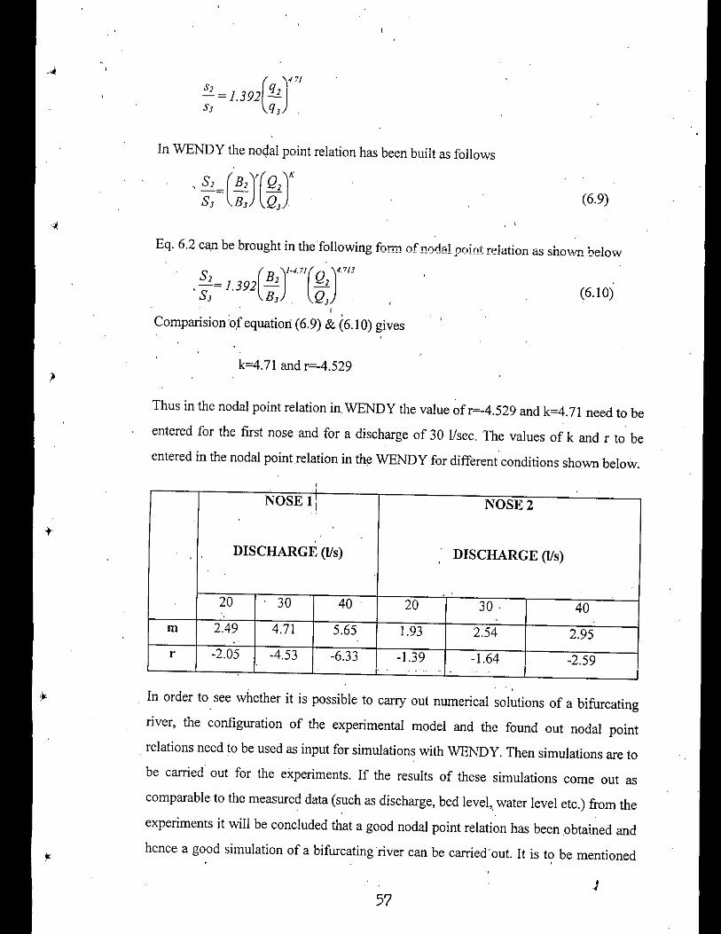
57

(6.9)

(6.10)

Eq. 6.2 can be brought in the following form ofnodRl p(,int relation as ShO"iIl below

In WENDY the no~aI point relation has been built as follows

k=4.71 and r=-4.529

J

( )

471

s2=1.392 q2s] q],

.82= 1.392(B2)/'47Jl/ Q2)".'/J8] B] Q]

I

Comparision :of equation (6.9) & (6.10) gives

Thus in the nodal point relation in,WENDY the value ofr=-4.529 and k=4.71 need to be

entered for the first nose and for a discharge of 30 lIsec. The values of k and r to be

entered in the nodal point relation in the WENDY for different conditions shown below.

NOSE I: NOSE 2

DISCHARGE (lis) DISCHARGE (lis)

20 30 40 20 30. 40m 2.49 4.71 5.65 1.93 2.54 2.95.r -2.05 -4.53 -6.33 -1.39 -1.64 -2.59

.. 1-

In order to see whether it is possible to carry out numerical solutions of a bifurcating

river, the configuration of the experimental model and the found out nodal point

relations need to be used as input for simulations with WENDY. Then simulations are to

be carried out for the experiments. If the results of these simulations come out as

comparable to the measured data (such as discharge, bed level,.water level etc.) from the

experiments it will be concluded that a good nodal point relation has been obtained and

hence a good simulation of a bifurcating river can be carried' out. It is t<;>be mentioned

)

here that the nodal point relations which have been worked out will be valuable only for

the specific conditions of the experiment. The ultimate goal is however to get a relation

which can be used in all circumstances, Hence much more research are to be carried out

to reach the ultimate goal.

6.10 SOME GENERAL DISCUSSION

The experime~tal study, on channel bifurcation has provided some insight knowledge

into the physical phenomena of channel bifurcations: Although the model channels were

qmch smaller than natural rivers, the bifurcation phenomena are similar in many, .

respects to those in natural channels. So, the results obtained in the experiment may be

qualitatively' extended to field conditions keeping in mind that rigorous scaling

procedure were not followed in the experiment.

The experi;nental study has been especially valuable because it has provided some

information about geomorphic phenomena which, for one reason or another are very,difficult to study in the field', By reducing, the field problems to a manageable size, detail'

information may be obtained ,in the laboratory to be relevant to natural conditions. But. I

this will need extensive anq elaborate laboratory experiments which must proceed, , ,systematically taking into considerati\ln the results of previous experiment. Thus it is to

be kept in mind that this is the begirming of the study in this field and hence this is not

the time to make any more remarks without more experiments. After further study over

years it will be possible to better understand the sediment distribution phenomena into

the two downstream branches.

58

7.1 CONCLUSION

compared with the first nose because the situation in the t\:vo cases arc different.

same for the

The nodal point relation has been found to fit well ( upto the expectation) for

I. The value of m and k1in the relation ( s, = k(q 2J'" ) are not the. . s, q,

same. nose for different discharges. For each nose it has been found that m value, .

CHAPTER-7

The following conclusions may be drawn from the present investigation.

Sediment distribution at bifurcation is not well understood because the processes are

complex and difficult to study both in the laboratory and in the field. Reviewing the

few research work that have been done in the past, one can understand the necessity to

get the solution of this problem, but unfortunately there are no tools available at present

to predict sediment distribution at bifurcation. As an effort to improve this situation,

the investigation in the present study is most useful. All results and conclusions listed

he~eafter of course refer exclusively to situations where hydraulic and sediment

parameters are situated in the range considered in this study.

CONCLUSION AND RECOMMENDATION

increases with increase in discharge. However for certain discharge the m values has

been found hi.gher for nose I than for nose 2 for corresponding discharge.

2. From observation it is evident that the results of second nose can not be

3.

the first nose. The value of m was found greater than 5/3 for all the three discharges ,.ffi-Jditwas observed that both the branches remained open. It can therefore be inferred

that it fits well with the theoretical analysis.

4. The relationship developed from the present investigation between sediment

transport ratio and discharge ratio shows evidence of existence' of relations among them" ! I

(Eq. 6.3- 6.8) ..

2. ' A second set of experiments can be conducted with the same nose but different

sand size. This experiment will help, to understand the effect of sand size.

6. The present study was done under non tidal condition. So, one can do the

experiment under tidal condition which is also very complex., ,

,The present study do not represent any particular river bifurcation problem. It

60

of discharge and sand sizes.

3. Experiments relating to second nose should be conducted for similar conditions,

7.2 'RECOMMENDATION FOR ,FURTHER STUDY

The present study has given valuable information to plan and guide future studies

relating' to channel bifurcation. It is expected that each future study as recommended

below will not only give more information about bifurcation phenomena but also help to

plan better for the next studies. Th~'following recommendations are therefore made:

I. Exp,eriments with nose I should be conducted at least for five different

discharges and for more 'l2/<!.J ,ratio for each discharge in order to understand the

problem in more detail.

. i '4. Further study can be !carried out with suspended sediment. This will require

some changes in the model.

5.

deals With laboratory cases and the relations developed herein have not been compared

to field cases. So model study of a particular river bifurcation is needed and the relation

, from the present study may be used to test the accuracy in predicting sediment

distribution for field condition.

REFERENCESAckers, P. (1990), " Dimensional Analysis, Dynamic Similarity, Process Functions,

Empirical Equations and Experience - How Useful Are They?" H. W. Shen(ed.), Movable

Bed Models, pp. 23-30.

Best, J: L. & Bristow, C. S. (1993), " Braided Rivers ", Geological Society Special

Publication No. 75.. ,.

Bridge, J. S. (1993), "The Interacti~n between Channel Geometry, Water Flow, Sediment

Transport and Deposition in Braided Rivers''', Geological Society Special Publication

No.75, pp. 13-71.

Dekker, P. den and Voorthuizen J. M van (1994), " Resean!h on the morphological

behaviour of bifurCation in rivers ", M.Sc. Thesis TO Delft 1994.

Fokkink, R. 1., Wang, Z. B., Iand Schropp, M. H. I (1995)," On I D Morphodynamic,Network Models ", Proc. (If the XXVI th Congress of the Int. Association for

Hydraulic Research, 11-15 September. 1995, London.

Gasser, M. M., Ahmed, A. F.,' and Gaweesh, 'M. T. K., (1989), " Movable Bed Model

Study of the Navigation Difficulties in the Nile River at Beni- Mazzar." Report, The Hydr.

and sediment Res. Institute, delta Barrage, Egypt.

ISO (1975), " Liquid Flow MeasuremeJ;lt in Open Channels Using Thin -Plate Weirs and

Venturiflumes", ISO, Geneva.

ISO (1980) , " Measurement Method of Fluid Flow .by Means of Orifice Plates, Nozzles

and Venturi Tubes Inserted in Circular Cross-Section Conduits Running Full ", ISO,

Geneva.

Klaassen, G. 1. aI1dK. Vermeer (1988), "Channel CharacteristiCs of the Braiding Jamuna .

River, Bangladesh ", Proc. Int. Conf. River Regime, 1988, Walingford.

61

Klaassen, G.J. and K. Vermeer (1988), "ConfluenceScour in Large Braided Rivers with

Fine Bed Material", Proc. Int. Conf. Fluvial Hydraulics, 1988 .Budapest.

Richardson, W. R.R: and Thome, C. R. .(1995)," Study of Secondary Currents and

Morphological .Evolution in a Bifurcated Channel" Draft Final Report, FAP 24 &,University of Nottingham Joint Study.

" River Morphology and Thresholds" , (1985), Journal of the Hydraulics Division, ASCE,

Ill, pp. 503-519.

Struiksma, .N. (1980), "Recent Development on Design of River Scale Models with

Mobile Bed ", IAHR Symposium, Belgrade and Delft Hydraulics laboratory

Publication No. 23 pp. 6 -II.

, .Schropp, M. H. 1. (1995)," Principles of Designing Secondary Channels Along The RiverRhine for the Benefit of Ecological Restoration", Wat. Sci. Tech. Vol. 31, NO.8. pp.379-382.

Vries, M. de, (1973). "App,lication of Physical and Mathematical Models for River• I .

Problems ", Delft Hydrauhc f-aboratory No. 112, Delft, The N~therlands.

Vries, M. de, (1992)," River Engineering Lecture Note flO ", Delft University of

Teclmology, .Faculty of Civil Engineering.

Vries,M. de, (1993); Note on River Engineering for Braided Rivers, Delft University of

Engineering, Faculty 'of Civil Engineering Workshop on River Engineering, Dhaka,

Bangladesh, January 1993.

Vries, M. de, (1975), " A Morphological Time Scale for Rivers" Proe. IAHR, Sao

Paulo, Vol. 2; pp 17-23

Vries, M. de, G. J. Klaassen and N. Struiksme (1990) "On the Use 'of Movable Bed

Models. for River Problems: A State of the Art ", Int. j~umal of sediment research, Vol-5,

No-I pp. 35-47 ..

62

.Williams, P. F. & Rust, B. R. 1969," The Sedimentology ofa Braided River ", Journal of

Sedimentary Petrology, 39, pp.649-679.

Valin, M. S..(l971)," Theory of Hydraulic Models ", Macmillan Press, London.

Valin, M. S. (1972), "Mechanics of Sediment Transport", Pergamon Press, Oxford.

TABLE 2.1 HYDRAULIC AND SEnJMENT PARAMETERS OFTHE NILE RIVER AT BENI-MAZZAR .

PARAMETER PROTOTYPE MODEL. SCALINGVALUE. VALUE RATIO

Length (m) 6000 40 150.

Width (m) 480 3.20 150

Water depth (m) 3.0 0.068 43.5

Water slope (m/Km) 0.085 3.26 0.026,

!, ;Flow velocity (m/s) 0.825 0.419 1.97

3 .1160 0.0900 12850Discharge (m Is)

Chezy C (mos/s) 52 28 1.86,

Sediment Dso (mm) 0.34 0.30 1.13

64

AVE. -RUN AVE. AVE. AVE.NO. i, " h h, h, U, '13 U2/U3 h'/h, Q'/Q, q,/q,

(m) . (m) (m/s) (m/s) .

I .0017 .. 00143 .00200 .079 .083 .3197 .3857 .8288 .9606 .53082 .796242 .0015 .00148 .00152 .117 .057 .3945 .. 2782 1.418 2.058 1.9463 2.91943 .0019 .00189 .00187 .068 .092 .3397 .3928 .8648 .74216 4279 .64184 .0016 '.00182 .00131 .073 .099 .3464 .3427 1.0 II .7382 4974 .74615 .0017 .0015 J .00194 .086 .081 .3427 . .3756 .9125 1.065 .6482 .97228,6 .0017 .00163 .00167 .089 .086 .3623 .3597 1.007 1.039 .6979 1.0468I7 .0017 .00163 .00178 .087 .086 .3571 .3717 .9608 1009 .6466 .96986"8 .0018 .00157 .00206 .081 .081 .3557 .3884 .9158 1.096 .6694 1.0041

CHANGE CHANGE CHANGERON IN IN IN AT THE AT THE MEASURED FEEDED DlF.NO. BRANCH BRANCH BRANCH NOSE S, NOSE S, S'/S3 Sz/S3 SAND SAND IN %NO. I NO.2 NO.3 I

(m') (m') (m') (m') (1113) (111') (111')I -.0176200 -.029770 .01413 I .046325 .120354 .384904 .57735 .149057 .15842. 5.9522 -.0027500 .001417 -.049590 .218589 -,O~959 , -'''!.t107:, I -6.6i j .166200 I .i97484 15.823 -.0148280 -.028653 .006246 .019923 .166498 I .11970 17950 .171590 .197484 13.1 I4 -.0093500 -001620 -.014270 .018582 .099217 .18729 .28093 .108444 .128302 , 15485 .0201534 -.006594 .037457 .074861 .095336 .78523 1./778 .190350 .18113 5.096 -.0077700 .023653 .001424 074208 .06767 1.0966 1.6450 .134106 .16 16.187 -.0003700 .008280 .001656 .073987 .09031 .81923 1.2280 .163930 .16 2468 -.0116620 -.002 J 91 -.005306 .074839 .07538 .99282 14892 .138560 .16 1340

Sediment discharge per IInit widthof oranch 2 & 3

52' 5J = Sediment discharge at the nose ofbrnnch 2 & 3

65

TAIlLE 6.1 RESULTS OF THE FIRST NOSE (30 lIs)"

READING READING READINGRUN. OF OF OF AT SAND TRAP AT SAND TRAPNO. STILLING STILLING STILLING AVE.Q, AVE.Q3 NO.2 NO.3BASINNO. BASINNO. BASIN NO.

I 3 4 .

(m) (m) (m) (lIs) (II s) (K.~.) I (111') (Kz) (m')I .3539 .3339 .. 3294 10.160 19.14 7533 107609 10516 .106222 .3525 .3330 .3330 184/0 I 94573 I 215 .21717 2 0.0023 .35g0 .3330 .3338 9.231 21.573 48.09 .04857 158.65 .160254 .3560 .3330 .3379 10.156 20418 20 .02020 112.35 .113485 .3593 .3386 .3353 . 11.837 18.261 80.64 .08145 57.3 .057886 .3650 .3435 .3435 . 12.941 18.543 50.05 .05055 65.58 .066247 .3664 .3447 .3437 12416 19.202 65.05 .06570 87.77 .088668 .3664 .3447 .3409 12.708 18.985 76.26 .07703 79.88 .08068

h2, 11) = Der1h of wafer in lmlnch 2 & 3

i = Bcd slore

02, OJ = Discharge in hranch 2 & 3

tl2, tI) = Velocity of branch 2 & 3

Q2, ell = Flow rate in branch 2 & 3

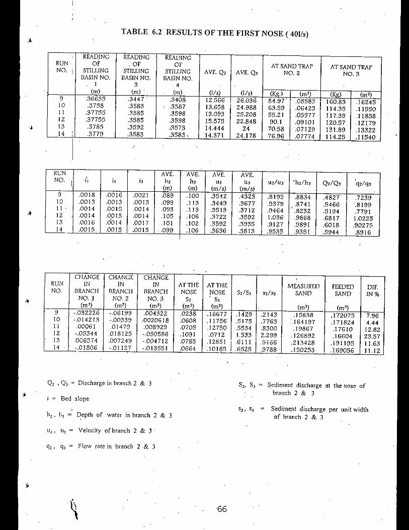
TABLE 6.2 RESULTS OF THE FIRST NOSE (401/s)

Sediment discharge per unit widthof branch 2 & 3

52. S3 = Sediment discharge at the nose ofbranch 2 & 3

66

"

READING READING READINGRUN OF , OF OF AT SAND TRAP AT SANDTRAFNO, :: STILLING STILLING STILLING AVE, Q2 AVE. Q, NO.2 NO.3BASIN NO, BASIN NO, BASIN NO.

I 3 4(m) (m) (m) (IIs) (lIs) (K~.) (m') (K,s() (m')

9 ,36635 .3447 ' ,3408 12.566 26,036 84.97 ' .08583 160,83 ,1624510 .3758 .3583 .3587 13.658 I 24.988 63.59 .06423 114.35 .11550I I .37755 .3585 .3598 13.093 .25.208 55.21 ,05577 \17.39 .1\85812 ,37755 .3585 .3598 15.575 22.848 90.\ .09101 120.57 ,12\7913 .3785 .3592 ,3573 14.444 24 70.58 ,07129 131.89 .\332214

"

.3779 ,3583 .3583, 14.371 24.178 76.96 .07774 114.25 .11540

Q, ,Qj. ~ Discharge in branch 2' & 3

i ~ Bed slope

U" u, ~ Velocity of branch 2 & 3 .

q,. q, ~ Flow rate in branch 2 & 3

h,. h, ~ Depth of water in branch 2 & 3

RUN AVE, AV.E. AVE. AVE. ,NO.t

-j'] i2 ;, h2 h, U2 U, Uz/U3 thz/h3 Q2/Q, q2/q,(m) (m) (mls) (ml s)

9' ,0018 .0016 .0021 .089 .100 ,3542 .4323 .8195 .8834 .4827 .723910 .0013 .0013 .0013 .099 .113 .3449 .3677 .9379 , .8741 .5466 .8199I 1 ' .0014 .0015 .0014 .093 .113 .3513 .3712 .9464 .8232 .5194 .7791 ..12

'I

.0014 .0015 .0014 .105 .106 .3722 .3592 1.036 .9868 .6817 1.022513 .0016 .0'014 ,0017 ,101 .102 .3592 .3935 .9127 .9891 .6018 .9027514 .0015 .0015 .0015 .. 099 .106 .3636 .3813 .9535 .9351 .5944 .8916

CHANGE CHANGE CHANGE. . .

RUN IN IN IN AT THE AT THE MEASURED FEEDED DIF.NO, BRANGI BRANCH BRANCH NOSE NOSE S2/S, 5Z/ S3 SAND SAND IN%NO. ,1 NO.2 NO.3 S2 • S,(m') (m ') (m') (m') (m') (m') (m')

9 -.032226 -,06199 .004322 .0238 .16677 .1429 .2143 .15838 .172075 7.9610 -,014213 -.00339 .0020618 .0608 .11756 .5175 .7763 .164197 .171824 4.4411 .00061 .01479 .008929 .0705 .12750 .5534 .8300 .19867 .17610 12.8212 -.05344 .018125 -.050586 .1091 .0712 1.533 2.299 .126892 .16604 23.5713 .006374 .007249 -.004712 .0785 .12851 I .6111 .. 9166 .213428 I .191\95 11.6314 -.01806 -.01127 -.013551 .0664 .10185 .6525 .9788 ' .150253 .169056 11.12

••

TABLE 6.3 RESULTS OF THE FIRST NOSE ( 201/s)

Sediment discharge per unit widthor branch 2 & 3

S, ,S, ~ Sediment discharge at the nose ofbranch 2 & 3

67

I

Q, ,QJ ~ Discharge in branch 2 & 3'

i ~ Bed slope

"" ", ~ Velocity orbranch 2 & 3

h" h, ~ Depth of water in branch 2 .& 3

q" q, = Flow rate in branch 2 & 3

Iii

READING READING READINGRUN OF. OF OFNO. STiLLING STILLING STILLING AVE.Q, AVE.Q, AT SANDTRAPNO. AT SANDTRAPBASIN. BASIN BASIN 2 NO.3I NO. I NO.3 NO.4

I (m) (m) (m) (IIs) (1/ s) (K.\1..) (m') (K.\1..) (m')15 .33615 .30723 .30282 5.087 13.639 , 36.32 .05668 'i46.G8 .1481616 .32980 .30723 .29267 8.8563 9.7093 159.78 .16 I39 24.91 .0251617 .33000 .28178 .28147 10.9 7.382 168.78 .17048 6.19 ..00625. 18 .33185 .28220 .28173 7.4081 10.961 36.24 .03660 153',34 .15489,19 .32685 .29486 .29486 6.614 11.77 57.71 .058i9 111.16 .1122820 .32535 .2n26 . .29348' 6.116 12.i93 4.3.5 .04394 126.6 .1i78821 .32471 .29426 .29788. 4.9433 13.727 5.82 .00588 135.58 .13695

RUN AVE. AVE. AVE. AVE.NO. iI ;, h h, h, u, u, UZ/U3 h,lh, Qz/Q, q,/q,

" (m) (m) (m/s) (mls)15 .0024 .0021 .0027 .0440 .0598 .289 .380 .7604 .7358 .3730 .559516 .. 0023 .0014 .0032 .0726 .0450 .305 .359 .8~82 1.613 .9121 1.36817 .0037 .0037 .0038 .0608 .0354 .448 .347 1.289 1.718 1.477 2.21518 .0038 .0038 .0039 .0466 .0456 .397 .401 .9918 ' 1.022 .6758 . 1.01419 .0025 .. 0024 .0025 .0499 .0556 .331 .353 .9372 .8993 .5619 .842920 .0025. .0025 .0025 .04671 ' .0572 .327 .355 .9198 .8180 .5016 .752421 .0022 .0024 .0020 .0414, .0661 .298 .346 .8619 .6267 .3601 .5402

CHANGE CHANGE CHANGERUN IN IN IN ATTHE ATTHE MEASURED FEEDED DIF.NO.. BRANCH BRANCH BRANCH NOSE NOSE Sz/S, 82/53 SAND SAND IN%

NO.1 NO.2 NO.3 S, S,.(m') (m') (m') (rh') (m') • (m') (m')

15 -.02 -.01911 -.01423 .01'758 .13393 .13124 .19686 .131507 .145912 9.8716 -.02045 -.06653 .030393 .09486 .0555 1.7076 2.5614 .129967 .152122 14.5617 -.01146 -.03615 .019094 .13434 .025346 5.2999 7.9498 .148245 :163522 9.3518 -.00483 .057799 -.09106 .09441 .0638211.4791 2.2186 .153396 I ~163522 6.'1919 .-.01669 .006684 -.00847 .06498 .103815 I .62:189 .9388 .15210 .15195 , .10020 .012385 -.00747 .002907 .03646 .130785 .2788 .4182 .1796351 I .15195 18.2221 .006485 .02745 -.00352 .03333 .133429.2498 .3747 .173245 .156604 10.63

TABLE 6.4 RESULTS OF THE SECOND NOSE (30 I/s)

RUN AVE. AVE. AVE. AVE.NO. I' i,- i, ;, h2 h, U2 U, Uz/U3 h2/h, Q2IQ, ' q2/q,

(m) (m) (mls) (mls)22 .00165 ,00157 .00174 .0570 .0961 .2842 .3874 .7337 .5933 .29024 1.161 '23 .00188 .00184 .00193 .0424 .0969 .2648 04107 .6448 04374 .1880 .752024 .00175 .00199 .00149 .0375 .1078 .2596 .3808 .68 I 7 .3478 .1581 .632325 .00188 .00197 .00178 .0342 .1029 .2464 04063 .6065 .3319 .1342 .5367 '26 ' .00194 .00196 .00192 .0342 .1004 .2456 A I 62 .5901 ' .3406 .1339 .535927 .0015 .00136 .00164

.0811 .0839 .3151, .3523 .8944 .9672 .5767 2.30728 .00165 .00149 .00181 .05,7 .0924 .2838 .3883 .73 I I .6464 .3150 1.26029 .00192 .00186 .00198 .04 t 9 .0961 .2646 A I38 .6394 04359 .1858 .743330 .00195 .00191 .00199 .0387 .0973 .2582 04171 .6191 .3979, I, .1642 ' .6570

Sediment discharge per unit widthof branch 2 & 3

S2' S3 = Sediment discharge at the nose ofbranch 2 & ,3

68

READING READING READINGRUN or or orNO. . STILLING STILLING . STILLING AVE.Q2 AVE.Q3 ATSANDTRAP ATSANDTRAPBASIN BASIN BASIN NO.2 NO.3NO.1 NO.3 NO. 4

(m) (m) (m) (1/ s) , (I/s) {~.) {ni3) {~) {m3}22 .37615 .35517 .354134 I' 60484 22.34 7.38 .00745 W5.8 .1674723 .3782 .35392 .353484 40494 23.904 3 .00303 137.74 .1391324 .37975 .35472 .359334 3.8972 24.654 4.14 .00418 154.02 .1555725 .37856 .35312 .355134 3.3678 25.097 1.75 .00177 149049 .151026 .37926 .35368 .354434 3.361 25.083 4.68 .00473 147. I6 .1486527 .38055 .36210 .359984 10.228 17.734 3.25 .00328 70.25 .0709628 .38290 .36257 .360234, 6.785 21.5378 1.69 .00171 138.5 .1398929 .38560 .36100 .360334 '40434 23.8(>2 .14 .00014 114.19 .1153430 .38650 .36127 .361034 4.00 24.353 3.78 .003,82 123.9 .12515

-hi, h) = Dcrth of \Voter in brAnch 2 & 3

Q2 ,QJ = Discharge in branch 2 & 3

i = Bed slope

Q2' qJ = Flow rate in branch 2 & 3

Uz, tI) = Velocity of branch 2 & 3

CHANGE CHANGE CHANGE ATHIE ATTHERUN IN IN IN NOSES2 NOSES, MeASURED rEEDED DIP.NO. BRANCH BRANCH BRANCH S2IS3 82/83 . SAND SAND IN%NO. I NO.2 NO.3

(m') (m') (m') (m') (m') (m3) (m3)22 -.01735 .072973 -.02 I95 .08043 .14552•.5527 2.21 I , ,.20860 .! 7962 16. I323 .01001 I ,020720 .020199 .02375 .I 5933 ,1491 .5964 .19309 .16407 17.6821 -.00517 ,005665 -.02086 .00985 .13471 .073 I .2924 .13909 . !6825 17.3325 -.01231 .007745 -.00813 .00951 .14287 .0666 .2664 .14007, . I 6729 16.2726 .000934 .001275 -.00395 .00600 .14469 .04 I 5 .166 . I5163 .15476 2.02727 .076726 .058564 -.03408 .06184 .03688 1.677 6.708 .17545 .16100 8.97328 .019848 .072918 -.02387 .07463 .1 1603 .6431 2.572 .21050 .18113 16.2129 .001499 .028753 -.00914 .02889 .1062 I .272 1.088 , .13660 . I 5723 13.1230 .006136 .003844 .006886 .00766 .13204 .058 .232 .14584 .16151 9.705

••

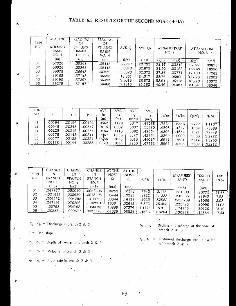
TABLE 6.5 RESULTS OF THE SECOND NOSE ( 40 I/s)

RUN AVE. AVE. AVE. AVE.NO. I, i, h' h, h3 U, U3 uz/u:\ h2/h3 Q,/Q3 qzlq,

(m) (m) (mls) (mls) .

31 .00194 .00196 .00192 0562 .1126 .33 I 7 .44088 .7524 .5536 .2777 1.110732 .00348 .00348 .00347 .0415 .0982 .3607 .55430 .6508 .4227 .1834 .7336933 .00225 .00215 .00234 .0484 .1118 .3062 .48554 .6306 .4332 .1821 .72848" .0958. .3527 .42654 1.009 '34 .00176 .00143 .00211 0~67 .8269 .5568 2.227235 .00177 .00128 .00227 .0,88 .1038 .3013 .46025 .6547 .7591 .3314 1.325536 .00188 .00144 .00233 .0629 .1086 .2850 .47772 .5967 .5798 .2307 .92272

Sediment discharge per unit widthof branch 2 <;0 3

82 • SJ = Sediment discharge at the nose ofbr~nch 2 & 3

69

READING READING READINGRUN or or orNO. STILLING STILLING STILLING AVE.Q, AVE. Q3 AT SAND TRAr AT SANDTRArBASIN BASIN BASIN NO.2 NO.3NO.1 NO.3 NO. 4

(m) (m) (m) (II s) (II s) (Kg.) (m') (K.I() l(m3)31 .37926 .35368 .35443 8.2747 29.799 32.17 .03249 97.54 .09853 •32 .39926 ., .35368 .35443 5.9940 32.679 31.50 .03182 183.65 .1855033 .39508 .36648 .36529 5.9320 32.572 37.36 .03774 170.90 .1726334 .39165 .37142 .3659'8 13.651 24.517 88.76 .08966 127.73 .1290235 .39193 .37297 .36493 ,9.5013 28.673 53.64 .05418 108.70 .1097936 .39275 . .37197 .36468 7.1815 31.132 40.46 .04087 84.64 .08546

Q, , Q, ~ Discharge in branch 2 & 3

h" h) ~ Depth of water in branch 2 & 3

i ~ Bed slope

U" 11) ~ Velocity ofbronch 2 & 3

Q2, q) = Flow rate in branch 2 & 3

CHANGE CHANGE CHANGE AT THE ATTIIE. RUN IN IN .IN NOSE NOSE MEASURED rEEDED Dlr.0

NO. BRANCH BRANCH BRANCH S, S, SzlS3 szlS3 SAND SAND IN%NO. I NO.2 NO.3(~13) (m3) (m3) (m3) (m3) (m3) (m3)

31 .047977 .050040 .0053608 .08253 .10,'3g8 ,7945 , 3. i78

I.234399 , "),,",ooc , !L53

I..L..Vvvv

32 -.001699 ,022620 .0073905 .05444 .19289 I .2822 1.1288 .245635 I .22843 7.5333 .006962 -.004295 -.010655 .03344 . i6i97 .2065 .82588 .2023758 .21066 3.9334 .047491 .076256 -.102901 . I 6591 .02612 6.352 25.408 .239523 .20996 14.0835 -.00798 .054798 ,.036038 .10898 .07376 1.4775 5.91 .174759 .20126 13.1636 .00235 -.000577 .0027776 .04029 .08824 .4566 1.8264 .130888 . I 5834 17.34

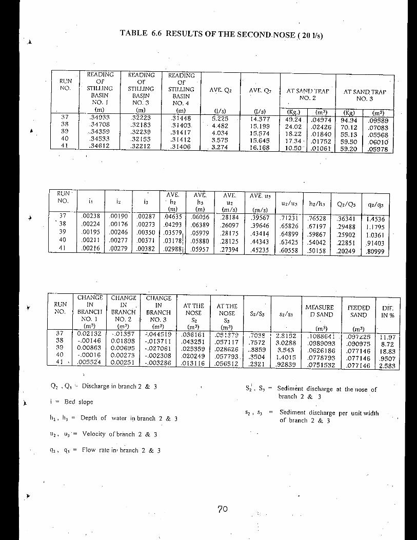
TABLE 6.6 RESULTS OF THE SECOND. NOSE (20 lIs)

RUN' AVE. AVE. AVE. AVE.U,NO. i, iz ;, . h2 h, U, uZ/U:l h,lh, Q,/Q, q,/q,

(m) (m) (mls) (ml s)37 00238 00190 .00287 04635 .06056 28184 .39567 .71231 .76528 .36341 1.4536. 38 .00224 .00176 .00273 .04293 .06389 .26097 .39646 .65826 .67197 .29488 1.179539 .00195 .00246 .00350 .03579 .05979 .28175 .43414 64899 .59867 .25902 1.036140 .00211 .00277 .00371 .03178 .05880 .28125 .44343 .63425 .54042 .22851 .9140341 .00216 .00279 .00382 02988 .05957 .27394 .45235 .60558 .50 I58 .20249 .80999

Sediment discharge per unit widthor branch 2 & 3

Sz:, S) = Sediment discharge at the nose ofbranch 2 & 3

70

READING READING READING

I ,-'"'''".'''RUN or or or!NO. STILLING STILLING STILLING AVE.Q, AVE.Q, AT SAND.TRAPBASIN BASIN BASIN NO.2 NO.3NO. I NO.' 3 NO.4

(m) (m) (m) (IIs) (IIs) (10.) (m') (K.) (m')37 .34933 .32223 .31448 5.225 14.377 49.24. .04974 94.~)4 .0958938 .34708 .32183 .31403 4.482 15.199 24.02 .02426 70.12 .0708339 .34359 .32239 .3'1417 4.034 15.574 18.22 .01840 55.13 .0556840 .34533 32155 .3 I 412 3.575 15.645 17.34 . .01752 59.50 .0601641 .34612 .32212 .31406 . 3.274 16.168 10.50 .01061 59.20 .05978

liZ, ll)'= Velocity ofbraneh 2 & 3

0, . OJ ~ Discharge in branch 2 & 3

q" q, ~ Flow rate in' branch 2 & 3

h2, hJ = Depth of water i!l branch 2 & 3

CHANGE CHANGE CHANGERUN IN IN IN ATTIlE ATTHE MEASURE rEEDED DlLNO. BRANCH BRANCH BRANCH NOSE NOSE S,IS, Sz/S3 DSAND SAND IN%NO. I NO.2 NO.3 S, S,

(m') (m') (m') (m') (m') (mi) (m')37 0.02132 -.01357 '.044519 .036161 f"\~lQ7c.a ""'('l"..z~ , 2.8152 I . I08864lI.097225 11.97.vv ••...' "

I.1 v •...••..

38 -.00146 0.01898 -.0/371 I .043251 .057117 .7572 3.0288 .0989093 .090975 8.7239 0.00863 0.00695 -.027061 .025359 .028626 ..8859 3.543 .0626186 .077146 18.8340 -.00016 0.00273 -.002308 .020249 .057793. .3504 1.4015 .0778793 .077146 .950741 .005524 0.00251 -.003286 .013116 ,056512 .232 I .92839 .0751532 .077146 2.583

). i ~ Bed slope

FIGURES

BIFURCATION

CONFLUENCE,

'Fig, 1.1 THE CONFLUENCE AND BIFURCATION OF RIVERSYSTEM

71

--JI\)

" -.•..'

~

".

q 1 T ~ t 1m

•• ....

I

17 18 19 2b 2\2

..

23 24 .25

Outflow--.

Fig. 2.1 MODEL OFTHE BENI-MAZZAR REACH OF THE NILERIVER.

C/)..JWZZ

~(JClWC>Cl'wn::Cl

wwn::J:I-WJ:l-Ll..oI-Z••••....2zC>:J«N~

.~LI..

E

oN,....,

oco

o'"NI

, .

'c"

,..,''" ' -c.: I' ~

. - ".::- ~w ~- ,~~ i:l.,~ I", :>,.., ,~~.

73

,\\\

\\\\,,,,

; .

J IS"

liT, .

1.1,. )

••Iri

I=!,

CI

1

500 1000

00

So

=.~.=~

Main channel

Secondary channel

2 4 6 8 10 20 40 100 200

U* dBoundary Reynolds number, R* = -v-

Fig. 2.4 SHIELDS DIAGRAM FOR INCIPIENT MOTION

74

0406 1.0

"I

I, ''''

Ps' in gm

'b Ambe'}

per cu em1.06

• lignite (Shieldsl 1.27o Granite 2.7o Barite . 4.25, Fully developed turbulent velocity profile S C

2.65II I I I ! I I I. i I I * and ( asey)IIIII I . + Sand (Kramer) 2.65. : I ~ Sand(U.S. WES.) 2.65

Sand (Gilbert) . 2.65{. Sand (While). 2.61

Turbulent boundary I~yer' 0 Sand in air (White) 2.10'1 • i", "(T 1 "" Sleel shot (White) 7.9,

Value 01.2.. j 0.1 ( Y s .1) gdl' v Y"-

2 4 6 8 10 2 4 6 100 2 4 611000•

--A / / / 1// II / J../ -,fftTl..I ,,,''It ..-..: \ 0

I I v ~ Shtldf frve

0.10080.060050040030.02

02

Fig. 2.3 SCHEMATIZED MAIN AND SECONDARY CHANNEL'SYSTEM

(f)(f)Q)~~(f)

(f)(f)Q)

co(f)cQ)

Eo

u,s.:- 10

1:'.0806

II 0.5~ 04

0.3

)

1m <5/3 I

unstable:

. c:=::C> saddle point

==t>sink

75

!

Fig. 3.1 PHASE DIAGRAM IN CASE OF m < (5/3)

Fig. 3.2 PHASE DIAGRAM IN CASE ,OF m > (5/3)

"

'.

..•. ~ .(. .•.. '0- I-

>:•••w'"l-V>0..=>

'"o5:wVl"-''"

o

STILLING BASIN

OOWNSTREAMRESERVOIR

=,..~~1'-'

"

REHBOCK WEIR

<==FLOW OIRECTION

i1.' -

J-'

--..J(J\

-PIPE LINE

.Fig. 4.1 GENERAL LAYOUT OF THE SET-UP

DoPERMANENT' PART

77

TEMPORARY PART

Fig. 4.2 LAYOUT OF THE MODEL SHOWING TWO' PARTS

"'I•• I4.55m

FLOW DIRECTION

WOODEN NOSE,

1489 m

' .•• I ).15m •. I ••6.19m

BRANCH 2

BRANCH 3 .

Fig. 4.3 LAYOUT OF THE TEMPORARY PART

78

, '

, .'

SANDTRAPS

I ~1,2.00m I.

TUBES.

12 JJ I

<--FLOW DIRECTION

2.0m ~OJ

I ~---,0.5

BRANCH 2

8'6m'

37

8 7 5 5 4 3

5

~ 2.25m .1.II STILLING BASIN

~ 25

,SANDFEEDER SUPPORTS

79

!1.0m

I

STILLING BASIN IV

Fig. 4.5 DETAIL OF BRANCH 2 AND BRANCH 3

STILlING'BASIN III

STILLING BASIN

l Fig. 4.4 DETAIL OF THE INFLOW ZONE AND BRANCH 1

III

II

IIIIII

I.OOm

branch 1,

I.OOm

branch 1

ILOOm I

I.1

'.

branc,h 1

~O.BOm

.20m

O.30m

,

IO.70m •~

NOSE-l

NOSE -' 2

NOSE- 3

2

2

Fig. 4.6 DETAIL OF THE NOSES

80

,

),

, ,.\"'~I'.:' I: ~

- I

Om lI

.1I

fml SAND

o CONCRETE

~ BRICK-WORK

==-FLOW DIRECTION

SANDTRAP

2.00m

TAIL GATES

2.00m '1PLAN

SA":lDTRAP 3

r-2"OOm, .

I-

I-SIDE VIEW

T'.OOm

-l

81

Fig. 4.7 DETAIL OF THE SANDTRAPS

I, " , ", ,

::5AND',BED: :

T:, '

O.80m'

LiI,L.B. F. , •

. V I."

I

MIN WATER LEVEL

TO.~5m

1

MAX WATER LEVEL

RUBBER FOIL

STEELPLAfE FORGUIDANCE OF FLOW

• I

C.5Cm

•• •••• () iii• •

O.17m'

SIDE V lEW

C.35m

VENTILATIONTUllE 038m

FRONT VIEW

•

• •. .

OJ5m

82

III 'I II I: TAIL GATEI 'II

I1III

Fig. 4.8 CONFIGURATION OF A TAIL GATE

DETAILTAILGATE

0.55 LBF

1.20 L B F

,FREEBOAR D 0.10HEAD LOSS 0.0

HEAD OVER TAILGATE 0.12

0.95LBF

)

DRAIN

/

O. &0 rTI

PILLAR

DOWNSTREAM RESERVOIR

SPILLWAY

,STILLING BASINS

Fig. 4.10 CROSS-SECTION OF THE SPILLWAY

83

=PUMP

..

Fig. 4.9 DOWNSTREAM RESERVOIR

0.77 LBF

DRAIN

a 0

APPROACH

CHANNELS

'"' ' .•, ,..'"" ".,

o

~D

•

SUPPLY PIPE LINEBJ

~PILLAR

I.. 12.90m :~D:rt-_

t l.h"" ,Bd, ) '.t::1? ~E:C:S:p:p:r;" ,4, , , , , , , ,II~~

Fig. 4.11 . LAYOUT OF THE PIPE LINE

,T'82m

0.2m

0.4m

0.6m

85

PUMP

SECTION A-A

SECTION 8-8

0.40.85

LABORATORY FLOOR

Fig. 4.12 SECTION A-A ANDB-B OF THE PIPE LINE

, PILLAR

}

,'

)c t "

0.4m .~+- 'ra0.46m

7.90m

~r• Io I

b 1.60m

, .. 1

o

o.'o

oQ. ""F:

86

o

o 0o 0,

o 0o 000

SECTION D-D

SECTION C-C

.22.15 Eil.20

. 1.25m

~.50mI~

I.

, '

Fig. 4.13 SECTION C-C AND D-D OF THE PIPE LINE

. I

Ti m

--1'~~J

PVC TUBES

6.87m

DRAIN

Fig. 4.14 DETAlL OF THE UPSTREAM RESERVOIR

PIPE LINE

1_' _S_T_I_L L_I_N_G~R__ESE_R_V_O_IR__ ----'--_

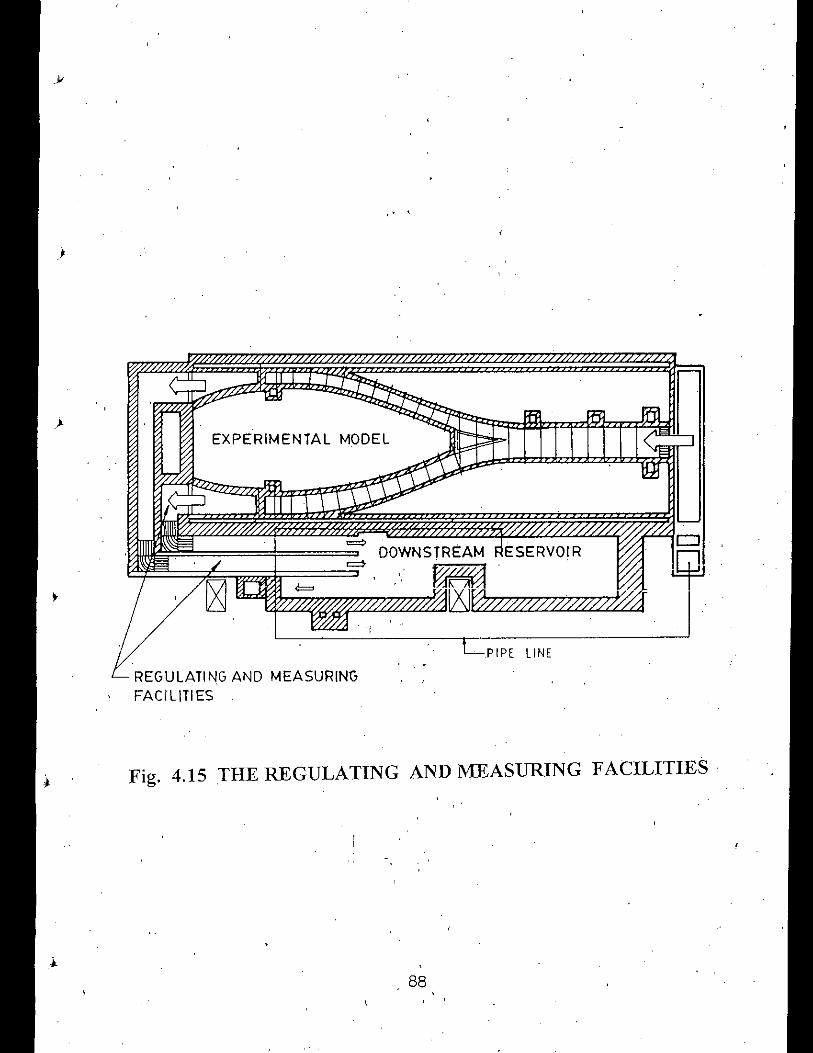
Fig. 4.15 THE REGULATING AND MEASURING FACILITIES.

CJ ,

PIPE LINE

., '

88

, "

" .

DOWNSTREAM.~

l6Ji

REGULATING AND MEASURIN~FACILITIES

REHBOCKWEIRS

R,..,.... . ..~.,

,~"• :. • •• ' •• ': •• ol,."',,'

•• { / : I<== /':; PIPELINESI / 1\, I,

TAil GATE

STilLING BASIN

TUBES

.'

STilliNG BASIN

TAil GATE

PUMP

CHANNELS

APPROACH

STilLING BASINS

. . '.. ,'. ' ,' .. : ..

.. ' .. " ' ....

89

II1;.

TUBES

GUIDINGVANES

TRANSITIONFLUMES

Fig. 4.17, THE APPB,OACHCHANNELS AND THE REHBOCKWEIRS

Fig. 4.16 DETAlL OF THE REGULATING AND MEASURINGSYSTEM

\ '

FOOT RESTBASE PLA TE

f10PPER

VA~I.t..( .DC MOYORGEAR BOX

GEAR PLATEPINIUM

SAND BUCKET

,.I..'

90

o

Fig. 4.18 D1AGRAMATIC VIEW OF SAND FEEDER

0000o

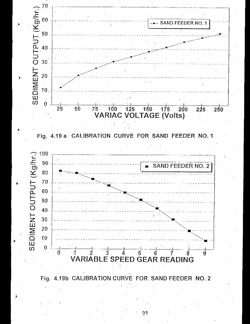
91

__ 70 - ---~---------~------~-------~ _

90 - -- -~-~ . - -- -- -- -- c -- -- -- -- - r;:-SAND-FEEDEI~-r;:io.-:q80 - -------~ .•. ---- ---------.---------- __. . _

--------------.70 ">---

6 O' - - - - - - - - :-- -•• - - - _.- - .~,~-~: : :: - - - - - • : : • : - - - : . : - - _:.: : . - -- - . - .~

50 . - - - - - - - _.. - - - - - - - - - - - - - - - - - - - - - - '-- - ~'----'-- _- - '- - __ _~,

40 . _. - - - - - - - - - - , - - - - - - - - - - - - - - - , - - - - ~_ . _.: _

30 . - - - - - - - - - - - - - - - - - - - - - - - - - - - . __ _ .• ~ . __ _ _ __

~~ _-.:::. _::: ---. : -:::. : --:-:: - -:. _ --il~~ __

Fig. 4.19 a CALIBRATION CURVE FOR SAND FEEDER NO.1

.Fig. 4.19b CALIBRATION CURVE FOR SAND FEEDER NO.2

--::- 100 - ---------.------------~~~---. --.------- .__.. .L...c-OJ~---I-:J~I-:JoI-Zill~

oillen O---t-.1----1--j~t---~.------~--'.c.--t----t--.--~--'

VARIABLE SPEED GEAR READING

L...c

. ~6 0 ---,--_--------------- -------: --------------.r::~:-SA-ND.FEEDERNQ1-1- --- - --- - ----I- 50 --.---------.. -.-. -- ---------------------.--------- -------c' ... - - - ~o"- -----_ •..-_....-.:J ..---~ -~40 - -- .-- - - - - - - -- - - - - - - - - - - - - -._.- - - . .,,-. _"__.. . _I- .-~:J -•.------------

-~a 30 .. _..._.._..- - . - - ..._..-~~;.?-~~~------------_.---_..----._...I- ~~~ 20 --7-------------------------- ------

•o 10,-. ---.---- .-------------------------------- .. _--.--.--.------_. -----illen

92

- ,

DIAMETER (mm)

,,-' I -I

Ii .

I.

. ,-

,ASf-.- m FORE IN

~. \111 cr<

A0rliN'

I ,0.000.01

10.00

Li0 ..00

50.00

60.00

]0.00

30.00

100.00

90.00

GRAIN SIZE DISTRIBUTION

.20.00

110.00

0': 80.00W.zH

LLf-'ZWU0':WCL

. Fig. 4.20 THE GRAIN sIZE: DISTRIBUTION OF WASHED ANDUNWASHED SAND

BED-FORM

93

SAND BED,

PIN!r SQ~ARE PLATE

----- ------- ---~ -----,I1IIII1

IIII

I, I,

Fig. 4.22 DETAIL OF THE SPECIAL PIN

Fig. 4.21 DETAIL OF THE 'STILLING BASINS

BRANCH 3STILL ING BASIN III

I ,

STILLING BASIN IV BRANCH

~FLOW DIRECTION

1-, --IIIIIIII

IIIIIII

IIIIIIIII

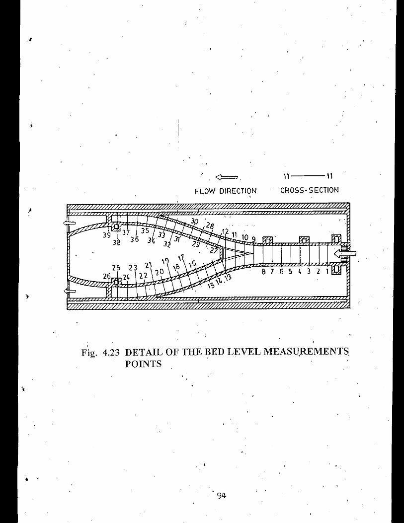
Fig. 4.23 DETAIL OF THE BED LEVEL MEASU.REMENTS,POINTS

11 11

CROSS- SECTION

87654321

., 1110

, ,

94

. "

. <:==.FLOW DIRECTION

•

i!

25 226 24

'>if

1.00

,." ",' , 'liOi--- ...::.- ~J

N

V1 '0.1I0-~V1--~0'

~ 0:60r.

"~•...-cE 0.. 40"'0~ .,\J"IV1.,.:= 0.20-".,0::

0.000.40

••

I I I I

0.52 0.64 0.76 0.88.

Relative Dis~harge (Ql/Q2 )

. Fig. 4.24 RESULTS OF THE TEST RUNS'

.J

--'.'1.00

~Z

, """....:l~;::.~

~~f-<~o'f-;~o>,~~

W0-0-

96

,o,

a.a_<:::>_"'" Q.. ~",

Ew 00- a>0- N

::;0-0-::JIf)

1______.

BRANCH 2

97,

BRANCH 3

BRANCH 1

BED LEVEL EVOLUTION

RUN NO.1

350

'SO

E 300

5- 250..JfOl:> 200

fOl.J 150'Q~ 100CQ

SO

8300

5- 250..JfOl> 200fOl~ 150Q~ 100CQ

Fig. 6.1

~e 300

5- 250..JfOl

200:>fOl..J 'SOQfOl 100CQ

SO

.;

BRANC:: j

98

BRANCH 2

BRANCH 3

BED LEVEL EVOLUTION

RUN NO.2

50

50

_ 350

E 300E:; 250

W 200

1U...J 150

C 100WlD 50

350

E 300E::J" 250

~..J 200150

oW 100lD

350

E 300E-'250..JW 200

1U...J 150oW 100lD

Fig. 6.2

BRANCH 1

BRANCH 2

BRANCH 3

"

E 300

!- 250...<

"";;> 200

""~ ISOCl

""~ 100

350

350

"

S 300

8-- 250...<~ 200

""...:l ISO

Cl~ 10(1o:l

RUN NO.3,

350

"

- 3008.5 250

...<~ 200;>-

""...J ISOCl

""CQ 100

Fig. 6.3 BED LEVEL EVOLUTION

BRANCH 2

BRANCH 3

BED LEVEL EVOLUTION

RUN NO.4I

__ JIlO

Eg 250

..l'-'l> 200

'-'l..J I SO

o'-'lQ:l 100

3"

"

"

E JIlIl

g 250..l~ 200

'-'l....J l!'ill

o~ 100"l

3"

_ 300

E5250..l'-'l> 200

'-'l....J lSI)

fJl:l:l 100

3"

Fig. 6.4

101

RUN NO.5

3"

300...l

"" 25.>"" '00...lCI 15.""~

10.

"

BRANCH 2

3"

300

...l

"" 25.>"" 20'...lCI

"" 15'~

10.

"

BRANCH 3

35.

300

...l""..,

>..,20'...l

CI.., 15.~'00

"

Fig. 6.5 BED LEVEL EVOLUTION

BRANCH 1

BRANCH 3

BRANCH 2

JSO

SO

E 300

5250...:I~ 200;;-

'"~ 150~'"~ 100

SO

102

JSO

RUN NO.6

350

_ 300e!. 250...:I'";;... 200

'".....:l ISO

~'"~ 100

Fig. 6.6 BED LEVEL EVOLUTION

8' 300e- 250...:I'" '00;;-'"...:I ISO~'" 100o:l

SO-f.

Final Bed Level

BRANCH 1

BRANCH 2

BRANCH 3

,so

so

e 300

e- 250

•••<-l;> 200

<-l~ 150~~ 100

""

SECTION

e 300

e- 250

•••<-l;> 200

<-l~ 150

~~ lOll

""

103

so

350

e 300

e- 250

•••s:: 200

<-l...J 150

~~ 100

""

so

,so

RUN NO.7

Fig. 6.7 BED LEVEL EVOLUTION

BRANCH 1

BRANCH 2

BRANCH 3

'"

50

104

__ 300

5g 2S0

..l

'";> 200

'"~ 150Cl

'"c::l 100

350

RUN NO.8

350

- JOO5.e. 250

..l

'";> 200

'"~ ISOCl

'"~ 100

Fig. 6.8 BED LEVEL EVOLUTION

E 300

5-- 2S0..l

'" 200>-'"..l 150Cl

'" 100o:l50

'"

"

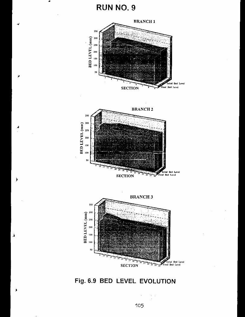
BRANCH!

BRANCH 2

BRANCH 3350

50

RUN NO.9

_ JOO

e5250...J'"> 200

'"....J 150Q

'"= 100

105

8' ;lOO

e- 250...J'"> 200

'"~ ISOQ~ Ion<:Q

350

350

50

_ 300

e-! 250...J'"> 200

'".J ISOQ

'"l%l 100

Fig. 6.9 BED LEVEL EVOLUTION

BRANCH 3

350

so

106

12 27 2829 30 31

32 33 3••SECTION 35 " ,

"

E 300

e-- 250...l~ 200

~- 150o~ 100

350

RUN NO~10

SECTION

"

~E3 300

e'-' 250...l~ 200;>'"..J 150

oW 100<Xl

350

BRANCH I

e 300

e-- 250...l'";> '00

'"~ 150

oW 100<Xl

Fig. 6.10 BED LEVEL EVOLUTION

BRANCH 1

BRANCH 2

__ 300

eg 250

.l<-l;> 2011

<-l.....:l 150

Cl<-lCO; 100

50

BRANCH 3

50

SECTION

107

350

e JOO

e'-' 2.!iO.l<-l;> 200

<-l~ 150Cl~ 100=

350

350

RUN NO. 11

_ 300e,g 150

.l~ 200

j ISOCl<-l.co. 100

Fig. 6.11 BED LEVEL EVOLUTION

••

BRANCH 1

BRANCH 2

BRANCH 3

108

e 300

e-- 250

'"~ 200

~_ 1.50

Q~ 100<Xl

JSO

JSO

RUN NO. 12

so

350

e 3{10e'-' 250

'"<-l;;> 200

<-l~ I~O

Qw 100<Xl

~E 300

e- 250

'"<-l;> 200

<-l.....J 150Q~ 100<Xl

Fig. 6.12 BED LEVEL EVOLUTION)

BRANCH!

BRANCH 2

BRANCH 3

,so

so

so

17 18 19 •20 21

SECTION U 2J 24 25

109

__ 300

e! 250

..lOJ:> 201)OJ~ 150CiOJCQ 100

SECTION

'so

e 300

e'-" 251)..lOJ;;> 200

OJ~ 150Ci~ 100

>50

,so

RUN NO. 13

5' 300

! 250..lOJ;;> 200

eJ ISOCiOJ!Xl 100

Fig. 6.13 BED LEVEL EVOLUTION

BRANCH I

BRANCH 2

BRANCH 3

'"

.- 300E!. 2S0...l~ 200

'"..J 150CI'"Cl:l 100

110

"

'SO

RUN NO. 14

,so

.- JOUES2S0...l'">- 200

'"~ ISOCI

'"Q:l 100

Fig. 6.14 BED LEVEL EVOLUTION

5' 300

E-- 250...l"" 200;;.

'"...l 'SOCI'" 100Ol

"J

BRANCH I

BRANCH 2

BRANCH 3

3SO

50

E 300

Ei- 250...l~ 100

~150

Q

'"~ 100

so

111

50

5' 300Ei-- 150...l~ 200

~ 150

Q.c.:l 100>ll

350

350

RUN NO. 15

E lOll

Ei'-' ISO...l'";> 200

'"...l 150

Q

'"~ 100

Fig. 6.15 BED LEVEL EVOLUTION

BRANCH 2

50

RUN NO. 16

BRANCH 3

BRANCH 1

112

50

_ 350

E '300E:;- 250

W 200>W-J 150

o 100WCD 50

'50

E 300E- 250'...JW 200>W-J 150,

oW 100CD

, 350

,E 300E:; 250

~ 200

..J 150

oW 100CD.

Fig .. 6.16 BED lEVEL J:VOLUTION

113

50

12 13 14 .15 16 17

18 19

SECTION

Fig. 6.17 BED LEVEL EVOLUTION

300E..s 250

--'W 200>W--'o 150WOJ 100

RUN NO. 17BRANCH 1

350

_ 300

ES 250

--'W 200>W--'0

150WOJ 100

50J

36 7

SECTION •

350

300E

~j ..s 250

--'W 200>W--'0 150WOJ 100

50

32 33

1 SECTION 38

BRANCH 3

350

50

350

BRANCH 3

SECTION

SECTION

350

E 300E- 250..J~ 200W...J 150oW 100lD

BRANCH 2

BRANCH 1

114

RUN NO.18

E 300E- 250..J

~ 200W...J 150o~ 100

50

350

E 300

g 250..J

. ~ 200

. ...J 150o~ 100

50

Fig. 6.18 BED LEVEL EVOLUTION

BRANCH 1

BRANCH 2

BRANCH 3

.50

_ 300E..s250...JW 200>W...J 150oWCO 100

350

RUN NO. 19

_ 300

Eg 250

...JW 200>W...Ja 150wOJ 100

•SECTION

50

350

115

50

Fig. 6.19 BFD LFVFL EVOLUTION

_ 30Q

Eg 250

...JW 200>W...Jo 150WOJ 100

,so

so

so

116

,so

RUN NO. 20

..- 300ES 250...:l'-'l;> 200

'-'l...:I 150Q'-'l=: 100

8' 300

E- 250...:l~ 200

'-'l~ ISOQ~ 100~

-. 300E.!250...:l~ 200•••'-'l...:I 150

.f;j.=:l; 100

Fig. 6.20 BED LEVEL EVOLUTION

BRANCH I

BRANCH 2

BRANCH 3

117

BED LEVEL EVOLUTION

_ 300e!, 250...l~ 200

,J 150Q

'"~ 100

50

350

E 30G

!, 250...l~ 200

'"~ 150Q~ 100~

350

350

RUN NO. 21

'5300

5250...l~ 200;;.~ 150Q

'"~ 100

F'g 1::.2".I • v

BRANCH 1

50

'50

E 300E::i' 250

g; 200W..J 150

oW 100[J)

BRANCH 3

50

118

BRANCH 2

_ 350

EE 300

:; 250

~ 200W...J 150

Q 100W[J) 50

_ 350

E 300E- 250..JW 200>W...J 150

o 100WCll

RUN NO. 22

Fig. 6.22 BED LEVEL EVOLUTION

BRANCH 1

119

RUN NO. 23

350

50

_ 300

E..s 250...JWiii 200...Jo 150

WlD 100

6SECTION

BRANCH 2350

300E.s 250...J

~ 200W...J

0 150Wm 100

50

2629 30 31

32 33

SECTION 38

BRANCH 3350

300E.s 250...JW> 200W...J

0 150Wm 100

50

16 17 18____ . ~~ 20 21.:-~'_- ! !(l!'l

Fig. 6.23 BED LEVEL EVOLUTION

BRANCH 2

BRANCH 3

SECTION

50

350

E 300E- 250...J

~ 200

...J 150oW 100m

50

SECTION

RUN NO. 24

BRANCH 1

50

350'

E 300E:; 250

g! 200W-J 150oW 100m

120

350

E 300E- 250...JW 200>W...J 150oW 100m

Fig. 6.24 BED LEVEL EVOLUTION

BRANCH 3

121

50

50

BRANCH 2

350

E JOOE- 250...J~ 200W-I 150oW 100III

RUN NO. 25

350

E JOOE- 250...JW 200Gj...J 150oW 100III

Fig. 6.25 BED LEVEL EVOLUTION

'" BRANCH 1

350

E 300E::i' 250W 200>W...J 1500 100WIII 50

i6 7

SECTION

50

BRANCH 2

BRANCH 3

• "11 122728' 2930313233343536 .

SECTION 37 38

50

50

BRANCH 1

122

RUN NO. 26

350E 300E:; 250

~ 200

W...J 150

CW 100lD

350

E 300E- 250...J

~ 200W...J 150CW 100OJ

350

E 300E- 250...J

~ 200

...J 150

CW 100OJ

Fig. 6.26 BED LEVEL EVOLUTION

I

50

RUN NO. 27

350

910111213141516

17181920 -

SECTION 21 22 232425

BRANCH 3

50

50

BRANCH 1

350

123

SECTION

E 300

E- 250-oJW 200[ij..J 150oW 100m

350

910111227 28 29

30 31 3233 34 35

SECTION 36 37 38

E 300

g 250-oJW 200[ij-oJ 150oW[Q 100

E 300

~ ,250

-oJW 200[ij-J 150oWCO 100

Fig. 6.27. BED LEVEL EVOLUTION

124

RUN NO. 28BRANCH 1

350

_ 300

Eg 250

-'W 200>W-'0 150Wm 100

50

6

SECTION

BRANCH 2

350

300

Sf g 250

-'W 200>W-'0 150Wm 100

50

33

SECTION

BRANCH 3

350

300

Sg 250

-'W 200>W-') 0 150Wm

100

50

19SECTION

Fig. 6.28 BED LEVEL EVOLUTION

Final Bed Level

BRANCH 3

9 10111".<.1314,'5

16171819 202122SECTION 23 24 25

6 10 11 12272829303132333435SECTION 36 37 36

50

125

50

E 300

E- 250..JW 200

iii...J 150oW 100al

350

50

BRANCH 2

6

SECTION

350

E 300E- 250..JW 200>W...J 150oW 100al

RUN NO. 29

BRANCH 1

350

E 300

E- 250..JW 200>W...J 150

oW 100al

Fig. 6.29 BED LEVEL EVOLUTION

;

t

9

, 1

, I

I

BRANCH 1

!

.11.

BRANCH 2

BRANCH 3

5

,.

47

SECTION

3

i ..9 10 .;, i11122728 ' . , .

29 30 31 32 nWal Bed Level333435 ISECTION 363738 Flna Bed Level

50

50

350

E 300E- 250-'W 200>W...J 150aW 100W

350

E 300E- 250-'W 200>W..J 150aW 100W

50

126

RUN NO. 30

350

E 300E:; 250

~ 200W-I 150aw 100W

Fig. 6.30 BED LEVEL EVOLUTION

1

1

s.

BRANCH 2

BRANCH 3

s.

35.

E 300E- 250..JW 200

Gi...J 150CW 100lD

BRANCH 1

127

s.

RUN NO. 31

350E 300E:; 250

~ 200

..J 150

~ 100lD

35.

E 300E- 250..JW 200

Gi..J 150CW'00lD

Fig. 6.31 BED LEVEL EVOLUTiON

50

BRANCH 2

BRANCH 3

50

350

E 300E- 250..J

~ 200

...J 150aw 100en

BRANCH 1

128

50

RUN NO. 32

350 i

E 300E:; 250

~ 200W...J 150

aw 100en

350

E 300E- 250..JW 200>W...J 150aw 100en

Fig. 6.32 BED LEVEL EVOLUTION

'0

129

'0

RUN NO. 33

'0

tlRANCH 1

350

E 300E- 250-JW 200>W-' 150CW 100CO

BRANCH 3

BRANCH 2

350E 300E3' 250~ 200W...J 150

fa 100CO

350

E 300'

E- 250-JW. 200(tj-' 150CW 100CO

Fig. 6.33 BED LEVEL EVOLUTION..•

BRANCH 1

BRANCH 3

BRANCH 2

50

9 10 11 1213 14 15

161718 19 20 21SECTION 22 23 24 25

50

130

350

350

RUN NO. 34

SECTION

50

E 300

.s 250

--'W 200>W...J 150Q

W 100[l]

350

- 300E.s.. 250--'W 200fij...J 150QW1JJ 100

E 300

..5.. ~50

--'W 200fij...J 150QWen 100

Fig. 6.34 BED LEVEL EVOLUTION

3••

BRANCH 2

BRANCH 3

,.

...JW 250>~ 200

Cl 150WlD 100

300

,.

,.

, 7

SECTION

360

131

..J 300

~ 250

~ 200

Cl 1"50WCO 100

BRANCH 1

RUN NO. 35

...JUJ 250>~ 200

o 150WCO 100

Fig. 6.35 BED LEVEL EVOLUTION

Final Bad Level

1011 1227282930

3132333435SECTION ." 37 36

810111213141516 1718'9 .202122

SECTION 232425

350

50

50

50

350

"E' 300E

::; 250

W 200>W-i 150CW 100Cl

BRANCH 1

E 300E- 250...JW> 200W...J 150CW 100Cl

BRANCH 2

7SECTION

132

RUN NO. 36

350

E 300

E- 250-JW 200[jj...J 150CW 100Cl

Fig. 6.36 BED LEVEL. EVOLUTION

,

50

50

BRANCH 3

910111227282930 31 3233

343536SECTION . 37 38

50

7SECTION

,"0E 300E:; 250

~ 200W-J 150oW 100OJ

BRANCH 1

BRANCH 2

350

.E 300E- 250..JW 200>W...J 150

oW 100OJ

133

RUN NO. 37

350

E 300E- 250..JW 200[jj...J 150oW 100OJ

Fig. 6.37 BED LEVEL EVOLUTION

50

350

BRANCH 2

BRANCH 3

9101112272829 30313233

343536SECTION 3738

50

350

E 300

E- 250..J~ 200W..J 150CW 100Cll

50

6SECTION

350

134

RUN NO. 38

BRANCH 1

E 300

.s 250

..J

~ 200

...J 150CWIII 100

E 300

g 250..J~ 200W...J 150CWCD 100

Fig. 6.38 BED LEVEL EVOLUTION

I

50

910111213 '14 15 16

1718192021SECTION 22 23 24 25

135

50

BRANCH 3

910111227 28 29

30 31 3233 34 35

SECTION 36 37 38

50

350

350

350

BRANCH 1

BRANCH 2

SECTION

RUN NO. 39

E 300

E- 250..JW 200>.W...J 150oW 100m

E 300

.s 250

..JW 200ru...J 150oWCC 100

E 300

g 250..JW 200ru..J 150oWCO 100

Fig. 6.39 BED LEVEL EVOLUTION

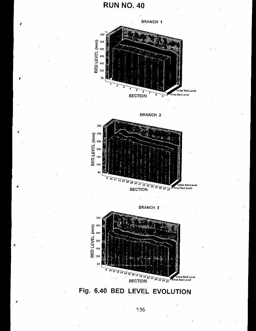
5'

50

E 300

..s 250

..JW 200>W...J 150oWlD 100

350

136

10 11 12 '.131415 16 17 18

," 192021SECTION 22232425

12 27 2829 30 31

32 33 34SECTION 35 36 37 38

50

350

BRANCH 3

BRANCH 2

SECTION

E 300

S 250..JW 200

iii..J 150oW 100aJ

BRANCH 1

- 300E..s 250..Jw 200>W...J 150oWa:I 100

RUN NO. 40

Fig. 6.40 BED LEVEL EVOLUTION

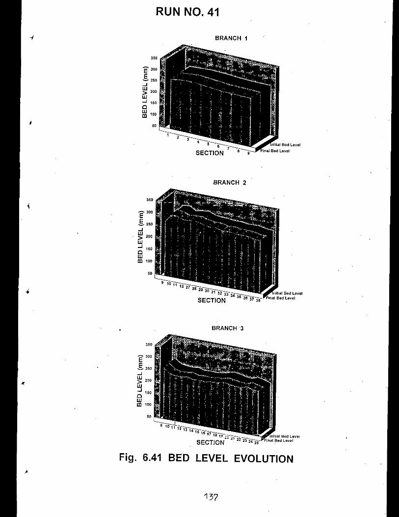
E 300

E- 250..JW 200>W..J 1500W 100CD

I"

RUN NO. 41

'"

9 10 11 1213 14 15

16 17 18 ••, _~_

SECTlo'N"'" 11 22 23" 2425

BRANCH '3

"

BRANCH 1

"

137

'"

'"

BRANCH 2

SECTION 9

12 27 2829 30 31

32 33 34SECTION 35 38 37 38

E 300

.s 250

..JW 200Gj...J 150oWCC 100

E 300

g 250..JW 200Gj...J 150oWIII 100

Fig. 6.41 BED LEVEL EVOLUTION

-.

,.,

,..

5•

•

•

._ _-_ ..-

•

• • •RUN TIME (hi

__ TOTAL I

RUN NO.6

•

, • 5RUN TIME (h)

RUN NO.4

.-.

eO- •.•• •.•

RUN NO.8

. 6 . S 4. .RUN TIME (h)

1 ...• _02

1~~Ql

,.

. 51.3.5 .54.3.5RUNTIME (h)

.' .

......------...-.,._.•.•.'-,•.••~----_.------

-'~--_ ••"•••_.- __ ~~ ••_•••H._.• - __

•

"RUN NO.2

"

"

••lJOW

Ii!~ 20UU>is 10

""

138

FIRST NOSE (30 lis)

VARIATION OF DISCHARGE WITH TIMEFig. 6.42

. -

. 5 7.3

....

. 5 7.3

. 5 7.3

• •• 0

......-.

RUN NO. 10

...---•........,...

. 5 4.3 . 5RUN TIME (h)

RUN NO.12

••• I I "_ ••

. 6 . 5 ~3 . 5RUN TIME (h)

,.

.••~-"'-'--"~~~ ••__~'H~ .••' •••• " __

....... -.-.

10.5 1.3 .5

"

,.

5.

RUN NO. 14

. 6 1.3 . 5 .45 4.3 . 5RUN TIME (h)

,.

_ 40 • --------______...

~w

'"~ 30

U!!1c 2•

7.3

.. .

. 5 7.

. 5 7.3 . 5

• •

.....-----

' ..

__ Q3 .:..•....TOT~q

139

. 5 4. . 5RUN TIME (h)

RUN NO. 11

. 5. 5 1.

Fig. 6;43 VARIATION OF DISCHARGE WITH TIME

RUN NO.13

. 5 1.3 . 5 . 5 4.3 . 5RUN TIME (h)

.51.3.5 .54.3.5RUNTIME (h)

-~ ..

. .. ~._.~.H._. _

.-..--...

FIRST NOSE (40 lis)

"

RUN NO. 9

"

10

10.

"

10

_ 40 . _-- -- .' •.••••••••..•..•..•.•.•. ~

~

"_40

•• !w

'""'30••J:U<IIis 20

• 5

.. .•.

.5

_0'..• .

RUN NO. 16

RUN NO. 20

2.3.5 4. 5.RUN TIME (h)

2.3.5 4. 5.3.5RUNTIME (h)

1.

1.

.-__ • eo '_o'.

HO

__ •••

B

::-:::.:::::---_._. ---_._-........ .• ' ....•.•..•..•.•..• ..-.•.-

_____ ~_~ __ O".O~.__ ~_~ __ .HO•._O_

~---..•.•........

o0.50.51.51. 2.52 3.53.454.54. 5.5556.56. 7.5

RUN TIME (h)

RUN NO. 18

o o.

"

"

oO. 5

""

""

. ....2.. 5 4. 5.3 .5

RUNTIME (hI1.

•. . ....

. ..•.

--,.e._.__ ~ ._. _0' _

o .. ,

"

1D

*- •.

... ......--.-- .....-

140

RUN NO. 21

"

.. .•

2.3.5 •• 5.3 .5RUN TIME (h)

,.

Fig. 6.44 VARIATION OF DISCHARGE WITH TIME

_.oe'~o"o ~ __ eo~o.'~o.oeo ~ ~1

a.a •••.•..••

-_....... . •.•......•....•...

FIRST NOSE (20 lis)RUN NO.15

" r------;::.,~.:~Q;.';.=.~':f_:..:.~~~3=:.:_:,;.;"~O;TP.;l;:;-I----1

RUN NO.19

o~5~51.51. ~5~ 3.5~ ~5~ L5L ~5L ~5RUN TIME (h)

"

o o.

""

,. 5

.-

. 5

•. ..---

. 5

...

.--5.'

4iITOTA~:1

RUN NO. 27

. Ii 4.RUN TIME (h)

.5 4.55.3.5RUN TIME (h)

.5 4.56.3.5RUN TIME (h)

RUN NO. 25

2.'

I~:Q2 ;'" ~__Q3

,. 5

••• ,-O_.~ ~.'•.•.•

1. Ii 2.

1. 5 2.

._--~-_.--..

DISCHARGE WITH TIME

- .•.--~~_. ••_••OHo~O_OHO_._••_••O~.~.-----.~._--~--_.__._-~-~

--_ ..•.-----_.~~-.~..-- .............•..

..• ..

••. 5

••. 5

••

141

RUN NO. 23••

••

_40~w"li1~ 20o'"B 10

A5

. 5

.._ .•...

VARIATION OF

.5 4.55 .. 5RUN TIME (h)

RUN NO. 26

-.- ..

~"OH._~_H,_'H'_~ __ -_

RUN NO. 24

[--:92" '1~~'P3' ~TOTALI

1.52.3,5 4.55.3.5RUN TIME (h)

1. 5 2.3 . 5 4. 5 6.3 . IiRUNTIME (~)

Fig. 6.45a

_~'~'_O__ ~_""'HO_O__ ~.OHoo .•. _

___ • '"O-._.H._._. '"._•••_._OHO•.__.___- ... e.

SECOND NOSE ( 30 lIs)

RUN NO. 22

••. 5

.•.-_•.....•....•....-.-~~~---.-.-.-.•O. 5 1. 5 2.3

••

••~40

W"li1~ 20o'"is 10

••

• •

......

..........

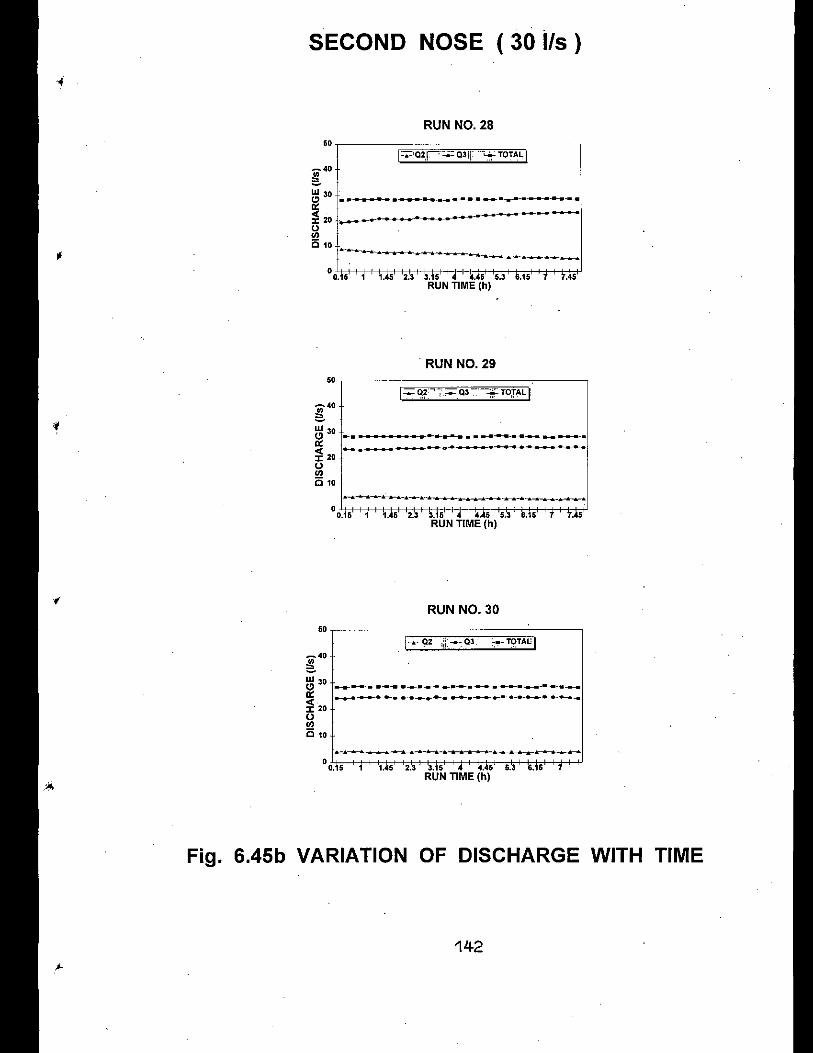
ok •••••••••••

.....

.....

1 • •••• •

•• •••• e

. RUN NO. 29

I.=;:: ~~:""~:';:;::,Q3-:-:'---:g.: ferAL I

I:;::'Q2,1~:;;: Q3iF ...*TOTAL I

1. 2.3 . 5 4. 5 5.3 . 5RUN TIME (h)

1.5 U 15 ~5 a3 L6RUN TIME (h)

....

___ .w' w-.... .

--,-.~.~.--.-.-•.._~-.-.-.-.~..~--.-..~

oO.5 1. 5 2. . 5 4. 5 5.3 . 5

RUN TIME (h)

o o.•

RUN NO. 30

.0

o o.•

.0

142

RUN NO. 28

•• •••• •• ok •• _-' •••••••••••••• _ •..•••••••••...•••

60

-40

~W 30

~~ 20oU>C 10

[40W 30

~~ 20oU>is 10

SECOND NOSE (30 ils )

Fig. 6.45b VARIATION OF DISCHARGE WITH TIME

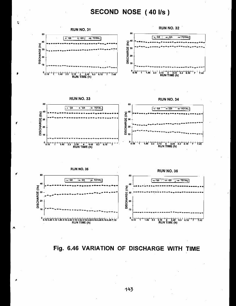
. 5

• •

..

-_\TOTAL::I

RUN NO.3S

-_ .

RUN NO. 34

1"-' 02....

.--•..•-.--.-.-.----------~_......•-

..

1.5 U.5 ~5 U .5RUNTIME (h)

1. 5 2.3 . 5 4. 5 6. 6. 5RUN TIME (h)

1. 5 2.3 . 5 4. 5 5.3 . 5RUN TIME (h)

..

___ .------~-. _ ...•..•• I

..

oO••

RUN NO. 32

••

oO••

60

o o.•

60

40

~w"~ol;:1:"o'"25 10

..

..

...

..

...

~_.•.•...

SECOND NOSE (40 lIs)

>~~~TALI

... -.. ..

..

RUN NO. 31

RUN NO. 33

RUN NO. 35

1.52.3.5 4.55.3RUN TIME (h)

..

1. 5 2.3 . 5 4. 5 5.3 . 5RUN TIME (h)

_.-.~.-.~.-.~.-.----,~.~._~~~.~.---... ..

..... -------------- ..

.. .

__ ._~ •.• ".__ ~-",-----",- ••• I I....................---...-- ..

oO••

o o .•

60

00.150.51.51.52.52.53.53.54.54.55.55. 6.58.5.5RUN TIME (h)

w"~~ 20o!!l010

40

Fig. 6.46 VARIATION OF DISCHARGE WITH TIME

60

143

w"~:<20

11l°10

40

60

~w"~ol;:1:"o'"l5

10

• •

• •2.. 5 4.55.3RUN TIME (h)

RUN NO. 40

•

1.

.. ....--......-.--------.. . . . ..... 1-----1. 5 2. . 5 4. 5 5.

RUN TIME (h)

• •••• -_.~" ~_~. w

RUN NO. 38

......

---"-"-"-' ---~_.~----~-"~.."••••

••

••• •

••_40e.~ 30a::2 20

" I IU)a 10

• G

..

1.52.3.5 4.55.3RUN TIME (h)

......

.1' •• '

SECOND NOSE (20 lIs)

••••

••RUN NO. 41

W 3.

~""J: 2."U)

C 10 .

RUN NO. 37

RUN NO. 39

1. 5 2.3 . 5 4 5 5.3 . 5RUN TIME (h)

.-.~.~._.~.".~.~..~~".~.~._.~.-.~.~._.~--~-.

Fig. 4.47 VARIATION OF DISCHARGE WITH TIME

144

••••

••

a

J;';:':';:;:'~'~';:'::':'~'~';;:'='::;'::,;:~';;'=';;,;'~';:':;':'j'00. 5 ''I '1,'5 2.'3 '3:15 .•• 4.45 5.3 6.15 '1RUN TIME (h)

~40

W 3.

~

~ 20 t::::::::":"::":"::":":"::"::":"::":":":":":":"::":"::":"::"1.•, ••••• 1.Q 10

0.1

I

s2/s3 Vs q2/J3 FOR THE FIRST NOSE (30 I/s)

105 6 7 8 9J2

1q2/q 3

5"6,789J2

145

. ,Fig. 6.48 RELATION BETWEEN SEDIMENT TRANSPORTRATIO AND DISCHARGE RATIO

•

0

0

• 0 ,

i, , I

II

II I

t- o

0

0..

o I)

I

I,

* I,

2

J

5

6

7

7

8

2

J

5

6

9

I

I

10

"II

0. 1

r ..'\,'

M(f)

" 1(\J 9(f) II 8

t

"

s2/sJ Vs. q2/qJ fOR THE FIRST NOSE ( 40 I/s)

0.1 105 6 7 8 975 6 ,7 8 9

. 1q2/q 3

146

2

•

,.

..

. ,

I .I,,

.

,

I

, , ,

J .

I ,

..,

I ,

Fig. 6.49 RELATION BETWEEN SEDIMENT TRANSPORTRATIO AND DISCHARGE RATIO

2

6

5

8

6

9

7

2

5

. '

10

0. 1

M(j)

" 1C\J 9(j) 8

•

s2/s3 Vs 'q2/q] FOR THE FIRST NOSE (20 I/s)

105.6789j25 ,6 7 8 9j ,2

III ' .

" j

//I

, I ' I

/,,

/•j

/I,

/ ••I ' ,

i,

,

, ,

,I .I I I

s

147

9

8

7

8

6

9

7

6

s

0,1

Fig. 6.50 RELATION BETWEEN SEDIMENT TRANSPORTRATIO AND DISCHARGE RATIO

10

0,1

M(j)

'..C\J(j)

(

s2/s3 Vs q2/q3 FOR THE SECOND NOSEC 30, I/s)

J , 52

102 J " 5, 6 7 8 9:3 ~S67a92

I!

--~-~

>

./

I //

, :/>

I*

17 ,

,

11 *

*I

, I , I I ,I I I I I

J

Fig. 6.51 RELATION BETWEEN SEDIMENT TRANSPORTRATIO AND DISCHARGE RATIO

5

98

148

2

5

0. 1,

J

'2

2

J

,

'6

109

87

6

0, 1

M(j)'..,

C\J(j)

1 '

(

s2/sJ Vs q2/q] FOR THE SECOND NOSE( 40 I/s),

,::: ]: , s:101 .

3 ~56789

5

J

2

5

6

149

i

J

, Fig. 6.52 RELATION BETWEEN SEDIMENT TRANSPORTRATIO AND DISCHARGE RATIO

2

6

98

2

.

!

/, , I ,

I, I. '

,

I

!,/

I

,

** I ,,

1

.5

,,. ,

J

II I

.',

, " " - "0,1

109

82

0. 1

M(fJ

"-C\I(fJ

(

s2/sJ Vsq2/qJ FOR THE SECOND NOSE(20 I/s)

2 J .• 5

1023 i56789

, 12 J "56789

Fig. 6.53 RELATION BETWEEN SEDlMENT TRANSPORTRATIO AND DISCHARGE RATIO .

150

0.1

2

5

98

7

6

2

J

,

.

I . . ,-c-

/, /'

I

~

.

II: I

I I

I.

T I

,

5

2

.5

1098

7

6

0.1

M(j)

"C\I(j)

PLATES

PLATE NO. 4.1

PLATE NO. 4.2

151

PLATE NO. 4.3

152

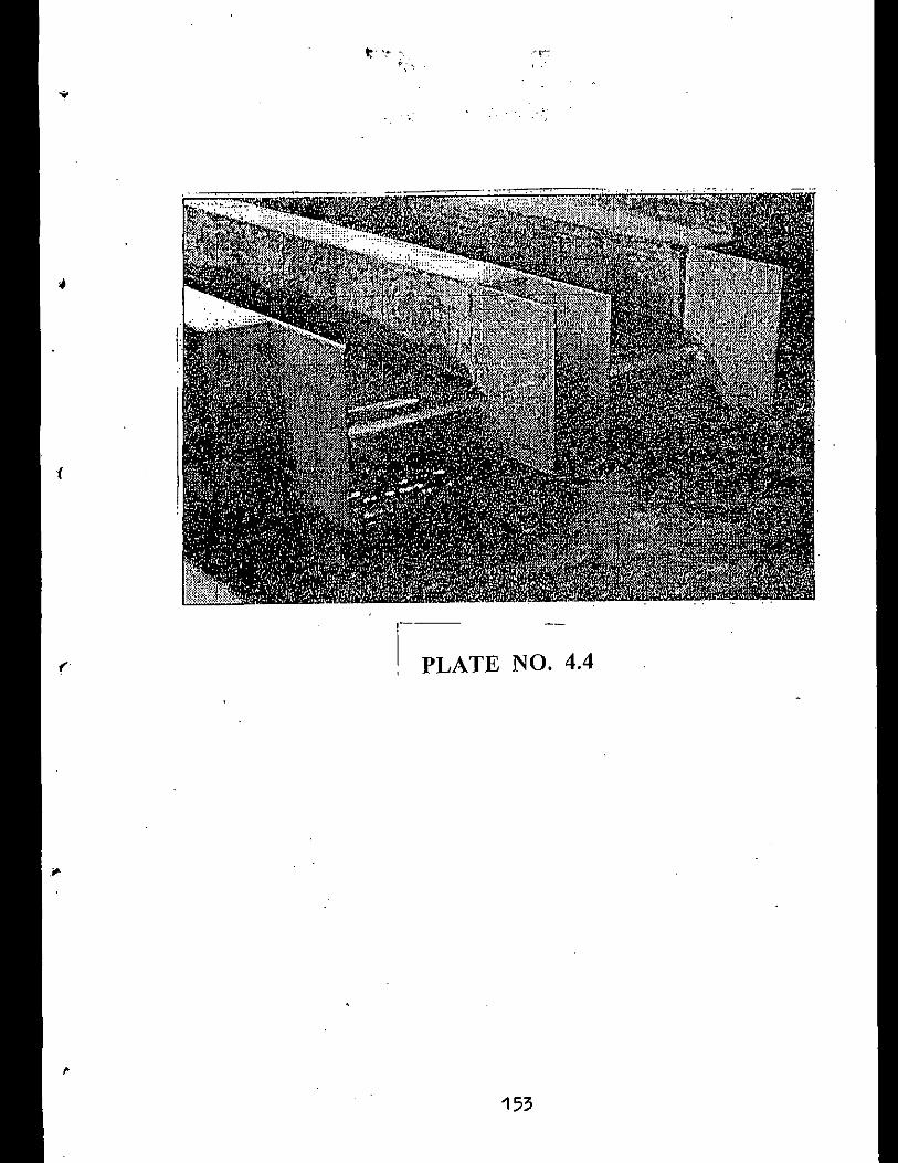
PLATE NO. 4.4

153

PLATE NO. 4.5

154

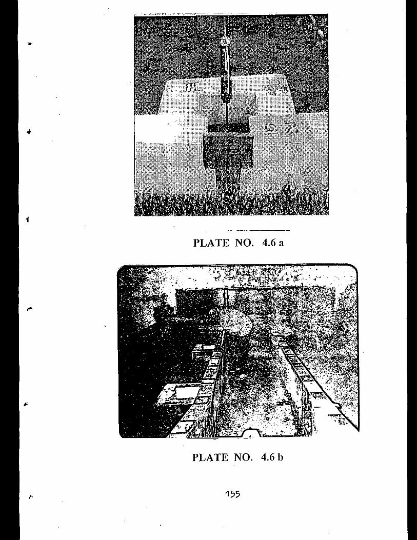
4.6 a

4.6 b

155

]>LATE NO.

PLATE NO.

PLATE NO. 4.7

156

r

PLATE NO. 5.1

157

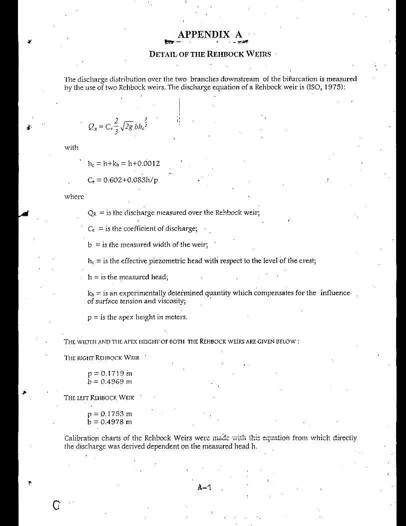
G

APPENDIX A.".... .- . . - ","If

DETAIL OF THE REHBOCK WEIRS

The discharge distribution over the two branches downstream of the bifurcation is measllredby the use of two Rehbock weirs. The discharge equation of a Rehbock weir is (ISO, 1975):

with

he = h+h = h+0.0012

Ce = 0.602+0.083h/p

where

QR = is the discharge measured over the Rehbcck weir;

Ce = is the coefficient of discharge;

b = is the measured width of the weir;

he = is the effective piezometric head witli respect to the level of the crest;

h = is the measured head;

h = is an experimentally detdmined quantity which compensates for the influence.of surface tension and viscosity; ..

p = is the apex height in meters.

THE WIDTH AND TlIE APEX HEIGI.IT OF BOTH TIlE RWBOCK wEiRS AKE GIVEN BELOW:

THE RIGIIT RWBOCK WEIR

p=0.1719mb = 0.4969 111

THE LEFTREIIBOCK WEIR

p = 0.1753mb = 0.4978 m

Calibration charts of the Rehbock Weirs were made '.-,-i:lo :biG eq:.:&tionfrom which directiythe discharge was derived dependent Qnthe measured head h.

A-1

(B. I)

(B.Z)

..

B-1

Co = is the coefficient of discharze;

b = is the measill'ed width of the weir;

The sources of possible error can be identified by examininz Eq.(5 Ii; these sources are:

p = is the apex heizhtin meters. '

h = is the measured head;

he = is the effective piezometric head with respect to the level of the crest;

B.2 SOURCES OF j'OSSIBLE ERROR

kJ,= is an experimentally determined quantity which compensates for the influenceof surface tension and viscosity;

B.l DISCHARGE EQUA nON OF A REHBOCK WEIR IS (ISO, 1975):

ACCURACY OF THE REHBOCK WEIRS

i

APPENDIX B. ,

where

C, ';' 0.60Z+0.083h/p

with he = h+kh = h+0.001Z

1. the discharze coefficient Cc;Z. the dimensional measurement of b;3.. the measured head h;4. the corrective termkh ..

The total error results from'a contribution of'all these errors, According to the quadratic errorpropagation method the relative erro,"on.the rate of flow is calculated with:

"

! QJl = is the discharze nleasured over the Rehbock weir;

The,accuracy of the Rehbock weirs were determined with the help of well-known statisticalI' methods.

r

(B.3)

(BA)

eb = +0.5 mm. ,i, I

From Eq.(B3) it can now be found tnat Xb=+(0.5/500)= +0.1 %.

In Eq. (B2) the relative error in he is-used:

Error in he:

Error in b:

As can be seen in Eq. (B2) the total relative error can be calculated once the individual relativeerrors are found.

The width b was measured with a ruler divided into I nll11intervals; therefore

wh'ere ebcii th'e error in t1;e measurement of width b.

, '

B-2

In Eq. (B2) Xb is defined as:

Error in Ce:, .

In ISO (1975) it can be found that the relative error in the coefficient of discharge can beexpected to be XCe= + 1.0 %,

where

Xh,= is the relative, error in he;

XQR= is the relative error in QR;

B.3 ESTIMATE OF THE TOTAL ERROR

XCe= is the relative error in Ce;

Xb= is the relative error in b;

where

ehl, ehZ,... = are the errors in the measurement ,?f head h;

Given ihis smail value, the contribution of Xb to the total error (see Eq.B2) is considered to be,negligible. "

'. ekh= is the error in the h term;. ,,I,J

\{'-"LJ,1.•.•.~

rI.

20-",=,is the error in the mean of the readings of the head measurement.

According to'ISO (] 975): ekh= 0,3 n1l11.,

The head-!l1easuring device was divided into 0.1 n1l11intervals.

The head h was therefore read to ehl = + 0.05mm; the zero was set to within eh2 = + 0.05' .111111.

The standard deviation in the mean df ten head measurements proved to be d", = 0:03 nllll.I . .r "

It should be realized that Xhe,and tllerefore also XQR, isnot single-valued for a weir: it. willvary with the discharge. A worst-~ase value can however be given: ISO (] 975) sets aminimum value for h: h>0.03 m. As it result:

he 2:0.03+0.0012 = 0.0312 m= Xhe~ + 1.0 %.

Total error:

With the results of the various contributions, the total relative error made for the rate of flow(in the worst-case) can now be calculated using Eg. (HZ).

(B.5)

, ,

B-3

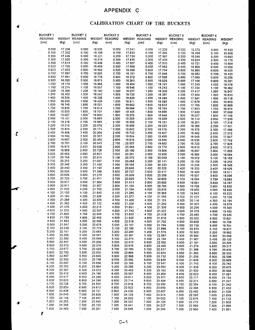
CALIBRAnON CHART OF THE BUCKETS

BUCKET 1 BUCKET BUCKET BUCKET 4 BUCKET 5 BUCKET 6READIN WEIGHT REAOIN WEIGHT READIN WEIGHT READIN WEIGHT READIN WEIGHT READIN WEIGHT(em) (kg) (em) (kg) (em) (kg) (em) (kg) (em) (kg) (em) (kg)

7.500 24.568 7.500 25.369 7.500 24 648 7.500 24.452 7.500 23.053 7.500 22.0847.600 24.673 7600 25.477 7.600 24.752 7,600 24.559 7.600 23.147 7.600 22.1777.700 24.779 7,700 25.585 7.700 24.856 7.700 24.667 7.700 23.241 7.700 22.2707.800 24.884 7.800 25,693 7.800 24,960 7.800 24.774 7.800 23.334 7.800 22,3637,900 24.989 7.900 25,801 7.900 25.064 7.900 24.882 7,900 23.428 7.900 22.4568.000 25.094 8.000 25,909 8.000 25.167 8.000 24.989 8.000 23.521 8.000 22.5498.100 25.199 8.100 26,017 8.100 25.271 8.100 25.097 8.100 23.615 8.100 22.6428,200 25,304 8,200 26,125 8.200 25.375 8.200 25,204 8,200 23.709 8.200 '22.7348.300 25.409 8300 26,233 8,300 25.479 8.300 25.312 8.300 23.802 8.300 22.8278400 25514 8.400 26,342 8,400 25.582 8.400 25.420 8,400 23.896 8.400 22.9208,500 25,619 8.500 26,450 8,500 25.666 8.500 25.527 . 8.500 23,990 8,500 23,0138.600 25,724 8.600 26.558 8,600 25.790 8.600 25.635 8.600 24.083 8600 23.1068.700 25.829 8.700 26.666 8,700 25.894 8.700 25,742,. 8.700 24.177 8.700 23.1998.600 25.935 8,800 26.774 6.600 25.996 8.800 25.850, 8.800 24.270 8.800 23.2926.900 26.040 8.900 26.882 8.900 26.101 8.900 25,957 8.900 24.364 8.900 23.3859.000 26,145 9.000 26.990 9.000 26,205 9.600 26.065 9.000 24.458 9.000 23.4789.100 26.250 9.100 27.098 9.100 26.309 9.100 26.172\ 9,100 24.551. 9.100 23.5719.200 26.355 9.200 27.206 9.200 26.413 9.200 26.280 9.200 24.645 9.200 23.6649.300 26.460 9.300 27.314 9.300 26.517 9.300 26.387 9.300 24.739 9.300 23,7579,400 26.565 9.400 27.422 9.400 26.620 9.400 26.495 9.400 24.832 9.400 23.8509.500 26.670 9.500 27.530 9,500 26.724 9.500 26.602 9.500 24.926 9.500 23.9439.600 26,775 9.600 27.638 9.600 26.828 9.600 26.710 9,600 25.019 9.600 24.0369.700 26.880 9.700 27.746 9.700 26.932 9.700 26.817 9.700 25.113 9.700 24.1299.800 26,985 9.800 27.854 9.800 27.036 9,800 26.925 9.'800 25.207 9.800 24.2229.900 27.091 9.900 27.963 9.900 27.139 9.900 27,032 9.900 25.300 9.900 24.31510.000 27.201 10.000 28.071 10.000 27.243 10.000 27,150 10.000 25.394 10.000 24.40810.100 27.320 10,100 28.179 10.100 27.361 'V.IVV ::-,274 .", _n", ::::;,.488 10.100 24.501P•.• ~.

10.200 27.438 10.200 28.288 10.200 27.480 10.20'0 27.398 10.200 25.605 10.200 24.59410.300 27.557 10.300 28.400 10.300 27,598 10.300 L' .'JLL 10.300 25.725 10,300 24.70810.400 27.675 10.400 28.513 10,400 27.717 10.400 27.646 10.-400 25.846 10.-400 24.82510.500 27,793 10.500 28,625 10.500 27.836 10.500 27.771 10.500 25.967 10.500 24.94110.600 27.912 10.600 28.737 10.600 27.955 10.600 27.895 10.600 26.087 10.600 25.05710.70,0 28,030 10.700 28.849 10.700 28.073 10.700 28.019 10.700 26,208 10.700 • 25.17310.800 28.148 .10.800 28.961 10.800 28.192 10.800 28.143 10.800 . 26.329 10.800 25.26910,900 28.267 10.900 29.073 10.900 28.311 10.900 26,267 19.900 26.449 10.900 25.40611.000 28.385 11.000 29.186 11.000 28.430 11,000 28.391 11.000 26.570 11.000 25.52211.100 28.504 11.100 29.298 11.100 28.548 11.100 28.518 11.100 26.691 11.100 25,63811.200 26.622 11.200 29.410 11.200 28.667 11,200 28.640 11.200 26.611 11.200 25.75411.300 26.740 11.300 29,522 11.300 28.786 11.300 28.764, 11.300 26.932 11.300, .25,87011.400 26.859 11.'100 29,634 11.400 28.905 11.400 28.888 11,400 27.053 11.400 25.98611.500 28,977 11.500 29.747 11.500 29.023 11.500 29.012, 11.500 27.173 11.500 26.10311.600 29.096 11,600 29.859 11.600 29.142 11.600 29.136 11.600 27.294 11.600 26.21911.700 29.214 11.700 29.971 11.700 29.261 11.700 29.261 1,1.700 27.415 11.700 26.33511,800 29.332 11.800 30.083 11.800 29.360 11.800 29.385 11.800 27.535 11.800 26.45111.900 29.451 11.900 30.195 11.900 29,498 11.900 29.509 11.900 27.656 11.900 26.56712.000 29.569 12.000 30.306 12.000 29,617 12.000 29.633 12.000 27.777 12.000 26.68412.100 29.688 12.100 30.420 12.100 29.736 12.100 29.757 12.100 27.897 . 12.100 26.80012.200 29.806 12.200 30.532 12.200 29.855 12.200 29.682 12.200 28.016 12.200 ,26.91612.300 29.924 12.300 30.644 12.300 29.973 12,300 30.006 12.300 28.138 12,300 27.03212.400 30.043 12.'100 30.756 12.'100 30.092 12.400 30.130 12.400 28.259 12,400 27.14812.500 30.161 12.500 30,866 12.500 30.211 12,500 30.254 12.500 28.380 12.500 27.26512.600 30.279 12.600 30,981 12.600 30.330 12,600 30.378 12.600 28.500 12.600 27.38112,700 30,398 12.700 31.093 12.700 30.446 12.700 30.50212.800 .30.516 12.800 31.205 12,800 30.567 12.800 30.62712.900 30.635 12900 31.317 12.900 30.686 12.900 30.75113,000 30.753 13.000 31.429 13.000 30.805 13.000 30.87513.100 30.871 13.190 31.542 13.100 30.923 13.100 30.99913.200 30.990 13.200 31.654 13.200 31.042 13.200 31.12313.300 31.108 13.300 31.766 13.300 31.161 13.300 31.24713.400 31.227 13.400 31.878 13,400 31.280 13.400 31.37213.500 31.345 13.500 31.990 13.500 31.398 13.500 31.49613.600 31,463 13600 32.103 13,600 31.517 13.600 31.62013.700 31,582 13,700 32.215 13700 31636 13.700 31.74413.800 31.700 13,800 32.327 13.60q 31:755 13.800 31.86813.900 31.819 13.900 32.439 .13,900 31.873 13.900 31.993

14.000 32.551 14.000 31.992 14.000 32.11714.100 32.663 14,100 32,1.11 14.100 32.24114.200 32.776 14.200 32.230 14.200 32.36514,300 32.888 14.300 . 32,348 14.300 32.-46914.400 33,000 14.400 32.'167 14,400 ~2.o'i'S i:

14.500 32.586 14.500 32.73814.600 . 32.7051(700 32.82314.800 32.94214.900 33.061

C-2

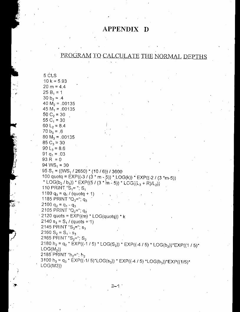
APPENDIX D

:PROGRAM ill CALCULATE THE NORMAL DE:PTHS

5 Cl810k=59320 m = 4.425 B1 = 130 b2 = .440 M2 = .0013545 M1 = .0013550 C2 = 3055 C1 = 3060 l2 = 8.470 b3 = .680 M3 = .0013585 C3 "' 3090 l3 = 8.691 q1 = .0393 R = 094 W81 = 30.9581 = ((W81 12650) * (10 16)) 13600

• I •

100 qualq = EXP((-31 (3 * m - 5)) *LOG(k)) * EXP((-21 (3 *m-5))* lOG(b21 b3)) * EXP((51 (3 * 1m - 5)) * LOG((I_3 .;. R)/L

2))

110 PRINT "81= "; 811180 q3 = q1 I (qualq + 1)1185 PRINT "03="; q32100 q2 = q 1- q32105 PRINT "02="; q2

. 2120 quaIs = EXP((m) * lOG(qualq)) * k2140 S3 = 811 (quaIs +'1)2145 PRINT "83="; S3216082 = 81- S32165 PRINT "82="; 822180 h2 = q2 * EXP((-1/5) * lOG(82)) * EXP((-4/5) * lOG(b2))*EXP((1/5)*lOG(M2))

2185 PRINT "h2="; h2

3100 h3 = q3 * EXP((-1/5)*lOG(s3)) * EXP((-4/5) *lOG(b3))*EXP((1/5)*lOG(M3))

D-1 '

3105 PRINT "h3="; h3,3120 i2 = (1 I q2) * EXP((3/5) * LOG(S2)) * EXP((2/5) *LOG(b2)) * EXP((-3 I 5) * LOG(M2)) * EXP((-2) * LOG(C2))3125 PRINT "i2="; 123140 i3= (1 I q3) * EXP((315) * LOG(S3)) * EXP((2/5) *LOG(b3)) * EXP((-3/5) * LOG(M3)) * EXP((-2) * LOG(C3))3145 PRINT "i3="; 133160 u2= q2 I (b2,* h2)3170 u3 = q31 (b3 * h3)3180 PRINT "U2=";U24100 PRINT "u3="; u34120 PRINT "Delta h=";4130 IF R <> 0 THEN PRINT (13 * R) ELSE PRINT "0"4140 REM if delta h larger then zero then the water level inbranch 3 is higher.4150 PRINT "02/03="; quatq4160 PRINT "SiS3="; quats'4180 h1= q1 * EXP((-1 15) * LOG(S1)) * EXP((-4/5) *LOG(B1)) * EXP((1 15) * LOG(M1))4190 '1 = (1 I q1) * EXP((3/5) * LOG(S1)) * EXP((2 15) *LOG(B1)) * EXP((-3/5) * LOG(M1)) * EXP((-2) * LOG(C1))4200 PRINT "h1 = "; h14210 PRINT"i1 ="; i14220 U1= q11 (h1 *.1)4230 PRINT "U1= "; u1END

D-2

, ,