
18 Machine Learning Radial Basis Function Networks Forward Heuristics
167
Neural Networks Radial Basis Function Networks - Forward Heuristics Andres Mendez-Vazquez December 10, 2015 1 / 58
-
Upload
andres-mendez-vazquez -
Category
Engineering
-
view
229 -
download
0
Transcript of 18 Machine Learning Radial Basis Function Networks Forward Heuristics

Neural NetworksRadial Basis Function Networks - Forward Heuristics
Andres Mendez-Vazquez
December 10, 2015
1 / 58

Outline
1 Predicting Variance of w and the output dThe Variance MatrixSelecting Regularization Parameter
2 How many dimensions?How many dimensions?
3 Forward Selection AlgorithmsIntroductionIncremental OperationsComplexity ComparisonAdding Basis Function Under RegularizationRemoving an Old Basis Function under RegularizationA Possible Forward Algorithm
2 / 58

Outline
1 Predicting Variance of w and the output dThe Variance MatrixSelecting Regularization Parameter
2 How many dimensions?How many dimensions?
3 Forward Selection AlgorithmsIntroductionIncremental OperationsComplexity ComparisonAdding Basis Function Under RegularizationRemoving an Old Basis Function under RegularizationA Possible Forward Algorithm
3 / 58
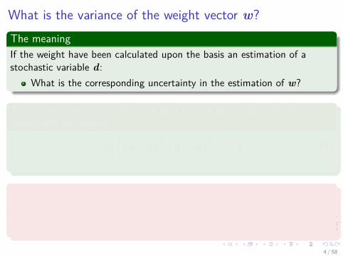
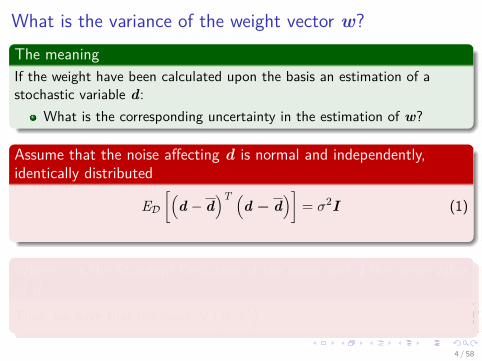
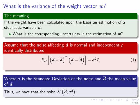
What is the variance of the weight vector w?The meaningIf the weight have been calculated upon the basis an estimation of astochastic variable d:
What is the corresponding uncertainty in the estimation of w?
Assume that the noise affecting d is normal and independently,identically distributed
ED[(
d − d)T (
d − d)]
= σ2I (1)
Where σ is the Standard Deviation of the noise and d the mean valueof dThus, we have that the noise N
(d, σ2
).
4 / 58

Remember
We are using a linear model
f (xi) =d1∑
j=1wjφj (xi) (2)
Thus, solving the error under regularization
w =[ΦTΦ + Λ
]−1ΦTd (3)
5 / 58

Remember
We are using a linear model
f (xi) =d1∑
j=1wjφj (xi) (2)
Thus, solving the error under regularization
w =[ΦTΦ + Λ
]−1ΦTd (3)
5 / 58

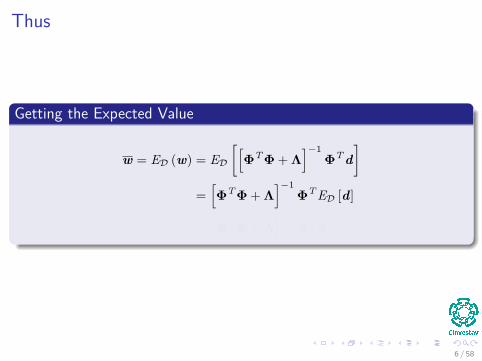
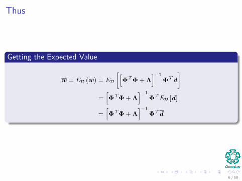
Thus
Getting the Expected Value
w = ED (w) = ED[[
ΦTΦ + Λ]−1
ΦTd]
=[ΦTΦ + Λ
]−1ΦTED [d]
=[ΦTΦ + Λ
]−1ΦTd
6 / 58
Thus
Getting the Expected Value
w = ED (w) = ED[[
ΦTΦ + Λ]−1
ΦTd]
=[ΦTΦ + Λ
]−1ΦTED [d]
=[ΦTΦ + Λ
]−1ΦTd
6 / 58
Thus
Getting the Expected Value
w = ED (w) = ED[[
ΦTΦ + Λ]−1
ΦTd]
=[ΦTΦ + Λ
]−1ΦTED [d]
=[ΦTΦ + Λ
]−1ΦTd
6 / 58

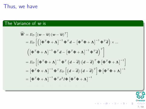
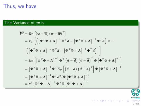
Thus, we have
The Variance of w is
W = ED[(w − w) (w − w)T]
= ED[([
ΦT Φ + Λ]−1 ΦT d −
[ΦT Φ + Λ
]−1 ΦT d)
× ...([ΦT Φ + Λ
]−1 ΦT d −[ΦT Φ + Λ
]−1 ΦT d)T]
= ED[[
ΦT Φ + Λ]−1 ΦT (d − d
) (d − d
)T Φ[ΦT Φ + Λ
]−1]
=[ΦT Φ + Λ
]−1 ΦT ED[(
d − d) (
d − d)T]
Φ[ΦT Φ + Λ
]−1
=[ΦT Φ + Λ
]−1 ΦTσ2IΦ[ΦT Φ + Λ
]−1
= σ2 [ΦT Φ + Λ]−1 ΦT Φ
[ΦT Φ + Λ
]−1
7 / 58

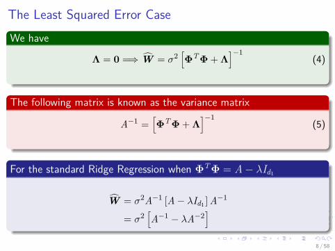
The Least Squared Error CaseWe have
Λ = 0 =⇒ W = σ2[ΦTΦ + Λ
]−1(4)
The following matrix is known as the variance matrix
A−1 =[ΦTΦ + Λ
]−1(5)
For the standard Ridge Regression when ΦTΦ = A− λId1
W = σ2A−1 [A− λId1 ] A−1
= σ2[A−1 − λA−2
]8 / 58

The Least Squared Error CaseWe have
Λ = 0 =⇒ W = σ2[ΦTΦ + Λ
]−1(4)
The following matrix is known as the variance matrix
A−1 =[ΦTΦ + Λ
]−1(5)
For the standard Ridge Regression when ΦTΦ = A− λId1
W = σ2A−1 [A− λId1 ] A−1
= σ2[A−1 − λA−2
]8 / 58

The Least Squared Error CaseWe have
Λ = 0 =⇒ W = σ2[ΦTΦ + Λ
]−1(4)
The following matrix is known as the variance matrix
A−1 =[ΦTΦ + Λ
]−1(5)
For the standard Ridge Regression when ΦTΦ = A− λId1
W = σ2A−1 [A− λId1 ] A−1
= σ2[A−1 − λA−2
]8 / 58
The Least Squared Error CaseWe have
Λ = 0 =⇒ W = σ2[ΦTΦ + Λ
]−1(4)
The following matrix is known as the variance matrix
A−1 =[ΦTΦ + Λ
]−1(5)
For the standard Ridge Regression when ΦTΦ = A− λId1
W = σ2A−1 [A− λId1 ] A−1
= σ2[A−1 − λA−2
]8 / 58
Outline
1 Predicting Variance of w and the output dThe Variance MatrixSelecting Regularization Parameter
2 How many dimensions?How many dimensions?
3 Forward Selection AlgorithmsIntroductionIncremental OperationsComplexity ComparisonAdding Basis Function Under RegularizationRemoving an Old Basis Function under RegularizationA Possible Forward Algorithm
9 / 58
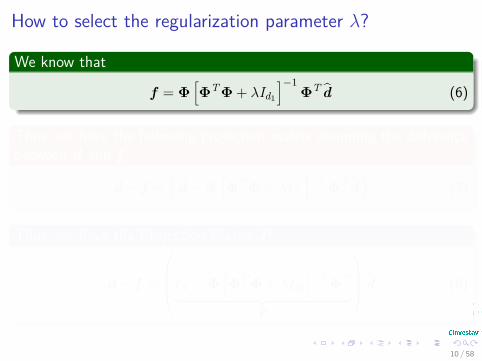
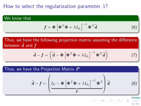
How to select the regularization parameter λ?
We know that
f = Φ[ΦTΦ + λId1
]−1ΦT d (6)
Thus, we have the following projection matrix assuming the differencebetween d and f
d − f =(
d −Φ[ΦTΦ + λId1
]−1ΦT d
)(7)
Thus, we have tha Projection Matrix P
d − f =
IN −Φ[ΦTΦ + λId1
]−1ΦT︸ ︷︷ ︸
P
d (8)
10 / 58

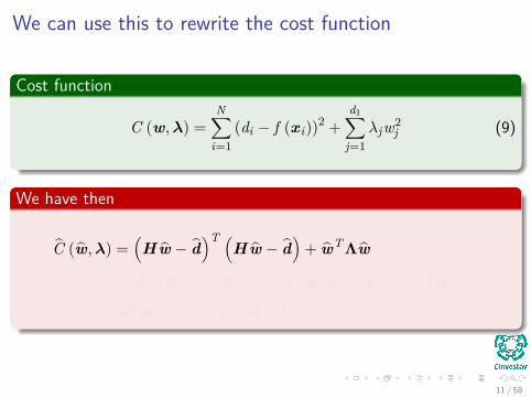
We can use this to rewrite the cost function
Cost function
C (w,λ) =N∑
i=1(di − f (xi))2 +
d1∑j=1
λjw2j (9)
We have then
C (w,λ) =(Hw − d
)T (Hw − d
)+ wTΛw
= dT (Φ [A]−1 ΦT − Id1
) (Φ [A]−1 ΦT − Id1
)d + ...
dTΦ [A]−1 Λ [A]−1 ΦT d
11 / 58
We can use this to rewrite the cost function
Cost function
C (w,λ) =N∑
i=1(di − f (xi))2 +
d1∑j=1
λjw2j (9)
We have then
C (w,λ) =(Hw − d
)T (Hw − d
)+ wTΛw
= dT (Φ [A]−1 ΦT − Id1
) (Φ [A]−1 ΦT − Id1
)d + ...
dTΦ [A]−1 Λ [A]−1 ΦT d
11 / 58

We can use this to rewrite the cost function
Cost function
C (w,λ) =N∑
i=1(di − f (xi))2 +
d1∑j=1
λjw2j (9)
We have then
C (w,λ) =(Hw − d
)T (Hw − d
)+ wTΛw
= dT (Φ [A]−1 ΦT − Id1
) (Φ [A]−1 ΦT − Id1
)d + ...
dTΦ [A]−1 Λ [A]−1 ΦT d
11 / 58

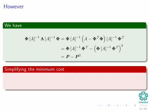
However
We have
Φ [A]−1 Λ [A]−1 Φ = Φ [A]−1(A−ΦTΦ
)[A]−1 ΦT
= Φ [A]−1 ΦT −(Φ [A]−1 ΦT
)2
= P −P2
Simplifying the minimum cost
C (w,λ) = dT P2 d+ dT (P −P2)
d = dT Pd (10)
12 / 58

However
We have
Φ [A]−1 Λ [A]−1 Φ = Φ [A]−1(A−ΦTΦ
)[A]−1 ΦT
= Φ [A]−1 ΦT −(Φ [A]−1 ΦT
)2
= P −P2
Simplifying the minimum cost
C (w,λ) = dT P2 d+ dT (P −P2)
d = dT Pd (10)
12 / 58
However
We have
Φ [A]−1 Λ [A]−1 Φ = Φ [A]−1(A−ΦTΦ
)[A]−1 ΦT
= Φ [A]−1 ΦT −(Φ [A]−1 ΦT
)2
= P −P2
Simplifying the minimum cost
C (w,λ) = dT P2 d+ dT (P −P2)
d = dT Pd (10)
12 / 58

However
We have
Φ [A]−1 Λ [A]−1 Φ = Φ [A]−1(A−ΦTΦ
)[A]−1 ΦT
= Φ [A]−1 ΦT −(Φ [A]−1 ΦT
)2
= P −P2
Simplifying the minimum cost
C (w,λ) = dT P2 d+ dT (P −P2)
d = dT Pd (10)
12 / 58
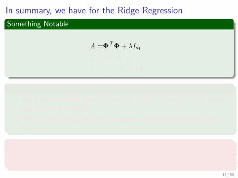
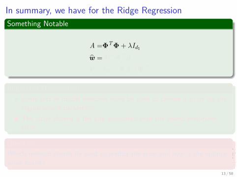
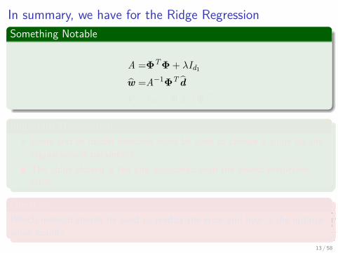
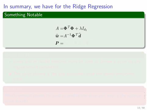
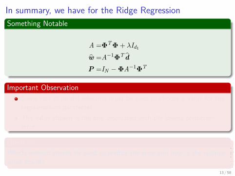
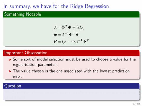
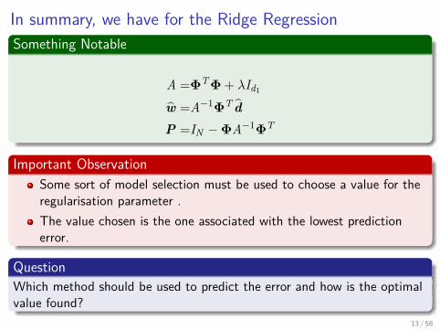
In summary, we have for the Ridge RegressionSomething Notable
A =ΦTΦ + λId1
w =A−1ΦT dP =IN −ΦA−1ΦT
Important ObservationSome sort of model selection must be used to choose a value for theregularisation parameter .The value chosen is the one associated with the lowest predictionerror.
QuestionWhich method should be used to predict the error and how is the optimalvalue found?
13 / 58

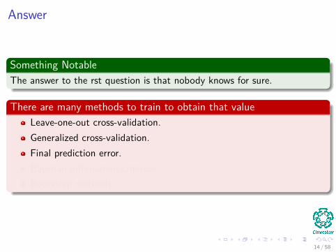
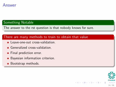
Answer
Something NotableThe answer to the rst question is that nobody knows for sure.
There are many methods to train to obtain that valueLeave-one-out cross-validation.Generalized cross-validation.Final prediction error.Bayesian information criterion.Bootstrap methods.
14 / 58
Answer
Something NotableThe answer to the rst question is that nobody knows for sure.
There are many methods to train to obtain that valueLeave-one-out cross-validation.Generalized cross-validation.Final prediction error.Bayesian information criterion.Bootstrap methods.
14 / 58
Answer
Something NotableThe answer to the rst question is that nobody knows for sure.
There are many methods to train to obtain that valueLeave-one-out cross-validation.Generalized cross-validation.Final prediction error.Bayesian information criterion.Bootstrap methods.
14 / 58
Answer
Something NotableThe answer to the rst question is that nobody knows for sure.
There are many methods to train to obtain that valueLeave-one-out cross-validation.Generalized cross-validation.Final prediction error.Bayesian information criterion.Bootstrap methods.
14 / 58

Answer
Something NotableThe answer to the rst question is that nobody knows for sure.
There are many methods to train to obtain that valueLeave-one-out cross-validation.Generalized cross-validation.Final prediction error.Bayesian information criterion.Bootstrap methods.
14 / 58
Answer
Something NotableThe answer to the rst question is that nobody knows for sure.
There are many methods to train to obtain that valueLeave-one-out cross-validation.Generalized cross-validation.Final prediction error.Bayesian information criterion.Bootstrap methods.
14 / 58
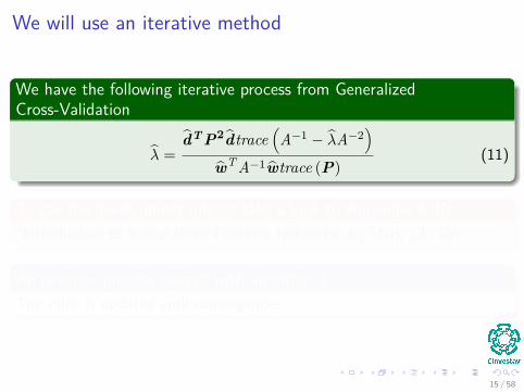
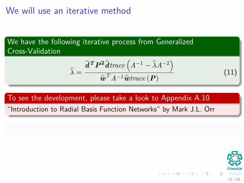
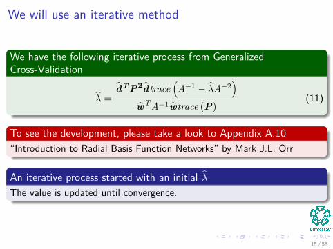
We will use an iterative method
We have the following iterative process from GeneralizedCross-Validation
λ =dTP2dtrace
(A−1 − λA−2
)wT A−1wtrace (P)
(11)
To see the development, please take a look to Appendix A.10“Introduction to Radial Basis Function Networks” by Mark J.L. Orr
An iterative process started with an initial λ
The value is updated until convergence.
15 / 58
Outline
1 Predicting Variance of w and the output dThe Variance MatrixSelecting Regularization Parameter
2 How many dimensions?How many dimensions?
3 Forward Selection AlgorithmsIntroductionIncremental OperationsComplexity ComparisonAdding Basis Function Under RegularizationRemoving an Old Basis Function under RegularizationA Possible Forward Algorithm
16 / 58
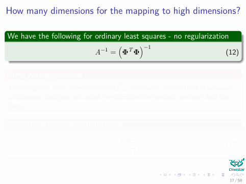
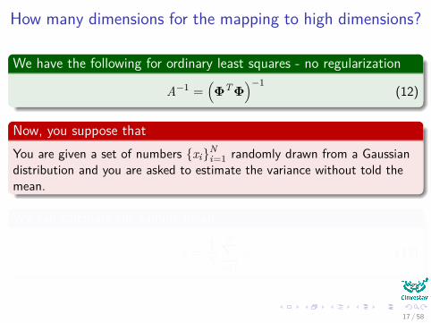
How many dimensions for the mapping to high dimensions?
We have the following for ordinary least squares - no regularization
A−1 =(ΦTΦ
)−1(12)
Now, you suppose thatYou are given a set of numbers {xi}Ni=1 randomly drawn from a Gaussiandistribution and you are asked to estimate the variance without told themean.
We can calculate the sample mean
x = 1N
N∑i=1
xi (13)
17 / 58

Thus
This allows to calculate the sample variance
σ2 = 1N − 1
N∑i=1
(xi − x)2 (14)
Problem, from Where the parameter N − 1 comes from?It comes from the fact that the parameter x is fitting the noise.
The system has N degrees of freedomThus the underestimation of the variance is restored by reducing theremaining degrees of freedom by one.
18 / 58

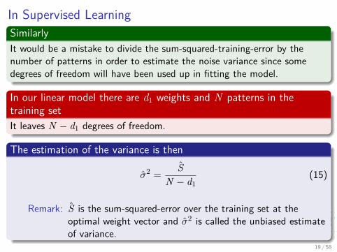
In Supervised LearningSimilarlyIt would be a mistake to divide the sum-squared-training-error by thenumber of patterns in order to estimate the noise variance since somedegrees of freedom will have been used up in fitting the model.
In our linear model there are d1 weights and N patterns in thetraining setIt leaves N − d1 degrees of freedom.
The estimation of the variance is then
σ2 = SN − d1
(15)
Remark: S is the sum-squared-error over the training set at theoptimal weight vector and σ2 is called the unbiased estimateof variance.
19 / 58
First, standard least squared error
Although there is still d1 weights in the modelThe effective number of parameters(John Moody), γ, is less than d1and it depends on the size of the regularization parameters.
We have the following (Moody and MacKay)
γ = N − trace (P) (16)
20 / 58

First, standard least squared error
Although there is still d1 weights in the modelThe effective number of parameters(John Moody), γ, is less than d1and it depends on the size of the regularization parameters.
We have the following (Moody and MacKay)
γ = N − trace (P) (16)
20 / 58

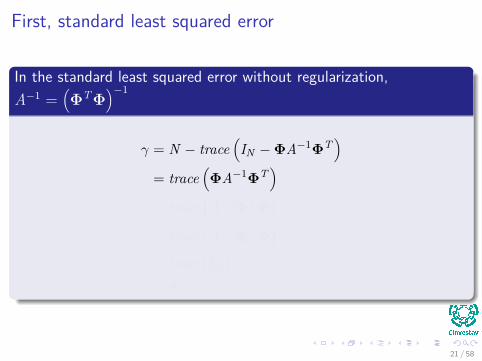
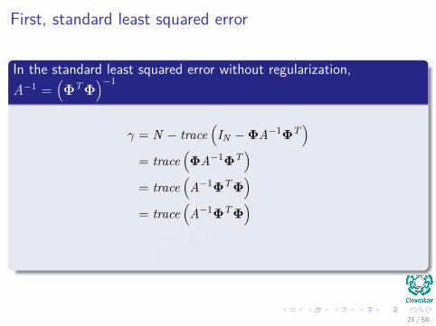
First, standard least squared error
In the standard least squared error without regularization,A−1 =
(ΦTΦ
)−1
γ = N − trace(IN −ΦA−1ΦT
)= trace
(ΦA−1ΦT
)= trace
(A−1ΦTΦ
)= trace
(A−1ΦTΦ
)= trace (Id1)= d1
21 / 58
First, standard least squared error
In the standard least squared error without regularization,A−1 =
(ΦTΦ
)−1
γ = N − trace(IN −ΦA−1ΦT
)= trace
(ΦA−1ΦT
)= trace
(A−1ΦTΦ
)= trace
(A−1ΦTΦ
)= trace (Id1)= d1
21 / 58

First, standard least squared error
In the standard least squared error without regularization,A−1 =
(ΦTΦ
)−1
γ = N − trace(IN −ΦA−1ΦT
)= trace
(ΦA−1ΦT
)= trace
(A−1ΦTΦ
)= trace
(A−1ΦTΦ
)= trace (Id1)= d1
21 / 58
First, standard least squared error
In the standard least squared error without regularization,A−1 =
(ΦTΦ
)−1
γ = N − trace(IN −ΦA−1ΦT
)= trace
(ΦA−1ΦT
)= trace
(A−1ΦTΦ
)= trace
(A−1ΦTΦ
)= trace (Id1)= d1
21 / 58

First, standard least squared error
In the standard least squared error without regularization,A−1 =
(ΦTΦ
)−1
γ = N − trace(IN −ΦA−1ΦT
)= trace
(ΦA−1ΦT
)= trace
(A−1ΦTΦ
)= trace
(A−1ΦTΦ
)= trace (Id1)= d1
21 / 58

First, standard least squared error
In the standard least squared error without regularization,A−1 =
(ΦTΦ
)−1
γ = N − trace(IN −ΦA−1ΦT
)= trace
(ΦA−1ΦT
)= trace
(A−1ΦTΦ
)= trace
(A−1ΦTΦ
)= trace (Id1)= d1
21 / 58
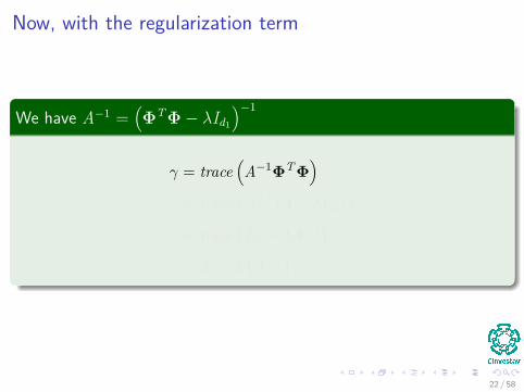
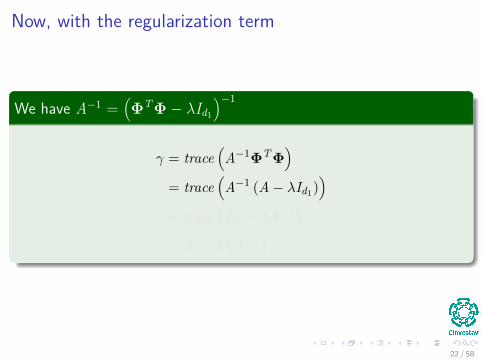
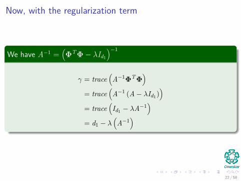
Now, with the regularization term
We have A−1 =(ΦTΦ− λId1
)−1
γ = trace(A−1ΦTΦ
)= trace
(A−1 (A− λId1)
)= trace
(Id1 − λA−1
)= d1 − λ
(A−1
)
22 / 58
Now, with the regularization term
We have A−1 =(ΦTΦ− λId1
)−1
γ = trace(A−1ΦTΦ
)= trace
(A−1 (A− λId1)
)= trace
(Id1 − λA−1
)= d1 − λ
(A−1
)
22 / 58

Now, with the regularization term
We have A−1 =(ΦTΦ− λId1
)−1
γ = trace(A−1ΦTΦ
)= trace
(A−1 (A− λId1)
)= trace
(Id1 − λA−1
)= d1 − λ
(A−1
)
22 / 58
Now, with the regularization term
We have A−1 =(ΦTΦ− λId1
)−1
γ = trace(A−1ΦTΦ
)= trace
(A−1 (A− λId1)
)= trace
(Id1 − λA−1
)= d1 − λ
(A−1
)
22 / 58

Now
If the eigenvalues of the matrix ΦTΦ are {µj}d1j=1
γ = d1 − λtrace(A−1
)= d1 − λ
d1∑i=1
1λ+ µj
=d1∑
i=1
µjλ+ µj
23 / 58

Now
If the eigenvalues of the matrix ΦTΦ are {µj}d1j=1
γ = d1 − λtrace(A−1
)= d1 − λ
d1∑i=1
1λ+ µj
=d1∑
i=1
µjλ+ µj
23 / 58

Now
If the eigenvalues of the matrix ΦTΦ are {µj}d1j=1
γ = d1 − λtrace(A−1
)= d1 − λ
d1∑i=1
1λ+ µj
=d1∑
i=1
µjλ+ µj
23 / 58
Outline
1 Predicting Variance of w and the output dThe Variance MatrixSelecting Regularization Parameter
2 How many dimensions?How many dimensions?
3 Forward Selection AlgorithmsIntroductionIncremental OperationsComplexity ComparisonAdding Basis Function Under RegularizationRemoving an Old Basis Function under RegularizationA Possible Forward Algorithm
24 / 58
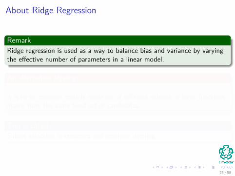
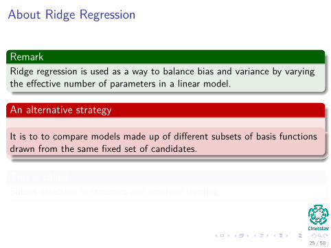
About Ridge Regression
RemarkRidge regression is used as a way to balance bias and variance by varyingthe effective number of parameters in a linear model.
An alternative strategy
It is to to compare models made up of different subsets of basis functionsdrawn from the same fixed set of candidates.
This is calledSubset selection in statistics and machine learning.
25 / 58

Problem
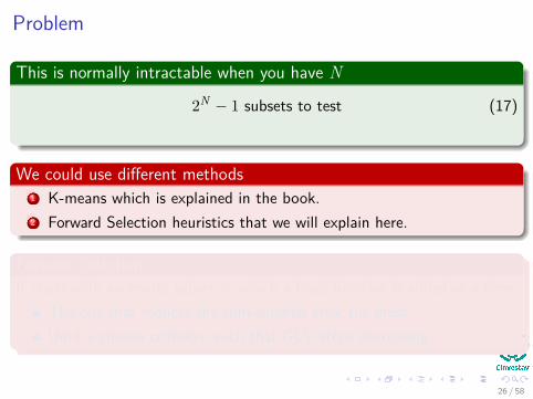
This is normally intractable when you have N
2N − 1 subsets to test (17)
We could use different methods1 K-means which is explained in the book.2 Forward Selection heuristics that we will explain here.
Forward SelectionIt starts with an empty subset to which a basis function is added at a time:
The one that reduces the sum-squared error the most.Until a chosen criterion, such that GCV stops decreasing.
26 / 58

Problem
This is normally intractable when you have N
2N − 1 subsets to test (17)
We could use different methods1 K-means which is explained in the book.2 Forward Selection heuristics that we will explain here.
Forward SelectionIt starts with an empty subset to which a basis function is added at a time:
The one that reduces the sum-squared error the most.Until a chosen criterion, such that GCV stops decreasing.
26 / 58
Subset Selection Vs. Optimization
Classic Neural Network OptimizationIt involves the optimization, by gradient descent, of a nonlinearsum-squared-error surface in a high-dimensional space defined by thenetwork parameters.
In specific in RBFThe network parameters are the centers, sizes and hidden-to-outputweights.
27 / 58

Subset Selection Vs. Optimization
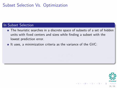
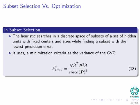
In Subset SelectionThe heuristic searches in a discrete space of subsets of a set of hiddenunits with fixed centers and sizes while finding a subset with thelowest prediction error.It uses, a minimization criteria as the variance of the GVC:
σ2GCV = N dT P2d
trace (P)2 (18)
28 / 58
Subset Selection Vs. Optimization
In Subset SelectionThe heuristic searches in a discrete space of subsets of a set of hiddenunits with fixed centers and sizes while finding a subset with thelowest prediction error.It uses, a minimization criteria as the variance of the GVC:
σ2GCV = N dT P2d
trace (P)2 (18)
28 / 58
In addition
Hidden-to-Output WeightsThey are not selected, they are slaved to the centers and sizes of thechosen subset.
Forward selection is a non-linear type of heuristic with the followingadvantages
There is no need to fix the number of hidden units in advance.The model selection criteria are tractable.The computational requirements are relatively low.
29 / 58

Thus, under the classic least squared error
Something NotableIn forward selection each step involves growing the network by one basisfunction.
ThereforeAdding a new basis function is one of the incremental operations by usingthe equation
Pd1+1 = Pd1 −Pd1φjφ
Tj Pd1
φTj Pd1φj
(19)
30 / 58
Thus, under the classic least squared error
Something NotableIn forward selection each step involves growing the network by one basisfunction.
ThereforeAdding a new basis function is one of the incremental operations by usingthe equation
Pd1+1 = Pd1 −Pd1φjφ
Tj Pd1
φTj Pd1φj
(19)
30 / 58

Thus
WherePm+1 is the succeeding projection matrix if the J -th member of theset is added.Pm the projection matrix for the m−hidden units.
The vectors{
φj
}N
j=1are the column vectors of the matrix Φ with
N � d1.
31 / 58
Thus
WherePm+1 is the succeeding projection matrix if the J -th member of theset is added.Pm the projection matrix for the m−hidden units.
The vectors{
φj
}N
j=1are the column vectors of the matrix Φ with
N � d1.
31 / 58
Thus
WherePm+1 is the succeeding projection matrix if the J -th member of theset is added.Pm the projection matrix for the m−hidden units.
The vectors{
φj
}N
j=1are the column vectors of the matrix Φ with
N � d1.
31 / 58
Thus
We have that
ΦN = [φ1 φ2 ... φN ] (20)
If we take in account all the possible centers given by all the basis
32 / 58

Outline
1 Predicting Variance of w and the output dThe Variance MatrixSelecting Regularization Parameter
2 How many dimensions?How many dimensions?
3 Forward Selection AlgorithmsIntroductionIncremental OperationsComplexity ComparisonAdding Basis Function Under RegularizationRemoving an Old Basis Function under RegularizationA Possible Forward Algorithm
33 / 58

What are we going to do?
This is what we want to do1 Adding a new basis function2 Removing an old basis function
34 / 58

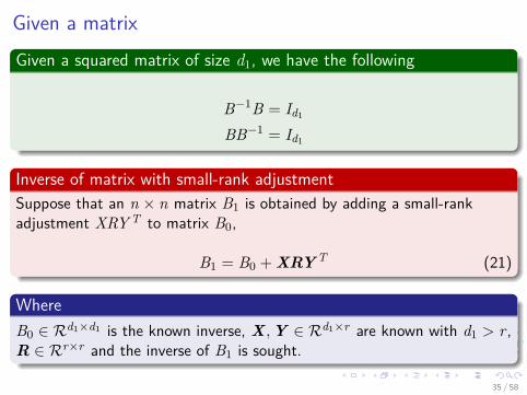
Given a matrixGiven a squared matrix of size d1, we have the following
B−1B = Id1
BB−1 = Id1
Inverse of matrix with small-rank adjustmentSuppose that an n × n matrix B1 is obtained by adding a small-rankadjustment XRY T to matrix B0,
B1 = B0 + XRY T (21)
WhereB0 ∈ Rd1×d1 is the known inverse, X ,Y ∈ Rd1×r are known with d1 > r ,R ∈ Rr×r and the inverse of B1 is sought.
35 / 58

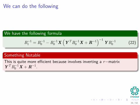
We can do the following
We have the following formula
B−11 = B−1
0 − B−10 X
(Y T B−1
0 X + R−1)−1
Y B−10 (22)
Something NotableThis is quite more efficient because involves inverting a r−matrixY T B−1
0 X + R−1.
36 / 58
We can do the following
We have the following formula
B−11 = B−1
0 − B−10 X
(Y T B−1
0 X + R−1)−1
Y B−10 (22)
Something NotableThis is quite more efficient because involves inverting a r−matrixY T B−1
0 X + R−1.
36 / 58
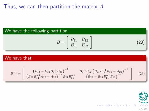
Thus, we can then partition the matrix A
We have the following partition
B =[
B11 B12B21 B22
](23)
We have that
B−1 =
[ (B11 − B12B−1
22 B21)−1
B−111 B12
(B21B−1
11 B12 −A22)−1(
B21B−111 A12 −A22
)−1B21B−1
11(
B22 − B21B−111 B12
)−1
](24)
37 / 58
Thus, we can then partition the matrix A
We have the following partition
B =[
B11 B12B21 B22
](23)
We have that
B−1 =
[ (B11 − B12B−1
22 B21)−1
B−111 B12
(B21B−1
11 B12 −A22)−1(
B21B−111 A12 −A22
)−1B21B−1
11(
B22 − B21B−111 B12
)−1
](24)
37 / 58

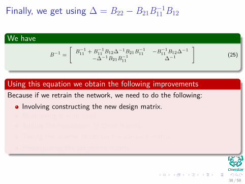
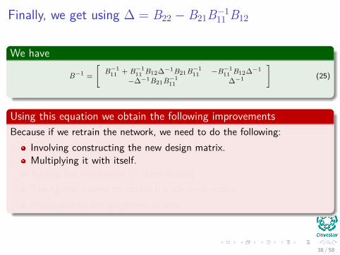
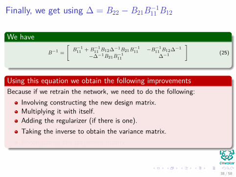
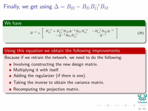
Finally, we get using ∆ = B22 − B21B−111 B12
We have
B−1 =[
B−111 + B−1
11 B12∆−1B21B−111 −B−1
11 B12∆−1
−∆−1B21B−111 ∆−1
](25)
Using this equation we obtain the following improvementsBecause if we retrain the network, we need to do the following:
Involving constructing the new design matrix.Multiplying it with itself.Adding the regularizer (if there is one).Taking the inverse to obtain the variance matrix.Recomputing the projection matrix.
38 / 58

Outline
1 Predicting Variance of w and the output dThe Variance MatrixSelecting Regularization Parameter
2 How many dimensions?How many dimensions?
3 Forward Selection AlgorithmsIntroductionIncremental OperationsComplexity ComparisonAdding Basis Function Under RegularizationRemoving an Old Basis Function under RegularizationA Possible Forward Algorithm
39 / 58

Complexity of calculation of P
We have the following approximate number of multiplicationsOperation Completely Retrain Using Operation
Add a new basis d31 + Nd2
1 + N 2d1 N 2
Remove an old basis d31 + Nd2
1 + N 2d1 N 2
Add a new pattern d31 + Nd2
1 + N 2d1 2d21 + d1N + N 2
Remove an old pattern d31 + Nd2
1 + N 2d1 2d21 + d1N + N 2
40 / 58

Outline
1 Predicting Variance of w and the output dThe Variance MatrixSelecting Regularization Parameter
2 How many dimensions?How many dimensions?
3 Forward Selection AlgorithmsIntroductionIncremental OperationsComplexity ComparisonAdding Basis Function Under RegularizationRemoving an Old Basis Function under RegularizationA Possible Forward Algorithm
41 / 58

Adding a Basis Function
We do the followingIf the J−th basis function is chosen then φj is appended to the lastcolumn of Φd1 and renamed m + 1.
Thus, incrementing to the new matrix
Φd1+1 =[Φd1 φd1+1
](26)
42 / 58

Adding a Basis Function
We do the followingIf the J−th basis function is chosen then φj is appended to the lastcolumn of Φd1 and renamed m + 1.
Thus, incrementing to the new matrix
Φd1+1 =[Φd1 φd1+1
](26)
42 / 58

Where
We have that
φd1+1 =
φd1+1 (x1)φd1+1 (x2)
...φd1+1 (xN )
(27)
43 / 58
Using our variance matrix
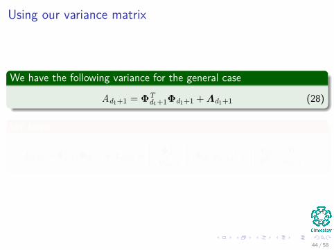
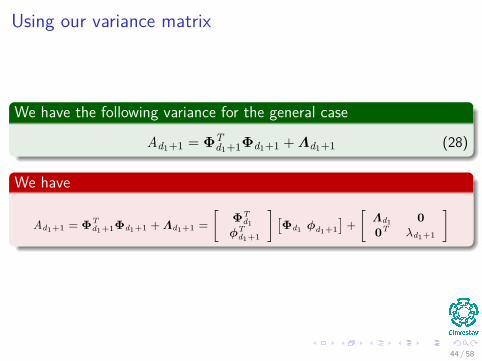
We have the following variance for the general case
Ad1+1 = ΦTd1+1Φd1+1 + Λd1+1 (28)
We have
Ad1+1 = ΦTd1+1Φd1+1 + Λd1+1 =
[ΦT
d1φT
d1+1
] [Φd1 φd1+1
]+[
Λd1 00T λd1+1
]
44 / 58
Using our variance matrix
We have the following variance for the general case
Ad1+1 = ΦTd1+1Φd1+1 + Λd1+1 (28)
We have
Ad1+1 = ΦTd1+1Φd1+1 + Λd1+1 =
[ΦT
d1φT
d1+1
] [Φd1 φd1+1
]+[
Λd1 00T λd1+1
]
44 / 58
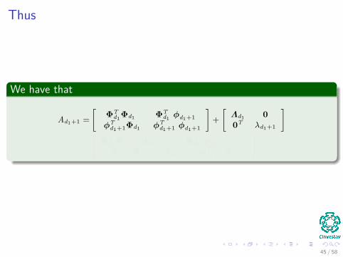
Thus
We have that
Ad1+1 =[
ΦTd1 Φd1 ΦT
d1 φd1+1φT
d1+1Φd1 φTd1+1 φd1+1
]+[
Λd1 00T λd1+1
]=[
ΦTd1 Φd1 + Λd1 ΦT
d1 φd1+1φT
d1+1Φd1 λd1+1 + φTd1+1 φd1+1
]
45 / 58

Thus
We have that
Ad1+1 =[
ΦTd1 Φd1 ΦT
d1 φd1+1φT
d1+1Φd1 φTd1+1 φd1+1
]+[
Λd1 00T λd1+1
]=[
ΦTd1 Φd1 + Λd1 ΦT
d1 φd1+1φT
d1+1Φd1 λd1+1 + φTd1+1 φd1+1
]
45 / 58

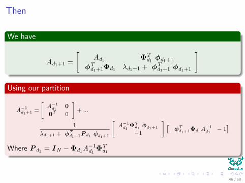
Then
We have
Ad1+1 =[
Ad1 ΦTd1 φd1+1
φTd1+1Φd1 λd1+1 + φT
d1+1 φd1+1
]
Using our partition
A−1d1+1 =
[A−1
d10
0T 0
]+ ...
1λd1+1 + φT
d1+1Pd1 φd1+1
[A−1
d1ΦT
d1 φd1+1−1
] [φT
d1+1Φd1 A−1d1
− 1]
Where Pd1 = I N −Φd1A−1d1
ΦTd1
46 / 58

Then
We have
Ad1+1 =[
Ad1 ΦTd1 φd1+1
φTd1+1Φd1 λd1+1 + φT
d1+1 φd1+1
]
Using our partition
A−1d1+1 =
[A−1
d10
0T 0
]+ ...
1λd1+1 + φT
d1+1Pd1 φd1+1
[A−1
d1ΦT
d1 φd1+1−1
] [φT
d1+1Φd1 A−1d1
− 1]
Where Pd1 = I N −Φd1A−1d1
ΦTd1
46 / 58
Then
We have
Ad1+1 =[
Ad1 ΦTd1 φd1+1
φTd1+1Φd1 λd1+1 + φT
d1+1 φd1+1
]
Using our partition
A−1d1+1 =
[A−1
d10
0T 0
]+ ...
1λd1+1 + φT
d1+1Pd1 φd1+1
[A−1
d1ΦT
d1 φd1+1−1
] [φT
d1+1Φd1 A−1d1
− 1]
Where Pd1 = I N −Φd1A−1d1
ΦTd1
46 / 58
Finally
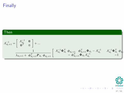
Then
A−1d1+1 =
[A−1
d10
0T 0
]+ ...
1λd1+1 + φT
d1+1Pd1 φd1+1
[A−1
d1ΦT
d1 φd1+1 φTd1+1Φd1 − A−1
d1A−1
d1ΦT
d1 φd1+1− φT
d1+1Φd1 A−1d1
−1
]
47 / 58

We have then that
We can use the previous result for A−1m+1
Pd1+1 =I N −Φd1+1A−1d1+1Φ
Td1+1
=Pd1 −Pd1 φd1+1 φT
d1+1Pd1
λd1+1 + φTd1+1Pd1 φd1+1
48 / 58

We have then that
We can use the previous result for A−1m+1
Pd1+1 =I N −Φd1+1A−1d1+1Φ
Td1+1
=Pd1 −Pd1 φd1+1 φT
d1+1Pd1
λd1+1 + φTd1+1Pd1 φd1+1
48 / 58

How do we select the new basis
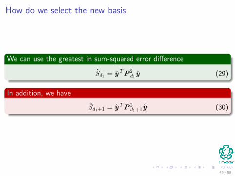
We can use the greatest in sum-squared error difference
Sd1 = yT P2d1 y (29)
In addition, we have
Sd1+1 = yT P2d1+1y (30)
49 / 58
How do we select the new basis
We can use the greatest in sum-squared error difference
Sd1 = yT P2d1 y (29)
In addition, we have
Sd1+1 = yT P2d1+1y (30)
49 / 58

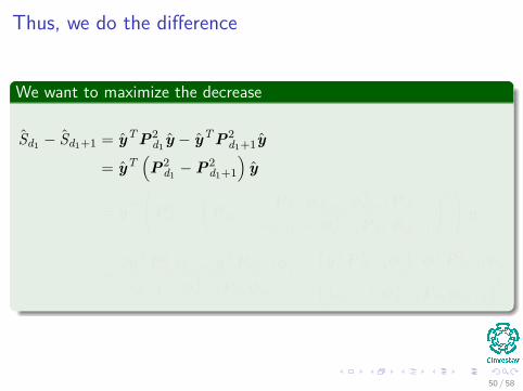
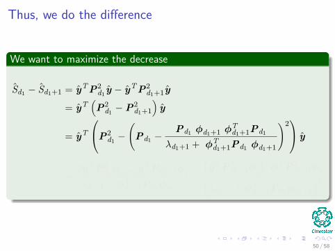
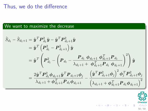
Thus, we do the difference
We want to maximize the decrease
Sd1 − Sd1+1 = yT P2d1 y − yT P2
d1+1y
= yT(P2
d1 −P2d1+1
)y
= yT
P2d1 −
(Pd1 −
Pd1 φd1+1 φTd1+1Pd1
λd1+1 + φTd1+1Pd1 φd1+1
)2 y
=2yT P2
d1φd1+1yT Pd1+1φj
λd1+1 + φTd1+1Pd1φd1+1
−
(yT P2
d1+1φj
)2φT
j P2d1+1φj(
λd1+1 + φTd1+1Pd1φd1+1
)2
50 / 58

An alternative is is to seek to maximize the decrease in thecost function
We have
Cd1 − Cd1+1 = yT Pd1 y − yT Pd1+1y
= yT Pd1 φd1+1 φTd1+1Pd1
λd1+1 + φTd1+1Pd1 φd1+1
y
=
(yT Pd1 φd1+1
)2
λd1+1 + φTd1+1Pd1 φd1+1
51 / 58

Outline
1 Predicting Variance of w and the output dThe Variance MatrixSelecting Regularization Parameter
2 How many dimensions?How many dimensions?
3 Forward Selection AlgorithmsIntroductionIncremental OperationsComplexity ComparisonAdding Basis Function Under RegularizationRemoving an Old Basis Function under RegularizationA Possible Forward Algorithm
52 / 58

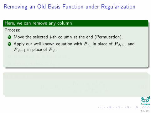
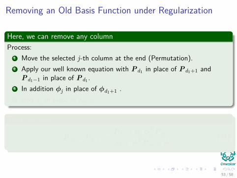
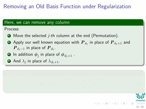
Removing an Old Basis Function under Regularization
Here, we can remove any columnProcess:
1 Move the selected j-th column at the end (Permutation).2 Apply our well known equation with Pd1 in place of Pd1+1 and
Pd1−1 in place of Pd1 .3 In addition φj in place of φd1+1 .4 And λj in place of λd1+1.
Thus, we have
Pd1 = Pd1−1 −Pd1−1 φj φT
j Pd1−1
λj + φTj Pd1−1 φj
(31)
53 / 58
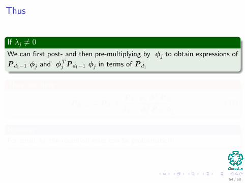
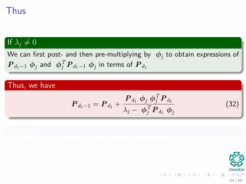
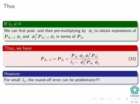
Thus
If λj 6= 0We can first post- and then pre-multiplying by φj to obtain expressions ofPd1−1 φj and φT
j Pd1−1 φj in terms of Pd1
Thus, we have
Pd1−1 = Pd1 +Pd1 φj φT
j Pd1
λj − φTj Pd1 φj
(32)
HoweverFor small λj , the round-off error can be problematic!!!
54 / 58
Thus
If λj 6= 0We can first post- and then pre-multiplying by φj to obtain expressions ofPd1−1 φj and φT
j Pd1−1 φj in terms of Pd1
Thus, we have
Pd1−1 = Pd1 +Pd1 φj φT
j Pd1
λj − φTj Pd1 φj
(32)
HoweverFor small λj , the round-off error can be problematic!!!
54 / 58
Thus
If λj 6= 0We can first post- and then pre-multiplying by φj to obtain expressions ofPd1−1 φj and φT
j Pd1−1 φj in terms of Pd1
Thus, we have
Pd1−1 = Pd1 +Pd1 φj φT
j Pd1
λj − φTj Pd1 φj
(32)
HoweverFor small λj , the round-off error can be problematic!!!
54 / 58
Outline
1 Predicting Variance of w and the output dThe Variance MatrixSelecting Regularization Parameter
2 How many dimensions?How many dimensions?
3 Forward Selection AlgorithmsIntroductionIncremental OperationsComplexity ComparisonAdding Basis Function Under RegularizationRemoving an Old Basis Function under RegularizationA Possible Forward Algorithm
55 / 58

Based in the previous ideas
We are ready for a basic algorithmHowever, this can be improved.
56 / 58
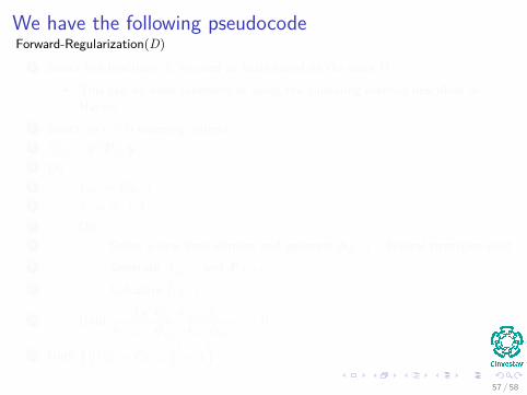
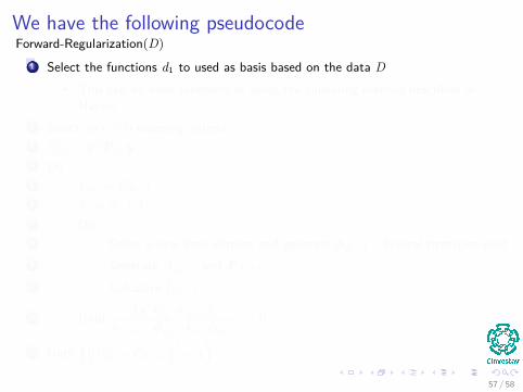
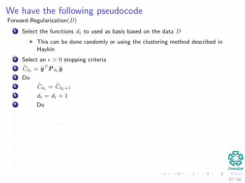
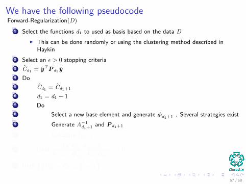
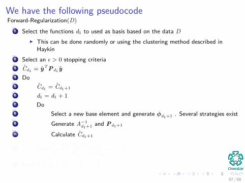
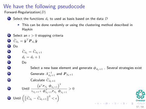
We have the following pseudocodeForward-Regularization(D)
1 Select the functions d1 to used as basis based on the data DI This can be done randomly or using the clustering method described in
Haykin2 Select an ε > 0 stopping criteria3 Cd1 = yT Pd1 y4 Do5 Cd1 = Cd1+1
6 d1 = d1 + 17 Do8 Select a new base element and generate φd1+1 . Several strategies exist9 Generate A−1
d1+1 and Pd1+1
10 Calculate Cd1+1
11 Until(
yT Pd1 φd1+1
)2
λd1+1+ φTd1+1Pd1 φd1+1
> 0
12 Until(∥∥Cd1 − Cd1+1
∥∥2< ε)
57 / 58
For more on this
Please Read the followingIntroduction to Radial Basis Function Networks by Mark J. L. Orr
And there is much moreLook At the book Bootstrap Methods and their Application by A. C.Davison and D. V. Hinkley
58 / 58

For more on this
Please Read the followingIntroduction to Radial Basis Function Networks by Mark J. L. Orr
And there is much moreLook At the book Bootstrap Methods and their Application by A. C.Davison and D. V. Hinkley
58 / 58