Radial basis functions - University of California, Davissaito/data/jim/buhmann-actanumerica.pdf ·...

Acta Numerica (2000), pp. 1–38 c© Cambridge University Press, 2000

Radial basis functions

M. D. BuhmannMathematical Institute,

Justus Liebig University,

35392 Giessen, Germany

E-mail: [email protected]

Radial basis function methods are modern ways to approximate multivariatefunctions, especially in the absence of grid data. They have been known,tested and analysed for several years now and many positive properties havebeen identified. This paper gives a selective but up-to-date survey of severalrecent developments that explains their usefulness from the theoretical pointof view and contributes useful new classes of radial basis function. We considerparticularly the new results on convergence rates of interpolation with radialbasis functions, as well as some of the various achievements on approximationon spheres, and the efficient numerical computation of interpolants for verylarge sets of data. Several examples of useful applications are stated at theend of the paper.

CONTENTS

1 Introduction 12 Convergence rates 53 Compact support 114 Iterative methods for implementation 165 Interpolation on spheres 256 Applications 28References 34

1. Introduction

There is a multitude of ways to approximate a function of many variables:multivariate polynomials, splines, tensor product methods, local methodsand global methods. All of these approaches have many advantages andsome disadvantages, but if the dimensionality of the problem (the numberof variables) is large, which is often the case in many applications from stat-istics to neural networks, our choice of methods is greatly reduced, unless

2 M. D. Buhmann

we resort solely to tensor product methods. In fact, sometimes we are givenscattered data, immediately excluding the use of tensor product methods.Also, tensor product methods in high dimensions always require many, of-ten too many data. In this situation, the method of choice is often a radialbasis function approach which is, incidentally, also highly useful in lower-dimensional problems and as an alternative to (piecewise) polynomials, be-cause of its excellent approximation properties; at any rate it is universallyapplicable independent of dimension.

In order to formulate the problem as we will see it in this review, let Ξbe a finite set of distinct points in R

n, which are traditionally called centresin radial basis function jargon, because our basis functions will be radiallysymmetric about these points. The goal of our work is to approximate anunknown function that is only given at those centres via a set of real numbersfξ, ξ ∈ Ξ. These are almost always interpreted as function evaluations ofsome smooth function f : R

n ⊃ Ω → R, so that fξ = f(ξ). Here, Ω is adomain in R

n. This point of view will allow us to measure conveniently theuniform approximation error between f and its approximant s. This errordepends on the choice of the approximant, on Ξ, on f , and in particular onits smoothness.

In order to approximate with s, which is usually by interpolation, wetake a univariate continuous function φ that is radialized by compositionwith the Euclidean norm on R

n, or a suitable replacement thereof whenwe are working on a sphere in n-dimensional Euclidean space, for instance.This φ : R+ → R is the radial basis function. Additionally, we take thegiven centres ξ from the given finite set Ξ of distinct points and use themsimultaneously for shifting the radial basis function and as interpolation(collocation) points. Therefore, our standard radial function approximantsnow have the form

s(x) =∑ξ∈Ξ

λξφ(‖x− ξ‖), x ∈ Rn, (1.1)

suitable adjustments being made when x is not from the whole space, andthe coefficient vector λ = (λξ)ξ∈Ξ is an element of R

Ξ. In many instances,particularly those that will interest us in Section 3, the interpolation re-quirements

s |Ξ= f |Ξ (1.2)

for given data f |Ξ lead to a positive definite interpolation matrix A =φ(‖ξ − ζ‖)ξ,ζ∈Ξ. In that case, we call the radial basis function ‘positivedefinite’ as well. If it is, the linear system of equations that comes from (1.1)and (1.2) and uses precisely that matrix A yields a unique coefficient vectorλ ∈ R

Ξ for the interpolant (1.1).All radial basis functions of Section 3 have this property of positive defin-

Radial basis functions 3

iteness, as does for instance the Gaussian radial basis function φ(r) = e−c2r2

for all positive parameters c and the inverse multiquadric function φ(r) =1/√r2 + c2.

However, in some instances such as the so-called thin-plate spline radialbasis function, the radial function φ is only conditionally positive definiteof some order k on R

n, say, a notion that we shall explain and use in thesubsequent section. Now, in this event, polynomials p(x) ∈ P

k−1n (x) of degree

k − 1 in n unknowns are augmented to the right-hand side of (1.1) so as torender the interpolation problem again uniquely solvable. Consequently wehave as approximant

s(x) =∑ξ∈Ξ

λξφ(‖x− ξ‖) + p(x), x ∈ Rn. (1.3)

Then the extra degrees of freedom are taken up by requiring that the coeffi-cient vector λ ∈ R

Ξ is orthogonal to the polynomial space Pk−1n (Ξ), that is,

all polynomials of total degree less than k in n variables restricted to Ξ:

RΞ 3 λ ⊥ P

k−1n (Ξ) ⇐⇒

∑ξ∈Ξ

λξq(ξ) = 0, ∀ q ∈ Pk−1n . (1.4)

In order to retain uniqueness, Ξ has to contain a Pk−1n -unisolvent subset in

this case. When k = 2, for instance, this means that the centre-set mustnot be a subset of a straight line. This is a requirement that can easily bemet in most cases.

The two probably best-known and most often applied radial basis func-tions are called multiquadrics and thin-plate splines, respectively. Theformer is, for a positive parameter c, φ(r) =

√r2 + c2 and the latter is

φ(r) = r2 log r, where in the second case (1.3) and (1.4) with k = 2 areapplied. The multiquadric is, subject to a sign change, conditionally posit-ive definite of order k = 1, but it turns out that the original interpolationproblem without augmentation by constants is also nonsingular because ofspecial properties of the multiquadric function (Micchelli 1986).

One more well-known example comes up when we set c = 0 in the mul-tiquadric example: then we have the so-called linear radial basis functionφ(r) = r which also gives a nonsingular interpolation problem without aug-mentation by constants. All these examples are useful for various forms ofinterpolation and approximation and they all allow this interpolation pro-cedure in all dimensions n and all sets of distinct centres, independently ofthe geometry of the points. In contrast to spline approximation in morethan one dimension, for instance, there is no triangulation or tessellation ofthe data points required, nor is there any restriction on the dimensionalityof the problem. We note, however, that these nonsingularity properties arestrictly linked to the fact that we use Euclidean norms; for p-norms with

4 M. D. Buhmann

p > 2, including p = ∞, or p = 1, singularity can occur in any dimensionfor unfortunate choices of data points ξ (Baxter 1991).

While it has been known for a long time (see Hardy (1990) for referencesand the history of the approach) that approximants of the above form existand approximate well if the centres are sufficiently close together and thefunction f is smooth enough, it took quite a while to underpin these empir-ical results theoretically, that is, get existence, uniqueness and convergenceresults, and extend the known classes of useful radial basis functions to fur-ther examples. Now, however, research into radial basis functions is a veryactive and fruitful area and it is timely to stand back and summarize itsnew developments in this article. Among the plethora of new papers thatare published every year on radial basis functions we have made out andselected five major directions which have had important new developmentsand which we will review in this work.

One major feature, for example, that has been looked at recently (again)and that we address, is the accuracy of approximation with radial basisfunctions when the centres are scattered points in a domain, and, ultimately,form a dense subset of the domain – a subject, incidentally, well fitted tobegin this review paper in the next section, because the whole theoretical de-velopment started some 20 years ago in France with Duchon’s contributions(1976, 1978, 1979) to exactly this question in a special context.

Apart from the fundamental question of unique solvability of the ensuinglinear system – which has by now been completely answered for large classesof radial basis functions that are conditionally positive definite, mostly fol-lowing Micchelli (1986) – an important question is that of convergence andconvergence rates of those interpolants to the function f that is being ap-proximated by collocation to f |Ξ if f is in a suitable smoothness space.Duchon (1976, 1978, 1979) gave answers to this question that address theimportant special case of thin-plate splines φ(r) = r2 log r and its siblings,for instance the odd powers of r (‘pseudo-cubics’ φ(r) = r3, etc.), and recentresearch has improved some of his 20 year-old results in various directions,including inverse theorems, and theorems about optimality of convergenceorders, the sets of centres still always being finite. Several of these relevantresults we address in the next section. We do not comment further, how-ever, on the nonsingularity results, as they have been reviewed often before(Powell (1992a), for instance).

Next, some theorems are given on the new classes of radial functionswith compact support that are currently under investigation. They must,in the author’s opinion, be seen as an alternative to the standard radialfunctions of global support, like thin-plate splines or the famous and ex-tremely useful multiquadric φ(r) =

√r2 + c2 (Hardy 1990), but not as an

excluding alternative, because the approximation orders they give are muchless impressive than the dimension-dependent orders of the familiar radial


functions. Some possible applications, for instance, for numerical solutionsof partial differential equations come to mind when those radial functionsare used because they can act as finite elements, and they are being testedat the moment by several colleagues for this very purpose. Results aremildly encouraging, although the mathematical analysis is still lacking (see,e.g., Fasshauer (1999)); some mathematical underpinning is given in Frankeand Schaback (1998) and Pollandt (1997). We will explain further and giveexamples in Section 6.

In Section 4, several recent results about the efficient implementation ofthe radial basis function interpolation are given, especially iterative methodsfor the computation of interpolants when the number |Ξ| of centres is verylarge. This work is called for when the radial functions are of global supportand increasing with increasing argument, as they often are, because no director simple iterative methods will then work satisfactorily, the matrices beingill-conditioned, and sometimes highly so, with exponentially increasing con-dition numbers. This is particularly unfortunate because, in applications,large numbers of data occur frequently.

Section 5 is devoted to radial basis functions on spheres. Indeed, severalradial basis functions were created to interpolate data given on the Earth’ssurface, for instance potential or temperature data (Hardy 1990). This hasinspired many researchers to consider the question of how to approximateefficiently when the data are from a sphere and when the whole idea ofdistance defining the above approximants is adjusted properly to distanceson spheres, that is, geodesic distances. Several groups are currently workingon these approximations, which need not be interpolants, although the mainfocus is, as always with radial basis functions, on interpolation, and we givea brief review of some important new results.

The final section is devoted to applications, mostly to some initial at-tempts at the numerical solution of differential equations with radial basisfunction methods.

At the end of this introduction we remind the reader that everything saidhere is the result of a selection, not comprehensive, and explained, of course,from the author’s personal point of view. It is certain that several relevanttheorems have been omitted as a consequence. On the other hand, therewill be a fairly comprehensive book by the author that gives more detailsand proofs of many results that are merely stated here.

2. Convergence rates

As usual in the study of methods for the approximation of functions, one ofthe central themes in the analysis of radial basis functions is their conver-gence behaviour when the centres become dense in a domain or in the wholeunderlying Euclidean space. This is highly relevant because it shows how

6 M. D. Buhmann

well we can approximate smooth functions even in the practical case whenthe centres become close together but do not cover a whole domain. Severalof the results were initiated by the work of Duchon and this explains thetitle of the following subsection.

2.1. Improvements and extensions to Duchon’s convergence theorems

Many of the theorems about convergence rates are related to the so-calledvariational approach and founded on ideas of Duchon (1976, 1978, 1979)who considered the – even today – important special cases of radial basisfunctions of thin-plate spline type in n dimensions, namely

φ(r) =

r2k−n log r, if 2k − n is an even integer,r2k−n, if 2k − n is not an even integer,

(2.1)

where we admit nonintegral k but always demand k > 12n. The typical case

we always think of is the thin-plate spline in two dimensions, namely n = k =2 and therefore φ(r) = r2 log r. The aforementioned odd powers – linear orcubic, for instance – also belong to this class. Several further important casessuch as multiquadrics or shifted logarithms are in fact derived from the aboveby composition with

√r2 + c2: namely, φ(r) = r altered in this fashion gives

multiquadrics and φ(r) = log r provides the shifted logarithm log√r2 + c2

(although in this case 2k = n). The reason for this transformation is to gaininfinite smoothness when c is positive (recall that all of the above are notsmooth at the origin when composed with the Euclidean norm).

In this context, the approximants are usually taken from the ‘nativespaces’ X of distributions (Jones (1982), for instance, for generalized func-tions or distributions) in n unknowns whose total kth degree partial derivat-ives are square-integrable: we call the space that depends on the choice of φthe space X := D−kL2(Rn). The Sobolev embedding theorem tells us thatthis space consists of continuous functions as long as k > n

2 . This is the firstand perhaps most important example of the general notion of native spaces,namely semi-Hilbert spaces X that ‘belong’ to the radial function and aredefined by all distributions f : R

n → R that render a certain φ-dependentseminorm ‖f‖φ finite. In the present case, the seminorm is the homogeneousSobolev norm of order k. We will return to this concept soon in somewhatmore generality.

A beautiful convergence result that holds on a very general domain Ωand does not yet require explicitly native space seminorms (although theyare used implicitly in the proof, as we shall see) is the following one ofPowell (1994). So long as all domains as general as those in the statementof the theorem are admitted, this is the best possible bound achievable forthis general class of domains, that is, the constant C on its right-hand side


cannot, for h→ 0, be replaced by o(1). In order to state the result we let

h := supx∈Ω

infξ∈Ξ

‖x− ξ‖. (2.2)

This notion is also used in the rest of this section, as is the notation ‖ · ‖∞,Ω

for the Chebyshev norm restricted to Ω.

Theorem 1. Let φ be from the class (2.1) with k = n = 2 and Ω bebounded and not contained in a straight line. Let s be the radial basisfunction interpolant to f |Ξ satisfying (1.2) for Ξ ⊂ Ω where k keeps thesame meaning as in the introduction, that is, linear polynomials are addedto s and the appropriate side conditions (1.4) demanded. Then there is anh- and Ξ-independent C such that

‖s− f‖∞,Ω ≤ Ch√

log(h−1), 0 < h < 1.

In fact we can be even more specific about the constant C in the aboveerror estimate. It is, of course, independent of h and Ξ, but its depend-ence on f can be expressed by C = c‖f‖φ, where c depends only on Ω and‖f‖φ is the homogeneous Sobolev seminorm of order 2 of f , depending onthe aforementioned native space. The general approach to convergence es-timates of this form is always to bound the error |s(x) − f(x)| by a fixedconstant multiple of

‖f‖φ√

Φ(α) (2.3)

that depends on the radial basis function (2.1) and the dimension n, whereα = (αξ) ∈ R

Ξ are the coefficients of the representation

x =∑ξ∈Ξ

αξξ, x ∈ Ω,

and Φ is the so-called power functional

Φ(α) = φ(0)− 2∑ξ∈Ξ

αξφ(‖x− ξ‖) +∑ξ∈Ξ

αξ∑ζ∈Ξ

αζφ(‖ξ − ζ‖).

Consequently, the main work lies in bounding this power functional fromabove. If this is done judiciously we can obtain optimal bounds, becausethe bound of the error function by a suitable constant multiple of (2.3) isbest possible (Wu and Schaback 1993).

Bejancu (1997) has generalized this result to arbitrary k and n, and histheorem includes the above result (see also Matveev (1997)). There are nofurther restrictions on Ω except, in general, its P

k−1n -unisolvency which we

demand for the following theorem.

Theorem 2. Let φ be from the class (2.1). Let Ω be bounded and containa P

k−1n -unisolvent subset. Let s be the radial basis function interpolant

(1.3) to f |Ξ for Ξ ⊂ Ω as in the introduction where k keeps the same

8 M. D. Buhmann

meaning, that is, Pk−1n polynomials p are added to s with the appropriate

side conditions (1.4) on the λ ∈ RΞ. Then there is an h-independent constant

C such that

‖s− f‖∞,Ω ≤ C

h√

log(1/h), if 2k − n = 2,√h, if 2k − n = 1, and

h, in all other cases,

0 < h < 1.

Johnson (1998b) has the following improved convergence orders that do,however, require Ω to be a domain with Lipschitz continuous boundary andsatisfying an interior cone condition (see any of the cited papers by Duchonfor the standard definition of this concept). Now, (2.1) for general n and kare admitted and H2k denotes the usual Sobolev space.

Theorem 3. Let Ω ⊂ Ω be compact and f ∈ H2k(Ω) be supported in Ω.Then we have for any Ξ ⊂ Ω that contains a P

k−1n -unisolvent subset and an

h-independent constant C and the interpolant s on Ξ the error estimate inthe p-norm

‖s− f‖p,Ω ≤ Ch2k+min[n/p−n/2,0], 0 < h < 1, (2.4)

where 1 ≤ p ≤ ∞.

Note that the best rate occurs in (2.4) when p = 2 but p = ∞ gives theinferior rate 2k − 1

2n.

2.2. Upper bounds on approximation orders and inverse theorems;saturation orders

It is a remarkable new development to have upper bounds on the obtainableconvergence rate rather than the lower bounds thereon as above. Johnson(1998a) shows that the rates of Theorem 3 are almost optimal. (As is wellknown, the optimal ones in case of Ξ = hZ

n and p = ∞ are 2k (Buhmann1990a, 1990b) – we will come back to this soon.) We still let the radial basisfunction be from the above class (2.1), although many of the results citedinclude multiquadric interpolation, for example.

Theorem 4. Let 1 ≤ p ≤ ∞ and let Ω be the unit ball. Suppose Ξ =Ξh ⊂ Ωh>0 is a sequence of finite sets of centres with distance (2.2) for each.Then there exists an infinitely smooth f such that, for the best Lp(Ω)-approximation s to f of the form (1.1) with the appropriate polynomialsadded, the error on the left-hand side of (2.4) is not o(h2k+1/p) as h tendsto zero.

Therefore, in Theorem 3 we are not far from the optimal result. We doget the optimal results of O(h2k) for uniform convergence (p = ∞) on gridsΞ = hZ

n as mentioned already, but also, as Bejancu (1999) shows us, onfinite grids Ξ = Ω ∩ hZ

n, where Ω is a cube with sides parallel to the axes.


This extension of the results on Ξ = hZn to Ξ = Ω∩hZ

n relies on the localityof the cardinal interpolants on hZ

n which can be expressed conveniently inLagrange form

s(x) =∑ξ∈Ξ

f(ξ)L(h−1(x− ξ)

)=∑i∈Zn

f(hi)L(h−1x− i

), x ∈ R

n.

In this expression, the Lagrange function L that satisfies L(k) = δ0k for allmulti-integers k, and may be expanded as

L(x) =∑i∈Zn

λiφ(‖x− i‖), x ∈ Rn,

enjoys the remarkable property of the fast (exponential) decay of |L(x)|(Madych and Nelson 1990), which renders the approximant local with re-spect to the data. This, in turn, gives rise to the same convergence orderswhen the domain of approximation is restricted from the whole of the Euc-lidean space to a cube with sides parallel to the axes.

Theorem 5. Let Ω, Ξ = Ω ∩ hZn and the interpolant s be as above, and

let Ω be a compact subset of the interior of Ω. Then, for f ∈ Lip2k+1(Ω),and for an h-independent constant C,

‖s− f‖∞,Ω ≤ Ch2k, 0 < h < 1.

Precise upper bounds on the approximation order that can be identified forΞ = (hZ)n may be stated in a very general context even for h-dependent ra-dial basis functions φh that are from a sequence of radial functions φhh>0.Therefore we study approximants from spaces

Sh(φh) = span

φh

( ·h− j)| j ∈ Z

n

.

A special case is, of course, φh ≡ φ for all h, perhaps taken from one ofour (2.1). For the statement of the next theorem we let Ω be the unit balland σ : R

n → R a smooth (C∞) cut-off function that is supported in Ωand satisfies σ | 1

2Ω= 1. We recall that the notation f stands for the inverse

Fourier transform

f(x) =1

(2π)n

∫eix·tf(t) dt,

integrals being over Rn unless stated otherwise.

10 M. D. Buhmann

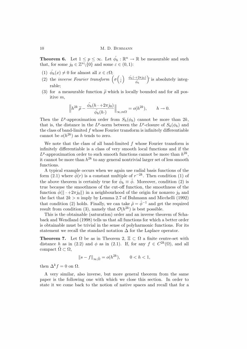
Theorem 6. Let 1 ≤ p ≤ ∞. Let φh : Rn → R be measurable and such

that, for some j0 ∈ Zn\0 and some ε ∈ (0, 1):

(1) φh(x) 6= 0 for almost all x ∈ εΩ;

(2) the inverse Fourier transform(σ(·ε

)φh(·+2πj0)

φh

)is absolutely integ-

rable;

(3) for a measurable function ρ which is locally bounded and for all pos-itive m, ∥∥∥h2k ρ− φh(h ·+2πj0)

φh(h·)∥∥∥∞,mΩ

= o(h2k), h→ 0.

Then the Lp-approximation order from Sh(φh) cannot be more than 2k,that is, the distance in the Lp-norm between the Lp-closure of Sh(φh) andthe class of band-limited f whose Fourier transform is infinitely differentiablecannot be o(h2k) as h tends to zero.

We note that the class of all band-limited f whose Fourier transform isinfinitely differentiable is a class of very smooth local functions and if theLp-approximation order to such smooth functions cannot be more than h2k,it cannot be more than h2k to any general nontrivial larger set of less smoothfunctions.

A typical example occurs when we again use radial basis functions of theform (2.1) where φ(r) is a constant multiple of r−2k. Then condition (1) of

the above theorem is certainly true for φh ≡ φ. Moreover, condition (2) istrue because the smoothness of the cut-off function, the smoothness of thefunction φ(‖ · +2πj0‖) in a neighbourhood of the origin for nonzero j0 andthe fact that 2k > n imply by Lemma 2.7 of Buhmann and Micchelli (1992)

that condition (2) holds. Finally, we can take ρ = φ−1 and get the requiredresult from condition (3), namely that O(h2k) is best possible.

This is the obtainable (saturation) order and an inverse theorem of Scha-back and Wendland (1998) tells us that all functions for which a better orderis obtainable must be trivial in the sense of polyharmonic functions. For itsstatement we recall the standard notation ∆ for the Laplace operator.

Theorem 7. Let Ω be as in Theorem 2, Ξ ⊂ Ω a finite centre-set withdistance h as in (2.2) and φ as in (2.1). If, for any f ∈ C2k(Ω), and allcompact Ω ⊂ Ω,

‖s− f‖∞,Ω = o(h2k), 0 < h < 1,

then ∆kf = 0 on Ω.

A very similar, also inverse, but more general theorem from the samepaper is the following one with which we close this section. In order tostate it we come back to the notion of native spaces and recall that for a


radial basis function with positive distributional Fourier transform φ(‖ · ‖) :Rn \ 0 → R, the square of the native space norm is

‖f‖2φ :=

1

(2π)n

∫1

φ(‖t‖) |f(t)|2 dt (2.5)

and the native space X is the space of all distributions f on Rn for which

(2.5) is finite. In the case of the thin-plate splines or, more generally, (2.1),

X agrees with D−kL2(Rn), because φ(‖t‖)−1 is a constant multiple of ‖t‖2k,and by the Parseval–Plancherel theorem (Stein and Weiss 1971); this being

a special case, other positive φ are admitted as well. For the statement ofthe following theorem we recall that the radial basis function is conditionallypositive definite of order k in R

n if the matrix A with centres from Ξ ⊂ Rn

is nonnegative definite on the subspace of coefficient vectors λ ∈ RΞ that

are orthogonal to Pk−1n (Ξ). The functions (2.1) are all conditionally positive

definite of order k subject to a possibly needed sign change. We use thenotation τ(x) ∼ t(x) if both τ(x)/t(x) and t(x)/τ(x) are uniformly boundedfor the appropriate range of x.

Theorem 8. Let Ω be a bounded domain containing a Pk−1n -unisolvent

subset. Let φ be conditionally positive definite of order k and satisfy

φ(r) ∼ r−2k, r > 0.

If f ∈ C(Ω) and there exists µ > k such that

‖s− f‖∞,Ω ≤ Chµ, h→ 0,

for the radial basis function interpolants s defined on all finite sets of centresΞ ⊂ Ω with h given by (2.2), then f is an element of X. (The constant Cdepends on f but not on h.)

An example for the application of this result is the radial basis function(2.1) with k there and in Theorem 8 being the same.

3. Compact support

This section deals with radial basis functions that are compactly supported,quite in contrast to everything else we have seen before in this article. All ofthe radial basis functions that we have considered so far have global support,and in fact many of them, such as multiquadrics, do not even have isolatedzeros (thin-plate splines do, by contrast). Moreover, the radial basis func-tions φ(r) are usually increasing with growing argument r → ∞, so thatsquare-integrability, for example, and especially absolute integrability areimmediately ruled out. In most cases, this poses no severe restrictions; wecan, in particular, interpolate with these functions and get good convergencerates nonetheless, as we have seen in the previous section. There are, how-ever, practical applications that demand local support of the basis functions

12 M. D. Buhmann

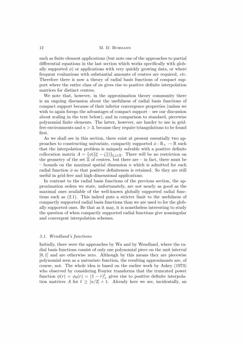
such as finite element applications (but note one of the approaches to partialdifferential equations in the last section which works specifically with glob-ally supported φ) or applications with very quickly growing data, or wherefrequent evaluations with substantial amounts of centres are required, etc.Therefore there is now a theory of radial basis functions of compact sup-port where the entire class of φs gives rise to positive definite interpolationmatrices for distinct centres.

We note that, however, in the approximation theory community thereis an ongoing discussion about the usefulness of radial basis functions ofcompact support because of their inferior convergence properties (unless wewish to again forego the advantages of compact support – see our discussionabout scaling in the text below), and in comparison to standard, piecewisepolynomial finite elements. The latter, however, are harder to use in grid-free environments and n > 3, because they require triangulations to be foundfirst.

As we shall see in this section, there exist at present essentially two ap-proaches to constructing univariate, compactly supported φ : R+ → R suchthat the interpolation problem is uniquely solvable with a positive definitecollocation matrix A = φ(‖ξ − ζ‖)ξ,ζ∈Ξ. There will be no restriction onthe geometry of the set Ξ of centres, but there are – in fact, there must be– bounds on the maximal spatial dimension n which is admitted for eachradial function φ so that positive definiteness is retained. So they are stilluseful in grid-free and high-dimensional applications.

In contrast to the radial basis functions of the previous section, the ap-proximation orders we state, unfortunately, are not nearly as good as themaximal ones available of the well-known globally supported radial func-tions such as (2.1). This indeed puts a stricter limit to the usefulness ofcompactly supported radial basis functions than we are used to for the glob-ally supported ones. Be that as it may, it is nonetheless interesting to studythe question of when compactly supported radial functions give nonsingularand convergent interpolation schemes.

3.1. Wendland’s functions

Initially, there were the approaches by Wu and by Wendland, where the ra-dial basis functions consist of only one polynomial piece on the unit interval[0, 1] and are otherwise zero. Although by this means they are piecewisepolynomial seen as a univariate function, the resulting approximants are, ofcourse, not. The whole idea is based on the earlier work by Askey (1973)who observed by considering Fourier transforms that the truncated powerfunction φ(r) = φ0(r) = (1 − r)`+ gives rise to positive definite interpola-tion matrices A for ` ≥ [n/2] + 1. Already here we see, incidentally, an


upper bound on the spatial dimension n if we fix the degree of the piecewisepolynomial.

In order to derive a large class of compactly supported radial basis func-tions starting from Askey’s result, Schaback and Wu (1995) introduced thetwo so-called operators on radial functions

Df(x) := −1

xf ′(x), x > 0,

and

If(x) :=

∫ ∞

xrf(r) dr, x > 0,

that are defined for suitably differentiable or asymptotically decaying f , re-spectively, and are inverse to each other. Additive polynomial terms donot arise on integration since we always restrict ourselves to compactly sup-ported functions. Next, Wendland (1995) and Wu (1995) use the fact thatthe said interpolation matrix A for the truncated power φ0 remains positivedefinite if the basis function

φ(r) = φn,k(r) = Ikφ0(r), r ≥ 0, (3.1)

is used when ` = k+[n/2]+1. The way to establish that fact is by consideringthe Fourier transform of the n-variate radially symmetric function φ(‖ · ‖),which is also radially symmetric and computed by the univariate Hankeltransform

φ(r) = (2π)n/2r1−n/2∫ ∞

0sn/2Jn/2−1(rs)φ(s) ds, r = ‖x‖ ≥ 0, (3.2)

where Jn/2−1 is a Bessel function. This is the radial part of the radiallysymmetric Fourier transform of φ(‖ · ‖). Hence we have to show that pos-itivity of the Fourier transform, which is necessary and sufficient for thepositive definiteness of the matrix A by Bochner’s theorem, prevails whenthe operator I above is applied, as long as the restrictions on dimensionare observed. This proof is carried out by studying the action of I on theHankel transform (3.2) and by direct computation and use of identities ofBessel functions.

Starting from this, Wendland (1995, 1998), in particular, developed anentire theory of the radial basis functions of compact support which arepiecewise polynomial and are positive definite. This theory encompassesrecursions for their coefficients when they are expanded in linear combin-ations of powers and truncated powers of lower order, convergence results,and minimality of polynomial degree for given dimension and smoothness.Two results below serve as examples for the whole theory. The first statesthe minimality of degree for given smoothness and dimension and the secondis a convergence result.

14 M. D. Buhmann

Theorem 9. The radial function (3.1) gives rise to a positive definite in-terpolation matrix A with radial basis function φ = φn,k, and with distinctcentres Ξ in R

n. Further, among all such functions for dimension n andsmoothness C2k, it is of minimal polynomial degree.

Theorem 10. Let φ be defined by (3.1), let f be a function in the Sobolevspace Hk+(n+1)/2(Rn), and let k be at least 1 when n = 1 or n = 2. Then,for a compact domain Ω with centres Ξ ⊂ Ω, the interpolant (1.1) satisfies

‖s− f‖∞,Ω = O(hk+1/2

), h→ 0,

where h is given by (2.2).

Examples are, for ` ≥ [n/2] + 1,

φ(r) = (1− r)`+1+ ((`+ 1)r + 1),

φ(r) = (1− r)`+2+ ((`2 + 4`+ 3)r2 + (3`+ 6)r + 3),

in a form proposed by Fasshauer.

3.2. Further contributions

The second class of radial basis functions of compact support (Buhmann1998, 2000) are reminiscent of the famous thin-plate splines, albeit truncatedin a suitable way, and of a certain convolution form. It contains, for instance,the following cases. (We state the value of the function only on the unitinterval; elsewhere it is zero. It can, of course, be scaled suitably dependingon the distances between the centres.)

Namely, two examples that give twice and three-times continuously differ-entiable functions, respectively, in three dimensions and two dimensions areas follows. We state them first because they are useful to illustrate the goalof our later result. The parameter choices for the theorem below α = δ = 1

2 ,ρ = 1, and λ = 2, give, for n = 3,

φ(r) = 2r4 log r − 7

2r4 +

16

3r3 − 2r2 +

1

6, 0 ≤ r ≤ 1,

while the choices α = 34 , δ = 1

2 , ρ = 1, and λ = 2, provide, for n = 2,

φ(r) =112

45r

92 +

16

3r

72 − 7r4 − 14

15r2 +

1

9, 0 ≤ r ≤ 1.

Another two-dimensional (n = 2) example which is twice times continuouslydifferentiable is

φ(r) =1

18− r2 +

4

9r3 +

1

2r4 − 4

3r3 log r, 0 ≤ r ≤ 1.


Theorem 11. Let 0 < δ ≤ 12 , ρ ≥ 1 be reals, and suppose λ 6= 0 and

α > −1 are also real quantities with

λ ∈

(−12 ,∞), α ≤ min[12 , λ− 1

2 ], if n = 1, or

[1,∞), −12 < α ≤ 1

2λ, if n = 1, and

(−12 ,∞), α ≤ min[12(λ− 1

2), λ− 12 ], if n = 2, and

(0,∞), α ≤ 12(λ− 1), if n = 3, and

(12(n− 5),∞), α ≤ 1

2(λ− 12(n− 1)), if n > 3.

Then the radial basis function

φ(r) =

∫ ∞

0

(1− r2/β

)λ+βα(1− βδ)ρ+ dβ, r ≥ 0, (3.3)

has a positive Fourier transform and therefore, by Bochner’s theorem, givesrise to positive definite interpolation matrices A with centres Ξ from R

n.Moreover, φ(‖ · ‖) ∈ C1+d2αe(Rn).

There is also a convergence estimate for the above radial functions avail-able which includes scaling of the radial basis function, because, as thedistances between the centres become smaller, we wish to decrease the sup-port of the radial function as well. Otherwise we would lose the advantagesof compact support since the support relative to the distance between thecentres would increase. Note that, in the statement of the following theorem,the approximand f is continuous by the Sobolev embedding theorem pre-cisely as long as 1 + α is positive by the conditions in the previous theorem(this is therefore a necessary condition).

Theorem 12. Let φ be as in the previous theorem and suppose addition-ally ρ > 1, 2α ≤ λ−n/2−3+bρc. Let Ξ be a finite set in a compact domainΩ. Let s be the scaled interpolant (1.1)

s(x) =∑ξ∈Ξ

λξφ(η−1‖x− ξ‖), x ∈ Rn,

to f ∈ L2(Rn) ∩D−n/2−1−αL2(Rn), with the interpolation conditions s|Ξ =f |Ξ satisfied. Then the uniform convergence estimate

‖f − s‖∞,Ω ≤ Ch1+αη−n/2−1−α

holds for h → 0 and positive bounded η, the positive constant C beingindependent of both h and η.

It is interesting to observe that the function classes of the first subsec-tion of this section can be integrated into the more general class discussedin this subsection. Namely, when the operator D is applied to our radial

16 M. D. Buhmann

functions (3.3), it gives

Dλφ(r) = Γ(λ+ 1)2λ∫ 1

r2βα−λ(1−

√β)ρ dβ, 0 ≤ r ≤ 1,

for δ = 12 and any integral nonnegative λ. Therefore, by one further applic-

ation of the differentiation operator and explicit evaluation,

Dλ+1φ(r) = Γ(λ+ 1)2λ+1r2α−2λ(1− r)ρ+ = Γ(λ+ 1)2λ+1(1− r)ρ+, r ≥ 0,

for α = λ. Now let λ = k− 1, k ≥ 1,ρ = [12n] + k+ 1 and recall that, on theother hand, we know that the radial functions φn,k of Wendland are suchthat

Dkφn,k(r) = (1− r)[ 12n]+k+1

+ , r ≥ 0.

Therefore, the functions generated in this fashion can also be derived from(3.3), albeit with a parameter α that does not fulfil the conditions of The-orem 11, so it is a type of continuation. The functions from Wu (1995) alsobelong to that class as they were shown by Wendland to be special casesof his functions. Therefore, since the class of Wendland functions describedhere contains those introduced by Wu (1995), our class covers both. Finally,because we know that all those functions have positive Fourier transforms,there follow immediately new results about the positivity of Hankel trans-forms (3.2) which extend the work by Misiewicz and Richards (1994), andthis is in spite of the fact that the parameter α here does not yield theconditions of Theorem 11.

4. Iterative methods for implementation

Among the most useful radial basis functions which provide good, accurateapproximations are the thin-plate splines, for instance in two dimensions,and multiquadrics. However, these two, like many other examples of radialbasis functions with global support, lead to linear interpolation systems thatrequire special considerations if |Ξ| is more than a few hundred when wecalculate the coefficients λξ. Otherwise the computational cost of O(|Ξ|3)is prohibitively expensive for direct methods, storage being another majorobstacle if the size of the set of centres is too large – even with the fastestand biggest workstations currently available.

There are several approaches currently under intense investigation, mainlyin Cambridge and in Christchurch, New Zealand, for dealing with this prob-lem, two of which we shall explain here to exemplify what can be done todaywhen we have 50000 centres, say. This is the BGP (Beatson–Goodsell–Powell) method of local Lagrange functions, another highly relevant andsuccessful class of methods being the fast multipole approaches (Beatsonand Newsam (1992); see also Beatson and Light (1997) and Beatson, Cher-rie and Mouat (1999)). Like the fast multipole methods, the BGP algorithm


(Beatson, Goodsell and Powell 1995) is iterative and depends on an initialstructuring of the centres Ξ before the start of the iteration, although thatone is less complicated than the fairly sophisticated hierarchical structuredemanded for the multipole schemes, especially when n > 2.

4.1. The BGP method

We explain the method for n = 2, but we remark that the case n = 3is under investigation and will probably be admissible and have suitablesoftware soon. The special further complication for n = 3 is the importantthree-dimensional structuring of the data; conceptually there are no changesin the algorithm we describe below. We also take thin-plate splines only,although the method has actually been already tested successfully on multi-quadrics as well (Faul and Powell 1999), and once again there are almost nochanges except for a different k which plays an important role below. This isbecause the method makes, as we shall see, extensive use of the variationalproperties explained in Section 2 of this paper, and those can be extendedto multiquadrics, for instance, although they were first found in connectionwith thin-plate splines.

The interpolant we wish to compute still has the same form as in theintroduction for k = n = 2 and φ(r) = r2 log r but we denote the actual,sought interpolant by s∗, whereas s denotes in this section only the activeapproximation to s∗ at each stage of the algorithm. This is useful for de-scribing our iterative scheme. The basic idea of the algorithm is derivedfrom a Lagrange formulation of the interpolant

s∗(x) =∑ξ∈Ξ

f(ξ)Lξ(x), x ∈ Rn, (4.1)

instead of (1.1), where each Lagrange function Lξ satisfies the Lagrangeconditions

Lξ(ζ) = δζξ, ξ, ζ ∈ Ξ, (4.2)

and is of the form

Lξ(x) =∑ζ∈Ξ

λζξφ(‖x− ζ‖) + pξ(x), x ∈ Rn. (4.3)

Here, pξ ∈ P12 and λ·,ξ ⊥ P

12(Ξ) for each ξ as usual. Clearly, the computation

of such full Lagrange functions would be just as expensive as solving thefull usual linear interpolation system of equations. Therefore the idea is toreplace (4.2) by local Lagrange conditions which require for each ξ only thatthe identity holds for some q = 30 points, say, ζ that are nearby ξ. Hencewe take Lagrange functions that are still of the form (4.3) but with at mostq nonzero coefficients. We end up with an approach to our interpolation

18 M. D. Buhmann

problem that resembles a domain decomposition approach, because we di-vide the set of centres into subsets and regard the interpolation method asa local method on those subsets.

So that we can associate with each ξ the Lagrange function Lξ and its‘active’ point set of centres, we call the latter Lξ ⊂ Ξ, |Lξ| = q. In additionto having q elements, Lξ must contain a unisolvent subset with respectto P

k−1n as required before. We also extract another set of centres with a

unisolvent subset Σ of approximately the same size q from Ξ for which nolocal Lagrange functions are computed because that set is sufficiently smallto allow direct solution of the interpolation problem.

In order that an iterative method can be applied, we order the centresΞ \ Σ = ξimi=1 for which local Lagrange functions are computed and havethe final requirement that, for all i = 1, 2, . . . ,m,

ξi ∈ Lξi ⊂ Ξ \ ξ1, ξ2, . . . , ξi−1.We require that the q points in the set above are those among the centresthat follow ξi which are the closest ones to ξi. There may be ties in thenecessary ordering procedure that can be broken randomly. The Lagrangeconditions that must be satisfied by the local Lagrange functions are nowthe locally restricted conditions

Lξ(ζ) = δζξ, ζ ∈ Lξ. (4.4)

We employ the same notation for the local Lagrange functions as for thefull ones, as the latter will no longer occur in this section. Using theselocal Lagrange functions, (4.1) is naturally no longer a representation ofthe exact approximant s∗, but only an approximation thereof, and here iswhere the iteration and iterative correction come in. Of course the Lagrangefunctions, that is, their coefficients, are computed in advance once and forall and stored before the beginning of the iterations. (This is an O(|Ξ|)process.) A useful comparison of this approach with the Newton formulationof univariate polynomial interpolants is made by Powell (1999).

In those iterations, we make an iterative refinement of the approximationat each step of the algorithm by correcting its residual through updates

s(x) −→ s(x) + Lξ(x)× cξ(x),

where

cξ(x) =1

λξξ

∑ζ∈Lξ

λζξ(f(ζ)− s(ζ)). (4.5)

We shall see in the proof of the next theorem why λξξ is positive and wemay therefore divide by λξξ. The correction (4.5) is added for all ξ ∈ Ξ \ Σfor each sweep of the algorithm. The final stage of each sweep consists of


the correction

s(x) −→ s(x) + σ(x),

where σ is the full standard thin-plate spline solution of the interpolationproblem with centres Σ computed with a direct method

σ(ξ) = f(ξ)− s(ξ), ξ ∈ Σ.

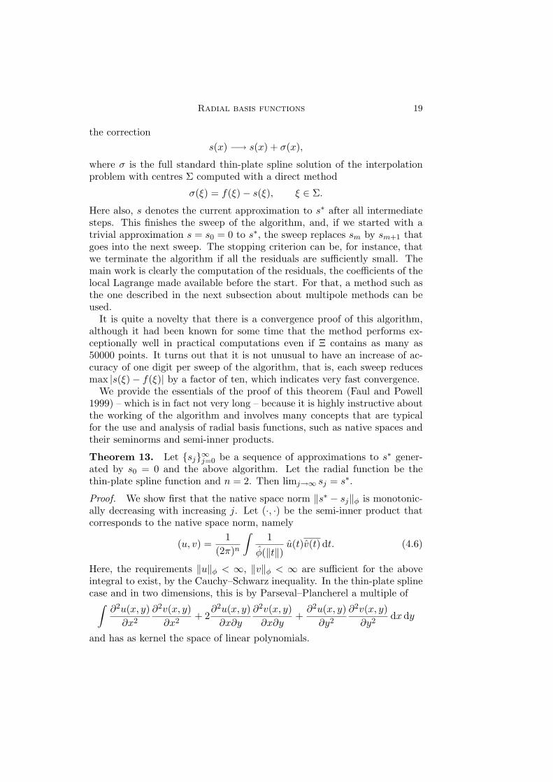
Here also, s denotes the current approximation to s∗ after all intermediatesteps. This finishes the sweep of the algorithm, and, if we started with atrivial approximation s = s0 = 0 to s∗, the sweep replaces sm by sm+1 thatgoes into the next sweep. The stopping criterion can be, for instance, thatwe terminate the algorithm if all the residuals are sufficiently small. Themain work is clearly the computation of the residuals, the coefficients of thelocal Lagrange made available before the start. For that, a method such asthe one described in the next subsection about multipole methods can beused.

It is quite a novelty that there is a convergence proof of this algorithm,although it had been known for some time that the method performs ex-ceptionally well in practical computations even if Ξ contains as many as50000 points. It turns out that it is not unusual to have an increase of ac-curacy of one digit per sweep of the algorithm, that is, each sweep reducesmax |s(ξ)− f(ξ)| by a factor of ten, which indicates very fast convergence.

We provide the essentials of the proof of this theorem (Faul and Powell1999) – which is in fact not very long – because it is highly instructive aboutthe working of the algorithm and involves many concepts that are typicalfor the use and analysis of radial basis functions, such as native spaces andtheir seminorms and semi-inner products.

Theorem 13. Let sj∞j=0 be a sequence of approximations to s∗ gener-ated by s0 = 0 and the above algorithm. Let the radial function be thethin-plate spline function and n = 2. Then limj→∞ sj = s∗.

Proof. We show first that the native space norm ‖s∗ − sj‖φ is monotonic-ally decreasing with increasing j. Let (·, ·) be the semi-inner product thatcorresponds to the native space norm, namely

(u, v) =1

(2π)n

∫1

φ(‖t‖) u(t)v(t) dt. (4.6)

Here, the requirements ‖u‖φ < ∞, ‖v‖φ < ∞ are sufficient for the aboveintegral to exist, by the Cauchy–Schwarz inequality. In the thin-plate splinecase and in two dimensions, this is by Parseval–Plancherel a multiple of∫

∂2u(x, y)

∂x2

∂2v(x, y)

∂x2+ 2

∂2u(x, y)

∂x∂y

∂2v(x, y)

∂x∂y+∂2u(x, y)

∂y2

∂2v(x, y)

∂y2dxdy

and has as kernel the space of linear polynomials.

20 M. D. Buhmann

We start with s = s0 = 0. Each full sweep of the algorithm replaces sjby sj+1, but within each sweep there are further m + 1 updates . By thoseupdates, sj,0 = sj is replaced by sj,1, and so on until sj,m is replaced bysj+1 = sj,m+1 = sj,m + σ where σ is defined above. At the (j − 1)st stage,for each index i, ‖s∗ − sj−1,i−1‖φ is replaced by

‖s∗ − sj−1,i−1 − θξiLξi‖φ,where θξi = cξi . It is elementary that we get

‖s∗ − sj−1,i−1 − θLξi‖2φ = min!

when the linear parameter θ assumes the value

θ =(s∗ − sj−1,i−1, Lξi)

‖Lξi‖2φ

. (4.7)

We claim that (4.7) is the same as θξi and in the proof of this fact we shallalso show as a by-product that the denominator in (4.7) is positive. Indeed,recalling that the additional polynomials used are in the kernel of the innerproduct (4.6), we get from the reproducing kernel identity

‖Lξi‖2φ =

( ∑ζ∈Lξi

λζξiφ(‖ · −ζ‖),∑τ∈Lξi

λτξiφ(‖ · −τ‖))

=∑ζ∈Lξi

λζξi∑τ∈Lξi

λτξiφ(‖ζ − τ‖)

= λξiξi ,

by (4.4) and because pζ is annihilated by the side conditions on the coeffi-cients λζξi . This also shows, incidentally, that the important inequality

λξiξi > 0 (4.8)

holds because ‖Lξi‖2φ is not zero. Otherwise Lξi would be in the kernel of

our semi-inner product and not able to satisfy the cardinality conditions.Moreover, by the same token, we get from the reproducing kernel properties

(s∗ − sj−1,i−1, Lξi) =∑ζ∈Lξi

λζξi(s∗ − sj−1,i−1, φ(‖ · −ζ‖))

=∑ζ∈Lξi

λζξi(s∗(ζ)− sj−1,i−1(ζ))

=∑ζ∈Lξi

λζξi(f(ζ)− sj−1,i−1(ζ)).

Next, we have to consider the alteration to ‖s∗ − sj−1,m‖φ as soon as σ isadded to sj−1,m. In order to prove the monotonic decrease of ‖s∗−sj−1,m‖φ


when this happens, we need to prove that the following inner product van-ishes (

s∗ − sj−1,m − σ,∑τ∈Σ

λτφ(‖ · −τ‖) + p

)

=

(s∗ − sj−1,m − σ,

∑τ∈Σ

λτφ(‖ · −τ‖))

= 0.

In the above, the coefficients λτ are real and p ∈ Pk−1n . This orthogonality

relation is established using the same facts as those we required for showing‖Lξi‖2

φ = λξiξi and therefore we do not repeat the arguments.

In summary, we now know that ‖sj,i − s∗‖φ tends to a limit for all fixedi, and j increasing, because it is bounded below by zero and monotonicallydecreasing, as it is a subsequence of the monotonically decreasing doublyindexed sequence ‖sj,i−s∗‖φ∞j=0,0≤i≤m. Moreover, by the definition of oursemi-inner product

‖s∗ − sj−1,i−1 − θξiLξi‖2φ = ‖sj−1,i−1 − s∗‖2

φ −(s∗ − sj−1,i−1, Lξi)

2

‖Lξi‖2φ

.

Therefore, for all centres

(s∗ − sj−1,i−1, Lξi) → 0, j →∞, ξi ∈ Ξ \ Σ, (4.9)

because ‖sj,i − s∗‖φ converges. In particular, it follows that

(s∗ − sj , Lξ1) → 0, j →∞. (4.10)

Moreover, sj,1 = sj + (s∗ − sj , Lξ1)Lξ1/‖Lξ1‖2φ, so that we also get(

s∗ − sj − (s∗ − sj , Lξ1)Lξ1

‖Lξ1‖2φ

, Lξ2

)→ 0, j →∞.

Therefore

(s∗ − sj , Lξ2) → 0, j →∞,

and indeed

(s∗ − sj , Lξ) → 0, j →∞, ξ ∈ Ξ \ Σ. (4.11)

Finally, we observe

(s∗ − sj , Lξi) =∑ζ∈Lξi

λζξi(s∗(ζ)− sj(ζ)) → 0, j →∞. (4.12)

Recalling that s∗−sj restricted to Σ vanishes anyway, and recalling that λξiξiis positive, we now go backwards and start from i = m with an inductionargument, whereupon (4.8), (4.9) and (4.12) imply sj(ζ) → s∗(ζ) as j →∞

22 M. D. Buhmann

for all ζ ∈ Ξ. This implies sj → s∗ for j → ∞, as demanded, becausethe space spanned by the translates φ(‖ · −ξ‖) plus the polynomial space isfinite-dimensional. 2

4.2. Fast multipole methods

Another approach for approximation and iterative refinement to the ra-dial basis function interpolants is that of fast multipole methods. Thesealgorithms are based on analytic expansions of the underlying radial func-tions for large argument. We see that this is possible for all non-compactlysupported radial basis functions that have been mentioned, because they aresmooth away from their centres. For the compactly supported ones, the ap-proach for fast evaluation and solution of the linear system is, of course, notrequired. The salient ideas date back to a paper of Greengard and Rokhlin(1987) where the methods are used to solve numerically integral equations –this is related to our radial basis function approximations because the sumsand coefficients (‘weights’) can be viewed as discretizations of integrals.

The methods require structuring the data in a hierarchical way before theonset of the iteration, and computing so-called far-field expansions (Laurentseries expansions for large arguments, as already alluded to) in advance.The goal is to reduce the cost of a single approximate evaluation of theradial function sum down to O(1) and storage to O(|Ξ|). The far-fieldexpansions exploit the fact that radial basis functions of the form (2.1)are analytic except at the origin, even when made multivariate throughcomposition with Euclidean norms. Therefore, they can be approximatedwell away from the origin by a truncated Laurent expansion. The accuracy(that is, the length of the truncated expansion) to this can be preset andmade to match any chosen accuracy ε, for instance a small positive multipleof the machine precision of the computer in use, but of course the cost ofthe method, that is, the multiplier in the operation count, rises with largeraccuracy. In tandem with the hierarchical structure of the centre-set, whichwe shall explain in some detail below, this allows approximative evaluationof many radial basis function terms whose centres are close to each othersimultaneously by a single finite Laurent expansion that is inexpensive, aslong as the argument x is far from the said cloud of centres. By contrast, allradial functions whose translates are close to x are computed exactly andexplicitly. We shall call those centres the near field below.

The hierarchical structure of the centres is fundamental to the algorithmbecause it decides and orders what is far and what is near any given xwhere we wish to evaluate. It is built up as follows. We assume for the sakeof an easy exposition that Ξ ⊂ [0, 1]2 and that the ξ are fairly uniformlydistributed in that unit square so that uniform subdivisions are acceptable.We form a quad-tree of centres which contains as a root Ξ and as the next


children the intersections of the four quarter squares of the unit square withΞ. They are in turn divided into four grandchildren each in the same fashion.We stop this process at a predetermined level that in part determines theaccuracy of the calculation in the end. Each member of this family is calleda panel. We point out that there are implementations where the divisionsare only by two and not by four (Powell 1993). There is no principal reasonfor making this choice that forms a binary tree instead of a quad-tree andboth approaches have been tried successfully.

Now we must define the far field and the near field for each x where s(x) iscomputed. Given x, all centres ξ that are in the near field give rise to explicitevaluations of φ(‖x − ξ‖). The near field consists simply of contributionsfrom all points which are not ‘far’, according to the following definition: wesay x is far away from a panel T and therefore from all centres in that panel,if there is at least one more panel between x and T , and if this panel is onthe same level of parenthood as T itself.

Next, we have to decide how to group the far points. All panels Q arein the evaluation list of a panel T if Q is either at the same or a coarser(higher) level than T and every point in T is far away from Q, and if, finally,T contains a point that is not far away from the parent of Q. Thus the farfield of an x whose closest centre is in a panel T is the sum of all

sQ(x) =∑ξ∈Q

λξφ(‖x− ξ‖) (4.13)

such that Q is in the evaluation list of T . For each (4.13), a common Laurentseries is computed. Since we do not know the value of x that is to be insertedinto (4.13), we compute the coefficients of the Laurent series and insert xlater on.

In a set-up process, we compute these expansions of the radial function forlarge argument, that is, their coefficients, and store them; when x is providedat the evaluation stage, we combine those expansions for all centres fromeach evaluation list, and in an additional, final step we can simplify furtherby approximating the whole far field by one Taylor series.

A typical Laurent series expansion to thin-plate spline terms, which westill use as a paradigm for algorithms with more general classes of radial basisfunctions, is as follows. To this end, we work in two dimensions n = 2 andidentify two-dimensional real space with one-dimensional complex space.

Lemma 1. Let z and t be complex numbers, and let

φt(z) := ‖t− z‖2 log ‖t− z‖.Then, for all ‖z‖ > ‖t‖, and denoting the real part by Re ,

φt(z) = Re

(z − t)(z − t)

(log z −

∞∑k=1

1

k

(t

z

)k)

,

24 M. D. Buhmann

which is the same as

(‖z‖2 − 2Re (tz) + ‖t‖2) log ‖z‖+ Re

∞∑k=0

(akz + bk)z−k,

where bk = −tak and a0 = −t and ak = tk+1/[k(k + 1)] for positive k.Moreover, if the above series is truncated after p + 1 terms, the remainderis bounded above by

‖t‖2

(p+ 1)(p+ 2)

c+ 1

c− 1

(1

c

)p

with c = ‖z/t‖.In summary, the principal steps of the whole algorithm are as follows.

Set-up

(1) Perform the repeated subdivision of the square down to log |Ξ| levelsand sort the elements of Ξ into the finest level panels.

(2) Form the Laurent series expansions (i.e., compute their coefficients) forall fine level panels R.

(3) Translate centres of expansions so that the expansions can be re-usedfor other centres and, by working up the tree towards coarser levels,form analogous expansions for all less refined levels.

(4) Working down the tree from the coarsest level, compute Taylor expan-sions of the whole far field for each panel Q.

Evaluation at x

(1) Locate the finest level panel Q containing the centre closest to x.(2) Evaluate s(x) by computing near field contributions explicitly and by

using the Taylor approximation of the entire far field. For the far field,we use all panels that are far away from x and are not subsets of anycoarser panels already considered.

The computational cost without set-up is O(|Ξ|) because of the hierarchicalstructure. The set-up cost isO(log |Ξ|), because of the tree structure, but theconstant contained in this estimate may be large because of the computationof the various expansions and the design of the tree. This is so although eachexpansion is an O(1) procedure. In practice it turns out that the method issuperior to direct computation if |Ξ| is at least of the order of 200 points.

In which way is this algorithm now related to the computation of inter-polation coefficients? It is related in one way because the efficient evaluationof the linear combination of thin-plate spline translates is required in thefirst algorithm presented in this section. There the residuals fξ−s(ξ) playedan important role, s(ξ) being the current linear combination of thin-plate


splines at a centre and the current approximation to the solution we re-quire. Therefore, to make the BGP algorithm efficient, fast evaluation of sis needed, partly because our radial basis functions are conditionally posit-ive definite (the preconditioning making the matrices positive (semi-)definitematrices) and partly because the condition numbers severely influence theconvergence properties of conjugate gradient methods.

However, the importance of fast availability of residuals is not only re-stricted to the BGP method. Other iterative methods for computing radialbasis function interpolants such as conjugate gradient methods are also inneed of these residuals. In order to apply those, however, a preconditioningmethod is usually needed.

There are various possible improvements to the algorithm of this subsec-tion. For instance, we can use an adaptive method for subdividing into thehierarchical structure of panels, so that the panels may be of different sizes,but always contain about the same number of centres. This is particularlyadvantageous when the data are highly non-uniformly distributed.

5. Interpolation on spheres

Because of the many applications that suit radial basis functions in geodesy,there is already a host of papers that specialize radial basis function approx-imation and interpolation to spheres. Freeden and co-workers (1981, 1986,1995) have made a very large number of contributions to this aspect of ap-proximation theory of radial basis functions. There are excellent and longreview papers available from the work of this group (see the cited references)and we will therefore be relatively brief in this section. Of course, we nolonger use the conventional Euclidean norm in connection with a univariateradial function when we approximate on the (n − 1) sphere Sn−1 withinRn but apply so-called geodesic distances. Therefore the standard notions

of positive definite functions and conditional positive definiteness no longerapply, and one has to study new concepts of (conditionally) positive defin-ite functions on the (n − 1) sphere. This started with Schoenberg (1942),who characterized positive definite functions on spheres as those ones whoseexpansions in series of Gegenbauer polynomials always have nonnegativecoefficients. Xu and Cheney (1992) studied strict positive definiteness onspheres and gave necessary and sufficient conditions. This was further gen-eralized by Ron and Sun in 1996

Recent papers by Jetter, Stockler and Ward (1999) and Levesley, Light,Ragozin and Sun (1999) use native spaces, (semi-)inner products and repro-ducing kernels (cf. Saitoh (1988) for a treatise on the theory of reproducingkernels) to derive approximation orders in a very similar fashion to the work

summarized in Section 2. They all apply the spherical harmonics Y (`)k d`k=1

that form an orthonormal basis of the d`-dimensional space of polynomials

26 M. D. Buhmann

on the sphere in P`n(S

n−1) ∩ P`−1n (Sn−1)⊥. They are called spherical har-

monics because they are the restrictions of polynomials of total degree ` tothe sphere and are in the kernel of the Laplace operator ∆. The dimensiond` is computable, and this is not difficult, but it is not important to us atthis stage.

Then, a native space X is defined for all expansions of functions on thesphere in spherical harmonics: namely, the native space’s elements are

f(x) =

∞∑`=0

d∑k=1

f`kY(`)k (x), x ∈ Sn−1, (5.1)

whose coefficients f`k satisfy certain square summability conditions withprescribed positive real weights a`k. In other words, the native space isdefined by

X =

f∣∣∣ ∞∑`=0

d∑k=1

|f`k|2a`k

<∞. (5.2)

The native space X given in (5.2) and functions (5.1) will give rise to areproducing kernel that is positive definite, but if we enlarge the space bystarting the first sum in (5.2) only at ` = κ and thereby weakening condi-tions, we can also get conditionally positive definite (reproducing) kernels(Levesley et al. 1999) for the ensuing spaces Xκ. Then the native space willbe a semi-Hilbert space, that is, the inner product that we shall describeshortly has a nullspace

K =

f∣∣∣f =

κ−1∑`=0

d∑k=1

f`kY(`)k

.

Now, a standard choice for the positive weights for defining the space Xwhich are often independent of k is a`k = (1 + λ`)

−s. This gives rise to theSobolev space Hs(Sn−1). Here the λ` = `(` + n− 2) are eigenvalues of theLaplace–Beltrami operator.

The inner product that the native space is equipped with can be describedby

〈f, g〉 =

∞∑`=0

d∑k=1

1

a`kf`kg`k,

where the coefficients are defined through (5.1); they are still assumed tobe positive. The reproducing kernel that results from this Hilbert space Xwith the above inner product and that corresponds to the function of ourprevious radial basis functions in the native space is, when x and y are on


the sphere,

φ(x, y) =

∞∑`=0

d∑k=1

a`kY(`)k (x)Y

(`)k (y), x, y ∈ Sn−1. (5.3)

This can be simplified by the famous addition theorem (Stein and Weiss1971) to φ(x, y) = φ(xT y), where

φ(t) =1

ωn−1

∞∑`=0

d`a`kP`(t), (5.4)

ωn−1 being the measure of the unit sphere, if the coefficients are constantwith respect to k. Here, the d` are as above and P` is a Gegenbauer poly-nomial (Abramowitz and Stegun 1972) normalized by P`(1) = 1. Therefore,we now use (5.3) or (5.4) for interpolation on the sphere, in the same placeand with the same centres Ξ as before, but they are from the sphere them-selves of course. Convergence estimates are available from all three sourcesmentioned above that vary in approaching the convergence question. Usingthe mesh norm

h = supx∈Sn−1

infξ∈Ξ

arccos(xT ξ),

Jetter et al. prove the following theorem. The notation |Ξ| is for the cardin-ality of the set Ξ as before.

Theorem 14. Let X and Ξ be as above with the given mesh norm h. Letκ be a positive integer such that h ≤ 1/(2κ). Then, for any f ∈ X, there isa unique interpolant s in

span φ(ξ, ·) | ξ ∈ Ξthat interpolates f on Ξ and satisfies the error estimate

‖s− f‖2∞ ≤ 5(|Ξ|+ 1)

ωn−1‖f‖2

φ

∞∑`=κ+1

(d` max

k=1,...,d`a`k

). (5.5)

Corollary 1. Let the assumptions of the previous theorem hold and sup-pose further that |Ξ|+ 1 ≤ C1κ

n−1 and

C2

1 + κ≤ h ≤ 1

2κ.

Then the said interpolant s provides

‖s− f‖∞ = O((

h

C2

)(α−n)/2)

or

‖s− f‖∞ = O(

exp(−αC2/2h)

h(n−1)/2

),

28 M. D. Buhmann

respectively, if d`×maxd`k=1 a`k is bounded by a constant multiple of (1+`)−αfor an α > n or by a constant multiple of exp(−α(1 + `)) for a positive α,respectively.

An error estimate of Levesley et al., which includes conditionally positivedefinite kernels for κ = 1 or κ = 2, is as follows, for n = 2 (see also Freedenand Hermann (1986) for a similar, albeit slightly weaker result).

Theorem 15. Let X, Ξ, h and κ be as above, let s be the minimal norminterpolants to f ∈ Xκ on Ξ. When φ is twice continuously differentiableon [1− ε, ε] for some ε ∈ (0, 1), then

‖s− f‖∞ ≤ Ch2‖f‖φ,so that, in particular, a polynomial p ∈ P

κ−13 (S2) is added to the s used in

Theorem 14.

6. Applications

6.1. Numerical solution of partial differential equations

Given that radial basis functions are known to be useful to approximatemultivariate functions efficiently, it is suitable to apply them to approxim-ate solutions of partial differential equations numerically. Three approacheshave been tried and tested in this direction, namely collocation techniques,variational formulations and boundary element methods, all in order to solveelliptic partial differential equations with boundary values given. There arevarious reasons why radial basis functions are useful for these three ap-proaches. The first of these is useful because we know much about existenceand accuracy of radial basis function interpolants, especially when the dataare scattered, which is useful for non-grid collocation. The second resemblestypical finite element applications, where usually radial basis functions ofcompact support are used to mimic the standard finite element approachwith multivariate piecewise polynomials. Finally, boundary element meth-ods are suitable in several cases when radial basis functions are known tobe fundamental solutions (Green’s functions) of elliptic partial differentialoperators, most notably powers of the Laplace operator. An example is thethin-plate spline radial basis function and the bi-Laplacian operator. Afterall, in boundary element methods, explicit solutions of the associated homo-geneous problem are required in advance, for which it is immensely helpfulto have Green’s functions to work with.

Naturally, an important decision is the choice of radial basis function,especially whether globally or locally supported ones should be used. Ina Galerkin approach, locally supported elements are almost always em-ployed. Further, the use of radial basis functions becomes particularly in-teresting when nonlinear partial differential equations are solved or non-grid


approaches are used, for instance because of non-smooth domain boundar-ies, where non-uniform knot placement is always important to modelling thesolution to good accuracy.

We begin with a description of the collocation approach, which is thefirst approach one is tempted to try because of our knowledge of interpol-ation properties of the radial basis functions. The first important decisionis whether to use the well-known, standard globally supported radial func-tions such as multiquadrics or the new compactly supported ones that aredescribed earlier in this review. Since the approximation properties of thelatter are not as good as the former ones, we have a trade-off between ac-curacy on one hand and sparsity of the collocation matrix on the otherhand. Compactly supported ones, if scaled suitably, give banded colloca-tion matrices, while the globally supported ones give no sparsity to speakof. When we use the compactly supported radial functions we have, in fact,another trade-off which we have not mentioned so far, because even theirscaling pits accuracy against sparseness of the matrix. If we impose no scal-ing to the radial basis function as in Theorem 12, we do have satisfactoryconvergence, as shown in Theorem 10, but basically the radial basis functionbehaves as a globally supported one, with essentially full matrices, since thecentres become dense in each of the radial functions’ supports. In the otherextreme case, when we scale so that there is always a uniformly boundednumber of centres inside each support, we run the risk of losing convergencealtogether – but the interpolation matrix may be diagonal (and nonsingular,of course). There are several approaches to fixing this problem, and we willmention two of them while describing algorithms.

One typical linear partial differential equation problem suitable for col-location techniques reads

Lu(x) = f(x), x ∈ Ω ⊂ Rn, (6.1)

Bu|∂Ω = q, (6.2)

where Ω is a domain with suitably smooth – at least Lipschitz-continuous –boundary ∂Ω and f , q are prescribed functions. Here L is a linear differentialoperator and B a boundary operator. We will soon come to some specificnonlinear examples in the context of boundary element techniques.

The usual approach to collocation is then for centres Ξ that are partitionedin two disjoint sets Ξ1 and Ξ2, the former from the domain, the latter fromits boundary, to solve the Hermite–Birkhoff interpolation system

ΛξuΞ = f(ξ), ξ ∈ Ξ1,ΛζuΞ = q(ζ), ζ ∈ Ξ2. (6.3)

30 M. D. Buhmann

The approximants uΞ are defined by the sums

uΞ(x) =∑ξ∈Ξ1

cξΛξφ(‖x− ξ‖) +∑ζ∈Ξ2

dζΛζφ(‖x− ζ‖).

The Λξ and Λζ are suitable discrete functionals to describe our operators Land B on the discrete set of centres. In the above display the operators areapplied with respect to the variable x. Examples for such discrete function-als to replace the operators L and B are obtained, for example, by replacingderivatives by symmetric differences or one-sided differences for the bound-ary in case of Neumann problems. Thus we end up with a square symmetricsystem of linear equations whose collocation matrix is nonsingular if, forinstance, the radial basis function is positive definite, smooth enough forapplication of the operators Λ, and the discrete linear functionals are lin-early independent functionals in the dual space of the native space of theradial basis functions (see Section 2 and Wu (1992) for the details). An errorestimate is given in Franke and Schaback (1998). For those error estimates,it has been noted that more smoothness of the radial basis function is re-quired than for a comparable finite element setting in order to get the sameapproximation orders, but clearly, the radial basis function setting has thedistinct advantage of availability in any dimension and the absence of gridsor triangulations.

If a compactly supported radial basis function is used, the necessary scal-ing leads to the aforementioned trade-off between accuracy and bandwidthof the matrix. In fact, the conditioning of the collocation matrix is also af-fected, becoming worse with smaller η, with φ(·/η) being used, although thematrix is positive definite. A Jacobi preconditioning by the diagonal valueshelps here, so the matrix A is replaced by P−1AP−1 where P =

√diag(A),

the diagonal elements of the matrix being positive. Moreover, one canuse a multilevel method (Narcowich, Schaback and Ward (1999), Fasshauer(1999)) where numerical approximations ukNk=0 are computed on nestedsets of centres Ξk ⊃ Ξk−1, k = 1, 2, . . . , N , ΞN = Ξ, and, within each sweepof the algorithm, a new approximation to the desired solution is computedas follows. For instance, to solve Lu = f on the domain Ω with Dirich-let boundary conditions only, at each step k of one sweep one computes,starting with u0 = 0,

Luk = (f − Luk−1)

and sets uk = uk + uk−1. Unfortunately, little is known about the conver-gence behaviour of such a multilevel method.

In the event that a Galerkin method is applied, for instance, to the Helm-holtz equation with Neumann conditions when L = −∆ + I and B = ∂

∂n ,we end up with a square system of linear equations, the stiffness equationsfor uΞ,

a(uΞ, φ(‖ · −ξ‖)) = (f, φ(‖ · −ξ‖))L2(Ω), ξ ∈ Ξ,


with

a(u, v) =

∫Ω(∇u)T (∇v) + uv.

If φ is a radial basis function of compact support such that its Fouriertransform satisfies the decay estimate |φ(r)| = O(r−2k), then Franke andSchaback (1998) establish the convergence estimate

‖u− uΞ‖H1(Ω) ≤ Chσ−1‖u‖Hσ(Ω),

where h is given by (2.2) and k ≥ σ > n/2 + 1.We now outline the third method, that is, a boundary element (BEM)

method, following Pollandt (1997). The dual reciprocity method uses thesecond Green’s formula and a fundamental solution φ(‖ · ‖) of the Laplaceoperator ∆, in order to reformulate a boundary value problem as a boundaryintegral problem over a space of one dimension lower. This will then leadthrough discretization to a linear system with a full matrix for collocation byradial basis functions, in the way familiar from other applications of radialbasis function interpolation. The radial basis function that occurs in thatcontext is this fundamental solution, and, naturally, it is highly relevant inthis case that the Laplace operator is rotationally invariant and has radialfunctions as Green’s functions. We give a concrete example. Namely, for anonlinear problem on a domain Ω ⊂ R

n with Dirichlet boundary conditionssuch as the following one with a nonlinear right-hand side

∆u(x) = u2(x), x ∈ Ω ⊂ Rn, (6.4)

u|∂Ω = q, (6.5)

the goal is to approximate the solution u of the elliptic partial differentialequation on the domain by g plus a boundary term r that satisfies ∆r ≡ 0on the domain. To this end, one gets after an application of Green’s formulathe equation on the boundary that u(x) is the same as∫

Ωu(y)2φ(‖x− y‖) dy −

∫∂Ω

φ(‖x− y‖) ∂

∂nyu(y)− u(y)

∂

∂nyφ(‖x− y‖) dΓy

(6.6)for x ∈ Ω, where ∂

∂nyis the normal derivative with respect to y on Γ = ∂Ω.

The radially symmetric φ is still the fundamental solution of the Laplaceoperator used in the formulation of the differential equation above. Further,one gets after two applications of Green’s formula the equation

1

2(u(x)− g(x)) +

∫∂Ω

φ(‖x− y‖)× ∂

∂ny(u(y)− g(y)) −

(q(y)− g(y))∂

∂nyφ(‖x− y‖) dΓy = 0, x ∈ ∂Ω.

We will later use this equation to approximate the boundary part of the

32 M. D. Buhmann

solution, that is, the part satisfying the boundary conditions. Now we as-sume that there are real coefficients λξ such that the infinite expansion(which will be truncated later on)

u2(y) =∑ξ

λξ φ (‖y − ξ‖), y ∈ Ω,

holds, and set

g(y) =∑ξ

λξ Φ (‖y − ξ‖), y ∈ Ω,

so that ∆g = u2 everywhere with no boundary conditions. Therefore weare first solving a homogeneous problem. Here φ is a suitable radial basisfunction, which is to be distinguished from the fundamental solution φ,with ∆Φ (‖ · ‖) = φ(‖ · ‖), and the centres ξ are from Ω. We now replace theinfinite sums by finite ones (i.e., we approximate the infinite expansions byfinite sums for a suitable Ξ), so that exchanging summation and the Laplaceoperator and term-by-term differentiation in the sum is admitted:

u2(y) =∑ξ∈Ξ

λξ φ (‖y − ξ‖), y ∈ Ω, (6.7)

and

g(y) =∑ξ∈Ξ

λξ Φ (‖y − ξ‖), y ∈ Ω.

We require that the equation in the display after (6.6) holds for finitely manypoints x = ζj ∈ ∂Ω, j = 1, 2, . . . , t, only. Then we solve for the coefficientsλξ by requiring that (6.7) holds for y = ξ, for all ξ ∈ Ξ. This fixes the λξ byinterpolation (collocation in the language of differential equations), whereasthe equation after (6.6) determines the normal derivative ∂

∂nyu(y) on ∂Ω,

where we are replacing ∂∂ny

u(y) by another approximant, a polynomial

spline τ(y), for instance. Thus the spline is found by requiring the aboveequation for all x = ζj ∈ ∂Ω, j = 1, 2, . . . , t, and choosing a suitable t.Finally, an approximation u(x) to u(x) is determined on Ω by the identity

u(x) := g(x) +

∫∂Ω

(q(y)− g(y))∂

∂nyφ(‖x− y‖) dΓy−∫

∂Ωφ(‖x− y‖)

(τ(y)− ∂g(y)

∂ny

)dΓy, x ∈ Ω, (6.8)

where the boundary term r corresponds to the second term on the right-handside of the display.

Now, all expressions on the right-hand side are known. This is an outlineof the approach but we have skipped several important details. Nonethe-less, one can clearly see how radial basis functions appear in this algorithm;


indeed, it is most natural to use them here, since many of them are funda-mental solutions of Laplace operators or their iterates in certain dimensions.In the above example and n = 2, φ(r) = (2π)−1 log r, φ(r) = r2 log r (thin-

plate splines) and Φ(r) = 116 r4 log r − 1

32 r4 are the correct choices. Asthe collocation matrices that appear in the boundary integral equation weare left with in the method are dense and as interpolation is not absolutelynecessary in this approach, it can be substituted by quasi-interpolation.Quasi-interpolation has asymptotically essentially the same approximationbehaviour (i.e., convergence speed) as interpolation but does not requireany data-dependent linear systems to be solved; see also Buhmann (1990a).Convergence theorems for the method are available in the paper by Pollandt.

6.2. Other applications

We outline a few further practical applications of radial basis functions.They include, for example, mappings of two- or three-dimensional imagessuch as portraits or underwater sonar scans into other images for comparison.Here interpolation comes into play because some special features of an imagemay have to be preserved while others need not be mapped exactly, thusenabling a comparison of some features that may differ while at the sametime retaining others. Such so-called ‘markers’ can be, for example, certainpoints of the skeleton in an x-ray that has to be compared to another one,taken at another time. The same structure appears if we wish to comparesonar scans of a harbour at different times, the rocks being suitable asmarkers this time. Thin-plate splines turned out to be excellent for suchvery practical applications (Barrodale and Zala 1997, 1999). Work of thiskind led to the invention of the methods for fast evaluation of thin-platesplines and other radial basis functions discussed above, because, after theinterpolation, the computed interpolant had to be evaluated on a very finesquare grid in two dimensions for analysis or display (Powell 1993).

Measurements of gravitational potential or temperature on the Earth’ssurface at ‘scattered’ meteorological stations or measurements on other mul-tidimensional objects, may give rise to interpolation problems that requirescattered data. Multiquadric approximations are performing well for thistype of use (Hardy 1990). Much work on radial basis functions on sphereswhich we have only touched upon in this article originates from those ap-plications of geophysics.

Many applications involve high-dimensional interpolation or approxima-tion problems when data are coming through many ‘channels’, for instanceelectrodes measuring brain activity from nerve cells. Typical applicationsfrom neural physics produce 50–100 dimensional data taken from those elec-trodes recording measurements from the brain and require post-processingfor smoothing, for example. Radial basis functions have been used extens-

34 M. D. Buhmann

ively for this (e.g., Eckhorn (1999), Hochreiter and Schmidhuber (1999),Anderson, Das and Keller (1998)).

The approximation to so-called learning situations by neural networksusually leads to very high-dimensional interpolation problems with scattereddata. Girosi (1992) mentions radial basis functions as a very suitable ap-proach to this, partly because of their availability in arbitrary dimensions,and their smoothness. A typical application is in fire detectors. An advancedtype of fire detector has to consider several measured parameters, such ascolour, spectrum, intensity, movement of an observed object from which itmust decide whether, for instance, it is looking at a fire in the room or not,because the apparent fire is reflected sunlight. There is a learning procedurebefore the implementation of the device, where several prescribed situations(these are the data) are tested and the values zero (no fire) and one (fire)are interpolated, so that the device can ‘learn’ to interpolate between thesestandard situations for general cases later when it is used in real life. Radialbasis function methods have been tried very successfully for this applicationbecause they are excellent tools for high-dimensional problems that willundoubtedly find many more applications in real life, such as polynomialsplines have done in at least the last 30 years and still do now.

REFERENCES

M. Abramowitz and I. Stegun, eds (1972), Handbook of Mathematical Functions,National Bureau of Standards, Washington.

R. W. Anderson, S. Das and E. L. Keller (1998), ‘Estimation of spatiotemporalneural activity using radial basis function networks’, J. Comput. Neuroscience5, 421–441.

N. Arad, N. Dyn and D. Reisfeld (1994), ‘Image warping by radial basis functions:applications to facial expressions’, Graphical Models and Image Processing56, 161–172.

R. Askey (1973), ‘Radial characteristic functions’, MRC Report 1262, Universityof Wisconsin, Madison.

I. Barrodale and C. A. Zala (1997), ‘MJDP–BCS industrial liaison: applicationsto defence science’, in Approximation and Optimization: Tributes to M. J. D.Powell (M. D. Buhmann and A. Iserles, eds), Cambridge University Press,Cambridge, pp. 31–46.

I. Barrodale and C. A. Zala (1999), ‘Warping aerial photographs to orthomapsusing thin plate splines’, Adv. Comput. Math. 11, 211–227.

B. J. C. Baxter (1991), ‘Conditionally positive functions and p-norm distancematrices’, Constr. Approx. 7, 427–440.

R. K. Beatson and W. A. Light (1992), ‘Quasi-interpolation in the absence ofpolynomial reproduction’, in Numerical Methods of Approximation Theory(D. Braess and L. L. Schumaker, eds), Birkhauser, Basel, pp. 21–39.


R. K. Beatson and W. A. Light (1997), ‘Fast evaluation of radial basis functions:methods for 2-dimensional polyharmonic splines’, IMA J. Numer. Anal. 17,343–372.

R. K. Beatson and G. N. Newsam (1992), ‘Fast evaluation of radial basis fun-ctions: I’, Comput. Math. Appl. 24, 7–19.

R. K. Beatson, G. Goodsell and M. J. D. Powell (1995), ‘On multigrid techniquesfor thin plate spline interpolation in two dimensions’, in Vol. 32 of Lecturesin Applied Mathematics, pp. 77–97.

R. K. Beatson, J. B. Cherrie and C. T. Mouat (1999), ‘Fast fitting of radial basisfunctions: methods based on preconditioned GMRES iteration’, Adv. Comput.Math. 11, 253–270.

A. Bejancu (1997), ‘The uniform convergence of multivariate natural splines’,DAMTP Technical Report, University of Cambridge.

A. Bejancu (1999), ‘Local accuracy for radial basis function interpolation on finiteuniform grids’, J. Approx. Theory 99 242–257.

M. D. Buhmann (1990a), ‘Multivariate interpolation in odd-dimensional Euclideanspaces using multiquadrics’, Constr. Approx. 6, 21–34.

M. D. Buhmann (1990b), ‘Multivariate cardinal-interpolation with radial-basis fun-ctions’, Constr. Approx. 6, 225–255.

M. D. Buhmann (1998), ‘Radial functions on compact support’, Proceedings of theEdinburgh Mathematical Society 41, 33–46.

M. D. Buhmann (2000), ‘A new class of radial basis functions with compact sup-port’, to appear in Math. Comput.

M. D. Buhmann and C. A. Micchelli (1991), ‘Multiply monotone functions forcardinal interpolation’, Adv. Appl. Math. 12, 359–386.

M. D. Buhmann and C. A. Micchelli (1992), ‘On radial basis approximations onperiodic grids’, Mathematical Proceedings of the Cambridge Philosophical So-ciety 112, 317–334.

J. Duchon (1976), ‘Interpolation des fonctions de deux variables suivant le principede la flexion des plaques minces’, Rev. Francaise Automat. Informat. Rech.Oper. Anal. Numer. 10, 5–12.

J. Duchon (1978), ‘Sur l’erreur d’interpolation des fonctions de plusieurs variablespars les Dm-splines’, Rev. Francaise Automat. Informat. Rech. Oper. Anal.Numer. 12, 325–334.

J. Duchon (1979), ‘Splines minimizing rotation-invariant semi-norms in So-bolev spaces’, in Constructive Theory of Functions of Several Variables(W. Schempp and K. Zeller, eds), Springer, Berlin/Heidelberg, pp. 85–100.

N. Dyn, F. J. Narcowich and J. D. Ward (1997), ‘A framework for interpolationand approximation on Riemannian manifolds’, in Approximation and Optim-ization: Tributes to M. J. D. Powell (M. D. Buhmann and A. Iserles, eds),Cambridge University Press, Cambridge, pp. 133–144.

R. Eckhorn (1999), ‘Neural mechanisms of scene segmentation: recordings fromthe visual cortex suggest basic circuits for linking field models’, IEEE Trans.Neural Net. 10, 1–16.

R. Estrada (1998), ‘Regularization of distributions’, Int. J. Math. Math. Sci. 21,625–636.

36 M. D. Buhmann

G. Fasshauer (1999), ‘Solving differential equations with radial basis functions:multilevel methods and smoothing’, Adv. Comput. Math. 11, 139–159.

A. C. Faul and M. J. D. Powell (1999), ‘Proof of convergence of an iterative tech-nique for thin plate spline interpolation in two dimensions’, Adv. Comput.Math. 11, 183–192.

M. Floater and A. Iske (1996), ‘Multistep scattered data interpolation using com-pactly supported radial basis functions’, J. Comput. Appl. Math. 73, 65–78.

C. Franke and R. Schaback (1998), ‘Solving partial differential equations by colloc-ation using radial basis functions’, Comput. Math. Appl. 93, 72–83.

W. Freeden (1981), ‘On spherical spline interpolation and approximation’, Math.Meth. Appl. Sci. 3, 551–575.

W. Freeden and P. Hermann (1986), ‘Uniform approximation by harmonic splines’,Math. Z. 193, 265–275.

W. Freeden, M. Schreiner and R. Franke (1995), ‘A survey on spherical splineapproximation’, Technical Report 95–157, University of Kaiserslautern.

F. Girosi (1992), ‘Some extensions of radial basis functions and their applicationsin artificial intelligence’, Comput. Math. Appl. 24, 61–80.

M. von Golitschek and W. A. Light (2000), ‘Interpolation by polynomials and radialbasis functions on spheres’, to appear in Constr. Approx.

L. Greengard and V. Rokhlin (1987), ‘A fast algorithm for particle simulations’, J.Comput. Phys. 73, 325–348.

R. L. Hardy (1990), ‘Theory and applications of the multiquadric-biharmonic me-thod’, Comput. Math. Appl. 19, 163–208.

S. Hochreiter and J. Schmidhuber (1999), ‘Feature extraction through Lococode’,Neural Computation 11, 679–714.

K. Jetter, J. Stockler and J. D. Ward (1999), ‘Error estimates for scattered datainterpolation on spheres’, Math. Comput. 68, 733–747.

M. J. Johnson (1997), ‘An upper bound on the approximation power of principalshift-invariant spaces’, Constr. Approx. 13, 155–176.

M. J. Johnson (1998a), ‘A bound on the approximation order of surface splines’,Constr. Approx. 14, 429–438.

M. J. Johnson (1998b), ‘On the error in surface spline interpolation of a compactlysupported function’, manuscript, University of Kuwait.

M. J. Johnson (1999), ‘Approximation in Lp(Rd) from spaces spanned by theperturbed integer translates of a radial function’, manuscript, University ofKuwait.

D. S. Jones (1982), The Theory of Generalised Functions, Cambridge UniversityPress, Cambridge.

J. Levesley, W. A. Light, D. Ragozin and X. Sun (1999), ‘A simple approach to thevariational theory for interpolation on spheres’, in New Developments in Ap-proximation Theory (M. D. Buhmann, M. Felten, D. Mache and M. W. Muller,eds), Birkhauser, Basel, pp. 117–143.

W. R. Madych and S. A. Nelson (1990), ‘Polyharmonic cardinal splines’, J. Approx.Theory 60, 141–156.

O. V. Matveev (1997), ‘On a method for interpolating functions on chaotic nets’,Math. Notes 62, 339–349. Translated from Mat. Zametki (1997) 62, 404–417.


C. A. Micchelli (1986), ‘Interpolation of scattered data: distance matrices andconditionally positive definite functions’, Constr. Approx. 1, 11–22.

J. K. Misiewicz and D. St. P. Richards (1994), ‘Positivity of integrals of Besselfunctions’, SIAM J. Math. Anal. 25, 596–601.

F. J. Narcowich, R. Schaback and J. D. Ward (1999), Multilevel interpolation andapproximation, Appl. Comput. Harm. Analysis 7, 243–261.

R. Pollandt (1997), ‘Solving nonlinear equations of mechanics with the boundaryelement method and radial basis functions’, Internat. J. Numer. Methods En-grg 40, 61–73.

M. J. D. Powell (1992a), ‘The theory of radial basis function approximation in 1990’,in Advances in Numerical Analysis II: Wavelets, Subdivision, and Radial Fun-ctions (W. A. Light, ed.), Oxford University Press, Oxford, pp. 105–210.

M. J. D. Powell (1992b), ‘Tabulation of thin plate splines on a very fine two-dimen-sional grid’, in Numerical Methods of Approximation Theory (D. Braess andL. L. Schumaker, eds), Birkhauser, Basel, pp. 221–244.

M. J. D. Powell (1993), ‘Truncated Laurent expansions for the fast evaluation ofthin plate splines’, Numer. Alg. 5, 99–120.

M. J. D. Powell (1994), ‘The uniform convergence of thin-plate spline interpolationin two dimensions’, Numer. Math. 67, 107–128.

M. J. D. Powell (1999), ‘Recent research at Cambridge on radial basis functions’,in New Developments in Approximation Theory (M. D. Buhmann, M. Felten,D. Mache and M. W. Muller, eds), Birkhauser, Basel, pp. 215–232.

A. Ron and X. Sun (1996), ‘Strictly positive definite functions on spheres in Euc-lidean spaces’, Math. Comput. 65, 1513–1530.

S. Saitoh (1988), Theory of Reproducing Kernels and its Applications, Longman,Harlow.

R. Schaback and H. Wendland (1998), ‘Inverse and saturation theorems for radialbasis function interpolation’, Technical Report, University of Gottingen.

R. Schaback and Z. Wu (1995), ‘Operators on radial basis functions’, J. Comput.Appl. Math. 73, 257–270.

I. J. Schoenberg (1942), ‘Positive definite functions on spheres’, Duke Math. J. 9,96–108.

R. Sibson and G. Stone (1991), ‘Computation of thin plate splines’, SIAM J. Sci.Statist. Comput. 12, 1304–1313.

E. M. Stein and G. Weiss (1971), Introduction to Fourier Analysis on EuclideanSpaces, Princeton University Press, Princeton.

H. Wendland (1995), ‘Piecewise polynomial, positive definite and compactly sup-ported radial functions of minimal degree’, Adv. Comput. Math. 4, 389–396.

H. Wendland (1998), ‘Error estimates for interpolation by radial basis functions ofminimal degree’, J. Approx. Theory 93, 258–272.

H. Wendland (1997), ‘Sobolev-type error estimates for interpolation by radial basisfunctions’, in Surface Fitting and Multiresolution Methods (A. LeMehaute andL. L. Schumaker, eds), Vanderbilt University Press, Nashville, pp. 337–344.

Z. Wu (1992), ‘Hermite–Birkhoff interpolation of scattered data by radial basisfunctions’, Approx. Theory Appl. 8, 1–10.

Z. Wu (1995), ‘Multivariate compactly supported positive definite radial functions’,Adv. Comput. Math. 4, 283–292.

38 M. D. Buhmann

Z. Wu and R. Schaback (1993), ‘Local error estimates for radial basis functioninterpolation of scattered data’, IMA J. Numer. Anal. 13, 13–27.

Y. Xu and E. W. Cheney (1992), ‘Strictly positive definite functions on spheres’,Proc. Amer. Math. Soc. 116, 977–981.

Radial basis functions - University of California, Davissaito/data/jim/buhmann-actanumerica.pdf ·...

Documents

Transcript of Radial basis functions - University of California, Davissaito/data/jim/buhmann-actanumerica.pdf ·...