16.31 Fall 2005 Lecture Presentation Wed 26-Oct-05 ver 1web.mit.edu/16.31/www/...

1 / 26

16.31 Fall 2005Lecture Presentation Wed 26-Oct-05 ver 1.1

Charles P. Coleman

October 27, 2005

TODAY

TODAY

CC Form

OC Form

Ackerman’s Formula

Decomposition

Comments

NEXT

2 / 26

■ TODAY:

◆ Canonical Forms & Duality◆ Kalman Decomposition & Duality

■ LEARNING OUTCOMES:

◆ Perform pole placement◆ Design an observer and place observer eigenvalues◆ Calculate canonical decompositions◆ Identify controllable/observable subspaces◆ Perform a Kalman decomposition and reason about it◆ Write a controllable realization◆ Write an observable realization◆ Write a controllable and observable realization

■ References:◆ DeRusso et al.(1998), State Variables for Engineers, 6.5, 6.7-6.6

◆ Belanger (1995), Control Engineering, 7.5

◆ Ogata (1994),Designing Linear Control Systems with Matlab, 2-2

Use of Controller Canonical Form - Pole Placement

TODAY

CC Form

OC Form


Decomposition

Comments

NEXT

3 / 26

■ For the system below, find the gains K to shift the eigenvaluesof A to −1 and −10

A =

(

−2 00 −3

)

B =

(

11

)

C =(

−1 2)

■ Verify that the system is completely controllable

(

B AB)

=

(

1 −21 −3

)

■ Calculate the transfer function

G(s) = C(sI − A)−1B

=(

−1 2)

(

s + 2 00 s + 3

)

−1 (

11

)

G(s) =s + 1

s2 + 5s + 6=

b1s + b2

s2 + a1s + a2

Use of Controller Canonical Form

TODAY

CC Form

OC Form


Decomposition

Comments

NEXT

4 / 26

■ Use the transfer function to find the controller canonical form

AC =

(

0 1−a2 −a1

)

=

(

0 1−6 −5

)

BC =

(

01

)

CC =(

b2 b1

)

=(

1 1)

■ The closed-loop Φcl(s) and desired poles Φd(s) are given by

Φcl(s) = s2 + (5 + k2C)s + (6 + k1C)

Φd(s) = s2 + 11s + 10

■ The canonical form controller gains KC are found using

k2C = 11 − 5 = 6

k1C = 10 − 6 = 4

KC =(

4 6)


TODAY

CC Form

OC Form


Decomposition

Comments

NEXT

5 / 26

■ The controller gains for the orginal system are given by

K = KC M−1

CC

MCC =(

AB B)

(

1 0a1 1

)

=

(

−2 1−3 1

) (

1 05 1

)

=

(

3 12 1

)

M−1

CC=

(

1 −1−2 3

)

K = KC M−1

CC

=(

4 6)

(

1 −1−2 3

)

K =(

−8 14)


TODAY

CC Form

OC Form


Decomposition

Comments

NEXT

6 / 26

■ Directly trying to find the controller gains we find

(A − BK) =

(

−2 00 −3

)

−

(

11

)

(

k1 k2

)

=

(

−2 00 −3

)

−

(

k1 k2

k1 k2

)

=

(

−(2 + k1) −k2

−k1 −(3 + k2)

)

det(sI − (A − BK)) = det

(

s + (2 + k1) k2

k1 s + (3 + k2)

)

= [s + (2 + k1)][s + (3 + k2)] − k1k2

■ Easy for 2 × 2.■ For large n, very simple if in controller cannonical form.

Observer Canonical Form

TODAY

CC Form

OC Form


Decomposition

Comments

NEXT

7 / 26

■ For the system below, find observer gains L to shift the observereigenvalues to −3 and −30

A =

(

−2 00 −3

)

B =

(

11

)

C =(

−1 2)

■ Verify that the system is completely observable(

CCA

)

=

(

−1 22 −6

)

■ What do we do next? Duality!■ Find gain matrix B to place poles at -3 and -30.

A ⇒ AT

B ⇒ CT

K ⇒ LT

Observer Canonical Form - Duality

TODAY

CC Form

OC Form


Decomposition

Comments

NEXT

8 / 26

■ Find gain matrix B to place poles at -3 and -30.

A ⇒ AT

B ⇒ CT

K ⇒ LT

A = AT =

(

−2 00 −3

)

B = CT =

(

−12

)

■ This (dual) system is completely controllable

(

B AB)

=

(

−1 22 −6

)

(

CT AT CT)

=

(

CCA

)T

■ Proceed using controller canonical form?■ No! Use an alternative method of pole placement

Ackerman’s Formula (Cayley-Hamilton)

TODAY

CC Form

OC Form


Decomposition

Comments

NEXT

9 / 26

■ The controlled system state equations are given by

x = (A − BK)x = Ax

■ The characteristic equation of the controlled system is

det[sI − (A − BK)] = det(sI − A)

Φd(s) = sn + αnsn−1 + · · · + αn−1s + αn

■ Cayley-Hamilton says A satisfies its own characteristic equation.

Φd(A) = An + αnAn−1 + · · · + αn−1A + αnI = 0

■ But we also have

Φd(A) = An + αnAn−1 + · · · + αn−1A + αnI 6= 0


TODAY

CC Form

OC Form


Decomposition

Comments

NEXT

10 / 26

■ For the 2 × 2 case of design of the observer gains LT = B

Φd(A) = A2 + α1A + α2I

= (A − BK)2 + α1(A − BK) + α2I

= (A2 − ABK − BKA) + α1(A − BK) + α2I

= (A2 + α1A + α2I) − ABK − BKA − α1BK

= Φd(A) − ABK − BKA − α1BK

0 = Φd(A) − ABK − BKA − α1BK

Φd(A) = ABK + BKA + α1BK

Φd(A) = B(KA + α1K) + AB(K)

Φd(A) =(

B AB)

(

α1K + KAK

)


TODAY

CC Form

OC Form


Decomposition

Comments

NEXT

11 / 26

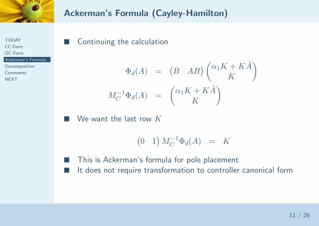
■ Continuing the calculation

Φd(A) =(

B AB)

(

α1K + KAK

)

M−1

CΦd(A) =

(

α1K + KAK

)

■ We want the last row K

(

0 1)

M−1

CΦd(A) = K

■ This is Ackerman’s formula for pole placement■ It does not require transformation to controller canonical form

Ackerman’s Formula - Pole Placement

TODAY

CC Form

OC Form


Decomposition

Comments

NEXT

12 / 26

■ Continuing with the design of the observer gains■ Find gain matrix B to place poles at -3 and -30.

A = AT =

(

−2 00 −3

)

B = CT =

(

−12

)

■ The desired characteristic equation is

Φd(s) = (s + 3)(s + 30) = s2 + 33s + 90

■ Φd(A) is given by

Φd(A) =

(

4 00 9

)

+ 33

(

−2 00 −3

)

+ 90

(

1 00 1

)

Φd(A) =

(

28 00 0

)


TODAY

CC Form

OC Form


Decomposition

Comments

NEXT

13 / 26

■ MC and M−1

Care given by

MC =(

B AB)

=

(

−1 22 −6

)

M−1

C=

(

−3 −1−1 −1/2

)

■ The observer gain matrix K = LT is given by

K =(

0 1)

M−1

CΦd(A)

=(

0 1)

(

−3 −1−1 −1/2

)(

28 00 0

)

=(

−1 −1/2)

(

28 00 0

)

K =(

28 0)


TODAY

CC Form

OC Form


Decomposition

Comments

NEXT

14 / 26

■ Check

K = LT =(

28 0)

L =

(

280

)

A − LC =

(

−2 00 −3

)

−

(

280

)

(

−1 2)

=

(

−2 00 −3

)

−

(

−28 480 0

)

=

(

−30 480 −3

)

■ (A − LC) is upper triangular. Eigenvalues on diagonal.■ Design goal achieved.

Kalman’s Decomposition

TODAY

CC Form

OC Form


Decomposition

Comments

NEXT

15 / 26

■ Not every state space realization is completely controllable orcompletely observable. Consider:

x1 = λ1x1 + u

x2 = λ2x2 + u

x3 = λ3x3

x4 = λ4x4

y = x1 + x3

A =

λ1 0 0 00 λ2 0 00 0 λ3 00 0 0 λ4

B =

1100

C =(

1 0 1 0)

D =(

0)

Which States are Controllable?

TODAY

CC Form

OC Form


Decomposition

Comments

NEXT

16 / 26

■ What does the controllability matrix tell us?

MC =(

B AB A2B A3B)

MC =

1 λ1 λ21

λ31

1 λ2 λ22

λ32

0 0 0 00 0 0 0

■ Only states x1 and x2 are controllable. (Range of MC)

Which States are Observable?

TODAY

CC Form

OC Form


Decomposition

Comments

NEXT

17 / 26

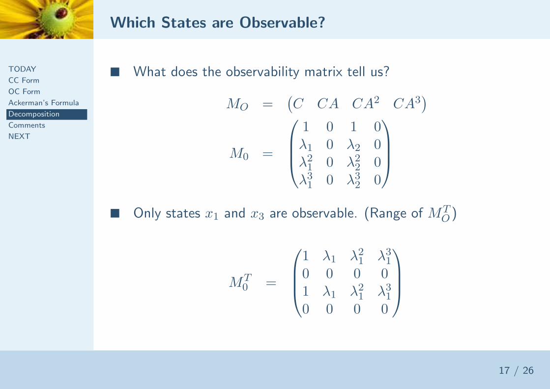
■ What does the observability matrix tell us?

MO =(

C CA CA2 CA3)

M0 =

1 0 1 0λ1 0 λ2 0λ2

10 λ2

20

λ31

0 λ32

0

■ Only states x1 and x3 are observable. (Range of MTO

)

MT0 =

1 λ1 λ21

λ31

0 0 0 01 λ1 λ2

1λ3

1

0 0 0 0

Kalman Decmoposition

TODAY

CC Form

OC Form


Decomposition

Comments

NEXT

18 / 26

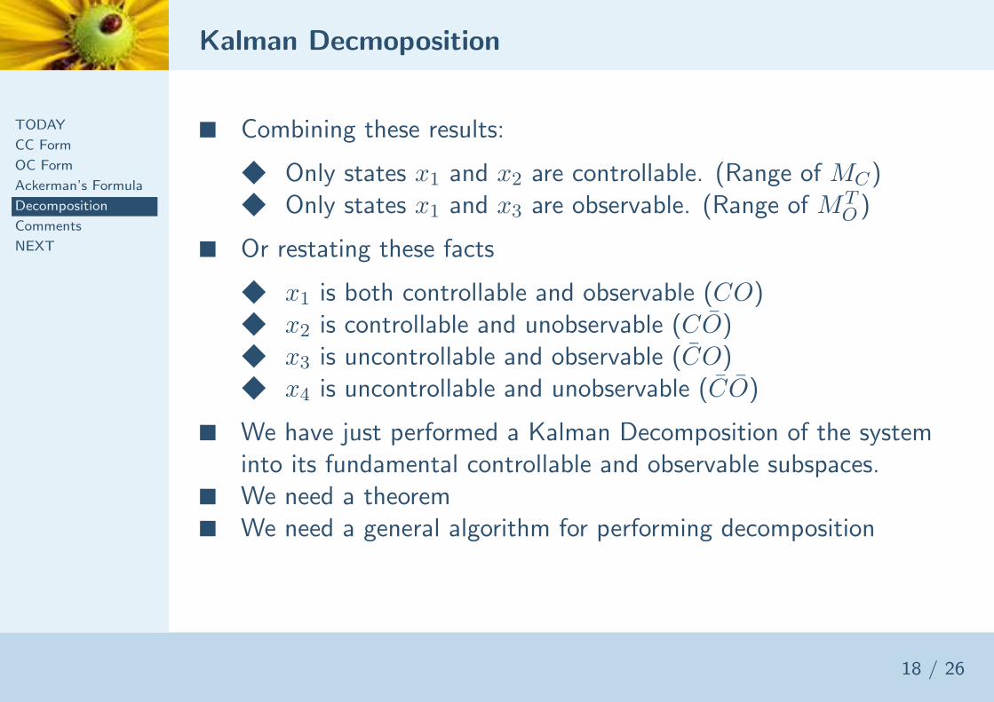
■ Combining these results:

◆ Only states x1 and x2 are controllable. (Range of MC)◆ Only states x1 and x3 are observable. (Range of MT

O)

■ Or restating these facts

◆ x1 is both controllable and observable (CO)◆ x2 is controllable and unobservable (CO)◆ x3 is uncontrollable and observable (CO)◆ x4 is uncontrollable and unobservable (CO)

■ We have just performed a Kalman Decomposition of the systeminto its fundamental controllable and observable subspaces.

■ We need a theorem■ We need a general algorithm for performing decomposition


TODAY

CC Form

OC Form


Decomposition

Comments

NEXT

19 / 26

THEOREM: (DeRusso, p 345)

■ If the controllability matrix associated with (A,B) has rankn1 (n1 < n), then there exists a matrix P such that x = Px thattransforms the original system into

(

˙xC

˙xC

)

=

(

AC A12

0 AC

)(

xC

xC

)

+

(

BC

0

)

u

y =(

CC CC

)

(

xC

xC

)

+ Du

■ where xC is n1 × 1 and represents the states that are CO, andxC is (n − n1) × 1and represents the states that are CO.


TODAY

CC Form

OC Form


Decomposition

Comments

NEXT

20 / 26

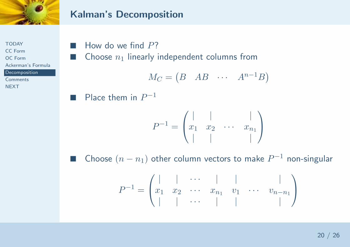
■ How do we find P?■ Choose n1 linearly independent columns from

MC =(

B AB · · · An−1B)

■ Place them in P−1

P−1 =

| | |x1 x2 · · · xn1

| | |

■ Choose (n − n1) other column vectors to make P−1 non-singular

P−1 =

| | · · · | | |x1 x2 · · · xn1

v1 · · · vn−n1

| | · · · | | |


TODAY

CC Form

OC Form


Decomposition

Comments

NEXT

21 / 26

■ Example

x =

(

−1 00 −1

)

x +

(

11

)

u

■ Controllability matrix MC

MC =

(

1 −11 −1

)

■ Place first column of MC into P−1

P−1 =

(

1 v11

1 v12

)

■ Let v = [1 0]T

P−1 =

(

1 11 0

)


TODAY

CC Form

OC Form


Decomposition

Comments

NEXT

22 / 26

■ Continuing˙x = PAP−1x + PBu

˙x =

(

−1 00 −1

)

x +

(

10

)

u

■ Which has the desired (controllable) decomposition■ We have a similar result for observability


TODAY

CC Form

OC Form


Decomposition

Comments

NEXT

23 / 26

THEOREM: (DeRusso, p 348)

■ If the observability matrix associated with (A,C) has rankn2 (n2 < n), then there exists a matrix P such that x = Px thattransforms the original system into

(

˙xO

˙xO

)

=

(

AO 0A21 A0

) (

xO

xO

)

+

(

BO

BO

)

u

y =(

CO 0)

x

(

xO

xO

)

+ Du

■ where xO is n2 × 1 and represents the states that are CO, andxO is (n − n2) × 1and represents the states that are CO.

■ Proof? Duality!!


TODAY

CC Form

OC Form


Decomposition

Comments

NEXT

24 / 26

■ In general, a realization can be partitioned into four subsets:

1. States which are controllable and observable2. States which are controllable but unobservable3. States which are uncontrollable but observable4. States which are both uncontrollable and unobservable

■ We will prove this result in Friday’s lecture lecture.

Comments

TODAY

CC Form

OC Form


Decomposition

Comments

NEXT

25 / 26

■ You now have used CC form to perform pole placement.■ You now have invoked duality and used Ackerman’s formula to

perform (full order) observer design.■ You’ve done one “eyeball” decomposition and have learned one

formal way of calculating a Kalman decomposition■ You now know how to calculate a controllable state space

realization and (partially) how to calculate an observable statespace realization

NEXT

TODAY

CC Form

OC Form


Decomposition

Comments

NEXT

26 / 26

■ NEXT:

◆ (Done) Lyapunov stability◆ (Done) Controller and Observer Canonical Forms, & Minimal

Realizations (DeRusso, Chap 6; Belanger, 3.7.6)◆ (Almost) Kalman’s Canonical Decomposition (DeRusso, 4.3

pp 200-203, 6.8; Belanger, 3.7.4)◆ (Some) Full state feedback & Observers (DeRusso, Chap 7;

Belanger, Chap 7)◆ LQR (Linear Quadratic Regulator) (Belanger, 7.4)◆ Kalman Filter (DeRusso, 8.9, Belanger 7.6.4)◆ Robustness & Performance Limitations (Various)

16.31 Fall 2005 Lecture Presentation Wed 26-Oct-05 ver 1web.mit.edu/16.31/www/...

Documents

Transcript of 16.31 Fall 2005 Lecture Presentation Wed 26-Oct-05 ver 1web.mit.edu/16.31/www/...