1458 IEEE TRANSACTIONS ON CIRCUITS AND SYSTEMS—I: …

1458 IEEE TRANSACTIONS ON CIRCUITS AND SYSTEMS—I: REGULAR PAPERS, VOL. 59, NO. 7, JULY 2012

Design of Fractional Delay Filter Using HermiteInterpolation Method

Chien-Cheng Tseng, Senior Member, IEEE, and Su-Ling Lee

Abstract—In this paper, the design of fractional delay (FD) filtersusing the Hermite interpolation is investigated. First, the transferfunction of fixed FD filters is obtained from the Hermite interpola-tion formula by using variable substitution. Then, two implemen-tationmethods for theHermite-based FD filters are presented. Oneis the derivative sampling scheme using an analog differentiator,the other is the Shannon sampling scheme with an auxiliary dig-ital differentiator. Next, the proposed method is applied to designwide-range variable fractional delay (VFD) filters and some exten-sions are made. Finally, several numerical examples are demon-strated to show the effectiveness of the proposed Hermite interpo-lation design method.

Index Terms—Digital filter, fractional delay, Hermite interpola-tion, Lagrange interpolation.

I. INTRODUCTION

I N RECENT years, fractional delay has become an impor-tant element in several applications like beam steering of

antenna arrays, time adjustment in digital receivers, modelingof music instruments, speech coding and synthesis, comb filterdesign and analog to digital conversion, etc. [1]–[14]. An ex-cellent survey of the fractional delay filter design is presentedin the tutorial paper [1]. The ideal frequency response of a frac-tional delay filter is given by

(1)

where is a positive real number in the desired range. Thus,the fractional-delay design problem is how to find a digital filtersuch that its actual frequency response fits the ideal response

as well as possible. When the delay is fixed, we aredealing with the so-called the fixed fractional delay (FFD) de-sign. The typical design methods include the window method[1], Lagrange interpolation method [1], discrete Fourier trans-form method [10], and maximally flat design at the frequency

[5]. If the delay is variable, it is called the variable frac-tional delay (VFD) design. So far, several methods have beenproposed to solve this design problem such as weighted least

Manuscript received February 20, 2011; revised May 25, 2011; accepted Oc-tober 12, 2011. Date of publication January 16, 2012; date of current versionJune 22, 2012. This work was supported by the National Science Council underContact NSC 100-2221-E-327-031-MY2. This paper was recommended by As-sociate Editor M. Mondin.C.-C. Tseng is with the Department of Computer and Communication Engi-

neering, National Kaohsiung First University of Science and Technology, Kaoh-siung 811, Taiwan (e-mail: [email protected]; [email protected]).S.-L. Lee is with the Department of Computer Science and Information

Engineering, Chung Jung Christian University, Tainan 711, Taiwan (e-mail:[email protected]).Digital Object Identifier 10.1109/TCSI.2011.2177136

squares (WLS) method [3], two-rate approach [27], and max-imally flat method [9], etc. These methods have their uniquefeatures.On the other hand, there exist various polynomial interpola-

tion methods in the numerical analysis in addition to the La-grange method [15], [16]. The first is the Newton approach, inwhich the interpolation polynomial is usually obtained by usinga divided difference table. The second is the Hermite method,where the interpolation polynomial not only matches the valuesof the function at various points butalso matches the first-order derivatives at . The third isthe spline interpolation method, in which the piecewise poly-nomials are used to fit the given sample points

under some smoothness constraints. Although theabove good interpolation methods have been successfully usedin the numerical analysis, the Hermite interpolation method hasnot been applied to design fractional delay filters, as done inthe Lagrange interpolation method. Thus, it is interesting to de-sign fractional delay filters based on the Hermite interpolationmethod. This is the main purpose of this paper.This paper is organized as follows. In Section II, the Hermite

polynomial interpolation method is applied to design fixed frac-tional delay filters. Two implementation methods are presented.One is the derivative sampling scheme using an analog differ-entiator, the other is the Shannon sampling scheme with an aux-iliary digital differentiator. In Section III, the Hermite method isextended to design wide-range variable fractional delay filters.The comparisons with conventional methods are made by usingthe application of adaptive time delay estimation. In Section IV,we further study the fractional delay filter design using the Her-mite method with second order derivative. Finally, conclusionsare drawn.

II. DESIGN OF FIXED FRACTIONAL DELAY FILTERS

In this section, the design of fixed fractional delay filters usingthe Hermite interpolation method is described in details, and theimplementation methods are studied.

A. Hermite Method

The Hermite interpolation method is de-scribed below: Given distinct points

and distinct firstorder derivatives ,then the polynomial of degree used to interpolate thesepoints has the form

(2)

1549-8328/$31.00 © 2012 IEEE

TSENG AND LEE: DESIGN OF FRACTIONAL DELAY FILTER USING HERMITE INTERPOLATION METHOD 1459

In order to let and besatisfied, the basis need to meet the following conditions:

(3)

where

(4)

with and . In [15], [16], ithas been shown that the basis satisfying the above condition isgiven by

(5a)

(5b)

where

(6)

and is the first order derivative of with respect to. Now, let us use the Hermite interpolation formula to designa fixed fractional delay filter. Taking , then the

points becomeand the derivatives become

. So, the Hermite poly-nomial becomes

(7)

where

(8a)

(8b)

Because at the interval , we have

(9)

Taking , the above equation can be rewritten in thefollowing form:

(10)

where

(11a)

(11b)

Using in (6), and , the above termcan be computed as

(12)

Now, to compute in (11a), the in (6) is rewrittenas

(13)

Using and , this equation can be expressedas

(14)

Thus, the derivative of is given by

(15)Based on this result, we have

(16)

Substituting (12) and (16) into (11a), we get

(17)

Obviously, is only the function of (not ), so wedenote

(18)


where

(19)

Moreover, substituting in (12) into (11b), we have

(20)

It can be observed that is only the function of (not), so we denote

(21)

Substituting (18) and (21) into (10), we have

(22)

Taking discrete-time Fourier transform at both sides, it yields

(23)

where and are the Fourier transforms ofand . Canceling , we get

(24)

Based on this result, two FIR filters are defined by

(25a)

(25b)

where filter coefficients and are obtained fromand by using window approach below:

(26)

with

otherwise(27)

Fig. 1. Derivative sampling scheme for the implementation of fractional delayfilter designed by Hermite interpolation method. The is the derivative of

.

The length of the window is . Note thatthe window interval and the center of thewindow should be close to the delay for reducing the trun-cation error caused by windowing. After the above choices, thefrequency response

(28)

will approximate the ideal response well.Moreover, the implementation complexity of two FIR filters

and is reported. If the direct-form realization isused, the number of adder and multiplier to implementand are and .So far, the Hermite interpolation design method has beendescribed. The remaining problem is how to implement thefractional delay filter in (28). This issue will be studied inSections II-B and II-C.

B. Implementation Using Derivative Sampling

In this subsection, the derivative sampling implementationmethod of the fixed fractional delay filter in (28) is presented.Fig. 1 shows a derivative sampling scheme implementing thefractional delay filter designed by using the Hermite interpola-tion method. The derivative sampling method was first investi-gated by Shannon in 1949 [17]. Then, several researchers alsostudied its properties. The details can be found in [18]–[21].Because is the first-order derivative of , it is easyto show that the frequency-domain relation between input andoutput in Fig. 1 is given by

(29)

where and are the Fourier transforms ofand . Thus, if two filters and in (25) are placedinto the block diagram in Fig. 1, then the output is the frac-tional delay sample of the input . Because the closed-formdesign is obtained in (18), (21) and (25), the filter coefficientsare easily computed. Now, let us use one numerical example tostudy the performance of the Hermite-based design method.1) Example 1: Now, one numerical example performed with

MATLAB language in an IBM PC compatible computer is used


Fig. 2. The designed results of fractional delay filter using Hermite methodfor various with step size 0.1. (a) Magnitude response, where linesalmost overlap together. (b) Group delay response.

to demonstrate the effectiveness of the proposed Hermite inter-polation method. To evaluate the performance, the normalizedroot mean square (NRMS) error is defined as

(30)

The above error is computed by using numerical rectangular in-tegration method with step size . Obviously, the smallerNRMS the error is, the better performance the designmethodhas. When the design parameters are chosen as ,

, and , Fig. 2(a) and (b) show themagnitude response and group delay of fractional delay filterdesigned by Hermite method for various with stepsize 0.1, that is, . Clearly, the specifica-tions are fitted well for various fractional delay values . Themagnitude responses in Fig. 2(a) almost overlap together, so wecan not see the differences among them. The above group delayresponse is computed with the following procedure:Step 1: Compute the unwrapped phase response by using the

MATLAB functions “angle” and “unwrap.”Step 2: Compute the negative derivative of the unwrapped

phase response by difference method and use it asthe final group delay response.

Moreover, the implementation complexity issue is addressed.Because , are chosen, thenumber of adders and multipliers needed to implement the twodigital filters and are 16 and 18. In [22], anotherderivative sampling method has been used to design a fractionaldelay filter whose filter coefficients are given by

(31a)

(31b)

Fig. 3. (a), (b) The magnitude response and group delay of fractional delayfilter designed by Hermite method. (c), (d) The magnitude response and groupdelay of fractional delay filter designed by the method in [22].

where . When the design parametersare chosen as , , and

, Fig. 3(a) and (b) show the magnitude re-sponse and group delay of a fractional delay filter designed byHermite method. The NRMS error of this design is 0.0040%.Fig. 3(c) and (d) show the magnitude response and group delayof a fractional delay filter designed by the method in [22]. TheNRMS error of this design is 3.7697% which is greater thanthe error of the Hermite method.Now, one remark about this implementation method is made.

In the derivative sampling implementation of Fig. 1, the deriva-tive signal is obtained by using a continuous-time (CT)differentiator. Usually, a CT differentiator is designed by usingoperational amplifiers, capacitors and resistors [24]. However,a CT differentiator is difficult to implement with high precision,so there can be errors in the frequency response of a CT differen-tiator. Now, let us study this error effect on the proposed designmethod. Without losing generality, we choose the distorted re-pose of a CT differentiator as

(32)

Using (28), the distorted fractional delay filter is then given by

(33)

When the design parameters are chosen as , ,, and , Fig. 4(a) and (b)

show the magnitude response and group delay of the designedfractional delay filter. The NRMS error in this design is8.0726%. It is clear that the performance of fractional delay fil-ters degrades if the frequency responses of CT differentiator dis-torts. In order to solve this distortion problem, the CT differen-tiator may be replaced by a discrete-time (DT) differentiator to


Fig. 4. (a), (b) The magnitude response and group delay of the designed frac-tional delay filter after considering the distorted CT differentiator.

Fig. 5. The block diagram that uses a discrete-time differentiator to implementthe fractional delay filter designed by Hermite interpolation method.

implement the proposed Hermite-based fractional delay filter.In Section II-C, this topic will be studied.

C. Implementation Using Digital Differentiator

Here, let us study another implementation that uses theShannon sampling scheme with an auxiliary digital first-orderdifferentiator. In Fig. 1, a continuous-time differentiator and asampler are used to obtain the derivative sample fromthe continuous-time signal . Thus, an interesting problemis to study whether we can obtain the derivative sampledirectly from the discrete-time signal by using a dis-crete-time first order differentiator. Fig. 5 shows a possible wayto achieve this purpose. The discrete-time differentiatoris designed to fit the ideal frequency response of the firstorder differentiator, that is,

(34)

After some manipulation, it is easy to show that the frequency-domain relation between and in Fig. 5 is given by

(35)

Fig. 6. (a), (b) The magnitude response and phase responseof the designed differentiator. (c), (d) The magnitude

response and group delay of the designed fractional delay filter for variousfractional delay values , 5.4, 5.6, and 5.8.

where and are the Fourier transforms ofand . Thus, if two filters and in (25) are placedinto the block diagram in Fig. 5, then the output is thefractional delay sample of the input .Now, one numerical example is illustrated below:1) Example 2: In this example, the weighted least squares

method with uniform weighting in [23] is first used to design astable IIR differentiator to approximate the ideal response

on the frequency band . The orders of thenumerator and denominator of IIR filter are equal to 30.Then, the transfer function of differentiator is chosen as

. Fig. 6(a) and (b) show the magnitude re-sponse and phase response of thedesigned differentiator. Clearly, fits ideal response wellon the frequency band . Moreover, the parameters arechosen as , , and .Fig. 6(c) and (d) show the magnitude response and group delayof the fractional delay filter

(36)

for various fractional delay values , 5.4, 5.6, and 5.8.From these results, it is clear that approximates the re-sponse well on the frequency band . Moreover,the differentiator and fractional delay filter almosthave the same bandwidth to fit the ideal response well, so we canuse the wideband differentiator to design a wideband frac-tional delay filter in (36). Finally, let us study the imple-mentation complexity of the designed fractional delay filter. Thenumber of adders and multipliers needed to implement the dig-ital differentiator is 60 and 61, and the number of addersand multipliers needed to implement the two filters and

is 16 and 18. Thus, the total number of adders and mul-tipliers needed to implement the designed fractional delay filter

is 76 and 79.


III. DESIGN OF VARIABLE FRACTIONAL DELAY FILTERS

In this section, the design of wide-range variable fractionaldelay (VFD) filter is first investigated. Then, the comparisonwith conventional designs is made.

A. Hermite VFD Filter Design

From (18), the coefficient in the Hermite design can berewritten as

(37)

where can be computed easily by using polynomial mul-tiplication. Moreover, from (21), the coefficient can berewritten as

(38)

where can be also calculated by using polynomial multi-plication. Using the (26) and (27) and substituting (37) and (38)into (25), two filters and can be written as

(39a)

(39b)

Substituting the above two filters into (28), the transfer functionof the variable fractional delay filter is given by

(40)

Fig. 7. The Farrow structure for implementing the Hermite-type variable frac-tional delay filter.

where subfilters are defined byand .

Based on (40), an efficient structure for implementing theHermite-type variable fractional delay filter is shown inFig. 7, where the fractional delay can be easily adjustedwithout redesigning the filter. This structure contains twoFarrow structures used in conventional VFD filter design[25]. The derivative signal can be obtained by usinga continuous-time or discrete-time differentiator. In whatfollows, the numerical examples are used to study these twoimplementation methods. To evaluate the performance of thevariable fractional delay filter design, the normalized rootmean square (NRMS) error is defined as

(41)where the interval is the desired variable range of thefractional delay. The double integrals in above (41) are com-puted by using a numerical rectangular integration method inwhich the step size of is and the step size of is

. Obviously, the smaller NRMS error is, the better per-formance the design method has. Now, one numerical exampleusing the derivative sampling scheme is studied below:1) Example 3: In this example, the design parameters are

chosen as , , , ,and . And the derivative sample is obtained byusing the derivative sampling scheme in Fig. 1. Fig. 8(a)–(d)show themagnitude response, group delay, magnitude error, andgroup delay error of a variable fractional delay filter designedby Hermite method. All figures are shown in the entire region

. From these results, it is clear that the designederrors are small for the Hermite design. The NRMS errorwith of this design is 0.1635%. Now, the implementationcomplexity in this example is reported. Because the number ofparameters used in digital filter is

and the number of parameters used in filter is


, the total number of parameterused in the proposed filter is 352.From the above example, it is clear that the delay of the

designed VFD filter can be adjusted in a wide range ,so the proposed filter is a wide-range VFD filter. The range

depends on the values of and . In ourexperience, the parameters and if

and are chosen. Althoughthe above VFD filter can be implemented by using the derivativesampling implementation method, this method needs a contin-uous-time differentiator. Now, let us study anther implementa-tion which uses a digital differentiator. In this case, the deriva-tive sample in Fig. 7 is obtained by passing the signal

through the first-order digital differentiator whoseresponse is defined by (34). The differentiator is usuallychosen as an FIR filter

(42)

where the filter coefficients satisfy the anti-symmetric conditionand . Thus, the frequency response of

can be written as

(43)

Using the least squares method, the optimal filter coefficientscan be obtained by minimizing the frequency response error inthe band [26]. Now, one example is studied below.2) Example 4: In this example, the design parameters are

chosen as , , , ,, , and . The magnitude response of the

first order differentiator designed by the least squares methodis shown in Fig. 9. Clearly, the approximation error is small inthe band . Fig. 10(a)–(d) show the magnitude response,group delay, magnitude error, and group delay error of a vari-able fractional delay filter designed by Hermite method. All fig-ures are shown in the entire region . Fromthese results, it is clear that the designed errors are small for theHermite design. The NRMS error with of this de-sign is 0.1387%. Now, the implementation complexity in thisexample is reported. The number of parameters used in filters

, , are ,, and , so the total

number of parameters used in the proposed filter is 372.

B. Comparison and Discussion

In [27]–[30], several good methods have been presented todesign VFD filters. In these methods, the adjustable range offractional delay is or where isa prescribed integer. Because the size of the adjustable range isalways equal to one, these methods are denoted as narrow-rangedesigns. In this paper, the adjustable range of the Hermite-basedVFD filter is , the range size of the proposed method isequal to . In examples 3 and 4, the range sizes are bothequal to 5. Thus, the proposed VFD filter is a wide-range design.From the experiment results, it is observed that the conventionalmethods in [27]–[30] have better performance than the proposed

Fig. 8. The designed results of variable fractional delay filter using deriva-tive scheme. (a) Magnitude response. (b) Group delay. (c) Magnitude error. (d)Group delay error.

method for the narrow-range design. This is because the conven-tional methods minimize the frequency response errors in band


Fig. 9. The magnitude response of first order differentiator designed by leastsquares method.

or to determine thefilter coefficients. Thus, these methods provide smaller designerrors. In this paper, the Hermite interpolation method is usedto determine the filter coefficients of the proposed VFD filter,so it provides a wide-range design. Therefore, it is unfair tocompare the narrow-range designs in [27]–[30] with proposedwide-range design because the specification is different. As weknown, some applications need a narrow-range VFD filter, andsome applications require a wide-range VFD filter. Thus, it ishard to say which is more important in the signal processingarea. For example, the image magnification application oftenneeds a narrow-range VFD filter [31], but the time-delay estima-tion application requires a wide-range VFD filter. To show howto apply the proposed wide-range VFD filter to the time-delayestimation problem, an estimation method is presented below.Given two received signals

(44a)

(44b)

where and are zero-mean white noises with vari-ance and , the problem is how to estimate the value oftime delay from the received signals and ,

. The delay is a noninteger and in the range. The block diagram of the proposed adaptive time-delay

estimation method is depicted in Fig. 11. Because the adjustablerange of the VFD filter is , the integer delay isplaced in the top branch of the block diagram to generate thedesired response below:

(45)

Let be the output obtained when passes throughthe digital differentiator in (42), then we have

(46)

Moreover, the output of the VFD filter can be written as

(47) Fig. 10. The designed results of variable fractional delay filter using a digitaldifferentiator. (a) Magnitude response. (b) Group delay. (c) Magnitude error.(d) Group delay error.


where is the output obtained when passes throughthe filter , and is the output obtained whenpasses through the filter . Thus, we have

(48a)

(48b)

Clearly, the output in (47) can be further rewritten as

(49)

where . The error between the desiredresponse and the VFD filter output is given by

(50)

In this paper, the delay is updated by the steepest descentalgorithm so that the mean square error is minimized,where the operator denotes expected value. The updatingequation is then given by

(51)

where is the step size. Let us use the instantaneous valueto replace its ensemble average value , then we have

(52)

where . Because and do notdepend on the parameter , the partial derivative term canbe computed by using (50):

(53)

Substituting (53) into (52), the updating equation reduces to

(54)

Finally, given the received signals and , the integer, the data length , the proposed adaptive time-delay algo-

rithm is summarized as follows:

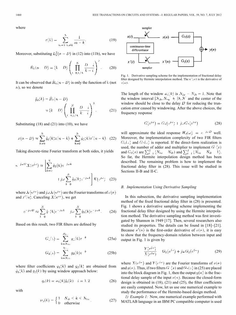
Fig. 11. The block diagram of the proposed adaptive time-delay estimationmethod.

Step 1: Set initial , step size , desired response, and time index .

Step 2: Use (46), (48), (49) to compute and .Step 3: Compute error .Step 4: Use (54) to calculate new delay and compute

the estimated value .Step 5: If , stop the iterative loop. Otherwise set

and go to step 2.So far, the adaptive time delay estimation method based on

the proposed wide-range VFD filter has been derived. Now, letus use a numerical example to demonstrate its effectiveness.1) Example 5: In this example, the received signals are given

by

(55a)

(55b)

where and are zero-mean Gaussian white noiseswith and . The data length is chosen as

. Two cases of delay are studied below:

(56a)

(56b)

The VFD filter is gotten from the designed results in example4, so the parameter . The step size is chosen as 0.3.Fig. 12(a) shows the learning curve in case 1. Clearly, thecurve converges to the true value 3.5 after 500 samples.Thus, the proposed algorithm can estimate the unknown timedelay correctly from the received signals. Fig. 12(b) showsthe learning curve in case 2. Clearly, the proposed adaptivealgorithm can track the time-delay change from 3.5 to 1.5 at

and change from 1.5 to 2.5 at . The largerstep size is, the faster tracking speed of adaptive algorithmhas. Finally, two remarks are made as follows:Remark 1: In case 1, time delay is a constant, so a two-

stage approach based on conventional narrow-range VFD filtercan be also used to estimate constant delay below:Stage 1:Use the cross correlation function between and

to get a coarse integer delay estimate .Stage 2:Use the narrow-range VFD filter to obtain a fractional

delay estimate . Then, the time delay can be esti-mated as .

However, the above narrow-range VFD filter method can notwork well if the delay is time-varying, that is, case 2. Fromexample 5, it is clear that the proposed wide-range adaptiveVFD filter method can work well in the cases of constant and


Fig. 12. The learning curves of adaptive time delay estimations. Thedashed lines are ideal curves. (a) Case 1. (b) Case 2.

time-varying delay , so the wide-range method is more suit-able than the narrow-range method in the application of time-varying delay estimation.Remark 2: Here, we first study how to extend two con-

ventional narrow-range methods to design a wide-range VFDfilter. One is the optimization method, the other is the Lagrangeclosed-form design. Then, these two methods are comparedwith the proposed Hermite method. Details are now describedbelow:Case 1: Optimization method

If the delay in (1) is equal to , the transfer functionof the conventional narrow-range VFD filter is usuallygiven by

(57)

where the subfilters are

(58)

When we choose and , then thefilter can be used to design a wide-range VFD

filter if the subfilters are determined byminimizingthe following error function:

(59)

From the Taylor series expansion, we know that thelarger range is, the larger orderneeds. That is, the adjustable range of delay can

be widen by increasing the number of subfilters .Although this design method provides a wide-range de-sign, it needs to solve the optimization problem in (59).The merit of the Hermite method is that it makes use ofa closed-form design. Thus, the Hermite method allowsto obtain the filter coefficients more easily than with theoptimization method.

Case 2: Lagrange closed-form designThe transfer function of the Lagrange VFD filter is givenby

(60)

where filter coefficients are

(61)

The above coefficient can be calculated by usingpolynomial multiplication. Substituting (61) into (60),we have Lagrange VFD filter below:

(62)

where . The delay incan be adjusted in the range , so it

is a wide-range design. Because the proposed Hermitemethod is an extension of the Lagrange method and usesthe derivative of the input signal, the Hermite methodwill provide smaller design error than the Lagrangemethod. Now, one example is used to compare theabove two methods with proposed method.

2) Example 6: In this example, we first present the results ofthe optimization method. In the design of VFD filter ,the parameters are chosen as , , ,

, , , and , so the adjustable rangeof delay is that is same as one in Example 4. TheNRMS error with of this design is 0.1204%, whichis slightly smaller than the error 0.1387% in example 4. And,the total number of parameters used in this filter is


which is same as one in Example 4. Fig. 13(a)shows the frequency response errorof the VFD filter in the optimization method. For comparison,Fig. 13(b) depicts the frequency response error

of the VFD filter in example 4. Clearly, the error dis-tributions of these two VFD filters are very different, so eachmethod has their unique features. Next, let us present the resultsof the Lagrange method. In the design of VFD filter ,the parameters are chosen as , , and

, so the adjustable range of delay is thatis same as one in Example 4. The NRMS error with ofthis design is 8.8035% which is larger than the error 0.1387%in example 4. And, the total number of parameters used in thisfilter is which is also larger than one inExample 4. Moreover, Fig. 13(c) shows the frequency responseerror of the VFD filter in the Lagrangemethod. Clearly, the errors in the high frequency band are largefor the Lagrange method. Thus, the Hermite method providesbetter design results than the Lagrange method because it usesthe information of the derivative of the input signal.

IV. EXTENSION DESIGN

The Lagrange design only considers the sampled value inorder to perform interpolation, and the Hermite design considersboth sampled value and first order derivative, so it is very nat-ural to study the interpolation that further considers the secondorder derivative. This extension case is investigated below:

A. Design Method

Given the distinct sampling points, distinct first order

derivatives ,and second order derivatives

, then thepolynomial of degree used to interpolate thesepoints has the form

(63)

In order to let , andbe satisfied, the basis need to meet the

following condition:

(64a)

(64b)

(64c)

where and . Now, let usassume that the solutions of three basis have the following form:

(65a)

Fig. 13. The absolute frequency response errors of the designed wide-rangeVFD filters. (a) Optimization method. (b) Hermite method. (c) Lagrangemethod.

(65b)

(65c)


where is the Lagrange basis in (6). Because three basis in(65) must satisfy the conditions in (64), it can be shown that

(66a)

(66b)

(66c)

(66d)

(66e)

Substituting (66) into (65), we obtain the three basis below:

(67a)

(67b)

(67c)

After the basis have been obtained, let us use the interpolationpolynomial in (63) to design the fractional delay filter. Because

at the sampling interval , we have

(68)

Taking and , (68) reduces to

(69)

where

(70a)

(70b)

(70c)

From (12) and (16), we have

(71a)

(71b)

where . Moreover, from(15), it can be shown that

(72)

Taking , (72) becomes

(73)

The notation “ ” denotes “define as.” Substituting (71) and (73)into (70), we get

(74a)

(74b)

(74c)

Substituting (74) into (69), we have

(75)

Taking the discrete-time Fourier transform at both sides, we ob-tain

(76)


Fig. 14. The designed results of extended Hermite method using first andsecond order derivatives. (a) Magnitude response. (b) Group delay response.

where , and are the Fouriertransforms of , and . Canceling , weget

(77)

From this result, if we define the three FIR filters below:

(78)

then the frequency response

(79)

will approximate the ideal response well.Now, let us study one numerical example of this design ap-proach.

B. Design Example

To evaluate the performance of this extended Hermite design,the normalized root mean square (NRMS) error is defined as

(80)

The above error is computed by using a numerical rectangularintegration method with step size . Obviously, thesmaller NRMS error is, the better performance the designmethod is. One example is presented below:1) Example 7: When the design parameters are chosen as

and , Fig. 14(a) and (b) show the magni-tude response and group delay of fractional delay filter designedwith this extended Hermite method where first and second order

derivatives are obtained with the derivative sampling scheme.The NRMS error of this design is 3.8 .Finally, one remark is made. From (74), it is easy to see that

the filter coefficients are all the polynomialof delay . Thus, we can get the variable fractional delay filterof this design easily by using polynomial multiplication. And,an efficient implementation with three Farrow structures can bealso obtained.

V. CONCLUSIONS

In this paper, the design of a fractional delay filter using theHermite interpolation has been presented. First, the details ofHermite interpolation to design fixed fractional delay filtershave been described. Then, two implementation methods forthe Hermite-based fractional delay filter have been presented.One is the derivative sampling scheme, the other is the Shannonsampling scheme with an auxiliary digital differentiator. Next,the proposed method has been applied to design a wide-rangeVFD filter and some extensions have been made. Finally, theadaptive time-delay estimation application example has beendeveloped to show the effectiveness of the proposed wide-rangeVFD filter. However, only the one-dimensional fractional delayfilter has been studied in this paper. Thus, it is interesting to ex-tend the proposed method to design two-dimensional fractionaldelay filters in the future.

REFERENCES[1] T. I. Laakso, V. Valimaki, M. Karjalainen, and U. K. Laine, “Split-

ting the unit delay: Tool for fractional delay filter design,” IEEE SignalProcess. Mag., vol. 44, pp. 30–60, Jan. 1996.

[2] S. C. Pei and C. C. Tseng, “A comb filter design using fractional sampledelay,” IEEE Trans. Circuits Syst. II, Analog Digit. Signal Process.,vol. 45, pp. 649–653, Jun. 1998.

[3] W. S. Lu and T. B. Deng, “An improved weighted least squares designfor variable fractional delay FIR filters,” IEEE Trans. Circuits Syst. II,Analog Digit. Signal Process., vol. 46, pp. 1035–1040, Aug. 1999.

[4] C. C. Tseng, “Design of 1-D and 2-D variable fractional delay all-pass filters using weighted least-squares method,” IEEE Trans. CircuitsSyst. I, Fundam. Theory Appl., vol. 49, pp. 1413–1422, Oct. 2002.

[5] S. C. Pei, P. H.Wang, and H. S. Lin, “Closed-form design of maximallyflat FIR fractional delay filter,” IEEE Signal Process. Lett., vol. 13, pp.405–408, Jul. 2006.

[6] T. B. Deng and Y. Lian, “Weighted-least-squares design of variablefractional-delay FIR filter using coefficient symmetry,” IEEE Trans.Signal Process., vol. 54, pp. 3023–3038, Aug. 2006.

[7] T. B. Deng, “Non-iterative WLS design of allpass variable fractional-delay digital filters,” IEEE Trans. Circuits Syst. I, Reg. Papers, vol. 53,pp. 358–371, Feb. 2006.

[8] T. B. Deng, “Coefficient-symmetries for implementing arbitrary-orderLagrange-type variable fractional-delay digital filters,” IEEE Trans.Signal Process., vol. 55, pp. 4078–4090, Aug. 2007.

[9] T. B. Deng, “Symmetric structures for odd-order maximally flat andweighted-least-squares variable fractional-delay filters,” IEEE Trans.Circuits Syst. I, Reg. Papers, vol. 54, pp. 2718–2732, Dec. 2007.

[10] C. C. Tseng and S. L. Lee, “Design of fractional delay FIR filter usingdiscrete Fourier transform interpolation method,” in Proc. IEEE Int.Symp. Circuits Syst., May 2008, pp. 1156–1159.

[11] J. J. Shyu and S. C. Pei, “A generalized approach to the design of vari-able fractional-delay FIR digital filters,” Signal Process., vol. 88, pp.1428–1435, Jun. 2008.

[12] J. J. Shyu, S. C. Pei, C. H. Chan, and Y. D. Huang, “Minimax design ofvariable fractional-delay FIR digital filters by iterative weighted least-squares approach,” IEEE Signal Process. Lett., vol. 15, pp. 693–696,2008.

[13] J. J. Shyu, S. C. Pei, and Y. D. Huang, “Two-dimensional Farrow struc-ture and the design of variable fractional-delay 2-D FIR digital filters,”IEEE Trans. Circuits Syst. I, Reg. Papers, vol. 56, pp. 395–404, Feb.2009.


[14] Y. D. Huang, S. C. Pei, and J. J. Shyu, “WLS design of variable frac-tional-delay FIR filters using coefficient relationship,” IEEE Trans.Circuits Syst. II, Exp. Briefs, vol. 56, pp. 220–224, Mar. 2009.

[15] C. J. Zarowski, An Introduction to Numerical Analysis for Electricaland Computer Engineering. Hoboken, NJ: Wiley, 2004.

[16] R. L. Burden and J. D. Faries, Numerical Analysis, 7th ed. PacificGrove, CA: Brooks/Cole, 2001.

[17] C. E. Shannon, “Communication in the presence of noise,” Proc. IRE,vol. 37, pp. 10–21, Jan. 1949.

[18] R. N. Bracewell, The Fourier Transform and Its Applications, 3rd ed.New York: McGraw-Hill, 2000.

[19] F. Marvasti, Nonuniform Sampling: Theory and Practice. Norwood,MA: Kluwer Academic, 2001.

[20] L. J. Fogel, “A note on the sampling theorem,” IRE Trans. Inf. Theory,vol. IT-1, pp. 47–48, Mar. 1955.

[21] D. A. Linden, “A discussion of sampling theorem,” Proc. IRE, vol. 47,no. 7, pp. 1219–1226, Jul. 1959.

[22] C. C. Tseng and S. L. Lee, “Design of wideband fractional delay filtersusing derivative sampling method,” IEEE Trans. Circuits Syst. I, Reg.Papers, vol. 57, pp. 2087–2098, Aug. 2010.

[23] W. S. Lu, S. C. Pei, and C. C. Tseng, “A weighted least-squares methodfor the design of stable 1-D and 2-D IIR digital filters,” IEEE Trans.Signal Process., vol. 46, pp. 1–10, Jan. 1998.

[24] A. S. Sedra and K. C. Smith, Microelectronic Circuits, 5th ed. NewYork: Oxford Univ. Press, 2004.

[25] C.W. Farrow, “A continuously variable digital delay element,” inProc.IEEE Int. Symp. Circuits Syst., May 1988, pp. 2641–2645.

[26] P. S. R. Diniz, E. A. da Silva, and S. L. Netto, Digital Signal Pro-cessing: System Analysis and Design. Cambridge, U.K.: CambridgeUniv. Press, 2002.

[27] E. Hermanowicz and H. Johansson, “On designing minimax adjustablewideband fractional delay FIR filters using two-rate approach,” inProc. Eur. Conf. Circuit Theory Design, Cork, Ireland, Aug.–Sep.29–1, 2005.

[28] J. Y. Kaakinen and T. Saramaki, “Multiplication-free polyno-mial-based FIR filters with an adjustable fractional delay,” Circuits,Syst., Signal Process., vol. 25, no. 2, pp. 265–294, Apr. 2006.

[29] J. Y. Kaakinen and T. Saramaki, “A simplified structure for FIR filterswith an adjustable fractional delay,” in Proc. IEEE Int. Symp. CircuitsSyst., May 2007, pp. 3439–3442.

[30] T. B. Deng, “Hybrid structures for low-complexity variable fractional-delay FIR filters,” IEEE Trans. Circuits Syst. I, Reg. Papers, vol. 57,no. 4, pp. 897–910, Apr. 2010.

[31] C. C. Tseng, “Closed-form design of half-sample delay IIR filter usingcontinued fraction expansion,” IEEE Trans. Circuits Syst. I, Reg. Pa-pers, vol. 54, no. 3, pp. 656–668, Mar. 2007.

Chien-Cheng Tseng (S’90–M’95–SM’01) wasborn in Taipei, Taiwan, in 1965. He received theB.S. degree (with honors) from Tatung Institute ofTechnology, Taipei, in 1988, and the M.S. and Ph.D.degrees from the National Taiwan University, Taipei,in 1990 and 1994, respectively, all in electricalengineering.From 1995 to 1997, he was an Associate Re-

search Engineer at Telecommunication Laboratories,Chunghwa Telecom Company, Ltd., Taoyuan,Taiwan. He is currently a Professor of the Depart-

ment of Computer and Communication Engineering, National KaohsiungFirst University of Science and Technology, Kaohsiung. His research interestsinclude digital signal processing, pattern recognition, quantum computation.He has over 100 published journal and conference papers in these fields.Dr. Tseng is currently an Editorial Board Member of IET Signal Processing,

a member of the Editorial Board of the EURASIP Signal Processing Journal,and a member of the Digital Signal Processing (DSP) Technical Committee ofthe IEEE Circuits and Systems Society. He was an Associate Editor of IEEETRANSACTIONS ON CIRCUITS AND SYSTEMS—PART I: REGULAR PAPERS from2010 to 2011. He was the recipient of research awards from the National ScienceCouncil in 1998, 1999, and 2001, the Paper Award from the Chinese ImageProcessing and Pattern Recognition Society of Taiwan in 1993, and the BestPaper Award from the Symposium of Telecommunications held in Taiwan in1994.

Su-Ling Lee was born in Tainan, Taiwan. She re-ceived the B.S., M.S., and Ph.D. degrees from theNational Tsing Hua University, Hsinchu, Taiwan in1986, 1989, and 1996, respectively, all in electricalengineering.From 1989 to 2006, she was an Associate Re-

search Engineer at Telecommunication Laboratories,Chunghwa Telecom Company, Ltd., Taoyuan,Taiwan. She is currently an Assistant Professor ofthe Department of Computer Science and Informa-tion Engineering, Chung-Jung Christian University,

Tainan. Her research interests include digital signal processing, image pro-cessing, and information and network security.

1458 IEEE TRANSACTIONS ON CIRCUITS AND SYSTEMS—I: …

Documents

Transcript of 1458 IEEE TRANSACTIONS ON CIRCUITS AND SYSTEMS—I: …