130 IEEE TRANSACTIONS ON IMAGE PROCESSING, …jwp2128/Papers/ZhouChenPaisleyetal2012.pdf ·...

130 IEEE TRANSACTIONS ON IMAGE PROCESSING, VOL. 21, NO. 1, JANUARY 2012

Nonparametric Bayesian Dictionary Learning forAnalysis of Noisy and Incomplete Images

Mingyuan Zhou, Haojun Chen, John Paisley, Lu Ren, Lingbo Li, Zhengming Xing, David Dunson,Guillermo Sapiro, and Lawrence Carin, Senior Member, IEEE

Abstract—Nonparametric Bayesian methods are considered forrecovery of imagery based upon compressive, incomplete, and/ornoisy measurements. A truncated beta-Bernoulli process is em-ployed to infer an appropriate dictionary for the data under testand also for image recovery. In the context of compressive sensing,significant improvements in image recovery are manifested usinglearned dictionaries, relative to using standard orthonormal imageexpansions. The compressive-measurement projections are alsooptimized for the learned dictionary. Additionally, we considersimpler (incomplete) measurements, defined by measuring asubset of image pixels, uniformly selected at random. Spatialinterrelationships within imagery are exploited through use of theDirichlet and probit stick-breaking processes. Several exampleresults are presented, with comparisons to other methods in theliterature.

Index Terms—Bayesian nonparametrics, compressive sensing,dictionary learning, factor analysis, image denoising, image inter-polation, sparse coding.

I. INTRODUCTION

A. Sparseness and Dictionary Learning

Recently, there has been significant interest in sparse imagerepresentations, in the context of denoising and interpolation[1], [13], [24]–[26], [27], [28], [31], compressive sensing (CS)[5], [12], and classification [40]. All of these applicationsexploit the fact that images may be sparsely represented in anappropriate dictionary. Most of the denoising, interpolation,and CS literature assume “off-the-shelf” wavelet and DCTbases/dictionaries [21], but recent research has demonstratedthe significant utility of learning an often overcomplete dictio-nary matched to the signals of interest (e.g., images) [1], [4],[12], [13], [24]–[26], [27], [28], [30], [31], [41].

Many of the existing methods for learning dictionaries arebased on solving an optimization problem [1], [13], [24]–[26],[27], [28], in which one seeks to match the dictionary to

Manuscript received April 17, 2010; revised April 19, 2011 and June 08,2011; accepted June 08, 2011. Date of publication June 20, 2011; date of currentversion December 16, 2011. This work was supported in part by DOE, by NSF,by ONR, by NGA, and by ARO. The associate editor coordinating the reviewof this manuscript and approving it for publication was Prof. Maya Gupta.

M. Zhou, H. Chen, J. Paisley, L. Ren, L. Li, Z. Xing, and L. Carin are with theDepartment of Electrical and Computer Engineering, Duke University, Durham,NC 27708-0291 USA.

D. Dunson is with the Department of Statistics, Duke University, Durham,NC 27708-0291 USA.

G. Sapiro is with the Department of Electrical and Computer Engineering,University of Minnesota, Minneapolis, MN 55455 USA.

Color versions of one or more of the figures in this paper are available onlineat http://ieeexplore.ieee.org.

Digital Object Identifier 10.1109/TIP.2011.2160072

the imagery of interest, while simultaneously encouraginga sparse representation. These methods have demonstratedstate-of-the-art performance for denoising, superresolution, in-terpolation, and inpainting. However, many existing algorithmsfor implementing such ideas also have some restrictions. Forexample, one must often assume access to the noise/residualvariance, the size of the dictionary is set a priori or fixedvia cross-validation-type techniques, and a single (“point”)estimate is learned.

To mitigate the aforementioned limitations, dictionarylearning has recently been cast as a factor-analysis problem,with the factor loading corresponding to the dictionary elements(atoms). Utilizing nonparametric Bayesian methods like thebeta process (BP) [29], [37], [42] and the Indian buffet process(IBP) [18], [22], one may, for example, infer the number offactors (dictionary elements) needed to fit the data. Further-more, one may place a prior on the noise or residual variance,with this inferred from the data [42]. An approximation to thefull posterior may be manifested via Gibbs sampling, yieldingan ensemble of dictionary representations. Recent research hasdemonstrated that an ensemble of representations can be betterthan a single expansion [14], with such an ensemble naturallymanifested by statistical models of the type described here.

B. Exploiting Structure and Compressive Measurements

In image analysis, there is often additional information thatmay be exploited when learning dictionaries, with this wellsuited for Bayesian priors. For example, most natural imagesmay be segmented, and it is probable that dictionary usagewill be similar for regions within a particular segment class.To address this idea, we extend the model by employing aprobit stick-breaking process (PSBP), with this generalizationof the Dirichlet process (DP) stick-breaking representation[34]. Related clustering techniques have proven successful inimage processing [26]. The model clusters the image patches,with each cluster corresponding to a segment type; the PSBPencourages proximate and similar patches to be included withinthe same segment type, thereby performing image segmentationand dictionary learning simultaneously.

The principal focus of this paper is on applying hierarchicalBayesian algorithms to new compressive measurement tech-niques that have been recently developed. Specifically, weconsider dictionary learning in the context of CS [5], [9], inwhich the measurements correspond to projections of typicalimage pixels. We consider dictionary learning performed“offline” based on representative (training) images, with thelearned dictionary applied within CS image recovery. We also

1057-7149/$26.00 © 2011 IEEE

ZHOU et al.: NONPARAMETRIC BAYESIAN DICTIONARY LEARNING FOR ANALYSIS OF IMAGES 131

consider the case for which the underlying dictionary is si-multaneously learned with inversion (reconstruction), with thisrelated to “blind” CS [17]. Finally, we design the CS projectionmatrix to be matched to the learned dictionary (when this isdone offline), and demonstrate, as in [12], that in practice, thisyields performance gains relative to conventional random CSprojection matrices.

While CS is of interest for its potential to reduce the numberof required measurements, it has the disadvantage of requiringthe development of new classes of cameras. Such cameras arerevolutionary and interesting [11], [35], but there have beendecades of previous research performed on development ofpixel-based cameras, and it would be desirable if such camerascould be modified simply to perform compressive measure-ments. We demonstrate that one may perform compressivemeasurements of natural images by simply sampling pixelsmeasured by a conventional camera, with the pixels uniformlyselected at random. This is closely related to recent research onmatrix completion [6], [23], [33], but here, we move beyondsimple low-rank assumptions associated with such previousresearch.

C. Contributions

This paper develops several hierarchical Bayesian models forlearning dictionaries for analysis of imagery, with applicationsin denoising, interpolation, and CS. The inference is performedbased on a Gibbs sampler, as is increasingly common in modernimage processing [16]. Here, we demonstrate how general-izations of the beta-Bernoulli process allow one to infer thedictionary elements directly based on the underlying degradedimage, without any a priori training data, while simultaneouslyinferring the noise statics and tolerating significant missingnessin the imagery. This is achieved by exploiting the low-dimen-sional structure of most natural images, which implies thatimage patches may be represented in terms of a low-dimen-sional set of learned dictionary elements. Excellent resultsare realized in these applications, including for hyperspectralimagery, which has not been widely considered in these settingspreviously. We also demonstrate how the learned dictionarymay be easily employed to define CS projection matrices thatyield markedly improved image recovery, as compared with themuch more typical random construction of such matrices.

The basic hierarchical Bayesian architecture developed hereserves as a foundation that may be flexibly extended to incor-porate additional prior information. As examples, we show herehow dictionary learning may be readily coupled with clustering,through the use of a DP [15]. We also incorporate spatial infor-mation within the image via a PSBP [32], with these extensionsyielding significant advantages for the CS application. The basicmodeling architecture may also exploit additional informationmanifested in the form of general covariates, as considered in arecent paper [43].

The remainder of the paper is organized as follows: InSection II, we review the classes of problems being considered.The beta-Bernoulli process is discussed in Section III, withrelationships made with previous work in this area, includingthose based on the IBP. The Dirichlet and PSBPs are discussedin Section IV, and several example results are presented in

Section V. Conclusions and a discussion of future work areprovided in Section VI, and details of the inference equationsare summarized in the Appendix.

II. PROBLEMS UNDER STUDY

We consider data samples that may be expressed in the fol-lowing form:

(1)

where , , and . The columns of matrixrepresent the components of a dictionary with

which is expanded. For our problem, the will correspondto (overlapped) pixel patches in an image [1], [13], [24],[25], [27], [42]. The set of vectors may be extractedfrom an image(s) of interest.

For the denoising problem, vectors may represent sensornoise, in addition to (ideally small) residual from representa-tion of the underlying signal as . To perform denoising, weplace restrictions on vectors , such that by itself doesnot exactly represent . A popular such restriction is thatshould be sparse, motivated by the idea that any particularmay often be represented in terms of a small subset of repre-sentative dictionary elements, from the full dictionary definedby the columns of . There are several methods that have beenrecently developed to impose such a sparse representation, in-cluding -based relaxation algorithms [24], [25], iterative al-gorithms [1], [13], and Bayesian methods [42]. One advantageof a Bayesian approach is that the noise/residual statistics maybe nonstationary (with unknown noise statistics). Specifically,in addition to placing a sparseness-promoting prior on , wemay also impose a prior on the components of . From the es-timated posterior density function on model parameters, eachcomponent of , corresponding to the th image patch,has its own variance. Given , our goal may be to si-multaneously infer and (and implicitly ), andthen, the denoised version of is represented as .

In many applications, the total number of pixels maybe large. However, it is well known that compression algorithmsmay be used on after the measurements have beenperformed, to significantly reduce the quantity of data that needbe stored or communicated. This compression indicates thatwhile the data dimensionality may be large, the underlyinginformation content may be relatively low. This has motivatedthe field of CS [5], [9], [11], [35], in which the total number ofmeasurements performed may be much less than . Towardthis end, researchers have proposed projection measurements ofthe following form:

(2)

where and , ideally with . The pro-jection matrix has traditionally been randomly constituted [5],[9], with a binary or real alphabet (and may be also a functionof the specific patch, and generalized as ). It is desirable thatmatrices and be as incoherent as possible.

The recovery of from is an ill-posed problem, unlessrestrictions are placed on . We may exploit the same classof restrictions used in the denoising problem; specifically, the


observed data satisfy , with and, and with sparse . Note that the sparseness con-

straint implies that (and hence, ) occupydistinct subspaces of , selected from the overall linear sub-space defined by the columns of .

In most applications of CS, is assumed known, corre-sponding to an orthonormal basis (e.g., wavelets or a DCT) [5],[9], [21]. However, such bases are not necessarily well matchedto natural imagery, and it is desirable to consider design ofdictionaries for this purpose [12]. One may even considerrecovering from while simultaneously in-ferring . Thus, we again have a dictionary-learning problem,which may be coupled with optimization of CS matrix , suchthat it is matched to (defined by a low coherence betweenthe rows of and columns of [5], [9], [12], [21]).

III. SPARSE FACTOR ANALYSIS WITH THE BETA-BERNOULLI

PROCESS

When presenting example results, we will consider threeproblems. For denoising, it is assumed that we measure

, where represents measurement noiseand model error; for the compressive-sensing application, weobserve , with and

; and finally, for the interpolation problem, we observe, where is a vector of elements from

contained within set . For all three problems, our objective isto infer underlying signal , with assumed sparse; wegenerally wish to simultaneously infer and . Toaddress each of these problems, we consider a statistical modelfor , placing Bayesian priors on , , and ;the way the model is used is slightly modified for each specificapplication. For example, when considering interpolation, onlythe observed are used within the model likelihoodfunction.

A. Beta-Bernoulli Process for Active-Set Selection

Let binary vector denote which of thecolumns of are used for representation of (active set);if a particular component of is equal to one, then thecorresponding column of is used in the representation of

. Hence, for data , there is an associated set oflatent binary vectors , and the beta-Bernoulli processprovides a convenient prior for these vectors [29], [37], [42].Specifically, consider the following model:

Bernoulli Beta

(3)where is the th component of , and and are modelparameters; the impact of these parameters on the model arediscussed below. Note that the use of product notation in (3) ismeant to denote that each component of and are indepen-dently drawn from distributions of the same form.

Considering limit , and after integrating out , thedraws of may be constituted as follows. For each ,draw Poisson and define , with

. Let represent the th component of , andfor . For , Bernoulli

, where ( represents the total numberof times the th component of is one). For

, we set . Note that asbecomes small, with increasing , it is probable that will besmall. Hence, with increasing , the number of new nonzerocomponents of diminishes. Furthermore, as a consequence ofBernoulli , when a particular component of vectors

is frequently one, it is more probable that it will beone for subsequent , . When , this construction for

corresponds to the IBP [18].Since defines which columns of are used to represent, (3) imposes that it is probable that some columns of are

repeatedly used among set , whereas other columnsof may be more specialized to particular . As demonstratedbelow, this has been found to be a good model whenare patches of pixels extracted from natural images.

B. Full Hierarchical Model

The hierarchical form of the model may now be expressed as

(4)

where represents the th component (atom) of , rep-resents the elementwise or Hadamard vector product,represents a identity matrix, and aredrawn as in (3). Conjugate hyperpriors Gamma and

Gamma are also imposed. The construction in (4),and with the prior in (3) for , is henceforth referred toas the BP factor analysis (BPFA) model. This model was firstdeveloped in [22], with a focus on general factor analysis; here,we apply and extend this construction for image-processing ap-plications.

Note that we impose independent Gaussian priors for andand for modeling convenience (conjugacy of consecutive

terms in the hierarchical model). However, the inferred poste-rior for these terms is generally not independent or Gaussian.The independent priors essentially impose prior informationabout the marginals of the posterior of each component,whereas the inferred posterior accounts for statistical depen-dence as reflected in the data.

To make connections of this model to more typical optimiza-tion-based approaches [24], [25], note that the negative loga-rithm of the posterior density function is

Gamma

Gamma Const (5)


where represents all unknown model parameters,, represents the

beta-Bernoulli process prior in (3), and represents modelhyperparameters (i.e., , , , , , and ). Therefore, thetypical constraints [24], [25] on the dictionary elementsand on the nonzero weights correspond here to the Gaussianpriors employed in (4). However, rather than employing an(Laplacian prior) constraint [24], [25] to impose sparseness on

, we employ the beta-Bernoulli process and .The beta-Bernoulli process imposes that binary should besparse and that there should be a relatively consistent (re)useof dictionary elements across the image, thereby also imposingself-similarity. Furthermore, and perhaps most importantly, wedo not constitute a point estimate, as one would do if a single

was sought to minimize (5). We rather estimate the fullposterior density , implemented via Gibbs sampling.A significant advantage of the hierarchical construction in (4)is that each Gibbs update equation is analytic, with detailed up-date equations provided in the Appendix. Note that consistentuse of atoms is encouraged because the active sets are definedby binary vectors , and these are all drawn from ashared probability vector ; this is distinct from drawing theactive sets independent and identically distributed (i.i.d.) from aLaplacian prior. Furthermore, the beta-Bernoulli prior imposesthat many components of are exactly zero, whereas witha Laplacian prior, many components are small but not exactlyzero (hence, the former is analogous to regularization, withthe latter closer to regularization).

IV. PATCH CLUSTERING VIA DIRICHLET AND PSBPS

A. Motivation

In the model previously discussed, each patch had a uniqueusage of dictionary atoms, defined by binary vector , which se-lects columns of . One may wish to place further constraintson the model, thereby imposing a greater degree of statisticalstructure. For example, one may employ that the cluster andthat within each cluster of each of the associated employ thesame columns of . This is motivated by the idea that a nat-ural image may be clustered into different types of textures orgeneral image structure. However, rather than imposing that all

within a given cluster use exactly the same columns of ,one may want to impose that all within such a cluster sharethe same probability of dictionary usage, i.e., that all withincluster share the same probability of using columns of , de-fined by , rather than sharing a single for all (as in theoriginal model above). Again, such clustering is motivated bythe idea that natural images tend to segment into different tex-tural or color forms. Below, we perform clustering in terms ofvectors , rather than explicit clustering of dictionary usage,which would entail cluster-dependent ; the “softer” nature ofthe former clustering structure is employed to retain model flex-ibility while still encouraging sharing of parameters within clus-ters.

A question when performing such clustering concerns thenumber of clusters needed, this motivating the use of nonpara-metric methods, like those considered in the next subsections.Additionally, since the aforementioned clustering is motivated

by the segmentations characteristic of natural images, it is desir-able to explicitly utilize the spatial location of each image patch,encouraging that patches in a particular segment/cluster arespatially contiguous. This latter goal motivates use of a PSBP,as also detailed as follows.

B. DP

The DP [15] constitutes a popular means of performing non-parametric clustering. A random draw from a DP, i.e.,DP , with precision and “base” measure , maybe constituted via the stick-breaking construction [34], i.e.,

(6)

where and Beta . The maybe viewed as a sequence of fractional breaks from a “stick” oforiginal length one, where the fraction of the stick broken offon break is . The are model parameters, associated withthe th data cluster. For our problem, it has proven effective toset Beta analogous to (3), andhence, . , drawn from , corresponds todistinct probability vectors for using the dictionary elements(columns of ). For sample , we draw , and a separatesparse binary vector is drawn for each sample , as

Bernoulli , with as the th component of . Inpractice, we truncate the infinite sum for the to elementsand impose , such that . A (conjugate)gamma prior is placed on the DP parameter .

We may view this DP construction as an “Indian buffet fran-chise, ” generalizing the Indian buffet analogy [18]. Specifi-cally, there are Indian buffet restaurants; each restaurantis composed of the same “menu” (columns of ) and is dis-tinguished by different probabilities for selecting menu items.The “customers” cluster based upon which restau-rant they go to. The represent the probability ofusing each column of in the respective different buffets.The cluster themselves among the different restau-rants in a manner that is consistent with the characteristics ofthe data, with the model also simultaneously learning the dic-tionary/menu . Note that we typically make truncationlarge, and the posterior distribution infers the number of clus-ters actually needed to support the data, as represented by howmany are of significant value. The model in (4), with theabove DP construction for , is henceforth referred toas DP-BPFA.

C. PSBP

The DP yields a clustering of , but it does not ac-count for our knowledge of the location of each patch withinthe image. It is natural to expect that if and are proximate,then, they are likely to be constituted in terms of similar columnsof .1 To impose this information, we employ the PSBP. A lo-gistic stick-breaking process is discussed in detail in [32]. Weemploy the closely related probit version here because it may

1Proximity can be modeled as in “spatial proximity,” as here developed indetail, or “feature proximity” as in nonlocal means and related approaches; see[26] and references therein.


be easily implemented in a Gibbs sampler. We note that whilethe method in [32] is related to that discussed below, in [32], theconcepts of learned dictionaries and beta-Bernoulli priors werenot considered. Another related model, which employs a probitlink function, is discussed in [7].

We augment the data as , where again repre-sents pixel values from the th image patch, and rep-resents the 2-D location of each patch. We wish to impose thatproximate patches are more likely to be composed of the sameor similar columns of . In the PSBP construction, all aspectsof (4) are retained, except for the manner in which are con-stituted. Rather than drawing a single -dimensional vector ofprobabilities , as in (3), we draw a library of such vectors, i.e.,

Beta (7)

and each is associated with a particular segment in the image.One is associated with location and drawn

(8)

with for all , and represents a pointmeasure concentrated at . Once is associated with a par-ticular , the corresponding binary vector is drawn as inthe first line of (3). Note that the distinction between DP andPSBP is that, in the former, mixture weights are in-dependent of spatial position , whereas the latter explicitly uti-lizes within (and below, we impose thatsmoothly changes with ).

The space-dependent weights are constructed as, where constitute

space-dependent probabilities. We set , and for, the are space-dependent probit functions, i.e.,

(9)where is a kernel characterized by parameter and

is a sparse set of real numbers. To implement thesparseness on , within prior , and(conjugate) Gamma , with set to favormost being large (if is large, draw is likelyto be near zero, such that most are near zero). Thissparseness-promoting construction is the same as that employedin the relevance vector machine (RVM) [39]. We here utilizeradial basis function kernel exp .

Each is encouraged to only be defined by a small setof localized kernel functions, and via the probit link function

, the probability is characterized by lo-calized segments over which the probability is contiguousand smoothly varying. The constitute a space-dependentstick-breaking process. Since , for all.

The PSBP model is relatively simple to implement within aGibbs sampler. For example, as indicated above, sparseness on

is imposed as in the RVM, and the probit link function issimply implemented within a Gibbs sampler (which is why itwas selected, rather than a logistic link function). Finally, wedefine a finite set of possible kernel parameters ,and a multinomial prior is placed on these parameters, with themultinomial probability vector drawn from a Dirichlet distri-bution [32] (each of the draws a kernel parameter from

). The model in (4), with the PSBP construction for, is henceforth referred to as PSBP-BPFA.

D. Discussion of Proposed Sparseness-Imposing Priors

The basic BPFA model is summarized in (4), and threerelated priors have been developed for sparse binary vectors

: 1) the basic truncated beta-Bernoulli process in(3); 2) a DP-based clustering of the underlying ; and3) a PSBP clustering of that exploits knowledgeof the location of the image patches. For 2 and 3, within aparticular cluster have similar , rather than exactly the samebinary vector; we also considered the latter, but this worked lesswell in practice. As discussed further when presenting results,for denoising and interpolation, all three methods yield com-parable performance. However, for CS, 2 and 3 yield markedimprovements in image-recovery accuracy relative to 1. Inanticipation of these results, we provide a further discussion ofthe three priors on and on the three image-processingproblems under consideration.

For the denoising and interpolation problems, we are pro-vided with data , albeit in the presence of noise andpotentially with substantial missing pixels. However, for thisproblem, may be made quite large since we may consider allpossible (overlapping) patches. A given pixel (apart fromnear the edges of the image) is present in different patches.Perhaps because we have such a large quantity of partially over-lapping data, for denoising and interpolation, we have foundthat beta-Bernoulli process in (3) is sufficient for inferring theunderlying relationships between the different dataand processing these data collaboratively. However, the beta-Bernoulli construction does not explicitly segment the image,and therefore, an advantage of the PSBP-BPFA constructionis that it yields comparable denoising and interpolation perfor-mance as (3) while also simultaneously yielding an effectiveimage segmentation.

For the CS problem, we measure , and therefore,each of the measurements associated with each image patch

loses the original pixels in (the projectionmatrix may also change with each patch, denoted by .Therefore, for CS, one cannot consider all possible shifts ofthe patches as the patches are predefined and fixed in the CSmeasurement (in the denoising and interpolation problems,the patches are defined in the subsequent analysis). There-fore, for CS imposition of the clustering behavior, via DP orPSBP provides important information, yielding state-of-the-artCS-recovery results.

E. Possible Extensions

The “Indian buffet franchise” and PSBP constructions con-sidered above and in the results below draw the -dimensional


probability vectors independently. This implies that withinthe prior, we impose no statistical correlation between the com-ponents of vectors and , for . It may be desir-able to impose such structure, imposing that there is a “global”probability of using particular dictionary elements, and the dif-ferent mixture components within the DP/PSBP constructionscorrespond to specific draws from global statistics of dictionaryusage. This will encourage the idea that there may be some“popular” dictionary elements that are shared across differentmixture components (i.e., popular across different buffets in thefranchise). One can impose this additional structure via a hier-archical BP (HBP) construction [37], related to the hierarchicalDP (HDP) [36]. Briefly, in an HBP construction, one may drawthe via the hierarchical construction, i.e.,

Beta

Beta (10)

where is the th component of . Vector constitutes“global” probabilities of using each of the dictionary ele-ments (across the “franchise”), and defines the probabilityof dictionary usage for the th buffet. This construction imposesstatistical dependences among vectors .

To simplify the presentation, in the following example results,we do not consider the HBP construction as good results have al-ready been achieved with the (truncated) DP and PSBP modelspreviously discussed. We note that in these analyses, the trun-cated versions of these models may actually help inference ofstatistical correlations among within the posterior (sincethe set is finite, and each vector is of finite length). If weactually considered the infinite limit on and on the numberof mixture components, inference of such statistical relation-ships within the posterior may be undermined because special-ized dictionary elements may be constituted across the differentfranchises, rather than encouraging sharing of highly similardictionary elements.

While we do not focus on the HBP construction here, a re-cent paper has employed the HBP construction in related dictio-nary learning for image-processing applications, yielding veryencouraging results [43]. We therefore emphasize that the basichierarchical Bayesian construction employed here is very flex-ible and may be extended in many ways to impose additionalstructure.

V. EXAMPLE RESULTS

A. Reproducible Research

The test results and the MATLAB code to reproduce themcan be downloaded from http://www.ee.duke.edu/~mz1/Re-sults/BPFAImage/.

B. Parameter Settings

For all BPFA, DP-BPFA, and PSBP-BPFA computations, thedictionary truncation level was set at orbased on the size of the image. Not all dictionary elements

are used in the model; the truncated beta-Bernoulli process in-fers the subset of dictionary elements employed to represent thedata . The larger the image, the more distinct typesof structure are anticipated and, therefore, the more dictionaryelements are likely to be employed; however, very similar re-sults are obtained with in all examples, just withmore dictionary elements are not employed for smaller images(therefore, to save computational resources, we setfor the smaller images). The number of DP and PSBP stickswas set at . The library of PSBP parameters is de-fined as in [32]; the PSBP kernel locations, i.e., , weresituated on a uniformly sampled grid in each image dimen-sion, situated at every fourth pixel in each direction (the re-sults are insensitive to many related definitions of ).The hyperparameters within the gamma distributions were setas , as is typically done in models ofthis type [39] (the same settings were used for the gamma priorfor DP precision parameter . The beta-distribution parametersare set as and if random initialization is used or

and if a singular value decomposition (SVD)based initialization is used. None of these parameters have beenoptimized or tuned. When performing inference, all parametersare randomly initialized (as a draw from the associated prior) orbased on the SVD of the image under test. The Gibbs samplersfor the BPFA, DP-BPFA, and PSBP-BPFA have been found tomix and quickly converge, producing satisfactory results with asfew as 20 iterations. The inferred images represent the averagefrom the collection samples. All software was written in nonop-timized MATLAB. On a Dell Precision T3500 computer with a2.4-GHz central processing unit, for patches ofsize with 20% of the RGB pixels observed at random,the BPFA required about 2 min per Gibbs iteration (the DP ver-sion was comparable), and PSBP-BPFA required about 3 minper iteration. For the 106-band hyperspectral imagery, whichemployed patches of size with 2% ofthe voxels observed uniformly at random, each Gibbs iterationrequired about 15 min.

C. Denoising

The BPFA denoising algorithm is compared with the orig-inal KSVD [13] and for both gray-scale and colored images.Newer denoising algorithms include block matching with 3-Dfiltering [8], the multiscale KSVD [28], and KSVD with thenonlocal mean constraints [26]. These algorithms assume thatthe noise variance is known, whereas the proposed model auto-matically infers, as part of the same model, the noise variancefrom the image under test. There are existing methods for esti-mation of the noise variance, as a preprocessing step, e.g., viawavelet shrinkage [10]. However, it was shown in [42] that thedenoising accuracy of methods like that in [13] can be sensi-tive to small errors in the estimated variance, which are likely tooccur in practice. Additionally, when doing joint denoising andimage interpolation, as we consider below, methods like that in[10] may not be directly applied to estimate the noise variance,as there is a large fraction of missing data. Moreover, the BPFA,DP-BPFA, and PSBP-BPFA models infer a potentially nonsta-tionary noise variance, with a broad prior on the variance im-posed by the gamma distribution.


TABLE IGRAY-SCALE IMAGE DENOISING PSNR RESULTS, COMPARING KSVD [13] AND BPFA, USING PATCH SIZE 8 � 8. THE TOP AND BOTTOM PARTS OF EACH

CELL ARE RESULTS OF KSVD AND BPFA, RESPECTIVELY

In the denoising examples, we consider the BPFA model in(3); similar results are obtained via the DP-BPFA and PSBP-BPFA models discussed in Section IV. To infer the final signalvalue at each pixel, we average the associated pixel contributionfrom each of the overlapping patches in which it is included(this is true for all results presented below in which overlappingpatches were used).

In Table I, we consider images from [13]. The proposed BPFAperforms very similarly to KSVD. As one representative ex-ample of the model’s ability to infer the noise variance, we con-sider the Lena image from Table I. The mean inferred noise stan-dard deviations are 5.83, 10.59, 15.53, 20.48, 25.44, 50.46, and100.54 for images contaminated by noise with the respectivestandard deviations of 5, 10, 15, 20, 25, 50, and 100. Each ofthese noise variances was automatically inferred using exactlythe same model, with no changes to the gamma hyperparam-eters (whereas for the KSVD results, it was assumed that thenoise variance was known exactly a priori).

In Table II, we present similar results, for denoising RGBimages; the KSVD comparisons come from [27]. An exampledenoising result is shown in Fig. 1. As another example of theBPFA’s ability to infer the underlying noise variance, for thecastle image, the mean (automatically) inferred variances are5.15, 10.18, 15.22, and 25.23 for images with additive noisewith true respective standard deviations of 5, 10, 15, and 25.The sensitivity of the KSVD algorithm to a mismatch betweenthe assumed and true noise variances is shown in [42, Fig. 1],and the insensitivity of BPFA to changes in the noise varianceand to requiring knowledge of the noise variance is deemed animportant advantage.

It is also important to note that the gray-scale KSVD results inTable I were initialized using an overcomplete DCT dictionary,whereas the RGB KSVD results in Table II employed an exten-sive set of training imagery to learn dictionary that was used

TABLE IIRGB IMAGE DENOISING PSNR RESULTS COMPARING KSVD [27] AND BPFA,BOTH USING A PATCH SIZE OF 7 � 7. THE TOP AND BOTTOM PARTS OF EACH

CELL SHOW THE RESULTS OF KSVD AND BPFA, RESPECTIVELY

to initialize the denoising computations. All BPFA, DP-BPFA,and PSBP-BPFA results employ no training data, with the dic-tionary initialized at random using draws from the prior or withthe SVD of the data under test.

D. Image Interpolation

For the initial interpolation examples, we consider standardRGB images, with 80% of the RGB pixels uniformly missingat random (the data under test are shown in Fig. 2). Results arefirst presented for the Castle and Mushroom images, with com-parisons between the BPFA model in (3) and the PSBP-BPFAmodel discussed in Section IV. The difference between the twois that the former is a “bag-of-patches” model, whereas the latteraccounts for the spatial locations of the patches. Furthermore,the PSBP-BPFA simultaneously performs image recovery andsegmentation. The results are shown in Fig. 3, presenting themean reconstructed images and inferred segmentations. Each


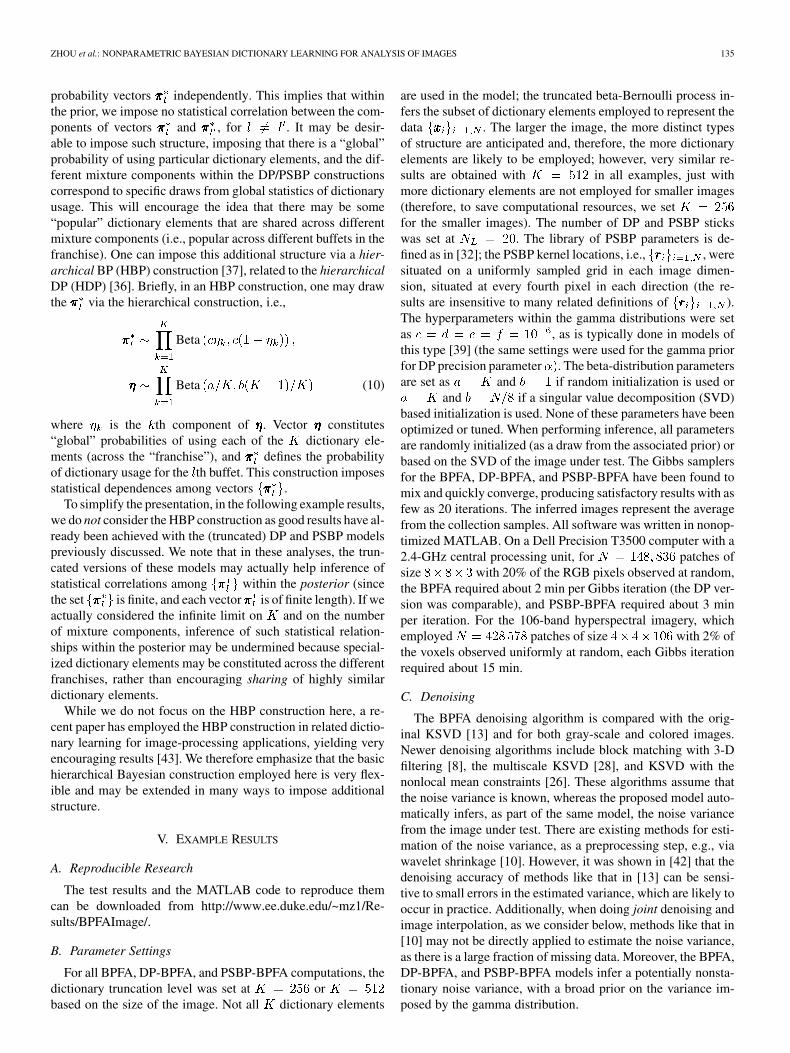
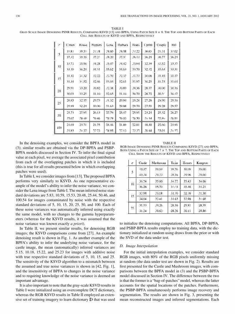
Fig. 1. (From left to right) The original horses image, the noisy horses image with the noise standard deviation of 25, the denoised image, and the inferreddictionary (from top left) with its elements ordered in the probability to be used. The low-probability dictionary elements are never used to represent �� and are drawn from the prior, showing the ability of the model to learn the number of dictionary elements needed for the data.

Fig. 2. Images with 80% of the RGB pixels missing at random. Although only20% of the actual pixels are observed, in these figures, the missing pixels areestimated based upon averaging all observed neighboring pixels within a 5 � 5spatial extent. (Left) Castle image (22.58-dB PSNR). (Right) Mushroom image(24.85 dB).

color in the inferred segmentation represents one PSBP mix-ture component, and the figure shows the last Gibbs iteration(to avoid issues with label switching between Gibbs iterations).While the BPFA does not directly yield a segmentation, its peaksignal-to-noise ratio (PSNR) results are comparable to those in-ferred by PSBP-BPFA, as summarized in Table III.

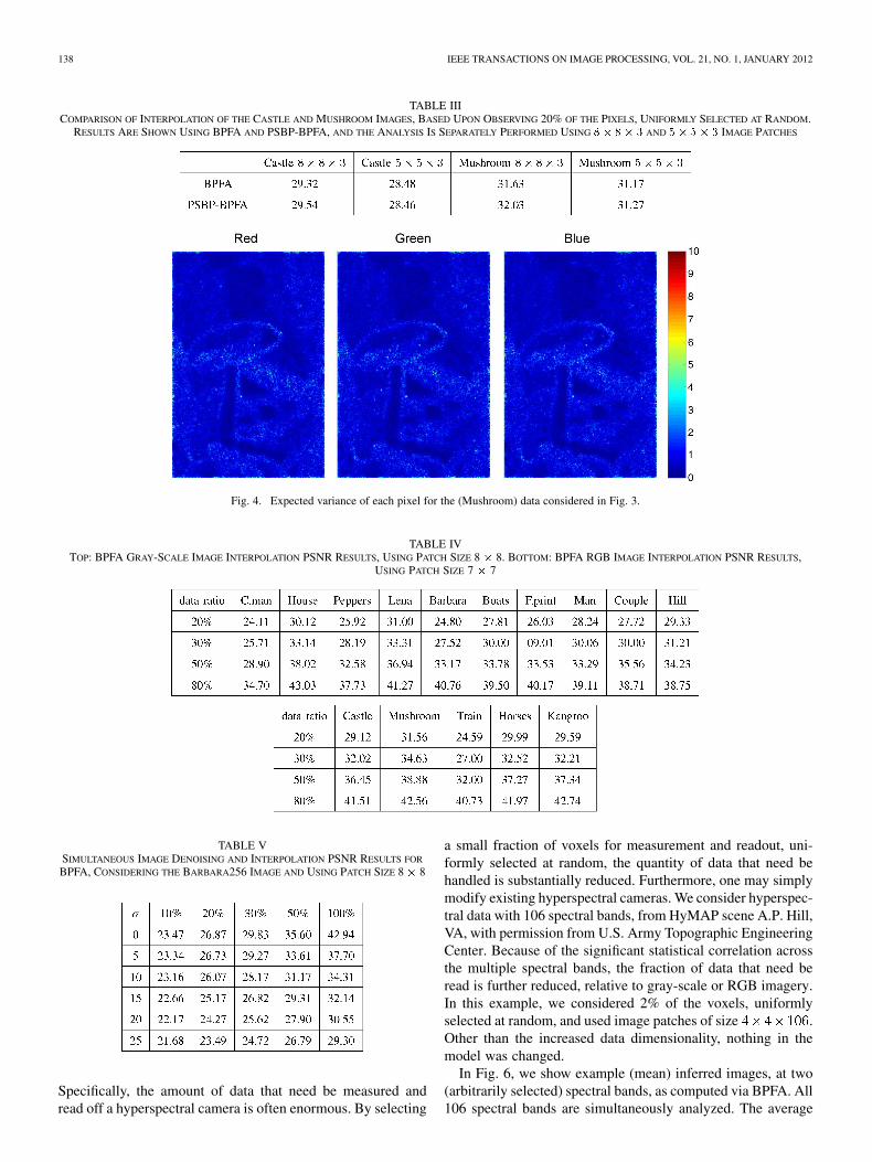
An important additional advantage of Bayesian models suchas BPFA, DP-BPFA, and PSBP-BPFA is that they provide ameasure of confidence in the accuracy of the inferred image.In Fig. 4, we plot the variance of the inferred error ,computed via the Gibbs collection samples.

To provide a more thorough examination of model perfor-mance, in Table IV, we present results for several well-studiedgray-scale and RGB images, as a function of the fraction ofpixels missing. All of these results are based upon BPFA, withDP-BPFA and PSBP-BPFA yielding similar results. Finally, inTable V, we perform interpolation and denoising simultane-ously, again with no training data and without prior knowledgeof the noise level (again, as previously discussed, it would bedifficult to estimate the noise variance as a preprocessing stepin this case using methods like that in [10] as, in this case, thereis also a large number of missing pixels). An example result isshown in Fig. 5. To our knowledge, this is the first time thatdenoising and interpolation have been jointly performed whilesimultaneously inferring the noise statistics.

Fig. 3. PSBP-BPFA analysis with 80% of the RGB pixels uniformly missingat random (see Fig. 2). The analysis is based on � � � � � image patches,considering all possible (overlapping) parches. For a given pixel, the results arethe average based upon all patches in which it is contained. For each example:(left) recovered image based on an average of Gibbs collection samples and(right) each color representing one of the PSBP mixture components.

For all of the examples previously considered, for both gray-scale and RGB images, we also attempted a direct application ofmatrix completion based on the incomplete matrix ,with columns defined by the image patches (i.e., for patches,with pixels in each, the incomplete matrix is of size ,with the th column defined by the pixels in ). We consideredthe algorithm in [20], using software from Prof. Candès’ web-site. For most of the examples previously considered, even aftervery careful tuning of the parameters, the algorithm diverged,suggesting that the low-rank assumptions were violated. For ex-amples for which the algorithm did work, the PSNR values weretypically 4 to 5 dB worse than those reported here for our model.

E. Interpolation of Hyperspectral Imagery

The basic BPFA, DP-BPFA, and PSBP-BPFA technologymay be also applied to hyperspectral imagery, and it is herewhere these methods may have significant practical utility.


TABLE IIICOMPARISON OF INTERPOLATION OF THE CASTLE AND MUSHROOM IMAGES, BASED UPON OBSERVING 20% OF THE PIXELS, UNIFORMLY SELECTED AT RANDOM.

RESULTS ARE SHOWN USING BPFA AND PSBP-BPFA, AND THE ANALYSIS IS SEPARATELY PERFORMED USING �� AND �� IMAGE PATCHES

Fig. 4. Expected variance of each pixel for the (Mushroom) data considered in Fig. 3.

TABLE IVTOP: BPFA GRAY-SCALE IMAGE INTERPOLATION PSNR RESULTS, USING PATCH SIZE 8 � 8. BOTTOM: BPFA RGB IMAGE INTERPOLATION PSNR RESULTS,

USING PATCH SIZE 7 � 7

TABLE VSIMULTANEOUS IMAGE DENOISING AND INTERPOLATION PSNR RESULTS FOR

BPFA, CONSIDERING THE BARBARA256 IMAGE AND USING PATCH SIZE 8� 8

Specifically, the amount of data that need be measured andread off a hyperspectral camera is often enormous. By selecting

a small fraction of voxels for measurement and readout, uni-formly selected at random, the quantity of data that need behandled is substantially reduced. Furthermore, one may simplymodify existing hyperspectral cameras. We consider hyperspec-tral data with 106 spectral bands, from HyMAP scene A.P. Hill,VA, with permission from U.S. Army Topographic EngineeringCenter. Because of the significant statistical correlation acrossthe multiple spectral bands, the fraction of data that need beread is further reduced, relative to gray-scale or RGB imagery.In this example, we considered 2% of the voxels, uniformlyselected at random, and used image patches of size .Other than the increased data dimensionality, nothing in themodel was changed.

In Fig. 6, we show example (mean) inferred images, at two(arbitrarily selected) spectral bands, as computed via BPFA. All106 spectral bands are simultaneously analyzed. The average


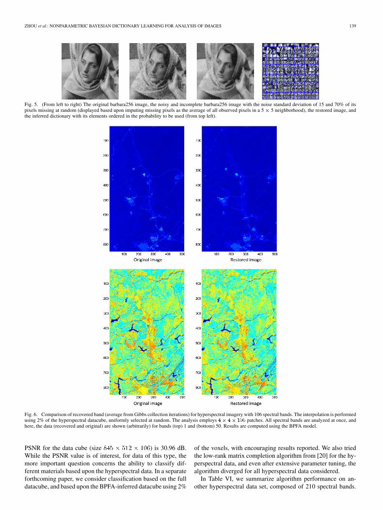
Fig. 5. (From left to right) The original barbara256 image, the noisy and incomplete barbara256 image with the noise standard deviation of 15 and 70% of itspixels missing at random (displayed based upon imputing missing pixels as the average of all observed pixels in a 5 � 5 neighborhood), the restored image, andthe inferred dictionary with its elements ordered in the probability to be used (from top left).

Fig. 6. Comparison of recovered band (average from Gibbs collection iterations) for hyperspectral imagery with 106 spectral bands. The interpolation is performedusing 2% of the hyperspectral datacube, uniformly selected at random. The analysis employs �� patches. All spectral bands are analyzed at once, andhere, the data (recovered and original) are shown (arbitrarily) for bands (top) 1 and (bottom) 50. Results are computed using the BPFA model.

PSNR for the data cube (size ) is 30.96 dB.While the PSNR value is of interest, for data of this type, themore important question concerns the ability to classify dif-ferent materials based upon the hyperspectral data. In a separateforthcoming paper, we consider classification based on the fulldatacube, and based upon the BPFA-inferred datacube using 2%

of the voxels, with encouraging results reported. We also triedthe low-rank matrix completion algorithm from [20] for the hy-perspectral data, and even after extensive parameter tuning, thealgorithm diverged for all hyperspectral data considered.

In Table VI, we summarize algorithm performance on an-other hyperspectral data set, composed of 210 spectral bands.


TABLE VIBPFA HYPERSPECTRAL IMAGE INTERPOLATION PSNR RESULTS. FOR THIS

EXAMPLE, THE TEST IMAGE IS A 150 � 150 URBAN IMAGE WITH 210SPECTRAL BANDS. RESULTS ARE SHOWN AS A FUNCTION OF THE PERCENTAGE

OF OBSERVED VOXELS, FOR DIFFERENT SIZED PATCHES (E.G., THE 4� 4 CASE

CORRESPONDS TO �� “PATCHES”)

We show the PSNR values as a function of percentage of ob-served data and as a function of the size of the image patch.Note that the 1 1 patches only exploit spectral information,whereas the other patch sizes exploit both spatial and spectralinformation.

F. CS

We consider a CS example in which the image is dividedinto 8 8 patches, with these constituting the underlyingdata to be inferred. For each of the blocks, avector of CS measurements is measured, where thenumber of projections per patch is , and the total number ofCS projections is . In our first examples, the elementsof are randomly constructed, as draws from ; manyother random projection classes may be considered [3] (andbelow, we also consider optimized projections , matchedto dictionary ). Each is assumed represented in termsof dictionary , and three constructions forwere considered: 1) a DCT expansion; 2) learning of usingBPFA, using training images; and 3) using the BPFA to per-form joint CS inversion and learning of . For 2, the trainingdata consisted of 4000 8 8 patches chosen at random from100 images selected from the Microsoft database (http://re-search.microsoft.com/en-us/projects/objectclassrecognition).The dictionary was set to , and the offline BP inferreda dictionary of size .

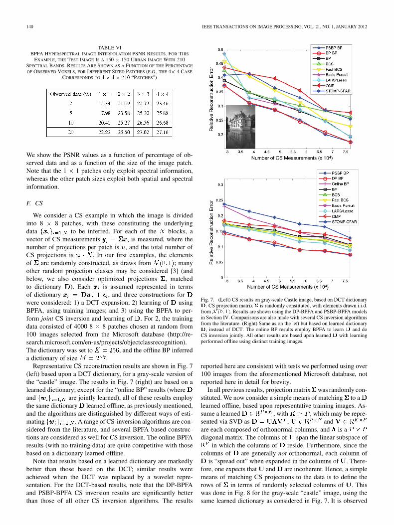
Representative CS reconstruction results are shown in Fig. 7(left) based upon a DCT dictionary, for a gray-scale version ofthe “castle” image. The results in Fig. 7 (right) are based on alearned dictionary; except for the “online BP” results (whereand are jointly learned), all of these results employthe same dictionary learned offline, as previously mentioned,and the algorithms are distinguished by different ways of esti-mating . A range of CS-inversion algorithms are con-sidered from the literature, and several BPFA-based construc-tions are considered as well for CS inversion. The online BPFAresults (with no training data) are quite competitive with thosebased on a dictionary learned offline.

Note that results based on a learned dictionary are markedlybetter than those based on the DCT; similar results wereachieved when the DCT was replaced by a wavelet repre-sentation. For the DCT-based results, note that the DP-BPFAand PSBP-BPFA CS inversion results are significantly betterthan those of all other CS inversion algorithms. The results

Fig. 7. (Left) CS results on gray-scale Castle image, based on DCT dictionary�. CS projection matrix �� is randomly constituted, with elements drawn i.i.d.from� �� . Results are shown using the DP-BPFA and PSBP-BPFA modelsin Section IV. Comparisons are also made with several CS inversion algorithmsfrom the literature. (Right) Same as on the left but based on learned dictionary�, instead of DCT. The online BP results employ BPFA to learn � and doCS inversion jointly. All other results are based upon learned� with learningperformed offline using distinct training images.

reported here are consistent with tests we performed using over100 images from the aforementioned Microsoft database, notreported here in detail for brevity.

In all previous results, projection matrix was randomly con-stituted. We now consider a simple means of matching to alearned offline, based upon representative training images. As-sume a learned , with , which may be repre-sented via SVD as ; andare each composed of orthonormal columns, and is adiagonal matrix. The columns of span the linear subspace of

in which the columns of reside. Furthermore, since thecolumns of are generally not orthonormal, each column of

is “spread out” when expanded in the columns of . There-fore, one expects that and are incoherent. Hence, a simplemeans of matching CS projections to the data is to define therows of in terms of randomly selected columns of . Thiswas done in Fig. 8 for the gray-scale “castle” image, using thesame learned dictionary as considered in Fig. 7. It is observed


Fig. 8. CS results on gray-scale Castle image, based on learned dictionary�(learning performed offline, using distinct training data). The projection matrix�� is matched to�, based upon an SVD of�.

that this procedure yields a marked improvement in CS recoveryaccuracy, for all CS inversion algorithms considered.

Concerning computational costs, all CS inversions were ef-ficiently run on personal computers, with the specifics compu-tational times dictated by the detailed MATLAB implementa-tion and the machine run on. A rough ranking of the compu-tational speeds, from fastest to slowest, is as follows: StOMP-CFAR, Fast BCS, OMP, BPFA, LARS/Lasso, Online BPFA,DP-BPFA, PSBP-BPFA, VB BCS, Basis Pursuit; in this list, al-gorithms BPFA through Basis Pursuits have approximately thesame computational costs.

The improved performance of the CS inversion based uponthe learned dictionaries is manifested as a consequence of thestructure that is imposed on the underlying image while per-forming inversion. The early CS inversion algorithms, of thetype considered in the above comparisons, imposed that the un-derlying image is sparsely represented in an appropriate basis(we showed results here based upon a DCT expansion of the 8

8 blocks over which CS inversion was performed, and similarresults were manifested using a wavelet expansion). The imposi-tion of such sparseness does not take into account the additionalstructure between the wavelet coefficients associated with nat-ural images. Recently, researchers have utilized such structureto move beyond sparseness and achieve even better CS-inver-sion quality [2], [19]; in this paper, structural relationships andcorrelations between basis-function coefficients are accountedfor. Additionally, there has been recent statistical research thathas moved beyond sparsity and that are of interest in the con-text of CS inversion [38]. In the tests, we omit, for brevity, thealgorithms in [2] and [19] yield performance that is comparableto the best results to the right in Fig. 7. Consequently, the im-position of structure in the form of learned dictionaries can beachieved using conventional basis expansions but with more so-phisticated inversion techniques, that account for structure inimagery. Therefore, the main advantage of the learned dictio-nary in the context of CS is that it provides a very convenient

means of defining projection matrices that are matched to nat-ural imagery, as done in Fig. 8. Once those projection matricesare specified, the CS inversion may be employed based upondictionaries as discussed here or based upon more traditionalexpansions (DCT or wavelets) and newer CS inversion methods[2], [19].

VI. CONCLUSION

The truncated beta-Bernoulli process has been employed tolearn dictionaries matched to image patches . Thebasic nonparametric Bayesian model is termed a BPFA frame-work, and extensions have been also considered. Specifically,the DP has been employed to cluster the , encour-aging similar dictionary-element usage within respective clus-ters. Furthermore, the PSBP has been used to impose that prox-imate patches are more likely to be similarly clustered (im-posing that they are more probable to employ similar dictio-nary elements). All inference has been performed by a Gibbssampler, with analytic update equations. The PBFA, DP-BPFA,and PSBP-BPFA have been applied to three problems in imageprocessing: 1) denoising; 2) image interpolation based upon asubset of pixels selected uniformly at random; and 3) learningdictionaries for CS and also CS inversion. We have also con-sidered jointly performing 1 and 2. Important advantages ofthe proposed methods are as follows. 1) A full posterior onmodel parameters are inferred, and therefore, “error bars” maybe placed on the inverted images. 2) The noise variance neednot be known; it is inferred within the analysis and may be non-stationary, and it may be inferred in the presence of significantmissing pixels. 3) While training data may be used to initializethe dictionary learning, this is not needed, and the BPFA resultsare highly competitive even based upon random initializations.In the context of CS, the DP-BPFA and PSBP-BPFA results arestate of the art, which is significantly better than existing pub-lished methods. Finally, based upon the learned dictionary, asimple method has been constituted for optimizing the CS pro-jections.

The interpolation problem is related to CS, in that we exploitthe fact that reside on a low-dimensional subspaceof , such that the total number of measurements is small rel-ative to (recall ). However, in CS, one employsprojection measurements , where , ideally with

. The interpolation problem corresponds to the specialcase in which the rows of are randomly selected rows of the

identity matrix. This problem is closely related to theproblem of matrix completion [6], [23], [33], where the incom-plete matrix has columns defined by .

While the PSBP-BPFA successfully segmented the imagewhile performing denoising and interpolation of missing pixels,we found that the PSNR performance of direct BPFA analysisperformed very close to that of PSBP-BPFA in those applica-tions. The use of PSBP-BPFA utilizes the spatial location ofthe image patches employed in the analysis, and therefore, itremoves the exchangeability assumption associated with thesimple BPFA (the location of the patches may be interchangedwithin the BPFA, without affecting the inference). However,since in the denoising and interpolation problems we have


many overlapping patches, the extra information provided byPSBP-BPFA does not appear to be significant. By contrast, inthe CS inversion problem, we do not have overlapping patches,and PSBP-BPFA provided significant performance gains rela-tive to BPFA alone.

APPENDIX

GIBBS SAMPLING INFERENCE

The Gibbs sampling update equations are given below; weprovide the update equations for the BPFA, and the DP andPSBP versions are relatively simple extensions. Below, rep-resents the projection matrix on the data, for image patch . Forthe CS problem, is typically fully populated, whereas for theinterpolation problem, each row of is all zeros, except for asingle one corresponding to the specific pixel that is measured.The update equations are the conditional probability of each pa-rameter, conditioned on all other parameters in the model.

Sample :

It can be shown that can be drawn from a normal distribu-tion as

with the covariance and mean expressed as

where

Sample :

Bernoulli

The posterior probability that is proportional to

and the posterior probability that is proportional to

Thus, can be drawn from a Bernoulli distribution as

Bernoulli (11)

Sample :

It can be shown that can be drawn from a normal distri-bution, i.e.,

(12)

with variance and mean expressed as

Note that is equal to either 1 or 0, and and canbe further expressed as

if

if

ifif .

Sample :

Beta aK

b(K-1)K Bernoulli

It can be shown that can be drawn from a Beta distributionas

Beta

Sample :

It can be shown that can be drawn from a Gamma distri-bution as


Sample :

(13)It can be shown that can be drawn from a Gamma distri-

bution as

(14)

Note that is a sparse identity matrix, is a diagonalmatrix, and is a sparse matrix; it is easy to find that onlybasic arithmetical operations are needed, and many unnecessarycalculations can be avoided, leading to fast computation and lowmemory requirement.

REFERENCES

[1] M. Aharon, M. Elad, and A. M. Bruckstein, “K-SVD: An algorithm fordesigning overcomplete dictionaries for sparse representation,” IEEETrans. Signal Process., vol. 54, no. 11, pp. 4311–4322, Nov. 2006.

[2] R. G. Baraniuk, V. Cevher, M. F. Duarte, and C. Hegde, “Model-basedcompressive sensing,” IEEE Trans. Inf. Theory, vol. 56, no. 4, pp.1982–2001, Apr. 2010.

[3] R. G. Baraniuk, “Compressive sensing,” IEEE Signal Process. Mag.,vol. 24, no. 4, pp. 118–121, Jul. 2007.

[4] A. M. Bruckstein, D. L. Donoho, and M. Elad, “From sparse solutionsof systems of equations to sparse modeling of signals and images,”SIAM Rev., vol. 51, no. 1, pp. 34–81, Jan. 2009.

[5] E. Candès and T. Tao, “Near-optimal signal recovery from random pro-jections: Universal encoding strategies?,” IEEE Trans. Inf. Theory, vol.52, no. 12, pp. 5406–5425, Dec. 2006.

[6] E. J. Candès and T. Tao, “The power of convex relaxation: Near-op-timal matrix completion,” IEEE Trans. Inf. Theory, vol. 56, no. 5, pp.2053–2080, May 2010.

[7] Y. Chung and D. B. Dunson, “Nonparametric Bayes conditional dis-tribution modeling with variable selection,” J. Amer. Stat. Assoc., vol.104, no. 488, pp. 1646–1660, Dec. 2009.

[8] K. Dabov, A. Foi, V. Katkovnik, and K. Egiazarian, “Image denoisingby sparse 3D transform-domain collaborative filtering,” IEEE Trans.Image Process., vol. 16, no. 8, pp. 2080–2095, Aug. 2007.

[9] D. L. Donoho, “Compressed sensing,” IEEE Trans. Inf. Theory, vol.52, no. 4, pp. 1289–1306, Apr. 2006.

[10] D. L. Donoho, I. M. Johnstone, G. Kerkyacharian, and D. Picard,“Wavelet shrinkage: Asymptopia,” J. Roy. Stat. Soc. B, vol. 57, no. 2,pp. 301–369, 1995.

[11] M. F. Duarte, M. A. Davenport, D. Takhar, J. N. Laska, T. Sun, K.F. Kelly, and R. G. Baraniuk, “Single-pixel imaging via compressivesampling,” IEEE Signal Process. Mag., vol. 25, no. 2, pp. 83–91, Mar.2008.

[12] J. M. Duarte-Carvajalino and G. Sapiro, “Learning to sense sparse sig-nals: Simultaneous sensing matrix and sparsifying dictionary optimiza-tion,” IEEE Trans. Image Process., vol. 18, no. 7, pp. 1395–1408, Jul.2009.

[13] M. Elad and M. Aharon, “Image denoising via sparse and redundantrepresentations over learned dictionaries,” IEEE Trans. Image Process.,vol. 15, no. 2, pp. 3736–3745, Dec. 2006.

[14] M. Elad and I. Yavneh, A Weighted Average of Sparse Representationsis Better Than the Sparsest One Alone 2010, Preprint.

[15] T. Ferguson, “A Bayesian analysis of some nonparametric problems,”Ann. Stat., vol. 1, no. 2, pp. 209–230, Mar. 1973.

[16] S. Geman and D. Geman, “Stochastic relaxation, Gibbs distributions,and the Bayesian restoration of images,” IEEE Trans. Pattern Anal.Mach. Intell., vol. PAMI-6, no. 6, pp. 721–741, Nov. 1984.

[17] S. Gleichman and Y. C. Eldar, Blind Compressed Sensing Tech-nion—Israel Inst. Technol., Haifa, Israel, CCIT Rep. 759, 2010,Preprint (on Arxiv.org).

[18] T. L. Griffiths and Z. Ghahramani, “Infinite latent feature models andthe Indian buffet process,” in Proc. Adv. Neural Inf. Process. Syst.,2005, pp. 475–482.

[19] L. He and L. Carin, “Exploiting structure in wavelet-based Bayesiancompressive sensing,” IEEE Trans. Signal Process., vol. 57, no. 9, pp.3488–3497, Sep. 2009.

[20] E. J. Candès, J.-F. Cai, and Z. Shen, “A singular value thresholdingalgorithm for matrix completion,” SIAM J. Optim., vol. 20, no. 4, pp.1956–1982, Jan. 2008.

[21] S. Ji, Y. Xue, and L. Carin, “Bayesian compressive sensing,” IEEETrans. Signal Process., vol. 56, no. 6, pp. 2346–2356, Jun. 2008.

[22] D. Knowles and Z. Ghahramani, “Infinite sparse factor analysis andinfinite independent components analysis,” in Proc. Int. Conf. Ind.Compon. Anal. Signal Separation, 2007, pp. 381–388.

[23] N. D. Lawrence and R. Urtasun, “Non-linear matrix factorizationwith Gaussian processes,” in Proc. Int. Conf. Mach. Learn., 2009, pp.601–608.

[24] J. Mairal, F. Bach, J. Ponce, and G. Sapiro, “Online dictionary learningfor sparse coding,” in Proc. Int. Conf. Mach. Learn., 2009, pp. 689–696.

[25] J. Mairal, F. Bach, J. Ponce, G. Sapiro, and A. Zisserman, “Super-vised dictionary learning,” in Proc. Neural Inf. Process. Syst., 2008,pp. 1033–1040.

[26] J. Mairal, F. Bach, J. Ponce, G. Sapiro, and A. Zisserman, “Non-localsparse models for image restoration,” in Proc. Int. Conf. Comput. Vis.,2009, pp. 2272–2279.

[27] J. Mairal, M. Elad, and G. Sapiro, “Sparse representation for colorimage restoration,” IEEE Trans. Image Process., vol. 17, no. 1, pp.53–69, Jan. 2008.

[28] J. Mairal, G. Sapiro, and M. Elad, “Learning multiscale sparse rep-resentations for image and video restoration,” SIAM Multisc. Model.Simul., vol. 7, no. 1, pp. 214–241, 2008.

[29] J. Paisley and L. Carin, “Nonparametric factor analysis with betaprocess priors,” in Proc. Int. Conf. Mach. Learn., 2009, pp. 777–784.

[30] R. Raina, A. Battle, H. Lee, B. Packer, and A. Y. Ng, “Self-taughtlearning: Transfer learning from unlabeled data,” in Proc. Int. Conf.Mach. Learn., 2007, pp. 759–766.

[31] M. Ranzato, C. Poultney, S. Chopra, and Y. Lecun, “Efficient learningof sparse representations with an energy-based model,” in Proc. NeuralInf. Process. Syst., 2006, pp. 1137–1144.

[32] L. Ren, L. Du, D. Dunson, and L. Carin, “The logistic stick breakingprocess,” J. Mach. Learn. Res., preprint.

[33] R. Salakhutdinov and A. Mnih, “Bayesian probabilistic matrix factor-ization using Markov chain Monte Carlo,” in Proc. Int. Conf. Mach.Learn., 2008, pp. 880–887.

[34] J. Sethuraman, “A constructive definition of Dirichlet priors,” Stat. Sin.,vol. 4, no. 2, pp. 639–650, 1994.

[35] M. Shankar, N. P. Pitsianis, and D. J. Brady, “Compressive videosensors using multichannel imagers,” Appl. Opt., vol. 49, no. 10, pp.B9–B17, Feb. 2010.

[36] Y. W. Teh, M. I. Jordan, M. J. Beal, and D. M. Blei, “HierarchicalDirichlet processes,” J. Amer. Stat. Assoc., vol. 101, no. 476, pp.1566–1581, Dec. 2006.

[37] R. Thibaux and M. I. Jordan, “Hierarchical beta processes and the In-dian buffet process,” in Proc. Int. Conf. Artif. Intell. Stat., 2007, pp.564–571.

[38] R. Tibshirani, M. Saunders, S. Rosset, J. Zhu, and K. Knight, “Sparsityand smoothness via the fused Lasso,” J. Roy. Stat. Soc. B., vol. 67, no.1, pp. 91–108, Feb. 2005.

[39] M. Tipping, “Sparse Bayesian learning and the relevance vector ma-chine,” J. Mach. Learn. Res., vol. 1, pp. 211–244, Jun. 2001.

[40] J. Wright, A. Y. Yang, A. Ganesh, S. S. Sastry, and Y. Ma, “Robustface recognition via sparse representation,” IEEE Trans. Pattern Anal.Mach. Intell., vol. 31, no. 2, pp. 210–227, Feb. 2009.

[41] J. Yang, J. Wright, T. Huang, and Y. Ma, “Image super-resolution viasparse representation,” IEEE Trans. Image Process., vol. 19, no. 11, pp.2861–2873, Nov. 2009.

[42] M. Zhou, H. Chen, J. Paisley, L. Ren, G. Sapiro, and L. Carin, “Non-parametric Bayesian dictionary learning for sparse image representa-tions,” in Proc. Neural Inf. Process. Syst., 2009, pp. 1–9.

[43] M. Zhou, H. Yang, G. Sapiro, D. Dunson, and L. Carin, “Dependenthierarchical beta process for image interpolation and denoising,” Proc.Int. Conf. Artificial Intelligence Statistics (AISTATS) JMLR W&CP,vol. 15, pp. 883–891, 2011.


Mingyuan Zhou received the B.Sc. degree inacoustics from Nanjing University, Nanjing, China,in 2005 and the M.Eng. degree in signal and infor-mation processing from the Chinese Academy ofSciences, Beijing, China, in 2008. He is currentlyworking toward the Ph.D. degree with the Depart-ment of Electrical and Computer Engineering, DukeUniversity, Durham, NC.

His current research interests include statisticalmachine learning and signal processing, with em-phasis on dictionary learning, sparse coding, and

image and video processing.

Haojun Chen received the M.S. and Ph.D. degrees inelectrical and computer engineering from Duke Uni-versity, Durham, NC, in 2009 and 2011, respectively.

His research interests include machine learning,data mining, signal processing, and image pro-cessing.

John Paisley received the B.S.E., M.S., and Ph.D. degrees from Duke Univer-sity, Durham, NC, in 2004, 2007, and 2010.

He is currently a Postdoctoral Researcher with the Department of ComputerScience, Princeton University, Princeton, NJ. His research interests includeBayesian nonparametrics and machine learning.

Lu Ren received the B.S. degree in electrical en-gineering from Xidian University, Xi’an, China, in2002 and the Ph.D. degree in electrical and computerengineering from Duke University, Durham, NC, in2010.

She is currently working with Yahoo! Lab as aScientist. Her research interests include machinelearning, data mining, and statistical modeling.

Lingbo Li received the B.Sc. degree in electronicinformation engineering with Xidian University,Xi’an, China, in 2008 and the M.Sc. degree insensing and signals with Duke University, Durham,NC, in 2010. She is currently working toward thePh.D. degree with the Department of Electrical andComputer Engineering, Duke University.

Her current research interests include statisticalmachine learning and signal processing, with em-phasis on dictionary learning and topic modeling.

Zhengming Xing received the B.S. degree intelecommunications from the Civil Aviation Uni-versity of China, Tianjin, China, in 2008 and theM.S. degree in electrical engineering from DukeUniversity, Durham, NC, in 2010. He is currentlyworking toward the Ph.D. degree in electrical andcomputer engineering with Duke University.

His research interests include statistical machinelearning, hyperspectral image analysis, compressivesensing, and dictionary learning.

David Dunson is currently a Professor of statisticalscience with Duke University, Durham, NC. Hisrecent projects have developed sparse latent factormodels that scale to massive dimensions and improveperformance in predicting disease and other pheno-types based on high-dimensional and longitudinalbiomarkers. Related methods can be used for com-bining high-dimensional data from different sourcesand for massively dimensional variable selection.His research interests include the development andapplication of novel Bayesian statistical methods

motivated by high-dimensional and complex data sets, with particular emphasison nonparametric Bayesian methods that avoid assumptions, such as normalityand linearity, and on latent factor models that allow dimensionality reductionin massively dimensional settings.

Dr. Dunson is a Fellow of the American Statistical Association and theInstitute of Mathematical Statistics. He was a recipient of the 2007 MortimerSpiegelman Award for the top public health statistician, the 2010 MyrtoLefkopoulou Distinguished Lectureship at Harvard University, and the 2010COPSS Presidents’ Award for the top statistician under 41.

Guillermo Sapiro was born in Montevideo,Uruguay, on April 3, 1966. He received his B.Sc.(summa cum laude), M.Sc., and Ph.D. degreesfrom Technion Israel Institute of Technology, Hafia,Israel, in 1989, 1991, and 1993, respectively.

After his postdoctoral research with Massachu-setts Institute of Technology, he became a memberof the Technical Staff with the research facilitiesof HP Labs, Palo Alto, CA. He is currently withthe Department of Electrical and Computer Engi-neering, University of Minnesota, where he holds the

position of a Distinguished McKnight University Professor and the VincentineHermes-Luh Chair in electrical and computer engineering.

Lawrence Carin (F’01–SM’96) was born on March 25, 1963 in Washington,DC. He received the B.S., M.S., and Ph.D. degrees in electrical engineering fromthe University of Maryland, College Park, in 1985, 1986, and 1989, respectively.

In 1989, he joined the Department of Electrical Engineering, Polytechnic Uni-versity, Brooklyn, Brooklyn, NY, as an Assistant Professor and, in 1994, becamean Associate Professor. In September 1995, he joined the Department of Elec-trical Engineering, Duke University, Durham, NC. He is now the William H.Younger Professor of engineering with Duke University. He is a Cofounder withSignal Innovations Group, Inc., which is a small business where he serves asthe Director of Technology. He is the author of over 200 peer-reviewed papers.His current research interests include signal processing, sensing, and machinelearning.

Dr. Carin is a member of the Tau Beta Pi and Eta Kappa Nu Honor Societies.

130 IEEE TRANSACTIONS ON IMAGE PROCESSING, …jwp2128/Papers/ZhouChenPaisleyetal2012.pdf ·...

Documents

Transcript of 130 IEEE TRANSACTIONS ON IMAGE PROCESSING, …jwp2128/Papers/ZhouChenPaisleyetal2012.pdf ·...