Economic cycles and their synchronization:A survey of spectral properties

L. Sellaa,b,∗, G. Vivaldoc, A. Grothd, M. Ghild,e

aDepartment of Economics “S. Cognetti de Martiis”, University of Turin, ItalybCNR-Ceris, Moncalieri (Turin), Italy

cIstituto Nazionale di Fisica Nucleare (INFN), Turin, ItalydEnvironmental Research & Teaching Institute and Geosciences Department, Ecole

Normale Superieure, Paris, FranceeDepartment of Atmospheric & Oceanic Sciences and Institute of Geophysics & Planetary

Physics, University of California, Los Angeles, CA 90095-1565, USA

Abstract

The present work applies several advanced spectral methods to the analysis ofmacroeconomic fluctuations in three countries of the European Union: Italy,The Netherlands, and the United Kingdom. We focus here in particular onsingular-spectrum analysis (SSA), which provides valuable spatial and frequencyinformation of multivariate data and that goes far beyond a pure analysis inthe time domain. The spectral methods discussed here are well established inthe geosciences and life sciences, but not yet widespread in quantitative eco-nomics. In particular, they enable one to identify and describe nonlinear trendsand dominant cycles — including seasonal and interannual components — thatcharacterize the deterministic behavior of each time series. These tools havealready proven their robustness in the application on short and noisy data, andwe demonstrate their usefulness in the analysis of the macroeconomic indicatorsof these three countries.

We explore several fundamental indicators of the countries’ real aggregateeconomy in a univariate, as well as a multivariate setting. Starting with individ-ual single-channel analysis, we are able to identify similar spectral componentsamong the analyzed indicators. Next, we consider combinations of indicatorsand countries, in order to take different effects of comovements into account.Since business cycles are cross-national phenomena, which show common char-acteristics across countries, our aim is to uncover hidden global behavior acrossthe European economies. Results are compared with previous findings on theU.S. indicators (Groth et al., 2012). Finally, the analysis is extended to includeseveral indicators from the U.S. economy, in order to examine its influence onthe European market.

∗Corresponding authorEmail addresses: lisa.sella@unito.it (L. Sella), gianna.vivaldo@unito.it (G.

Vivaldo), andreas.groth@ens.fr (A. Groth), ghil@lmd.ens.fr (M. Ghil)

Preprint submitted to — August 2, 2013

Keywords: Advanced spectral methods, European business cycle, Frequencydomain, Time domainJEL classification: C15, C60, E32

1. Introduction

The nature of aggregate fluctuations is one of the most controversial topicsin macroeconomics: the first systematic analysis of economic data from France,England, and the United States led Juglar (1862) to hypothesize a recurrentbehavior of economic crises, with strong mutual dependence between their ex-pansion and recession phases. About one and a half century later, the debateon the nature and causes of economic fluctuations is still going on, and somefundamental issues like the endogenous vs. the exogenous nature of businesscycles and their propagation mechanisms are still open (Kydland and Prescott,1982; Long and Plosser, 1983; King and Rebelo, 2000; Chiarella et al., 2005).

Although it is widely acknowledged that business cycles are multi-countryphenomena, showing common characteristics across countries (Woitek, 1996;Dickerson et al., 1998; Den Haan and Sumner, 2001; Stock and Watson, 2005;Mazzi and Savio, 2006), there is still no agreement on basic issues like thequantification of comovements, the existence of supranational cycles — e.g.,European or G7 ones — and the determinants of economic synchronization. Forthis reason, many theoretical and empirical studies suggest contrasting results,due to different data sets as well as different methodologies.

Concerning the mechanisms of economic synchronization, three main fac-tors have been identified theoretically, but hardly verified by empirical analysis.First of all, some scholars argue that economic and capital integration supportsthe creation of specialized production structures, due to which sector-specificshocks become region-specific (Krugman, 1993; Kalemli-Ozcan et al., 2001). Asa consequence, the business cycles of those countries showing similar productionpatterns would tend to converge (Imbs, 2004; Calderon et al., 2007); empiricalstudies (Otto et al., 2001; Baxter and Kouparitsas, 2005), however, are far frombuttressing this hypothesis.

Other scholars direct their attention on trade barriers, arguing that theirremoval enhances synchronization, because of the consequent transmission ofshocks in demand and because of knowledge and technological spillovers (Coeand Helpman, 1995; Frankel and Rose, 1998). Still, the effect of trade intensitieson business cycle comovements is empirically not clear (Gruben et al., 2002;Calderon et al., 2007; Baxter and Kouparitsas, 2005).

Finally, the impact of monetary and financial integration on synchronizationis theoretically ambiguous. On the one hand, monetary policies that are lessasymmetric, exchange rates that are more stable, and stronger trading relationsshould have a positive impact on synchronization (Inklaar and De Haan, 2001;De Haan et al., 2002). On the other hand, the fixed exchange rates could have anegative impact, since asymmetric shocks that may eventually occur cannot be

2

absorbed by exchange rate adjustments and are discharged on the real economy(De Haan et al., 2008).

The present work attempts to shed further light on supranational synchro-nization of business cycles, by applying recently developed spectral methods toa set of quarterly macroeconomic indicators — namely gross domestic product(GDP), consumption, fixed investment, export, and import — across three Eu-ropean countries. In the paper’s last part, the indicators of the U.S. economy areadded to the data set being analyzed, since this economy is strongly associatedand possibly coupled with the European ones.

Given that economic time series are rather short, highly volatile, and oftennonstationary, classical spectral estimation methods (e.g., the Fourier trans-form) are limited in their ability to describe the underlying dynamical behavior(Granger and Hatanaka, 1964; Granger, 1966, 1969). New developments in spec-tral estimation techniques, however, have been shown to successfully overcomethese limitations in many cases, and thus allow useful applications in variouseconomic contexts (Lisi and Medio, 1997; Higo and Nakada, 1998; Atesoglu andVilasuso, 1999; Baxter and King, 1999; A’Hearn and Woitek, 2001; Iacobucci,2003; Aadland, 2005). Moreover, these advanced spectral methods support aricher description of multivariate phenomena with respect to standard time-domain methods (Croux et al., 2001); this feature is particularly attractive inbusiness cycle analysis.

The multivariate, spectral approach presented in this paper is quite innova-tive in the field of economic research and extends the classical macroeconomicanalysis in the time domain to the frequency domain. Although fully exploitedin many fields of research, it has been so far mostly neglected in the analysis ofsocio-economic problems.

In the present work we propose the application of singular-spectrum analysis(SSA) to investigate multiple indicators, first in a univariate and, more impor-tantly, in a multivariate setting. SSA is well suited for the analysis of shortand noisy time series (Vautard et al., 1992; Ghil et al., 2002), like the typicalmacroeconomic ones. It is a nonparametric decomposition methodology and itdoes not require any a priori modeling of a time series to be analyzed. SSA al-lows a systematic description, quantification, and extraction of long-, medium-,and short-term components of the series being analyzed. Univariate SSA allowsus to investigate the behavior of each indicator separately, extracting the domi-nant periodic and quasi-periodic oscillations that account for most of the seriesvariability. On the other hand, the extension to multivariate SSA (M-SSA) givesdeeper insights into the common behavior of business fluctuations, both acrosscountries and across indicators.

The paper is divided into six sections: In Section 2, we introduce the dataset and pre-processing procedure. In Section 3, we present the methodology ofunivariate analysis, its multivariate extension, and a crucial significance test.In Section 4, we apply the method to individual time series, and then discussdifferent combinations thereof in Section 5. Finally, we draw conclusions aboutthe underlying macroeconomic dynamics and its synchronization in Section 6.

3

2. Data description and pre-processing

Our analysis is based on quarterly national accounts from Italy, the UnitedKingdom (henceforth UK), and The Netherlands 1. For each country we ana-lyze GDP at market prices, final consumption expenditure, gross fixed capitalformation, exports, and imports of goods and services 2.

The time series refer to the different time intervals of availability: they cover54 years for the UK (1955:01–2008:04, N = 216), 32 years for the Netherlands(1977:01–2008:04, N = 128), and 28 years for Italy (1981:01–2008:01, N = 112);hereN stands for the number of quarters. Figure 1 shows the raw time series andthe corresponding trend. The trend has been estimated by the Hodrick-Prescottfilter (Hodrick and Prescott, 1997), with the standard smoothing parameter forquarterly time series of λ = 1600. For normalization purposes, the trend wasextracted from the raw time series, the corresponding residuals were dividedby the trend, and then the relative residuals were standardized to the samevariance. Figure 2 illustrates this pre-processing procedure.

We selected the data from a set of European Union countries that show in-teresting characteristics, which could affect the features of business cycle prop-agation. First of all, The Netherlands are a small, wide-open economy, showingrelatively small GDP levels but very high shares of imports and exports.3 Conse-quently, they are more exposed to international shocks in comparison with Italyand the UK, two economies that are more closed. The UK has the economy thatis most strongly linked to that of the United States, while Italy’s most importanttrading partner is Germany.4 It is well known that bilateral trade represents achannel for the propagation of both international and country-specific shocks,and that it can favor synchronization among different economic systems.

Another significant characteristic of the UK economy is that it experiencesthe strongest fluctuations in GDP residuals. This is possibly due to the flexiblestructure of its labor market. In fact, the low bargaining power of its tradeunions allows more flexible adjustments in both wages and employment, thusdetermining more rapid responses to both positive and negative shocks, alongwith more sudden recessions and more pronounced expansions.

On the contrary, the high bargaining power of the Italian trade unions islikely to cause a more rigid reaction of the entire economy5. The Dutch econ-

1Quarterly national accounts are compiled in accordance with the European System ofAccounts (ESA95). Data are available from EUROSTAT on the web at http://epp.eurostat.ec.europa.eu/.

2All series are expressed in constant year-2000 Euros. They are seasonally adjusted andcorrected by working days, following the TRAMO-SEATS procedure (Maravall, 2005).

3In 2008, the ratio of imports to GDP was around 28% for Italy, 34% for the UK, and 77%for The Netherlands. The GDP share of exports was about 28%, 29%, and 84%, respectively.

4In 2000, the UK exported to the US 15.4% of its total exports and imported from it 13.2%of its total imports, while Italy exported 14.5% of its total to Germany and imported 17.7%from it, as derived from Feenstra et al. (2005).

5For instance, Italian Collective Agreements dictate very complex firing procedures forfirms that have more than 15 workers. As a consequence, both medium- and large-size firmsare discouraged from modifying their employment level.

4

omy shows a behavior that is intermediate between Italy and the UK, beingcharacterized by a labor market structure close to the Scandinavian typology(Esping-Andersen, 1999).

Finally, another important factor that differentiates among these three econo-mies is the availability of energy resources. While the UK and The Netherlandsboth have direct access to natural energy sources, Italy is a strong net importerof oil. Thus, energy supply shocks are likely to affect Italy much more stronglythan the other two countries, and hence induce larger business fluctuations. Asan example, zooming in on the HP trend of the Italian GDP in the 1970s andearly ’80s illustrates how the 1973 and 1979 energy shocks lengthened the Italianrecession phase in the early 1980s (not shown).

3. Methodology

SSA is a non-parametric method of time series analysis that provides insightinto the unknown or partially known dynamics of the underlying dynamicalsystem (Vautard and Ghil, 1989; Ghil and Vautard, 1991; Vautard et al., 1992).SSA allows the identification of different components of the analyzed signal —such as trends, oscillatory patterns, random noise — without the explicit needof a parametric model. The next three subsections, i.e. Sections 3.1–3.3, may beskipped, upon a first reading, by the student or researcher more interested in theresults than in the methodology. All three subsections are essential, however,for a full understanding of the results.

The starting point of SSA is the Mane-Takens idea to reconstruct dynamicsfrom a single time series by its time-delayed embedding (Mane, 1981; Takens,1981), and then to find a new orthogonal basis for the extended phase spaceso obtained that describes most of the variance in the original time series bya minimal number of components. As an optimal solution to this optimizationproblem, Broomhead and King (1986a) proposed the application of principalcomponent analysis (PCA).

In contrast to a classical Fourier decomposition, the new orthogonal basis isdata adaptive and not restricted to pure sine and cosine functions. This way,SSA provides a reconstruction of a skeleton of the dynamical system’s structurethat is formed by a few robust periodic orbits. Even when these simple attractorshave lost their stability, they still play a role in the observed patterns and leadto phase- and amplitude-modulated cycles.

3.1. Single-channel SSA

In this section, we start with a brief description of single-channel SSA. Givena time series {x(t), t = 1, ..., N} of length N , we build an M -dimensional phasespace by using M lagged copies of x

X

x(1) x(2) . . . x(M)x(2) x(3) . . . x(M + 1)

...... . . .

...x(N −M + 1) x(N −M + 2) . . . x(N)

. (1)

5

From this augmented time series X, we estimate the covariance matrix C =X′X/N ; here (·)′ denotes the transpose.

Due to finite-size effects for small N , C may deviate from symmetry; thus,we use the more accurate Toeplitz approach of Vautard and Ghil (1989), inwhich the entries cij of C are given by

cij =1

N − |i− j|

N−|i−j|∑t=1

x(t)x(t+ |i− j|). (2)

This formula yields constant entries cij along the (sub- and super)diagonals ofC, which depend only on the lag |i− j|.

Next, the symmetric covariance matrix is diagonalized

Λ = E′C E (3)

to yield a diagonal matrix Λ of eigenvalues λk and an orthogonal matrix E ofeigenvectors. The columns ek of E represent the new M -dimensional coordinatesystem and λk describes the variance of X in the direction of ek. Since theeigendecomposition in Eq. (3) is a similarity transformation of C, the varianceof the original time series x(t) is preserved in the eigenvalues, which now liealong the main diagonal of Λ.

From the largest eigenvalues we get a first impression of the most importantpart of the signal, which often can be separated from a tail of many small eigen-values. Further, in order to identify periodic or quasi-periodic behavior in theoriginal signal, Vautard and Ghil (1989) found that nearby eigenvalues at timesform a pair, with their variances being nearly equal, while the correspondingeigenvectors have the same period and are in phase quadrature. These so-called“oscillatory pairs” are the analog of sine-and-cosine pairs in Fourier analysis andadapt to the oscillations present in the system.

By projecting the time series x(t) onto each of the M eigenvectors ek, weget the M principal components (PCs),

ak(t) =

M∑j=1

x(t+ j − 1)ek(j), (4)

with 1 ≤ t ≤ N−M+1. The PCs are the projections of x onto the new basis; inthis case, the window width is M . For this reason, PCs exhibit no exact phaseinformation.

We are able, however, to study various aspects of the time series that belongto the direction ek by computing its reconstructed component (RC),

rk(t) =1

Mt

Ut∑j=Lt

ak(t− j + 1)ek(j), (5)

where (Mt, Lt, Ut) = (M, 1,M) for M ≤ t ≤ N −M + 1; for either end intervalthey are given in (Ghil et al., 2002). No information is lost during this recon-

struction process, since the sum of all individual RCs, x(t) =∑M

k=1 rk(t), givesthe original time series (Vautard et al., 1992).

6

3.2. Multi-channel SSAMultivariate SSA (M-SSA) is the extension of SSA to multivariate time series

(Broomhead and King, 1986b). It simultaneously analyses multiple channelsin order to identify and extract dominant spatio-temporal structures of theunderlying dynamics. In particular, M-SSA helps to extract oscillatory patternsthat are common to the time series at hand, even if they account for differentfractions of variance in each of the time series.

Given an L-channel vector time series x(t) = {xl(t) : l = 1, ..., L; t = 1, ..., N}of length N , its LM × LM grand covariance matrix C has the form

C1,1 C1,2 . . . C1,L

C2,1 C2,2 . . . C2,L

......

. . ....

CL,1 CL,2 . . . CL,L

. (6)

Each block Cl,l′ is a covariance matrix between channels l and l′ and is estimatedby

(Cl,l′)i,j =1

N

max{N,N+i−j}∑t=min{1,1+i−j}

xl(t)xl′(t+ i− j), (7)

where N = min{N,N + i− j} −max{1, 1 + i− j}+ 1 depends on the range ofsummation.

As in the univariate case, the grand covariance matrix is diagonalized into aset of LM eigenpairs {λk, ek} , k = 1 . . . LM . In contrast to the univariate case,M-SSA eigenvectors describe temporal as well as “spatial” correlations of themultivariate data set, where the L-dimensional space here is that of the vectorsx(t). Each eigenvector ek of length LM consists of L consecutive segments oflength M , denoted by ek = {elk(j) : l = 1 . . . L; j = 1 . . .M}. Each segment isassociated with an individual channel, and it describes the participation of thatchannel in a particular mode.

As in the univariate case, the corresponding PCs are obtained by projectingthe multivariate time series onto the eigenvectors

ak(t) =

L∑l=1

M∑j=1

xl(t+ j − 1)elk(j). (8)

This projection yields LM PCs of reduced length N −M + 1. Finally, it ispossible to reconstruct that part of channel l that correspond to eigenvector ek

by means of the RCs

rlk(t) =1

Mt

Ut∑j=Lt

ak(t− j + 1)elk(j), (9)

with k = 1, . . . , LM . The RCs have the same length N as the time series, withthe latter being completely reconstructed by the sum of all its RCs, xl(t) =∑LM

k=1 rlk(t).

7

3.3. Monte-Carlo SSA significance test

A critical step in all forms of spectral analysis is the distinction of significantoscillations from random fluctuations. The classical signal extraction approach,based on the identification of a gap in the spectrum of eigenvalues, has severallimitations: when either the signal-to-noise ratio decreases or the random fluc-tuations correlate, a separation into a few large eigenvalues and a remainingnoise floor becomes meaningless.

Thus, Allen and Smith (1996) have proposed a more stringent test; this testrelies on a more sophisticated null hypothesis, which takes the possibility of spu-rious oscillations into account. Based on a Monte-Carlo simulation technique,the extracted spectral components are tested against a red-noise hypothesis, i.e.an autoregressive process of order 1, AR(1),

X(t) = a1 [X (t− 1)−X0] + σξ(t) +X0; (10)

here X0 is the process mean and ξ a normally distributed white-noise processwith zero mean and unit variance.

Once the coefficients a1 and σ are estimated from the time series, an ensembleof surrogate time series is generated from the AR(1) process and compared withthe real data. In practice, this requires one to estimate the covariance matrixCR for each AR(1) realization and to project CR onto the eigenvectors E of theoriginal data

ΛR = E′CRE. (11)

Since Eq. (11) is not the eigendecomposition of the surrogate covariancematrix CR, the matrix ΛR is not necessarily diagonal, as it is in Eq. (3). In fact,this projection allows one to determine the degree of resemblance between thesurrogates generated by the test and the original data by computing statisticson the diagonal elements. From the ensemble distribution of λR along thediagonal, we are able to obtain significance intervals outside which the timeseries’ eigenvalues can be considered to be significantly different from an AR(1)process in Eq. (10). Note that a rejection of the most likely AR(1) process leadsto a rejection of all other red-noise processes, at the same or at an even higherlevel of significance (Ghil et al., 2002).

In the case of a multivariate data set, we follow the approach of Allen andRobertson (1996). Since the presence of cross-correlations would reduce thepower of the test, if not included in the null hypothesis, we first have to finda rotation that transforms the L channels to pairwise uncorrelated ones. Thisrotation can be simply achieved by a classical PCA, to which end we are ableto test the invariant set of eigenvalues against L independent AR(1) processes.This avoids the test against a vector AR(1) process, which may itself supportoscillations, the so-called principal oscillation patterns, or POPs (Penland, 1989;Von Storch, 1995). Having thus formulated the model in the null hypothesis,we proceed as in the univariate case: we first determine the covariance matrixfor every realization and then project it onto the M-SSA eigenvectors of therotated PCs. Finally, we test whether the M-SSA eigenvalues of the PCs exceeda preset significance level.

8

4. Individual analysis of macroeconomic indicators

In this section, we perform a univariate SSA analysis of all the indicatorsdiscussed in Section 2. To do so, we use the pre-processed data shown in Fig. 2and the SSA-MTM spectral toolkit developed at UCLA, which is available asfreeware at http://www.atmos.ucla.edu/tcd/ssa/.

The pre-processing is of the essence for the spectral analysis, since raw eco-nomic variables are typically characterized by a pervasive trend that dominatesthe shape of the power spectral estimate. This is reflected in a high peak at zerofrequency, which is scattered into the neighboring frequency bands due to leak-age effects (Granger, 1966). Figure 3 illustrates this effect on the GDP of theUK. After removing the trend with the help of the HP filter, the power spectraldensity (PSD) estimates in Fig. 3 reveal three distinct peaks, associated withperiodicities at about 9, 5, and 3 years. These spectral peaks suggest the pres-ence of roughly periodic components in the analyzed series, whose robustnessremains to be confirmed by further statistical tests.

In the next step, we carry out an SSA analysis of the trend residuals of theUK GDP. Figure 4 shows the spectrum of eigenvalues (filled circles) assigned toa frequency scale on the abscissa6.

The error bars represent the 2.5% and 97.5% quantiles of variance from anensemble of 1000 red noise realizations (cf. Section 3.3). Hence, it is veryunlikely that the eigenvalues lying outside the corresponding error bars areconsistent with the hypothesis of random fluctuations generated by a red-noiseprocess. In the case of the UK GDP, the eigenvalues 1–2 and 3–4 (filled circles)have more power than can be explained by simple red noise. The near-equalityof the two eigenvalues in each of these two pairs — in their size, as well as in thefrequency of the associated eigenmodes — suggests further that they representoscillatory pairs (Ghil et al., 2002).

Figure 4 indicates that the eigenvalue pair 1–2 is associated with a frequencyof approximately 5 years, which captures 39% of the variance in the detrendedand normalized time series. The pair 3–4 can be attributed to a 9-year oscil-lation, which describes 23% of the variance. Hence, almost two-thirds of thevariance is associated with the first four PCs of our SSA analysis. A possible3-year oscillation in the PSD estimation of Fig. 3 can be identified with theeigenvalue pair 7–8, but Fig. 4 shows that it cannot be distinguished from anAR(1) process at the 95% confidence level. Finally, note the oscillatory pair at a1-year periodicity, which clearly lies below the expected variance level. This canbe attributed to the elimination of the seasonal behavior in our pre-processing(cf. Section 2).

This comparison between the classical PSD estimation of Fig. 3 and the SSAestimates in Fig. 4 illustrates the capability of SSA to automatically identify

6Plotting the eigenvalues against their rank, as originally proposed by Vautard and Ghil(1989), is more useful in distinguishing between signal and noise. In identifying and statisti-cally testing for oscillatory modes, as we do here, it is more informative to plot the eigenvaluesversus the associated frequency of the corresponding eigenvectors (cf. Allen and Smith, 1996).

9

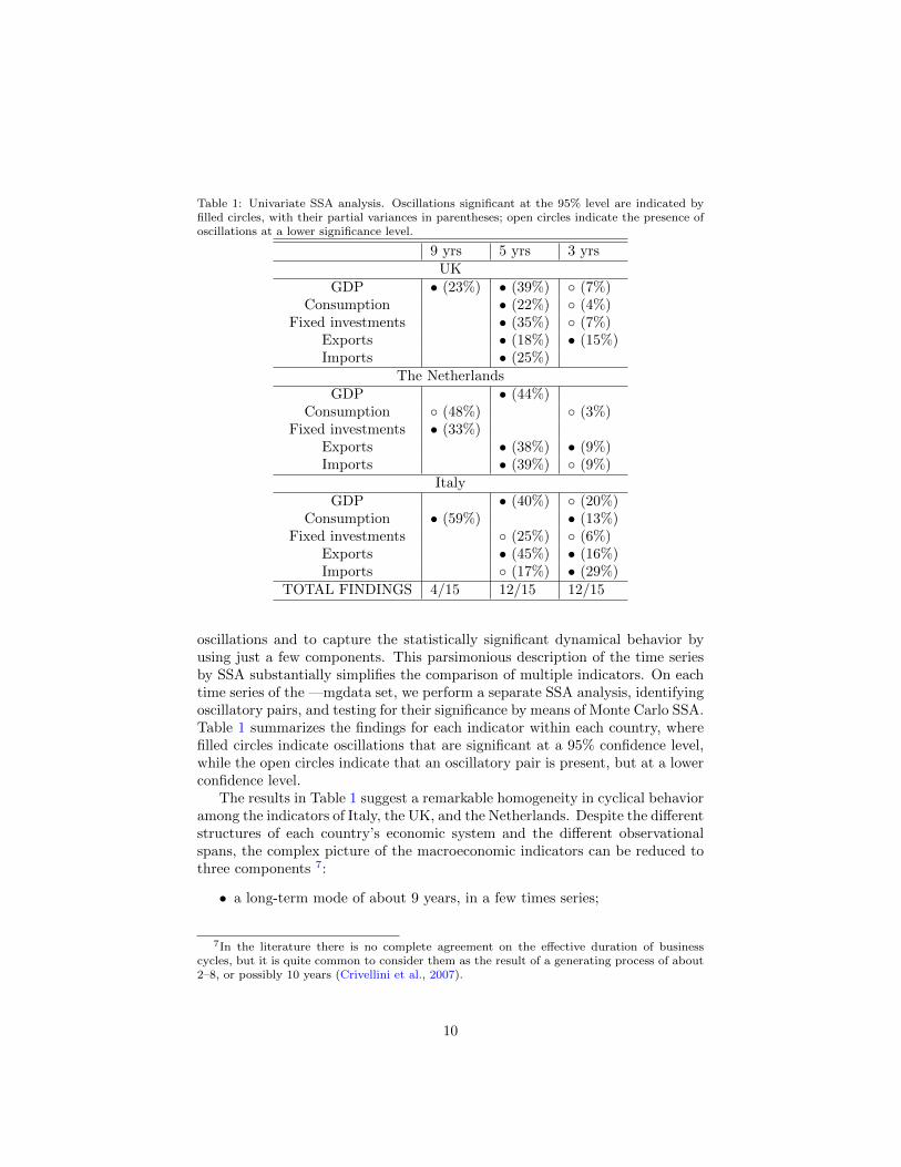
Table 1: Univariate SSA analysis. Oscillations significant at the 95% level are indicated byfilled circles, with their partial variances in parentheses; open circles indicate the presence ofoscillations at a lower significance level.

9 yrs 5 yrs 3 yrsUK

GDP • (23%) • (39%) ◦ (7%)Consumption • (22%) ◦ (4%)

Fixed investments • (35%) ◦ (7%)Exports • (18%) • (15%)Imports • (25%)

The NetherlandsGDP • (44%)

Consumption ◦ (48%) ◦ (3%)Fixed investments • (33%)

Exports • (38%) • (9%)Imports • (39%) ◦ (9%)

ItalyGDP • (40%) ◦ (20%)

Consumption • (59%) • (13%)Fixed investments ◦ (25%) ◦ (6%)

Exports • (45%) • (16%)Imports ◦ (17%) • (29%)

TOTAL FINDINGS 4/15 12/15 12/15

oscillations and to capture the statistically significant dynamical behavior byusing just a few components. This parsimonious description of the time seriesby SSA substantially simplifies the comparison of multiple indicators. On eachtime series of the —mgdata set, we perform a separate SSA analysis, identifyingoscillatory pairs, and testing for their significance by means of Monte Carlo SSA.Table 1 summarizes the findings for each indicator within each country, wherefilled circles indicate oscillations that are significant at a 95% confidence level,while the open circles indicate that an oscillatory pair is present, but at a lowerconfidence level.

The results in Table 1 suggest a remarkable homogeneity in cyclical behavioramong the indicators of Italy, the UK, and the Netherlands. Despite the differentstructures of each country’s economic system and the different observationalspans, the complex picture of the macroeconomic indicators can be reduced tothree components 7:

• a long-term mode of about 9 years, in a few times series;

7In the literature there is no complete agreement on the effective duration of businesscycles, but it is quite common to consider them as the result of a generating process of about2–8, or possibly 10 years (Crivellini et al., 2007).

10

• an intermediate 5-year oscillation, in nearly all indicators; and

• a faster oscillation of about 3 years, accounting for a small fraction of thetotal variance.

As already mentioned at the beginning of Section 3, a few robust periodicorbits can generate phase- and amplitude-modulated oscillations in the observedtime series. This behavior can be reconstructed, to some extent, by using theRCs. As an example, in Fig. 5 we reconstruct the 5-year oscillation in the GDPof the three countries. All the patterns in Figs. 5(a,b,c) are significant againsta red-noise hypothesis and represent a large fraction of the GDP variance.

The reconstruction of the UK GDP describes an increase in the amplitudeof this 5-year mode due to huge energetic shocks in 1973 and 1979. The re-construction of Italian GDP shows the lengthening of the recession phase andthe following stretched recovery in the early 1980’s due to energetic shocks, thesubsequent counter-shock and the dollar depreciation. The 5-year oscillation inexports, however, is much more weakly modulated, thus suggesting a stablerbehavior (not shown).

The 9-year oscillation is less significant in our fairly short data set8. In allthe UK indicators, some pairing of the corresponding eigenelements emerges,but this oscillatory pair is unambiguously significant only in the case of theGDP. Again, the reconstruction of this mode exhibits an increase in amplitudefrom the late 1970s to the early ’90s (not shown).

Finally, the 3-year oscillation is generally less pronounced in the UK andThe Netherlands; its partial variance there lies in the range of 3%–15%. On thecontrary, its role is significant in all Italian series, particularly in imports andthe GDP, as the following multivariate analysis shows; see Section 5.1.

5. Composite analysis of multiple indicators

In the previous section, we have focused on separate SSA analyses of individ-ual indicators for single countries, and found a remarkable agreement in theirspectral properties. This striking simplicity in the rather complex picture ofeconomic behavior for three very diverse Europran countries remains to be veri-fied by a composite analysis of multiple indicators and countries. The detectionof similar oscillatory patterns across the univariate series points to the presenceof similar dynamics, but it does not suffice in order to draw conclusions abouttheir coupling. The inclusion of cross-correlations into the analysis of businesscycles, though, will help draw such conclusions.

In practice, this inclusion requires one to combine multiple time series intoa single M-SSA, including the cross-correlations into the analysis. In doingso, we consider three different configurations: we combine (a) all indicatorsfrom a single country; (b) the same indicator across all countries; and (c) all

8Note that the chance of not being significant increases with the period length.

11

Table 2: Country-based M-SSA results. Oscillations significant at the 95% level are markedas filled circles.

9 yrs 5 yrs 3 yrsUK • •

The Netherlands • •Italy • •

available indicators from all countries into a single M-SSA analysis. We refer tothese three configurations as “country-based,” “indicator-based,” and “global”analysis, respectively. This hierarchy of configurations allows us to graduallyinvestigate the existence of oscillations from smaller to larger scales, and toidentify phenomena on a local as well as on a global scale.

This hierarchical approach helps in particular to avoid an increase in thenumber of false positive detections (type II error) in the significance analysisof the eigenvalues: with an increasing number of channels and a decreasinglength of observations, discrepancies between the null-hypothesis model and thedata at hand become more likely. For this reason, we focus in the followingM-SSA analysis only on those oscillations that have already been identified inthe univariate SSA (see Table 1).

5.1. Country-based analysis

In this section, we combine all economic indicators for each country intoa single M-SSA analysis. This allows one to understand regional dynamics atthe country level. The most highly significant oscillations are summarized inTable 2. As in the univariate analyses, the 5-year oscillation is clearly sharedby all three countries, while the highest frequencies are well established in theItalian macroeconomic time series, and the 9-year component prevails in theUK.

These similar patterns are an evidence of common features in the dynamicsof industrialized economies (Blanchard and Watson, 1987; Stanca, 1999; Stockand Watson, 2002, 2005). This intuition of commonality is further strengthenedby the remarkable correspondence between our empirical findings and the the-oretical predictions of a non-equilibrium dynamic model [NEDyM: Hallegatteet al. (2008)] that introduces investment dynamics and non-equilibrium effectsinto a Solow (1956) growth model.

NEDyM exhibits endogenous business cycles of 5–6 years in duration, as wellas near-annual fluctuations. The 5–6-year periodicity emerges in profits, pro-duction, and employment, consistently with the well-known mean business cycleperiod (Zarnowitz, 1985; King and Watson, 1996; Kontolemis, 1997). In addi-tion, NEDyM exhibits the characteristic seesaw shape of business cycles, withshort recessions and substantially longer recoveries, as well as several stylizedfacts of the business cycle in terms of lead-lag relationships between indicators.On the other hand, the detailed numerical calibration of NEDyM to the actualhistory of macroeconomic indicators of major economies is still necessary, inorder to further consolidate its credibility.

12

Table 3: Indicator-based M-SSA results. Oscillations significant at the 95% level are markedas filled circles.

9 yrs 5 yrs 3 yrsGDP • • •

Consumption • •Fixed investments • • •

Exports • •Imports • •

5.2. Indicator-based analysis

This section is devoted to the cross-country comparison of each indicatorover the common, nearly three-decade–long time span of (1981:01–2008:04).The results are summarized in Table 3 and help us uncover indicator-specificbehavior.

It is interesting to notice that the significant 9-year RCs (see Section 3)display similar amplitudes across countries, but different phasing, with the UKleading. The agreement in amplitude, on the one hand, can be attributed to theconfiguration of international interdependencies, with the U.S. economy influ-encing most strongly that of the UK, but also the other two; this commonalityalso appears in the global analysis (Section 5.3). The differences in phasing,on the other hand, including the UK lead, can be attributed to to each coun-try’s peculiarities, with both Italy and The Netherlands being more linked toGermany and France than to the U.S.

The 5- and 3-year periodicities show good cross-country agreement, espe-cially concerning exports and imports. The latter agreement confirms the roleof trade as a transnational transmission mechanism of business cycle dynamics.

5.3. Global analysis

In this subsection we combine all given time series into a single M-SSAanalysis and focus on the dynamics that dominate the economic behavior onthe broadest scale covered by our data sets. Since Groth et al. (2012) havealready discussed the presence of a 5-year oscillatory mode in the U.S. economy,we extend here the analysis to the U.S. economy. Doing so will allow us to assesspossible links between oscillatory modes in the economies of the European Unionand of the U.S.

The quarterly data set for the U.S. macroeconomic indicators is providedby the Bureau of Economic Analysis (BEA; see http://www.bea.gov) and allmonetary variables are in constant 2005 dollars. Like for the European data, wefirst non-dimensionalize the trend residuals by dividing them by the long-termtrend, and then standardize the relative residuals.

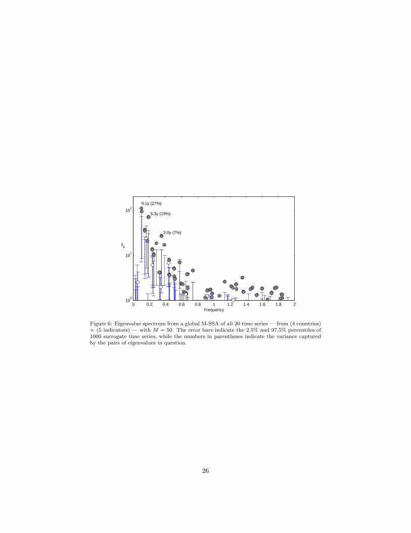
As was the case, at least in part, for the individual SSA analyses of subsetsof the three EU countries or five indicators in the two previous subsections(see again Tables 2 and 3), the eigenvalue spectrum in Fig. 6 clearly showsthree oscillatory pairs, each significant above the 95% level, with the previously

13

detected period lengths of approximately 9, 5, and 3 years. The sum of thevariances captured by these three pairs is 27 + 19 + 7 = 53% of the variance inthe total data set of the five indicators times the four countries, including nowthe U.S.

The longest period of 9 years is just barely significant at the 95% level,confirming the finding that this oscillation is hard to detect in the single timeseries (Table 1). It is especially the short overlap in time span, from 1981 to2008, in this global M-SSA analysis that complicates the distinction betweenrandom fluctuations and deterministic oscillations at this period length.

On the other hand, the 5- and 3-year oscillations can be identified moreoften in the single-channel SSA and the corresponding eigenvalues in Fig. 6 risewell above the 95% level of significance. Hence, it is highly unlikely that theseoscillations can be attributed to random fluctuations, even in the barely threedecades of data available at this time.

Next, we reconstruct the temporal behavior that corresponds to these threeoscillatory pairs. The reconstruction with a few RCs allows a streamlined view ofthe rather complex behavior of multiple countries and their indicators. It thushelps separate common behavior from single shocks. As a consequence, thebehavior seen in Fig. 7 is indeed rather homogeneous across all four countriesand their five indicators .

It is quite remarkable that the U.S. economy reveals the most coherentwithin-country behavior over the whole interval of observation (Fig. 7(d)), andthat all its indicators behave quite similarly, in both amplitude and phase. Forthe three EU countries, the amplitude modulation in time is still fairly consistentfor each country separately, but the phases are more variable, from indicator toindicator for the same country as well as across countries.

The UK is fairly strongly linked to the U.S. during the ’90s (Fig. 7(a)), butit shows a more erratic behavior recently, probably due to its stronger Europeanintegration in the last two decades. On the other hand, The Netherlands andItaly are generally more closely linked over the entire data span, and theirmacroeconomic behavior is quite similar. In the ’90s, both countries clearly lagbehind the U.S. and the UK, while in recent times this delay has been reduced.

Finally, to quantify the participation of each country and of its indicators inthe three global oscillatory modes, we analyze the variance of the correspond-ing RCs for each time series separately (Fig. 8). The 9-yr oscillatory mode isstrongest in the European countries, where it clearly dominates consumption.In the U.S. market, the importance of this mode is clearly quite limited, exceptfor the exports. This match between EU consumption and U.S. exports pointsto an obvious link between the two markets.

The second oscillatory mode, with a period length of five years, has quitea different behavior from one country to another. In the case of the UK, thismode has nearly the same energy for all aggregates, whereas for the Netherlandsand Italy, the energy varies substantially from one indicator to another. Thisdifference is in particular interesting insofar as the U.S. economy is concerned,since the business cycle there is dominated by a 5-year oscillatory mode (Grothet al., 2012). In this context, Fig. 8 supports a closer connection of the UK as

14

a whole to the U.S. economy.For the Netherlands and Italy, the picture is more complex since both coun-

tries are known to be more strongly linked to the European market. The con-sumption, for example, in both these countries shows a much weaker contri-bution of the 5-year oscillations, although their stronger participation in theexports supports a link to the U.S. market.

The third pair, with a period length of three years, exhibits overall smallervariance, in agreement with the univariate SSA analyses. The picture for the3-year mode in Fig. 8 is less informative and we are not able to associate thismode either to any particular country or to a particular indicator. Other marketmechanisms that we have not taken into account in the present analysis mayplay a role and it would be certainly of interest to extend the analysis to severaladditional countries with sufficiently long macroeconomic records.

6. Summary and concluding remarks

In this paper, we have carried out a frequency- and time-domain analysisof macroeconomic fluctuations in three European countries, namely Italy, TheNetherlands, and the United Kingdom (UK). For each country, five fundamen-tal indicators of the real aggregate economy — GDP, consumption, fixed in-vestments, exports and imports — have been considered in order to describeseveral aspects of the economic behavior of these countries, separately as wellas together. Despite the peculiarities of each individual economy, the resultsobtained from both uni- and multivariate investigations by singular spectrumanalysis (SSA) suggest the presence of quite a homogeneous multi-cyclical be-havior among the countries and indicators.

We have demonstrated that multivariate SSA (M-SSA) clearly goes beyonda simple analysis of cross-correlations and offers the reconstruction of a robust“skeleton” of the underlying dynamics. In this context, M-SSA helps identifydifferent market mechanisms, with their distinct characteristic time scales, andreduce the complex behavior of the system to a few robust oscillatory modes.

Such modes have been attributed, in other contexts, to the existence ofweakly unstable periodic orbits in the system’s phase space (Ghil et al., 2002).Albeit unstable, this type of closed orbits, also called limit cycles in dynamicalsystems theory, influence the system’s behavior and play an important role inthe synchronization process between the irregular evolutions of several macroe-conomic indicators within a country and between the economies of several coun-tries. Hence, these orbits leave their imprint in the economic system’s trajecto-ries — i.e. in the observed time series of indicators — and it is of special interestto identify and reconstruct them for a set of different indicators and countries.

In the present work, we have identified three main oscillatory modes in themacroeconomic evolution of these three EU countries: (a) a low-frequency os-cillation of about 9 years, which is statistically significant at the 95% level onlyin some of the time series in our data sets; (b) a 5-year oscillation that is clearlydominant in all three countries; and (c) a 3-year oscillation, which shows less

15

energy and is especially present in Italy and The Netherlands. Our analysis hasfurther been extended to the U.S. economy and, in agreement with the findingsof Groth et al. (2012), the pervasive character of the 5-year oscillatory mode inthe EU countries we had analyzed could indeed be attributed to its prevalencein the U.S. economy.

Finally, the statistical results in this paper support the predictions madeby Hallegatte et al. (2008), using the simple non-equilibrium dynamic modelNEDyM, namely the presence of an endogenous business cycle with a period ofroughly 5–6 years. The model’s 5–6-year periodicity is shared by all the indi-cators examined here, and it is consistent with the mean business cycle periodfound by several authors (Zarnowitz, 1985; King and Watson, 1996; Kontolemis,1997).

This agreement between NEDyM and the time-series analyses here is quiteencouraging. Further detailed numerical calibration of NEDyM to the actualhistory of macroeconomic indicators of major economies is necessary, though,in order to consolidate our confidence in the model’s predictve power.

To conclude, M-SSA provides a self-consistent and robust way of analyzingspatio-temporal behavior across countries and economic aggregates, where spaceis understood here in the sense of the phase space of the aggregates. This con-clusion is especially in line with the U.S. National Bureau of Economic Research(NBER) understanding of business cycles, namely that a recession is a signifi-cant decline in economic activity spread across the economy, i.e. not one thatis limited to GDP alone. In a multivariate framework, we have shown that theinclusion of more and more time series into M-SSA gives consistent results andhelps extract oscillatory modes that are shared across different economies.

In future work, it is certainly of interest to extend the present analyses toseveral additional countries with sufficiently long aggregate records. Doing sowould enable one to study shared mechanisms and synchronization effects on aglobal market.

7. Acknowledgments

We would like to thank Profs. Pietro Terna and Vittorio Valli for theirvaluable guidance to the two lead authors and for their many suggestions aboutthe economic interpretation of this work’s results. AG has received supportfrom the Groupement d’Interet Scientifique (GIS) Reseau de Recherche sur leDeveloppement Soutenable (R2DS) of the Region Ile-de-France.

16

Aadland, D., 2005. Detrending time-aggregated data. Economic Letters 89, 287–93.

A’Hearn, B., Woitek, U., 2001. More international evidence on the historicalproperties of business cycles. Journal of Monetary Economics 47, 321–46.

Allen, M., Robertson, A., 1996. Distinguishing modulated oscillations fromcoloured noise in multivariate datasets. Climate Dynamics 12, 775–784.

Allen, M. R., Smith, L. A., 1996. Monte Carlo SSA: detecting irregular oscilla-tions in the presence of colored noise. Journal of Climate 9, 3373–3404.

Atesoglu, H. S., Vilasuso, J., 1999. A band spectral analysis of exports andeconomic growth in the United States. Review of International Economics 7,140–152.

Baxter, M., King, R. G., 1999. Measuring business cycles: approximate band-pass filters for economic time series. Review of Economics and Statistics 81,575–593.

Baxter, M., Kouparitsas, M. A., 2005. Determinants of business cycle movement:a robust analysis. Journal of Monetary Economics 52, 113–57.

Blackman, R. B., Tukey, J. W., 1958. The measurement of power spectra fromthe point of view of communication engineering. Dover Publications.

Blanchard, O. J., Watson, M. W., 1987. Are business cycles all alike? Tech.rep., NBER Working Papers Series.

Broomhead, D. S., King, G., 1986a. Extracting qualitative dynamics from ex-perimental data. Physica D 20, 217–36.

Broomhead, D. S., King, G. P., 1986b. On the qualitative analysis of experi-mental dynamical systems. In: Sarkar, S. (Ed.), Nonlinear Phenomena andChaos. Adam Hilger, Bristol, England, pp. 113–144.

Calderon, C., Chong, A., Stein, E., 2007. Trade intensity and business cycle syn-chronization: Are developing countries any different? Journal of InternationalEconomics 71 (1), 2–21.

Chiarella, C., Flaschel, P., Franke, R., 2005. Foundations for a disequilibriumtheory of the business cycle: qualitative analysis and quantitative assessment.Cambridge University Press.

Coe, D., Helpman, E., 1995. International R&D spillovers. European EconomicReview 39 (7), 859–87.

Crivellini, A., Gallegati, M., Gallegati, M., Palestrini, A., 2007. Output fluctu-ations in G7 countries: a time-scale decomposition analysis. In: Mazzi, G. L.,Savio, G. (Eds.), Growth and Cycle in the Eurozone. Basingstoke, Hampshire,UK: Palgrave MacMillan, pp. 45–59.

17

Croux, C., Forni, M., Reichlin, L., 2001. A measure of comovement for economicvariables: theory and empirics. Review of Economics and Statistics 83 (2),232–41.

De Haan, J., Inklaar, R., Jong-A-Pin, R., 2008. Will business cycles in the Euroarea converge? A critical survey of empirical research. Journal of EconomicSurveys 22 (2), 234–273.

De Haan, J., Inklaar, R., Sleijpen, O., 2002. Have business cycles become moresynchronized? Journal of Common Market Studies 40 (1), 23–42.

Den Haan, W. J., Sumner, S., 2001. The comovement between real activity andprices in the G7. Working Paper 8195, NBER.

Dickerson, A., Gibson, H., Tsakalotos, E., 1998. Business cycle correspondencein the European Union. Empirica 25 (1), 51–77.

Esping-Andersen, G., 1999. Social Foundations of Postindustrial Economies.Oxford University.

Feenstra, R. C., Lipsey, R. E., Deng, H., Ma, A. C., Mo, H., 2005. World tradeflows: 1962-2000. Working paper 11040, NBER.

Frankel, J. A., Rose, A. K., 1998. The endogeneity of the optimum currencyarea criteria. Economic Journal 25, 1009–25.

Ghil, M., Allen, M. R., Dettinger, M. D., Ide, K., Kondrashov, D., Mann,M. E., Robertson, A. W., Saunders, A., Tian, Y., Varadi, F., Yiou, P., 2002.Advanced spectral methods for climatic time series. Reviews of Geophysics40 (1), 1–41.

Ghil, M., Vautard, R., 1991. Interdecadal oscillations and the warming trend inglobal temperature time series. Nature 350, 324–27.

Granger, C., 1969. Investigating causal relations by econometric models andcross-spectral methods 37 (3), 424–438.

Granger, C., Hatanaka, M., 1964. Spectral Analysis of Economic Time Series.No. 1. Princeton Stud, mathl Econ.

Granger, C. W., 1966. The typical spectral shape of an economic variable.Econometrica 34 (1), 150–161.

Groth, A., Ghil, M., Hallegatte, S., Dumas, P., 2012. The role of oscillatorymodes in U.S. business cycles. Working Paper 26, Fondazione Eni EnricoMattei (FEEM).

Gruben, W., Koo, J., Millis, 2002. How much does international trade affectbusiness cycles synchronization? Working Paper 0203, Federal Reserve Bankof Dallas.

18

Hallegatte, S., Ghil, M., Dumas, P., Hourcade, J., 2008. Business cycles, bifur-cations and chaos in neo-classical model with investment dynamics. Journalof Economic Behaviour and Organization 67, 57–77.

Higo, M., Nakada, S. K., 1998. How can we extract a fundamental trend froman economic time-series? Monetary and Economic Studies 16 (2), 61–111.

Hodrick, R. J., Prescott, E. C., 1997. Postwar U.S. business cycles: An empiricalinvestigation. Journal of Money, Credit and Banking 29 (1), 1–16.

Iacobucci, A., 2003. Spectral analysis for economic time series. Working Pa-pers 07, OFCE.

Imbs, J., 2004. Trade, finance, specialization, and synchronization. Review ofEconomics and Statistics 86 (3), 723–734.

Inklaar, R., De Haan, J., 2001. Is there really a european business cycle? acomment. Oxford Economic Review 53, 215–220.

Juglar, C., 1862. Des crises commerciales et de leur retour periodique, en France,en Angleterre et aux Etats Unis.

Kalemli-Ozcan, S., Sørensen, B., Yosha, O., 2001. Economic integration, in-dustrial specialization, and the asymmetry of macroeconomic fluctuations.Journal of International Economics 55 (1), 107–137.

King, R., Rebelo, S., 2000. Resuscitating real business cycles. Working Paper7534, NBER.

King, R., Watson, M., 1996. Money, prices, interest rates and the businesscycles. Review of Economics and Statistics 78, 35–53.

Kontolemis, Z., 1997. Does growth vary over the business cycle? Some evidencefrom the G7 countries. Economica 64, 441–60.

Krugman, P., 1993. Lessons of Massachusetts for EMU. New York: CambridgeUniversity Press, Ch. Lessons of Massachusetts for EMU, pp. 41–61.

Kydland, F. E., Prescott, E. C., 1982. Time to build and aggregate fluctuations.Econometrica 50 (6), 1345–1370.

Lisi, F., Medio, A., 1997. Is a random walk the best exchange rate predictor?International Journal of Forecasting 13, 255–67.

Long, Jr., J. B., Plosser, C., 1983. Real business cycles. The Journal of PoliticalEconomy 91 (1), 39–69.

Mane, R., 1981. On the dimension of the compact invariant sets of certain non-linear maps. In: Dynamical Systems and Turbulence. Vol. 898 of LectureNotes in Mathematics. Springer, Berlin, pp. 230–242.

19

Maravall, A., 2005. An application of the TRAMO-SEATS automatic procedure;direct versus indirect adjustment. Working Paper 0524, Bank of Spain.

Mazzi, G., Savio, G. (Eds.), 2006. Growth and Cycle in the Euro-Zone. PalgraveMcMillan.

Otto, G., Voss, G., Willard, L., of Australia, R. B., of Australia. EconomicResearch Dept, R. B., 2001. Understanding OECD output correlations. Eco-nomic Research Dept., Reserve Bank of Australia.

Penland, C., 1989. Random forcing and forecasting using principal oscillationpattern analysis. Monthly Weather Review 117, 2165–2185.

Solow, R., 1956. A contribution to the theory of economic growth. The QuarterlyJournal of Economics 70, 6594.

Stanca, L. M., 1999. Are business cycles all alike? evidence from long-runinternational data. Applied Economics Letters 6, 765–69.

Stock, J. H., Watson, M. W., 2002. Has the business cycle changed and why?Macroeconomic Annual, NBER.

Stock, J. H., Watson, M. W., 2005. Understanding changes in internationalbusiness cycle dynamics. Journal of the European Economic Association 3 (5),966–1006.

Takens, F., 1981. Detecting strange attractors in turbulence. In: DynamicalSystems and Turbulence. Vol. 898 of Lecture Notes in Mathematics. Springer,Berlin, pp. 366–381.

Vautard, R., Ghil, M., 1989. Singular spectrum analysis in nonlinear dynamics,with applications to paleoclimatic time series. Physica D 35, 395–424.

Vautard, R., Yiou, P., Ghil, M., 1992. Singular-spectrum analysis: a toolkit forshort, noisy chaotic signals. Physica 58, 95–126.

Von Storch, H., 1995. Inconsistencies at the interface between climate researchand climate impact studies. Meteorologische Zeitschrift 4, 72–80.

Woitek, U., 1996. The G7-countries: A multivariate description of business cyclestylized facts. In: Barnett, W., Gandolfo, G., Hillinger, C. (Eds.), DynamicDisequilibrium Modelling: Theory and Applications. Cambridge: CambridgeUniversity Press., pp. 283–309.

Zarnowitz, V., 1985. Recent work on business cycles in historical perspective:a review of theories and evidence. Journal of Economic Literature 23 (2),523–80.

20

1.5

2.5

3.5

4.5x 10

5

GDP

1

2

3

4x 10

5

CONSUMPTIONS

2

4

6

8

x 104

FIXED INVESTMENTS

4

8

12

x 104

EXPORTS

1955 1965 1975 1985 1995 2005

4

8

12

16x 10

4

IMPORTSUKThe NetherlandsItaly

Figure 1: Time series of gross domestic product (GDP), consumption, fixed investments,exports and imports for the United Kingdom (UK, blue curve), The Netherlands (green curve),and Italy (red curve). These raw series are based on EUROSTAT data and expressed inconstant, year-2000 Euros. See text and http://epp.eurostat.ec.europa.eu/ for details.

21

−2.5

0

2.5GDP

−2.5

0

2.5CONSUMPTION

−2.5

0

2.5 FIXED INVESTMENTS

−2.5

0

2.5

EXPORTS

1955 1965 1975 1985 1995 2005−2.5

0

2.5IMPORTS

Figure 2: Same time series as in Fig. 1, but pre-processed to extract the trend and normalizethe residuals so obtained. The underlying cyclical structure is visually apparent, and it is thesubject of the following analysis. Same color convention as in Fig. 1 and in subsequent figures.

22

0 0.5 1 1.5 2

107

108

109

1010

frequency [cycle/year]

Pow

er s

pect

rum

− R

aw G

DP

a)

0 0.5 1 1.5 2

10−2

10−1

100

101

102

frequency [cycle/year]Pow

er s

pect

rum

− D

etre

nded

GD

P, n

orm

aliz

ed &

sta

ndar

dize

d

9 y5 y

3 y

b)

Figure 3: Power spectral density (PSD) estimate for the GDP of the UK. Panel (a) PSDestimate for the raw data; panel (b) PSD estimate for the pre-processed trend residuals. PSDestimation was carried out by the Blackman-Tuckey algorithm with a Hanning window ofM = 100 quarters (Blackman and Tukey, 1958).

23

Figure 4: SSA analysis of the UK GDP: Monte Carlo singular spectrum of the transformedresidual series with M = 50. The filled circles represent the eigenvalues, while the lower andupper ticks of the error bars represent the 2.5% and 97.5% red noise percentiles.

24

1955 1960 1965 1970 1975 1980 1985 1990 1995 2000 2005−4

−2

0

2

4 Italy

−4

−3

−2

−1

0 UK

−4

−3

−2

−1

0 The Netherlands

Figure 5: SSA reconstruction of the 5-year oscillation in the GDP time series of the threecountries under study (solid line). This oscillation is represented by the first two eigenpairs ineach series, and it captures 39% of the total variance for the UK, 44% for The Netherlands,and 40% for Italy. The window widths are M = 50, 45, and 34 quarters, respectively. Thedotted curve in each panel is the same as the corresponding one in the first panel of Fig. 2.

25

0 0.2 0.4 0.6 0.8 1 1.2 1.4 1.6 1.8 210

0

101

102

Frequency

λk

9.1y (27%)

5.3y (19%)

3.0y (7%)

Figure 6: Eigenvalue spectrum from a global M-SSA of all 20 time series — from (4 countries)× (5 indicators) — with M = 50. The error bars indicate the 2.5% and 97.5% percentiles of1000 surrogate time series, while the numbers in parentheses indicate the variance capturedby the pairs of eigenvalues in question.

26

−0.06

−0.04

−0.02

0

0.02

0.04

0.06a) UK

−0.06

−0.04

−0.02

0

0.02

0.04

0.06b) The Netherlands

−0.06

−0.04

−0.02

0

0.02

0.04

0.06c) Italy

1985 1990 1995 2000 2005

−0.06

−0.04

−0.02

0

0.02

0.04

0.06d) U.S.

GDP Consumption Investments Exports Imports

Figure 7: Further results of the global M-SSA analysis in Fig. 6 — reconstructed behavior ofthe 20 indicators, grouped by countries, using RCs 1–2, 3–4, and 7–8, which belong to thethree significant oscillatory pairs of period length 9, 5, and 3 years, respectively. (a) The UK,(b) The Netherlands, (c) Italy, and (d) the U.S.; indicators for each country identified by thefive colors shown in the legend of panel (a).

27

0

0.005

0.01

0.015NL gdp

NL cons

NL fix inv

NL exp

NL imp

0

0.005

0.01

0.015IT gdp

IT cons

IT finv

IT exp

IT imp

0

0.005

0.01

0.015UK gdp

UK cons

UK finv

UK exp

UK imp

0 0.2 0.40

0.005

0.01

0.015US gdp

Frequency in cycles/year

ST

D

0 0.2 0.4

US cons

0 0.2 0.4

US inv

0 0.2 0.4

US exp

0 0.2 0.4

US imp

Figure 8: Standard deviation of the RCs as a measure of participation strength. The plotshows the RCs that correspond to the highly significant oscillatory pairs — namely RCs 1-2,3-4, and 7-8 — vs. their dominant frequency.

28