1 value and worth Introducing concepts of - Wiley-Blackwell · Introducing concepts of 1 value and...

Introducing concepts of value and worth1

1.1 Real estate: an introduction to the economic concepts

Within this book the concepts of worth, price and value are explored in terms of their chang-ing application to real estate markets. Underpinning all of these concepts is the theory of market economics. Whilst this book is not a text on land economics, it is important to introduce the principles upon which the relevant market practices have developed.

Under neoclassical economic theory, the three factors that contribute to economicwealth are normally taken to be:

• people

• money

• land.

Each factor is a resource that is deemed to be scarce and hence has value both to the indi-vidual and to society, and the study of economics is concerned with the allocation of theuse of that resource. Within the UK there is a mixed economy, in that resource allocationdecisions are taken partly by government on the basis of need, and partly by private individuals and corporate bodies on the basis of economic demand. Where real estate allocation decisions are based on need (for example, the provision of public goods and services such as hospitals and schools), these decisions are, as a broad-brush rule, taken onthe basis of least cost and value for money. Where the allocation decisions are based ondemand (for example, the provision of shops, offices for corporate use and private leisurefacilities), this is on the basis of economic demand, as expressed through the supply anddemand pricing model.

Under this paradigm, price is the product of the interaction of supply and demand.Given any level of demand and any given supply, price will adjust to produce an equilib-rium point at which the amount in supply matches the quantum of demand. If the demandfor a good falls and supply remains constant, price will also fall until it triggers people forwhom price was previously a barrier to enter the market. Conversely, if demand rises thenprice will rise too. However, over time – which is sometimes referred to as the fourth

Aims of the chapter

• To provide a context for the book.

• To distinguish it from others in thefield.

• To introduce the concepts of value,worth and price in the context of the

main players within the real estatefield.

• To provide an historical context for thethemes of the book.

REA_C01.qxd 22/3/06 2:33 PM

2 Real estate appraisal

dimension of economics – there will be an adjustment in supply and/or demand inresponse to price change.

The assumptions on which the pricing model is deemed to work are that:

• there are a multiplicity of separate economic actors, so that no one individual caninfluence the operation of the market;

• there is homogeneity of product;

• all participants are both rational and perfectly informed;

• there are no barriers to entering and exiting the market; and

• the market can make immediate marginal adjustments to accommodate change.

This is of course a very simplified explanation, and it does not relate easily to the real estate market. Whilst the normal market relationship is for supply and demand to be in equilibrium, in certain circumstances the property market may suffer disequilibriumwhere turnover effectively ceases and no clearing price exists. Disequilibrium wasobserved in the property crash of 1973.

Real estate lies within both the public and the private realm, and any decisions regardingits use allocation (and hence pricing) are affected by government intervention in the formof taxation and land use controls. Real estate is also a unique commodity in that its supplyis fixed in overall terms, though not in relation to its specific use. It is also unique in thateach unit of land or building is individual, in terms of location if nothing else, and it istherefore said to be a heterogeneous product.

Real estate is also unusual in that the motivation for ownership may be for utility pur-poses (for example, the requirement for a factory as a production unit or a shop as an outletfor manufactured goods) or for investment (that is, as a means of receiving a prospectiveincome and capital return on a capital outlay). A further complexity of real estate as a sub-ject for economic analysis is the nature of the land conversion process, whereby land is adevelopable commodity to which value can often be added by the carrying out of a schemeof building works, or a change in the effective use of the land or/and the buildings upon it.This development process is constrained both by the nature and extent of demand and bypossible and actual physical, legal, financial, political and planning restrictions.

In the light of the above, it is not surprising that the land markets have given rise to acomplex set of models and theories as they seek to deal with the effects of legislation andthe lack of perfect knowledge that interfere with the ‘pure’ operation of the market mech-anism (for a fuller explanation see, for example, Ball et al., 1998; Eccles et al., 1999;Warren, 2000; Harvey and Jowsey, 2003).

In summary, the economics of land and real estate markets is particularly complex due to:

• The relatively fixed nature of land: whilst fixed in physical terms, the availability ofland for use will alter depending on land use planning regulations; it is therefore capableof change over time.

• A lack of transparency and published data: one of the key features of the property markets is their lack of transparency. Unlike equities markets, there is no free and easilyaccessible source of information on transaction prices. Whilst this situation is changingrapidly with the development of web-based services and the opening of the LandRegistry to enquirers, data may not be free. Within institutional property markets,

REA_C01.qxd 22/3/06 2:33 PM

Introducing concepts of value and worth 3

greater transparency has been afforded by the setting up of the Investment PropertyDatabank (IPD) which for the past 20 years has monitored the movement of yields andrents in respect of values of many institutional owner assets, but it is neither completenor capable of disaggregation at the local or individual asset level, except to the contributing property owner, although it is freely available at aggregated level.

• The nature of legal interests: unlike other assets, property can be held in many waysand, strictly speaking within the UK, it is not held outright as all title is vested in theCrown. In legal terms, the owner holds an ‘interest’ in land. This can be freehold (fulllegal rights to deal with the asset as the owner wishes subject only to planning and otherstatutory restrictions); leasehold (the owner has an interest in the asset for a fixed termonly and on terms that are set by a legal relationship between the freeholder and thelessee); or – following the passing of the Leasehold Reform and Commonhold Act 2002 – commonhold, whereby a joint ownership may be achieved. Currently there is little analysis of the likely effects of commonhold, given its recent introduction in 2004.

• Heterogeneity: the nature of the commercial property markets is that each property willbe different; not only is the location unique, but properties also tend to differ in size,shape, specification and amenities. This leads to difficulty in comparing one withanother and hence in achieving consistency within any pricing model.

• The motivation of ownership: as stated above, real estate may be owned as a resource within which to carry out economic or social activity or as an investment.Fundamentally, it is the ability to provide utility that drives the economic worth of theasset. The demand for land is a derived demand; it relates to the surplus that can beachieved through its usage. If there is no possibility of real utility being achieved thenthere will be no occupational demand and hence no value.

To the investor, however, it is not the utility of the asset that matters directly but thesecurity of income flow that can be achieved through rent. Investors are also concernednot just with cash flow security but with capital security and the prospects for both thecash flow and capital growth. Against this they will balance the risks of default and the attractiveness and likely returns available through investment in other asset classes,such as equities and bonds.

In summary, the role of property within the economy is observed to be important as aresource to the business and social community. However, it also has a second role withinthe economy as a home for investment funds, for both domestic and overseas investors.Where an individual or company, institution or government has spare capital not requiredfor immediate consumption, it can either be held as a cash investment or invested in a capital asset. In the main capital markets the options open to investors range from govern-ment stock, to equities, to property, to derivatives relating to these markets.

Historically, many property text books have focused on property valuations andappraisals from the perspective of institutional investors. In the late 1970s average institutional property weightings were over 20% of investment assets. By 2000 this figurehad fallen to below 5%, but it recovered by 2004 to just under 8%.

However, the proportion of the property market owned by institutions is only a small partof the whole commercial property market. In Chapter 9 it is shown that UK corporates andthe UK Government own an estimated £486 billion of property assets. In Chapter 10 the

REA_C01.qxd 22/3/06 2:33 PM


gross property assets of public and private property companies are estimated at £210 billion.In contrast, institutional property holdings are estimated at around £100 billion.

Institutional property investment has an important role to play in the workings of thecommercial property market, but in practice the corporate, government and property company ownership is some seven times greater. The latter plays a major role in the workings of the property market and thus deserves detailed consideration. In consequence,any major rise or fall in demand for investment property or property that is capable ofbeing valued using the investment method will have an affect on the wider economy.

1.2 Aims of the book

There are many books that provide a comprehensive cover of the subject of real estate eco-nomics and others that deal specifically with the pricing of property. Many of these coverin-depth issues within the field of investment valuation (see, for example, Baum andCrosby, 1995b); others concentrate overall on valuation as a technical discipline from the viewpoint of the consultant valuer (Davies et al., 2000; Rees and Hayward, 2000). The aim of this book is not to revisit that which is already very adequately covered else-where, although inevitably there is a significant amount of overlap. Instead it discussesaspects of practice and theory that link the world of investment valuation with that of the owner-occupier.

It is the authors’ contention that for too long the debate that has informed practice hasconcentrated on the needs of the institutional investment owner of real estate, almost to theexclusion of those of the occupier. Yet without an occupier ready and willing to take alease, now or in the future, a property investment has little real worth.

This focus of approach on the institutional landlord has been understandable, and in part is a result of the dramatic growth of funds under investment from the mid 1970s to the early 1980s. However, property as a home for investment funds has a relatively shorthistory, dating back only 30 to 40 years in the UK and a far shorter time in most other EU countries (see, for example, Dubben and Sayce, 1991; Ross Goobey, 1992; Fraser,1993; Scott, 1996). Institutional investment in property grew in an environment whereplanning restrictions on the supply of new, developed property encouraged occupiers totake long lease terms (normally 25 years) with periodic upward only rent reviews and full tenant liability for the physical asset (McIntosh and Sykes, 1985).

These so-called institutional leases were influential in that they enabled the incomestream from property to be viewed in much the same way as other financial assets in thecapital markets. This stimulated a body of research-based books including those byMacLeary and Nanthakumaran (1988); Brown (1991); Baum and Crosby (1995a) andBrown and Matysiak (2000). All these aimed at exploring ways of applying equity-market-based financial appraisal techniques to property investment analysis. The fun-damental economic paradigm on which all these works have been based is that of neoclassicism; hence the works have striven to pursue rational quantitative approaches to the pricing conundrum.

In recent years, however, changes have been discernable and the spotlight has movedacross to occupiers and owner-occupiers. This book concentrates on the following themesin particular:

REA_C01.qxd 22/3/06 2:33 PM


• The growth in the influence of the corporate occupier as related to a breakdown of insti-tutional leasing patterns, and the growth in finance leases rather than operational leases.

• The growth of new models of finance that influence property decision-making.

• The increasing recognition of the simplistic nature of maximising the ‘single bottomline’ – that is, the economic return – and the rise of the sustainability agenda.

Our aim in this book is to begin to address these issues in relation to the financial appraisalof property for both investors and corporate occupiers, and to relate this at all times to thepractice implications.

1.3 New influences on the real estate market

1.3.1 The role of property and its growth as a managed asset

Land, in its improved or unimproved state, is fundamental to most human activity. It alsohas enormous implications for commercial activity as the resource base within which most commerce takes place. Some years ago the London Business School calculated that commercial property alone was worth half the value of the companies traded on the stockmarket and over double the value of Government stock (Currie and Scott, 1991). But in presenting these findings, the authors were explicit as to the difficulties they had indeveloping a methodology for capitalising the value of the UK’s corporate estate, as theyhad been unable to find any publicly available statistics. Even an examination of companyaccounts did not give a full and clear picture, as is explained later in this book.

Setting aside the issue of how property capital values in the balance sheet are calculated,the implication of the Currie and Scott report was that property requires strategic managementto ensure that its use aligns to business objectives (Edwards and Ellison, 2003). However, asuccession of research reports, from Avis et al. (1989) to Bootle and Kalyan (2002), have con-cluded that many businesses are underutilising and undermanaging their property assets.

The reasons for this observed underuse and undermanagement are many and com-plex. In part they relate to historical factors, and in part to the way assets are held on thebalance sheet. However, they also relate to the failure, until recently, of many owners tomeasure the economic performance of their assets, in terms of either their return on cap-ital employed or their added value to the business. This scenario is changing rapidly, andthrough this book a number of the issues of performance measurement that are funda-mental to providing corporate owners with a deeper understanding of the performance of their real estate are explored.

As owners take a more analytical approach to their asset management, so it will beexpected that the type and specification of the properties they require to occupy will alsoalter. Already there is evidence that occupiers are seeking to intensify their use of officeproperties by changing the space requirements and moving to new ways of working suchas ‘hot desking’ and ‘hotelling’. More radically, some activities, previously located in theUK are being outsourced to other countries (for example, call centres to India). Thesechanges will affect the future aggregate levels of demand for property and, in addition,affect the location, specification and longevity of property. This will in turn influence theattractiveness of property as an asset and its price in the marketplace.

REA_C01.qxd 22/3/06 2:33 PM


Another change explored in the book is that taking place in the structure of leases. Formany years long leases were the norm; this is now breaking down, with companiesdemanding either freeholds or very long leases for their core occupational needs, and shortflexible leases for their ancillary activities. Nowhere has this trend been more prevalentthan in the office market, with average lease lengths a third of those prevailing in the early1990s. The reasons for the shortening of lease patterns are complex but relate in part tochanges in the accounting regulations in relation to the treatment of leaseholds on the balance sheet; in part they are a reflection of the needs of occupiers to be more dynamic inresponse to the changing business environment.

The shortening of lease patterns has had two discernible effects. First, it has begun toaddress the lack of separation between the property occupational and investment mar-kets that has been a hallmark of both practice and the literature. Second, and of more consequence for this book, it has required the development of appraisal techniques thatcan accommodate more flexible and less predictable income flows and that can be appliedto unravel comparable rental evidence of transactions where, for example, rent review patterns, rent-free periods or capital inducements are different. This has led to the growthof applications of discounted cash flow techniques, as explored in subsequent chapters.

1.3.2 The new financial paradigms

Investors in real estate are making a choice to allocate a proportion of their funds to property in preference to other asset classes. In doing so they will apply a series of fin-ancial analysis techniques to assist in their decision-making. It is therefore important thatproperty appraisers and analysts have a grasp of these models in order that they can advise appropriately. However, appraisers in the real estate industry can be criticised forhaving in the past been slow to embrace new theories and methodologies.

One of the key debates within the real estate appraisal field in recent years has been theissue of whether properties should be appraised by comparison with other transactions(valuation) or by reference to their prospective cash flows using discounted cash flow (DCF)techniques. Proponents of DCF argue for its greater ability to compare property performanceand deal with non-standard cash flows – key requirements in a market that is moving towardsmore flexible cash flows. In this book the DCF approach is both explained and promoted asa methodology that should be used alongside traditional valuation techniques.

Another issue related to appraisal techniques concerns the relationship between realestate and the financial markets. Whilst much of the research work from the competingequities and bonds markets in the finance literature is ground-breaking and potentiallyinteresting, analysts recognise that real estate has fundamentally different characteristicsfrom equities and bonds; this poses questions as to how far the theories from these marketsare valid for and can be applied to the real estate market.

Within the real estate field, as will be detailed in later chapters, appraisal techniques thatdeal with assets in a portfolio context relate in the main to the conventional finance the-ories developed between the 1960s and 1980s. Under these theories, there has been anassumption that investment decision-making is driven by rational economic behaviourand that investors have sought always to maximise returns and minimise risk. Modernportfolio theory, developed by Markowitz (1959) and subsequently extended by others

REA_C01.qxd 22/3/06 2:33 PM


such as Sharpe, Lintner and Mossen, adopted the rational assumption. Furthermore, theseauthors worked on the basis that markets are ‘efficient’, that is, that prices fully reflect allrelevant financial data (see, for example, Fama and Miller, 1972). Since the mid 1980s,and some twenty years after these theories began to be applied in the financial field, property analysts have sought to use them for real estate.

In the meantime, just as these ‘modern’ finance theories have begun to gain groundwithin the real estate field, new theories have emerged which relax the assumptions ofrationality and efficiency. New finance models accept the reality of inefficient markets and adopt a range of techniques from econometrics to arbitrage (Chen et al., 1986) andbehavioural models (Tversky and Kahneman, 1981) to explain investor behaviour. Thesenew developments are explored in order to illustrate how far they can be used within theproperty asset allocation process.

1.3.3 The rise of the sustainability agenda

The above sets out the conventional economic view as related to property. Whilst this stillprovides the framework within which the markets operate, it is coming under increasingchallenge from what is called the ‘fourth factor’. Lovins et al. (1998) and Hawken et al.(1999) argue that the industrial and service economies, which our current economic theories seek to analyse and which at present form the basis of economic decision-making,are flawed. This is, they argue, because they fail to integrate the basic resources of air,water and ecological balance within the economic value sets; instead they treat them asfree goods, with the consequence that the natural capital essential to supporting our eco-nomic activity is being depleted at a fast and unsustainable rate.

Hawken et al. (1999) contend that industrial (and post-industrial) societies will need to adjust their decision and resource allocation models to include natural capital within the economic equation. In this they concur with the ‘factor four’ principle (Lovins et al.,1998) that economic survival rests on resource productivity growing fourfold to enableeconomic life to be sustained into the future.

The notion of balancing the desire for economic development with society’s ambitionfor sustainability in both social and environmental terms has gained very rapid groundsince the so-called Brundtland definition of sustainability was published in 1987 (WCED,1987). This definition, namely that sustainable development meets the needs of todaywithout compromising the ability of future generations to meet their own needs, has beenthe subject of much debate. However, the concept has been increasingly enshrined withinsupranational and national legislation and policy. Within the UK, the first sustainabledevelopment strategy was produced by government in 1994, following the Rio EarthSummit’s call in 1992 for all countries to produce such a strategy.

The Rio Summit laid out eight principles of sustainability, which can be summarised asfollows:

• The fundamental right of all human beings to an environment that is adequate for theirheath and well-being.

• The conservation and proper use of the environment (including the built environment)in a way that benefits both current and future generations.

REA_C01.qxd 22/3/06 2:33 PM


• The promotion of bio-diversity to ensure ecosystem maintenance.

• The monitoring of environmental standards and the publication of data related thereto.

• The prior assessment of the environmental impacts of significant developments.

• That all individuals are informed of planned activities and given rights to justice.

• That conservation is integral to the planning and implementation of development activities.

• That states should co-operate towards mutual implementation.

Underlying these principles are three themes:

• The promotion of environmental well-being, so that environmental degradation is min-imised and natural resources are used to the greatest benefit. This implies inter alia:

° conservation of non-renewable energy resources;

° reduction of greenhouse gas emissions;

° promotion of use of renewable energy sources; and

° management of resources, including waste management.

• The protection of, and proper respect for, people so that the common human conditionis improved, as measured by indices such as the United Nations Human DevelopmentIndex. This implies progress towards:

° improvements in working conditions;

° adequate care of the less advantaged;

° social legislation to ensure good governance at all levels; and

° appropriate educational and employment opportunities in terms of education andwork.

• The creation of an economic context in which social and environmental goals can beachieved. Whilst Hawken et al. (1999) are optimistic about the prospects for this, othersare less so.

The implications of the rise of the sustainability agenda may seem on first view to bedivorced from the issue of real estate pricing. This may have been the case some years ago,but now both environmental concerns and social well-being are beginning to influence theoperation of the property markets and the pricing of property assets.

First, there is a rapidly emerging raft of social and environmental legislation that affectsreal estate directly (see, for example, the Planning and Compulsory Purchase Act 2004;the 2005 England and Wales Building Regulations and the Disability Discrimination Act1995). The advent of more energy controls and the proposed introduction of energy labelsfor buildings are other examples of ways in which occupiers will be affected by the growthof concern for sustainability. In addition, social responsibility policies are now to be foundwithin many corporate organisations (see, for example, Henry, 1999). Collectively, thesefactors will affect the levels of property pricing in the marketplace in the future, if they donot do so already (St Lawrence, 2003).

The impact of the sustainability agenda will also have an effect on the attitudes ofinvestors in property and hence the prices that they are willing to pay. In the wider invest-ment field, the establishment of the Dow Jones Sustainability Index in the US and of theFTSE4Good in the UK have demonstrated high comparative performances by companieswith a strong commitment to corporate social responsibility. In turn this has attractedinvestment funds to such companies. A further driver is to be found in the requirement,

REA_C01.qxd 22/3/06 2:33 PM


since 2000, for pension funds to have social responsibility policies. This has led to many ofthe major funds and other institutional investors seeking ways to implement such policiesin their investment practice, including their property investment practice (Sayce andEllison, 2003). A survey by Parnell and Sayce (1999) found little evidence of pricingbeing directly affected at that time, but respondents were very strong in their opinion thatin the future these matters would be significant.

In summary, whilst the established supply and demand model of pricing continues, therise of worldwide concerns about sustainability matters is likely to act as an increasingconstraint on models and to influence the behaviour of all players in the economy, includ-ing property occupiers and investors.

1.4 Structure of the book

This book is structured to take readers through the key decision points within the propertyinvestment process, whether that investment is for rental and capital return or forms part ofthe corporate asset base. Before doing so, this chapter introduces the main techniques thatare conventionally used by valuers and appraisers in determining the market value of aproperty asset. These techniques are not developed in any detail here, as this material iscovered in many other books (for example, Isaac and Steley, 2000; Johnson et al., 2000)and aspects of the methods are developed in later chapters. The focus in the book is onexploring the new market practices that are evolving in response to the shifting investmentand corporate agenda, and these relate to worth. Whilst accepting that a dictionary mayregard the words ‘value’ and ‘worth’ as synonymous, to the property appraiser they arenot. Accordingly, this chapter introduces the notion of worth to provide a context for the subsequent analyses.

Chapter 2 deals with the property purchase decision in some detail by exploring the factors that influence this decision, both for investors and for corporate occupiers. The purchase process that is required of the consultant valuer is then explained.

Investors will wish to place their decision within the context of the entire investmentspectrum of opportunities to ensure that they are purchasing an appropriate asset at anacceptable price; hence Chapter 3 considers the appraisal of property within the context ofthe multi-asset portfolio and Chapters 4, 5 and 6 explore the calculation of market value.Whilst the approaches adopted in these three chapters do not introduce any concepts that are radically different from those espoused by the established literature, they are considered from a professional practitioner’s perspective, and some of the newer con-straints in relation to the emerging corporate social responsibility agenda are introduced.

Price will be a major consideration for the purchaser of any property. However, moreimportant than the market price is what an asset is worth to a prospective purchaser and,following purchase, an analysis of this continued value to the organisation is required.These aspects are developed in Chapter 7 where the calculation of worth to the individualis considered.

To the property owner, risk is also a major concern. There are two aspects to this: risk asit relates to the pricing of an individual asset, and risk in relation to the interaction of thatasset with others in the portfolio. The ways in which each can be analysed and built intopricing models are detailed and discussed in Chapters 8 and 12, respectively.

REA_C01.qxd 22/3/06 2:33 PM


The point that property values are ultimately dependent upon occupational demand has already been made. We have indicated that we are concerned with property investorsand occupational ownership. Chapter 9 analyses some of the influences on occupationaldemand and considers in detail the buy or lease decision, whilst Chapter 10 explores someof the property funding and financing decision issues.

Once a property sits within either an occupational or an investment portfolio, its contribution to economic return should be measured and its future likely contribution tothe portfolio estimated. Accordingly, Chapter 11 and Chapter 13 consider the measure-ment of return and forecasting, respectively.

One of our objectives in writing this book has been to minimise the number of mathe-matical equations used; however, no study of property pricing can avoid these altogether,and some mathematical examples have been included. Appendix A contains details of theformulae that have been used within the book and, to further assist readers, Appendix Bcontains details of a web site from which further detailed and updated examples that illu-strate the techniques and principles put forward in the book can be downloaded for use.

1.5 Worth v. price v. value: definitions

This book is concerned with the concepts of worth and value and their relationship to price within the real estate markets. The differences between them and their relevance in practice are developed further in Chapter 7. In this chapter, the background and underlyingdistinctions are introduced.

The concepts of worth and value and their relationship to price are fundamental issueswithin the operation and regulation of real estate markets. If a dictionary is consulted, thewords worth, price and value are normally found to be described as synonymous or to havedefinitions that are at least in part interchangeable. Additionally, in other countries theremay be little or no distinction made between these words (for a discussion of this see Adairet al., 1996). There may be significant differences in practice: for example, in the UK valuations are undertaken by a valuer and an appraisal is undertaken by an appraiser/property investment surveyor advising the purchaser or employed by the purchaser, whilstin the US an appraiser undertakes both valuations and investment appraisals. However, inthe UK in recent years, the distinction in meaning between worth, price and value hasbecome an important matter in defining the activity of the real estate professional.

Until the 1990s, most professionals operating in real estate would have used the wordsprice, worth and value interchangeably. A debate was then triggered, primarily by therapidly changing market conditions of the late 1980s and early 1990s. During this periodvaluations prepared primarily for bank lending purposes came under the scrutiny of thecourts as a succession of valuers were called to account for their valuations which (withthe benefit of hindsight) had proved to be over optimistic. The professional response wasto examine, amongst other things, the regulations under which valuers operated, and toclarify the terminology used by them. The Royal Institution of Chartered Surveyors(RICS) set up the Mallinson Committee, headed by Michael Mallinson, the then chief surveyor to Prudential Property Investment Managers.

From the publication in 1994 of the Mallinson Report (Mallinson, 1994) to the publica-tion in 2003 of the overhauled RICS Appraisal and Valuation Standards (RICS, 2003)

REA_C01.qxd 22/3/06 2:33 PM


there was a lively debate. In the early 1990s the emphasis on valuation accuracy in the UK was intense (Drivers Jonas, 1991; Lizieri and Venmore-Rowland, 1991, 1993;Matysiak and Venmore-Rowland, 1995; Matysiak and Wang, 1995; McAllister, 1995 and Brown and Matysiak, 2000) and debate focused on the need for the consultant valuer/appraiser to be in tune with the needs of the client, an issue raised by Mallinson.However, following Mallinson the focus of debate shifted from accuracy – though this remains an issue – to semantics. Mallinson was of the view that a number of differentbases of valuation were required and that a distinction should be drawn between value in exchange (market value) and value in use (worth). In response to this, RICS pro-duced two guides: one to commercial valuations (RICS, 1996) and the other on worth(RICS, 1997). Since that time the understanding of a differential between the terms hasdeveloped.

Whilst in the UK some consensus has begun to emerge, the question of the definition ofworth, price and value presents continuing problems in an international context (see, forexample, McParland et al., 2000). It is important to attempt to define the concepts beforeprogressing to appropriate valuation methodologies.

The word value can be used to describe different but related concepts in terms of realestate. It may be viewed as a general, all-encompassing term that incorporates the threemain types of value: price, market value and worth. The term valuation has specific pro-fessional definitions and for the UK is defined within the RICS Appraisal and ValuationStandards (RICS, 2003). Elsewhere, it is defined by both the European standards(TEGoVA, 2003) and the International Valuation Standards (IVSC, 2003). Although thewording differs in each case, the essence is that a valuation is an estimation of the mostlikely selling price on the open market, on the basis of both a willing seller and a willingbuyer. However, in practice, the valuation figure may not be the same as the price actuallyachieved. This may be due to imperfections within the property market or the presence of aspecial purchaser to whom the property may have a value over and above its worth to otherpotential buyers; or it may reflect a timing discrepancy, since valuations assume that theproperty marketing has already been undertaken and the transaction is due for completionas at the valuation date. In reality, the length of time it takes for the marketing of a propertyinvestment and agreement of a price can be several months, during which time marketmovement may occur that places the agreed price out of line with the then prevailing market values. Another problem that can lead to differences between the valuation and theprice achieved may relate to the lack of current comparable evidence on yields and rentsupon which to base the valuation. Price is derived from the interaction of supply anddemand, but the supply of land for specific uses is relatively fixed and is slow to adjust tochanges in demand, leading to price anomalies.

In the context of value, price and worth, Hoesli and MacGregor (2000) distinguishbetween four different concepts:

• Price is the actual observable money exchanged when a property investment is boughtor sold. In most other markets price is given, but in the property market every propertyinterest is different and requires an individual estimate of value to guide the buyer andseller in their negotiations to agree a price. Price can be fixed by negotiation, throughtender bids or at auction.

REA_C01.qxd 22/3/06 2:33 PM


• Value is therefore an estimation of the likely selling price. In other markets, wherehomogenous goods are sold, the price is not estimated but is determined from markettrading and is usually used to describe an assessment of worth.

• Individual worth is the true value to an individual investor using all the market information and available analytical tools and can be considered as the value in use.

• Market worth is the price a property investment would trade at in a competitive andefficient market using all market information and available analytical tools. A validmodel of calculation of market worth should reflect the underlying conditions of themarket at the time. This should therefore be distinguished from market value, whichaccepts a less than perfect knowledge of market information.

In practice in the UK property investment market, value and worth can currently be distinguished as follows:

• Value is obtained through the gathering and application of comparable evidence. Thecomparable evidence is gathered from transactions involving properties similar interms of effective rents (for more on this, please refer to Chapter 4), and yields. The valuation methods use rents and rental levels as at the valuation date, and yields inwhich risk and growth are implied (i.e. traditional valuation methods are used).

• Worth is frequently calculated using discounted cash flow methods and is considered in terms of whether or not a required or hurdle rate of return is achieved.

The debate on definitions is not confined to the UK; nor is there yet a settled position.The role of the International Valuation Standards Committee in devising and promotinginternationally recognised and accepted definitions and processes has become of increas-ing importance, with a significant majority of countries with established property marketsnow involved in the process of developing international definitions and standards. As timegoes by there will doubtless come a point at which full professional understanding isreached, but we have not arrived at it yet!

1.6 Conventional approaches to establishing value

In the UK, valuation practice has traditionally used five different methods. A summary ofthese is set out below. Four are commonly used for assets that are normally traded in themarketplace; the fifth relates to assets that are seldom if ever traded except as part of thesale of a company.

Before detailing the methods used, it must be stressed that the choice of method will depend upon the purpose for which the valuation is being prepared. The most common purpose is for market transaction; however, valuations are also commonlyrequired for loan security or for inclusion in company accounts. (Valuations are needed for other purposes as well, notably in relation to taxation, but these are not addressed inthis book.)

For more details on the five methods of valuation, please refer to Scarrett (1991) andDavies et al. (2000), and for their application to specific property types see Rees andHayward (2000).

REA_C01.qxd 22/3/06 2:33 PM


1.6.1 The comparative method

The comparative method is used where there are comparable transactions involving properties with characteristics similar to those of the property in question. For example, in the case of vacant possession residential property, the prices of similar three-bedroomhouses can be compared and used to determine the value of the three-bedroom property in question. The skill of the valuer is to make adjustments to reflect the differencesbetween the comparable properties and the property being valued.

This method is also used for the valuation of agricultural land, such that the value perhectare is derived from similar farm land that has been sold. Where zoning for new devel-opment is uniform, this method can be used as a valuation method for development land,on a square metre or hectare basis.

In commercial property transactions in the UK, this method is increasingly used as aninformative figure that can provide the valuer with background information relative to theproperty, such that the property being valued and the comparables being used are looked at in terms of the capital value per square metre of the gross or net usable floor area.However, the comparative method is unlikely to be used as a standalone valuation methodin the UK.

1.6.2 The investment method

The investment method is used to value income-producing vacant possession propertywith the potential to produce a rental income and owner-occupied commercial propertythat could be let to produce a rental income. In the UK the investment method is seen as themain method of valuing commercial property.

This method considers in today’s terms the net income streams that a property will produce currently and in the future. Using the present value of £1 methodology, each ofthese annual income streams is discounted to arrive at today’s value. As the current andprospective net income streams are determined as at the valuation date, the present valuemultipliers can be aggregated to produce years purchase multipliers (for example, yearspurchase in perpetuity, years purchase single rate or years purchase deferred for a setperiod). Further information on these valuation formulae is set out in Appendix A.

In the investment method there are five key inputs

• The passing rent.

• The estimated open market rental value as at the valuation date. This is determined fromcomparable evidence of recent lettings and relates to the effective open market rentalvalue and not the headline open market rental value. Please refer to Chapter 4 for moredetails on this.

• The valuation yield(s) are determined from comparable evidence of recent markettransactions, from which the years purchase multiplier is derived and applied to the net rents.

• The purchaser’s costs of undertaking the purchase transaction. Net valuation yields are calculated on the basis that the return to the investor includes the costs of the transaction.

REA_C01.qxd 22/3/06 2:33 PM


• The length of the void period and the associated costs before the vacant accommodationbecomes income-producing. These figures relating to voids are in many instancesimplied into the valuation yield: the valuation yield is adjusted in line with comparableevidence to reflect the impact of current or prospective voids. In practice, if the void orpotential void is material then it is likely to be included explicitly in the valuation.

It is worth noting that the underlying methodology used in the investment method ofvaluation utilises the concept of the time value of money, namely that £1 today is worthmore than £1 receivable in the future. The figure is a product of when the money isreceived and the discount rate used. This discounting methodology is the same as that usedin the discounted cash flow appraisal method (see section 1.7.1). However, in the invest-ment method of valuation it is the current levels of rents that are used, and future growth,risk and property-specific characteristics are implied within the valuation yield (the multi-plier). In contrast, the discounted cash flow appraisal method uses a target or required rateof return as the discount rate, but makes explicit assumptions as to what the future netrental cash flows will be.

1.6.3 The residual method

The residual method is used to value development sites and existing properties that havethe potential to be redeveloped. Additionally, where the land cost is known this methodcan be used to determine the developer’s profit.

The method involves many variables, and the value derived for the site can be very sensitive to relatively small changes in these variables. The traditional assumption is thatthe development and site purchase are financed using 100% borrowed money.

A straightforward way of considering how the residual method of valuation works is tolook at the time line of events in a development scheme (Fig. 1.1). The building costs andfees are rolled forward, together with the interest charges. To these are added the lettingand sale costs and the developer’s profit, to give the total development cost as at the datethe property is expected to become substantially let. At this date a deemed sale is assumed.The valuation of the completed and let property is carried out, usually using today’s rentallevels and net yields for comparable new properties. This figure is known as the grossdevelopment value, and from it is deducted the total development cost. The difference isthe value of the land as at the deemed sale date in the future. This future land valueincludes the interest cost of holding the land, and these interest costs are stripped out usingthe present value of £1 formula to produce the current value of the site/land.

When undertaking residual valuations, practical considerations come to the fore. Theseinclude the ability to gain the necessary planning consents and any likely conditionsattached thereto, the site conditions, the availability of building contract labour, the cost of

Letting anddeemed saleBuy site Start build Finish build

Fig. 1.1 The timeline of events in a development scheme.

REA_C01.qxd 22/3/06 2:33 PM


borrowings and the time likely to be required to complete the development. The simplicityof the residual method of valuation is both its strength and its weakness. To overcome itssimplicity and a number of the assumptions used, a detailed discounted cash flow appraisalcan be undertaken as well.

1.6.4 The profits method

The profits or accounts method is used where the occupier of commercial property uses the accommodation as an integral part of their business, such that the value is linked to the profitability of the business, and the level of profit expected determines the ability of the trader to pay for premises.

The method, which is normally regarded as specialist, is used primarily for the valuationof trading premises and is normally, though not always, restricted to types of propertiesthat change hands most frequently on a freehold basis. Examples of properties where theprofits method is used include hotels, public houses, petrol filling-stations and some leisureproperties. Yet where sufficient transactions and comparable evidence exist for similarproperties because of an increasing number of lettings, there is less reliance on thismethod. This is explored further in Chapter 4.

1.6.5 The cost approach

The cost approach to valuation is used when a property is occupied by an owner, but there is a real lack of comparable evidence of transactions for similar properties. In suchcases a cost basis of valuation is used; however, the resultant figure will be finalised by the client, with the valuer reporting the figure ‘subject to the ongoing profitability’ of thebusiness.

The underlying assumption for this method is that the property forms part of the assetsused in an ongoing business and as such, in an accountancy context, can be treated similarly to plant and machinery. The method is used within both the private and publicsectors so its use is not restricted to profit-orientated property (see, for example, Sayce andConnellan, 2000). In the case of public sector properties, the assumption is made as to thecontinuance of the service.

Because the method is only used in cases where there is a lack of market transaction evidence, it follows that it is not used for the purposes of open market sale; indeed, its usewithin the UK is restricted to book or company accounting and statutory purposes (forexample, taxation and compensation for compulsory acquisition). The same is not true insome other countries, such as the US, where it is used as a check against market value(Gelbtuch et al., 1997), and some European countries, particularly those that are emergenteconomies (Adair et al., 1996).

The cost approach to valuation assumes that the value to the owner relates to the cost ofreproducing the asset by rebuilding. The valuation comprises two elements: the land and the buildings. First the land is valued with due regard to comparables. At the time ofwriting (2005), the land will be valued in its existing use (see, for example, RICS, 2003;IVSC, 2003). However, changes to international accounting regulations mean that this assumption is set to change, and new guidance issued by IVSC in 2004 to ensure

REA_C01.qxd 22/3/06 2:33 PM


compliance with accounting standards introduces the concept of market value for the landelement (IVSC, 2004)

The building element is then valued to determine the depreciated replacement cost ofthe building. The calculation of the depreciated replacement cost (DRC) requires the estimating of the current replacement cost of the building, normally assuming a modernsubstitute building then depreciating this in relation to the future potential life of the actualbuilding. There is much debate as to how such depreciation should be conducted (see, for example, Britton et al., 1991; RICS, 2003), but most valuers adopt a straight lineapproach. The value of the property is the sum of the land value and the depreciatedreplacement cost.

Examples where this method is used include power stations, chemical plants, jetties andother specialised properties. It is worth remembering that the cost approach to valuation is akin to an accounting method of assessing the asset’s value to the business rather than its value to a third party or its open market value. For this reason, a valuation of this kindshould not normally be used as a basis for secured lending; neither does it give any indication as to the likely realisable price in the marketplace.

Please see Spreadsheet 1 for worked examples of each of the five valuation methods.

1.7 Additional approaches to appraisal

In addition to the five conventional methods of valuation, other methods are discernible inthe market place both in the UK and elsewhere. These are now introduced.

1.7.1 The discounted cash flow appraisal method

Absent from the above five methods of valuation is the discounted cash flow (DCF)appraisal method of valuation. In many countries, including the US, Australia and NewZealand and across Continental Europe, this DCF method of appraisal is used as a valuation method in its own right – effectively a sixth valuation method. Until recently in the UK, however, discounted cash flow (DCF) was considered to be an analytical tooland not a valuation method.

In the bond and equities markets, discounted cash flow is an established valuationmethodology. In contrast, in the UK real estate investment market DCF is generally seenas an investment appraisal tool. However, in a growing number of countries that haveestablished and sophisticated property investment markets (for example, the US andAustralia) the use of DCF methodologies has been extended such that they are recognisedas a valid valuation method. Increasingly this is also the case in the UK, for a number ofreasons which are set out below.

The techniques used in DCF appraisals are detailed in Chapter 3, but to present a contextfor the explanation of why they are being adopted, the basic terminology is explained here.

In essence a DCF requires the valuer or appraiser to arrive at an estimate of the actualanticipated cash flows over a specified time horizon, normally between 10 and 15 years.These cash flows will be the rent currently passing together with any uplifted rent

REA_C01.qxd 22/3/06 2:33 PM


anticipated during the period as a result of reviews and market movement. Accepting boththat cash flows in the future will be prone to risk and that there is a time value to money(see Chapter 3 for an explanation of interest rate theory), each cash flow in the future is discounted at a chosen rate of interest (known as the hurdle rate, the target rate or the investor’s required return). Cash flows beyond the specified time horizon are then capitalised using a single capitalisation rate and discounted at the hurdle rate. The resultantfigure is the estimated gross present value (GPV) of the asset. This represents the figure atwhich an investor with the specified required rate of return should be prepared to purchasethe investment. Where the purchase price and costs are included the figure becomes the netpresent value (NPV), and this is usually the figure that is sought.

Clearly, altering the required rate of return will alter the resultant figure; an increase inthe rate required will lower the NPV, and vice versa. For many investors it is useful toknow, for any proposed price, what rate of interest (or discount rate) would result in theinvestment being just worthwhile. It is possible, using simple spreadsheet methodology, tocalculate this rate, which is know as the internal rate of return (IRR).

Having described the nature of a DCF, it must be asked why this it set to becomeaccepted as a legitimate sixth method of valuation. As has already been explained, withinthe UK there has been a tradition of long leases but this is not paralleled in most othercountries. More commonly, leases are short, with structural repairing obligations being a landlord’s responsibility; there are no upward only rent reviews and in their place isindexation in line with, for example, a cost of living index (Adair et al., 1996). This results in major differences in the assessment of market value.

• The tendency is to use a simple investment approach or initial yield valuation, in whichthe passing rent is capitalised and any reversionary potential is simply incorporated into the capitalisation yield.

• Alongside the initial yield valuation method, DCF appraisal is used as a complementaryvaluation methodology.

In the UK, many factors are driving practitioners to consider the adoption of such anapproach. These drivers, described in more detail in subsequent chapters, include:

• Changes to lease terms, including shortening of the term and the prospect of possiblepolitical intervention relating to lease terms.

• Changes to accounting standards which require the inclusion of property at ‘fair value’.

• Changes to stamp duty on leases, which is a powerful driver towards shorter occupa-tional leases.

As leases change in response to these market drivers, so too must valuation techniques.Before consideration is given to the application of DCF analysis techniques as a method ofdetermining whether or not a property is fairly valued, DCF methodology will be exam-ined briefly to demonstrate how it can be used as an explicit valuation technique.

In the US, DCF is used as a valuation method, such that IRRs for different properties (inparticular shopping centres) can be quoted as comparables. In the UK, the use of DCF as avaluation tool operates in a slightly different manner. Unlike normal DCF analysis, whichlumps together all the cash flows to produce a net cash flow which is then analysed, UK DCFvaluation methodology often splits the anticipated cash flows into four main tranches:

REA_C01.qxd 22/3/06 2:33 PM


• Bond tranche number 1: this relates to the rental income passing for the term of thelease, and excludes any potential uplifts. It is valued as if it were a government bond,with the discount rate reflecting the creditworthiness of each tenant.

• Bond tranche number 2: this relates to the difference between the rent passing and thecurrent market rental value of the property. This income stream is deemed to be morerisky than tranche number 1. It is valued as if it were a bond, with the discount ratereflecting the creditworthiness of each tenant, plus a margin to reflect the uncertainty ofthe increase actually being achieved at the next rent review.

• Equity tranche number 1: this relates to the expected increases in the rents receivable overand above the current passing rents and the estimated market rental value. These potentialincome streams are discounted at a relatively high discount rate to reflect their riskiness.

• Equity tranche number 2: this relates to the ‘exit value’ of the property at the end of theDCF analysis period. Again, an equity-type discount rate is used to reflect the risks ofobsolescence, depreciation and poor market performance.

For buildings let on long leases to high-quality tenants, this explicit DCF valuationmethod can produce values higher than the traditional open market valuation methods, dueto the current positive yield gap between bonds and property yields. In contrast, where theoccupational leases are short the values can come in significantly lower. It is not surprisingthat this methodology is used internally by a number of life insurance companies whoview commercial property as a substitute for bonds and a method of providing for theirannuity contracts. However, the variance in end results from those achieved through conventional methods has resulted in considerable resistance amongst some members ofthe valuer community. Nonetheless, the move towards its adoption is gaining momentumand the RICS standards (RICS, 2003) now contain specific reference to DCF methodologyfor calculating investment worth.

Whilst DCF is gaining acceptance as a method to be used as complementary to estab-lished techniques, it is worth noting that in the US valuation practice dictates that a seriesof valuations should be undertaken by the appraiser: namely, that each of the six methodsof valuation should be undertaken (subject to applicability), and the valuer should producea valuation in the context of prevailing local market conditions and the figures producedunder the various methods. In practice the investment method (also known in the US as the direct capitalisation method), in conjunction with the discounted cash flow appraisalmethod, are the main methods relied upon for commercial property investments.

Discounted cash flow as an appraisal method is considered in more detail in Chapter 3and subsequent chapters.

1.7.2 Statutory valuations

There is a strong case for including a seventh valuation method, as it is used by Germanopen end funds who are major players in the European property investment market. Where they exist as a genuine valuation method, statutory valuations should be added tothe list.

In the UK such methods do not exist in the property investment market. They relate onlyto cases of taxation and compensation. However, in Germany, financial institutions

REA_C01.qxd 22/3/06 2:33 PM


(which include German open end funds) in particular are required by law to value property investments under the terms set out in statutes. In this context, the WertV.(Wertermittlungsverordnung) provides a detailed code of valuation concepts, which areused by practising valuers. The details of such valuation methods are outside the scope ofthis book, and for further information readers are referred to Adair et al. (1996). However,when such valuation methods are used it is important to compare the valuation figure withthe market value. The statutory valuation method can frequently produce a significantlyhigher figure, and this should be acknowledged.

1.8 An introduction to the drivers for DCF

Until recently, there was a clear distinction between the use of traditional valuations andDCF appraisal techniques. This distinction has become blurred, such that DCF appraisaltechniques are used as both a valuation and an appraisal technique, and this blurring isbeing accelerated by the shortening in occupational leases taken by tenants.

The forces for change in the UK property market that will impact on and shorten leaselength are as follows:

• Changes to stamp duty in the 2004 Finance Act make the amount of tax charged a function of the lease length: the longer the lease, the greater the tax burden payable bythe lessee. This has prompted a demand for shorter leases.

• Changes to the UK and International Accounting Standards coming through in 2005will change the way in which occupational leases are shown in company accounts.Currently, occupational leases are not shown in the balance sheet, but under the newrules they will be shown as both an asset and a liability. This will raise the gearing levelsof retail and hotel companies significantly.

• There is government pressure for shorter, flexible leases. In 2002 the Labour Govern-ment told the property industry that, unless it saw landlords offering more flexible leaseterms to tenants, it would bring forward legislation. In particular, upward only rentreviews are seen as being too onerous for tenants, given the cyclical nature of propertymarkets.

In other countries where short leases are common, tenants usually have the ability toquit at either three- or five-yearly intervals. In short leases, the lease terms tend to be different from those seen in the traditional 15 to 25 year UK lease, as shown in Table 1.1.

Table 1.1 Typical lease terms.

UK leases

Full repairing

• Tenant responsible for structural repairs

Upward only rent reviews

Break clauses not very frequent

• Security of income linked to tenant quality

Rental cash flows relatively predictable

EU and US leases

Internal repairing

• Landlord responsible for structural repairs

In EU a link to indexation common

Break options frequent

• Void risk potential at breaks

Rental cash flows relatively unpredictable

REA_C01.qxd 22/3/06 2:33 PM


The style of lease contract influences the valuation methodology used. Where there areshort leases, the tendency is for valuers to use different valuation methodologies fromthose used in the UK, where there is the benefit of long leases (Table 1.2). Thus in the EUand US, DCF is used alongside the initial yield method as a valuation method. It there-fore seems reasonable to conclude that, as UK leases get shorter, UK lease terms will start to change and will move into line with those seen in countries where short leases are common.

A shift in the UK to shorter leases is thus likely to have a knock-on effect in terms of thevaluation methods used. If the UK follows the US and EU experience, there will be a moveto the use of initial yield-based valuations and a growth in the use of DCF techniques byvaluers.

There is another driver for change in the way that property is valued. This is the increas-ing use by the investor of combined equity (the investor’s own money) and debt finance(typically money borrowed from a bank). This move is in part to strive for increasedreturns, and also to enlarge the pot of money available to increase the portfolio size andreduce the exposure to specific risks. These issues are considered in more detail inChapters 9 and 12, respectively.

The incorporation of debt into the property transaction renders traditional valuationsonly partially useful. Whilst valuations are required by the lender in order to satisfy a num-ber of their lending ratios – for example, initial and exit loan to value ratios – traditionalvaluations do not help in defining the prospective net cash flow profile of the investment,which is required by the bank to determine their debt service cover and interest coverratios. Furthermore, traditional valuations do not provide figures relating to prospectivegeared (equity) returns.

Thus a move to shorter leases and a growing use of debt finance is prompting a growinguse of DCF methodologies alongside traditional valuations. This widening of valuationmethodologies will require the UK valuation profession to become accustomed to usingDCF techniques. From the authors’ experience, DCF is a methodology of which many UK property professionals have little practical experience. In Chapter 3 there is an introduction to property appraisal and investment analysis techniques, which discusseshow DCFs can be structured and the key inputs and outputs.

Table 1.2 Valuation methodologies.

UK

Investment method as outlined above

DCF rarely used as a valuation methodology but commonly used as a tool of analysis of worth

EU and US

Initial yield method predominantly used

• Void risk and income changesincorporated implicitly into the yield

• UK-based investment methodseldom used

DCF often used alongside the initialyield method as a second view on thevalue

REA_C01.qxd 22/3/06 2:33 PM


1.9 SummaryThis chapter has sought to introduce the main themes that run through the book. Realestate is a key element within the economy; it therefore requires to be appropriately managed and this in turn requires reliable and accurate appraisals to be carried out. In particular, as the established economic paradigms are increasingly challenged by the rise of the sustainability agenda, so there will be a need for a response among property professionals. There is also a need both to better understand the role of property as an operational asset and investment medium and to relate its appraisal more closely to themethodologies used in other markets.

The role of the adviser has traditionally been that of advising on market value or likelyprice in the marketplace. In subsequent chapters we argue that this role now requires theacquisition of new skills within the field of appraisal.

Currently, property pricing is achieved using one or more of five valuation methods.These have been in place for many years and are generally well understood. However,where properties are being held as investments, the traditional methodology is increas-ingly under challenge by the sixth method in the adviser’s armoury, namely discountedcash flow (DCF). The increasing use of DCF as an appraisal method in addition to valuation methods provides a key theme for this book. DCF is used within the investmentand occupier market, and is widely used in risk and portfolio analysis.

The issue of risk is also critical to appraisal and we devote two chapters to its considera-tion. However, any consideration of property appraisal should not be done without dueconsideration of the operational needs that underpin demand, and a chapter is devoted tooccupier considerations. These are addressed in other chapters too.

In presenting this book we have sought to balance the theories that underpin practicewith the applications, and readers are advised to consult the web link provided inAppendix B to gain new and updated information on applications.

ReferencesAdair, A., Downie, M.L., McGreal, S. and Vos, G. (1996) European Valuation Practice: Theory and

Techniques. London: E&FN Spon.Avis, M., Gibson, V. and Watts, J. (1989) Managing Operational Property Assets. Reading:

University of Reading.Ball, M., Lizieri, C. and MacGregor, B. (1998) The Economics of Commercial Property Markets.

London: Routledge.Baum, A. and Crosby, N. (1995a) Property Investment Appraisal, 2nd edn. London: Routledge.Baum, A. and Crosby, N. (1995b) Over-rented properties: bond or equity? A case study of market

value, investment worth and actual price. Journal of Property Investment & Finance, 13 (2): 31– 40.

Bootle, R. and Kalyan, S. (2002) Property in Business – A Waste of Space. London: RICS.Britton, W., Connellan, O. and Crofts, M. (1991) The Cost Approach to Valuation. London: RICS.Brown, G. (1991) Property Investment and the Capital Markets. London: Chapman Hall.Brown, G. and Matysiak, G. (2000) Real Estate Investment: A Capital Markets Approach. London:

FT Prentice Hall.Chen, N.-F., Roll, R. and Ross, S. (1986) Economic forces and the stock market. Journal of

Business, 59 (3): 383–403.

REA_C01.qxd 22/3/06 2:33 PM


Currie, D. and Scott, A. (1991) The Place of Commercial Property in the UK Economy. London:London Business School.

Davies, K., Johnson, T. and Shapiro, E. (2000) Modern Methods of Valuation. London: EstatesGazette Ltd.

Disability Discrimination Act 1995. www.legislation.hmso.gov.ukDrivers Jonas (1991) The Variance in Valuations. London: Drivers Jonas.Dubben, N. and Sayce, S. (1991) Property Portfolio Management. Routledge: London.Eccles, E., Sayce, S. and Smith, J. (1999) Property and Construction Economics. London:

International Thomson.Edwards, V. and Ellison, L. (2003) Corporate Property Management: Aligning Real Estate with

Business Strategy. Oxford: Blackwell Science.Fama, E. and Miller, M.H. (1972) The Theory of Finance. New York: Holt, Rhinehart, and Winston.Fraser, W.D. (1993) Principles of Property Investment and Pricing, 2nd edn. Basingstoke:

Macmillan.Gelbtuch, H., Mackmin, D. and Milgrim, M. (1997) Real Estate Valuation in Global Markets.

Illinois: The Appraisal Institute.Harvey, E. and Jowsey, J. (2003) Urban Land Economics. Basingstoke: Palgrave Macmillan.Hawken, P., Lovins, A. and Lovins, L. (1999) Natural Capitalism: Creating the Next Industrial

Revolution. Boston: Little, Brown and Co.Henry, E. (1999) The value of environmental performance to financial stakeholders. UNEP Industry

and Environment, Jan–Mar: 11.Hoesli, M. and MacGregor, B. (2000) Property Investment: Principles and Practice of Portfolio

Management. Harlow: Longman.Isaac, D. and Steley, T. (2000) Property Valuation Techniques. Basingstoke: Palgrave Macmillan.International Valuations Standards Committee (2003) International Valuation Standards 2003.

London: IVSC.International Valuations Standards Committee (2004) International Valuation Standards 2004.

London: IVSC.Johnson, T.A., Davie, K. and Shapiro, E. (2000) Modern Methods of Valuation of Land, Houses and

Buildings, 9th edn. London: Estates Gazette.Lizieri, C. and Venmore-Rowland, P. (1991) Valuation accuracy: a contribution to the debate.

Journal of Property Research, 8: 115–122.Lizieri, C. and Venmore-Rowland, P. (1993) Valuations, prices and the market: a rejoinder. Journal

of Property Research, 10: 77.Lovins, L., Von Weizsäcker, E. and Lovins, A. (1998) Factor Four: Doubling Wealth, Halving

Resource Use. London: Earthscan.MacLeary, A. and Nanthakumaran, N. (eds) (1988) Property Investment Theory. London: E&FN

Spon.Mallinson, M. (1994) Commercial Property Valuations: The Report of the Mallinson Committee.

London: RICS.Markowitz, H. (1959) Portfolio Selection: Efficient Diversification of Investments. New York: John

Wiley & Sons.Matysiak, G. and Venmore-Rowland, P. (1995) Appraising Commercial Property Performance

Rankings. Paper to the RICS Cutting Edge Conference, Aberdeen University, September 1995.Matysiak, G. and Wang, P. (1995) Commercial property market prices and valuations: analyzing the

correspondence. Journal of Property Research, 12: 181.McAllister, P. (1995) Valuation accuracy: a contribution to the debate. Journal of Property

Research, 12: 203.

REA_C01.qxd 22/3/06 2:33 PM


McIntosh, A.P.J. and Sykes, S.C. (1985) A Guide to Institutional Property Investment. London:Macmillan.

McParland, C., McGreal, S. and Adair, A. (2000) Concepts of price, value and worth in the UnitedKingdom – towards a European perspective. Journal of Property Invesmentment & Finance, 18 (1): 84–102.

Parnell, P. and Sayce, S. (1999) Investment Attitudes towards Green Buildings. London: DriversJonas/Kingston University.

Planning and Compulsory Purchase Act (2004) www.legislation.hmso.gov.ukRees, W. and Hayward, W.H. (eds) (2000) Valuations: Principles into Practice. London: Estates

Gazette Ltd.Ross Goobey, A. (1992) Bricks and Mortals: Dream of the 80s and Nightmare of the 90s – Inside

Story of the Property World, London: Random House Business Books.Royal Institution of Chartered Surveyors (1996) Commercial Property Valuations: An Information

Paper. London: RICS.Royal Institution of Chartered Surveyors (1997) The Calculation of Worth: An Information Paper.

London: RICS.Royal Institution of Chartered Surveyors (2003) Appraisal and Valuation Standards. London:

RICS.Sayce, S. and Connellan, O. (2000) The Valuation of Non-Profit Oriented Leisure Property.

London: RICS Research Foundation.Sayce, S. and Ellison, L. (2003) Integrating sustainability into the appraisal of property worth:

identifying appropriate indicators of sustainability. American Real Estate and Urban EconomicsAssociation Conference, RICS Foundation Sustainable Development Session, Skye, Scotland,21–23 August 2003.

Scarrett, D. (1991) Property Valuation: The Five Methods, London: E&FN Spon.Scott, P. (1996) The Property Masters. London: E&FN Spon.St Lawrence, S. (2003) Review of the UK Corporate Real Estate Market with regard to availability

of environmentally and socially responsible office buildings. Paper for Cambridge Programme forIndustry Sustainability Learning Network, 2003.

TEGoVA (2003) European Valuation Standards (the ‘Blue Book’). London: TEGoVA.Tversky, A. and Kahneman, D. (1981) The framing of decisions and the psychology of choice.

Journal of Science, 211 (4481): 453–458.Warren, M. (2000) Economic Analysis for Property. London: Architectural Press.World Commission on Environment and Development (1987) Our Common Future. Oxford:

Oxford University Press.

REA_C01.qxd 22/3/06 2:33 PM

Forecasting13

13.1 Introduction

Whenever investment or operational property purchase decisions are made, some sort offorecast will be used either explicitly or implicitly. In many cases this will be an intuitiveforecast based on purchasers’ experiences of past trends which they project into the future.In the case of the operational owner the forecast will inevitably concentrate on the abilityof the property to meet business requirements, but it should nevertheless also include reference to future property markets. For the investor, however, the need to forecast likely future changes in property market conditions and, in particular, the ability of the individual property to perform in the future will be of great significance in the decision-making process.

Over the past 20 years the availability of data to investors on property markets hasimproved enormously. This has notably been through the medium of IPD (InvestmentProperty Databank) who produce short- and long-run data on 90% of institutionally owned assets. The increased flow of reliably sourced data, combined with an increasingavailability of computer-based statistical software, has enabled investors to access and apply statistical techniques. It is now possible to undertake relatively sophisticatedmodelling techniques in respect of market movements, rental levels and yields, to producebetter cross-media comparison in ways that were previously unavailable. The questionremains as to whether these techniques do and will enable investors to improve theirrisk/return profiles. In this chapter the various techniques now available and increasinglyin use are explored. First, however, it is necessary both to define a forecast and to distinguish it from an appraisal.

Aims of the chapter

• To detail the nature and aims of forecasting and place these within the context of property investment andmanagement.

• To distinguish between a forecast andan appraisal.

• To provide an overview of currentpractices and techniques used withinthe real estate industry for undertakingforecasts.

• To describe methods of establishingtrends, including the examination ofsources of data and their reliability.

• To explain regression analysis in itsvarious forms (simple, multi-variate,linear and non-linear).

• To discuss the relevance of propertycycles in forecasting techniques, and the use of barometers and leadindicators.

REA_C13.qxd 22/3/06 2:30 PM Page 297


13.2 Forecasting and appraisals

Investing in property usually implies a long-time commitment. The average holdingperiod for property held within the IPD annual property index is estimated at around seven years. Therefore both owners and investors need to satisfy themselves that their purchase appraisals are founded in well-based forecasts of the future. However, a fore-cast is not the same as an appraisal; the latter projects cash flows into the future but uses market assumptions, whereas a forecast encompasses the use of many different techniques.

In a discounted cash flow framework the future expected values for these variables can be determined at one end of the spectrum by practitioner/professional judgement and at the other by forecasts derived from sophisticated models. In practice a combinationof the two is often used. Put simply, an appraisal is an investor’s view of the worth of an investment property. In this appraisal there are a number of assumptions relating to thefuture. These assumptions or variables drive the projected performance of the investmentand that in turn provides the estimate of worth of the asset to the investor or corporateoccupier.

The nature of an appraisal has been defined in earlier chapters and it is important here todistinguish between an appraisal and a forecast. In essence an appraisal will provide theinvestor or owner-occupier with an estimated net present value (NPV) of the property at agiven date based on primarily market-derived evidence and using a discount rate that isconsidered appropriate to the class of property, including any specific and market risk factors. The market data used will relate to current and projected rental values and yields,including estimates of rates of likely depreciation. As with all discounted cash flow analyses, the analysis period will be set; this will frequently be between 5 and 15 years. At the end of the cash flow period an ‘exit’ value will be taken and this will relate to projections of the most likely market conditions.

In preparing an appraisal, estimates must be made. In establishing these inputs to thecalculations some quantitative forecasts may have been undertaken or commissioned.However, the appraisal itself is not a forecast of future value: it is the interpretation of a range of data that will enable the investor or owner to form a view as to whether the market is currently under- or over-pricing the asset. In the event that those operating and advising in the market are fully aware of the same forecast materials as the appraiser,convergence between market value and appraisal may result. So, in summary, a forecastcan inform the appraisal but an appraisal is not a forecast, nor is it necessarily dependent on one.

13.3 Aims of forecasting

The aim of any forecast is to provide a ‘best estimate’ of the future in relation to specificelements of likely change. Essentially, therefore, its purpose is threefold:

• To highlight where there are opportunities for future successful activity.

• To pinpoint areas of risk.

• By quantification, to inform decision-making both at the point of purchase and subsequently.

REA_C13.qxd 22/3/06 2:30 PM Page 298

Forecasting 299

Within a property context, forecasting can be used to:

• Detect market level trends that may effect either whole portfolios or sectors within the portfolio, either positively or negatively.

• Predict future rental growth or yield patterns by analysing likely movements in theirunderlying ‘drivers’.

• Establish projected financial performance.

It is in the nature of all forecasting that it is an essentially inaccurate activity. There-fore care must be taken in assessing the confidence that can be placed in any forecast. For this reason, as detailed below, forecasts are frequently considered in probability terms.

Whilst every property appraisal and valuation has a perception of the future built withinit, this has in the past normally been predicated on experience and intuition. Increasingly,investors are now seeking quantitative approaches to assist them with their decision-making. This will be of importance especially at times when either economic uncertaintyprevails or the property market is weak and data hard to establish. The RICS recognisesthis within its appraisal standards (RICS, 2003: GN5) but only deals with the issue in verygeneral terms.

Within a management context, forecasting details such as levels of future rent may be critical in the hold/sell decision.

13.4 Methods of forecasting

13.4.1 Time series

Many forecasts involve the use of time series analysis. A time series is an orderedsequence of values for a variable taken at equally spaced points through time. Forecastingtime series movements can be approached from two different basic angles:

• Identifying historic patterns in the time series and self-projecting the series into thefuture (trend analysis).

• Identifying relationships between variables and the market, and using those variables to project the movement of the market into the future (regression analysis).

This chapter identifies and introduces the self-projecting methods of forecasting, butfocuses on regression analysis. Regression analysis is the basis of most commerciallyavailable forecasts of the property market so knowledge of how to construct a model is beneficial when interpreting and using the results. Detailed time series analysis andeconometrics as a discipline are considered to be outside the scope of this book; coverageis restricted only to topics that are likely to be useful for the property professional.

13.4.2 Decomposition analysis

Decomposition analysis is based on the premise that time series are composed of a numberof elements or components, normally defined as seasonal, trend/cycle plus a random orirregular variation.

REA_C13.qxd 22/3/06 2:30 PM Page 299


If these components are assumed to be independent of each other, then the time series isthe sum of the components. If they are assumed to be interrelated, then a multiplicativeapproach is used.

Once the values of each component have been determined, they can be recomposed by addition or multiplication to project them forward and create a forecast. Software packages such as SPSS (Statistical Package for Social Scientists) have built-in proceduresthat can isolate these components and provide forecasts using, for example, de-trended orde-seasonalised data.

13.4.3 Forecasting using smoothing analysis

Time series data is expected to exhibit some form of random variation through time.Additionally, it may exhibit an underlying cyclical, trend or seasonal component. To identify these components, smoothing analysis can be used to remove unwanted variationand project the time series forward.

• Moving average models self-project the time series into the future by averaging pastperiods and projecting that view forward. The optimal number of periods to averagewill need to be found by trial and error, although some statistical packages may do thisautomatically. Basically, the assumption used is that the average of values at the end of the series is the best estimate of the current mean value around which the data isfluctuating.

• Exponential smoothing works in a similar way to the moving average model, exceptthat the model assigns exponentially decreasing weights to past observations, so morerecent observations have more impact on the forecast.

Whichever approach to time series is taken, the underlying principle is the same: the view of the future is found by an analysis of past transactions and context. Whilst thevarious types of time series analysis develop different ways of dealing with abnormalitiesand variation, there is an underlying assumption that the past is a good guide to likelyfuture performance. If that underlying assumption is ill-founded, so too is the forecast.

13.5 Forecasting using linear regression models

Linear regression analysis is used to examine the relationship between one dependent variable and one or more independent variables. The results from the analysis can then be used to forecast the dependent variable using known values of the independent variableor variables.

The following sections examine the steps involved in building forecasting models using regression. However, each step needs to be considered within the constraints of the following five assumptions which will become clearer further into the chapter:

• The dependent variable is a linear function of the independent variables plus an errorterm.

• The error terms sum to zero.

• The errors at each point are random from the previous error and show no trend.

REA_C13.qxd 22/3/06 2:30 PM Page 300

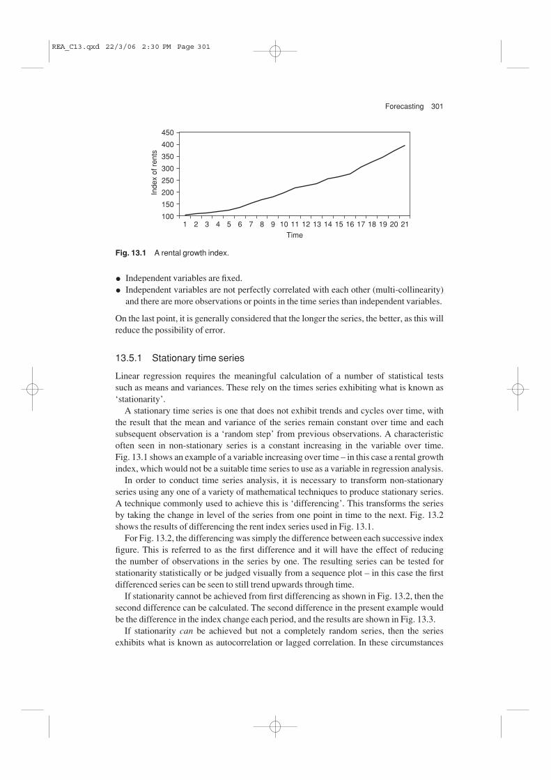
Forecasting 301

• Independent variables are fixed.

• Independent variables are not perfectly correlated with each other (multi-collinearity)and there are more observations or points in the time series than independent variables.

On the last point, it is generally considered that the longer the series, the better, as this willreduce the possibility of error.

13.5.1 Stationary time series

Linear regression requires the meaningful calculation of a number of statistical tests such as means and variances. These rely on the times series exhibiting what is known as‘stationarity’.

A stationary time series is one that does not exhibit trends and cycles over time, with the result that the mean and variance of the series remain constant over time and each subsequent observation is a ‘random step’ from previous observations. A characteristicoften seen in non-stationary series is a constant increasing in the variable over time. Fig. 13.1 shows an example of a variable increasing over time – in this case a rental growthindex, which would not be a suitable time series to use as a variable in regression analysis.

In order to conduct time series analysis, it is necessary to transform non-stationaryseries using any one of a variety of mathematical techniques to produce stationary series.A technique commonly used to achieve this is ‘differencing’. This transforms the series by taking the change in level of the series from one point in time to the next. Fig. 13.2shows the results of differencing the rent index series used in Fig. 13.1.

For Fig. 13.2, the differencing was simply the difference between each successive indexfigure. This is referred to as the first difference and it will have the effect of reducing the number of observations in the series by one. The resulting series can be tested for stationarity statistically or be judged visually from a sequence plot – in this case the firstdifferenced series can be seen to still trend upwards through time.

If stationarity cannot be achieved from first differencing as shown in Fig. 13.2, then thesecond difference can be calculated. The second difference in the present example wouldbe the difference in the index change each period, and the results are shown in Fig. 13.3.

If stationarity can be achieved but not a completely random series, then the seriesexhibits what is known as autocorrelation or lagged correlation. In these circumstances

450

400

350

300

250

200

150

1001 2 3 4 5 6 7 98 10 11 12 13 1514 2116 17 18 19 20

Time

Inde

x of

ren

ts

Fig. 13.1 A rental growth index.

REA_C13.qxd 22/3/06 2:30 PM Page 301


a moving average, autoregressive model or combination of both models may be moreappropriate. One example of such a model is the autoregressive integrated moving average(ARIMA) model.

Given that the time series used in Figs 13.1–13.3 is an index of rental growth, it wouldbe more appropriate to take the first difference as the percentage change between points in the index instead of subtracting one index figure from another. When compared to Fig. 13.2, the percentage change shown in Fig. 13.4 eliminates the trend or drift; the seriesfluctuates around a mean point with no distinct cycle. Simply subtracting index numbersas in Fig. 13.2 does not allow for the effect of compounding in the series, hence it has adefinite trend.

Other examples of transformations are achieved by the used of logarithms and squarerooting. If required, the forecasts eventually produced can be untransformed back to the original time series basis.

Instead of taking the percentage change as the difference in indices, and provided theindex series contains only positive values, it is common practice to take either the naturalor base 10 logarithm of the index series and then to subtract the previous value from the

450

400

350

300

250

200

150

100

35

30

25

20

15

10

5

01 2 3 4 5 6 7 98 10 11 12 13 1514 2116 17 18 19 20

Time

Index of rentsFirst difference

Inde

x of

ren

tsC

hange in index

Fig. 13.2 Transforming time series by differencing: first stage.

450

400

350

300

250

200

150

100

25

20

15

10

5

0

–5

–10

–15

–201 2 3 4 5 6 7 98 10 11 12 13 1514 2116 17 18 19 20

Time

Index of rentsSecond difference

Inde

x of

ren

tsC

hange in index

Fig. 13.3 Transforming time series by differencing: second stage.

REA_C13.qxd 22/3/06 2:30 PM Page 302

Forecasting 303

current value. This provides a series of differences that is approximately equal to the percentage change.

Quite often, first differencing applied to economic and property data still does not provide a time series that exactly fits the strict requirements for statistical modelling. It may still exhibit what is known as weak stationarity. In practice, some flexibility andjudgement is needed in interpreting statistical requirements, and weak stationarity canoften be assumed to be close enough.

13.5.2 Selecting independent variables using scatter plots and correlation analysis

To build a regression model you will need to select a variable or variables that willinfluence the dependent variable you are looking to forecast. The selection of these independent variables will require economic and analytical thought.

The use of simple scatter plots can help identify whether an independent variable haspotential to be used in a model. Fig. 13.5 shows three scatter plots of potential independent

450

400

350

300

250

200

150

100

14%

12%

10%

8%

6%

4%

2%

0%1 2 3 4 5 6 7 98 10 11 12 13 1514 2116 17 18 19 20

Time

Index of rents % Change

Inde

x of

ren

ts%

Change in rents

Fig. 13.4 Transforming time series: producing an index of rental growth.

Ren

tal g

row

th

UK gross domestic product

Ren

tal g

row

th

Vacancy rate

Ren

tal g

row

th

UK RPI inflation

Fig. 13.5 Scatter graphs showing the relationship between independent variables and officerental growth.

REA_C13.qxd 22/3/06 2:30 PM 3


variables against a dependent variable, which is prime office rental growth. Looking acrossthe charts in Fig. 13.5, the first compares annual rental growth against UK gross domesticproduct (GDP). As would be expected on an intuitive basis, rental growth appears to be stronger in years when the economy is growing at the greatest rate. Here there is a discernable positive relationship as growth in one variable reflects growth in the other andthe relationship is demonstrated by the pattern of plots shown rising from left to right.Additionally, the emerging trend appears to be linear and so suitable to be modelled usingregression to develop a ‘line of best fit’. If the trend appeared to be curved, then using a logarithmic transformation of the variables might provide a linear solution suitable for modelling using regression.

The middle chart compares annual rental growth against the office vacancy rate.Logically, it would be expected that stronger rental growth would occur in years when the vacancy rate is low. Accordingly, the correlation relationship in this case is negative – a fall in one variable reflects growth in the other.

The third chart compares rental growth to inflation. Here there is no noticeable relation-ship, and it is likely that inflation, on its own at least, would have little value in a forecast-ing model, as the two variables appear to display little or no correlation; they are driven by different factors. However, it may be that inflation could demonstrate a positive or negative relationship when taken in combination with other variables. If it is consideredthat this could be the case, then it should be included in a model tested. Also, the inflationseries could be used to deflate the rental growth series to provide a more accurate model.

Rental growth is primarily a product of supply and demand. Accordingly, forecastingmodels that incorporate these factors as independent variables are likely to provide the most logical and robust forecasts. However, there are no direct demand measures for property, so proxies such as economic or employment growth for offices, consumerspending for retails and manufacturing output for industrials need to be found. Supplymeasures are also difficult to find for all markets.

Whilst scatter plots provide a visual means to identify potential independent variables,correlation, which is considered below, provides a statistical technique to quantify thestrength of the relationship between two variables. Just as the regression scatter diagramcould only suggest a relationship, so correlation does not indicate, per se, a causal relationship.

In real estate decision-making practice, the interpretation of the revealed relationship isnormally undertaken intuitively and with the use of other market intelligence. The sameapplies to the choice of which variables to regress. Accordingly, there is always the potential for error. Even if the time series for each variable does prove to be validated byfuture movements, the relationship between them may not hold good. Misinterpretation asto the real nature of the relationship can lead to inappropriate decision-making.

13.5.3 Granger causality

There are statistical tests that can help determine whether observed relationships are, infact, causal. One of the best known of these techniques for identifying specific causality isthe Granger causality test (Darnell 1994:41–3). The bivariate Granger causality test is astatistical technique that can be used in a time series analysis when the question is whether

REA_C13.qxd 22/3/06 2:30 PM Page 304

Forecasting 305

or not one economic variable or data series can help forecast another economic variable or data series.

A frequently quoted example that is well documented relates to the observed relation-ship between economic recession and oil prices. It has been observed that, for nearly all ofthe post Second World War period, economic recessions have been preceded by largeincreases in oil prices. How can one find out statistically whether there is a relationshipbetween oil price shocks and subsequent recessions? Granger, by his causality test, proposed a methodology for testing such observational hypotheses and this was then taken up by Sims (1972, 1980)1.

In a property context such methodology may be applied to, for example, the relationshipbetween the stock exchange FTSE property share index (or listed companies within thatindex) and a direct property index such as the IPD monthly property index. Myer andWebb (1993) looked at the relationship between listed real estate investment trusts(REITs) and the direct US property market and found Granger causal relationships for some REITs. Newell et al. (1997) determined that, with a time lag of between sevenand nine months, the indirect property index could be shown to Granger-cause direct property indices, and found a small number of listed property companies that also had similar characteristics.

13.6 Correlation

A correlation coefficient measures the degree to which two variables move in step witheach other. However, finding a correlation between two variables does not necessarilyimply that changes in one cause changes in the other.

There are two main methods for calculating the correlation between two series of numbers. Spearman’s technique is used primarily for ordinal data, such as rankings, andPearson’s product moment technique for interval- or ratio-type data as set out above. Formore on the statistics and mathematics behind this and other frequently used statisticalmeasures in property, please refer to Adams et al. (2003).

Both methods produce a correlation coefficient that can vary from −1 to +1. A positivecorrelation indicates that an increase in one variable is reflected by an increase in the otherup until the point where they move in lockstep, when the correlation would be one. If thevariables work against each other the correlation will be negative. A correlation of zero

1 Testing the relationship between the data series as to whether there is causality, in the Granger sense, involvesusing F-tests to determine whether lagged data for an independent variable provides any statistically significantinformation about a dependent variable X in the presence of lagged X. If there is no relationship, then it is saidthat ‘data series Y does not Granger-cause data series X.’ The concept of causality is straightforward; however,the statistical techniques behind Granger causality tests are rather more complicated and convoluted. In practicethere is more than one way in which to implement a test of Granger causality. One method, for example, uses theautoregressive specification of a bivariate vector autoregression, and assumes a specified autoregressive lagperiod and using ordinary least squares estimates the unrestricted regression equation. An F-test of the nullhypothesis is also carried out. In Granger causality regressions using lagged dependent variables, the test is only valid asymptotically. Another caution is that the choice of lag length period in Granger causality tests is important as the answer is very sensitive to this variable. Also, consideration needs to be given to the methods employed in dealing with any non-stationarity of the time series.

REA_C13.qxd 22/3/06 2:30 PM Page 305


indicates no relationship. To demonstrate this, the Pearson’s correlation coefficients forthe variables in Fig. 13.5 are shown in the correlation matrix in Table 13.1.

Earlier in the chapter it was noted that non-stationary time series can cause spuriousresults; for this reason, differencing and other techniques are used to produce stationaryseries. Using the example above in illustration, it can be found that correlating the non-stationary index values for rental growth against inflation would result in a correlation of 0.23.

The correlation matrix also shows the correlation coefficients between the independentvariables, which can be useful when selecting variables as two or more variables may havea strong relationship with both the dependent variable and each other; this is known asmulticollinearity. This is undesirable in a model as both variables will have the same effecton the independent variable: accordingly, one variable should be dropped. If a model was constructed using both GDP and the vacancy rate, it is possible that a high negativecorrelation would result and in turn this could lead to multicollinearity in the model.

Statistical confidence intervals and significance can be calculated for Pearson’s correla-tion coefficients, although the diagnostic tests from the regression analysis can be reliedupon to assess independent variables’ suitability. The use of the correlation coefficient isto provide information on the confidence that can be placed in the resulting correlationstatistic: for example, it is possible to get the result of a 0.1 coefficient (which suggests thatthere is virtually no relationship) and be 95% confident of this result. Alternatively, it ispossible to obtain a 0.95 coefficient and not be confident of the result.

The important point is that if the regression statistics flag up a variable as beingsignificant, then it is not necessary to calculate the significance of the correlationcoefficient as well.

13.6.1 Lagged dependent variables

In practice, historic values for the dependent variable are sometimes used in fore-casting. As highlighted earlier, successive observations in time series are not always random. Property value and return indices are often autocorrelated due to ‘valuationsmoothing’, and including previous values can help to forecast subsequent values. Theseare known as ‘lagged dependent’ variables, with the technical term for their use known as ‘autoregression’.

The presence of autoregression in a data series violates one of the assumptions of theclassical linear regression model, as one of the independent variables is now based on thedependent variable. In consequence, this is not fixed if the model is used to forecast furtherahead than the lag period.

Table 13.1 Correlation matrix.

Rental growth Vacancy rate GDP Inflation

Rental growth 1.00Vacancy rate −0.84 1.00GDP 0.84 −0.78 1.00Inflation −0.18 0.51 −0.34 1.00

REA_C13.qxd 22/3/06 2:30 PM Page 306

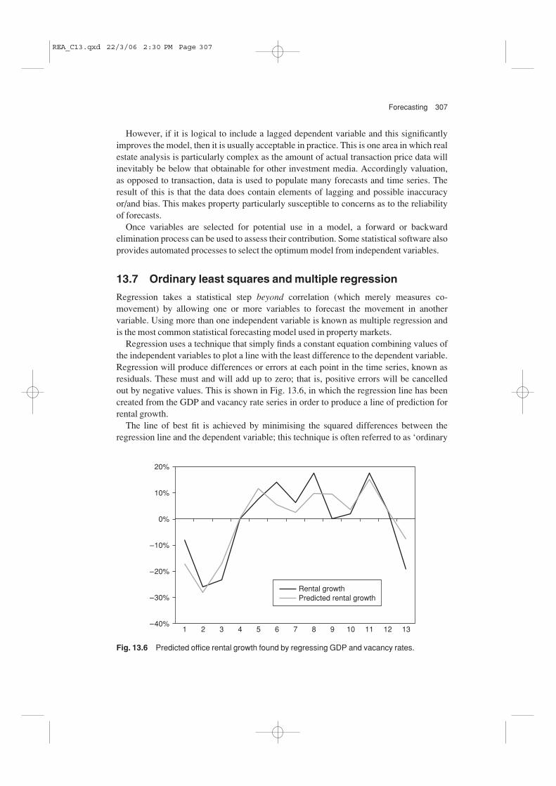
Forecasting 307

However, if it is logical to include a lagged dependent variable and this significantlyimproves the model, then it is usually acceptable in practice. This is one area in which realestate analysis is particularly complex as the amount of actual transaction price data willinevitably be below that obtainable for other investment media. Accordingly valuation, as opposed to transaction, data is used to populate many forecasts and time series. Theresult of this is that the data does contain elements of lagging and possible inaccuracyor/and bias. This makes property particularly susceptible to concerns as to the reliability of forecasts.

Once variables are selected for potential use in a model, a forward or backward elimination process can be used to assess their contribution. Some statistical software alsoprovides automated processes to select the optimum model from independent variables.

13.7 Ordinary least squares and multiple regression

Regression takes a statistical step beyond correlation (which merely measures co-movement) by allowing one or more variables to forecast the movement in another variable. Using more than one independent variable is known as multiple regression and is the most common statistical forecasting model used in property markets.

Regression uses a technique that simply finds a constant equation combining values ofthe independent variables to plot a line with the least difference to the dependent variable.Regression will produce differences or errors at each point in the time series, known asresiduals. These must and will add up to zero; that is, positive errors will be cancelled out by negative values. This is shown in Fig. 13.6, in which the regression line has beencreated from the GDP and vacancy rate series in order to produce a line of prediction forrental growth.

The line of best fit is achieved by minimising the squared differences between theregression line and the dependent variable; this technique is often referred to as ‘ordinary

20%

10%

0%

–10%

–20%

–30%

–40%1 2 3 4 5 6 7 98 10 11 12 13

Rental growthPredicted rental growth

Fig. 13.6 Predicted office rental growth found by regressing GDP and vacancy rates.

REA_C13.qxd 22/3/06 2:30 PM Page 307


least squares’ (OLS). There are other regression methods, such as weighted least squares,that have uses in specific situations where OLS regression is not the most appropriatemethod.

The equation of the regression line comprises a constant (or intercept) and a coefficient(or slope) for each independent variable. As the equation does not fit the dependent variable exactly, there is also an error term. The dependent variable is usually referred to as the y variable and the independent variables as the x variables. The equation takes the form shown below with a further coefficient for each independent variable:

Y = constant + (coefficient × X) + error

13.7.1 Regression statistics

Spreadsheet packages such as Microsoft Excel contain functions to calculate regressionlines that produce results on the accuracy of the model. Table 13.2 shows the output for the regression equation used to produce the predicted rental growth line in Fig. 13.6. Themultiple ‘R’ statistic is simply the correlation coefficient between the dependent variableand the predicted series with values ranging from −1 to +1. The R squared statistic takesthe correlation coefficient one stage further by identifying the proportion of variance in the dependent variable that can be explained by the regression equation. The remainingelement is that which is unexplained between the two variables.

Adding more variables to the regression analysis will never reduce the R squared; it willeither stay the same or increase. The adjusted R squared measure takes account of thenumber of independent variables – in simple terms, more independent variables reduce the

Table 13.2 Output for regression equation.

(a) Summary output

Multiple R 0.8917R squared 0.7952Adjusted R squared 0.7542Standard error 0.0731Observations 13

(b) ANOVA

df SS MS F Significance F

Regression 2 0.2073 0.1036 19.4119 0.0004Residual 10 0.0534 0.0053Total 12 0.2607

Coefficients Standard error t Stat P-value Lower 95% Upper 95%

Intercept 0.0477 0.1152 0.4145 0.6873 −0.2089 0.3044Vacancy rate −1.3279 0.6497 −2.0439 0.0682 −2.7754 0.1197GDP 4.5050 2.1757 2.0706 0.0652 −0.3428 9.3528

REA_C13.qxd 22/3/06 2:30 PM Page 308

Forecasting 309

confidence you can have in the results. The R squared and adjusted R squared will be thesame for models with one independent variable, but for multiple regression equations the adjusted figure is the best measure of overall model accuracy.

The standard error is the standard deviation of the points in the regression line from the dependent variable. Like the standard deviation, it can be used to form confidenceintervals around the forecasts produced by the regression equation.

The significance and reliability of each coefficient, and therefore each independent variable, is determined by the so-called ‘t’ statistic. It is outside the scope of this book togive a detailed analysis of this and other statistics but, as a rule of thumb, a ‘t’ statisticshould be more than +2 or less than −2 to be significant, although the actual figure willdepend on the number of observations in the time series minus the number of parametersestimated. This figure is known as the degrees of freedom. In this case it is 13 minus the two independent variables and constant, summing to 10. The actual figure for the ‘t’ statistic at different levels of confidence can be found in statistical tables. In some packages, an ‘F’ statistic may also be shown; this is the square of the ‘t’ statistic.

Another important measure is the P, or probability value. This measures the probabilitythat the coefficient is actually zero and therefore not significant in the model. A 95%confidence interval would mean that the P value needs to be less than 0.05. Whilst a greateror lesser level of probability may be acceptable, depending on the circumstances, 95% iscommonly adopted as the acceptable level of probability.

The confidence intervals show the range within which you would be 95% confident that the coefficients fell. A smaller confidence interval is better. MS Excel allows you tospecify different levels of confidence for this measure.

13.7.2 Interpretation of regression results

The first point to draw out from examination of the example is that the overall model accuracy is good, with 75% of the variance in rental growth explained by the model.However, there are some problems with the ‘t’ statistics and P values.

It is often the case that the ‘t’ statistic on the intercept/constant is not significant. How-ever, unless there is a structural or theoretical reason to remove it the constant is left in, although MS Excel does give you the option to have the constant at zero. Removing theconstant can lead to violating the assumption that error terms sum to zero by biasing the intercept. In a perfect world the intercept would be zero as all relevant independentvariables would be included, alleviating any bias in the regression line.

Using statistical tables both ‘t’ statistics are significant at 90% confidence level with 10 degrees of freedom (1.81), but not significant at 95% (2.23). This may be due to multi-collinearity between the variables as a result of their high correlation. In practice, youwould try other variables that might work better in combination with the GDP and vacancyrate data and therefore produce significant ‘t’ statistics at 95% confidence.

The equation for the regression line at each point in the time series will be:

Predicted rental growth = 0.0477 + (Vacancy rate × −1.3279) + (GDP × 4.5050)

Forecasts of the rental growth time series can then be projected by substituting future estimates of vacancy rate and GDP into the above equation.

REA_C13.qxd 22/3/06 2:30 PM Page 309


It should be noted that the error term is calculated as the difference between the predicted rental growth and actual rental growth so that:

Rental growth = Predicted rental growth + Error

13.8 Diagnostic tests

To check whether the model estimated conforms to the five assumptions outlined earlier inthe chapter, diagnostic tests should be run to identify problems such as:

• Heteroskedasticity: the error terms’ variance is not constant through time, indicatingthat the model’s accuracy is varying through time.

• Autocorrelation: the error terms have a trend indicating that the model is more accurateat some points in time than at others.

• Outliers: reduce the goodness of fit of the regression line.

• Multicollinearity: two or more independent variables are highly correlated.

While these tests can be carried out in MS Excel, the use of specialised econometrics packages such as E-Views, which have many tests as built in functions, will be preferred if this level of sophistication is required on a regular basis.

13.9 The use of forecasts

The forecasting techniques examined in this chapter are only valuable tools if they areused to provide insight and help forecasters to make more informed judgements. While the techniques are sophisticated, they are susceptible to the GIGO (garbage in, garbageout) syndrome. Forecasting is therefore part science, part art.

The first thing that anyone using forecasts based on statistical techniques should consider is that they are not point estimates: they are probability distributions. The figurecalculated from regression analysis is in the centre of the probability distribution. Unlessyou know the confidence and potential for error in forecasts, you cannot make informeddecisions from them. Furthermore, if forecasts of independent variables are used to forecast the dependent variable, as will often be the case, it is inevitable that the potentialfor error in the forecast is increased.

13.10 Forecast equations and their calibration

A variety of quantitative forecasting models are used in the commercial property market.These range from simple to complex techniques and include:

• Single equation models, which include variables such as GDP, employment levels andfinancial variables in order to forecast rental growth, returns or yields.

• ‘Inter-active’ simultaneous equation models, which can be described as behavioural orstructural models.

The aim of the forecasting model builder is to identify those models that produce usefuland superior results. This task needs experience and expertise. The modeller should be

REA_C13.qxd 22/3/06 2:30 PM Page 310

Forecasting 311

aware of the characteristics and quality of the data used. A feature of many property models is that they incorporate data and information relating to the general economy andbusiness conditions. These tend to be openly available, but at a cost, and can provide use-ful early signals: for example, consumer spending, output, employment (Matysiak, 1997).

Many forecasters seek to identify key variables that pick up changes in rental values. In practice, it has been found that the set of explanatory variables varies by sector. In the office sector, for example, it has been found that the gross domestic product, output and employment in financial and business services, unemployment, interest rates andoperating expenses produce the highest statistical relationships. Consequently, it is thesevariables that are built into the models.

The vacancy rate is thought by many to play an important role. The logic is that if thevariables that affect vacancy rate can be identified, then as the vacancy rate affects rentalgrowth, a model can be constructed. In particular, it is the gap between actual vacancy rate and structural vacancy rate that matters (Hendershott et al., 1999).

In the retail sector expenditure, lagged retail profits and the GDP seem to be the mostsuccessful demand side indicators. In the industrial market, the GDP and manufacturingoutput seem to be the most significant variables in the UK literature (RICS, 1994;Thompson and Tsolacos, 1999, 2001). Attempts to incorporate supply side variables in themodels have generally not worked, and this quest has been hindered by the discontinuationof the official HMSO (now TSO) floor space data.

Regression analysis (as described earlier in the chapter) is one approach that can be use-ful in helping to identify the relationships in the underlying data. The aim with regressionequations is to find the regression figures that produce the highest coefficient of determina-tion, R2, for an appropriate lead-lag period. In regression models, the set of variables maybe split into soft/financial and hard indicators. For each of these categories, individualseries are ranked according to their explanatory power as measured by the R2 statistic froma bivariate regression between the variable of interest yt, such as rental growth or take-up,and the individual indicator (denoted xi,t) in which the retained lag of the indicator isselected automatically according to statistical criteria. This is summarised as:

∆ ln(y)t = β(L)ixi,t + εi,t

In this equation, we seek to explain and/or anticipate changes in variables, such as rentalgrowth or take-up, by using variables that lead rental growth or take-up.

Based on work undertaken by Matysiak, examples of some economic/financial vari-ables that have been found to be useful in forecasting various property variables such asrental growth or investment yields at the sector level are shown in Table 13.3 (Matysiakand Tsolacos, 2003). In forecasting models, these variables are often useful at highlyaggregated levels: for example, at the retail, office or industrial sector level. However, inorder to forecast local market movements for rental growth, yield changes or take-up, localdata is required.

13.11 Property market barometers and lead indicators

Property forecasters tend to use sophisticated modelling techniques; however, propertymarket barometers are relatively straightforward in their construction. Barometers provide

REA_C13.qxd 22/3/06 2:30 PM Page 311


real estate decision-makers with an indicator of market trends and sentiment, and can helpforecasters to identify turning points in the market. Barometers gather the current views of key players as to say yield or rental value movements. They give a market view as at apoint in time.

In contrast, lead indicators seek to identify data series that are statistically linked to theway in which the market will move. The benefit of identifying lead indicators has beenreiterated by Matysiak and Tsolacos (2003). Lead indicators are viewed as being particularly useful to analysts involved in DCF appraisals in helping to clarify their cashflow projections. Examples of lead indicators are changes in:

• lease length;

• roll-over percentages (percentage of tenants that renew their leases);

• break options;

• time vacant space is on the market;

• volume of investment transactions.

Individual lead indicators may be combined in order to produce a composite measure thatis likely to provide a more reliable indicator of future market conditions.

When regression-based forecast models are used, their accuracy may be enhanced by the inclusion of a composite lead indicator. This composite indicator would con-sist of timely local property data, appropriately weighted (Matysiak and Tsolacos, 2003).

13.12 The role of forecasts in financial and property lending markets – value at risk

In this section consideration is given to two areas where forecasting expertise and riskanalysis skills are becoming increasingly important. These are ‘value at risk’ and stresstesting. Both are tools to assist in the risk management of assets.

Every investor would like to reduce or eliminate risk; however, to do so is not possiblenor would it be consistent with the need to achieve a satisfactory level of return. If this isaccepted then it is risk measurement and risk management that become the key concerns,within which forecasting has a distinct role. Additionally, the development of risk man-agement techniques that rely on estimates of the future may be expected to have a growing

Table 13.3 Economic financial variables.

Gilts yields Car registrations Net lending to consumersExport orders Volume of expected output Financial surplus/deficitConsumer confidence Stock of finished goods Real money supply M4Changes in inventories Consumer credit Personal disposable incomeIndustrial production Unit labour costs Gross trading profitsHouse building starts Yield curve Manufacturing investmentReal money supply M0 Press recruitment ads Private to total creditNew orders in manufacturing FT All Share Price Index Manufacturing outputManufacturing employment Retail sales Gross domestic product

REA_C13.qxd 22/3/06 2:30 PM Page 312

Forecasting 313

impact on both the scope and depth of the skills base required in the property market. In particular, it is likely that the skills offered by accomplished forecasters, who tend to be few and far between, will became increasingly sought after.

A role of forecasts is to identify future performance patterns for properties and portfolios. Where the property assets are highly geared, the equity investor can be exposedto downturns in the markets. The worry for equity investors and the banks financing themwill be their exposure to downside risk or losses.

Value at risk is a measure developed by J.P. Morgan with a view to establishing a market standard. They released their value at risk model under the badging ‘RiskMetrics’as long ago as 1994. The RiskMetrics software program contains simplified risk assess-ment calculations and provided an important impetus to the growth in the use of value atrisk amongst smaller financial institutions, non-financial corporations and institutionalinvestors. In particular, its appeal was amongst the major derivatives dealers for measur-ing and managing market risk.

Value at risk is a single, summary, statistical measure of possible portfolio losses. It is a measure of losses that might be expected as a result of ‘normal’ market movements. The model identifies the size of the (normally) small probability where losses greater than the value at risk might be suffered. The underlying concept of value at risk can be summarised as a way to describe the magnitude of the likely losses to the portfolio.

Value at risk is not a cure-all. It is a single, summary, statistical measure of normal market risk to which the company is exposed. The value at risk numbers will frequently be supplemented by the results of other risk measures: for example, scenario analyses andstress testing.

Stress testing is also important in forecasting risk. It often begins with a set of hypothet-ical extreme market scenarios. These scenarios might be created from predeterminedextreme scenarios (such as the market moving by five or ten standard deviations from its central tendency) for each of the sectors in which the business operates. The linkage(correlation) between potential losses is considered and an overall picture is gained of howthe investment or banking activities might fare under extreme conditions. The propertymarket has endured a number of cycles, the two worst of which in recent times wereobserved to bottom in 1973 and 1990. If property losses are correlated to other financiallosses at such points in time, the bank may find its capital adequacy ratios under pressure.Value at risk seeks to identify these cross-relationships and the point at which marketmovements could place a financial institution in jeopardy.

There are alternatives to value at risk, as value at risk may not be appropriate for all entities. The two alternative methodologies are sensitivity analysis and cash flow at risk.Sensitivity analysis (discussed in Chapter 8) is less sophisticated than value at risk. In contrast, cash flow at risk can be considered more sophisticated than value at risk. Cash flow at risk focuses on the robustness of cash flows rather than changes in market-to-market values. Cash flow at risk measures are typically estimated using simulation techniques and focus on a longer time horizon than value at risk measures.

Such techniques are currently rarely seen in the real estate market. However, they areestablished within the financial and business communities, and professionals operating inthe real estate investment market should be aware of how competing markets deal withestimating the exposure to market risks in a future context.

REA_C13.qxd 22/3/06 2:30 PM Page 313


Additionally, for those involved in property lending, the Basle Capital Accord is bring-ing risk measurement and forecasting techniques onto the ‘radar screen’. The implicationsof this are now explained.

13.13 Basle Capital Accord

Under the Basle Capital Accord agreement and related banking supervisory regulations,banks are required to have minimum capital adequacy ratios. These ratios measure therelationship between the bank’s equity base (regulatory capital) and the size of its loanbook. Principle I of the Accord requires banks to have a capital requirement of 8% forcredits (loans) granted. Thus equity of 8 is required to support loans granted of 100. Thefigure for pure real estate loans is reduced to 50%, giving a capital requirement of 4% of the amount loaned. Where a bank fails to meet the necessary capital adequacy ratio it isnot normally able to operate in the inter-bank money markets, and this seriously impedes it ability to undertake business.

In due course, a further tightening of capital adequacy regulations is envisaged with a second accord, known as Basle II. The objective is to get banks to undertake several different approaches for calculating how sensitive their regulatory capital base is to the degree of risk in individual financing transactions. The Basle Committee on Banking Supervision, a division of the Bank for International Settlements (BIS), is currently working on a completely new capital accord for credit institutions. After an initial consultation phase, there are plans to bring into force the new Basle II Capital Accord with effect worldwide from a likely date in 2008/9 for all internationalbanks.

Basle II will place a greater onus on banks to calculate and manage their risk positions,in the context of the size of their capital base. The risk rating would serve as the basis forcalculating the bank’s capital requirements, along with the associated probability ofdefault. As a result, the risk structures of individual financing transactions will have amuch stronger influence on margin amounts in the future.

In summary, Basle II proposals comprise three regulatory areas, to which banks will berequired to adhere if they wish to operate freely in the inter-bank money markets. First,there is the prospect of the introduction of differentiated credit risk assessment, requiringthat operational and other banking risks must be re-analysed, measured, and backed with regulatory capital; second, banks would be required to comply with supervisoryrequirements relating to their reporting requirements; and third, to adhere to stringent legal disclosure obligations.

The fundamental view put across by the Committee on Banking Supervision is thatworldwide minimum capital requirements should remain unchanged, at an average of 8%for all banks. The extent to which Basle II will call for this average to be raised or loweredin the context of a bank’s specific loan portfolio and other derivative or investment exposures is likely to be based on:

• the loan portfolio structure of each individual institution;

• the structure and risk degree of the individual financings; and

• how the individual bank overcomes operational and other risks.

REA_C13.qxd 22/3/06 2:30 PM Page 314

Forecasting 315

In calculating capital requirements, Basle II thus calls for the consideration of bank-specific factors, in addition to those of the individual transactions. Basle II pro-vides for the use of external credit ratings for banks and, as many banks are unrated, it also provides for the use of internal ratings determined by the bank itself. The internal ratings will determine default probabilities and use them as the basis for the rating grades.

13.13.1 Real estate implications flowing from Basle II

The advent of Basle II will place additional requirements on banks when undertaking lending. That much is certain. Real estate underpins a significant proportion of bank loantransactions. The prospective thrust for real estate will be the requirement for more thanjust valuations for loan purposes. A requirement for prospective cash flow ratios – for example, long-term debt service cover ratios – will require forecasting expertise in a property-specific context. Also, property and property debt will need to be placed into a portfolio context.

The risk assessment techniques that are proposed under Basle II, and the requirement toprovide cash flow forecasts in the context of prospective debt service cover ratios, willbring the risk and cash flow forecasting methodologies of the financial markets into thewings of the property marketplace. This in turn will require an increase in appropriateskills amongst the property adviser community.

13.14 Summary and conclusions

In this chapter the forecasting methods used within the property market have beenexplored and placed into the context of the wider capital markets.

Forecasting methodologies employed in the financial markets by econometricians tendto be complex in nature and beyond the knowledge and skills base of many in the realestate marketplace. In the past there was a good reason for this. Those who operate withinthe financial markets have long had access to substantial data series (daily, weekly ormonthly). In stark contrast, forecasters operating in the real estate markets have two issuesthat make accurate or meaningful forecasting significantly more difficult. Primarily, these relate to the paucity of data that exists. Data series within the direct property markettend to be at best monthly, and frequently quarterly or even annually. Matters are further complicated in that whilst in the equities market the main indices are transaction based, in the property market the indices are appraisal- (or valuations-) based (Matysiak and Wang, 1995). Furthermore, the fact that a number of the commonly used data seriesexhibit non-stationarity provides another complication.

When considering property forecasts, care should be taken to understand the drivers ofthe model employed and the sensitivities of the outputs of the model to the input variables.In practice, forecasting models require calibration and need to be set against that whichagents are seeing happen or are expecting to see happen in the short term.

In conclusion, property forecasting currently suffers from an inadequacy of both appropriate skills and data. Great strides have been made in terms of the latter in recentyears; it is incumbent on practitioners and analysts to address the former.

REA_C13.qxd 22/3/06 2:30 PM Page 315


ReferencesAdams, A., Booth, P., Bowie, D. and Freeth, D. (2003) Investment Mathematics. London: Wiley

Finance/John Wiley & Sons Ltd.Darnell, A.C. (1994) A Dictionary of Economics. Aldershot: Edward Elgar.Hendershott, P., Lizieri, C. and Matysiak, G. (1999) Workings of the London office market. Real

Estate Economics, 27 (2): 365–87.Matysiak, G. (1997) Modelling and forecasting in commercial property. Editorial. Journal of

Property Finance, 8 (4).Matysiak, G. and Tsolacos, S. (2003) Identifying short-term leading indicators for real estate rental

performance. Journal of Property Investment & Finance, 21 (3): 212–32.Matysiak, G. and Wang, P. (1995) Commercial property market prices and valuations: analysing the

correspondence. Journal of Property Research, 12 (3): 181–202.Myer, N. and Webb, J. (1993) Return properties of equity REITs, common stocks and commercial

real estate: a comparison. Journal of Real Estate Research, 8 (1): 87–106.Newell, G., Matysiak, G. and Venmore-Rowland, P. (1997) Do property company shares perform in

the same way as the property market? London: RICS Foundation Publication.Royal Institution of Chartered Surveyors (1994) Understanding the Property Cycle: Economic

Cycles and Property Cycles. London: RICS.Royal Institution of Chartered Surveyors (2003) Appraisal and Valuation Standards. London:

RICS.Sims, C. (1972) Money, income and causality. American Economic Review, 62 (4): 540–52.Sims, C. (1980) Macroeconomics and reality. Econometrica, 48 (1).Thompson, R. and Tsolacos, S. (1999) Rent adjustments and forecasts in the industrial markets.

Journal of Real Estate Research, 17 (1/2): 151–67.Thompson, R. and Tsolacos, S. (2001) Industrial land values – a guide to future markets? Journal of

Real Estate Research, 21 (1/2): 55–67.

REA_C13.qxd 22/3/06 2:30 PM Page 316

1 value and worth Introducing concepts of - Wiley-Blackwell · Introducing concepts of 1 value and...

Documents

Transcript of 1 value and worth Introducing concepts of - Wiley-Blackwell · Introducing concepts of 1 value and...