1 of 39 The EPA 7-Step DQO Process Step 7 - Optimize Sample Design DQO Case Study 45 minutes...
39
1 of 39 The EPA 7-Step DQO Process Step 7 - Optimize Sample Design DQO Case Study 45 minutes Presenter: Sebastian Tindall DQO Training Course Day 3 Module 20
-
Upload
rosalind-richardson -
Category
Documents
-
view
263 -
download
7
Transcript of 1 of 39 The EPA 7-Step DQO Process Step 7 - Optimize Sample Design DQO Case Study 45 minutes...

1 of 39
The EPA 7-Step DQO Process
Step 7 - Optimize Sample DesignDQO Case Study
45 minutes
Presenter: Sebastian Tindall
DQO Training CourseDay 3
Module 20

2 of 39
Information IN Actions Information OUT
From Previous Step To Next Step
Select the optimal sample size that satisfies the DQOs for each data collection design option
For each design option, select needed mathematical expressions
Check if number of samples exceeds project resource constraints
Decision Error Tolerances
Gray Region
Optimal Sample Design
Go back to Steps 1- 6 and revisit decisions. Yes
No
Review DQO outputs from Steps 1-6 to be sure they are internally consistent
Step 7- Optimize Sample Design
Develop alternative sample designs

3 of 39
Terminal Objective
To be able to use the output from the previous DQO Process steps to select sampling and analysis designs and understand design alternatives presented to you for a specific project

4 of 39
Sampling Approaches
Sampling Approach 1– Simple Random
– Traditional fixed laboratory analyses
Sampling Approach 2– Systematic Grid
– Field analytical measurements
– Computer simulations
– Dynamic work plan
5 of 39
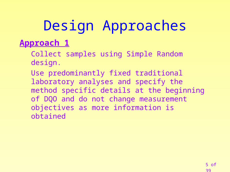
Design ApproachesApproach 1
Collect samples using Simple Random design.
Use predominantly fixed traditional laboratory analyses and specify the method specific details at the beginning of DQO and do not change measurement objectives as more information is obtained

6 of 39
Approach 1 Sample Design
Plan View
Former PadLocation
RunoffZone
0 50 100 150 ft0 15 30 46 m
BufferZone

7 of 39
Histogram
0
1
2
3
0 7 14 21 28 35
Pb Concentration (mg/kg)
Fre
qu
en
cy
0
1
2
3
4
0 85 95 105 115
U Concentration
Fre
qu
en
cy0
1
2
3
4
0 1.7 3.4 5.1 6.8
TPH Concentration
Fre
qu
en
cy
0
1
2
3
0 0.8 1.6 2.4 3.2
Arochlor 1260
Fre
qu
en
cy

8 of 39
“Normal” Approach
Due to using only five samples for initial distribution assessment, one cannot infer a ‘normal’ frequency distribution
Reject the ‘Normal’ Approach and Examine ‘Non-Normal’or ‘Skewed’ Approach

9 of 39
Pb, U, TPH (DRO/GRO) Because there were multiple COPCs with
varied standard deviations, action limits and LBGRs, separate tables for varying alpha, beta, and (LBGR) delta were calculated
For the U, Pb, and TPH, the largest number of samples for a given alpha, beta and delta are presented in the following table

10 of 39
Pb, U, TPH Based on Non-Parametric TestSample Sizes Based on Varying Error Tolerances and LBGR
Lead, Uranium, and TPH
Mistakenly Concluding < Action Level
s = 10.5 (U) = 0.01 = 0.05 = 0.10
Sample size formula: 2)(
)(16.1
12
2
2211
n
Width of the Gray Region, () = 240 – 229.5 = 10.5 (total error estimate)
= 0.10 19 12 9
= 0.20 15 9 7
Mis
tak
enly
C
oncl
ud
ing
> A
ctio
n
Lev
el
= 0.30 13 8 5
Width of the Gray Region, () = 240 – 192 = 48 (20% of action level)
= 0.10 4 3 2
= 0.20 4 2 2
Mis
tak
enly
C
oncl
ud
ing
> A
ctio
n
Lev
el
= 0.30 4 2 2
Width of the Gray Region, () = 240 – 120 = 120 (50% of action level)
= 0.10 4 2 2
= 0.20 4 2 1
Mis
tak
enly
C
oncl
ud
ing
> A
ctio
n
Lev
el
= 0.30 4 2 1
11 of 39
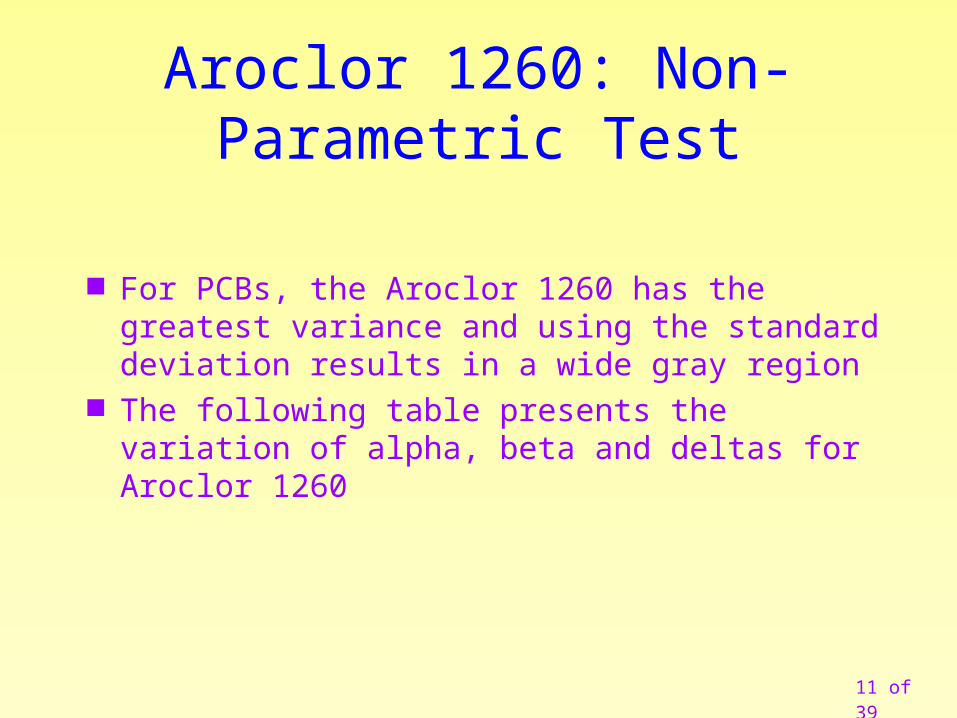
Aroclor 1260: Non-Parametric Test
For PCBs, the Aroclor 1260 has the greatest variance and using the standard deviation results in a wide gray region
The following table presents the variation of alpha, beta and deltas for Aroclor 1260

12 of 39
Aroclor 1260: Non-Parametric TestSample Sizes Based on Varying Error Tolerances and LBGR
PCBs (based on Aroclor 1260)
Mistakenly Concluding < Action Level
s = 0.88 (A-1260) = 0.01 = 0.05 = 0.10
Sample size formula: 2)(
)(16.1
12
2
2211
n
Width of the Gray Region, () = 1 – 0.12 = 0.88 (total error estimate)a
= 0.10 19 12 9
= 0.20 15 9 7
Mis
tak
enly
C
oncl
ud
ing
> A
ctio
n
Lev
el
= 0.30 13 8 5
Width of the Gray Region, () = 1 – 0.80 = 0.20 (20% of action limit)
= 0.10 296 194 149
= 0.20 229 141 103
Mis
tak
enly
C
oncl
ud
ing
> A
ctio
n
Lev
el
= 0.30 186 108 75
Width of the Gray Region, () = 1 - 0.50 = 0.50 (50% of action limit)
= 0.10 50 33 25
= 0.20 40 24 18
Mis
tak
enly
C
oncl
ud
ing
> A
ctio
n
Lev
el
= 0.30 33 19 13
a The total error estimate for subsurface concentrations exceeds the action limit, thus inappropriately moving the LBGR below zero. Only the surface concentration error estimate is considered here for that reason.

13 of 39
Approach 1 Sampling Design (cont.) Surface Soils S&A Costs
Lab Analytical Cost Without PCBs
Unit Sample Analysis Cost
Pb by ICP/AES $35U by ICP/AES $65TPH (GRO) by GC $65TPH (DRO) by GC $85
Total USA$ $250
Unit Sample Collection Cost $50AUSCA$ = USC$ + total USA$ $300

14 of 39
Approach 1 Sampling Design (cont) Sub-surface Soils S&A Costs

15 of 39
Approach 1 Sampling Design (cont.)
Surface Soils
Lab Analytical Costs for PCBs by GCPolychlorinated biphenyls 150.00$
Total USA$ 150.00$ Unit Sample Collection Cost 50.00$ AUSCA$ = USC$ + total USA$ 200.00$
16 of 39
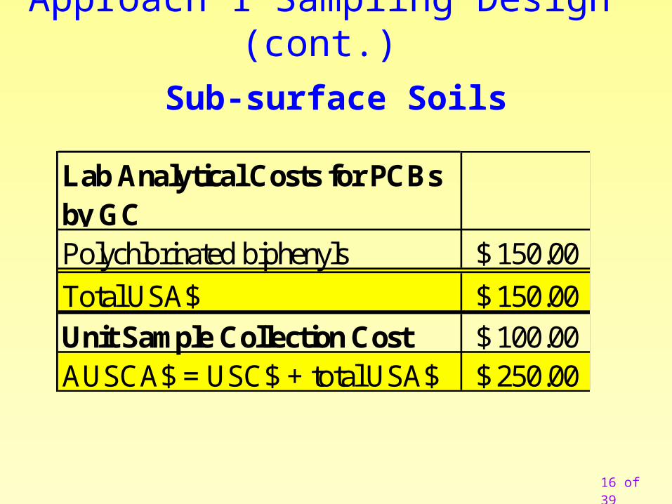
Approach 1 Sampling Design (cont.)
Sub-surface Soils
Lab Analytical Costs for PCBs by GCPolychlorinated biphenyls 150.00$
Total USA$ 150.00$ Unit Sample Collection Cost 100.00$ AUSCA$ = USC$ + total USA$ 250.00$

17 of 39
Approach 1 Based Sampling Design Design for Pb, U, TPH
– Alpha = 0.05; Beta = 0.2; Delta = total error
– The decision makers agreed on collection of 9 surface samples for Pb, U and TPH (GRO & DRO) from each of the two surface strata, for a total of 18 samples using a stratified random design
– For the sub-surface, nine borings/probes will be collected from each of the two subsurface stratum at random locations, collected at a random depth down to 10 feet, to assess migration through the vadose zone, for a total of 18 samples
Design for PCBs– Alpha = 0.05; Beta = 0.20; Delta = 0.50 (50% of the AL)
– The decision makers agreed on collection of 24 surface samples from each of the two surface strata; total of 48 samples using a stratified random design
– For the sub-surface, 24 borings/probes will be collected from each of the two subsurface stratum at random locations, collected at a random depth down to 10 feet for a total of 48 samples (2 X 24)

18 of 39
Approach 1 Sample Locations(Surface Strata)
Plan View
Former PadLocation
RunoffZone
0 50 100 150 ft0 15 30 46 m
BufferZone

19 of 39
Approach 1 Sampling Design (cont.)

20 of 39
Remediation Costs*
*Does not include layback area
DR#
Description/Depth Area(ft2)
Volume(yd3)
Cost*
1a Pad & Run-off Zone, 0-6” 12,272 227 $45,4001b Buffer Zone (excluding
Pad and Run-off area), 0-6”42,884 794 $158,800
2a Pad & Run-off Zone,6”-10”
12,272 4,318 $863,600
2b Buffer Zone (excludingPad and Run-off area),6”-10”
42,884 15,089 $3,017,800
* Assume $200 per yd3 for all COPCs

21 of 39
Approach 1 Based Sampling Design Compare Approach 1 costs versus remediation
costs – Approach 1 S&A costs
• $11,700 (Pb, U, TPH) + $21,600 (PCBs) = $33,300
– Remediation costs• Cost to remediate surface soil under footprint of pad and
buffer area: $204,200• Cost to remediate subsurface soil under footprint of pad and
buffer area: $3,881,400

22 of 39
Design ApproachesApproach 2: Dynamic Work Plan (DWP) & Field Analytical Methods (FAMs)
Manage uncertainty by increasing sample density by using field analytical measurementsManage uncertainty by including RCRA metals as COPCs Use DWP to allow more field decisions to meet the measurement objectives and allow the objectives to be refined in the field using DWP

23 of 39
Approach 2 Sampling Design
Phase 1: Pb, U, TPH, PCBs– Perform field analysis of the four strata on-site using XRF
(RCRA metals & U), on-site GC (TPH), and Immunoassay (PCBs) methods. Take into account the chance of false positives at the low detection levels
– This will produce a worse-case frequency distributions and variance for each COPC that will be used to select the proper statistical method and then calculate the number of confirmatory samples for laboratory analysis for the surface and below grade strata

24 of 39
Phase 1: Metals, TPH, PCBs– Provide detailed SOPs for performance of FAMs: XRF,
GC, & Immunoassay analysis– Divide both surface strata into triangular grids– Use systematic sampling, w/random start (RS), to locate
sample points; sample in center of each grid Pad & Run-off zone
– CSM expects contamination more likely here– 10 ft equilateral triangle: 43.35 ft2
– Pad + Run-off zone = 12,272 ft2
– 283 sample points
Buffer area: – Also 283 sample points – CSM expects contamination less likely here– Thus, grid triangle has larger area
Approach 2 Sampling Design (cont.)

25 of 39
Phase 1: Pb, U, TPH, PCBs– Sub-surface strata: Pad & Run-off zone
Use Direct Push Technology (DPT) to collect Push at all surface sample points > ALs Minimum sample locations: 40 (+ 10 >ALs) = ~50 Collect sub-surface samples at 3-7-10 feet 50 X 3 = 150 sub-surface samples in this strata Use systematic sampling, w/random start (RS), to locate sample
points
– Buffer area CSM expects contamination less likely here Thus, fewer sample points Same >ALs rationale as above 50 X 3 = 150 sub-surface samples in Buffer area Use systematic sampling, w/RS, to locate sample points
Approach 2 Sampling Design (cont.)
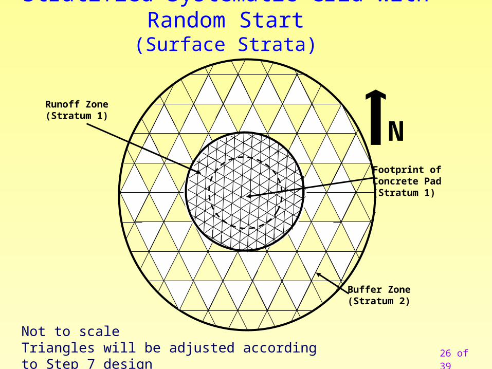
26 of 39
Stratified Systematic Grid with Random Start(Surface Strata)
Not to scaleTriangles will be adjusted according to Step 7 design
NFootprint ofConcrete Pad(Stratum 1)
Runoff Zone(Stratum 1)
Buffer Zone(Stratum 2)
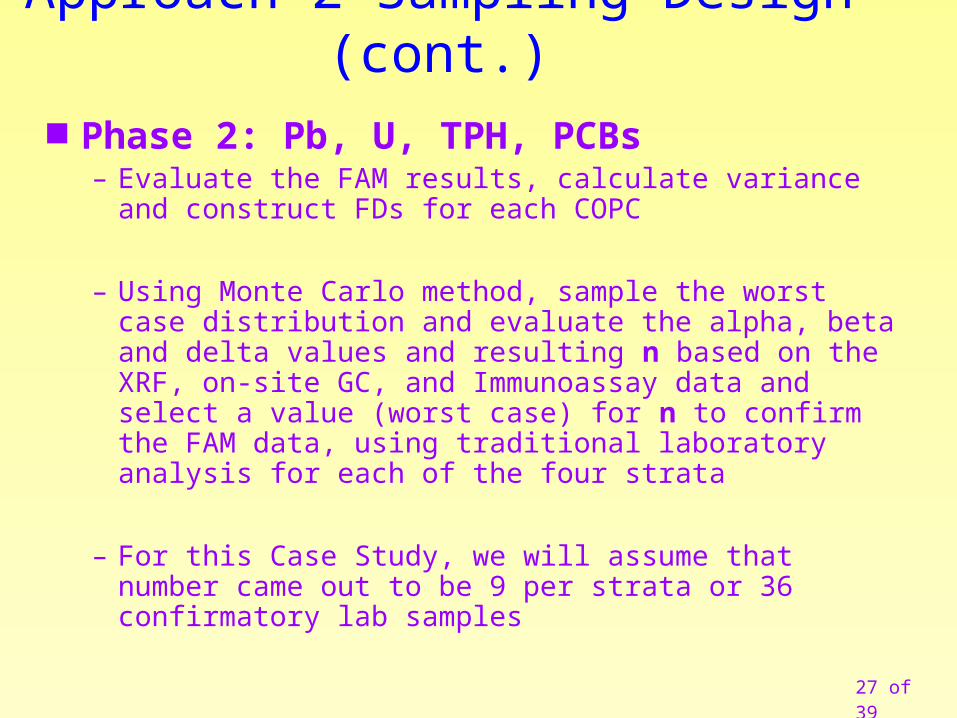
27 of 39
Phase 2: Pb, U, TPH, PCBs– Evaluate the FAM results, calculate variance and construct
FDs for each COPC
– Using Monte Carlo method, sample the worst case distribution and evaluate the alpha, beta and delta values and resulting n based on the XRF, on-site GC, and Immunoassay data and select a value (worst case) for n to confirm the FAM data, using traditional laboratory analysis for each of the four strata
– For this Case Study, we will assume that number came out to be 9 per strata or 36 confirmatory lab samples
Approach 2 Sampling Design (cont.)

28 of 39
FAM ProcedureSW-846, Draft Update IVA
Method 6200
Field portable x-ray fluorescence spectrometry for the determination of elemental concentrations in soil and
sediment

29 of 39
FAM ProcedureSW-846, Draft Update III
Method 4020
Screening for polychlorinated biphenyls by immunoassay

30 of 39
FAM Procedure for GROSW-846, Draft Update III
Preparation Method 5030 or 5035(purge and trap methods)
Followed by Analysis Method 8015 B
Non-halogenated organics using GC/FID

31 of 39
FAM Procedure for DROSW-846, Draft Update III
One of Following Extraction Methods:
• 3540 (soxhlet), • 3541(auto-soxhlet),• 3550 (ultrasonic), or• 3560 (super critical fluid)
Followed by Analysis Method 8015 B:• Non-halogenated organics using GC/FID

32 of 39
Approach 2 Sampling Design (cont.)Surface Soils SC&SA Costs
U by Field XRF $2RCRA Metals by Field XRF $12TPH (GRO) on-site GC $25TPH (DRO) on-site GC $25
PCBs by IMA kits $50
Total USA$ $114
Unit Sample Collection Cost $25AUSCA$ = USC$ + total USA$ $139
33 of 39
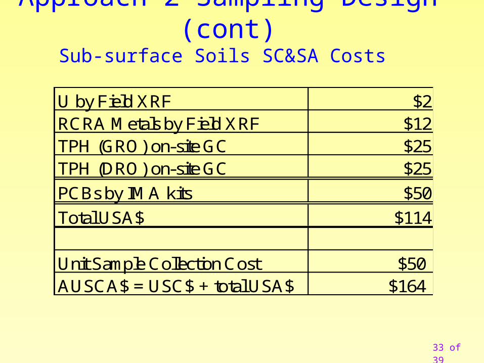
Approach 2 Sampling Design (cont)Sub-surface Soils SC&SA Costs
U by Field XRF $2RCRA Metals by Field XRF $12TPH (GRO) on-site GC $25TPH (DRO) on-site GC $25
PCBs by IMA kits $50
Total USA$ $114
Unit Sample Collection Cost $50AUSCA$ = USC$ + total USA$ $164
34 of 39
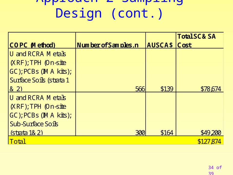
Approach 2 Sampling Design (cont.)
COPC (Method) Number of Samples, n AUSCA$Total SC&SA Cost
U and RCRA Metals (XRF); TPH (On-site GC); PCBs (IMA kits); Surface Soils (strata 1 & 2) 566 $139 $78,674U and RCRA Metals (XRF); TPH (On-site GC); PCBs (IMA kits); Sub-Surface Soils (strata 1&2) 300 $164 $49,200Total $127,874
35 of 39
Number of Samples, n AUSCA$
Total Sampling and Analytical Cost
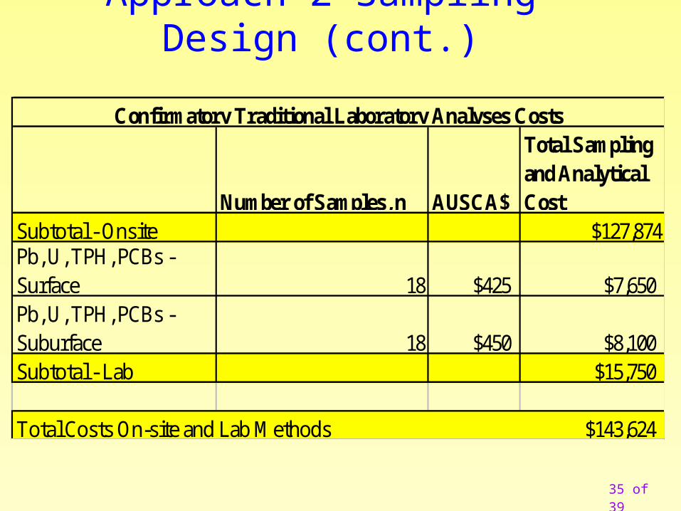
Subtotal - Onsite $127,874Pb, U, TPH, PCBs -Surface 18 $425 $7,650Pb, U, TPH, PCBs - Suburface 18 $450 $8,100Subtotal - Lab $15,750
Total Costs On-site and Lab Methods $143,624
Confirmatory Traditional Laboratory Analyses Costs
Approach 2 Sampling Design (cont.)
36 of 39
Evaluate costs of Approach 2 vs. remediation costs– Sampling and analysis (S&A) costs $143,624– Original budget for S&A $45,000
– Remediation cost Cost to remediate surface soil under footprint of pad and
buffer area: $204,200 Cost to remediate subsurface soil under footprint of pad
and buffer area: $3,881,400
Approach 2 Sampling Design (cont.)
37 of 39
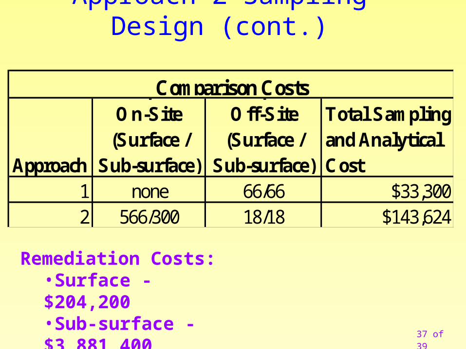
Approach
# Samples, n On-Site
(Surface / Sub-surface)
# Samples, n Off-Site
(Surface / Sub-surface)
Total Sampling and Analytical Cost
1 none 66/66 $33,3002 566/300 18/18 $143,624
Comparison Costs
Remediation Costs:•Surface - $204,200•Sub-surface - $3,881,400
Approach 2 Sampling Design (cont.)

38 of 39
Measure gasoline & diesel range organics (GRO/DRO)
Ship & process all samples in one batch to decrease cost.
QC defined per SW 846 [1 MS/MSD, 1 method blank, 1 equipment blank (if equipment is reused), 1 trip blank for GRO only].
Cool GRO/DRO to 4°C, 2°C. QAP written and approved before implementation.
QC and Analysis DetailsUsed in All Approaches

39 of 39
End of Module 20
Thank you
Questions?