1 Introduction in LabVIEW

8/12/2019 1 Introduction in LabVIEW

http://slidepdf.com/reader/full/1-introduction-in-labview 1/21

Prof.Dr. Doru URSUTIUCVTC – University “TRANSILVANIA” of Brasov

Department of Physics

Graphical Programming

LabVI W

2007

1



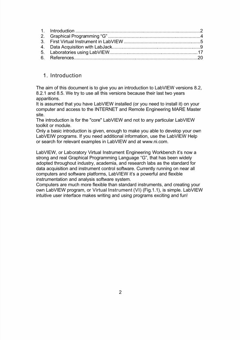
1. Introduction ................................................................................................2 2. Graphical Programming “G” .......................................................................4 3. First Virtual Instrument in LabVIEW ...........................................................5 4. Data Acquisition with LabJack....................................................................9 5. Laboratories using LabVIEW....................................................................17

6. References...............................................................................................20

1. Introduction

The aim of this document is to give you an introduction to LabVIEW versions 8.2,8.2.1 and 8.5. We try to use all this versions because their last two yearsapparitions.It is assumed that you have LabVIEW installed (or you need to install it) on yourcomputer and access to the INTERNET and Remote Engineering MARE Mastersite.The introduction is for the "core" LabVIEW and not to any particular LabVIEWtoolkit or module.Only a basic introduction is given, enough to make you able to develop your ownLabVEIW programs. If you need additional information, use the LabVIEW Helpor search for relevant examples in LabVIEW and at www.ni.com.

LabVIEW, or Lab oratory Virtual Instrument Engineering Workbench it’s now astrong and real Graphical Programming Language “G”, that has been widelyadopted throughout industry, academia, and research labs as the standard fordata acquisition and instrument control software. Currently running on near allcomputers and software platforms, LabVIEW it’s a powerful and flexibleinstrumentation and analysis software system.Computers are much more flexible than standard instruments, and creating yourown LabVIEW program, or Virtual Instrument (VI) (Fig.1.1), is simple. LabVIEWintuitive user interface makes writing and using programs exciting and fun!

2



Fig. 1-1 A simple Virtual Instrument VI (Advanced Harmonic Analyzer)

The terms Virtual Instrument and Virtual Lab supposes both creating someapplications which can simulate certain phenomena or processes (physical,chemical, biological, technological, mathematical…) and introducing the conceptsof “virtual instrumentation” and “computer-based measurement and automation”in order to create a distinct philosophical and material environment, thatdetermine us to bring in the PC computer with the measurement instruments. So,the automation of measurement can be done using PC computer. The wholeconcept of virtual instrumentation has been to create more powerful, flexibleand cost-effective instrumentation systems built around a PC using software as

the engine and interface. A “VI” can easily export and share its data andinformation with other software applications since they often reside on the samecomputer. And what can be easier and more pleasant than browsing on the Weband find applications that run as user interfaces and at the other end acquisitionand control hardware is running in real time.

A method to create such virtual labs is given by the graphical programminglanguage, LabVIEW. Why did we choose this language? Because of themultiple objects already created which make ease the creation of complexprograms even by a person who is not a specialist in computer programming,with a minimum effort.

Another reason for making this choice is the origin of this language. At thebeginning, LabVIEW was software, which accompanied the data acquisitionboards and GPIB. Later, it has developed as a real programming language. Thisoffers him the advantage of a strong basis in the field of data acquisition andanalyzes. In addition to this, the development of a nucleus of objects forcommunication on Internet recommends the using of this language, in order tocreate some virtual labs used for distant learning.

3



2. Graphical Programming “ G”

LabVIEW departs from the sequential nature of traditional programminglanguages and features and easy-to-use graphical programming environment,including all of the tools necessary for data acquisition (DAQ), data analysis, andpresentation of results. With its graphical programming language, called “G”, youprogram using a graphical block diagram that compiles into machine code. Idealfor countless number of science, engineering and education applications,LabVIEW helps you to solve many types of problems in only a fraction of the timeand hassle it would take to write “conventional” code.

Perhaps the best way to describe the expansion (or perhaps explosion) ofLabVIEW applications is to generalize it. There are places in many industrieswhere measurements of some kind are required – most often of temperature,whether it be in an oven, a refrigerator, a greenhouse, a clean room, or a vat ofsoup. Beyond temperature, users measure pressure, force, displacement, strain,

light intensity, pH, and so on, ad infinitum. Personal Computers “PC’s” are usedvirtually everywhere. LabVIEW is the catalyst that links the PC with themeasuring things, not only because it makes it easy, but also because it bringsalong the ability to analyze what you have measured and display it andcommunicate it halfway around the world if you so chose.

After measuring and analyzing something, the next logical step often is to change(control) something based upon the results. For example, measure temperatureand then turn on either a furnace or a chiller.

When National Instruments introduced LabVIEW over 20 years ago, it created a

unique software tools for creating VI’s. The appeal of LabVIEW is largely tied toits graphical programming nature, since it is very easy prototype and develops anapplication in a fraction of time of what it would take to produce the same in alanguage such as C++. There is an interesting parallel between the success andpopularity of LabVIEW and the popularity of the Web. In both cases, it was not somuch the underlying technology that was so innovative, but rather the well-designed graphical interface that made it accessible. After all, almost everythingyou could do in LabVIEW could be done in C or assembly code years beforeLabVIEW was popular. The Internet’s use goes back to the 1960’s. Most of whatit took to create these revolutionary tools, though, was the development of anintuitive, human-friendly interface. For LabVIEW, that meant programming by

wiring graphical objects together, like building a breadboard circuit. For the Web,it meant a “ Web browser” application that involved little more than just pointingand clicking on images or words that were of interest and were hyper linked toother places on the Web.

So, you might say that using LabVIEW to create Internet-enabled applications(Fig.2.1) brings some of the best user interfaces designs together. The

4



possibilities are exciting for creating easy-to-use and intuitive networkedapplications that take virtual instrumentation to another level.

Fig. 2-1 Server-Client application

3. First Virtual Instrument in LabVIEW

We must install the LabVIEW environment and from the start panel (Fig.3.1) toselect a “New VI”.

Fig. 3-1 Start panel of LabVIEW application

After this we can see two windows, one “PANEL” and one “ DIAGRAM” , as canse in Fig.3.2. The front panel of a VI’s is a combination of controls and indicators.Controls simulate the type of the input devices you might find on a conventionalinstrument, such as knobs and switches, and provide a mechanism to move inputfrom the front panel to the underlying block diagram. On the other hand,indicators provide a mechanism to display data originating in the block diagramback on the front panel. Indicators include various kinds of graphs and charts, aswell as numeric, Boolean, and string indicators. Thus, when we use the termcontrols we mean “inputs”, and when we say indicators we mean “outputs”.

5



Fig. 3-2 Panel and Diagram (from Windows we can select Tile Up and Downor Tile Left and Right to arrange the windows)

You place the controls and indicators on the front panel by selecting and“dropping” them from the Controls palette. Once you selected a control (orindicator) from the palette and release the mouse button, the cursor will changeto a “hand” icon, which you then use to carry the object to the desired location onthe front panel and “drop” it by clicking on the mouse button again. At thismoment you must label the control with your desired name (to be easyrecognized from the other controls name). Once an object is on the front panel,you can easy adjust its size, shape, and position. If the Controls palette is notvisible, you can either pop up on an open area of the front panel windows, orselect Show Controls Palette from the Windows pull-down menu.

You access the numeric controls and indicators from the Numeric subpalettelocated on the Controls palette, as shown in Fig.3.3.

6



Fig. 3-3 Controls palette (with the Numeric and Boolean subpalette)

Now we can start to develop the first Virtual Instruments in LabVIEW. Weintend to calculate and represent the Maxwell distribution of particles speed.

All the systems in thermal equilibrium have a well-defined distribution ofvelocities of the particles. One distribution function is the Boltzmann function:

( ) ( ) z y x dvdvdxdydzdv

kT vr E

Adrdvvr f ⎥⎦

⎤⎢⎣

⎡−= ,exp, "

where A ” is a normalization constant (a number to make ) and E(r,v)

is the total energy of a particle at r with velocity v. The distribution function f depends on both position ( r ) and velocity ( v).

∫∫ =1 fdrdv

When there are no interactions between particles, the distribution simplifies to theMaxwell distribution. The total energy is the kinetic energy:

⎥⎥

⎦

⎤

⎢⎢

⎣

⎡ ++−=

kT

vvvm Avvv f z y x

z y x 2

)(exp'),,(

222

The form of Maxwell distribution is f(v x,v y,v z) integrated over all directions of v.The resultis the Maxwell distribution of speeds:

)2

exp()(2

2

kT mv

Avv f −=

where:

23

)2

(4kT

m A

π

π =

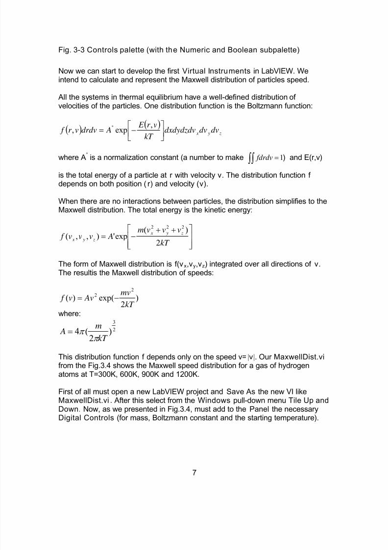
This distribution function f depends only on the speed v= |v |. Our MaxwellDist.vi from the Fig.3.4 shows the Maxwell speed distribution for a gas of hydrogenatoms at T=300K, 600K, 900K and 1200K.

First of all must open a new LabVIEW project and Save As the new VI likeMaxwellDist.vi . After this select from the Windows pull-down menu Tile Up andDown. Now, as we presented in Fig.3.4, must add to the Panel the necessaryDigital Controls (for mass, Boltzmann constant and the starting temperature).

7



In the control panel its necessary to put also two Waveform Graph selectingControls>Graph>Waveform Graph . With this operations finished we have allthe necessary controls and indicators in the panel.Now must change to the Diagram and we select two For Loop and oneFormula Node from Functions > Structures > For Loop and Functions >

Structures > Formula Node.One For Loop its necessary to compute the speed distribution and second oneto be able to compute de speed distribution for different temperatures. In theFormula node we introduce all the necessary constants and we compute thespeed distribution and energy. To add the necessary entries and outputs for theFormula Node we can click on his icon with the right taste of the mouse andselect Add Input or Add Output . All the necessary information connected withthe writing of formulas can be automatically vizualizated if the Show ContextHelp was activated (from Help > Show Context Help ).

To calculate the value of the N in the internal For Loop we used the numericicons from the subpalette Numeric of the Functions palette (Fig.3.5). This valueof N its connected with the range of the maximum particles speed V0 (we usedN=3 V 0) calculated for all the selected temperatures T=300K, 600K, 900K and1200K.

Fig. 3-4 The MaxwellDist.vi present particle speed d istr ibution and energy

8



Fig. 3-5 The Numeric subpalette and the N calculus

4. Data Acquisit ion with LabJack

In the last years a great number of companies designed and seal on the Data Acquisition market a high number of DAQ cards with a great variability in the ratioPRICE/QUALITY. We selected LabJack (Annex I.) for our laboratory applicationsbecause satisfy us with one of the best ratio price/quality but have also moreothers qualities:

Its an external card, easy to manipulate in laboratory

Easy and reliable hot USB connectivity Have an excellent connection interface Has a watchdog timer function available High quality of AD, DA conversion resolution Good low noise precision PGA amplifier to provide gains up to 20 Have a good compensated tension reference One frequency counter up to 1MHz LabVIEW drivers, applications and SDK included in price Flexible programming facilities

In the distribution package you will receive the LabJack card, USB connection

cable, a small documentation and a CD with all the necessary files. To be able touse the LabJack DAQ card for the first time it’s very easy.

With the PC on and using the included cable, connect the LabJack U12 to theUSB port on the PC or USB hub. The USB cable provides power andcommunication for the LabJack U12. The status LED should immediately blink 4times (at about 4 Hz), and then stay off while the LabJack enumerates.

9



Enumeration is the process where the PC’s operating system gathers informationfrom a USB device that describes it and it’s capabilities. The low-level drivers forthe LabJack U12 come with Windows and enumeration will proceedautomatically. The first time a device is enumerated on a particular PC, it cantake a minute or two, and Windows might prompt you about installing drivers.

Accept all the defaults at the Windows prompts, and reboot the PC if asked to doso. The Windows Installation CD might also be needed at this point. Make sure aCD with the correct version of Windows is provided. Enumeration occurswhenever the USB cable is connected, and only takes a few seconds after thefirst time.

When enumeration is complete, the LED will blink twice and remain on. Thismeans Windows has enumerated the LabJack properly.

If the LabJack fails to enumerate: Make sure you are running Windows OS version 4.10.2222 or higher, Try connecting the LabJack to another PC,

Try connecting a different USB device to the PC, Check our online forum and/or contact LabJack. When the LabJack installation is finished, it will start the National

Instruments LabVIEW Run-Time Engine (LVRTE) setup. The LVRTE is requiredfor the example applications: LJconfig, LJlogger, LJscope, and LJtest. Ifprompted to reboot after this installation, go ahead and do so.

Virus scanners can often interfere with the installation of the LVRTE. If you havetrouble running the example applications, repeat the LabJack softwareinstallation to make sure the LVRTE is installed.In the case of manual installation and CD browsing, we can find two maindirectories:

Imageo docso driverso exampleso and executable applications (LJconfig, LJcounter, LJfg,

LJlogger, LJscope, LJstream, LJtest) LabVIEW

o with the LabVIEW virtual instruments library Ljackuw.llb

After the initial software installation it’s good to test LabJack card with the help ofthe executable software’s (LJconfig, LJcounter, LJfg, LJlogger, LJscope,LJstream, LJtest). For this can execute the LJtest and LJconfig applications. InFig.4.1 you can see the LabVIEW interface in the case of one LabJack unitconnected to the USB port of our PC and was run LJtest.

10



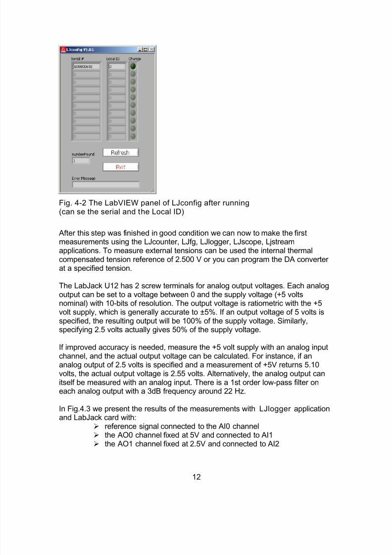
If you need to use more like one LabJack unit connected to the PC, you can usethe LJconfig application to see the serial of the cards and to change the LocalID.

In the Fig.4.2 you can se the panel of the application LJconfig and you canobserve the serial and the Local ID of one LabJack card who was connected atthe test moment. In this case we connected a LabJack card with the Serialnumber 100000692 and the card received the Local ID 0 (was detected onlyone card in the system).

Fig. 4-1 The LabVIEW panel of LJtest after f irst test running

11



Fig. 4-2 The LabVIEW panel of LJconfig after running(can se the serial and the Local ID)

After this step was finished in good condition we can now to make the firstmeasurements using the LJcounter, LJfg, LJlogger, LJscope, Ljstreamapplications. To measure external tensions can be used the internal thermalcompensated tension reference of 2.500 V or you can program the DA converterat a specified tension.

The LabJack U12 has 2 screw terminals for analog output voltages. Each analogoutput can be set to a voltage between 0 and the supply voltage (+5 voltsnominal) with 10-bits of resolution. The output voltage is ratiometric with the +5volt supply, which is generally accurate to ±5%. If an output voltage of 5 volts isspecified, the resulting output will be 100% of the supply voltage. Similarly,specifying 2.5 volts actually gives 50% of the supply voltage.

If improved accuracy is needed, measure the +5 volt supply with an analog inputchannel, and the actual output voltage can be calculated. For instance, if ananalog output of 2.5 volts is specified and a measurement of +5V returns 5.10volts, the actual output voltage is 2.55 volts. Alternatively, the analog output canitself be measured with an analog input. There is a 1st order low-pass filter oneach analog output with a 3dB frequency around 22 Hz.

In Fig.4.3 we present the results of the measurements with LJlogger applicationand LabJack card with:

reference signal connected to the AI0 channel the AO0 channel fixed at 5V and connected to AI1 the AO1 channel fixed at 2.5V and connected to AI2

12



Fig. 4-3 Measurements us ing LJlogger application

The external features of the LabJack U12 are: USB connector, DB25 digital I/O connector Status LED, 30 screw terminals.

The USB connection provides power and communication. No external powersupply is needed. The +5 volt connections available at various locations areoutputs; do not connect a power supply.

Figure 4.4 shows the top surface of the LabJack U12. Not shown the USB andDB25 connector, which are both on the top edge. The DB25 connector providesconnections for 16 digital I/O lines, called D0-D15. It also has connections forground and +5 volts. All connections besides D0-D15, are provided by the 30screw terminals shown in Figure 12. Each individual screw terminal has a label,

AI0 through STB.

The status LED blinks 4 times at power-up, and then blinks once and stays onafter enumeration (recognition of the LabJack U12 by the PC operating system).The LED also blinks during burst and stream operations, unless disabled. TheLED can be enabled/disabled through software using the functions AISample,

AIBurst, or AIStreamStart. Since the LED uses 4-5 mA of current, some usersmight wish to disable it for power-sensitive applications (can do this as you cansee in Fig.4.3 with LED on or off function).

13



Fig. 4-4 Top surface of the LabJack U12.

With the LabJack and LabVIEW software installed on your PC you can now usethe specific LabJack icons to write any new applications using LabVIEW VirtualInstruments. The LabJack palette of 21 icons (LJAI, LJAO, Bits to volt, Volts tobits, LJcount, LJDIO, LJreset…) inserted in the standard palette of LabVIEW youcan see now on the Fig.4.5.

14



Fig. 4-5 LabJack palette of icons in LabVIEW

We selected only 2 of the icons from 21, the LJAI and LJAO, to be introduced inFig.4.6 together with the minimal help for connection in LabVIEW applications.We can use now these icons to easy build specific applications for the laboratory.

Fig. 4-6 LabJack icons and LabVIEW help

In the Fig. 4.7 we used the LJAI and LJAO to build a virtual instrument namedGenRead.vi who generate 2 voltages and this voltages can be read on Cannel 1and Channel 2 voltmeters. Like in Fig. 4.3 the reference signal was connected tothe AI0 channel and the AO0 channel fixed at 3V was connected to AI1 and the

AO1 channel fixed at 4V and connected to AI2.

Fig. 4-7 Applications in LabVIEW using LJAI and LJAO

Now relatively easy can build laboratory applications that involve control ormeasure currents and tensions. To adapt the signals can use the facilities offeredby the LabJack card.

15



The LabJack U12 has 8 screw terminals for analog input signals. These can beconfigured individually and on-the-fly as 8 single-ended channels, 4 differentialchannels, or combinations in between. Each input has a 12-bit resolution and aninput bias current of ±90 μ A.

Input configuration: Single-Ended: The input range for a single-ended measurement is ±10 volts. Differential channels can make use of the low noise precision PGA to provide

gains up to 20, giving an effective resolution greater than 16-bits.

In differential mode, the voltage of each AI with respect to ground must bebetween ±10 volts, but the range of voltage difference between the 2 AI is afunction of gain (G) as follows:

G=1 ±20 voltsG=2 ±10 voltsG=4 ±5 volts

G=5 ±4 voltsG=8 ±2.5 voltsG=10 ±2 voltsG=16 ±1.25 voltsG=20 ±1 volt

The reason the range is ±20 volts at G=1 is that, for example, AI0 could be +10volts and AI1 could be -10 volts giving a difference of +20 volts, or AI0 could be -10 volts and AI1 could be +10 volts giving a difference of -20 volts.

For some experiments you can use also the DIO lines. Connections to 4 of theLabJack’s 20 digital I/O are made at the screw terminals, and are referred to as

IO0-IO3. Each pin can individually be set to input, output high, or output low.These 4 channels include a 1.5 k . series resistor that provides overvoltage/short-circuit protection. Each channel also has a 10 M resistor connected to ground.One common use of a digital input is for measuring the state of a switch. If theswitch is open, IO0 reads FALSE. If the switch is closed, IO0 reads TRUE.

While providing overvoltage/short-circuit protection, the 1.5 k . series resistor oneach IO pin also limits the output current capability. For instance, with an outputcurrent of 1 mA, the series resistor will drop 1.5 volts, resulting in an outputvoltage of about 3.5 volts.

Connections to 16 of the LabJack’s 20 digital I/O are made at the DB25connector, and are referred to as D0-D15. These 16 lines have noovervoltage/short-circuit protection, and can sink or source up to 25 mA each(total sink or source current of 200 mA max for all 16). This allows the D pins tobe used to directly control some relays. All digital I/O are CMOS output and TTLinput except for D13-D15, which are Schmitt trigger input. Each D pin has a 10M. resistor connected to ground.

16



5. Laborator ies using LabVIEW

Using this combination of LabVIEW software and LabJack card it’s easy todevelop a great variety of teaching and laboratory applications.

Laboratories, which are found in all engineering and science programs, are anessential part of the education experience. Not only do laboratories demonstratecourse concepts and ideas, but they also bring the course theory alive sostudents can see how unexpected events and natural phenomena affect real-world measurements and control algorithms. However, equipping a laboratory isa major expense and its maintenance can be difficult. Teaching assistants arerequired to set up the laboratory, instruct in the laboratory, and grade laboratoryreports. These time-consuming and costly tasks result in relatively low laboratoryequipment usage, especially considering that laboratories are available onlywhen equipment and teaching assistants are both available.

What if some of the basic laboratory experiments could be made available 24hours a day, seven days a week? What if students could have access toexperiments from their home or student dormitories? What if a professor wantedhis students to take a closer look at a classroom demonstration? What if aprofessor wanted to make a research demonstration available to students andothers at irregular times? What if a professor deriving a complex equation forsome application wanted his students to try different sets of parameters to bringout the essence of the model? What if a professor wanted his students to see anelectronic circuit in action, and even give them control of the operatingparameters?

All of these and many more exciting applications are now easily achievable withthe new technology available with National Instruments LabVIEW RemotePanels. With this standard feature of LabVIEW, a user can quickly andeffortlessly publish the front panel of a LabVIEW program for use in a standardWeb browser. Once published, anyone on the Web with the proper permissionscan access and control the experiment from the local server. If the LabVIEWprogram controls a real-world experiment, demonstration, calculation, etc.,LabVIEW Remote Panels turns the application into a remote laboratory with noadditional programming or development time.

A remote laboratory (Fig.5.1) is defined as a computer-controlled laboratory that

can be accessed and controlled externally over some communication medium.For this discussion, a remote laboratory is an experiment, demonstration, orprocess running locally on a LabVIEW platform but with the ability to bemonitored and controlled over the Internet from within a Web browser. In thesimplest case, the remote laboratory server can be an experiment connected to acomputer through a standard interface (DAQ, GPIB, serial, parallel, etc) and withthe host computer connected to the Internet. The client can be any computerconnected to the Internet running a simple browser. Once connected, the client

17



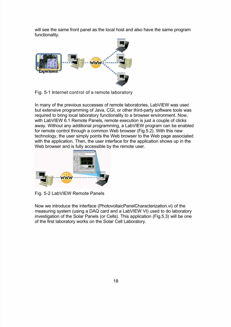
will see the same front panel as the local host and also have the same programfunctionality.

Fig. 5-1 Internet cont rol of a remote laboratory

In many of the previous successes of remote laboratories, LabVIEW was usedbut extensive programming of Java, CGI, or other third-party software tools wasrequired to bring local laboratory functionality to a browser environment. Now,with LabVIEW 6.1 Remote Panels, remote execution is just a couple of clicksaway. Without any additional programming, a LabVIEW program can be enabledfor remote control through a common Web browser (Fig.5.2). With this newtechnology, the user simply points the Web browser to the Web page associatedwith the application. Then, the user interface for the application shows up in theWeb browser and is fully accessible by the remote user.

Fig. 5-2 LabVIEW Remote Panels

Now we introduce the interface (PhotovoltaicPanelCharacterization.vi) of themeasuring system (using a DAQ card and a LabVIEW VI) used to do laboratoryinvestigation of the Solar Panels (or Cells). This application (Fig.5.3) will be oneof the first laboratory works on the Solar Cell Laboratory.

18



Fig. 5-3 The Panel and Diagram of the

PhotovoltaicPanelCharacterization.VI

Now we can use this Virtual Instrument to present how easy we can buildRemote Panels using the LabVIEW facilities. In the Fig. 5.4 we present thisVirtual Instrument web remote controlled with LabVIEW.

Fig. 5-4 Web control of the PhotovoltaicPanelCharacterization.VI

To build this application, you must use the LabVIEW (from version 6.1 to the lastone) and make some simple steps. First of all must open the application. Afterthis select Tools > web Publishing Tool… and you open a simple interface(Fig.5.5) when you can introduce some informations (Text 1 and Text 2) aboutyour application and after that: must Start Web Server and Preview in Browser .If you are satisfied you must close all with Save to Disk (an put the PhotovoltaicPanel Characterization.htm in www directory of LabVIEW).

19



Fig. 5-5 Web Publish ing in LabVIEW

In the Annex 2 we present now some Virtual Instruments with the Panels andDiagrams and a short description. This applications was build to proof thecapability of LabVIEW software to be a flexible tool to develop: teaching support,laboratory applications and also sophisticated research virtual instruments.

The creation of same virtual instruments gives the possibility to produce somerather cheap research environments of high quality, with a friendly interface and

an easy maintenance. Also, virtual labs and virtual instrumentation can sustain very well the theoreticalcourses from the perspective of both practical and research work parts.

The appearance of some software as LabVIEW, that don’t request very strongprogramming knowledge in order to create some complex applications, gives aidat the creation of virtual labs and virtual instrumentation

6. References 1. P. Cotfas, D. Ursutiu, D. Cotfas, C. Samoila “Implementarea Metodei

Entropiei Maxime in LabVIEW” RIV Anul III, Vol. III, Nr 3(11), toamna 2000,ISSN 1453-8059;

2. D. Ursutiu “Initiere in LabVIEW Programarea grafica in fizica si electronica ”,Editura Lux Libris, Brasov, 2001;

3. P. Cotfas, D. Ursutiu, C. Samoila “Using LabVIEW in Computer BasedLearning”, “Interactive Computer aided Learning Tools and Applications“ Ed.M.Auer and U. Ressler, ICL99 Workshop, ISBN 3-7068-0755-6;

20



4. P. Cotfas, D. Ursutiu, C. Samoila “Creating a Virtual Lab using LabVIEW”International Conf. TICE 2000, 18-20.10.2000, Troyes, France;

5. P. Cotfas, D. Ursutiu, C. Samoila “Virtual Laboratory and VirtualInstrumentation” ,“Internet as a Vehicle for Teaching“, Ed. Susan English,Mihai Jalobeanu, Nicolaie Nistor, Romanian Internet Learning Workshop

“RILW2001“, august 11-20 2001, ISBN 973-85023-7-36. http://www.labjack.com/support.html LabJack company documentation7. http://www.ni.com National Instruments company documentation8. Cotfas,P., Ursutiu, D., Cotfas D., Samoila C. “Implementarea Metodei

Entropiei Maxime in LabVIEW” RIV Anul III, Vol. III, Nr 3(11), toamna 2000,ISSN 1453-8059

9. Egarievwe, S.U., Adepeju, A., Gautam, B., Oseoghaghare, K.O., La Keisha A.F., Shean. K.T.,Eugene C.W. Internet Application of LabVIEW In ComputerBased, EURODL 2000

http://www.labjack.com/support.html

http://www.ni.com/

http://www.ni.com/

http://www.labjack.com/support.html

1 Introduction in LabVIEW

Documents

Transcript of 1 Introduction in LabVIEW