Solving Parallel Machine Scheduling Problems by

Column Generation

Zhi-Long ChenDepartment of Systems Engineering

University of PennsylvaniaPhiladelphia, PA 19104-6315

Warren B. PowellDepartment of Civil Engineering & Operations Research

Princeton UniversityPrinceton, NJ 08544, USA

July 1996(Revised April 1997, January 1998)

Abstract

We consider a class of problems of scheduling n jobs on m identical, uniform, or unre-lated parallel machines with an objective of minimizing an additive criterion. We proposea decomposition approach for solving these problems exactly. The decomposition ap-proach �rst formulates these problems as an integer program, and then reformulatesthe integer program, using Dantzig-Wolfe decomposition, as a set partitioning problem.Based on this set partitioning formulation, branch and bound exact solution algorithmscan be designed for these problems. In such a branch and bound tree, each node is thelinear relaxation problem of a set partitioning problem. This linear relaxation problemis solved by a column generation approach where each column represents a scheduleon one machine and is generated by solving a single machine subproblem. Branchingis conducted on variables in the original integer programming formulation instead ofvariables in the set partitioning formulation such that single machine subproblems aremore tractable. We apply this decomposition approach to two particular problems: thetotal weighted completion time problem and the weighted number of tardy jobs problem.The computational results indicate that the decomposition approach is promising andcapable of solving large problems.

Key words: Parallel machine scheduling; Set partitioning; Dantzig-Wolfe decompo-sition; Column generation; Branch and bound

1 Introduction

We consider a class of problems of scheduling n independent jobs N = f1; 2; :::; ng on

m identical, uniform, or unrelated parallel machinesM = f1; 2; :::;mg with an objective

of minimizing an additive criterion. For ease of presentation, we denote this class of

problems as PMAC. In the PMAC problems, each job i 2 N has m processing times pij

(j 2M), a weight wi, a due date di, and probably other problem dependent parameters.

Here pij is the actual processing time of job i if it is processed on machine j. As a

convention, processing times pij , for all i 2 N; j 2 M , satisfy the following properties.

In the case of identical machines, all the machines have the same speed and hence

processing times of a job are identical on di�erent machines, i.e. pij � pi. In the case of

uniform machines, machines may have di�erent speeds and processing times of a job may

di�er by speed factors, i.e. pij = pi=sj , where sj re ects the speed of machine j. Finally,

in the case of unrelated machines, pij is arbitrary and has no special characteristics.

We are interested in classical settings, that is, all the parameters are deterministic; all

the jobs are available for processing at time zero; and no preemption is allowed during

processing.

Let Cj denote the completion time of job j in a schedule. Then a general additive

criterion can be denoted asXj2N

fj(Cj), where fj(�) is a real-valued function. Using

the commonly accepted three �eld classi�cation terminology for machine scheduling

problems (see, e.g. Lawler, Lenstra, Rinnooy Kan and Shmoys [22]), we denote the

general PMAC problem by P jjPfj(Cj) for the identical machine case, Qjj

Pfj(Cj) for

the uniformmachine case, andRjjPfj(Cj) for the unrelated machine case. In this paper,

we mainly focus on the following two particular problems: the total weighted completion

time problem, denoted as P jjPwjCj, Qjj

PwjCj, or Rjj

PwjCj, respectively for the

identical, uniform, or unrelated machine case; and the weighted number of tardy jobs

problem, denoted similarly as P jjPwjUj , Qjj

PwjUj , or Rjj

PwjUj, where Uj = 1 if

job j is late, i.e. Cj > dj , and 0 otherwise.

Needless to say, the PMAC problems are fundamental to numerous complex real-

1

world applications. They are widely noted in survey papers (e.g. Cheng and Sin [9], and

Lawler, Lenstra, Rinnooy Kan and Shmoys [22]) and books (e.g. Baker [1], and Pinedo

[26]). Unfortunately, most of them, including P jjPwjCj, the easiest case of the total

weighted completion time problem, and P jjPwjUj, the easiest case of the weighted

number of tardy jobs problem, are NP-hard, and very few exact solution algorithms

can be found in the literature. As noted in Lawler, Lenstra, Rinnooy Kan and Shmoys

[22], the dynamic programming techniques of Rothkopf [27] and Lawler and Moore [23]

can solve some of these problems, including the total weighted completion time problem

and the weighted number of tardy jobs problem, in which it is possible to schedule

jobs on a single machine in a predetermined order. However, it is impractical to solve

even very small sized problems using these algorithms which require prohibitively high

order of time: O(mminf3n; n2ng) for P jjPfj(Cj); O(mnCm�1) for Qjj

PwjCj; and

O(mnCm) for RjjPwjCj, Qjj

PwjUj , and Rjj

PwjUj , where C is an upper bound on

the completion time of any job in an optimal schedule. To the best of our knowledge,

there is no other exact solution algorithms in the literature for the problems: QjjPwjCj,

RjjPwjCj, P jj

PwjUj , Qjj

PwjUj , and Rjj

PwjUj.

For the problem P jjPwjCj, however, besides this possible dynamic programming

algorithm, there are lower bounding techniques in the literature that can be used to

design branch and bound algorithms. Eastman, Even and Isaccs [13] give a lower bound

for the optimal objective function. This lower bound has been the basis for the branch

and bound algorithms of Elmaghraby and Park [14], Barnes and Brennan [2], and Sarin,

Ahn and Bishop [28]. Recently, Webster [33, 34, 35] gives tighter lower bounds based

on the idea of considering a job as a collection of subjobs linked together by a group

constraint. However, there is no branch and bound algorithm reported in the litera-

ture using Webster's lower bounds. Belouadah and Potts [4] formulate the problem

P jjPwjCj as an integer program and use the well-known Lagrangian relaxation lower

bounding scheme to design a branch and bound algorithm which is capable of solving

instances with up to 3 machines and 30 jobs within a reasonable time.

Since we mainly focus on the total weighted completion time problem and the

2

weighted number of tardy jobs problem, we only give a brief review of algorithms for

other PMAC problems. Barnes and Brennan [2] propose a branch and bound exact

solution algorithm for the total tardiness problem in the identical machine case. Not

surprisingly, their algorithm can only solve problems with up to 20 jobs and 4 identical

machines. Besides this, De, Ghosh and Wells [11] give an O(nm[w(n=m+1)]2m) dynamic

programming exact solution algorithm for a problem involving earliness, tardiness and

due date penalties. Obviously, this DP algorithm is only capable of solving problems

with a small number of machines and jobs. For possible algorithms for special cases of

the PMAC problems, the reader is referred to the survey papers: Cheng and Sin [9], and

Lawler, Lenstra, Rinnooy Kan and Shmoys [22].

In this paper, we propose a decomposition approach for solving the PMAC problems

exactly. The decomposition approach �rst formulates these problems as an integer pro-

gram, and then reformulates the integer program, using Dantzig-Wolfe decomposition,

as a set partitioning problem. Based on this set partitioning formulation, branch and

bound exact solution algorithms can be designed for the PMAC problems. In such a

branch and bound tree, each node is the linear relaxation problem of a set partitioning

problem. This linear relaxation problem is solved by a column generation approach

where each column represents a schedule on one machine and is generated by solving a

single machine subproblem. Branching is conducted on variables in the original integer

programming formulation instead of variables in the set partitioning problem such that

the resulting subproblems are more tractable.

We apply this decomposition approach to the two particular problems: the total

weighted completion time problem and the weighted number of tardy jobs problem.

The computational results indicate that the decomposition approach is promising and

capable of solving large problems.

The success of our decomposition approach is mainly due to the excellent lower

bounding obtained from the linear relaxation of the set partitioning problem. We will

see later that in the case of the total weighted completion time problem, for each problem

size tested, the average deviation (based on twenty test problems) of the linear relaxation

3

solution value from the integer solution value is always within 0:1%; and in the case of

the weighted number of tardy jobs problem, this average deviation is always within

0:8%. Due to extremely tight lower bounds, very few branch and bound nodes need to

be explored in the corresponding branch and bound algorithms.

We note that at the same time when we were conducting this research, van den

Akker, Hoogeveen and van de Velde [30] independently suggested a similar approach to

the PMAC problems. However, the branching strategy used by them is di�erent from

that used by us. Their branching is based on the completion times of jobs appearing in

a fractional solution, while ours is based on the ordering relations of jobs. They applied

the approach to the problem P jjPwjCj and showed its e�ectiveness. Quite interest-

ingly, also at the same time, Chan, Kaminsky, Muriel and Simchi-Levi [7] independently

proposed and analyzed the column generation approach to the set partitioning formu-

lation of the problem P jjPwjCj. Their emphasis is on worst-case and probabilistic

analysis. They proved in theory that the worst-case deviation of the linear relaxation

solution value from the integer solution value is no more thanp2�12 � 100%.

This paper is organized as follows. The decomposition approach is described for the

general PMAC problem in the next section. Then in Sections 3 and 4, this approach

is applied, respectively, to the total weighted completion time problem (P jjPwjCj,

QjjPwjCj, and Rjj

PwjCj) and to the weighted number of tardy jobs problem (P jj

PwjUj,

QjjPwjUj, and Rjj

PwjUj). The resulting single machine subproblems are NP -hard

and solved by pseudo-polynomial dynamic programming algorithms. In Section 5, com-

putational experiments are conducted and their results are reported. Finally, in Section

6, we conclude the paper.

2 Decomposition Approach for the PMAC Prob-

lems

In this section, we describe in detail the decomposition approach for the PMAC prob-

lems. First, in Section 2.1, we give a general integer programming formulation for the

4

problems. Then, in Section 2.2, we decompose this formulation, using Dantzig-Wolfe de-

composition, into a set partitioning master problem and m single machine subproblems.

Then the linear relaxation of the set partitioning problem is solved by a column genera-

tion procedure. Finally, in Section 2.3, a branch and bound exact solution algorithm is

brie y described.

We note that the decomposition approach is applicable, directly or indirectly, to

virtually every individual PMAC problem. However, the e�ciency of the approach

mainly depends on whether single machine subproblems resulted from the decomposition

can be solved e�ciently. The formulations we are going to give (e.g. IP1 and IP2 of

Section 2.1, and SP1 and SP2 of Section 2.2) only serve as a representative for numerous

PMAC problems. When a particular PMAC problem is concerned, we may not directly

apply these general formulations to the problem; instead, it may be necessary to modify

these formulations appropriately so that more e�cient algorithms for the problem can

be designed. As we will see later, for the total weighted completion time problem, we

directly apply these formulations, while for the weighted number of tardy jobs problem,

we slightly modify these formulations.

2.1 Integer Programming Formulation

First de�ne a partial schedule on a single machine to be a schedule formed by a subset of

jobs of N on that machine. Clearly, a schedule for a PMAC problem (where m machines

are involved) consists of m partial schedules, one for each machine.

For a given PMAC problem, there may exist a predetermined job ordering restriction

which speci�es, for each job i, a set of jobs that must be scheduled before or after

job i. The job ordering restriction in a problem could be given both externally by

the problem itself (e.g. precedence constraints for jobs imposed by the problem) and

internally by optimality properties (e.g. some ordering patterns an optimal schedule

must follow). Note that, in the branch and bound algorithm described later, each

branch and bound node is a PMAC problem with an additional constraint imposed by

5

the branching rule which enforces some jobs to be scheduled before or after some other

jobs. The job ordering restriction in the problem corresponding to each branch and

bound node includes the job ordering constraint imposed by the branching rule as well.

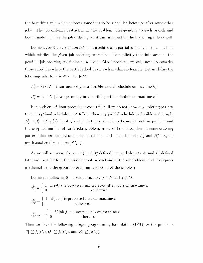
De�ne a feasible partial schedule on a machine as a partial schedule on that machine

which satis�es the given job ordering restriction. To explicitly take into account the

possible job ordering restriction in a given PMAC problem, we only need to consider

those schedules where the partial schedule on each machine is feasible. Let us de�ne the

following sets, for j 2 N and k 2M :

Akj = fi 2 N j i can succeed j in a feasible partial schedule on machine kg

Bkj = fi 2 N j i can precede j in a feasible partial schedule on machine kg

In a problem without precedence constraints, if we do not know any ordering pattern

that an optimal schedule must follow, then any partial schedule is feasible and simply

Akj = Bk

j = N n fjg for all j and k. In the total weighted completion time problem and

the weighted number of tardy jobs problem, as we will see later, there is some ordering

pattern that an optimal schedule must follow and hence the sets Akj and Bk

j may be

much smaller than the set N n fjg.

As we will see soon, the sets Akj and B

kj de�ned here and the sets Aj and Bj de�ned

later are used, both in the master problem level and in the subproblem level, to express

mathematically the given job ordering restriction of the problem.

De�ne the following 0 � 1 variables, for i; j 2 N and k 2M :

xkij =

(1 if job j is processed immediately after job i on machine k0 otherwise

xk0j =

(1 if job j is processed �rst on machine k0 otherwise

xkj;n+1 =

(1 if job j is processed last on machine k0 otherwise

Then we have the following integer programming formulation (IP1) for the problems

P jjPfj(Cj), Qjj

Pfj(Cj), and Rjj

Pfj(Cj).

6

IP1:

minXj2N

fj(Cj) (1)

subject to

Xk2M

Xi2Bk

j[f0g

xkij = 1; 8j 2 N (2)

Xj2N

xk0j � 1; 8k 2 M (3)

Xi2Bk

j[f0gxkij =

Xi2Ak

j[fn+1gxkji; 8j 2 N; k 2M (4)

Cj =Xk2M

0B@pjkxk0j + X

i2Bkj

(Ci + pjk)xkij

1CA ; 8j 2 N (5)

xkij 2 f0; 1g; 8i; j 2 N; k 2M (6)

The objective function (1) seeks to minimize a given additive criterion. Constraints

(2) and (3) ensure that each job is processed exactly once and each machine is uti-

lized at most once, respectively. Constraint (4) guarantees that the assignment of jobs

to machines is well-de�ned. This constraint plays the same role as ow conservation

constraints in many network ow problems. Constraint (5) de�nes completion time

Cj. The last constraint (6) represents binary integrality requirement of 0 � 1 variables.

Constraints (4), (5) and (6) ensure that the partial schedule on each machine is feasible.

For the problem P jjPfj(Cj), since all the machines are identical, we do not need

to distinguish di�erent machines, and hence the formulation (1)-(6) can be simpli�ed.

De�ne sets Aj and Bj and variables xij; x0j; xj;n+1 similarly to Akj , B

kj , x

kij; x

k0j; x

kj;n+1,

respectively, as follows:

Aj = fi 2 N j i can succeed j in a feasible partial schedule on a single machineg

Bj = fi 2 N j i can precede j in a feasible partial schedule on a single machineg

xij =

(1 if job i is processed immediately before job j on some machine0 otherwise

x0j =

(1 if job j is processed �rst on some machine0 otherwise

7

xj;n+1 =

(1 if job j is processed last on some machine0 otherwise

Then the simpli�ed integer programming formulation (IP2) for the problem P jjPfj(Cj)

is

IP2:

minXj2N

fj(Cj) (7)

subject to

Xi2Bj[f0g

xij = 1; 8j 2 N (8)

Xj2N

x0j � m (9)

Xi2Bj[f0g

xij =X

i2Aj[fn+1gxji; 8j 2 N (10)

Cj = pjx0j +Xi2Bj

(Ci + pj)xij; 8j 2 N (11)

xij 2 f0; 1g; 8i; j 2 N (12)

where constraints (9) represent that there are at most m machines available. The other

constraints have similar meanings to those in the preceding formulation IP1.

2.2 Dantzig-Wolfe Decomposition

In this subsection, we decompose the integer programming formulations IP1 and IP2

given in Section 2.1 into a master problem with a set partitioning formulation (Section

2.2.1) and some single machine subproblems (Section 2.2.3). We then use the column

generation approach to solve the linear relaxation of the set partitioning formulation

(Section 2.2.2).

2.2.1 The Set Partitioning Master Problem

Applying Dantzig-Wolfe decomposition [10], we decompose the formulation IP1 into

a master problem consisting of (1), (2), and (3), and m subproblems with feasible re-

gions de�ned by (4), (5), and (6). It is easy to see that, for any �xed k, any point

8

�xkij : i; j 2 N

�in the feasible region of the k-th subproblem, that is, the region given by

constraints (4) and (6) with the �xed k, together with Cj's de�ned in (5), corresponds

to a feasible partial schedule on machine k. We will see in Section 2.2.3 that each of the

m subproblems is a single machine scheduling problem.

Let k denote the set of all feasible partial schedules on machine k. Let fks be the

total cost of schedule s 2 k. For each job j 2 N , let akjs = 1 if schedule s 2 k covers

job j, and 0 otherwise. De�ne 0� 1 variables, for k 2M and s 2 k:

yks =

(1 if schedule s 2 k is used0 otherwise

Then the master problem can be formulated as the following set partitioning problem

(SP1).

SP1:

minXk2M

Xs2k

fks yks (13)

subject to

Xk2M

Xs2k

akjsyks = 1; 8j 2 N (14)

Xs2k

yks � 1; 8k 2M (15)

yks 2 f0; 1g; 8s 2 k; k 2M (16)

Constraints (14) and (15) correspond to the original constraints (2) and (3) and mean

that each job is covered by exactly one feasible partial schedule and each machine is

occupied by at most one feasible partial schedule, respectively.

For the problem P jjPfj(Cj), this master problem can be simpli�ed, if we apply

Dantzig-Wolfe decomposition to the formulation IP2. Let denote the set of all feasible

partial schedules on a single machine. For any s 2 , de�ne fs and ajs similarly to fks

and akjs respectively. De�ne variable ys = 1 if schedule s 2 is used and 0 otherwise.

Then the set partitioning master problem (SP2) for the problem P jjPwjCj is

SP2:

minXs2

fsys (17)

9

subject to

Xs2

ajsys = 1; 8j 2 N (18)

Xs2

ys � m (19)

ys 2 f0; 1g; 8s 2 (20)

where constraint (18) has the same meaning as (14) in SP1 and constraint (19) is

equivalent to (9) in IP2.

Since, the formulations SP1 and IP1 (SP2 and IP2) are both valid formulations for

the same general PMAC problem, the solution value of the formulation SP1 (SP2) must

be equal to that of the formulation IP1 (IP2), respectively. But, SP1 and SP2 are

not merely reformulations of IP1 and IP2. The di�erence lies in their linear relaxation

problems. Relaxing the integrality constraints (6), (12), (16) and (20), we get the

linear relaxation problems, denoted by LIP1, LIP2, LSP1 and LSP2, respectively

corresponding to the integer problems IP1, IP2, SP1 and SP2. The solution value

of LSP1 is usually greater than that of LIP1 because the set k is smaller than the

set of points (xkij : i; j 2 N) in the region given by (4) and the linear relaxation of (6).

The same relation is true for the formulations LSP2 and LIP2. This means that the

set partitioning formulations can yield tighter lower bounds than the original integer

programming formulations. Furthermore, the formulations LIP1 and LIP2 are not

linear programs and may not be easy to solve because they involve nonlinear constraints

(5) and (11), while the formulations LSP1 and LSP2 are linear programs and can

be solved easily using the column generation approach described later. Therefore, in

our branch and bound algorithm, we mainly work on the SP formulations SP1 and

SP2, instead of the original IP formulations IP1 and IP2. However, in the algorithm,

we branch on the variables in the IP formulations, instead of the variables in the SP

formulations, to make the subproblems more tractable.

10

2.2.2 Column Generation Procedure for Solving LSP1 and LSP2

As we mentioned earlier, each column in LSP1 and LSP2 represents a feasible partial

schedule on a single machine. As the number of feasible partial schedules on a machine,

i.e. jkj or jj, can be extremely large, it is impossible to explicitly list all the columns

when solving LSP1 and LSP2. So we use the column generation approach (see, e.g.

Lasdon [20]) to generate necessary columns only in order to solve LSP1 and LSP2

e�ciently.

Column generation approach has been successfully applied to many large scale opti-

mization problems, such as cutting stock (Gilmore and Gomory [16], Vance, Barnhart,

Johnson and Nemhauser [32]), vehicle routing (Desrochers, Desrosiers and Solomon [12]),

air crew scheduling (Lavoie, Minoux and Odier [21], Vance [31]), lot sizing and schedul-

ing (Cattrysse, Salomon, Kuik and Van Wassenhove [6]), and graph coloring (Mehrotra

and Trick [24]).

The column generation procedure consists of the following four major steps:

� solving a restricted master problem of LSP1 or LSP2, i.e, the problem LSP1

or LSP2 with a restricted number of columns;

� using the dual variable values of the solved restricted master problem to update

cost coe�cients of the subproblems;

� solving single machine subproblems; and

� getting new columns with negative reduced costs based on the subproblem solu-

tions and adding the new columns to the restricted master problem.

These steps are repeated until no column with negative reduced cost can be gener-

ated, upon which we will have solved the problem LSP1 or LSP2 to optimality.

The restricted master problem of LSP1 or LSP2 is a linear program which can

be e�ciently solved using a linear programming solver. The e�ciency of the column

generation procedure mainly depends on how fast a subproblem can be solved. Actually,

11

it is crucial to �nd an appropriate formulation (IP1, IP2, or their modi�ed version) for

a particular problem so that the resulting subproblems have desired structures and can

be solved e�ciently.

It is worth noting some implementation strategies that may be used in the column

generation algorithm. First, in order to have an initial feasible restricted master problem

of LSP1 or LSP2, we can either use a heuristic to generate a feasible schedule and use

the resulting m single machine schedules as the columns in the initial restricted master

problem, or slightly modify the formulation LSP1 or LSP2 by adding an arti�cial vari-

able to the left-hand side of each of the n equality constraints and a su�ciently large

linear function of each arti�cial variable to the objective function. Second, if more than

one columns with a negative reduced cost are available from the subproblem solution,

then it may be bene�cial to add multiple such columns, instead of only the column

with the most negative reduced cost, to the restricted master problem. Our computa-

tional experiments (described in Section 5) seem to indicate that the implementation

which adds �ve to ten columns (if available) in each iteration is more e�cient than the

implementation which adds only one column or adds more than twenty columns.

2.2.3 Single Machine Subproblems

The goal of solving subproblems is to �nd the column with the minimum reduced cost

to be added to the restricted master problem when solving LSP1 and LSP2. If the

minimum reduced cost is nonnegative, then we can terminate the column generation

procedure and the problem is solved. In the restricted master problem of LSP1, let

�j denote the dual variable value corresponding to job j, for each j 2 N , in constraint

(14), and �k denote the dual variable value corresponding to machine k, for each k 2M ,

in constraint (15). Then the reduced cost rks of the column corresponding to s 2 k is

given by:

rks = fks �Xj2N

akjs�j � �k (21)

12

Similarly, in the restricted master problem of LSP2, let �j denote the dual variable value

corresponding to job j, for each j 2 N , in constraint (18), and � denote that correspond-

ing to the constraint (19). Then the the reduced cost rs of the column corresponding to

s 2 is as follows:

rs = fs �Xj2N

ajs�j � � (22)

Hence, when solving LSP1, we need to solve m subproblems, one for each machine,

in order to �nd the column with the minimum reduced cost. The k-th subproblem is

to �nd a feasible partial schedule s 2 k on machine k such that its reduced cost rks is

minimized. By contrast, when solving LSP2, since all the machines are identical, we

only need to solve one subproblem which is to �nd a feasible partial schedule s 2 on

a single machine such that its reduced cost rs is minimized.

By the reduced cost formula (21) or (22), more precisely, a single machine subproblem

on some machine is to �nd a subset of jobs of N and a schedule for these jobs on that

machine which satis�es the job ordering restriction of the problem such that the total

cost of the jobs in the schedule (i.e. the quantity fks or fs) minus the total dual variable

value of these jobs (i.e. the quantityP

j2N akjs�j orP

j2N ajs�j) is minimized. Here the

dual variable values corresponding to the machine, i.e. �k and �, are ignored since they

are common to all the feasible partial schedules on that machine. We will see later that

single machine subproblems for the total weighted completion time problem and the

weighted number of tardy jobs problem are all ordinarily NP -hard and can be solved

by pseudopolynomial dynamic programming algorithms.

2.3 Branch and Bound Algorithm

In this section, we describe a branch and bound (b&b) exact solution algorithm for

the PMAC problems. Special attention is given to the branching strategy used in the

algorithm.

For solving the problems QjjPfj(Cj) and Rjj

Pfj(Cj), the b&b algorithm is based

on the formulations IP1, SP1, and their linear relaxations LIP1 and LSP1. While, for

13

solving the problem P jjPfj(Cj), the b&b algorithm uses the corresponding simpli�ed

formulations IP2, SP2, LIP2, and LSP2. In the b&b tree, each b&b node is a linear

relaxation problem LSP1 or LSP2 with some additional constraint imposed by the

branching rule (described later). These linear relaxation problems are solved by the

column generation procedure described earlier.

Usually, in a branch and bound algorithm, two classes of decisions need to be made

(see, e.g. Nemhauser and Wolsey [25]) throughout the algorithm. One is called node

selection, that is, to select an active node in the b&b tree to be explored (solved).

The other is called branching variable selection, that is, to select a fractional variable

to branch on. The node selection strategy we use in our algorithm combines the rule

depth-�rst-search (also known as last-in-�rst-out (LIFO)) and the rule best-lower-bound.

If the current b&b node is not pruned, then the depth-�rst-search rule is applied such

that one of the two son nodes of the current b&b node is selected as the next node to

be solved. If the current b&b node is pruned, then the best-lower-bound rule is applied

such that an active node in the b&b tree with the smallest lower bound is selected as

the next node to be explored.

For solving our problem SP1 (i.e. the problems QjjPfj(Cj) and Rjj

Pfj(Cj)) or

SP2 (i.e. the problem P jjPfj(Cj)), traditional branching on the y-variables in the

problem may cause trouble along a branch where a variable has been set to zero. Recall

that yks in SP1 (ys in SP2) represents a feasible partial schedule on some machine k

generated by solving a single machine subproblem. The branching yks = 0 (ys = 0) means

that this partial schedule is excluded and hence no such schedule can be generated in

subsequent subproblems on that machine. However, it is not an easy task to exclude a

schedule when solving a single machine subproblem.

Fortunately, there is a simple remedy to this di�culty. Instead of branching on the

y-variables in the set partitioning formulation SP1 (SP2), we branch on x-variables

in the original formulation IP1 (IP2). This branching variable selection strategy, that

is, branching on variables in the original formulation, has been proved successful in

many branch and bound algorithms for problems that can be reformulated, usually by

14

Dantzig-Wolfe decomposition, into a master problem and one or some subproblems. See

Barnhart, Johnson, Nemhauser, Savelsbergh, and Vance [3] for a class of such problems.

Observing the relation between the set partitioning formulation SP1 (SP2) and

the original formulation IP1 (IP2), we can see that for any feasible solution (yks ; s 2

k; k 2 M) to LSP1 ((ys; s 2 ) to LSP2), there is a corresponding feasible solution

(xkij; i; j 2 N; k 2 M) to the problem LIP1 ((xij; i; j 2 N) to the problem LIP2), such

that

xkij =Xs2k

esijyks (23)

and

xij =Xs2

esijys (24)

where esij is 1 if jobs i and j are both contained in schedule s and job j follows job i

immediately in s, and 0 otherwise.

Obviously, if the y-variable solution, i.e. (yks ; s 2 k; k 2 M) or (ys; s 2 ), is

integral, then the corresponding x-variable solution given by (23) and (24) is integral as

well. Actually, the reverse is also true. This is proved in Lemma A1 in the Appendix.

Once we have explored a b&b node (i.e. a problem LSP1 or LSP2), if the solution

(yks ; s 2 k; k 2 M) or (ys; s 2 ) is fractional and the integer part of its solution value

is less than the upper bound of the b&b tree, then the corresponding x-variable solution

is computed by (23) or (24). By Lemma A1, this x-variable solution must be fractional.

Based on this x-variable solution, an appropriate fractional x-variable is then selected

to branch on next. For ease of presentation, we distinguish the two problems: SP1 and

SP2, and describe the branching strategy for each of them separately in the following

paragraphs.

In the case of SP2, a pair of jobs (h; l) is selected such that xhl = arg minxij

fjxij � 0:5jg,

i.e. the pair (h; l) has the value xhl with the maximum integer infeasibility. Two son

nodes are then created, one along the branch with xhl �xed as 0 and the other along

the branch with xhl �xed as 1. If xhl is �xed as 0, then the initial restricted master

problem of the corresponding son node consists of all the columns of its father node

15

except the ones in which job l is scheduled immediately after job h if h 6= 0 or job l is

scheduled �rst on a machine if h = 0. At the same time, the job ordering restriction is

updated such that Bl := Bl n fhg, which guarantees that no schedule will be generated

where job l is processed immediately after job h if h 6= 0 or where job l is processed

�rst on a machine. If xhl is �xed as 1, then the initial restricted master problem of the

corresponding son node consists of all the columns of its father node except the ones

in which job l is scheduled immediately after a job other than h and the ones in which

a job other than l is scheduled immediately after job h. The job ordering restriction

is also updated accordingly such that Bl := fhg, which ensures that any schedule that

contains job l processes job h immediately before l.

In the case of SP1, the branching variable selection strategy is slightly di�erent from

the case of SP2. First de�ne

qij =Xk2M

xkij (25)

The branching variable selection consists of two stages. In the �rst stage, branching

is based on values of the variables qij. If some qij's are fractional, then select a pair

of jobs (h; l) with the value qhl having the maximum integer infeasibility, i.e. qhl =

arg minqijfjqij � 0:5jg. Two son nodes are created similarly as in the case of SP2. If qhl

is �xed as 0, then xkhl, for each k 2 M , is �xed as 0. If qhl is �xed as 1, then all xkil

with i 6= h, and xkhj with j 6= l are �xed as 0. In the son node with qhl �xed as 0, the

restricted master problem is constructed in the same way as the son node with xhl = 0

in the case of SP2. The job ordering restriction for this son node is updated as follows:

Bkl := Bk

l n fhg for each k 2 M . In the son node with qhl �xed as 1, the restricted

master problem is also constructed in the same way as the son node with xhl = 1 in the

case of SP2. The job ordering restriction is updated by letting: Bkl := Bk

l

Tfhg for each

k 2M .

When every qij is integral, it is possible for some xkij's to be fractional. In such a

case, we use the second stage branching strategy which selects a branching variable xvhl

such that xvhl = arg minxkij

fjxkij � 0:5jg. Similarly, two son nodes are created, one along

16

the branch with xvhl �xed as 0 and the other along the branch with xvhl �xed as 1. In

the �rst son node, the restricted master problem consists of all the columns of its father

node except the ones that schedule job l immediately after job h on machine v; and

the job ordering restriction is updated: Bvl = Bv

l n fhg. In the second son node, the

restricted master problem consists of all the columns of its father node except the ones

that contain at least one of the jobs h and l on a machine other than machine v and the

ones that schedule job l immediately after a job other than job h or schedule a job other

than h immediately before job l; and the job ordering restriction is updated as follows:

Bvl = fhg, and Bk

l = �;Bkj = Bk

j n fhg for k 2M n fvg; j 2 N n flg.

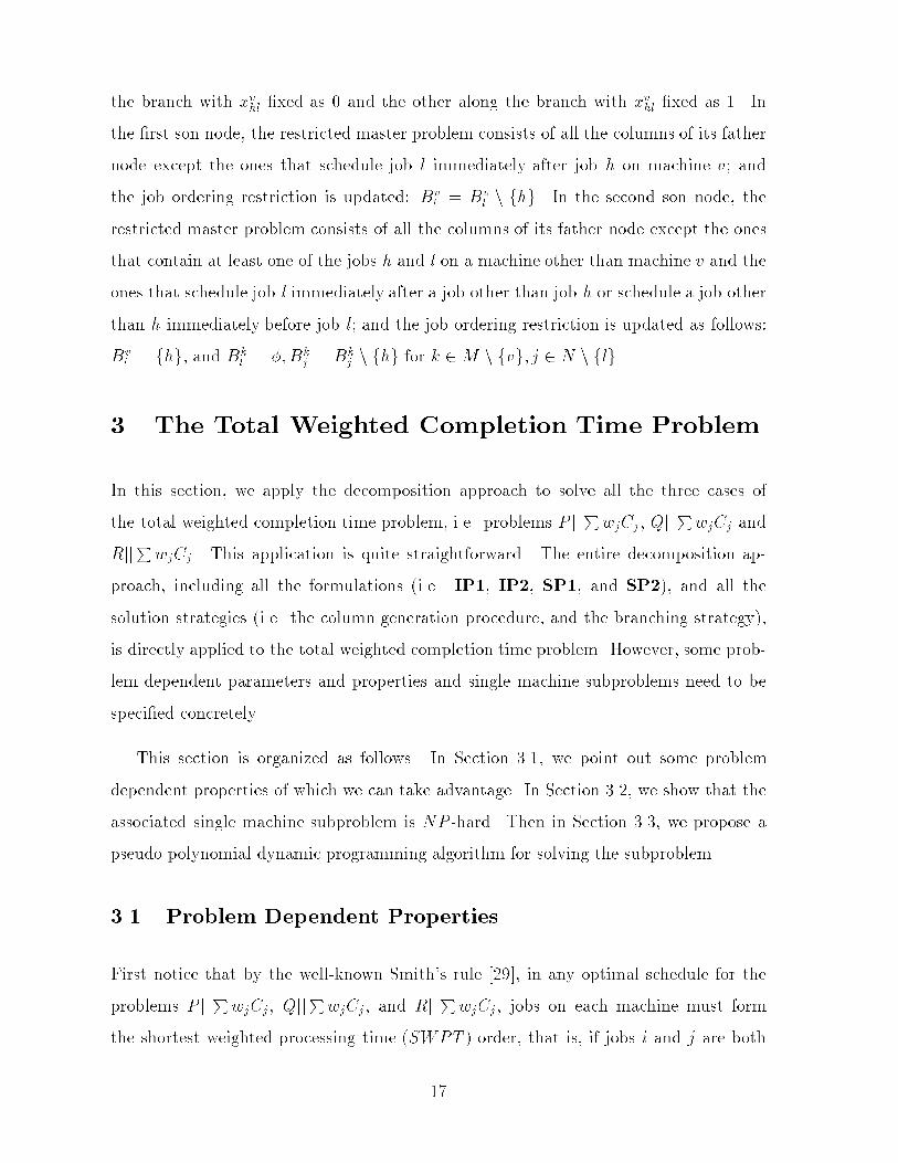
3 The Total Weighted Completion Time Problem

In this section, we apply the decomposition approach to solve all the three cases of

the total weighted completion time problem, i.e. problems P jjPwjCj , Qjj

PwjCj and

RjjPwjCj. This application is quite straightforward. The entire decomposition ap-

proach, including all the formulations (i.e. IP1, IP2, SP1, and SP2), and all the

solution strategies (i.e. the column generation procedure, and the branching strategy),

is directly applied to the total weighted completion time problem. However, some prob-

lem dependent parameters and properties and single machine subproblems need to be

speci�ed concretely.

This section is organized as follows. In Section 3.1, we point out some problem

dependent properties of which we can take advantage. In Section 3.2, we show that the

associated single machine subproblem is NP -hard. Then in Section 3.3, we propose a

pseudo-polynomial dynamic programming algorithm for solving the subproblem.

3.1 Problem Dependent Properties

First notice that by the well-known Smith's rule [29], in any optimal schedule for the

problems P jjPwjCj, Qjj

PwjCj, and Rjj

PwjCj, jobs on each machine must form

the shortest weighted processing time (SWPT ) order, that is, if jobs i and j are both

17

processed on machine k and i precedes j, then pik=wi � pjk=wj . So we need only

consider those schedules where the partial schedule on each machine forms the SWPT

order. Hence, here, a feasible partial schedule (de�ned in Section 2) is actually a partial

schedule in which jobs form the SWPT order.

Let SWPT k denote the SWPT order formed by all the jobs N on machine k.

Without loss of generality, we assume that if two jobs i and j have the same ratios:

pik=wi = pjk=wj, then the one with the smaller index precedes the other one in the

sequence SWPT k. By this assumption, the sequence SWPT k is unique for all k 2 M .

Also, it is easy to see that SWPT 1 = SWPT 2 = ::: = SWPTm for the problems

P jjPwjCj and Qjj

PwjCj. The sets A

kj , B

kj , Aj and Bj used in the formulations IP1

and IP2 are actually as follows:

Akj = fi 2 N j i succeeds j in the sequence SWPT kg

Bkj = fi 2 N j i precedes j in the sequence SWPT kg

Aj = fi 2 N j i succeeds j in the SWPT order of Ng

Bj = fi 2 N j i precedes j in the SWPT order of Ng:

Similarly, the sets k and used in the formulations SP1 and SP2 are actually as

follows:

k = f all possible partial schedules on machine k that satisfy the SWPT rule g

= f all possible partial schedules on a single machine that satisfy the SWPT rule g:

Finally, we point out that, by the de�nitions of sets k and given here and the

observation made in Section 2.2.3, a single machine subproblem on some machine is

actually to �nd a subset of jobs such that the total weighted completion time of the

jobs under the SWPT order on that machine minus the total dual variable value corre-

sponding to the jobs is minimized. We show the NP -hardness of this problem and give

a dynamic programming algorithm for it in the following subsections.

18

3.2 NP -hardness proof of the Subproblem

As mentioned in the preceding subsection, the single machine subproblem can be stated

as follows. Given a set of jobs N = f1; 2; :::; ng, a processing time pi 2 Z+, a weight

wi 2 Z+, and a dual variable value �i 2 Z, for each i 2 N , the objective is to �nd a

subset H � N such that the total weighted completion time of the jobs of H under the

SWPT sequence minus the total dual variable values corresponding to the jobs of H is

minimized. Note that in the case of QjjPwjCj or Rjj

PwjCj , the processing time pi

of job i here is replaced by pik, the processing time of i on some machine k where the

subproblem is being considered.

We show the NP -hardness of the single machine subproblem by a reduction from

the PARTITION problem, a known NP -complete problem (Garey and Johnson [15]).

An instance I of the PARTITION problem can be stated as follows:

Given n+ 1 integers, a1, a2, ..., an, and A, such that 2A =Pn

i=1 ai, does there exist

a subset S � T = f1; 2; :::; ng such thatP

j2S aj =P

j2TnS aj = A ?

Given such an instance I of the PARTITION problem, we construct a corresponding

instance II for the associated decision problem of the single machine subproblem as

follows:

� Jobs: N = T = f1; 2; :::; ng;

� Processing times: pj = aj, for all j 2 N ;

� Weights: wj = 2aj , for all j 2 N ;

� Dual variable values: �j = 2ajA+ a2j ;

� Threshold: Y = �A2.

Clearly, instance II can be constructed from instance I in polynomial time.

Theorem 1 The single machine subproblem is NP -hard in the ordinary sense.

Proof: Obviously, this problem is in the NP class. We prove its NP -hardness by

19

showing the following statement: there is a subset H � N for instance II such that the

total weighted completion time of the jobs in H under the SWPT sequence minus the

total dual variable value corresponding to the jobs inH is no greater than Y , if and only if

there is a subset S � T = f1; 2; :::; ng for instance I such thatP

j2S aj =P

j2TnS aj = A.

Then the existence of a pseudopolynomial dynamic programming algorithm (de-

scribed in the next subsection) implies that this problem is NP -hard in the ordinary

sense.

Given any subset J � N , since wj = 2pj for any j 2 N , it is easy to verify that the

total weighted completion time of the jobs of J under any sequence is:

f(J) = 2Xj2J

a2j + 2X

i<j;i;j2Jaiaj (26)

On the other hand, the total dual variable value corresponding to the jobs in J is:

g(J) =Xj2J

�j = 2AXj2J

aj +Xj2J

a2j (27)

Then the objective value of any sequence of the jobs in J is:

F (J) = f(J)� g(J) = (Xj2J

aj)2 � 2A

Xj2J

aj

= (Xj2J

aj)2 � (

Xj2J

aj +X

j2NnJaj)(

Xj2J

aj)

= �(X

j2NnJaj)(

Xj2J

aj)

� �A2 (28)

and the last equality holds if and only ifP

j2NnJ aj =P

j2J aj.

\If part". If such a subset S exists for instance I, let H = S. By the above

observation, the objective value of any sequence of the jobs in H is F (H) = �A2 = Y

sinceP

j2NnH aj =P

j2H aj. Hence the subset H is a solution to instance II.

\Only if part". If such a subset H exists for instance II, i.e. F (H) � Y = �A2. By

(28), F (H) = �A2, implying thatP

j2NnJ aj =P

j2J aj. Hence the subset S = H is a

solution to instance I. 2

20

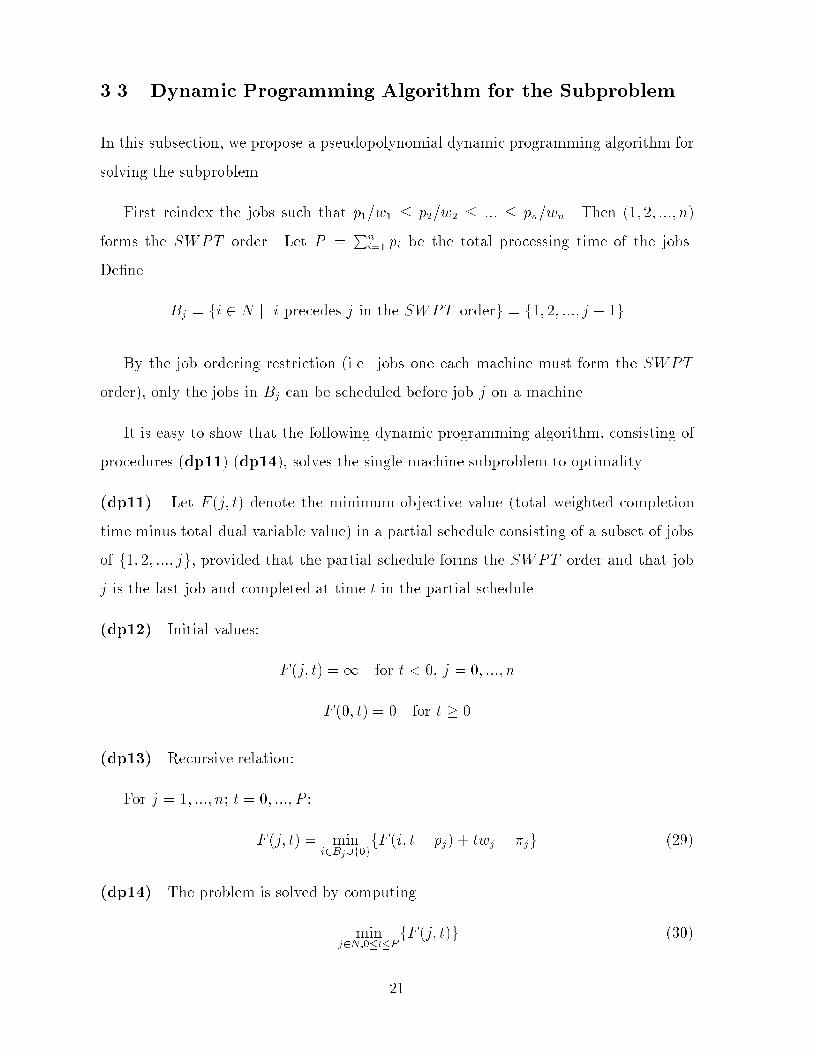
3.3 Dynamic Programming Algorithm for the Subproblem

In this subsection, we propose a pseudopolynomial dynamic programming algorithm for

solving the subproblem.

First reindex the jobs such that p1=w1 � p2=w2 � ::: � pn=wn. Then (1; 2; :::; n)

forms the SWPT order. Let P =Pn

i=1 pi be the total processing time of the jobs.

De�ne

Bj = fi 2 N j i precedes j in the SWPT orderg = f1; 2; :::; j � 1g

By the job ordering restriction (i.e. jobs one each machine must form the SWPT

order), only the jobs in Bj can be scheduled before job j on a machine.

It is easy to show that the following dynamic programming algorithm, consisting of

procedures (dp11)-(dp14), solves the single machine subproblem to optimality.

(dp11) Let F (j; t) denote the minimum objective value (total weighted completion

time minus total dual variable value) in a partial schedule consisting of a subset of jobs

of f1; 2; :::; jg, provided that the partial schedule forms the SWPT order and that job

j is the last job and completed at time t in the partial schedule.

(dp12) Initial values:

F (j; t) =1 for t < 0, j = 0; :::; n

F (0; t) = 0 for t � 0

(dp13) Recursive relation:

For j = 1; :::; n; t = 0; :::; P :

F (j; t) = mini2Bj[f0g

fF (i; t� pj) + twj � �jg (29)

(dp14) The problem is solved by computing

minj2N;0�t�P

fF (j; t)g (30)

21

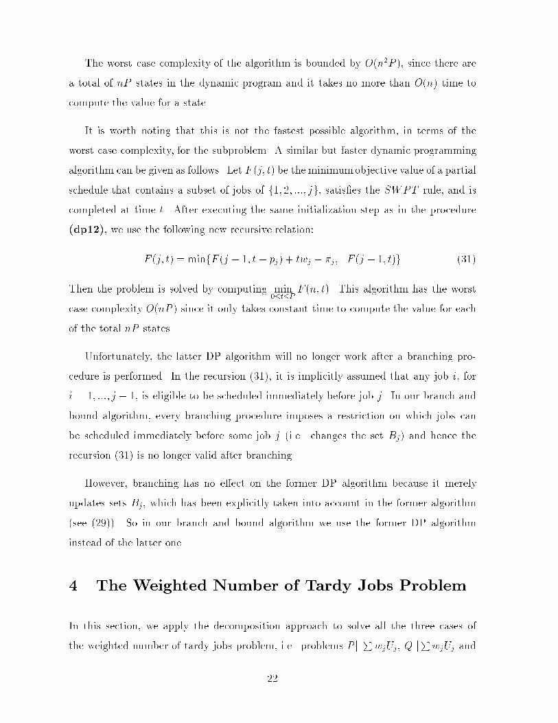
The worst case complexity of the algorithm is bounded by O(n2P ), since there are

a total of nP states in the dynamic program and it takes no more than O(n) time to

compute the value for a state.

It is worth noting that this is not the fastest possible algorithm, in terms of the

worst case complexity, for the subproblem. A similar but faster dynamic programming

algorithm can be given as follows. Let F (j; t) be the minimumobjective value of a partial

schedule that contains a subset of jobs of f1; 2; :::; jg, satis�es the SWPT rule, and is

completed at time t. After executing the same initialization step as in the procedure

(dp12), we use the following new recursive relation:

F (j; t) = minfF (j � 1; t� pj) + twj � �j; F (j � 1; t)g (31)

Then the problem is solved by computing min0�t�P

F (n; t). This algorithm has the worst

case complexity O(nP ) since it only takes constant time to compute the value for each

of the total nP states.

Unfortunately, the latter DP algorithm will no longer work after a branching pro-

cedure is performed. In the recursion (31), it is implicitly assumed that any job i, for

i = 1; :::; j � 1, is eligible to be scheduled immediately before job j. In our branch and

bound algorithm, every branching procedure imposes a restriction on which jobs can

be scheduled immediately before some job j (i.e. changes the set Bj) and hence the

recursion (31) is no longer valid after branching.

However, branching has no e�ect on the former DP algorithm because it merely

updates sets Bj, which has been explicitly taken into account in the former algorithm

(see (29)). So in our branch and bound algorithm we use the former DP algorithm

instead of the latter one.

4 The Weighted Number of Tardy Jobs Problem

In this section, we apply the decomposition approach to solve all the three cases of

the weighted number of tardy jobs problem, i.e. problems P jjPwjUj, Qjj

PwjUj and

22

RjjPwjUj.

If we apply all the formulations (i.e. IP1, IP2, SP1, and SP2) directly to the

weighted number of tardy jobs problem, then by the reduced cost formula (21), the

resulting subproblem on a machine is to �nd a partial schedule such that the total

weight of tardy jobs in the schedule minus the total dual variable value of the jobs in

the schedule is minimized. If there is no job ordering restriction, this subproblem is no

more di�cult than the well-know single machine weighted number of tardy jobs problem,

which can be solved quite e�ciently by the pseudo-polynomial dynamic programming

algorithm of Lawler and Moore [23]. However, after a branching procedure is performed,

some ordering restriction will be imposed on jobs, and no pseudopolynomial algorithm,

we believe, can solve the resulting subproblem.

Hence, to get e�cient algorithms (particularly, an algorithm for the subproblem), we

need to modify the formulations IP1, IP2, SP1, and SP2. As we will see soon, the

resulting subproblem based on the modi�ed formulations can be solved by a pseudopoly-

nomial dynamic programming algorithm, and fortunately, branching will not a�ect the

capability of the algorithm. Despite the modi�cation, the general solution strategies de-

scribed in Section 2 (i.e. the column generation procedure, and the branching strategy)

can be directly applied.

The organization of this section is as follows. In Section 4.1, we modify the formula-

tions IP1 and SP1 (IP2 and SP2 can be modi�ed similarly) and point out a result that

can be used in the branching procedure. In Section 4.2, we present a pseudo-polynomial

dynamic programming algorithm for solving the subproblem.

4.1 Modi�ed Formulations

In this subsection, we modify the formulations IP1 and SP1 (for the problemsQjjPwjUj

andRjjPwjUj). The other two formulations: IP2 and SP2 (for the problemP jj

PwjUj)

can be modi�ed similarly, and hence we do not give any detail on them.

It is clear that by the well-known result of Lawler and Moore [23], for each of the

23

problems P jjPwjUj, Qjj

PwjUj and Rjj

PwjUj , there exists an optimal schedule where

the partial schedule on each machine satis�es the following properties:

Property 1: On-time jobs form the EDD (earliest due date �rst) order, that is, the

nondecreasing order of jobs' due dates;

Property 2: Tardy jobs are in an arbitrary order;

Property 3: On-time jobs are scheduled earlier than any of its tardy jobs.

De�ne an on-time EDD partial schedule on a single machine to be a partial schedule

on that machine in which all the jobs are on-time and form the EDD order. By Prop-

erties 1, 2 and 3, we can conclude that solving the problems P jjPwjUj , Qjj

PwjUj and

RjjPwjUj is equivalent to �nding an on-time EDD partial schedule for each machine

such that the total weight of the jobs that are not covered in these partial schedules is

minimized. Those uncovered jobs can be considered tardy and scheduled arbitrarily fol-

lowing the on-time jobs. Hence, the concept of \on-time EDD partial schedule" de�ned

here is actually equivalent to that of \feasible partial schedule" de�ned in Section 2.

Based on the above observation, we modify the formulations IP1 in the following.

De�ne the following sets and 0 � 1 variables:

Aj = fi 2 N j i succeeds j in the EDD order of Ng

Bj = fi 2 N j i precedes j in the EDD order of Ng

zj = 1 if job j is scheduled tardy on some machine; 0 otherwise.

xkij = 1 if job i and j are both scheduled on-time on machine k and i is processed

immediately before job j; 0 otherwise.

xk0j = 1 if job j is scheduled �rst and on-time on machine k; 0 otherwise.

xkj;n+1 = 1 if job j is scheduled last and on-time on machine k; 0 otherwise.

Then the following integer programming formulation (IP10) solves the problems P jjPwjUj,

QjjPwjUj and Rjj

PwjUj.

24

IP10:

minXj2N

wjzj (32)

subject to

Xk2M

Xi2Bj[f0g

xkij + zj = 1; 8j 2 N (33)

Xj2N

xk0j � 1; 8k 2M (34)

Xi2Bj[f0g

xkij =X

i2Aj[fn+1gxkji; 8k 2M; j 2 N (35)

Cj =Xk2M

0@pjkxk0j + X

i2Bj

(Ci + pjk)xkij

1A ; 8j 2 N (36)

0 � Cj � dj ; 8j 2 N (37)

xkij 2 f0; 1g; 8i; j 2 N; k 2M (38)

zj 2 f0; 1g; 8j 2 N (39)

The objective function (32) seeks to minimize the weighted number of tardy jobs. Con-

straint (33) ensures that each job j is covered by at most one on-time EDD partial

schedule. If zj = 0 then job j is covered by an on-time EDD partial schedule; otherwise

it is tardy. Each tardy job j has all xkij's= 0 and Cj = 0. Constraint (34) guarantees

that each machine is utilized at most once. Constraint (36) de�nes the completion time

of each on-time job. Constraint (37) means that each on-time job must be completed

before or at its due date. Constraints (35), (36), (37) and (38) guarantee the feasibility

of the on-time EDD partial schedule on each machine.

Applying Dantzig-Wolfe decomposition to the modi�ed formulations IP10, we can

get the following set partitioning formulation SP10.

SP10:

minXj2N

wjzj (40)

subject to

Xk2M

Xs2k

akjsyks + zj = 1; 8j 2 N (41)

25

Xs2k

yks � 1; 8k 2M (42)

yks 2 f0; 1g; 8s 2 k; k 2M (43)

zj 2 f0; 1g; 8j 2 N (44)

Here k denotes the set of all possible on-time EDD partial schedules on machine k

and all other parameters and variables are de�ned similarly as in SP1.

Similarly, the column generation procedure can be applied to solve the linear relax-

ation problem LSP10 of the integer problem SP10. Let �j denote the dual variable value

corresponding to job j, for each j 2 N , in constraint (41). Then the reduced cost rks of

the column corresponding to s 2 k is given by:

rks = �Xj2N

akjs�j � �k (45)

There are m single machine subproblems. The single machine subproblem on machine

k is to �nd an on-time EDD partial schedule s 2 k on machine k such that its reduced

cost rks is minimized, that is, to �nd an on-time EDD partial schedule s 2 k on machine

k such that the total dual variable value corresponding to the jobs covered in s, i.e. the

quantityP

j2N akjs�j, is maximized.

If we consider the dual variable value corresponding to a job as the weight of that

job, then the single machine subproblem on a machine is exactly the single machine

weighted number of tardy jobs problem. It is NP -hard in the ordinary sense (Karp [19])

and can be solved by the pseudopolynomial dynamic programming algorithm of Lawler

and Moore [23]. However, we do not use Lawler and Moore's algorithm because as we

will see in the next subsection, their algorithm is hard to implement inside a branch

and bound algorithm. Instead, we propose a new dynamic programming algorithm for

solving the subproblem. This algorithm is described in the next subsection.

Finally, we note that the result in Lemma A1 still holds with respect to the modi�ed

formulations given earlier for the weighted number of tardy jobs problem. Hence, the

branching strategy suggested in Section 2 can be directly applied to all the three cases of

the weighted number of tardy jobs problem. Furthermore, for the problems QjjPwjUj

26

and RjjPwjUj , if every qij (de�ned in Section 2) resulted from solving LSP10 is integral,

then, even if the x-variable solution is fractional, it is possible to construct an integer

solution to the problem LSP10 based on the x-variable solution and q-values. This

means that as long as q-values are integral, there is no need to conduct the second stage

branching (described in Section 2). This is proved in Lemma A2 in the Appendix.

4.2 Dynamic Programming Algorithm for the Subproblem

First reindex the jobs such that d1 � d2 � ::: � dn. Then (1; 2; :::; n) forms the EDD

order. Let Bj = f1; 2; :::; j � 1g. Then only jobs in Bj can be scheduled before job j in

a feasible partial schedule on a machine. Let P =Pn

i=1 pi be the total processing time

of the jobs. Then it is easy to see that the following dynamic programming algorithm,

consisting of procedures (dp21)-(dp24), solves the subproblem to optimality.

(dp21) Let F (j; t) denote the maximum objective function value (total dual variable

value) in an on-time EDD partial schedule consisting of a subset of jobs of f1; 2; :::; jg,

provided that job j is the last job and is completed at time t in the partial schedule.

(dp22) Initial values:

F (j; t) = �1 for t < 0, j = 0; :::; n

F (0; t) = 0 for t � 0

(dp23) Recursive relation:

For j = 1; :::; n; t = 0; :::; P :

F (j; t) = maxi2Bj[f0g

fF (i; j; t)g; (46)

where

F (i; j; t) =

(F (i; t� pj) + �j; if t � dj

�1; otherwise(47)

(dp24) The problem is solved by computing

maxj2N;0�t�P

fF (j; t)g (48)

27

The worst case complexity of the algorithm is bounded by O(n2P ), since there are

a total of nP states in the dynamic program and it takes no more than O(n) time to

compute the value for a state.

Lawler and Moore's algorithm is faster than the above algorithm in terms of the

worst case complexity. Their algorithm consists of similar procedures as in the above

algorithm. The procedure (dp22) is not changed. In (dp21), rede�ne F (j; t) to be

the maximum objective function value (total dual variable value) of an on-time EDD

partial schedule that contains a subset of jobs of f1; 2; :::; jg and is completed at time t.

In (dp23), a new recursive relation is used:

F (j; t) = maxfF (j � 1; t); F (j; t)g; (49)

where

F (j; t) =

(F (j � 1; t� pj) + �j; if t � dj

�1; otherwise(50)

Then the problem is solved by computing max0�t�P F (n; t). This algorithm has the

worst case time complexity O(nP ) since it only takes constant time to compute the

value for each of the total nP states.

Unfortunately, Lawler and Moore's algorithm will no longer work after a branching

procedure is performed. In the recursion (49), it is implicitly assumed that any job i, for

i = 1; :::; j � 1, is eligible to be scheduled immediately before job j. In our branch and

bound algorithm, every branching procedure imposes a restriction on which jobs can be

scheduled immediately before some job j (i.e. changes set Bj), and hence the recursion

(49) is no longer valid after branching. This is the reason why we do not use Lawler and

Moore's algorithm for solving the subproblem.

However, branching has no e�ect on the DP algorithm we proposed here because it

merely updates sets Bj, which has been explicitly taken into account in the procedure

(46) in our algorithm.

28

5 Computational Experiments

In this section, we describe our computational experiments for both the total weighted

completion time problem and the total weighted number of tardy jobs problem. Our

algorithms are all coded in C and tested on a Silicon Graphics Iris Workstation with

MIPS R4400 Processor. Linear programs inside the branch and bound algorithms are

solved by CPLEX, a commercial LP solver.

5.1 Con�guration of Test Problems

For the total weighted completion time problem, the test problems are generated as

follows:

� Number of machines (m). We use six di�erent numbers: 2, 4, 8, 12, 16, 20.

� Number of jobs (n). We use six di�erent numbers: 20, 30, 40, 60, 80, 100.

� Weights (wj). The weight for each job is an integer number uniformly drawn

from [1; 100].

� Processing times (pij). For the problem P jjPwjCj , the processing time pj of each

job j is an integer number uniformly drawn from [1; 10]. For the problemQjjPwjCj , the

processing time of each job j on machine i, pij = pisj, where pi and sj are both integers

from the uniform distribution [1; 10]. For the problem RjjPwjCj , pij is an integer from

the uniform distribution [1; 30].

Note that the processing times and weights in the test problems we use here for

the problem P jjPwjCj have the same distributions as the ones used in Belouadah and

Potts [4].

For the total weighted number of tardy jobs problem, the test problems are generated

as follows:

� Number of machines (m). We use �ve di�erent numbers: 2, 4, 6, 8, 10.

29

� Number of jobs (n). We use nine di�erent numbers: 20, 30, 40, 50, 60, 70, 80,

90, 100.

� Weights (wj). The weight for each job is an integer number uniformly drawn

from [1; 100].

� Processing times (pij). For the problem P jjPwjUj, processing times pi are

integers uniformly drawn from [1; 100]. For the problem QjjPwjUj, processing times

pij = pisj are generated by letting pi and sj be integers uniformly distributed in [1; 40]

and [1; 5]. For the problem RjjPwjUj , processing times pij are integers uniformly

distributed in [1; 100].

� Due dates (dj). We follow the model used in Ho and Chang [17, 18] to generate

due dates. The due date of job i is set to be maxf�i; �qg, where �i = minj2Mfpijg,

and �q is an integer uniformly distributed in [1; 100r=q] with r = n=m and q being

a controllable parameter. The q value indicates the congestion level of the scheduling

system. The larger the q, the more congested the system will be, and the more tardy

jobs will result. We consider �ve possible values for q: 1, 2, 3, 4, and 5.

5.2 Computational Results

Tables 1, 2, 3, 4, 5, and 6 list the computational results for the problems P jjPwjCj,

QjjPwjCj, Rjj

PwjCj, P jj

PwjUj, Qjj

PwjUj, and Rjj

PwjUj , respectively. In these

tables, the �rst two columns \m" and \n" represent, respectively, the number of ma-

chines and the number of jobs of a test problem. For each selected pair of values m

and n, 20 problems are randomly generated based on the distributions of the associated

parameters (for the problems P jjPwjUj, Qjj

PwjUj , and Rjj

PwjUj , exactly 4 ran-

domly generated problems have the same q value). Each of the other entries in these

tables represents an averaged performance value based on 20 problems with the same

m and n. The column \LP-IP gap" represents the average gap in percentage between

the linear relaxation solution value of the root b&b node and the integer solution value.

This percentage re ects the tightness of the lower bound obtained by solving the linear

30

relaxation problem LSP1 or LSP2 (with respect to the original integer problem SP1

or SP2). The column \problems solved at root node" indicates the number of problems

solved at the root b&b node, i.e. without any branching, out of 20 problems. The

column \b&b nodes explored" represents the average number of b&b nodes explored for

solving the problem. Note that at least one b&b node (the root node) must be explored

for solving any problem. The other two columns \columns generated" and \cpu time"

represent, respectively, the average number of columns generated for solving the problem

and the average cpu time (in seconds) consumed.

We note that among the 20 problems tested for each problem size, the worst-case of

each above mentioned performance measure is always very close to the average, so we

do not give the worst-case values of these performance measures.

From these tables, we can make the following observations:

� We can conclude that the lower bound given by the solution value of the linear

relaxation problem LSP1 (or LSP2) is extremely close to the solution value of the

integer problem SP1 (or SP2). In fact, in the case of the total weighted completion

time problem, 52% of the 1380 problems we have tested here are solved at root node

without any branching, and for each set of 20 test problems with the same size, the

average gap between the lower bound and the integer solution value is less than 0:1%.

In the case of the weighted number of tardy jobs problem, this average gap between is

less than 0:8%. Due to this excellent lower bounding, an average of only nine b&b nodes

are explored for solving an instance of the total weighted completion time problem in our

experiments. Compared to the experiments by Belouadah and Potts [4] where at least

thousands of b&b nodes have to be explored for solving a problem with a similar size,

we can evidently conclude that our lower bound is much tighter than that in Belouadah

and Potts [4] using Lagrangian relaxation. We note that, however, to solve a b&b node,

our algorithm may take longer time than the algorithm by Belouadah and Potts.

� For the problem P jjPwjCj, our algorithm is capable of solving the problems

twice the size of the ones solved in the literature ([28], [4]) in a reasonable time. For the

31

other problems (on which no computational results are reported in the literature), our

algorithm is capable of solving instances with a similar size in a similar time as well.

� Our algorithm works extremely well when the ratio of the number of jobs to the

number of machines (n=m) is relatively small (say, less than eight). When this ratio is big

(say, more than ten), the column generation procedure su�ers from degeneracy (i.e. the

dual information provided by solving a restricted master problem is not accurate enough

and hence many columns generated are not very useful) and the algorithm becomes

relatively slow even for problems with a small number of machines. For example, the

average cpu time for a problem with m = 8 and n = 60 is much lower than that for a

problem with m = 4 and n = 60.

6 Conclusion

We have developed a decomposition approach that can be applied to solve to optimality

virtually every classical parallel machine scheduling problem with an additive criterion

for which single machine subproblems admit an e�cient solution. The applications of

this decomposition approach to the total weighted completion time problem and the

weighted number of tardy jobs problem have shown that the approach is promising and

capable of solving large problems.

However, in order to apply this decomposition approach e�ciently to a particular

problem, it is important to give proper IP and SP formulations to the problem. As we

have seen, for some problems, such as the total weighted completion time problem, the

general IP and SP formulations described in Section 2 can be directly followed, while

for some other problems, such as the weighted number of tardy jobs problem, it may

be necessary to (slightly) modify these general formulations so that the resulting single

machine subproblems can be more tractable.

Naturally, an interesting research topic is to apply the decomposition approach to

other parallel machine scheduling problems with an additive criterion, such as the total

(weighted) tardiness problem, the total earliness-tardiness penalty problem, etc. Actu-

32

ally, we have just successfully applied this approach to the latter problem with a common

due date (Chen and Powell [8]).

Another possible research topic is to design fast heuristics for more complex parallel

machine scheduling problems, e.g. the problems considered here with additional con-

straints, based on the idea of the decomposition approach. One possible way on this line

of research is to use a heuristic, instead of an exact algorithm, to solve single machine

subproblems.

Appendix

Lemma A1 Given a y-variable solution (yks ; s 2 k; k 2 M) to LSP1 or (ys; s 2 )

to LSP2, if the corresponding x-variable solution given by (23) or (24) is integral, then

the y-variable solution must be integral.

Proof: We prove the result by contradiction for the case of LSP1. For the case of LSP2,

it can be similarly proved. Let

Sk =ns 2 k j yks > 0

o

Since columns generated in the column generation procedure are always distinct, all the

schedules in Sk must be distinct. Suppose that there exists some machine k and some

schedule s 2 Sk such that yks is fractional, i.e. 0 < yks < 1. Without loss of generality,

we assume that jobs i and j are two adjacent jobs in s and i precedes j, where i can be

0, meaning that job j is the �rst one in s. Thus, by (23), xkij > 0, which indicates that

xkij = 1 by the fact that the x-variable solution is integral. Since 0 < yks < 1, there must

exist another schedule u 2 Sk with yku > 0 in which j follows i immediately. Since the

two schedules s and u are distinct, there must exist three jobs a; b; c such that b follows

a immediately in s while b follows c immediately in u. This implies that xkab > 0 and

xkcb > 0, which further implies that

xkab = 1; and xkcb = 1

33

HenceP

i2Bkb[f0g x

kib � 2. On the other hand, the equations (23) and (14) implies thatP

i2Bkb[f0gx

kib � 1. This leads to a contradiction. Therefore, the y-variable solution must

be integral. 2

Lemma A2 Given a y-variable solution (yks ; s 2 k; k 2 M) to the problem LSP10,

if the corresponding q-values given by (23) and (25) are all integral, then an integer

solution to the problem LSP10 can be constructed from the known values of y and x.

Proof: First we need to give a de�nition that will be used later. Two single machine

partial schedules are said to be identical if they contain the same subset of jobs and form

the same sequence (but they may be on di�erent machines).

De�ne

� = fs 2 k, for some k 2M j yks > 0g;

E = fj 2 N j j is covered by some schedule in �g;

H = fj 2 N j q0j = 1g = fl1; l2; :::; ljHjg;

�h = fs 2 � j es0h = 1, i.e. job h is scheduled �rst in schedule sg, where esij is de�ned

to be 1 if job j is scheduled immediately after job i in s.

Let F (y) be the objective function value of LSP10 corresponding to the solution (yks ; s 2

k; k 2M). By (23), (25) and (41), the following relations can be easily proved:

Xi2Bj[f0g

qij =Xk2M

Xs2k

akjsyks =

(1; if j 2 E0; otherwise

(51)

and

F (y) =X

j2NnEwj (52)

Hence, each qij 2 f0; 1g.

Similarly, by (23), (25) and (41), it is not di�cult to show the following results:

(1) jHj � m

34

(2) All the partial schedules in �h, for each h 2 H, are identical, and hence �h

contains only one partial schedule. Denote this schedule as �h.

(3) These jHj partial schedules �1, ..., �jHj are disjoint and cover all the jobs in E.

Now we need to show that these jHj partial schedules �1, ..., �jHj form an integer

solution to the problem LSP10. The key issue we need to resolve here is to �nd what

machine to process �h, for each h 2 H. De�ne, for each h 2 H,

Mh = fk 2M j�h 2 k; yk�h > 0g.

The machines in Mh are in fact the candidates for processing schedule �h. Given any

subset L � H, let M(L) =[l2L

Ml. It is easy to see that

Xj2L

q0j =Xj2L

Xk2M

Xs2k

es0jyks

=Xj2L

Xk2Mj

yk�j

�Xs2

Xk2M(L)

yks

� jM(L)j (53)

On the other hand,P

j2L q0j = jLj. Thus jLj � jM(L)j. De�ne a bipartite graph

G(X;Y ) with vertex set X = HSM and edge set Y = f(h; k)jh 2 H; k 2 Mhg. Then

by the well-known Hall's Theorem (see, e.g. Bondy and Murty [5]), the bipartite graph G

contains a matching that saturates every vertex in H. This means that for any h 2 H,

we can �nd a proper machine mh 2 M to process schedule �h. More precisely, the

problem LSP10 is solved by the integer solution (yks ; s 2 k; k 2 M) with ymh�h

= 1 for

any h 2 H and yks = 0 for any other pair (s; k). Since all the jobs in E are covered by

the schedules in[h2H

�h, thus the objective function value corresponding to this integer

solution isX

j2NnEwj = F (y). This means that this integer solution is optimal too. 2

35

Table 1: Computational results for P jjPwjCj

problem LP-IP problems solved b&b nodes columns cpu timem n gap at root node explored generated (in seconds)

2 20 0.0% 20 1 471 2.142 30 0.0% 14 1.4 1735 27.322 40 0.0% 12 1.3 4396 183.91

4 20 0.0% 20 1 274 0.474 30 < 0:001% 13 1.8 794 4.964 40 < 0:001% 7 3.0 1566 23.344 60 < 0:001% 3 14.2 8712 523.154 80 < 0:001% 3 16.3 1427 1723.49

8 20 0.0% 20 1 153 0.138 40 0.0% 17 1.2 896 3.098 60 < 0:001% 6 10.4 1891 54.728 80 < 0:001% 0 25.3 6958 447.298 100 < 0:001% 0 48.0 13518 1524.50

12 40 0.0% 20 1 552 0.7812 60 0.0% 8 7.4 1761 18.7112 80 0.0% 0 20.5 3544 119.1812 100 0.0% 0 32.3 7589 467.82

16 40 0.0% 20 1 473 0.4116 60 0.0% 13 3.0 1297 5.1316 80 < 0:001% 3 14.4 1917 40.7816 100 < 0:001% 0 55.2 6006 276.61

20 60 0.0% 20 1 930 1.6320 80 0.0% 4 9.0 2003 20.1220 100 0.0% 0 20.4 4903 96.45

36

Table 2: Computational results for QjjPwjCj

problem LP-IP problems solved b&b nodes columns cpu timem n gap at root node explored generated (in seconds)

2 20 0.0% 20 1 723 3.172 30 0.0% 20 1 2159 45.352 40 0.0% 20 1 2487 202.74

4 20 0.019% 18 1.3 625 1.474 30 0.012% 13 2.6 1540 10.234 40 0.025% 5 3.3 3521 87.464 60 0.014% 0 10.0 8435 1184.33

8 20 0.0% 20 1 756 0.748 40 < 0:001% 15 1.1 1857 17.838 60 0.072% 0 3.2 7551 663.878 80 0.0152% 0 25.6 11815 2898.49

12 40 0.039% 10 3.3 3317 17.5312 60 < 0:001% 3 5.1 8497 176.3412 80 0.013% 0 13.8 13021 746.1812 100 0.012% 0 22.1 21908 2109.39

16 40 0.0% 20 1 3445 8.6516 60 0.054% 0 23.5 8032 184.1316 80 0.004% 0 27.0 6940 512.8716 100 0.006% 0 30.7 9362 1267.56

20 60 0.033% 2 13.5 7311 35.4520 80 0.029% 0 38.0 12970 551.7820 100 0.073% 0 45.8 16375 1320.71

37

Table 3: Computational results for RjjPwjCj

problem LP-IP problems solved b&b nodes columns cpu timem n gap at root node explored generated (in seconds)

2 20 0.0% 20 1 664 2.082 30 0.0% 20 1 2021 47.822 40 0.0% 20 1 4629 436.39

4 20 0.0% 20 1 489 0.944 30 0.0% 18 1.2 1403 8.964 40 0.0% 20 1 2539 51.154 60 0.0% 10 3.4 7271 623.35

8 20 0.0% 20 1 529 0.948 40 0.0% 20 1 1728 10.128 60 0.002% 17 1.1 3720 87.978 80 < 0:001% 15 1.2 7001 487.418 100 < 0:001% 15 1.2 12906 2050.93

12 40 0.0% 20 1 1579 6.5612 60 0.0% 20 1 3340 48.0212 80 < 0:001% 10 7.1 5724 203.3412 100 0.016% 3 6.4 9362 1043.57

16 40 0.0% 20 1 1394 5.4016 60 < 0:001% 17 2.4 3174 44.8516 80 0.002% 6 2.0 5394 206.4216 100 0.0015% 5 3.4 7981 523.59

20 60 0.0% 20 1 2731 27.2320 80 0.032% 12 4.5 4858 140.9220 100 < 0:001% 9 5.6 6930 362.80

38

Table 4: Computational results for P jjPwjUj

problem LP-IP problems solved b&b nodes columns cpu timem n gap at root node explored generated (in seconds)

2 20 0.0% 12 1.6 89 0.062 30 0.03% 10 2.4 537 3.772 40 0.12% 5 3.4 1320 28.122 50 0.22% 2 8.3 2689 176.93

4 20 0.0% 20 1.0 99 0.064 30 0.49% 9 2.1 505 0.924 40 0.56% 3 8.7 993 7.544 50 0.56% 0 25.8 3202 114.404 60 0.26% 0 81.2 10036 682.35

6 30 0.07% 11 1.4 176 0.216 40 0.04% 4 5.0 391 1.706 50 0.23% 0 19.7 1747 18.066 60 0.31% 0 43.5 4349 93.626 70 0.20% 0 61.0 6231 273.786 80 0.16% 0 117.5 9407 835.29

8 40 0.15% 7 3.3 379 1.618 50 0.10% 2 12.5 1556 8.348 60 0.34% 0 43.0 2387 55.228 70 0.27% 0 65.9 4021 97.748 80 0.33% 0 94.3 7139 305.40

10 40 0.0% 20 1.0 209 0.1110 50 0.0% 8 4.6 774 1.9510 60 0.25% 3 15.5 1119 12.5010 70 0.25% 0 35.6 2031 33.6310 80 0.23% 0 69.5 4057 95.1210 90 0.16% 0 81.7 7671 286.9510 100 0.08% 0 100.4 11456 1206.27

39

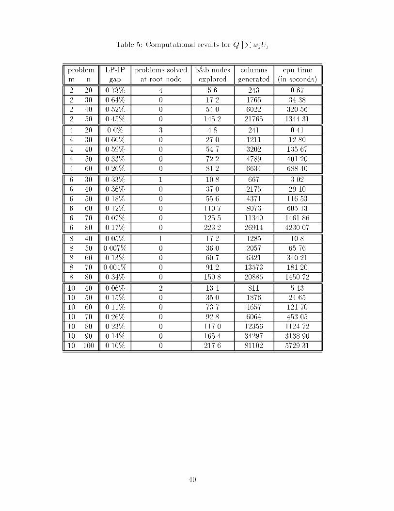
Table 5: Computational results for QjjPwjUj

problem LP-IP problems solved b&b nodes columns cpu timem n gap at root node explored generated (in seconds)

2 20 0.73% 4 5.6 243 0.672 30 0.64% 0 17.2 1765 34.382 40 0.52% 0 54.0 6022 320.562 50 0.45% 0 145.2 21765 1344.31

4 20 0.0% 3 4.8 241 0.414 30 0.60% 0 27.0 1211 12.804 40 0.59% 0 54.7 3202 135.674 50 0.33% 0 72.2 4789 401.204 60 0.26% 0 81.2 6634 688.40

6 30 0.33% 1 10.8 667 3.026 40 0.36% 0 37.0 2175 29.406 50 0.18% 0 55.6 4371 116.536 60 0.12% 0 110.7 8073 605.136 70 0.07% 0 125.5 11340 1461.866 80 0.17% 0 223.2 26914 4230.07

8 40 0.05% 1 17.2 1285 10.88 50 0.007% 0 36.0 2057 65.768 60 0.13% 0 60.7 6321 340.218 70 0.004% 0 91.2 13573 181.208 80 0.34% 0 150.8 20886 1450.72

10 40 0.06% 2 13.4 811 5.4310 50 0.15% 0 35.0 1876 24.6510 60 0.11% 0 73.7 4657 121.7010 70 0.26% 0 92.8 6064 453.0510 80 0.23% 0 117.0 12356 1124.7210 90 0.14% 0 165.4 34297 3138.9010 100 0.10% 0 217.6 81102 5729.31

40

Table 6: Computational results for RjjPwjUj

problem LP-IP problems solved b&b nodes columns cpu timem n gap at root node explored generated (in seconds)

2 20 0.09% 7 2.4 271 0.472 30 0.11% 7 2.6 854 5.802 40 0.09% 6 3.4 1509 38.052 50 0.12% 1 10.6 4763 257.25

4 20 0.0% 17 1.2 135 0.134 30 0.22% 5 5.4 653 1.684 40 0.02% 2 12.2 1460 11.604 50 0.15% 0 77.8 8756 273.174 60 0.10% 0 132.6 17919 1388.40

6 30 0.0% 9 2.6 203 0.386 40 0.01% 2 6.8 444 1.726 50 0.01% 0 27.6 2185 30.346 60 0.004% 0 63.8 6241 169.206 70 0.08% 0 99.7 9073 435.846 80 0.09% 0 156.4 14658 1022.43

8 40 0.005% 2 10.8 695 2.818 50 < 0:001% 0 36.0 2057 25.428 60 < 0:001% 0 52.4 4743 118.378 70 0.003% 0 83.2 5439 181.208 80 0.001% 0 103.9 11368 849.61

10 40 0.0% 1 9.2 485 2.2510 50 < 0:001% 0 18.8 963 7.2310 60 < 0:001% 0 26.6 1738 26.0810 70 0.006% 0 41.8 3864 123.4510 80 0.02% 0 103.4 8107 466.8110 90 0.02% 0 125.1 14297 1221.0410 100 0.05% 0 178.2 42603 3287.52

41

Acknowledgement

This research was supported in part by grant AFOSR-F49620-93-1-0098 from the Air

Force O�ce of Scienti�c Research. The authors would like to thank the two anonymous

referees for their helpful comments and suggestions on the earlier version of this paper.

References

[1] K.R. Baker. Introduction to Sequencing and Scheduling. Wiley, New York, 1974.

[2] J.W. Barnes and J.J. Brennan. An improved algorithm for scheduling jobs onidentical machines. AIIE Transactions, 9:25{31, 1977.

[3] C. Barnhart, E. Johnson, G.L. Nemhauser, M.W.P. Savelsbergh, and P. H. Vance.Branch-and-price: Column generation for solving huge integer programs. In J.R.Birge and K.G. Murty, editors, Mathematical Programming: State of the Art 1994,pages 186{207. The University of Michigan, 1994.

[4] H. Belouadah and C.N. Potts. Scheduling identical parallel machines to minimizetotal weighted completion time. Discrete Applied Mathematics, 48:201{218, 1995.

[5] J.A. Bondy and U.S.R. Murty. Graph Theory with Applications. Elsevier SciencePublishing Co., Inc., North Holland, 1976.

[6] D. Cattrysse, M. Salomon, R. Kuik, and L.N. Van Wassenhove. A dual ascent andcolumn generation heuristic for the discrete lotsizing and scheduling problem withsetup times. Management Science, 39(4):477{486, 1993.

[7] L.M.A. Chan, P. Kaminsky, A. Muriel, and D. Simchi-Levi. Machine scheduling,linear programming and list scheduling heuristic. Technical report, NorthwesternUniversity, Chicago, 1995.

[8] Z.-L. Chen and W.B. Powell. A decomposition approach for a parallel machine just-in-time scheduling problem. Technical report, Statistics and Operation Research,Princeton University, 1996.

[9] T.C.E. Cheng and C.C.S. Sin. A state-of-the-art review of parallel-machine schedul-ing research. European Journal of Operational Research, 47:271{292, 1990.

[10] G.B. Dantzig and P. Wolfe. Decomposition principle for linear programs. OperationsResearch, 8:101{111, 1960.

[11] P. De, J.B. Ghosh, and C.E. Wells. Due-date assignment and early/tardy schedulingon identical parallel machines. Naval Research Logistics, 41:17{32, 1994.

[12] M. Desrochers, J. Desrosiers, and M. Solomon. A new optimization algorithm forthe vehicle routing problem with time windows. Operations Research, 40:342{354,1992.

[13] W.L. Eastman, S. Even, and I.M. Isaacs. Bounds for the optimal scheduling of njobs on m processors. Management Science, 11:268{279, 1974.

42

[14] S.E. Elmaghraby and S.H. Park. Scheduling jobs on a number of identical machines.AIIE Transactions, 6:1{12, 1974.

[15] M.R. Garey and D.S. Johnson. Computers and Intractability: A Guide to the Theoryof NP-Completeness. Freeman, San Francisco, CA, 1979.

[16] P.C. Gilmore and R.E. Gomory. A linear programming approach to the cutting-stock problem. Operations Research, 9:849{859, 1961.

[17] J.C. Ho and Y.-L. Chang. Heuristics for minimizing mean tardiness for m parallelmachines. Naval Research Logistics, 38:367{381, 1991.

[18] J.C. Ho and Y.-L. Chang. Minimizing the number of tardy jobs for m parallelmachines. European Journal of Operational Research, 84:343{355, 1995.

[19] R.M. Karp. Reducibility among combinatorial problems. In R.E. Miller and J.W.Thatcher, editors, Complexity of Computations, New York, 1972. Plenum Press.

[20] L.S. Lasdon. Optimization Theory for Large Systems. MacMillan, New York, 1970.

[21] S. Lavoie, M. Minoux, and E. Odier. A new approach for crew pairing problemsby column generation with an application to air transport. European Journal ofOperational Research, 35:45{58, 1988.

[22] E.L. Lawler, J.K. Lenstra, A.H.G. Rinnooy Kan, and D.B. Shmoys. Sequencingand scheduling: Algorithms and complexity. In S.C. Graves, A.H.G. Rinnooy Kan,and P.H. Zipkin, editors, Logistics of Production and Inventory, Amsterdam, 1993.North Holland.

[23] E.L. Lawler and J.M. Moore. A functional equation and its applications to resourceallocation and sequencing problems. Management Science, 16:77{84, 1969.

[24] A. Mehrotra and M.A. Trick. A column generation approach to graph coloring.Technical report, Graduate School of Industrial Administration, Carnegie MellonUniversity, Pittsburgh, PA, 1993.

[25] G. Nemhauser and L. Wolsey. Integer and Combinatorial Optimization. John Wiley& Sons, Inc., Chichester, 1988.

[26] M. Pinedo. Scheduling: Theory, Algorithm, and System. Prentice Hall, EnglewoodCli�s, NJ, 1995.

[27] M.H. Rothkopf. Scheduling independent tasks on parallel processors. ManagementScience, 12:437{447, 1966.

[28] S.C. Sarin, S. Ahn, and A.B. Bishop. An improved scheme for the branch andbound procedure of scheduling n jobs on m parallel machines to minimize totalweighted owtime. International Journal of Production Research, 26(7):1183{1191,1988.

[29] W.E. Smith. Various optimizer for single-stage production. Naval Research LogisticsQuarterly, 3:59{66, 1956.

[30] J.M. van den Akker, J.A. Hoogeveen, and S.L. van de Velde. Parallel machinescheduling by column generation. Technical report, Center for Operations Researchand Econometrics, Universite Catholique de Louvain, Belgium, 1995.

43

[31] P.H. Vance. Crew scheduling, cutting stock, and column generation: Solving hugeinteger programs. Technical report, PhD dissertation, School of Industrial andSystems Engineering, Georgia Institute of Technology, Atlanta, Georgia, 1993.

[32] P.H. Vance, C. Barnhart, E.L. Johnson, and G.L. Nemhauser. Solving binary cut-ting stock problems by column generation and branch-and-bound. ComputationalOptimization and Applications, 3:111{130, 1994.

[33] S. Webster. New bounds for the identical parallel processor weighted ow timeproblem. Management Science, 38(1):124{136, 1992.

[34] S. Webster. A priority rule for minimizing weighted ow time in a class of parallemachine scheduling problems. European Journal of Operational Research, 70:327{334, 1993.

[35] S. Webster. Weighted ow time bounds for scheduling identical processors. EuropeanJournal of Operational Research, 80:103{111, 1995.

44