1 Evaluation of Optimum SIMO Combining for Estimated and...

1

Evaluation of Optimum SIMO Combining for

Estimated and Correlated Rician Fading

Constantin Siriteanu, Yoshikazu Miyanaga, and Steven D. Blostein

Abstract

This analysis extends to Rician fading our earlier studies for Rayleigh fading of maximal-ratio

eigencombining (MREC) — also known as eigenbeamforming — vs. maximal-ratio combining (MRC)

and statistical beamforming (BF), for single-input multiple-output (SIMO) wireless systems. MREC is

a superset of BF and MRC. Given instantaneous channel state information (ICSI), which is the channel

gain vector estimate, and statistical CSI, which is determined by the Rician K-factor and the azimuth

spread (AS), we analyze the optimum combining approach (instead of the commonly-studied suboptimal

combining approach) based on the distribution of the effective signal-to-noise ratio. An expression is

derived for the average error probability (AEP) of MREC in correlated Rician fading when antenna

K-factors may be unequal. This AEP also applies for MRC and BF with estimated ICSI. Furthermore,

a new bias–variance tradeoff criterion (BVTC) is proposed for MREC adaptation not only to AS (as

with existing criteria), but also to K and ICSI accuracy. First, we demonstrate that BVTC-based adaptive

MREC can achieve near-MRC AEP performance and lower numerical complexity. Furthermore, we find

that the results of the realistic MREC performance and complexity evaluation approach, i.e., averaging

over measured K distribution, are substantially different than the results of the conventional evaluation

approach, i.e., setting K to typical value (distribution average or zero).

Index Terms

Azimuth spread, channel estimation, correlated fading, eigencombining, Rician K-factor.

This work was presented, in part, at the International Conference on Green Circuits and Systems, Shanghai, China, 2010.

Constantin (Costi) Siriteanu is GCOE Assistant Professor, Graduate School of Information Science and Technology, Hokkaido

University, Sapporo, Japan. E-mail: [email protected]

Yoshikazu Miyanaga is Professor, Graduate School of Information Science and Technology Hokkaido University, Sapporo,

Japan. E-mail: [email protected]

Steven D. Blostein is Professor, Department of Electrical and Computer Engineering, Queen’s University, Kingston, Canada.

E-mail: [email protected]

September 1, 2010 DRAFT

2

I. INTRODUCTION

A. Background on Eigencombining and Fading Models

The multi-antenna transceiver concept has evolved over the last few decades to become

mainstream in wireless area networks and cellular systems. This evolution has been punctuated

by groundbreaking studies into its benefits and challenges [1] [2] [3] [4] [5].

Originally, researchers sought to achieve: 1) diversity gain, with receive diversity arrays,

assuming decorrelated signals, e.g., for cellular links characterized by multipath [1]; diversity

combining requires instantaneous channel state information (ICSI); 2) array gain, with receive-

side beamforming phased-arrays, assuming near-coherent received signals, e.g., for radar links

characterized by line-of-sight (LOS) [2] [3]; beamforming requires statistical CSI (SCSI) .

However, signals are typically received with power azimuth spread (PAS) of scenario-dependent

width, i.e., azimuth spread (AS) [6] [7]. Therefore, more recently, classical diversity and beam-

forming concepts have been unified, by exploiting both ICSI and SCSI, under the framework of

statistical eigenbeamforming [8] [9] [10], which we refer to as eigencombining for single-input

multiple-output (SIMO) systems [11] [12] [13] [14] [15, Chapter 1] [16].

Statistical eigenbeamforming promises better average error probability (AEP) performance and

lower numerical complexity by adapting processing to propagation conditions through SCSI, for

SIMO [13] [14] [16] as well as for multiple-input single-output (MISO) and multiple-input

multiple-output (MIMO) systems [17] [18].

Previous eigencombining evaluations have typically adopted the tractable Rayleigh fading

channel model [13] [14] [16] [17] [18]. However, measurements have shown that many scenarios

experience Rician fading [7] [19] [20] [21], which is characterized by the K-factor, i.e., the

deterministic-vs.-random channel-component power ratio. Furthermore, measured K-factor and

AS have lognormal distributions with scenario-dependent parameters and correlation [6] [7]

[19] [20]. Therefore, herein, we evaluate the performance–complexity trade-offs achievable with

eigencombining for a Rician channel fading model supported by recent measurements [7].

B. Terminology, Methods, and Models

Terminology is now introduced for the combining methods, ICSI estimation approaches,

channel fading, AS, and K models, and eigencombining adaptation techniques considered herein.


3

• Signal–channel combining (hereafter, combining) principles, given perfect ICSI and SCSI:

– Maximal-ratio combining (MRC): (diversity) combines the received signal vector and

channel gain vector to maximize the symbol-detection signal-to-noise ratio (SNR) [1].

On the transmit side, this is known as maximal-ratio transmission for MISO [22,

Section 5.4.2] and one-dimensional eigenbeamforming for MIMO [18].

– Statistical beamforming (BF): combines the received signal vector and dominant channel-

covariance-matrix eigenvector [23] [24, Section 9.2.2]. On the transmit side, this is

known as statistical one-dimensional beamforming for MISO and MIMO [17] [18].

– Maximal-ratio eigencombining (MREC): projects the received signal vector onto dom-

inant eigenvectors (i.e., Karhunen-Loeve Transform — KLT), then applies MRC [8]

[9] [10] [11] [13] [15, Chapter 1] [14] [16]. MREC is a superset of MRC and BF [12]

[13] [25]. On the transmit side, this is known as two-dimensional eigenbeamforming

and statistical linear precoding for MISO and MIMO [17] [18].

• ICSI estimation methods based on pilot-symbol-aided modulation (PSAM) and:

– Minimum mean-square error (optimum) interpolation, i.e., MMSE PSAM

– Sinc-function (suboptimum) interpolation, i.e., SINC PSAM [11] [26] [27] [28] [29].

• Combining approaches, given estimated ICSI and perfect SCSI:

– Optimum (i.e., exact) combining [30] [31] [32] [13] [33]

– Suboptimum (i.e., approximate) combining [34] [28] [35] [29].

• Channel fading models:

– Rayleigh fading: zero-mean channel gain, due to rich scattering [36] [22]

– Rician fading: nonzero-mean channel gain, due to specular propagation [7] [19] [20].

• Channel fading parameter models:

– Laplacian PAS model, as supported by measurements [6] [37]

– AS and K that are fixed to typical values or random with scenario-dependent lognormal

distributions and correlation, as recently found from measurements [6] [7] [19].

– Equal and unequal K-factors for the antennas [21] [38].

• MREC order (i.e., number of dominant eigenvectors) selection criteria:

– Bias–variance tradeoff criterion (BVTC) that accounts for AS and K only [13]

– BVTC that also accounts for ICSI accuracy.


4

C. Previous Work

• Although approximate combining (i.e., inner product of received signal vector and channel

gain vector estimate [13, Eqn. (9)]) is in general suboptimal given SCSI, it has often been

studied, because it is an intuitive extension of principles of MRC for perfect ICSI —

for a sample of results from leading researchers see [27] [39] [34] [28] [35] [29] and

references therein. Also we have evaluated approximate-MRC and MREC performance

and complexity for Rayleigh fading, in [11] [12] [13] [14]. On the other hand, though

optimal, exact combining has seldom been studied by other researchers [30] [31] [32] [33].

For Rayleigh fading and correlated channel gains, we have described exact MRC in [12,

Appendix A] and exact MREC in [13, Section III.D], based on [30] [31], and evaluated

exact-MRC and MREC AEP performance and complexity for Rayleigh fading in [11] [12]

[13] [14] [15, Chapter 1] [16].

• Although approximate combining implementation is simple [13, Eqn. (9)], its AEP deriva-

tion has typically been difficult1 [31] [27] [39] [34] [28] [35] [40] [29], and outage proba-

bility (OP) expressions are not available, to the best of our knowledge. We have derived an

approximate-MRC and MREC AEP expression for Rayleigh fading in [13, Appendix], but an

extension to Rician fading is not tractable. On the other hand, exact-combining performance

can be evaluated more easily, based on the effective symbol-detection SNR2 [13]. The error

probability conditioned on this SNR can be computed for various modulations as in [41] [36,

Chapter 8], and then can be averaged over the fading with the elegant moment-generating

function (m.g.f.) approach from [36, Chapter 9]. We have thus derived exact-MREC AEP

and OP expressions for Rayleigh fading in [13, Eqn. (28)] [16, Eqn. (18)], but not for

Rician fading. Finally, effective-SNR-based analyses have also appeared for approximate

combining, though only for independent and identically-distributed (i.i.d.) channel gains

[35] [40] [13, Section III.E.1] [42] [29].

• MRC performance analysis for correlated channel gains can be difficult because of cor-

related terms in the symbol-detection decision variable [34] [28] or effective SNR [35]

[12, Appendix A]. Thus, diversity-combining analyses for uncorrelated channel gains pre-

1Averaging the probability that the symbol-detection decision variable is in a (modulation-specific) complex-plane region.2Effective SNR is measured with noise and ICSI estimation error lumped together.


5

dominate [39] [40] [42] [33] [29]. In MREC, the KLT recasts correlated channel gains

into uncorrelated channel eigengains, simplifying statistical analysis. Then, for linear ICSI

estimation and combining, MREC and MRC are performance-equivalent and the latter can

be easily analyzed through the former, for both approximate and exact combining, as shown

for Rayleigh fading in [12, Section 3.9]. This approach has not been used for Rician fading.

• Measurements have shown that many scenarios (urban, suburban, rural; indoors, outdoors)

experience Rician fading that can be correlated (due to low AS) and non-identically dis-

tributed (fixed wireless link K-factors can differ by 3 dB between antennas) [7] [19] [20]

[21] [38]. Exact-combining performance analysis tools are not available for such cases.

• Other researchers have, so far, not addressed the effect of AS and K randomness and of

AS–K correlation on exact MREC performance and complexity.

• Previous work has focused on transmit-side adaptation (e.g., power-loading) methods for

MISO and MIMO eigenbeamforming [17] [18] and has not provided a general receive-side

MREC adaptation criterion that accounts both for channel fading features (AS, K) and ICSI

accuracy. The CSI-based BVTC in [8] is limited to maximum-likelihood ICSI estimation.

D. Objectives

We propose a performance analysis tool (AEP expression) for optimum MREC that ac-

counts for estimated and correlated Rician fading with un/equal K-factors, and an adaptation

tool (BVTC) that accounts for ICSI accuracy. These tools can then be deployed to study the

performance–complexity tradeoffs achievable with MREC, and to compare MREC with MRC

and BF in more realistic conditions. These tools also help demonstrate the effects of conventional

and measurement-based assumptions about the channel fading type (Rayleigh, Rician) and fading

parameter (AS, K) model on adaptive MREC performance and complexity, and thus should be

useful to system designers in expeditiously evaluating systems for realistic scenarios.

E. Contributions

1) The exact-MREC analyses for Rayleigh and Rician fading from [13] [43] are generalized

and enhanced. Thus, an exact-MREC AEP expression is derived that applies for optimum

SIMO MREC for any values of K (equal or unequal) and AS — i.e., channel gains that

are i.i.d. or otherwise — as well as for perfect or estimated ICSI. This AEP expression


6

also applies to exact MRC — for linear ICSI estimation — as well as to BF. Finally, our

AEP derivation procedure may be generalized to certain MISO and MIMO systems.

2) The BVTC proposed for MREC order selection in [13, Section IV.A] for Rayleigh fading

and in [43, Eqn. (28)] for Rician fading are enhanced to also account for K and ICSI

accuracy, besides AS. This CSI-based BVTC is employed to adapt MREC to AS, K, and

ICSI accuracy so as to minimize the dimension of the channel estimation and combining

problems, i.e., the numerical complexity.

3) MRC, BF, and BVTC-based adaptive MREC are evaluated by numerically averaging

their complexity and AEP (from the derived expression) over lognormally-distributed and

correlated AS and K, as recently measured for various scenarios [6] [7] [19].

F. Notation and Acronyms

Scalars, vectors, and matrices are represented in lowercase, boldface lowercase, and boldface

uppercase, respectively, e.g., x, x, and X; x ∼ Nc(x,X) indicates that x is a complex-valued

circularly-symmetric random vector [22, p. 39] of multivariate Gaussian distribution with mean

x and covariance X; ψ ∼ N (0, 1) indicates that scalar ψ is a real-valued random variable of

Gaussian distribution with zero-mean and unit variance; subscripts ·d and ·r identify, respectively,

the deterministic and random components of a scalar or vector; index ·n indicates a normalized

variable; · identifies pre-KLT variables; l = 1 : L stands for the enumeration l = 1, 2, . . . L;

the superscript ·H stands for Hermitian transpose, i.e., the complex-conjugate transpose; [·]i and

[·]i,j indicate the ith and i, jth element of a vector and a matrix, respectively; ∥ · ∥ stands for the

Euclidean vector norm; average is denoted as E{·}. Acronyms are summarized in Table I.

G. Organization

Section II of this paper presents statistical models for the transmitted signal, channel fading,

receiver noise, K, and AS. Section III describes ideal MREC (for perfect ICSI), analyzes exact

MREC (given ICSI estimates), and proposes adaptive MREC order selection, for Rician fading

with equal K-factors. Section IV provides relevant numerical results. The appendix briefly

reviews material that has appeared in a different form in our previous work but is necessary

herein for completeness: a comparison of ICSI estimation with MMSE and SINC PSAM, and


7

a discussion of ideal, approximate, and exact combining. The appendix also identifies special

cases and generalizations of our analysis, and considers the case of nonequal K-factors.

II. SIGNAL AND CHANNEL MODELS

A. Statistical Models of Signal, Channel Fading, and Noise

For simplicity, we analyze herein only the SIMO system. Nevertheless, a similar analysis can

be extended to certain MISO and MIMO systems, as explained in Appendix C-7.

Thus, consider a mobile station that transmits through a frequency-flat Rician fading chan-

nel. At an L-element base-station antenna array the received signal vector after demodulation,

matched-filtering, and symbol-rate sampling is [13]

y =√Es b h+ n, (1)

where Es is the average per-symbol transmitted energy, and b is the unit-energy transmitted

symbol from a constellation with M symbols. Channel-fading and receiver-noise vectors are

described by h ∼ Nc(hd,Rh) and n ∼ Nc(0, N0 IL), respectively, where N0 is the noise variance

for each antenna, and IL is the L × L identity matrix. The elements yl of the received signal

vector y are hereafter referred to as branches.

When the channel vector elements, hl, l = 1 : L, have zero mean, due to diffuse propagation,

their absolute values, |hl|, have Rayleigh distribution, whose probability density function (p.d.f.)

appears in [36, Eqn. (2.6), p. 18]. When the channel vector elements have nonzero mean,

due to specular propagation, their absolute values have Rician distribution [36, Eqn. (2.15),

p. 21]. Propagation conditions determine the specular, i.e., deterministic, component hd of the

channel gain vector and the correlation matrix of the random component hr, as described in [22,

Section 3.4.2] [15, Chapter 1, Eqns. (15),(16)].

For Rician fading, the K-factor is the power ratio of the deterministic (i.e., the mean) and

random components of the channel gain [22, Section 3.4.2]. Assuming equal K for all antennas

(the case of unequal Ks is considered in Appendix D), the channel gain vector is:

h = hd + hr =

√K

K + 1hd,n +

√1

K + 1hr,n, (2)

where, without loss of generality, the elements of hd,n and hr,n are assumed to be normalized,

i.e., |hd,n,l| = 1, E{|hr,n,l|2} = 1, respectively, so that E{|hl|2} = 1. Then, the average per-bit

SNR is given by γb =1

log2 MEsN0

E{|hl|2} = 1log2 M

EsN0

.


8

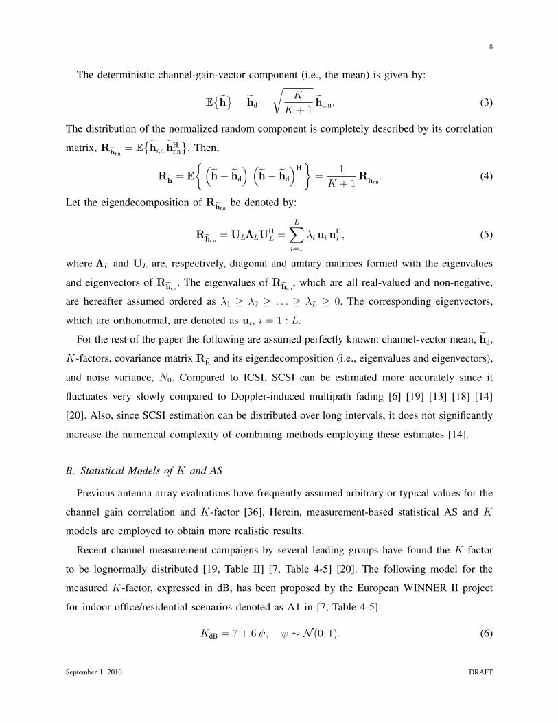
The deterministic channel-gain-vector component (i.e., the mean) is given by:

E{h}= hd =

√K

K + 1hd,n. (3)

The distribution of the normalized random component is completely described by its correlation

matrix, Rhr,n= E

{hr,n h

Hr,n

}. Then,

Rh = E{(

h− hd

) (h− hd

)H}

=1

K + 1Rhr,n

. (4)

Let the eigendecomposition of Rhr,nbe denoted by:

Rhr,n= ULΛΛΛLU

HL =

L∑i=1

λi ui uHi , (5)

where ΛΛΛL and UL are, respectively, diagonal and unitary matrices formed with the eigenvalues

and eigenvectors of Rhr,n. The eigenvalues of Rhr,n

, which are all real-valued and non-negative,

are hereafter assumed ordered as λ1 ≥ λ2 ≥ . . . ≥ λL ≥ 0. The corresponding eigenvectors,

which are orthonormal, are denoted as ui, i = 1 : L.

For the rest of the paper the following are assumed perfectly known: channel-vector mean, hd,

K-factors, covariance matrix Rh and its eigendecomposition (i.e., eigenvalues and eigenvectors),

and noise variance, N0. Compared to ICSI, SCSI can be estimated more accurately since it

fluctuates very slowly compared to Doppler-induced multipath fading [6] [19] [13] [18] [14]

[20]. Also, since SCSI estimation can be distributed over long intervals, it does not significantly

increase the numerical complexity of combining methods employing these estimates [14].

B. Statistical Models of K and AS

Previous antenna array evaluations have frequently assumed arbitrary or typical values for the

channel gain correlation and K-factor [36]. Herein, measurement-based statistical AS and K

models are employed to obtain more realistic results.

Recent channel measurement campaigns by several leading groups have found the K-factor

to be lognormally distributed [19, Table II] [7, Table 4-5] [20]. The following model for the

measured K-factor, expressed in dB, has been proposed by the European WINNER II project

for indoor office/residential scenarios denoted as A1 in [7, Table 4-5]:

KdB = 7 + 6ψ, ψ ∼ N (0, 1). (6)


9

The linear-scale K-factor, i.e., K = 100.1KdB , is then lognormally distributed.

On the other hand, intended-signal power arrives with azimuth angle dispersion that is typically

modeled by the Laplacian power azimuth spectrum (PAS) [12, Section 4.2.1] [15, Chapter 1] [6].

PAS width is characterized by AS, which determines antenna correlation [12, Section 4.2.2] [15,

Chapter 1]. Thus, AS affects the channel eigenvalue magnitudes [13] and eigenvector directions.

Measured base-station AS, expressed in degrees, is lognormally distributed, e.g., [7, Table 4-5]

AS = 101.64+0.31χ, χ ∼ N (0, 1), (7)

for the A1 scenario, which yields AS mean ≈ 50◦ and standard deviation ≈ 30◦.

Note that the AS and K mean and variance are scenario-dependent, as shown in Table II, based

on [7, Table 4-5]. Furthermore, AS and K can exhibit negative, zero, or positive correlation [7].

Measured correlation coefficient ρ between ψ from (6) and χ from (7) is shown in Table II.

The next section derives antenna performance evaluation and adaptation tools that are deployed

in Section IV to measure performance and complexity realistically, i.e., by averaging over the AS

and K distributions, and unrealistically, i.e., by setting AS and K to their distribution averages

(which is the typical approach in the literature).

III. MAXIMAL-RATIO EIGENCOMBINING (MREC)

A. MREC for Perfect ICSI

For completeness of exposition, the main steps of MREC of order N , denoted hereafter as

MRECN , for perfect ICSI are reviewed below from [13, Section III.A.1] [16, Section II.A]:

(1) Let L × N matrix UN△= [u1 u2 . . . uN ] transform the L-dimensional signal vector from

Eqn. (1) into the N -dimensional vector

y =√Es bh+ n, (8)

where

y△= UH

N y, h△= UH

N h, n△= UH

N n. (9)

This is the well-known Karhunen-Loeve transform (KLT). The elements of the N -dimensional

post-KLT vectors y, h, and n are hereafter referred to as eigenbranches, eigengains, and

eigen-noises, respectively.


10

(2) For perfect ICSI, the transformed signal vector is linearly combined, based on the MRC

criterion [36], with

wMREC = h. (10)

Our assumptions about the fading and noise distributions imply that:

• h ∼ Nc(hd,1

K+1ΛΛΛN), where hd

△= UH

N hd =√

KK+1

UHN hd,n, and ΛΛΛN is the diagonal matrix

formed by the first N eigenvalues of Rhr,n; the eigengains hi, i = 1 : L, are uncorrelated

and, thus, independent.

• n ∼ Nc(0, N0 IN); the eigen-noises are uncorrelated and, thus, independent.

• h and n are mutually uncorrelated, and, thus, independent.

The post-KLT channel eigengain vector can be written as

h =

√K

K + 1hd,n +

√1

K + 1hr,n, (11)

where hr,n△= UH

N hr,n. Then, the K-factor for the ith eigenbranch, i.e., the post-KLT ratio of the

powers in the deterministic and the random components of hi is:

Ki =K

K+1|hd,n,i|2

1K+1

E{|hr,n,i|2}= K

|uHi hd,n|2

λi. (12)

The angle ϕi defined by

cosϕi =uHi hd,n

∥ui∥ ∥hd,n∥(13)

characterizes the relative ‘direction’ of hd,n with respect to ui. Since ∥ui∥2 = 1 and ∥hd,n∥2 =

L, (12) becomes:

Ki = K L| cosϕi|2

λi. (14)

The specular component of the channel-gain vector determines transceiver performance through

K and ϕi, i = 1 : N . On the other hand, the diffuse component determines transceiver

performance through the eigenvalue magnitudes (which depend on the AS) [13]. Thus, antenna

performance for Rician fading is determined by both the relative strengths and the relative

‘directions’ of the deterministic and random multipath components [44].


11

B. MREC for Estimated ICSI

Next, we generalize our Rayleigh-fading analysis from [13, Section III.D] to Rician fading.

Although this analysis applies more generally, numerical results are shown in Section IV for

ICSI estimated based on PSAM at the transmitter and pilot-sample interpolation at the receiver

[26] [39] [28]. Suboptimal and optimal PSAM-based ICSI estimation approaches denoted SINC

PSAM and MMSE PSAM, respectively, are described in [11] [12, Section 3.6] [26, Section II.E]

[28, Section II.B] [39, Section II]. Appendix A compares their pre- and post-KLT complexities.

Fig. 1 depicts MREC implementation. The second main step in MRECN requires N eigengain

estimates. Note that MRC requires L gain estimates, and N ≤ L. Its detailed steps are as

follows: 1) for each transmitted symbol, sample the baseband received-signal-vector; 2) for at

most one symbol per channel coherence period [22, p. 15], use the received received-signal-

vector sample to update the channel eigenvalues and eigenvectors [14] [17, p. 1685]; when

these estimates have changed significantly [6] [18] update N , as shown in Section III-F; 3) for

each received-signal-vector sample, perform the KLT; 4) at the pilot symbol in each slot, use the

post-KLT received-signal-vector sample to update the eigengain vector estimate [12, Section 3.6];

5) for each data (i.e., nonpilot) sample combine the post-KLT received signal vector with the

corresponding eigengain vector estimate (as shown in Section III-D below); 6) demodulate the

result to obtain an estimate of the transmitted symbol.

C. Numerical Complexity

Computational complexity refers herein to the number of complex-number multiplications

required per symbol by MREC, BF, and MRC for combining (at symbol-rate), channel gain

or eigengain estimation (at Doppler rate), and eigentructure estimation (much less often [14]).

It has been evaluated in detail in our previous work [13] [14]: ICSI estimation and combining

complexity is shown in [13, Table II]; channel eigenvector and eigenvalue estimation complexity

appears in [14, Table II]. SINC and MMSE PSAM ICSI estimation complexity is also discussed

in Appendix A. Since AS and K vary slowly [7], estimation of the eigenbranch K-factors

from (12) with the method from [20, Section II.B] is accurate and requires little per-symbol

processing. Thus, we assume that Ki, i = 1 : N , are perfectly known and we neglect their

estimation complexity.


12

D. Exact MREC

This section reviews the implementation of optimum MREC given eigengain estimates and

SCSI, based on our previous work for Rayleigh fading [13]. Note that, as mentioned in the

introduction, most previous research has dealt with suboptimum combining. Details on optimum

and suboptimum combining can be found in Appendix B.

Let us assume that the eigengain vector, h, and its estimate, g, are jointly Gaussian (as for

MMSE and SINC PSAM). The mean of g is denoted gd. Then, conditioned on g, the channel

eigengain vector can be factored as [13]

h = m+ e, e ∼ Nc (0,Re) , (15)

with uncorrelated m and e described by [32, Eqns. (5),(6)]

m△= E{h|g} = E{h}+Rhg R

−1g (g − gd) , (16)

Re△= E{(h−m) (h−m)H|g} = Rh −Rhg R

−1g Rgh. (17)

Conditioned on g, the post-KLT signal vector from (8) can be reexpressed as

y =√Es bm+ ννν ∼ Nc(

√Es bm,Rννν), (18)

where m is the effective channel eigengain vector after collecting the channel estimation im-

pairments and noise into the effective eigen-noise vector ννν △=

√Es b e + n, whose correlation

matrix is Rννν = Es Re +N0 IN .

The correlation coefficient of the ith channel eigengain hi and its estimate gi is

µi△=

σhi,gi√σ2hiσ2gi

=

√K + 1

λi

σhi,giσgi

, (19)

where correlations σhi,gi△= E{(hi − hd,i) (gi − gd,i)

∗} and σ2gi

△= E{|gi−gd,i|2} can be computed

for SINC and MMSE PSAM and Rician fading by generalizing the expressions obtained for

Rayleigh fading in [11].

Then, since eigenbranch independence renders the elements of g independent, and the covari-

ance matrices from (15)-(18) diagonal, the elements of m and Rννν are, respectively:

mi = hd,i +σhi,giσ2gi

(gi − gd,i) =

√K

K + 1hd,n,i +

√λi

K + 1µigi − gd,i

σgi(20)

[Rννν ]i,i = Es

(1

K + 1λi −

|σhi,gi|2

σ2gi

)+N0 =

1

K + 1Es λi

(1− |µi|2

)+N0 (21)


13

Given m and Rννν , the weight vector that yields maximum SNR, i.e., the MRC combiner, for

the post-KLT received-signal model in (18) is

we,N = R−1ννν m. (22)

Then, maximum-likelihood detection of the transmitted symbol requires searching for the con-

stellation symbol of minimum distance to the symbol-detection decision variable

wHe,N y =

√Es bw

He,N m+wH

e,N ννν. (23)

Since b is multiplied in (18) by the real-valued factor wHe,N y = mH R−1

ννν m, the symbol error

probability can be written (as shown later in (34) based on [41]), in terms of the effective

symbol-detection SNR

γ =E{|

√Es bw

He,N m|2}

E{|wHe,N ννν|2}

= Es|mH R−1

ννν m|2

E{|mH R−1ννν ννν|2}

= Es mH R−1

ννν m. (24)

Since Rννν is diagonal, this SNR can be written as

γ = Es

N∑i=1

|mi|2

[Rννν ]i,i=

N∑i=1

γi, (25)

i.e., as the sum of the eigenbranch effective SNRs, given by

γi =Es |mi|2

[Rννν ]i,i=

EsN0

∣∣∣∣√K hd,n,i +√λi µi

(gi−gd,i)σgi

∣∣∣∣2EsN0λi (1− |µi|2) +K + 1

. (26)

The average of γi is

Γi =

EsN0

(K∣∣hd,n,i

∣∣2 + λi |µi|2)

EsN0λi (1− |µi|2) +K + 1

=EsN0λi (Ki + |µi|2)

EsN0λi (1− |µi|2) +K + 1

. (27)

Note that more accurate estimation (i.e., a larger |µi|) yields a larger Γi.

Due to the summation property (25), this combining method has been denoted ‘exact’ MREC

[13]. From (22), the exact-MREC weights are

[we,N ]i =mi

[Rννν ]i,i, i = 1 : N. (28)

Note that the conventional weights are, simply,

[wa,N ]i = gi, i = 1 : N. (29)

Exact and approximate combining approaches are compared in Appendix B. For exact combining,

we apply the elegant AEP-derivation procedure from [36, Chapter 9].


14

E. Derivation of Exact-MREC AEP, for Rician Fading

The effective K-factor on the ith eigenbranch of (18), i.e., the ratio of the powers in the

deterministic and the random parts of mi from (20), is:

κi =K

K+1|hd,n,i|2

|µi|2 λiK+1

1σ2gi

E{|gi − gd,i|2

} =K |hd,n,i|2

λi

1

|µi|2= Ki

1

|µi|2≥ Ki. (30)

Then, it can be shown that the eigenbranch SNRs from (26) are independent random variables

each with a noncentral-χ2 distribution described by p.d.f. [36, Eqn. (2.16), p. 21]

p(γi) =(κi + 1) e

−[κi+

(κi+1) γiΓi

]Γi

I0

√4κi (κi + 1) γiΓi

, (31)

where I0 is the zeroth-order modified Bessel function of the first kind. The m.g.f. of γi is [36,

Eqn. (2.17), p. 21]

Mγi(s) = E{es γi} =κi + 1

(κi + 1)− sΓi

eκi sΓi

(κi+1)−sΓi . (32)

Recall from (25) that the exact-MREC symbol-detection SNR is the sum of the individual

SNRs, which are statistically independent. Therefore, the m.g.f. of γ is:

Mγ(s) = E{es γ} =N∏i=1

Mγi(s). (33)

Given the symbol-detection SNR γ, the M -PSK error probability can be written as [41, Eqn. (5)]

[36, Eqn. (8.22)]

Pe,N(γ) =1

π

∫ M−1M

π

0

exp

{−γ gPSK

sin2 ϕ

}dϕ, gPSK = sin2 π

M. (34)

Then, the AEP can be written in terms of the m.g.f. of γ, as follows:

Pe,N△= E{Pe,N(γ)} =

1

π

∫ M−1M

π

0

Mγ

(− gPSK

sin2 ϕ

)dϕ. (35)

Substituting (33) into (35) yields:

Pe,N =1

π

∫ M−1M

π

0

N∏i=1

Mγi

(− gPSK

sin2 ϕ

)dϕ. (36)

Substituting (32) into (36) yields the symbol-AEP expression for exact MRECN in Rician fading:

Pe,N =1

π

∫ M−1M

π

0

N∏i=1

κi + 1

κi + 1 + gPSKsin2 ϕ

Γi

exp

{−

κigPSKsin2 ϕ

Γi

κi + 1 + gPSKsin2 ϕ

Γi

}dϕ. (37)


15

This expression depends on modulation constellation size, M , MREC order, N , antenna correla-

tion (i.e., also AS, through the eigenvalues, λi, i = 1 : N ), fading model (through K), specular

and diffuse component directions (through ϕi), as well as ICSI accuracy. Therefore, (37) is useful

in evaluating the effect of channel features, e.g., AS and K randomness and correlation, and

practical receiver processing, e.g., SINC or MMSE PSAM-based ICSI estimation on performance.

Note that MREC AEP expressions can be derived similarly for other modulations, as mentioned

in Appendix C-8.

Significantly, though not a closed-form, the AEP expression (37) is readily implemented and

quickly evaluated on a computer. With this AEP expression overall performance (averaging over

fading, AS, and K) can be evaluated faster than through the simulation-only approach. Note that

the corresponding AEP expression for Rayleigh fading has been validated against results from

more time-consuming simulations in [12, Figs. 3.16-17].

Finally, Appendix C discusses special cases and generalizations of the above AEP derivation,

e.g., for BF and MRC, perfect ICSI, Rayleigh fading, as well as for MISO and MIMO systems.

F. New Optimum Order Selection Method for MREC

For Rayleigh fading and the received-signal model from (8) we have previously adapted the

MREC order to γb and AS (assuming eigenvalues ordered decreasingly) with the criterion [13]:

minN=1:L

[L∑

i=N+1

Es E{|hi|2}+N∑j=1

E{|nj|2}

]= min

N=1:L

[Es

L∑i=N+1

λi +N0N

]. (38)

This criterion is known as the bias–variance tradeoff criterion (BVTC) [8, Eqns. (15),(16),(18)]

because (38) balances the average loss incurred by removing the weakest (L−N) intended-signal

contributions (i.e., bias, the first term) against the residual-noise contribution (i.e., variance, the

second term). For Rayleigh fading and typical urban macrocell scenarios we found that this

BVTC helps MREC substantially reduce the dimension of the ICSI estimation and combining

problems compared to MRC, i.e., typically N ≪ L [13].

Compared to Rayleigh fading, Rician fading also contributes via the deterministic component

to the average intended-signal power. Therefore, the Rayleigh BVTC from (38) has to be

modified, for Rician fading and the signal model from (8), as follows [43, Eqn. (28)]:

minN=1:L

[L∑

i=N+1

Es E{|hi|2}+N∑j=1

E{|nj|2}

]= min

N=1:L

[Es

L∑i=N+1

(K∣∣hd,n,i

∣∣2K + 1

+λi

K + 1

)+N0N

](39)


16

Substituting Ki from (12), (39) becomes:

minN=1:L

[Es

L∑i=N+1

λiKi + 1

K + 1+N0N

]. (40)

The bias term in (40) is determined by K, ϕi, and λi, i = 1 : L — see also (14). Thus, this BVTC

requires knowing K and reordering, decreasingly, the bias terms, i.e., λi (Ki + 1), i = 1 : L.

Note that, since K fluctuates slowly, its estimation has low complexity and high accuracy [19]

[20].

Since BVTC for Rayleigh and Rician fading from (38) and (40), respectively, are derived for

the signal model from (8), the selected MREC order accounts for the average-bit-SNR, K, as

well as for the AS-dependent ϕi angles in (13). However, since the BVTC from (40) does not

account for ICSI accuracy, it is hereafter denoted as the non-CSI (NCSI) BVTC.

Therefore, we propose a new BVTC, based on the CSI-conditioned signal model in (18):

minN=1:L

[L∑

i=N+1

Es E{|mi|2}+N∑j=1

[Rννν ]j,j

]. (41)

Using (20) and (21) this becomes:

minN=1:L

[Es

L∑i=N+1

(K∣∣hd,n,i

∣∣2K + 1

+λi |µi|2

K + 1

)+

N∑j=1

(Es λj (1− |µj|2)

K + 1+N0

)]. (42)

Substituting (12), (42) becomes:

minN=1:L

[Es

L∑i=N+1

λi

(Ki

K + 1+

|µi|2

K + 1

)+

N∑j=1

(Es λj (1− |µj|2)

K + 1+N0

)]. (43)

Finally, substituting (30), (43) becomes:

minN=1:L

[Es

L∑i=N+1

λi |µi|2κi + 1

K + 1+

N∑j=1

(Es λj (1− |µj|2)

K + 1+N0

)]. (44)

Besides λi and ϕi, i = 1 : L (which are determined by AS and K) this new BVTC also

accounts for ICSI accuracy, through µi, and is therefore denoted as CSI BVTC hereafter. It

reduces to NCSI BVTC from (40) for perfect ICSI, i.e., when µi = 1, i = 1 : L. Note that

λi |µi|2 (κi+1) = λi (Ki + |µi|2), i = 1 : L, should be ordered decreasingly. Now, since |µi| ≤ 1,

ICSI estimation error decreases the bias term and increases the variance term for CSI BVTC (43)

over NCSI BVTC (40). Thus, CSI BVTC yields lower MREC order, i.e., lower processing

complexity, than NCSI BVTC. Notice that, for CSI BVTC, knowledge of µi, i = 1 : L, can be

acquired accurately (mathematically [11] or by estimation) for low complexity, because of slow

channel statistics fluctuation [6] [7].


17

IV. NUMERICAL RESULTS

The derived AEP expression and BVTC are applied to prove the adaptive-MREC effectiveness

in realistic channels, and to evaluate MREC realistically, i.e., by averaging over the AS and K

distributions, as well as unrealistically, i.e., by setting AS and K to their distribution averages.

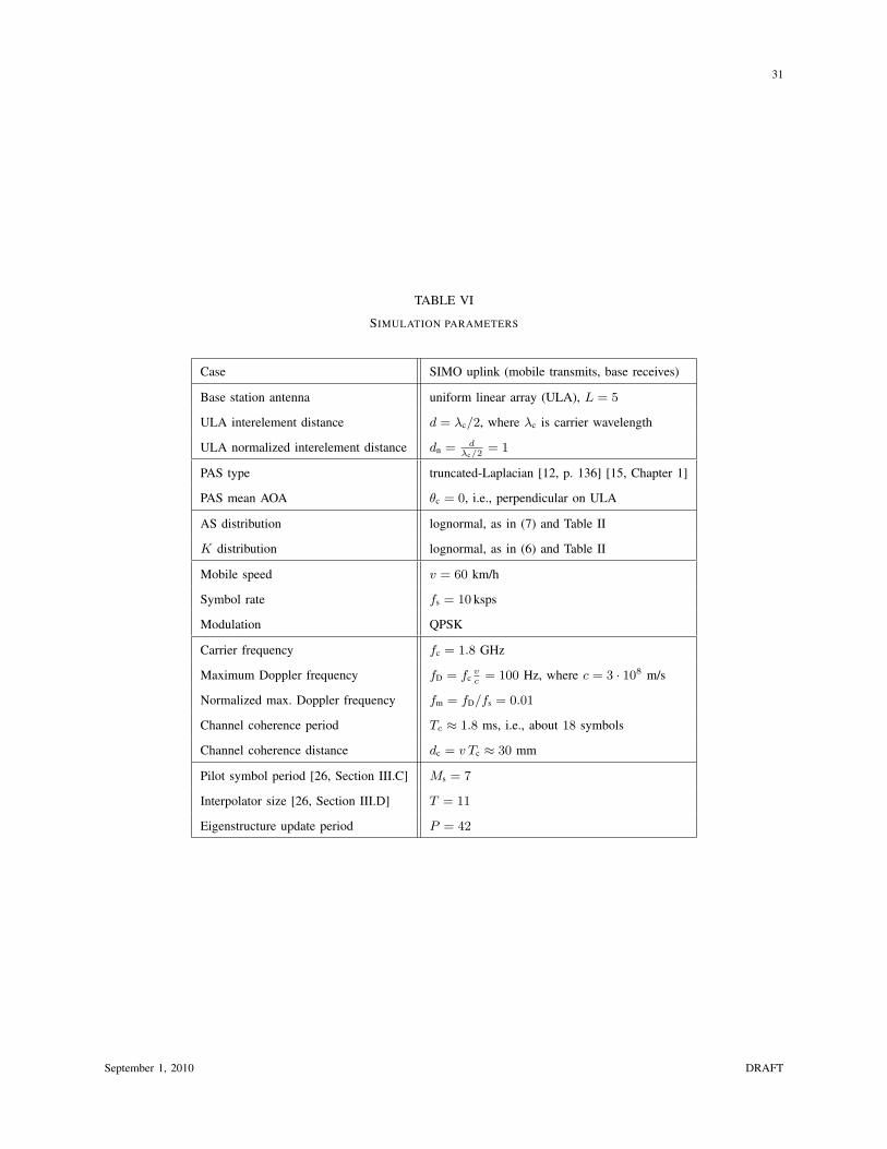
A. Simulation Setup

For numerical results described next the parameter values shown in Table VI and the procedure

described below have been used:

a) A batch of 10 000 independent AS samples is generated from lognormal distributions as

shown in (7) with scenario-dependent parameters from Table II.

b) A corresponding batch of 10 000 independent K samples is generated from lognormal

distributions as shown in (6) with scenario-dependent parameters from Table II, so that

AS and K have the required correlation.

c) At each (AS, K) sample, error probability averaged over the fading is computed with (37).

d) The mean AEP is computed by numerically averaging over AS and K.

We also compute the AEP and complexity for AS and K set to their distribution averages.

B. MRC, BF, and Adaptive MREC Performance and Complexity. Rician Fading, Equal K-factors.

In this subsection the AEP expression in (37) is used to evaluate MREC, MRC, and BF

perfromance, and test the effectiveness of MREC adaptation with the CSI-BVTC proposed

in (44). Let us consider scenario A1, ρ = −0.6, equal K-factors, and MMSE PSAM.

Fig. 2 shows that adaptive MREC underperforms MRC by only about 0.7 dB at mean-AEP

10−3, but is about seven times less complex. This dramatic complexity reduction for MMSE

PSAM is mainly due to the KLT, as explained in Appendix A.

The complexity of MREC over MRC is also reduced by the BVTC. Fig. 2 shows that, while

MREC performance degrades with lower bit-SNR, MREC complexity relative to that of MRC

also decreases. This is because the BVTC output decreases, as lower SNR lowers the BVTC

bias term. On the other hand, MRC performance degrades but complexity remains the same.

Fig. 2 also indicates that BVTC-based adaptation and diversity gain help MREC outperform

BF by nearly 8 dB at mean-AEP 10−3, although at the cost of substantially higher complexity.


18

These results obtained with our AEP expression and new CSI BVTC confirm that, for Rician

fading, adaptive MREC is more efficient than MRC and more effective than BF.

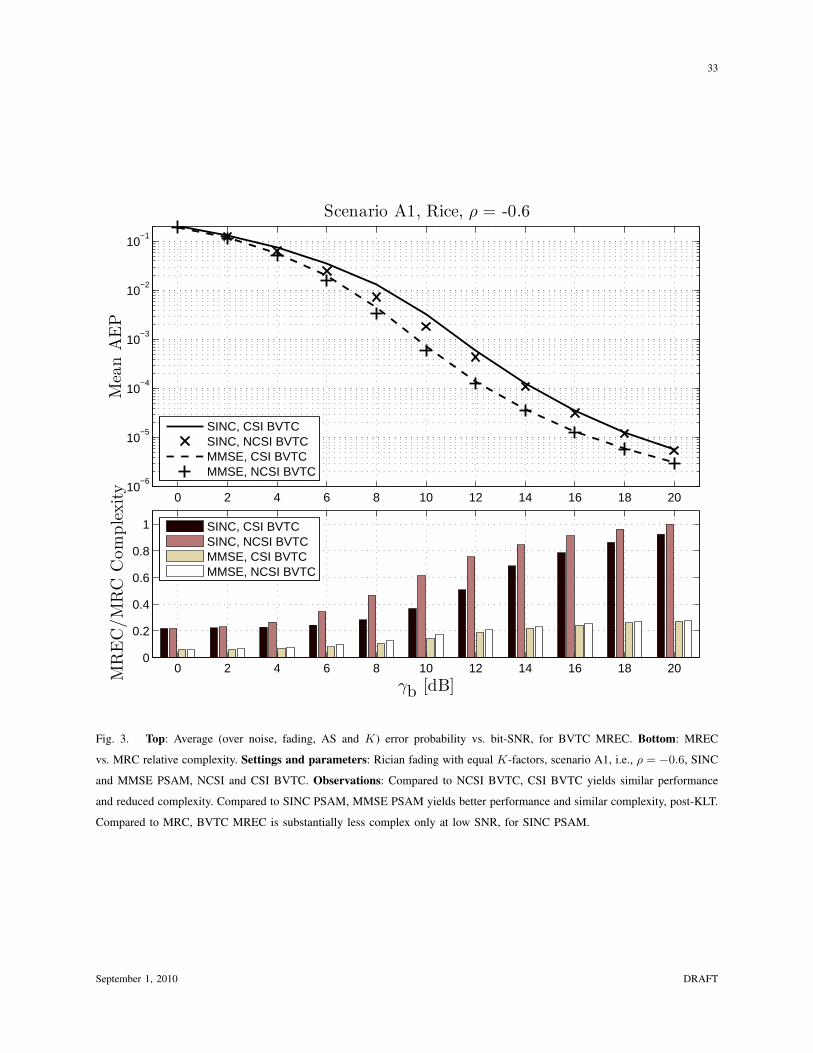
C. CSI vs. NCSI BVTC Performance and Complexity

Next, the derived AEP expression is used to compare the conventional and proposed BVTCs,

and SINC and MMSE PSAM. Let us consider scenario A1, ρ = −0.6, and equal K-factors.

Fig. 3 shows that for both MMSE and SINC PSAM, MREC adapted with NCSI BVTC (40)

only very slightly outperforms MREC adapted with CSI BVTC (44) at relevant performance

levels (e.g., for mean-AEP lower than 10−3). Over the shown SNR range, for SINC PSAM,

NCSI BVTC MREC outperforms CSI BVTC MREC by less than 1 dB but can be 40% more

complex. On the other hand, for MMSE PSAM, NCSI BVTC MREC can outperform CSI BVTC

MREC by less than 0.3 dB but can be 15% more complex. Thus, the CSI BVTC derived for

MREC that is optimum given ICSI estimate and SCSI is more effective for MREC adaptation.

D. SINC vs. MMSE PSAM Performance and Complexity

Fig. 3 also shows, in the top subplot, that MMSE PSAM outperforms SINC PSAM by almost

2 dB at mean AEP 10−3. Therefore, MREC with MMSE PSAM should be deployed because

post-KLT MMSE and SINC PSAM have similar complexity, as explained in Appendix A.

On the other hand, for MRC, pre-KLT MMSE PSAM is exceedingly complex compared to

SINC PSAM, as explained in Appendix A. Therefore, the MREC vs. MRC relative complexity

is much lower for MMSE compared to SINC PSAM, as the bottom subplot indicates.

Finally, the bottom subplot indicates that, for SINC PSAM, MREC is much less complex than

MRC only at low SNR (unlike for MMSE PSAM, where MREC is much less complex than

MRC throughout the SNR range). This is because: 1) pre- and post-KLT SINC PSAM have

similar complexities; 2) only at low SNR the BVTC can significantly reduce the dimension of

the estimation and combining procedures.

E. Performance and Complexity for All Scenarios

Here, the newly-derived MREC analysis and adaptation tools are employed for a wide range

of scenarios for which measurement-based fading parameter models are available. Thus, CSI

BVTC MREC evaluation results for all scenarios from Table II are reported.


19

Fig. 4 shows, in the top subplot, the SNR required to achieve mean-AEP 10−3, and in the

bottom subplot the corresponding MREC vs. MRC relative complexity. The groups of bars

correspond to scenarios (identified on the abscissa, as in Table II), whereas the bars in each

group correspond to fading models (in the order identified by text at the top of the figure).

Let us first examine the effects of fading models conventionally employed in theoretical

analyses. Rayleigh fading (indicated by dash-dotted line) demands the highest SNR and numerical

complexity, whereas Rician fading with mean K (indicated by dashed line) tends to require low

SNR and complexity. For the measurement-supported distributions and correlations of K and

AS shown in Table II (indicated by solid line), performance and complexity fall between those

for Rayleigh and mean-K Rician fading. Furthermore, higher |ρ| demands lower SNR (outdoor

scenarios incur larger differences) for slightly higher complexity.

For the measured scenario A1 (Rician fading, ρ = −0.6, E{KdB} = 7 dB) adaptive MREC

requires 1.8 dB lower SNR and 52% lower complexity than those expected for the Rayleigh

fading model (K = 0, AS random). Furthermore, for the Rician fading model with KdB = 7 dB

(and AS random) adaptive MREC requires very slightly lower SNR and 33% lower complexity

than those expected for the measured scenario A1.

For scenario B1 (Rician fading, ρ = −0.3, E{KdB} = 9 dB) adaptive MREC requires 4.8 dB

lower SNR and 43% lower complexity than those expected for the Rayleigh fading model.

Furthermore, for the Rician fading model with KdB = 9 dB adaptive MREC requires 4.9 dB

lower SNR and 27% lower complexity than those expected for the measured scenario B1.

Scenarios B3, C1, and C2 are not evaluated because their measured ρ is positive and small.

Herein, we have focused on the negative values for ρ because they are supported by theoretical

analysis [45] and because measured |ρ| are then higher — see Table II.

For scenarios D1 and D2a (ρ = 0, E{KdB} = 7 dB) adaptive MREC requires 1.8 − 2.3 dB

lower SNR and 37− 38% lower complexity than those expected for the Rayleigh fading model.

Furthermore, for the Rician fading model with KdB = 7 dB adaptive MREC requires 2.3−2.6 dB

lower SNR and 19− 22% lower complexity than those expected for the measured scenarios D1

and D2a.

Thus, the newly-derived AEP expression (37) and CSI-BVTC (44) are effective for perfor-

mance evaluation and adaptation, respectively, in all scenarios described in Table II.


20

F. Explanation of MREC Performance Dependence on |ρ|

Small AS implies small diversity gain. Low K implies weak specular component. Thus, MREC

AEP (averaging over noise and fading only) is highest for low AS and K values. Then, the (low-

AS, low-K) samples dominate performance averaged over AS and K. Thus, the relative number

of such samples is important. Histograms obtained numerically for (AS, K) have indicated

that, for ρ < 0, increasing |ρ| yields relatively fewer (low-AS, low-K) samples. This means

relatively fewer worst-performance-inducing samples and, so, improved average (over AS and

K) performance, as revealed in the top subplot of Fig. 4.

G. MRC, BF, and Adaptive MREC Performance and Complexity. Rician Fading, Unequal Ks.

As mentioned in the introduction, fixed wireless links can experience unequal branch K-factors

[46] [38]. The MREC AEP expression from (37) is then still applicable after changes discussed

in Appendix D. On the other hand, the CSI BVTC derived for unequal K-factors in (54) in

Appendix D is used herein. As an example, let us evaluate comparatively MRC, BF, and CSI-

BVTC MREC for scenario A1 (ρ = −0.6, E{KdB} = 7 dB) unequal branch K-factors, and

MMSE PSAM. Recall that results for similar settings but equal K-factors have been presented

in Section IV-B.

Fig. 5 depicts the performance and complexity of MRC, BF, and adaptive MREC. The AS

sequence is generated as explained in Section IV-A, using the lognormal distribution from (7).

Then, L mutually independent K-factor sequences (i.e., one for each branch) is generated as

explained in Section IV-A, using the lognormal distribution from (6). The AEP is computed

with (37) for each (AS, K1, K2, . . . , KL) sample. Finally, the AEP samples are averaged.

Comparing the results for unequal K-factors from Fig. 5 with those for equal K-factors from

Fig. 2 reveals that BF performs much worse (4 dB, at mean-AEP 2 · 10−3) for unequal vs. equal

K-factors, whereas MRC performs somewhat better for unequal vs. equal K-factors (especially

at high SNR). Thus, besides AS-induced diversity, MRC also benefits from K-factor diversity.

On the other hand, neither AS-induced diversity nor K diversity benefits BF. Finally, CSI BVTC

MREC yields MRC-like performance also for unequal K-factors at mean-AEP near 10−3, but

has higher complexity than for equal K-factors. The effect of unequal K-factors is currently

under further investigation.


21

V. CONCLUSIONS

The paper has studied the AEP performance and numerical complexity expected in realistic

channels for a SIMO combining approach that is optimum given ICSI estimate and SCSI.

Combining implementation and analysis is simplified by the KLT decorrelating property. An

AEP expression has thus been derived for estimated and correlated Rician fading for optimum

MREC, MRC, and BF. Significantly, the newly-derived AEP expression is widely applicable

(Rayleigh or Rician fading, equal or unequal K-factors) and is easily averaged numerically

over K-factor and AS distributions. Furthermore, we have proposed a new BVTC for MREC

adaptation to channel condition that, unlike previous results, also accounts for ICSI accuracy.

First, our numerical results confirm that adaptive post-KLT combining (i.e., eigencombining)

can achieve optimum performance for much lower numerical complexity than conventional pre-

KLT combining. Computational savings are especially significant for optimum ICSI estimation.

Therefore, optimum ICSI estimation and adaptive optimum eigencombining should be deployed

alongside for best performance and lowest hardware requirements and power consumption.

Second, the fading type and fading parameter models employed in theoretical analysis or

numerical simulation are shown to dramatically impact performance indications and complex-

ity assessments. For more realistic multi-antenna technology evaluations we recommend using

recently-developed measurement-based Rician fading models with random and correlated AS

and K. Using the Rayleigh fading model instead can lead to substantial MREC performance

underestimation and complexity overestimation. On the other hand, the Rician fading model with

K fixed to typical value can seriously overestimate performance and underestimate complexity.

This knowledge should be useful to system designers.

APPENDIX A

PRE/POST-KLT SINC AND MMSE PSAM COMPLEXITY

Table III reviews ICSI estimate computation requirements for pre-KLT and post-KLT SINC

and MMSE PSAM, based on [12, Section 3.6] [28]. Since pre-KLT MMSE PSAM accounts

for channel gain correlation (by using dimension-LT matrix–vector multiplication), it is much

more complex than post-KLT MMSE PSAM as well as than pre-KLT and post-KLT SINC PSAM

(which use only dimension-T vector inner-product). Table IV details complexity, based on [13,

Table II] [14, Table II]. Therein, P represents the period (in symbols) between samples used


22

for channel eigenstructure (i.e., SCSI) estimation [14]. Note that P must exceed the Doppler-

induced coherence period in order to ensure SCSI estimation based on independent channel

samples. However, P should not exceed the channel stationarity period (determined by AS,

K fluctuation rate). We have found that since P is typically large compared to L and N ,

eigenstructure estimation does not add significantly to MREC complexity [14].

APPENDIX B

EIGEN/COMBINING: IDEAL, APPROXIMATE, AND EXACT

A. Implementation Procedure. Performance

Table V depicts combining methods: 1) ideal combining, i.e., for perfect ICSI; 2) approximate

combining given ICSI estimates; 3) exact combining given ICSI estimates as well as channel and

noise statistics. Table IV shows their numerical complexity. Given the channel and noise statistics,

the practice of multiplying the signal vector only with the ICSI estimate is, in general, suboptimal

[30] [31] [13] [12] [33]. We have therefore denoted this approach ‘approximate’ eigen/combining.

Though exact MREC (described in Section III-D) performs better than approximate MREC

(described and analyzed in [13] [12, Section 3.7.2]), as shown in [12, Section 3.7.3] [31] [33],

they require similar numerical complexities, as noticeable from Table IV. Finally, exact MRC

[12, Appendix A] [31] is more complex than approximate MRC [27] [35] [39] [28] [29].

Now, the KLT is an orthonormal and linear transformation. Combining is also a linear trans-

formation. Therefore, for perfect ICSI, MRC and MRECL yield the same symbol-detection

SNR, i.e., they are performance-equivalent [25]. Furthermore, SINC and MMSE PSAM are

linear procedures. Furthermore, both exact and approximate combining are linear procedures.

Thus, MRC and MRECL have been found to be performance-equivalent for both exact and

approximate combining [13, Section III.D.2] [12, Section 3.9.3]. Therefore, the performance of

MRECN approaches that of MRC as the MREC order N increases.

B. Analysis Procedure

Approximate-MRC analysis has been a difficult problem, typically tackled based on the

symbol-detection decision variable [27] [35] [39] [28] [29]. Difficulties introduced by channel

correlation in approximate-MRC analysis can be avoided based on the performance-equivalence

between MRC and MRECL. On the other hand, exact combining analysis is substantially simpler


23

than for approximate combining because the former is based on the symbol-detection SNR which

has the remarkable property from (25). Finally, for i.i.d. channel gains, exact combining can be

shown to reduce to approximate combining. Thus, exact-combining analysis results (which can

be obtained more easily) are applicable to approximate combining [13, Section 3.11.4].

APPENDIX C

MREC-ANALYSIS SPECIAL CASES AND GENERALIZATIONS

1) BF: For N = 1, exact MREC becomes BF, and then (37) is the BF AEP expression. This

SIMO statistical beamforming method corresponds to the one-dimensional statistical beamform-

ing method for MISO from [17] and for MIMO from [18].

2) MRC: As explained in Appendix B-A, MRC and MRECL are performance-equivalent.

Therefore, (37) for MRECL also describes exact-MRC performance for Rician fading. Recall

from Appendix B that exact-MRC implementation is cumbersome and analysis can be difficult

through means other than this relationship with exact MREC [31] [12, Appendix A].

3) Ideal MREC: Perfect ICSI implies: gi = hi, hd,i = gd,i, σhi,gi = σ2gi

= σ2hi

= 1K+1

λi,

µi = 1, mi = hi, κi = Ki, [Rννν ]i,i = N0, [we,N ]i = hi, γi = EsN0

|hi|2, and Γi =EsN0λi. Substituting

these into (37) yields the ideal-MREC AEP [47, Eqn. (15)].

4) Exact-MREC for Rayleigh Fading: Then, (37) can be shown to reduce to [13, Eqn. (28)].

5) Exact-MREC for Rayleigh I.I.D. Fading: KLT is redundant. On the other hand, in (20)

and (21), hd,i, gd,i, λi, σgi , µi, and [Rννν ]i,i are the same ∀i = 1 : L. For Rayleigh fading, mi

from (20) reduces to mi =σh,gσ2ggi. If σh,g is real-valued and positive (as for SINC and MMSE

PSAM [11] [12, p. 83]), then (28) and (29) yield wHe,N y = wH

a,N y. Thus, a simple approximate-

MRC AEP expression for i.i.d. Rayleigh fading follows from (37) and (27), for E{|hl|2} = 1

[40, Eqn. (23)] [13, Section III.E.1]:

Pe,L =1

π

∫ M−1M

π

0

[1 +

gPSK

sin2 ϕ

Es |µ|2

Es (1− |µ|2) +N0

]−L

dϕ, (45)

which can be expressed in closed-form as in [16, Appendix, Eqn. (33)].

6) Exact-MRC for Rician I.I.D. Fading and Simpler ICSI Model: Wu et al. [32] have derived

an exact-MRC AEP expression starting with the distribution of the true ICSI given its estimate

[32, Eqns. (5),(6)], which here is described by (16) and (17). However, they have made the follow-

ing limiting assumptions: i.i.d. channel gains, E{g} = E{h} [32, Eqn. (6a)], and h = g+e [32,


24

Eqn. (3)]. Our derivations, based on [30], apply for independent and nonidentically-distributed

channel gains, E{g} = E{h}, and any jointly-Gaussian ICSI and estimate. Furthermore, our

results apply for MRC of correlated branches, through MREC.

7) Generalizations: For Rician fading and correlated channel gains, the principles of our

SIMO exact eigencombining analysis can also be applied to MISO and MIMO systems with

symbol-detection SNR writable as a sum of uncorrelated random variables with noncentral-χ2

distributions, as in (25), by following the decorrelation procedure from [36, p. 440] [25] [17,

Eqns. (4)-(8)], e.g., for: 1) MISO with transmitter ICSI estimate and perfect SCSI, i.e., for exact

maximum-ratio transmission; 2) MISO and MIMO with receiver ICSI estimate, e.g., Alamouti

and other orthogonal space-time block coding [22, Sections 5.4.1, 5.4.3]; an exact-combining-

like procedure is analyzed for Rayleigh i.i.d. channel gains in [42]; 3) MISO with transmit SCSI

and receiver perfect ICSI, i.e., two-dimensional statistical eigenbeamforming [17, Eqn. (9)] [18].

8) Other Modulations: Note that the symbol-error probability can be expressed in terms of the

symbol-detection SNR similarly to (34) also for other modulations, e.g., multiple amplitude-shift-

keying (M-ASK), multiple-amplitude modulation (M-AM), and quadrature-amplitude modulation

(QAM) [36, Chapter 8]. Then, the straightforward approach from Section III-E can yield easy-

to-compute AEP expressions.

APPENDIX D

THE CASE OF UNEQUAL K-FACTORS

When K-factors are different on different branches [21], i.e., Kl, l = 1 : L, the lth element

of the channel gain vector can be factored as

hl =

√Kl

Kl + 1hd,n,l +

√1

Kl + 1hr,n,l, (46)

but the entire channel gain vector can no longer be factored as in (2). Therefore, we now use

instead the generic Rician-fading channel-gain-vector model

h = hd + hr, (47)

so that h ∼ Nc(hd,Rh), where Rh = E{hr h

Hr

}= ULΛΛΛLU

HL =

∑Li=1 λi ui u

Hi .

Eqn. (4) shows that, when Kl = K, ∀l = 1 : L, Rh is a multiplication of two terms: a

scalar that depends on K, and a matrix that depends on spatial correlation. For unequal Kls,


25

such factorization is not possible. Then, the eigenvalues and eigenvectors of Rh incorporate

information about all K-factors.

The post-KLT received eigen-signal vector conditioned on the channel-eigengain-vector esti-

mate is described by (15)-(17). However, for unequal Kl, the elements of m and Rννν are now:

mi = hd,i +√λi µi

gi − gd,i

σgi, (48)

[Rννν ]i,i = Es λi(1− |µi|2

)+N0. (49)

Thus, for the ith eigenbranch, the effective SNR is now given by

γi =Es |mi|2

[Rννν ]i,i=

EsN0

∣∣∣∣hd,i +√λi µi

gi−gd,iσgi

∣∣∣∣2EsN0λi (1− |µi|2) + 1

, (50)

which has noncentral-χ2 distribution with average

Γi =

EsN0

(∣∣hd,i∣∣2 + λi |µi|2

)EsN0λi (1− |µi|2) + 1

. (51)

On the other hand, the effective K-factor for the ith eigenbranch is now:

κi =|hd,i|2

λi

1

|µi|2. (52)

The AEP-derivation approach from Section III-E leads for unequal K-factors to the same AEP

expression as for equal K-factors, i.e., Eqn. (37). Nonetheless, Γi and κi should now be computed

with (51) and (52), respectively.

Finally, for unequal K-factors, the NCSI BVTC from (39) becomes:

minN=1:L

[Es

L∑i=N+1

(|hd,i|2 + λi

)+N0N

], (53)

whereas the CSI BVTC from (44) becomes:

minN=1:L

[Es

L∑i=N+1

(|hd,i|2 + λi |µi|2

)+

N∑j=1

[Es λj (1− |µj|2) +N0

]]. (54)


26

REFERENCES

[1] D. G. Brennan, “Linear diversity combining techniques,” Proc. of the IEEE, vol. 91, no. 2, pp. 331 – 356, February 2003.

[2] S. Applebaum, “Adaptive arrays,” IEEE Trans. on Ant. and Propag., vol. 24, no. 5, pp. 585 – 598, September 1976.

[3] R. A. Monzingo and T. W. Miller, Introduction to Adaptive Arrays. New York: John Wiley and Sons, 1980.

[4] A. J. Paulraj, D. A. Gore, R. U. Nabar, and H. Bolcskei, “An overview of MIMO communications - a key to gigabit

wireless,” Proc. of the IEEE, vol. 92, no. 2, pp. 198 – 218, February 2004.

[5] D. Gesbert, M. Kountouris, R. Heath, C.-B. Chae, and T. Salzer, “Shifting the MIMO paradigm,” IEEE Signal Processing

Magazine, vol. 24, no. 5, pp. 36 –46, Sep. 2007.

[6] A. Algans, K. I. Pedersen, and P. E. Mogensen, “Experimental analysis of the joint statistical properties of azimuth spread,

delay spread, and shadow fading,” IEEE Journal on Sel. Areas in Comm., vol. 20, no. 3, pp. 523–531, April 2002.

[7] P. Kyosti, J. Meinila, L. Hentila, and et al., “WINNER II Channel Models.” CEC, Tech. Rep. IST-4-027756, 2008.

[8] F. Dietrich and W. Utschick, “On the effective spatio-temporal rank of wireless communication channels,” in Proc. 13th

IEEE Int. Symp. on Personal, Indoor and Mobile Radio Communications, (PIMRC ’02), vol. 5, 2002, pp. 1982–1986.

[9] J. Choi and S. Choi, “Diversity gain for CDMA systems equipped with antenna arrays,” IEEE Trans. on Veh. Tech., vol. 52,

no. 3, pp. 720–725, May 2003.

[10] F. A. Dietrich and W. Utschick, “Maximum ratio combining of correlated Rayleigh fading channels with imperfectly known

channel,” IEEE Comm. Lett., vol. 7, no. 9, pp. 419–421, September 2003.

[11] C. Siriteanu and S. D. Blostein, “Maximal-ratio eigencombining: a performance analysis,” Canadian Journal of Electrical

and Computer Engineering, vol. 29, no. 1/2, pp. 15–22, January–April 2004.

[12] C. Siriteanu, “Maximal-ratio eigen-combining for smarter antenna array wireless communication receivers,” Ph.D.

dissertation, Queen’s University, Kingston, Canada, 2006.

[13] C. Siriteanu and S. D. Blostein, “Maximal-ratio eigen-combining for smarter antenna arrays,” IEEE Trans. on Wireless

Comm., vol. 6, no. 3, pp. 917 – 925, March 2007.

[14] C. Siriteanu, G. Xin, and S. D. Blostein, “Performance and complexity comparison of MRC and PASTd-based statistical

beamforming and eigencombining,” in Proc. 14th Asia–Pacific Conf. on Communications (APCC’08), Tokyo, Japan, Session

16-PM1-A, 2008.

[15] C. Sun, J. Cheng, and T. Ohira, Eds., Handbook on Advancements in Smart Antenna Technologies for Wireless Networks.

Chapter ‘Eigencombining: A Unified Approach to Antenna Array Signal Processing’ by C. Siriteanu and S. D. Blostein.

New York, NY: Idea Group, Inc., 2009.

[16] C. Siriteanu and S. D. Blostein, “Performance and complexity analysis of eigencombining, statistical beamforming, and

maximal-ratio combining,” IEEE Trans. on Veh. Tech., vol. 58, no. 7, pp. 3383 – 3395, September 2009.

[17] S. Zhou and G. B. Giannakis, “Optimal transmitter eigen-beamforming and space-time block coding based on channel

correlations,” IEEE Trans. on Information Theory, vol. 49, no. 7, pp. 1673 – 1690, July 2003.

[18] H. Sampath, V. Erceg, and A. Paulraj, “Performance analysis of linear precoding based on field trials results of MIMO-

OFDM system,” IEEE Trans. on Wireless Comm., vol. 4, no. 2, pp. 404–409, March 2005.

[19] V. Erceg, P. Soma, D. S. Baum, and S. Catreux, “Multiple-input multiple-output fixed wireless radio channel measurements

and modeling using dual-polarized antennas at 2.5 GHz,” IEEE Trans. on Wireless Comm., vol. 3, no. 6, pp. 2288 – 2298,

November 2004.

[20] L. J. Greenstein, S. S. Ghassemzadeh, V. Erceg, and D. G. Michelson, “Ricean K-factors in narrow-band fixed wireless

channels: Theory, experiments, and statistical models,” IEEE Trans. on Veh. Tech., vol. 58, no. 8, pp. 4000 – 4012, 2009.


27

[21] R. Valenzuela, L. Ahumada, and R. Feick, “The effect of unbalanced branches on the performance of diversity receivers

for urban fixed wireless links,” IEEE Trans. on Wireless Comm., vol. 6, no. 9, pp. 3324–3332, September 2007.

[22] A. J. Paulraj, R. U. Nabar, and D. A. Gore, Introduction to Space-Time Wireless Communications. Cambridge, UK:

Cambridge University Press, 2005.

[23] S. Choi, J. Choi, H.-J. Im, and B. Choi, “A novel adaptive beamforming algorithm for antenna array CDMA systems with

strong interferers,” IEEE Trans. on Veh. Tech., vol. 51, no. 5, pp. 808–816, September 2002.

[24] R. Vaughan and J. B. Andersen, Channels, Propagation and Antennas for Mobile Communications. London, UK: The

Institution of Electrical Engineers, 2003.

[25] X. Dong and N. C. Beaulieu, “Optimal maximal ratio combining with correlated diversity branches,” IEEE Comm. Lett.,

vol. 6, no. 1, pp. 22–24, January 2002.

[26] J. K. Cavers, “An analysis of pilot symbol assisted modulation for Rayleigh fading channels,” IEEE Trans. on Veh. Tech.,

vol. 40, no. 4, pp. 686 – 693, November 1991.

[27] X. Dong and N. C. Beaulieu, “SER of two-dimensional signalings in Rayleigh fading with channel estimation errors,” in

IEEE Int. Conf. on Communications, (ICC ’03), vol. 4, 11-15 2003, pp. 2763 – 2767 vol.4.

[28] Y. Ma, R. Schober, and D. Zhang, “Exact BER for M-QAM with MRC and imperfect channel estimation in Rician fading

channels,” IEEE Trans. on Wireless Comm., vol. 6, no. 3, pp. 926 –936, March 2007.

[29] R. Annavajjala, P. Cosman, and L. Milstein, “Performance analysis of linear modulation schemes with generalized diversity

combining on Rayleigh fading channels with noisy channel estimates,” IEEE Trans. on Information Theory, vol. 53, no. 12,

pp. 4701 –4727, Dec. 2007.

[30] P. Polydorou and P. Ho, “Error performance of M-PSK with diversity combining in non-uniform Rayleigh fading and

non-ideal channel estimation,” in Proc. IEEE Veh. Tech. Conf., (VTC ’00), vol. 1, 2000, pp. 627 – 631.

[31] D. K. Shamain and L. B. Milstein, “Detection with spatial diversity using noisy channel estimates in a correlated fading

channel,” in Proc. IEEE Military Communications Conf., (MILCOM ’02), vol. 1, 2002, pp. 691 – 696.

[32] J. Wu, C. Xiao, and N. C. Beaulieu, “Optimal diversity combining based on noisy channel estimation,” in IEEE Int. Conf.

on Communications, (ICC’ 04), vol. 1, 2004, pp. 214 – 218.

[33] Y. Chen and N. C. Beaulieu, “Novel diversity receivers in the presence of Gaussian channel estimation errors,” IEEE

Trans. on Wireless Comm., vol. 5, no. 8, pp. 2022 –2025, Aug. 2006.

[34] Y. Ma, R. Schober, and S. Pasupathy, “Effect of channel estimation errors on MRC diversity in Rician fading channels,”

IEEE Trans. on Veh. Tech., vol. 54, no. 6, pp. 2137–2142, November 2005.

[35] R. Annavajjala, “A simple approach to error probability with binary signaling over generalized fading channels with

maximal ratio combining and noisy channel estimates,” IEEE Trans. on Wireless Comm., vol. 4, no. 2, pp. 380–383,

March 2005.

[36] M. K. Simon and M.-S. Alouini, Digital Communication Over Fading Channels. A Unified Approach to Performance

Analysis. Baltimore, Maryland: John Wiley and Sons, 2000.

[37] Q. H. Spencer, B. D. Jeffs, M. A. Jensen, and A. L. Swindlehurst, “Modeling the statistical time and angle of arrival

characteristics of an indoor multipath channel,” IEEE Journal on Sel. Areas in Comm., vol. 18, no. 3, pp. 347–360, March

2000.

[38] L. Ahumada, R. Feick, R. Valenzuela, and C. Morales, “Measurement and characterization of the temporal behavior of

fixed wireless links,” IEEE Trans. on Veh. Tech., vol. 54, no. 6, pp. 1913 – 1922, Nov. 2005.


28

[39] L. Cao and N. C. Beaulieu, “Closed-form BER results for MRC diversity with channel estimation errors in Ricean fading

channels,” IEEE Trans. on Wireless Comm., vol. 4, no. 4, pp. 1440–1447, July 2005.

[40] R. Annavajjala and L. B. Milstein, “Performance analysis of linear diversity-combining schemes on Rayleigh fading

channels with binary signaling and Gaussian weighting errors,” IEEE Trans. on Wireless Comm., vol. 4, no. 5, pp. 2267–

2278, September 2005.

[41] J. W. Craig, “A new, simple and exact result for calculating the probability of error for two-dimensional signal

constellations,” in Proc. IEEE Military Communications Conf., (MILCOM ’91), vol. 2, 1991, pp. 571 – 575.

[42] W. Li and N. C. Beaulieu, “Effects of channel-estimation errors on receiver selection-combining schemes for Alamouti

MIMO systems with BPSK,” IEEE Trans. on Comm., vol. 54, no. 1, pp. 169 – 178, Jan. 2006.

[43] C. Siriteanu, Y. Miyanaga, and S. D. Blostein, “Smart antenna performance and complexity for correlated azimuth spread

and Rician K-factor,” in Int. Conf. on Green Circuits and Systems, Shanghai, China, (ICGCS’10), June 2010.

[44] R. U. Nabar, H. Bolcskei, and A. J. Paulraj, “Diversity and outage performance in space-time block coded Ricean MIMO

channels,” IEEE Trans. on Wireless Comm., vol. 4, no. 5, pp. 2519 – 2532, September 2005.

[45] G. D. Durgin and T. S. Rappaport, “Theory of multipath shape factors for small-scale fading wireless channels,” IEEE

Trans. on Ant. and Propag., vol. 48, no. 5, pp. 682 – 693, May 2000.

[46] R. Valenzuela, L. Ahumada, R. Feick, and S. Gysling, “Temporal fade reduction for fixed wireless diversity receivers with

unbalanced and correlated branches,” IEEE Comm. Lett., vol. 11, no. 2, pp. 129 –131, Feb. 2007.

[47] C. Siriteanu, Y. Miyanaga, and S. D. Blostein, “Smart antenna performance for correlated azimuth spread and Rician

K-factor,” in Proc. 4th Int. Symp. on Communications, Control and Signal Processing, Limassol, Cyprus, (ISCCSP’10),

March 2010.


29

TABLE I

ACRONYMS

Acronym Term

Information

CSI Channel state information

ICSI Instantaneous CSI

SCSI Statistical CSI

Combining

MREC Maximal-ratio eigencombining

MRC Maximal-ratio combining

BF Statistical beamforming

Estimation

PSAM Pilot-symbol-aided modulation

SINC Sinc-function interpolation

MMSE Minimum mean-square-error interpolation

Transform KLT Karhunen-Loeve transform

Order selection

BVTC Bias-variance tradeoff criterion

CSI-BVTC BVTC considering ICSI accuracy

NCSI-BVTC BVTC disregarding ICSI accuracy

AzimuthPAS Power azimuth spectrum

AS Azimuth spread

Performance AEP Average error probability

TABLE II

BASE-STATION AS AND K STATISTICS FOR LOS SCENARIOS [7, TABLE 4-5]

Code Scenario AS [◦] K ρ

A1 indoor office/residential 101.64+0.31χ 100.1(7+6ψ) −0.6

B1 typical urban microcell 100.40+0.37χ 100.1(9+6ψ) −0.3

B3 large indoor hall 101.22+0.18χ 100.1(2+3ψ) +0.2

C1 suburban 100.78+0.12χ 100.1(9+7ψ) +0.2

C2 typical urban macrocell 101.00+0.25χ 100.1(7+3ψ) +0.1

D1 rural macrocell 100.78+0.21χ 100.1(7+6ψ) +0.0

D2a rural, high-speed 100.70+0.31χ 100.1(7+6ψ) +0.0


30

TABLE III

ICSI ESTIMATION

SINC PSAM MMSE PSAM

Pre-KLTCorrelation Disregarded Considered

Computation Inner product, [11, Eqn. (42)] [12, p. 83] Matrix–vector product [12, p. 83] [28]

Post-KLTCorrelation 0 0

Computation Inner product Inner product

TABLE IV

NUMERICAL COMPLEXITY

Combining Interpolation MRC MRECN

ApproximateSINC L (T + 1) N (L+ T + 1) + 4LN/P

MMSE L (LT + 1) N (L+ T + 1) + 4LN/P

ExactSINC L (L+ T + 1) N (L+ T + 2) + 4LN/P

MMSE L (LT + L+ 1) N (L+ T + 2) + 4LN/P

TABLE V

EIGEN/COMBINING IMPLEMENTATION

Method MRC MREC

Ideal hH y [1] hH y [15, Chapter 1]

Approximate gH y [27] [35] [39] [28] [29] gH y [13]

Exact [12, Appendix A] [31] wHe,N y

��

��

��

��

��

� �

��

��

��

��

��

�

��

Fig. 1. MREC implementation diagram


31

TABLE VI

SIMULATION PARAMETERS

Case SIMO uplink (mobile transmits, base receives)

Base station antenna uniform linear array (ULA), L = 5

ULA interelement distance d = λc/2, where λc is carrier wavelength

ULA normalized interelement distance dn = dλc/2

= 1

PAS type truncated-Laplacian [12, p. 136] [15, Chapter 1]

PAS mean AOA θc = 0, i.e., perpendicular on ULA

AS distribution lognormal, as in (7) and Table II

K distribution lognormal, as in (6) and Table II

Mobile speed v = 60 km/h

Symbol rate fs = 10 ksps

Modulation QPSK

Carrier frequency fc = 1.8 GHz

Maximum Doppler frequency fD = fcvc= 100 Hz, where c = 3 · 108 m/s

Normalized max. Doppler frequency fm = fD/fs = 0.01

Channel coherence period Tc ≈ 1.8 ms, i.e., about 18 symbols

Channel coherence distance dc = v Tc ≈ 30 mm

Pilot symbol period [26, Section III.C] Ms = 7

Interpolator size [26, Section III.D] T = 11

Eigenstructure update period P = 42


32

0 2 4 6 8 10 12 14 16 18 2010

−6

10−5

10−4

10−3

10−2

10−1

Mea

nA

EP

Scenario A1, Rice, ρ = -0.6, MMSE, CSI BVTC

BFBVTC MRECMRC

0 2 4 6 8 10 12 14 16 18 200

0.2

0.4

0.6

0.8

1

γb [dB]

Rel

ative

Com

ple

xity

BF/MRECMREC/MRC

Fig. 2. Top: Average (over noise, fading, AS and K) error probability vs. bit-SNR, for BF, CSI BVTC MREC, and MRC.

Bottom: BF vs. MREC and MREC vs. MRC relative complexities. Settings and parameters: Rician fading with equal K-

factors, scenario A1, i.e., ρ = −0.6, MMSE PSAM, CSI BVTC. Observations: Compared to MRC, adaptive MREC yields

similar performance and requires much lower complexity.


33

0 2 4 6 8 10 12 14 16 18 2010

−6

10−5

10−4

10−3

10−2

10−1

Mea

nA

EP

Scenario A1, Rice, ρ = -0.6

SINC, CSI BVTCSINC, NCSI BVTCMMSE, CSI BVTCMMSE, NCSI BVTC

0 2 4 6 8 10 12 14 16 18 200

0.2

0.4

0.6

0.8

1

γb [dB]

MR

EC

/M

RC

Com

ple

xity

SINC, CSI BVTCSINC, NCSI BVTCMMSE, CSI BVTCMMSE, NCSI BVTC

Fig. 3. Top: Average (over noise, fading, AS and K) error probability vs. bit-SNR, for BVTC MREC. Bottom: MREC

vs. MRC relative complexity. Settings and parameters: Rician fading with equal K-factors, scenario A1, i.e., ρ = −0.6, SINC

and MMSE PSAM, NCSI and CSI BVTC. Observations: Compared to NCSI BVTC, CSI BVTC yields similar performance

and reduced complexity. Compared to SINC PSAM, MMSE PSAM yields better performance and similar complexity, post-KLT.

Compared to MRC, BVTC MREC is substantially less complex only at low SNR, for SINC PSAM.


34

10

12

14

16

18

20

22

γb

[dB

]

mean-AEP 10−3

Rayleigh; Rice ρ = 0; Rice ρ = −0.3; Rice ρ = −0.6; Rice ρ = −1; Rice K = mean

A1 B1 B3 C1 C2 D1 D2a0

0.05

0.1

0.15

0.2

0.25

MR

EC

/M

RC

Com

ple

xity

Measurement

Theory:Rayleigh

Theory:RicianmeanK

Fig. 4. Top: SNR required to achieve mean-AEP 10−3. Bottom: MREC/MRC complexity required to achieve mean-AEP

10−3. All scenarios, all fading models. Solid-line arrows indicate performance and complexity for measurement-based fading

models. Dashed-line arrows indicate performance and complexity for Rician fading with mean K. Dash-dotted-line arrows

indicate performance and complexity for Rayleigh fading. Settings and parameters: Equal K-factors, MMSE PSAM, CSI

BVTC. Observations: Performance and complexity averaged over K can be much different than for average or zero K.


35

0 2 4 6 8 10 12 14 16 18 20

10−6

10−5

10−4

10−3

10−2

10−1

Mea

n A

EP

Scenario A1, Rice, ρ = -0.6, MMSE, CSI BVTC

BFBVTC MRECMRC

0 2 4 6 8 10 12 14 16 18 200

0.2

0.4

0.6

0.8

1

γb [dB]

Rel

ativ

e C

ompl

exity

BF/MRECMREC/MRC

Fig. 5. Top: Average (over noise, fading, AS and K) error probability vs. bit-SNR, for BF, CSI BVTC MREC, and MRC.

Bottom: BF vs. MREC and MREC vs. MRC relative complexities. Settings and parameters: Rician fading with unequal

K-factors, scenario A1, i.e., ρ = −0.6, MMSE PSAM, CSI BVTC. AEP expression (37) is used, with Γi and κi computed

with (51) and (52), respectively. CSI BVTC (54) is used. Observations: Compared to MRC, adaptive MREC yields similar

performance and requires much lower complexity.


1 Evaluation of Optimum SIMO Combining for Estimated and...

Documents

Transcript of 1 Evaluation of Optimum SIMO Combining for Estimated and...