1 Divide-and-Conquer Approach Lecture 05 Asst. Prof. Dr. Bunyarit Uyyanonvara IT Program, Image and...
102
1 Divide-and-Conquer Approach Lecture 05 Asst. Prof. Dr. Bunyarit Uyyanonvara Asst. Prof. Dr. Bunyarit Uyyanonvara IT Program, Image and Vision Computing Lab. School of Information and Computer Technology Sirindhorn International Institute of Technology Thammasat University http://www.siit.tu.ac.th/bunyarit [email protected] 02 5013505 X 2005 ITS033 – Programming & Algorithms
-
Upload
alice-hunt -
Category
Documents
-
view
213 -
download
1
Transcript of 1 Divide-and-Conquer Approach Lecture 05 Asst. Prof. Dr. Bunyarit Uyyanonvara IT Program, Image and...

1
Divide-and-Conquer Approach
Lecture 05
Asst. Prof. Dr. Bunyarit UyyanonvaraAsst. Prof. Dr. Bunyarit UyyanonvaraIT Program, Image and Vision Computing Lab.
School of Information and Computer Technology
Sirindhorn International Institute of Technology
Thammasat Universityhttp://www.siit.tu.ac.th/bunyarit
[email protected] 5013505 X 2005
ITS033 – Programming & Algorithms

2
ITS033Topic 01Topic 01 -- Problems & Algorithmic Problem SolvingProblems & Algorithmic Problem SolvingTopic 02Topic 02 – Algorithm Representation & Efficiency Analysis – Algorithm Representation & Efficiency AnalysisTopic 03Topic 03 - State Space of a problem - State Space of a problemTopic 04Topic 04 - Brute Force Algorithm - Brute Force AlgorithmTopic 05 - Divide and ConquerTopic 05 - Divide and ConquerTopic 06Topic 06 -- Decrease and ConquerDecrease and ConquerTopic 07Topic 07 - Dynamics Programming - Dynamics ProgrammingTopic 08Topic 08 -- Transform and ConquerTransform and ConquerTopic 09Topic 09 - Graph Algorithms - Graph AlgorithmsTopic 10Topic 10 - Minimum Spanning Tree - Minimum Spanning TreeTopic 11Topic 11 - Shortest Path Problem - Shortest Path ProblemTopic 12Topic 12 - Coping with the Limitations of Algorithms Power - Coping with the Limitations of Algorithms Power
http://www.siit.tu.ac.th/bunyarit/its033.phphttp://www.siit.tu.ac.th/bunyarit/its033.phpand and http://www.vcharkarn.com/vlesson/showlesson.php?lessonid=7http://www.vcharkarn.com/vlesson/showlesson.php?lessonid=7
3
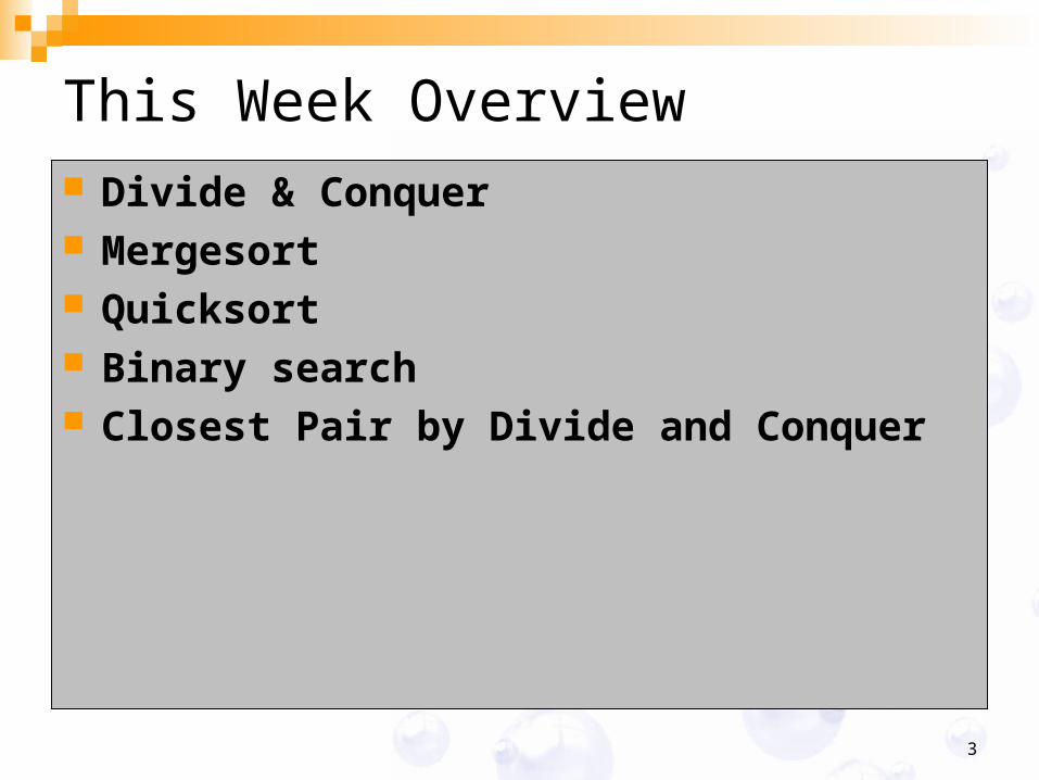
This Week Overview Divide & Conquer Mergesort Quicksort Binary search Closest Pair by Divide and Conquer

4
Divide & Conquer: Introduction
Lecture 05.0
Asst. Prof. Dr. Bunyarit UyyanonvaraAsst. Prof. Dr. Bunyarit UyyanonvaraIT Program, Image and Vision Computing Lab.
School of Information and Computer Technology
Sirindhorn International Institute of Technology
Thammasat Universityhttp://www.siit.tu.ac.th/bunyarit
[email protected] 5013505 X 2005
ITS033 – Programming & Algorithms
5
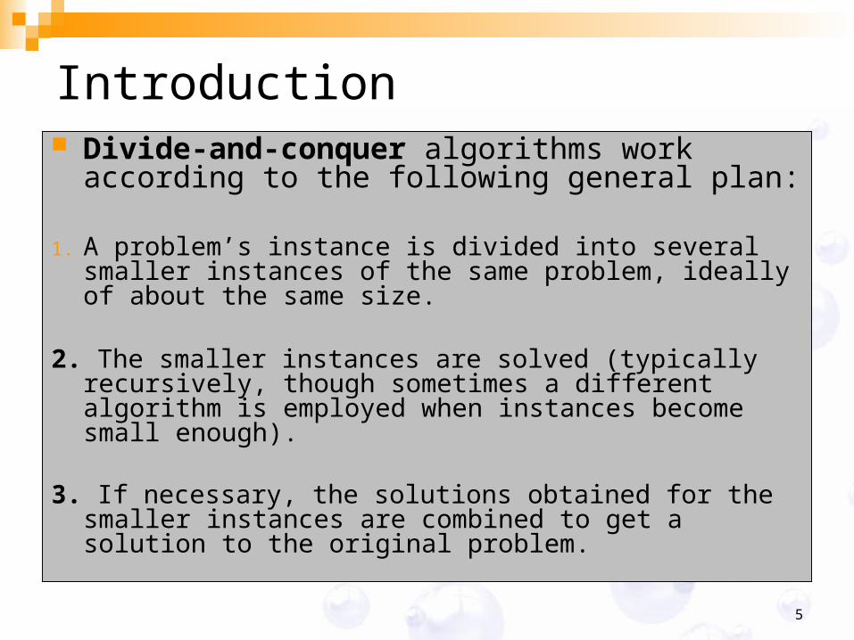
Introduction Divide-and-conquer algorithms work
according to the following general plan:
1. A problem’s instance is divided into several smaller instances of the same problem, ideally of about the same size.
2. The smaller instances are solved (typically recursively, though sometimes a different algorithm is employed when instances become small enough).
3. If necessary, the solutions obtained for the smaller instances are combined to get a solution to the original problem.
6
Divide-and-Conquer
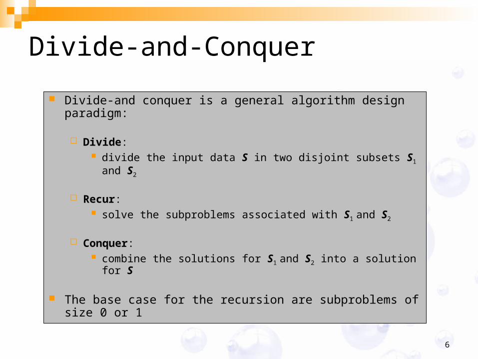
Divide-and conquer is a general algorithm design paradigm:
Divide: divide the input data S in two disjoint subsets S1 and S2
Recur: solve the subproblems associated with S1 and S2
Conquer: combine the solutions for S1 and S2 into a solution for S
The base case for the recursion are subproblems of size 0 or 1
7
Introduction
8
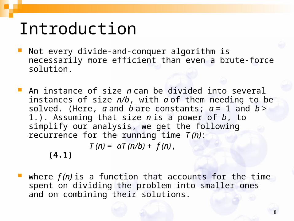
Introduction Not every divide-and-conquer algorithm is necessarily
more efficient than even a brute-force solution.
An instance of size n can be divided into several instances of size n/b, with a of them needing to be solved. (Here, a and b are constants; a = 1 and b > 1.). Assuming that size n is a power of b, to simplify our analysis, we get the following recurrence for the running time T (n):
T (n) = aT (n/b) + f (n), (4.1)
where f (n) is a function that accounts for the time spent on dividing the problem into smaller ones and on combining their solutions.
9
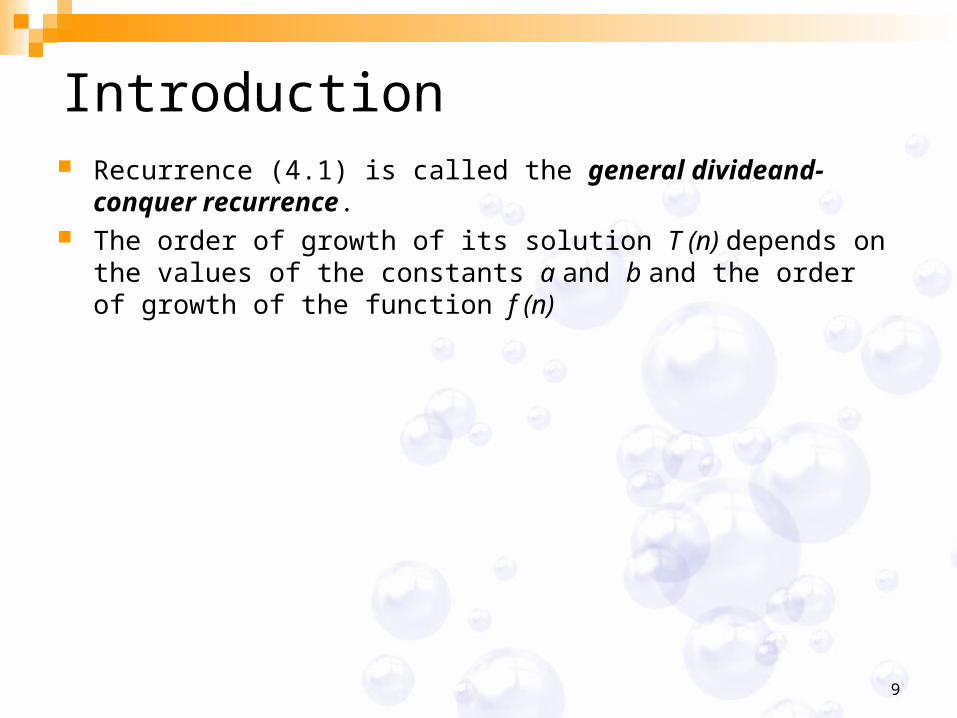
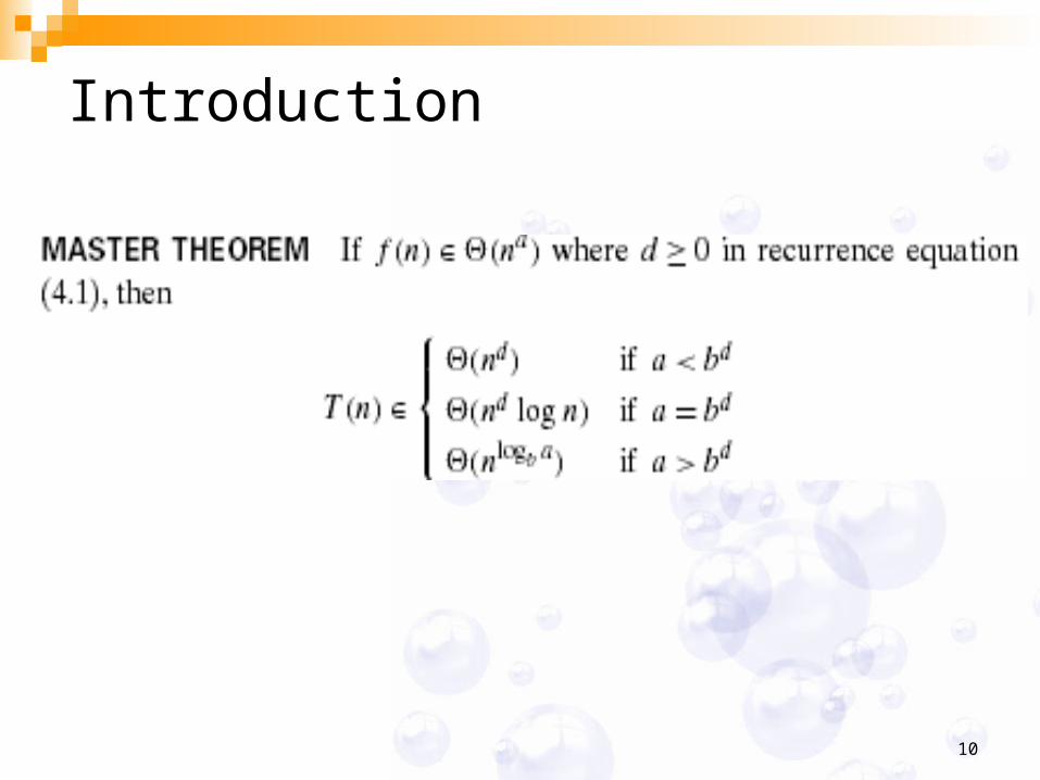
Introduction Recurrence (4.1) is called the general divideand-
conquer recurrence. The order of growth of its solution T (n) depends on the
values of the constants a and b and the order of growth of the function f (n)
10
Introduction
11
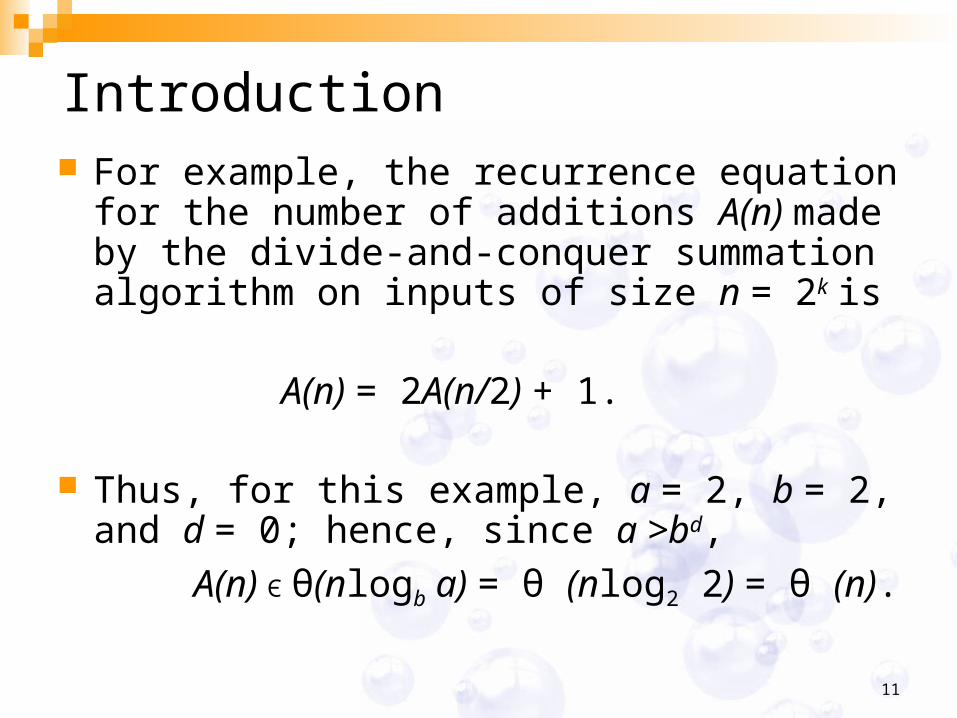
Introduction For example, the recurrence equation for
the number of additions A(n) made by the divide-and-conquer summation algorithm on inputs of size n = 2k is
A(n) = 2A(n/2) + 1.
Thus, for this example, a = 2, b = 2, and d = 0; hence, since a >bd,
A(n) Є θ(nlogb a) = θ (nlog2 2) = θ (n).
12
Advantages
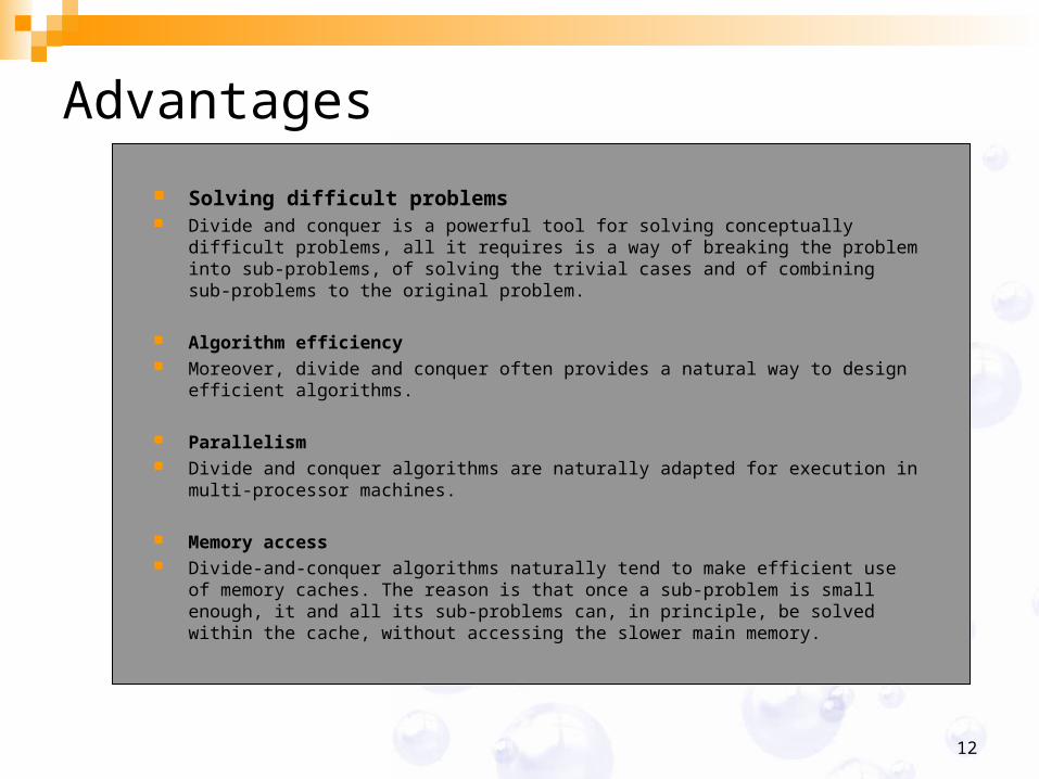
Solving difficult problems Divide and conquer is a powerful tool for solving conceptually difficult problems, all it
requires is a way of breaking the problem into sub-problems, of solving the trivial cases and of combining sub-problems to the original problem.
Algorithm efficiency Moreover, divide and conquer often provides a natural way to design efficient
algorithms.
Parallelism Divide and conquer algorithms are naturally adapted for execution in multi-processor
machines.
Memory access Divide-and-conquer algorithms naturally tend to make efficient use of memory
caches. The reason is that once a sub-problem is small enough, it and all its sub-problems can, in principle, be solved within the cache, without accessing the slower main memory.

13
Divide & Conquer: Mergesort
Lecture 05.1
Asst. Prof. Dr. Bunyarit UyyanonvaraAsst. Prof. Dr. Bunyarit UyyanonvaraIT Program, Image and Vision Computing Lab.
School of Information and Computer Technology
Sirindhorn International Institute of Technology
Thammasat Universityhttp://www.siit.tu.ac.th/bunyarit
[email protected] 5013505 X 2005
ITS033 – Programming & Algorithms

14
IntroductionIntroduction
Sorting is the process of arranging a list of items into Sorting is the process of arranging a list of items into a particular ordera particular order
There must be some values on which the order is There must be some values on which the order is basedbased
There are many algorithms for sorting a list of itemsThere are many algorithms for sorting a list of items
These algorithms vary in efficiencyThese algorithms vary in efficiency
15
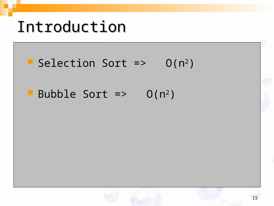
IntroductionIntroduction
Selection Sort => O(nSelection Sort => O(n22))
Bubble Sort => O(nBubble Sort => O(n22))
16
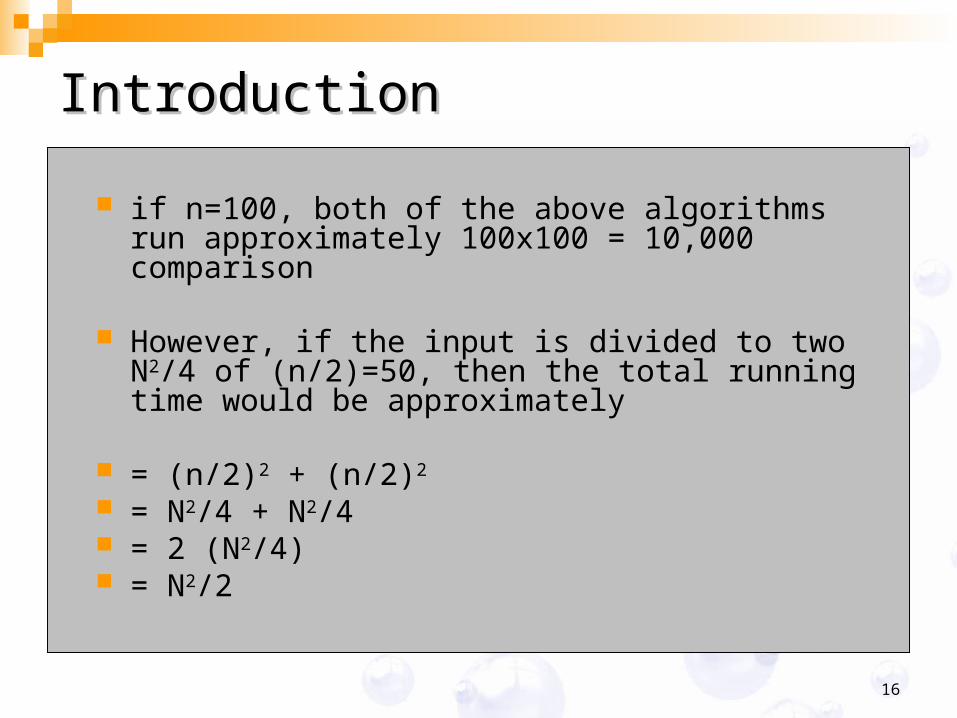
IntroductionIntroduction
if n=100, both of the above algorithms run if n=100, both of the above algorithms run approximately 100x100 = 10,000 approximately 100x100 = 10,000 comparisoncomparison
However, if the input is divided to two NHowever, if the input is divided to two N22/4 of /4 of (n/2)=50, then the total running time would (n/2)=50, then the total running time would be approximately be approximately
= (n/2)= (n/2)22 + (n/2) + (n/2)22 = N= N22/4 /4 + + NN22/4 /4 = 2 (= 2 (NN22/4)/4) = = NN22/2/2

17
Merge Sortthe algorithm
• The strategy behind Merge Sort is to The strategy behind Merge Sort is to change the change the problemproblem of sorting of sorting into the problem of merginginto the problem of merging two two sorted sub-lists into one.sorted sub-lists into one.
• If the two halves of the array were sorted, then merging If the two halves of the array were sorted, then merging them carefully could complete the sort of the entire list.them carefully could complete the sort of the entire list.
18
Merge-Sort
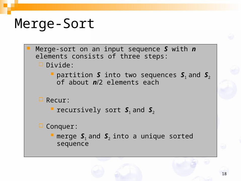
Merge-sort on an input sequence S with n elements consists of three steps: Divide:
partition S into two sequences S1 and S2 of about n2 elements each
Recur: recursively sort S1 and S2
Conquer: merge S1 and S2 into a unique sorted sequence
19
Merge-Sort
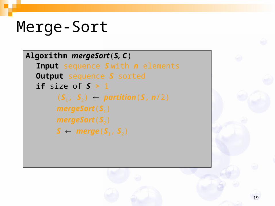
Algorithm mergeSort(S, C)Input sequence S with n elementsOutput sequence S sortedif size of S > 1
(S1, S2) partition(S, n/2)
mergeSort(S1)
mergeSort(S2)
S merge(S1, S2)
20
4 Merge Sortthe algorithm
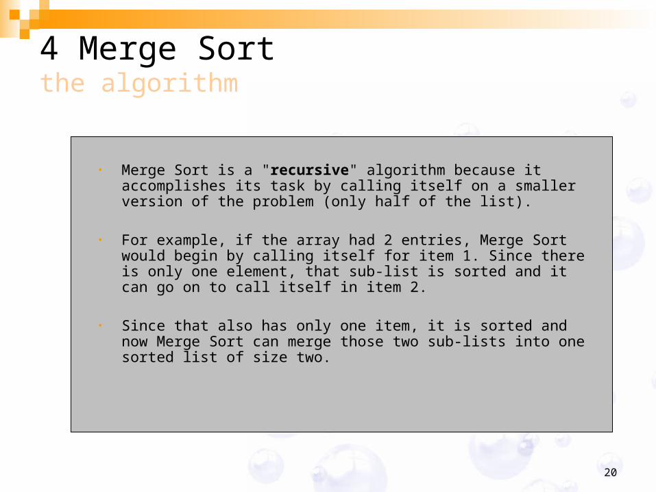
• Merge Sort is a "Merge Sort is a "recursiverecursive" algorithm because it accomplishes its task " algorithm because it accomplishes its task by calling itself on a smaller version of the problem (only half of the list). by calling itself on a smaller version of the problem (only half of the list).
• For example, if the array had 2 entries, Merge Sort would begin by For example, if the array had 2 entries, Merge Sort would begin by calling itself for item 1. Since there is only one element, that sub-list is calling itself for item 1. Since there is only one element, that sub-list is sorted and it can go on to call itself in item 2. sorted and it can go on to call itself in item 2.
• Since that also has only one item, it is sorted and now Merge Sort can Since that also has only one item, it is sorted and now Merge Sort can merge those two sub-lists into one sorted list of size two.merge those two sub-lists into one sorted list of size two.
21
Merging Two Sorted Sequences
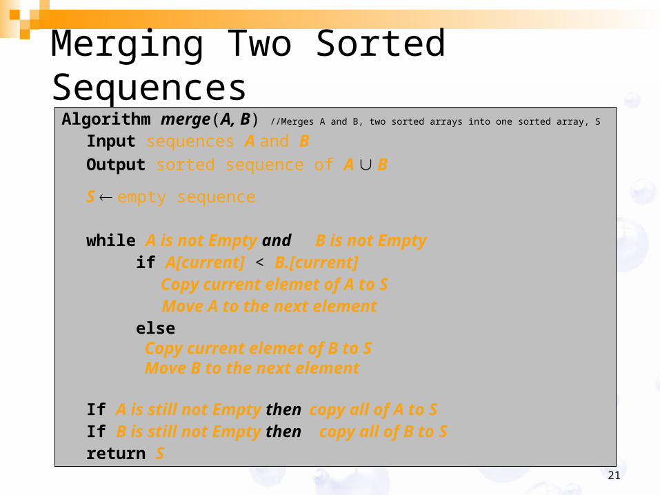
Algorithm merge(A, B) //Merges A and B, two sorted arrays into one sorted array, S
Input sequences A and B
Output sorted sequence of A B
S empty sequence
while A is not Empty and B is not Emptyif A[current] < B.[current]
Copy current elemet of A to S Move A to the next elementelse Copy current elemet of B to S Move B to the next element
If A is still not Empty then copy all of A to SIf B is still not Empty then copy all of B to Sreturn S
22
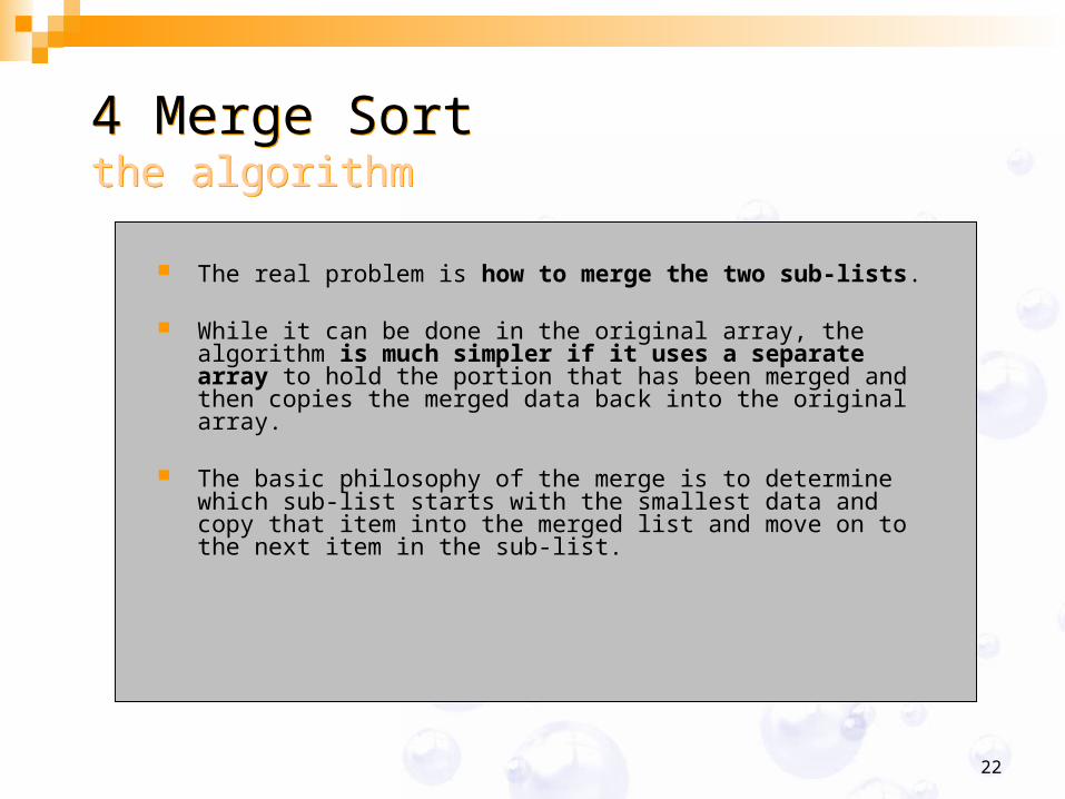
The real problem is The real problem is how to merge the two sub-listshow to merge the two sub-lists. .
While it can be done in the original array, the algorithm While it can be done in the original array, the algorithm is much is much simpler if it uses a separate arraysimpler if it uses a separate array to hold the portion that has been to hold the portion that has been merged and then copies the merged data back into the original array. merged and then copies the merged data back into the original array.
The basic philosophy of the merge is to determine which sub-list starts The basic philosophy of the merge is to determine which sub-list starts with the smallest data and copy that item into the merged list and with the smallest data and copy that item into the merged list and move on to the next item in the sub-list.move on to the next item in the sub-list.
4 Merge Sortthe algorithm4 Merge Sortthe algorithm
23
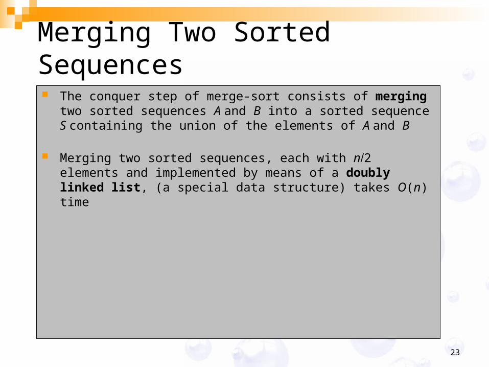
Merging Two Sorted Sequences The conquer step of merge-sort consists of merging two
sorted sequences A and B into a sorted sequence S containing the union of the elements of A and B
Merging two sorted sequences, each with n2 elements and implemented by means of a doubly linked list, (a special data structure) takes O(n) time
24
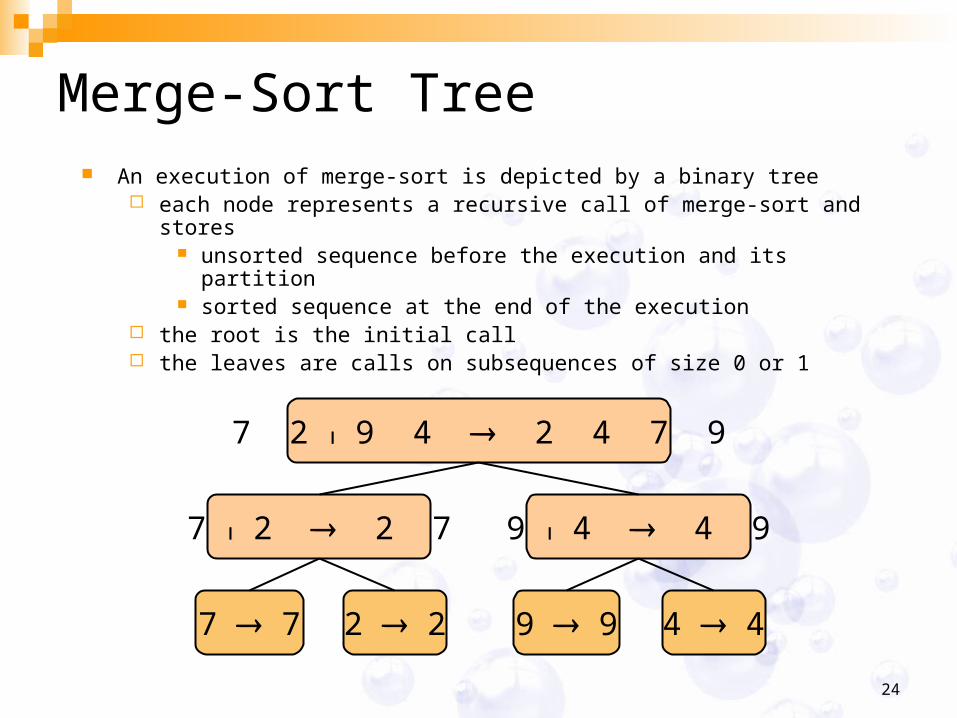
Merge-Sort Tree An execution of merge-sort is depicted by a binary tree
each node represents a recursive call of merge-sort and stores unsorted sequence before the execution and its partition sorted sequence at the end of the execution
the root is the initial call the leaves are calls on subsequences of size 0 or 1
7 2 9 4 2 4 7 9
7 2 2 7 9 4 4 9
7 7 2 2 9 9 4 4
25
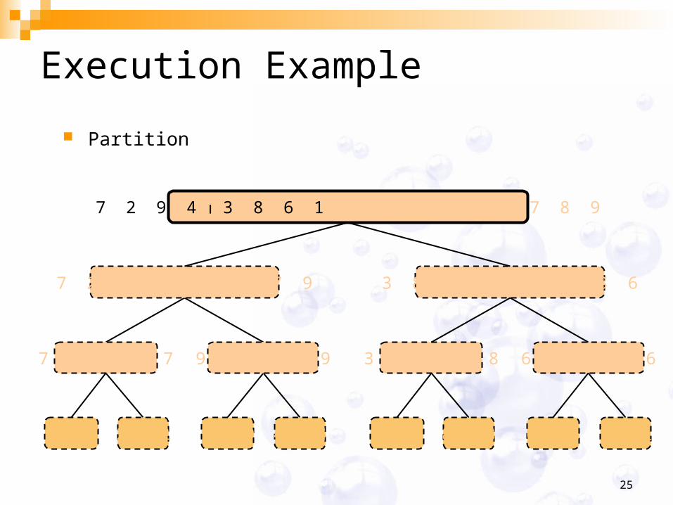
Execution Example
Partition
7 2 9 4 2 4 7 9 3 8 6 1 1 3 8 6
7 2 2 7 9 4 4 9 3 8 3 8 6 1 1 6
7 7 2 2 9 9 4 4 3 3 8 8 6 6 1 1
7 2 9 4 3 8 6 1 1 2 3 4 6 7 8 9
26
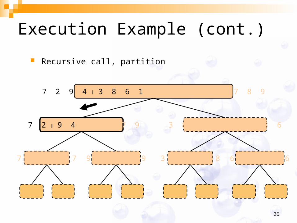
Execution Example (cont.)
Recursive call, partition
7 2 9 4 2 4 7 9 3 8 6 1 1 3 8 6
7 2 2 7 9 4 4 9 3 8 3 8 6 1 1 6
7 7 2 2 9 9 4 4 3 3 8 8 6 6 1 1
7 2 9 4 3 8 6 1 1 2 3 4 6 7 8 9
27
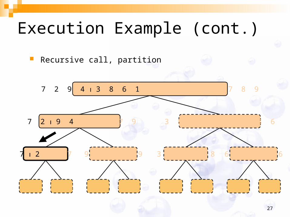
Execution Example (cont.)
Recursive call, partition
7 2 9 4 2 4 7 9 3 8 6 1 1 3 8 6
7 2 2 7 9 4 4 9 3 8 3 8 6 1 1 6
7 7 2 2 9 9 4 4 3 3 8 8 6 6 1 1
7 2 9 4 3 8 6 1 1 2 3 4 6 7 8 9
28
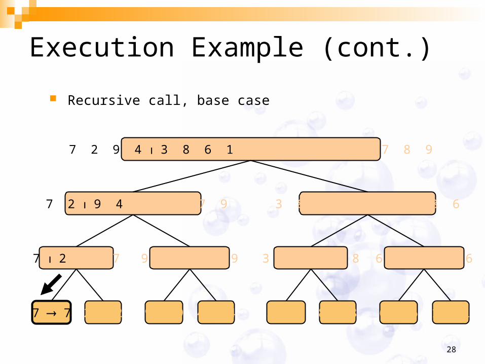
Execution Example (cont.)
Recursive call, base case
7 2 9 4 2 4 7 9 3 8 6 1 1 3 8 6
7 2 2 7 9 4 4 9 3 8 3 8 6 1 1 6
7 7 2 2 9 9 4 4 3 3 8 8 6 6 1 1
7 2 9 4 3 8 6 1 1 2 3 4 6 7 8 9

29
Execution Example (cont.)
Recursive call, base case
7 2 9 4 2 4 7 9 3 8 6 1 1 3 8 6
7 2 2 7 9 4 4 9 3 8 3 8 6 1 1 6
7 7 2 2 9 9 4 4 3 3 8 8 6 6 1 1
7 2 9 4 3 8 6 1 1 2 3 4 6 7 8 9
30
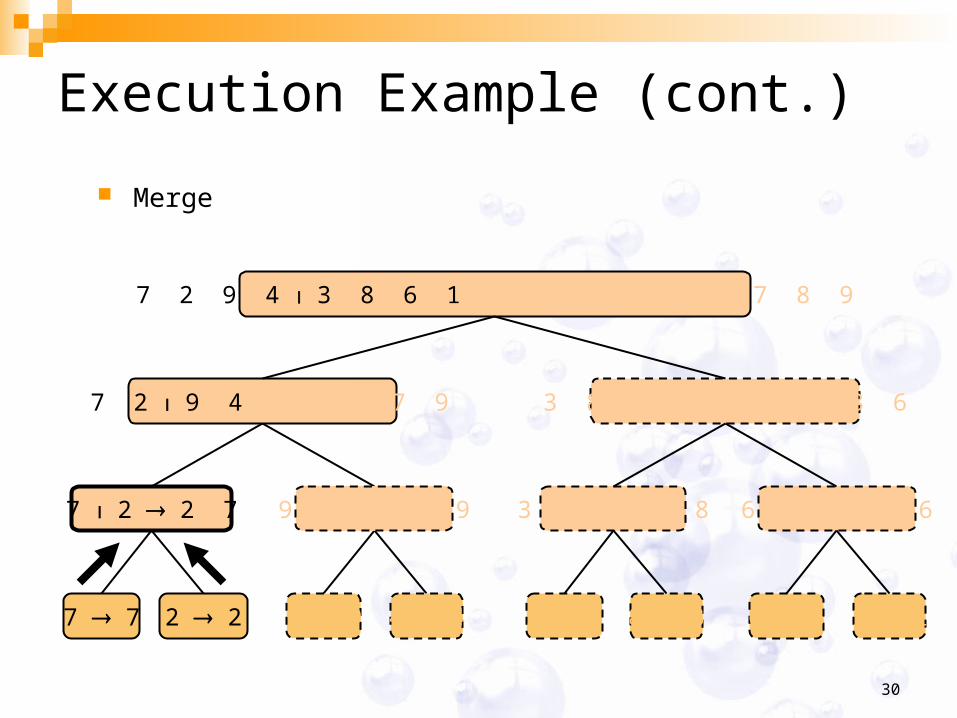
Execution Example (cont.)
Merge
7 2 9 4 2 4 7 9 3 8 6 1 1 3 8 6
7 2 2 7 9 4 4 9 3 8 3 8 6 1 1 6
7 7 2 2 9 9 4 4 3 3 8 8 6 6 1 1
7 2 9 4 3 8 6 1 1 2 3 4 6 7 8 9
31
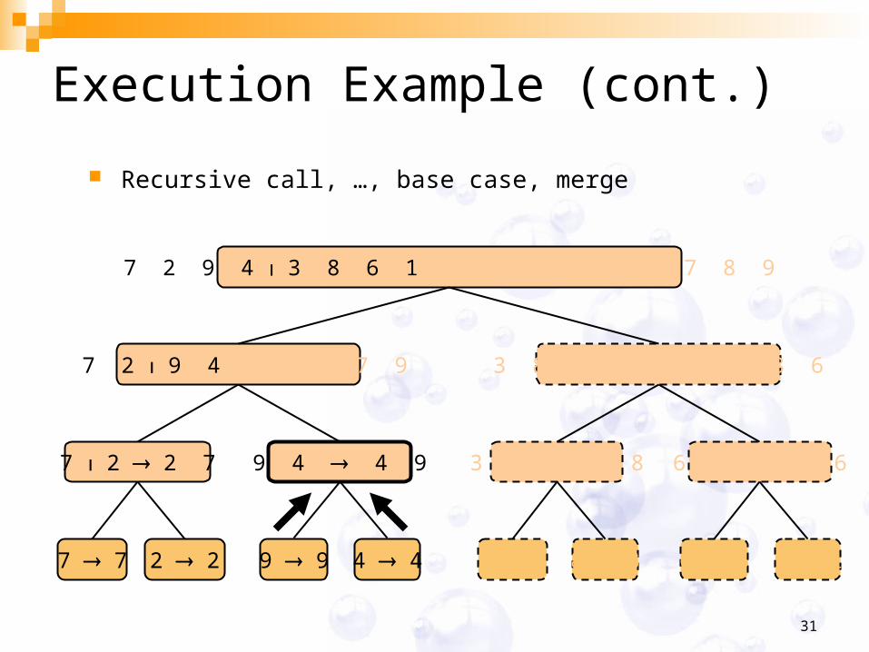
Execution Example (cont.)
Recursive call, …, base case, merge
7 2 9 4 2 4 7 9 3 8 6 1 1 3 8 6
7 2 2 7 9 4 4 9 3 8 3 8 6 1 1 6
7 7 2 2 3 3 8 8 6 6 1 1
7 2 9 4 3 8 6 1 1 2 3 4 6 7 8 9
9 9 4 4
32
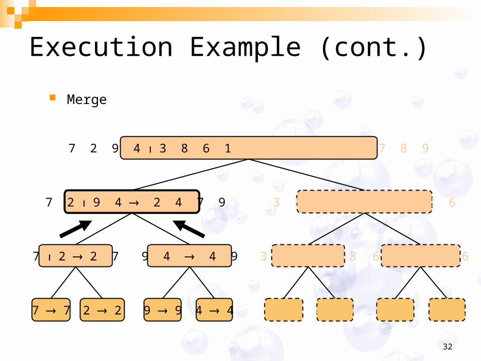
Execution Example (cont.)
Merge
7 2 9 4 2 4 7 9 3 8 6 1 1 3 8 6
7 2 2 7 9 4 4 9 3 8 3 8 6 1 1 6
7 7 2 2 9 9 4 4 3 3 8 8 6 6 1 1
7 2 9 4 3 8 6 1 1 2 3 4 6 7 8 9
33
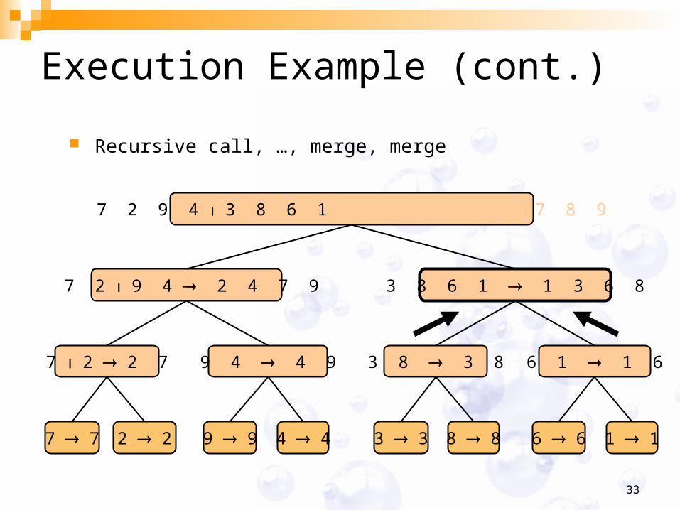
Execution Example (cont.)
Recursive call, …, merge, merge
7 2 9 4 2 4 7 9 3 8 6 1 1 3 6 8
7 2 2 7 9 4 4 9 3 8 3 8 6 1 1 6
7 7 2 2 9 9 4 4 3 3 8 8 6 6 1 1
7 2 9 4 3 8 6 1 1 2 3 4 6 7 8 9
34
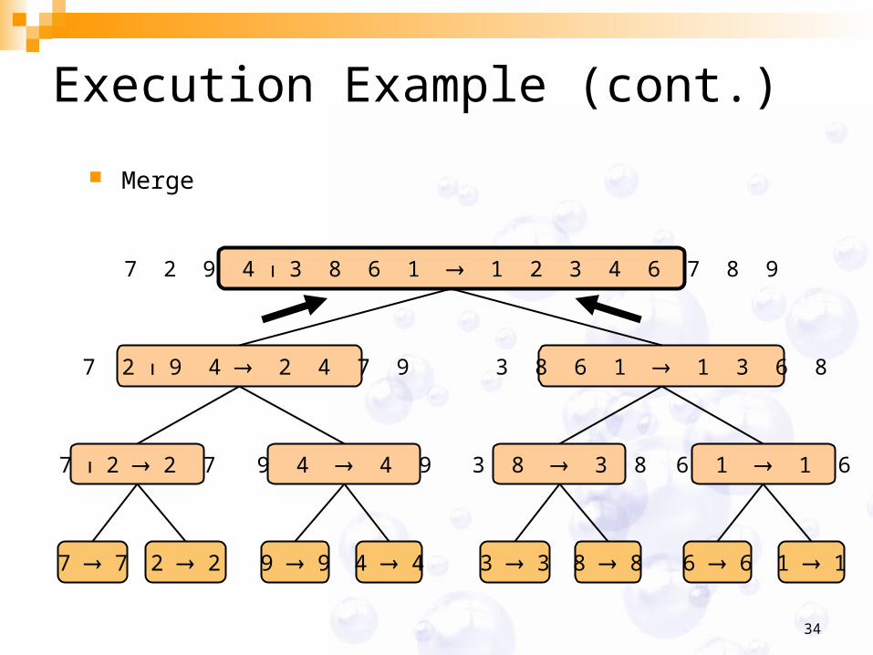
Execution Example (cont.)
Merge
7 2 9 4 2 4 7 9 3 8 6 1 1 3 6 8
7 2 2 7 9 4 4 9 3 8 3 8 6 1 1 6
7 7 2 2 9 9 4 4 3 3 8 8 6 6 1 1
7 2 9 4 3 8 6 1 1 2 3 4 6 7 8 9
35
auxiliary array
smallest smallest
A G L O R H I M S T
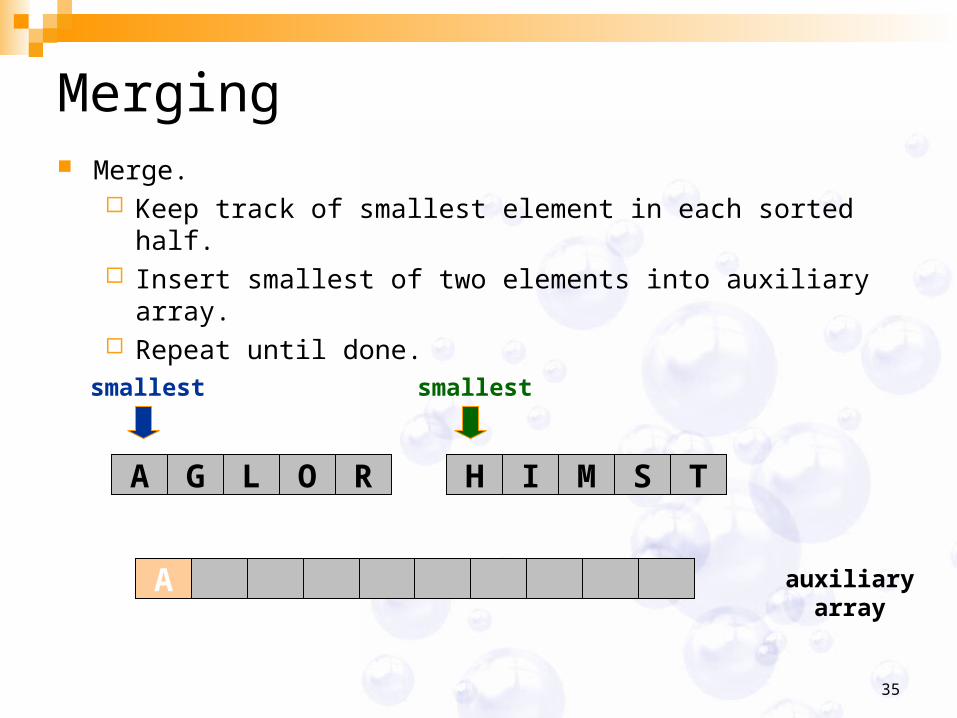
Merging Merge.
Keep track of smallest element in each sorted half. Insert smallest of two elements into auxiliary array. Repeat until done.
A
36
auxiliary array
smallest smallest
A G L O R H I M S T
A
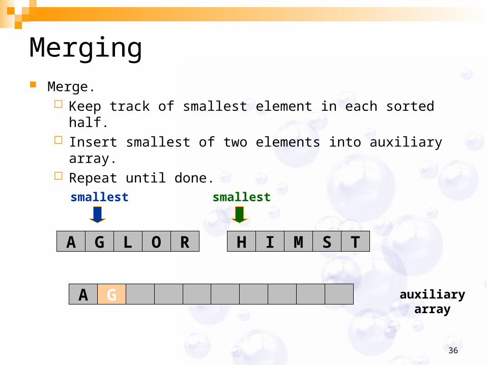
Merging Merge.
Keep track of smallest element in each sorted half. Insert smallest of two elements into auxiliary array. Repeat until done.
G
37
auxiliary array
smallest smallest
A G L O R H I M S T
A G
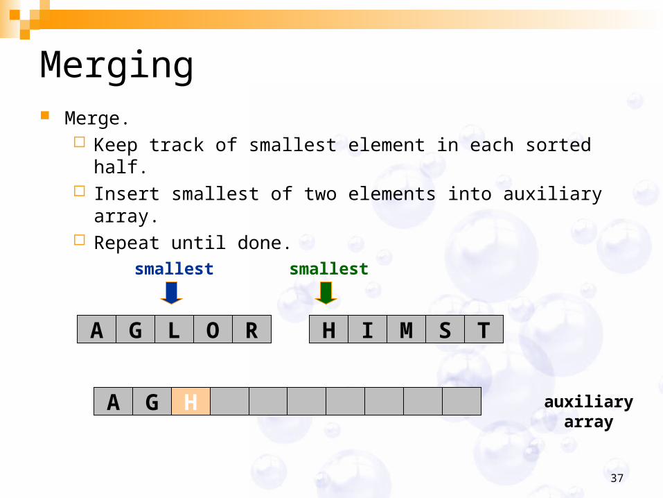
Merging Merge.
Keep track of smallest element in each sorted half. Insert smallest of two elements into auxiliary array. Repeat until done.
H
38
auxiliary array
smallest smallest
A G L O R H I M S T
A G H
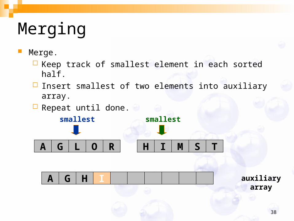
Merging Merge.
Keep track of smallest element in each sorted half. Insert smallest of two elements into auxiliary array. Repeat until done.
I

39
auxiliary array
smallest smallest
A G L O R H I M S T
A G H I
Merging Merge.
Keep track of smallest element in each sorted half. Insert smallest of two elements into auxiliary array. Repeat until done.
L
40
auxiliary array
smallest smallest
A G L O R H I M S T
A G H I L
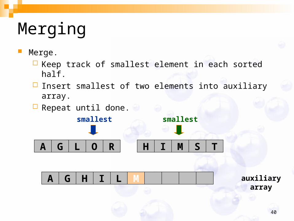
Merging Merge.
Keep track of smallest element in each sorted half. Insert smallest of two elements into auxiliary array. Repeat until done.
M
41
auxiliary array
smallest smallest
A G L O R H I M S T
A G H I L M
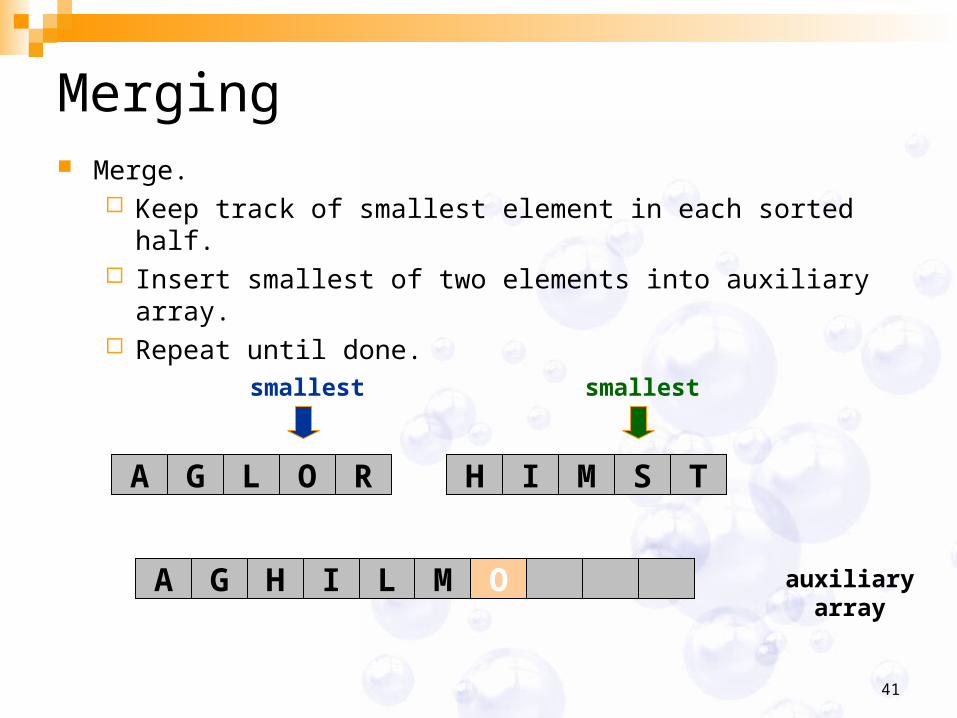
Merging Merge.
Keep track of smallest element in each sorted half. Insert smallest of two elements into auxiliary array. Repeat until done.
O
42
auxiliary array
smallest smallest
A G L O R H I M S T
A G H I L M O
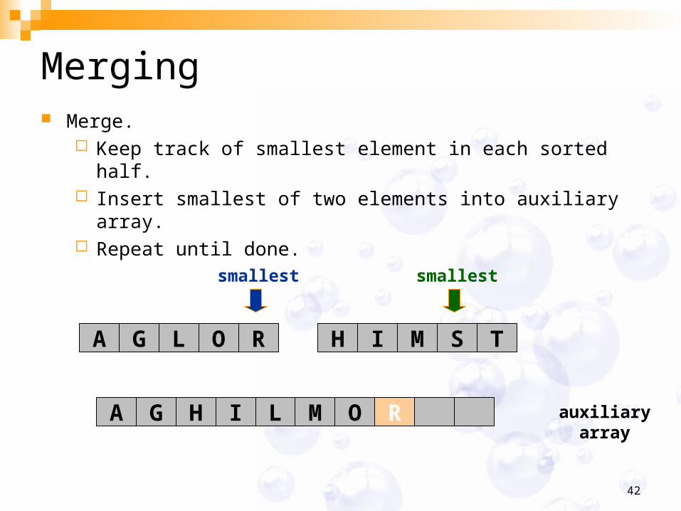
Merging Merge.
Keep track of smallest element in each sorted half. Insert smallest of two elements into auxiliary array. Repeat until done.
R
43
auxiliary array
first halfexhausted smallest
A G L O R H I M S T
A G H I L M O R
Merging Merge.
Keep track of smallest element in each sorted half. Insert smallest of two elements into auxiliary array. Repeat until done.
S
44
auxiliary array
first halfexhausted smallest
A G L O R H I M S T
A G H I L M O R S
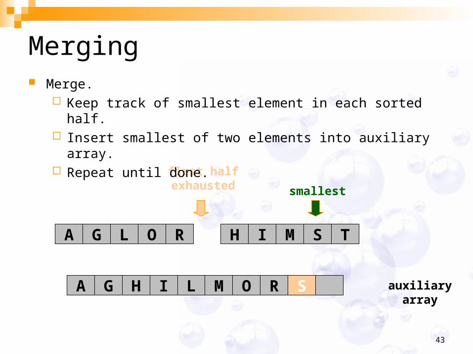
Merging Merge.
Keep track of smallest element in each sorted half. Insert smallest of two elements into auxiliary array. Repeat until done.
T
45
auxiliary array
first halfexhausted
second halfexhausted
A G L O R H I M S T
A G H I L M O R S T
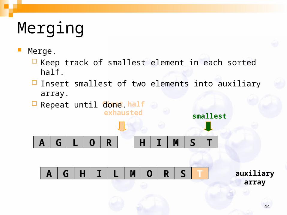
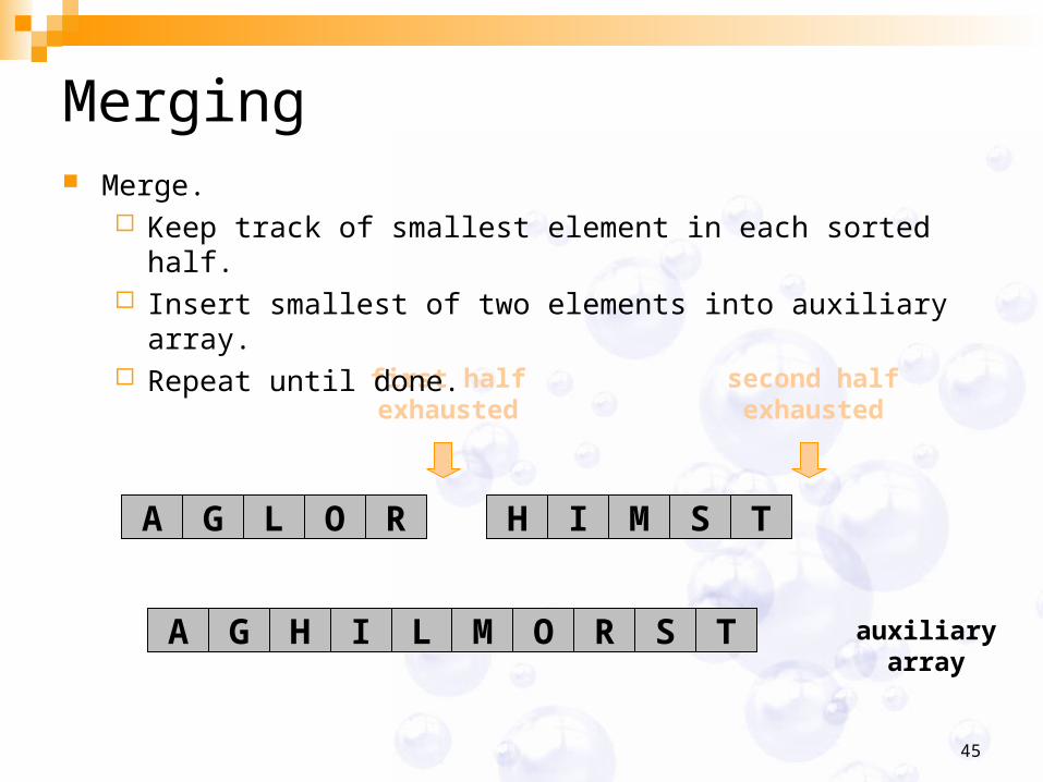
Merging Merge.
Keep track of smallest element in each sorted half. Insert smallest of two elements into auxiliary array. Repeat until done.
46
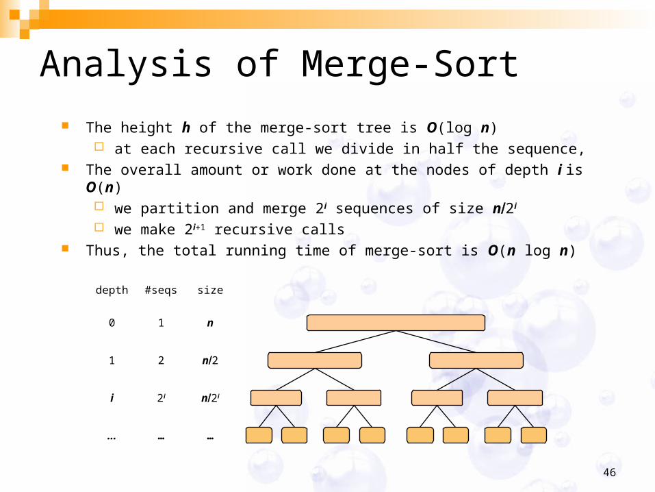
Analysis of Merge-Sort
The height h of the merge-sort tree is O(log n) at each recursive call we divide in half the sequence,
The overall amount or work done at the nodes of depth i is O(n) we partition and merge 2i sequences of size n2i we make 2i1 recursive calls
Thus, the total running time of merge-sort is O(n log n)
depth #seqs size
0 1 n
1 2 n2
i 2i n2i
… … …
47
Merge Sortthe analysis
• MergeSort is a classic example of the techniques used to analyze MergeSort is a classic example of the techniques used to analyze recursive routines:recursive routines:
• Merge Sort is a divide-and-conquer recursive algorithm.Merge Sort is a divide-and-conquer recursive algorithm.
• MergeSort’s running time time is MergeSort’s running time time is O(N log N).O(N log N).
48
Merge Sortthe analysis
• Although its running time is O(N log N), it is hardly ever used for the main Although its running time is O(N log N), it is hardly ever used for the main memory sorts that’s because it consumes a lot of memory.memory sorts that’s because it consumes a lot of memory.
• The The main problemmain problem is that merging two sorted lists requires is that merging two sorted lists requires linear extra linear extra memorymemory, and the additional work spent copying to the temporary array and , and the additional work spent copying to the temporary array and back throughout the algorithm.back throughout the algorithm.
• Which effect in Which effect in slowing down the sortslowing down the sort..
The principal shortcoming of mergesort is the linear amount of extra storage the algorithm requires.
Though merging can be done in place, the resulting algorithm is quite complicated and, since it has a significantly larger multiplicative constant, the in-place mergesort is of theoretical interest only.
49
Divide & Conquer: Quicksort
Lecture 05.2
Asst. Prof. Dr. Bunyarit UyyanonvaraAsst. Prof. Dr. Bunyarit UyyanonvaraIT Program, Image and Vision Computing Lab.
School of Information and Computer Technology
Sirindhorn International Institute of Technology
Thammasat Universityhttp://www.siit.tu.ac.th/bunyarit
[email protected] 5013505 X 2005
ITS033 – Programming & Algorithms
50
Quick Sortthe algorithm
• Quick SortQuick Sort's approach is to take 's approach is to take Merge Sort'sMerge Sort's philosophy philosophy but but eliminateeliminate the need for the merging steps. the need for the merging steps.
• Can you see how the problem could be solved ?Can you see how the problem could be solved ?

51
Quick Sortthe algorithm
• It makes sure that every data item in the first sub-list It makes sure that every data item in the first sub-list is less than every data item in the second sub-list.is less than every data item in the second sub-list.
• The procedure that accomplished that is called The procedure that accomplished that is called ""partitioningpartitioning" the data. After the paritioning,,each of the " the data. After the paritioning,,each of the sub-lists are sorted, which will cause the entire array to sub-lists are sorted, which will cause the entire array to be sorted.be sorted.
52
Quick-Sort
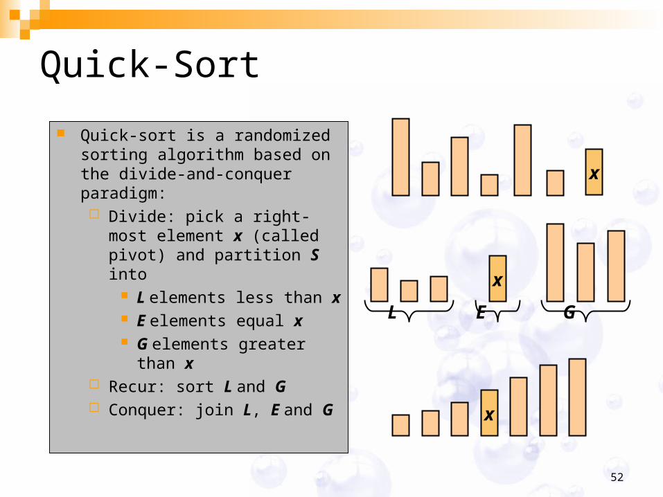
Quick-sort is a randomized sorting algorithm based on the divide-and-conquer paradigm: Divide: pick a right-most
element x (called pivot) and partition S into
L elements less than x E elements equal x G elements greater
than x Recur: sort L and G Conquer: join L, E and G
x
x
L GE
x
53
Quick Sort
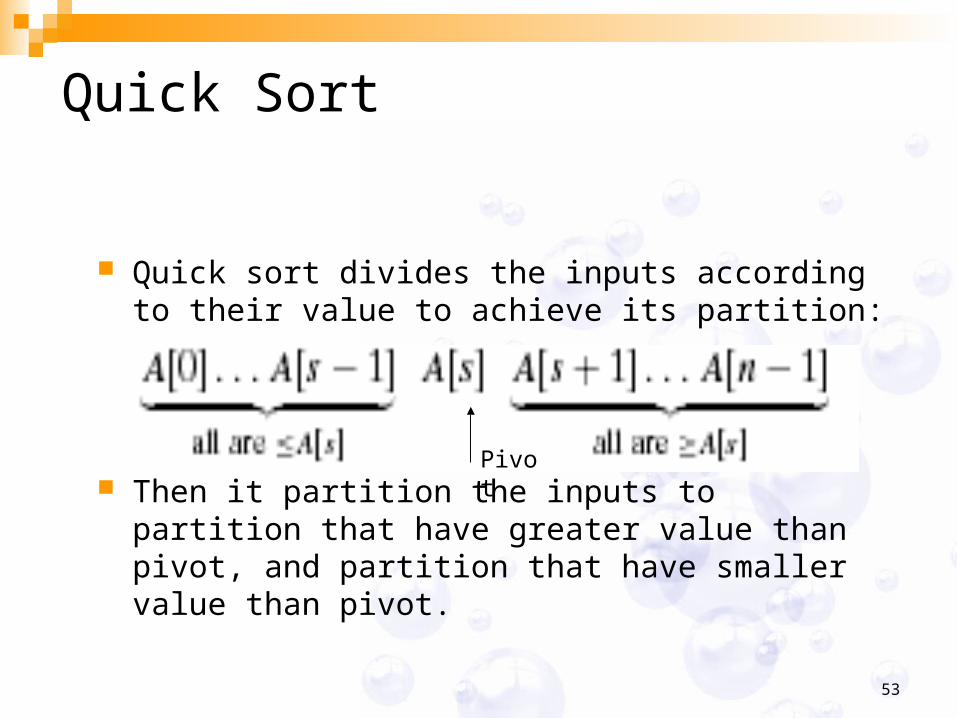
Quick sort divides the inputs according to their value to achieve its partition:
Then it partition the inputs to partition that have greater value than pivot, and partition that have smaller value than pivot.
Pivot
54
Quick Sort
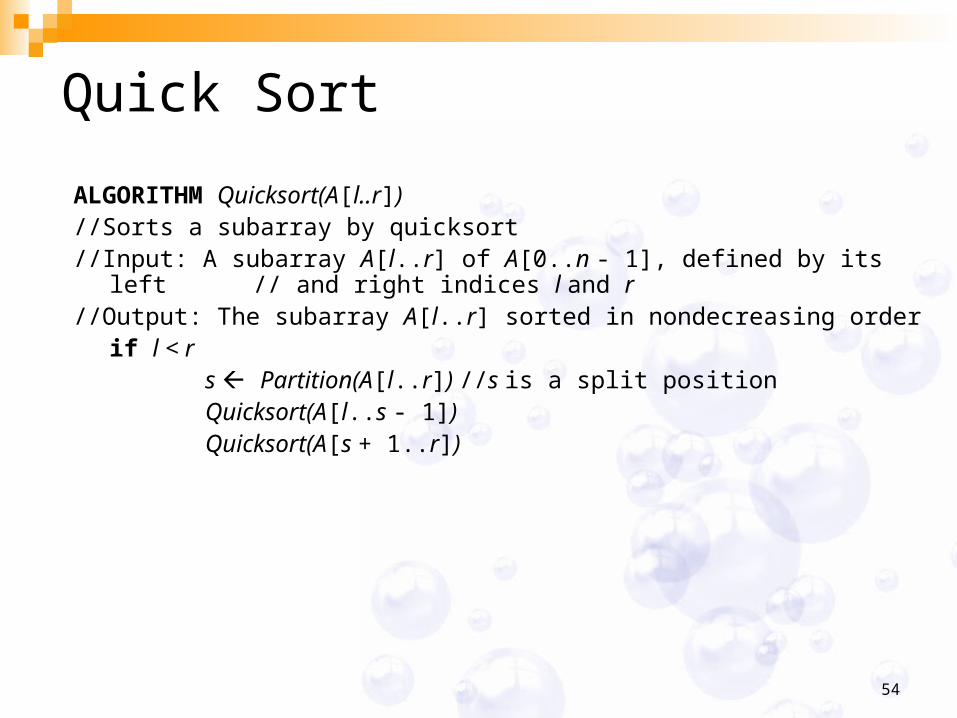
ALGORITHM Quicksort(A[l..r])//Sorts a subarray by quicksort//Input: A subarray A[l..r] of A[0..n - 1], defined by its left // and
right indices l and r//Output: The subarray A[l..r] sorted in nondecreasing order
if l < rs Partition(A[l..r]) //s is a split positionQuicksort(A[l..s - 1])Quicksort(A[s + 1..r])
55
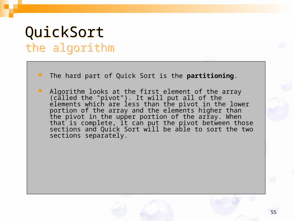
The hard part of Quick Sort is the The hard part of Quick Sort is the partitioningpartitioning. .
Algorithm looks at the first element of the array (called the "pivot"). It Algorithm looks at the first element of the array (called the "pivot"). It will put all of the elements which are less than the pivot in the lower will put all of the elements which are less than the pivot in the lower portion of the array and the elements higher than the pivot in the upper portion of the array and the elements higher than the pivot in the upper portion of the array. When that is complete, it can put the pivot portion of the array. When that is complete, it can put the pivot between those sections and Quick Sort will be able to sort the two between those sections and Quick Sort will be able to sort the two sections separately. sections separately.
QuickSortthe algorithmQuickSortthe algorithm
56
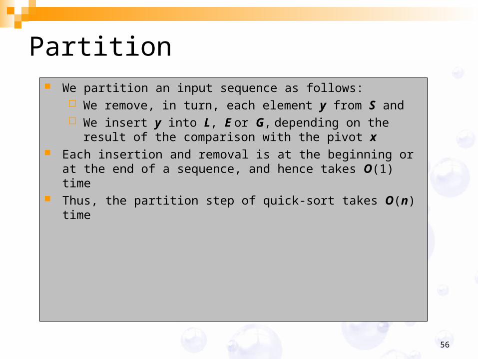
Partition We partition an input sequence as follows:
We remove, in turn, each element y from S and We insert y into L, E or G, depending on the result of
the comparison with the pivot x Each insertion and removal is at the beginning or at the
end of a sequence, and hence takes O(1) time Thus, the partition step of quick-sort takes O(n) time
57
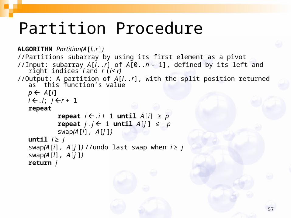
Partition ProcedureALGORITHM Partition(A[l..r])//Partitions subarray by using its first element as a pivot//Input: subarray A[l..r] of A[0..n - 1], defined by its left and right indices l and
r (l< r)//Output: A partition of A[l..r], with the split position returned as this
function’s valuep A[l]i .l; j r + 1repeat
repeat i .i + 1 until A[i] ≥ prepeat j .j 1 until A[j ] ≤ pswap(A[i], A[j ])
until i ≥ jswap(A[i], A[j ]) //undo last swap when i ≥ jswap(A[l], A[j ])return j
58
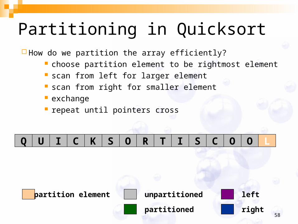
Partitioning in Quicksort How do we partition the array efficiently?
choose partition element to be rightmost element scan from left for larger element scan from right for smaller element exchange repeat until pointers cross
Q U I C K S O R T I S C O O L
partitioned
partition element left
right
unpartitioned

59
Partitioning in Quicksort How do we partition the array efficiently?
choose partition element to be rightmost element scan from left for larger element scan from right for smaller element exchange repeat until pointers crossswap me
partitioned
partition element left
right
unpartitioned
Q U I C K S O R T I S C O O L

60
Partitioning in Quicksort How do we partition the array efficiently?
choose partition element to be rightmost element scan from left for larger element scan from right for smaller element exchange repeat until pointers cross
partitioned
partition element left
right
unpartitioned
swap me
Q U I C K S O R T I S C O O L

61
Partitioning in Quicksort How do we partition the array efficiently?
choose partition element to be rightmost element scan from left for larger element scan from right for smaller element exchange repeat until pointers cross
partitioned
partition element left
right
unpartitioned
swap me
Q U I C K S O R T I S C O O L
62
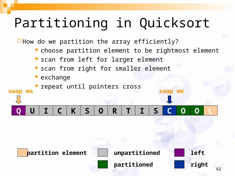
Partitioning in Quicksort How do we partition the array efficiently?
choose partition element to be rightmost element scan from left for larger element scan from right for smaller element exchange repeat until pointers cross
partitioned
partition element left
right
unpartitioned
swap me
Q U I C K S O R T I S C O O L
swap me
63
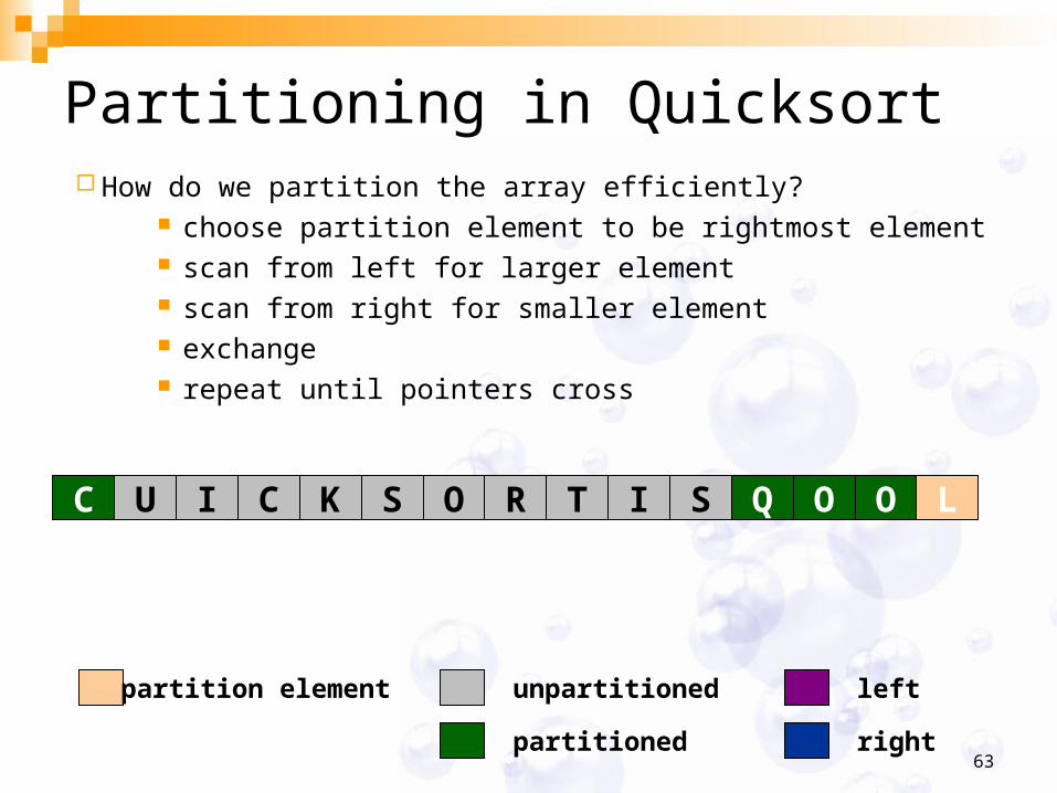
Partitioning in Quicksort How do we partition the array efficiently?
choose partition element to be rightmost element scan from left for larger element scan from right for smaller element exchange repeat until pointers cross
partitioned
partition element left
right
unpartitioned
C U I C K S O R T I S Q O O L
64
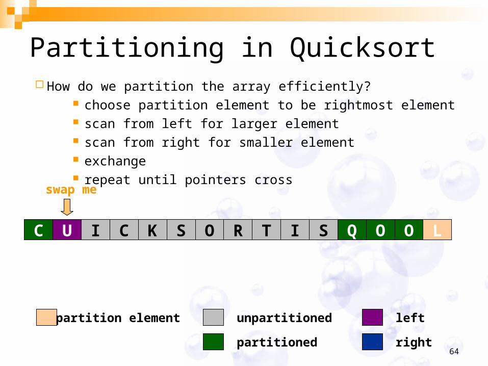
Partitioning in Quicksort How do we partition the array efficiently?
choose partition element to be rightmost element scan from left for larger element scan from right for smaller element exchange repeat until pointers crossswap me
partitioned
partition element left
right
unpartitioned
C U I C K S O R T I S Q O O L
65
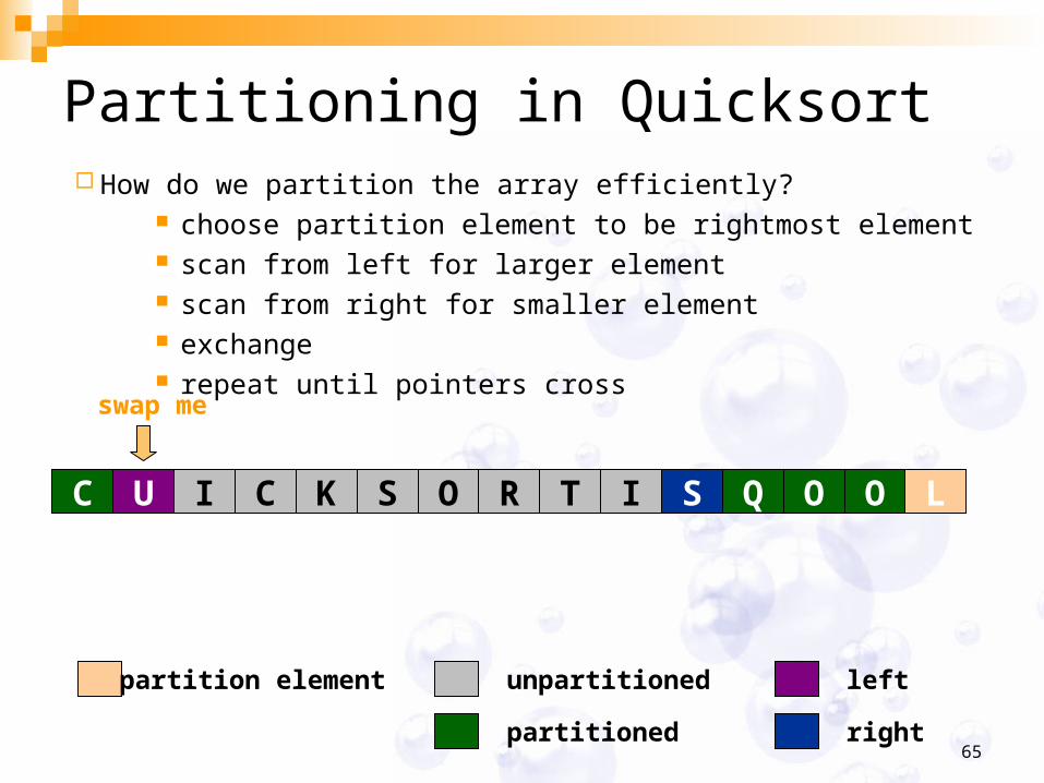
Partitioning in Quicksort How do we partition the array efficiently?
choose partition element to be rightmost element scan from left for larger element scan from right for smaller element exchange repeat until pointers cross
partitioned
partition element left
right
unpartitioned
swap me
C U I C K S O R T I S Q O O L
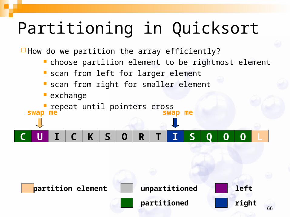
66
Partitioning in Quicksort How do we partition the array efficiently?
choose partition element to be rightmost element scan from left for larger element scan from right for smaller element exchange repeat until pointers cross
partitioned
partition element left
right
unpartitioned
swap me
C U I C K S O R T I S Q O O L
swap me
67
Partitioning in Quicksort How do we partition the array efficiently?
choose partition element to be rightmost element scan from left for larger element scan from right for smaller element exchange repeat until pointers cross
partitioned
partition element left
right
unpartitioned
C I I C K S O R T U S Q O O L
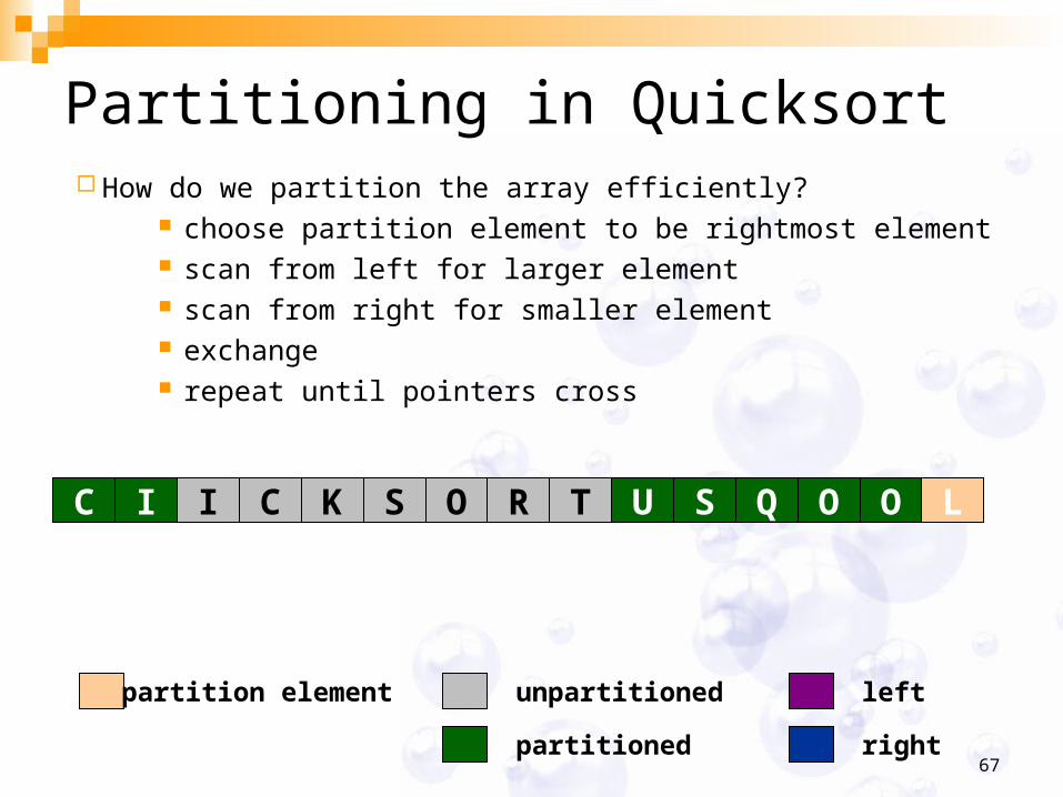
68
Partitioning in Quicksort How do we partition the array efficiently?
choose partition element to be rightmost element scan from left for larger element scan from right for smaller element exchange repeat until pointers cross
partitioned
partition element left
right
unpartitioned
C I I C K S O R T U S Q O O L
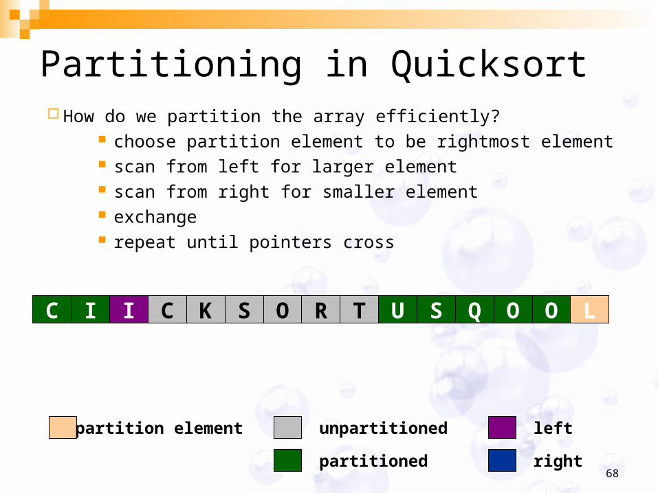
69
Partitioning in Quicksort How do we partition the array efficiently?
choose partition element to be rightmost element scan from left for larger element scan from right for smaller element exchange repeat until pointers cross
partitioned
partition element left
right
unpartitioned
C I I C K S O R T U S Q O O L
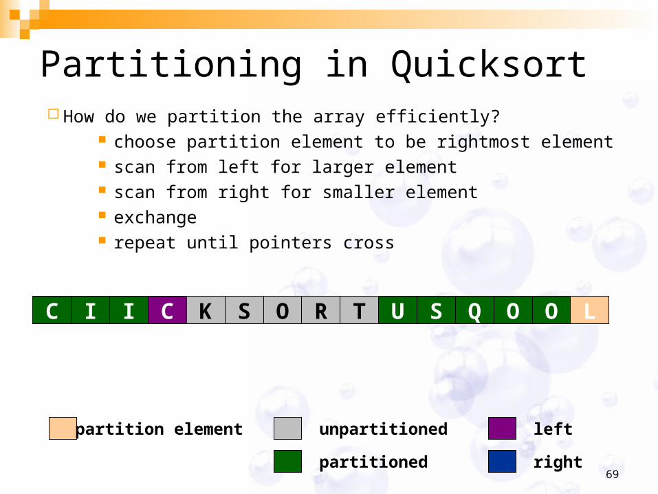
70
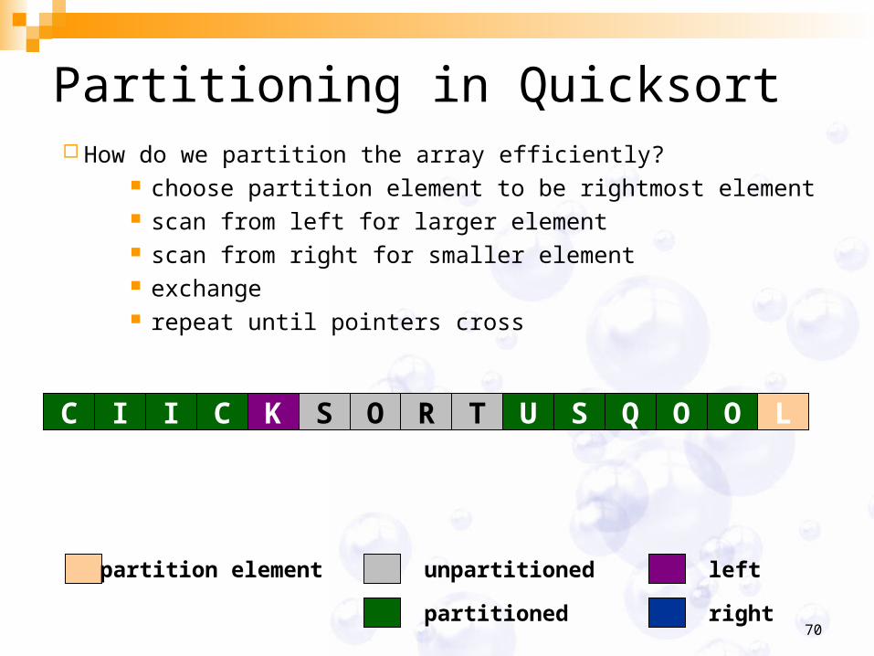
Partitioning in Quicksort How do we partition the array efficiently?
choose partition element to be rightmost element scan from left for larger element scan from right for smaller element exchange repeat until pointers cross
partitioned
partition element left
right
unpartitioned
C I I C K S O R T U S Q O O L
71
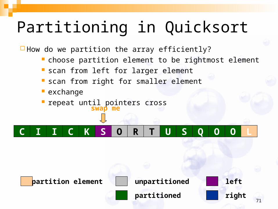
Partitioning in Quicksort How do we partition the array efficiently?
choose partition element to be rightmost element scan from left for larger element scan from right for smaller element exchange repeat until pointers crossswap me
partitioned
partition element left
right
unpartitioned
C I I C K S O R T U S Q O O L
72
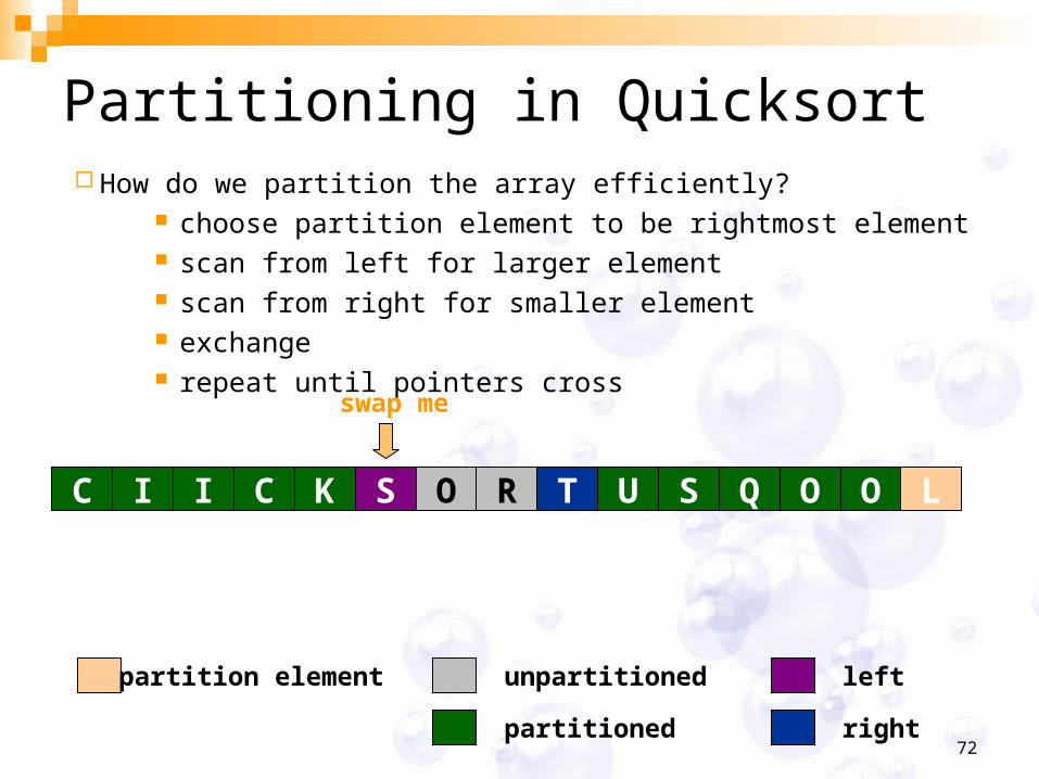
Partitioning in Quicksort How do we partition the array efficiently?
choose partition element to be rightmost element scan from left for larger element scan from right for smaller element exchange repeat until pointers cross
partitioned
partition element left
right
unpartitioned
swap me
C I I C K S O R T U S Q O O L
73
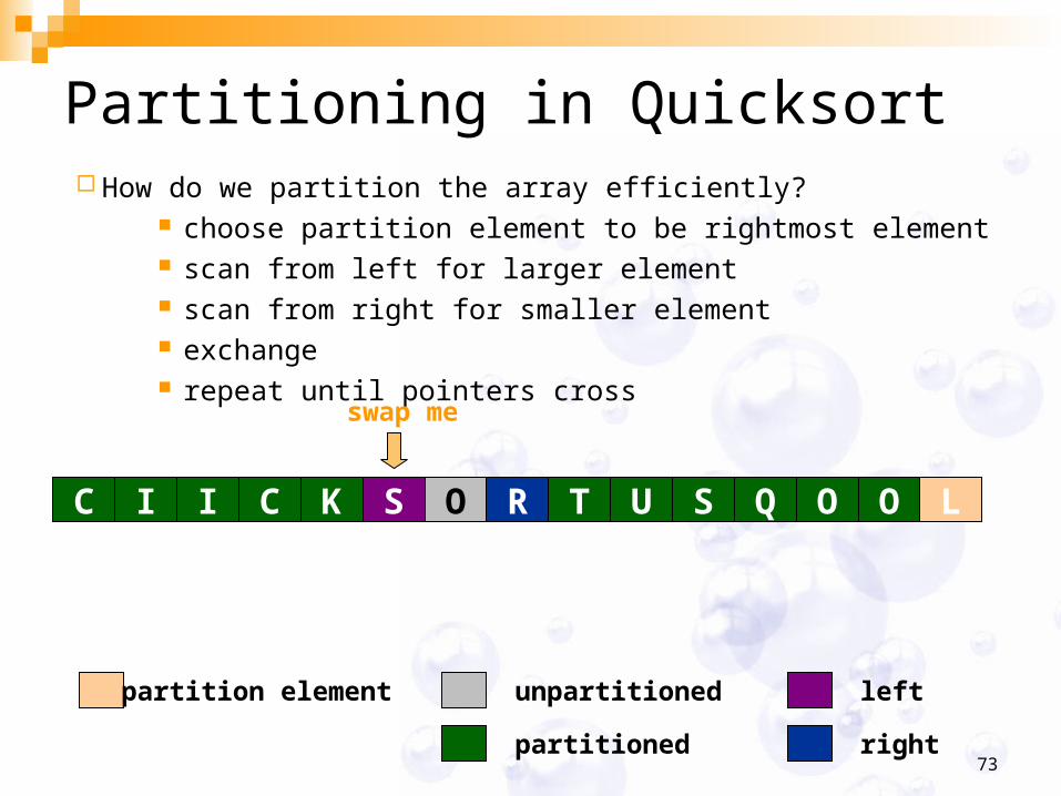
Partitioning in Quicksort How do we partition the array efficiently?
choose partition element to be rightmost element scan from left for larger element scan from right for smaller element exchange repeat until pointers cross
partitioned
partition element left
right
unpartitioned
swap me
C I I C K S O R T U S Q O O L

74
Partitioning in Quicksort How do we partition the array efficiently?
choose partition element to be rightmost element scan from left for larger element scan from right for smaller element exchange repeat until pointers cross
partitioned
partition element left
right
unpartitioned
swap me
C I I C K S O R T U S Q O O L

75
Partitioning in Quicksort How do we partition the array efficiently?
choose partition element to be rightmost element scan from left for larger element scan from right for smaller element exchange repeat until pointers crosspointers cross
swap with partitioning element
partitioned
partition element left
right
unpartitioned
C I I C K S O R T U S Q O O L
76
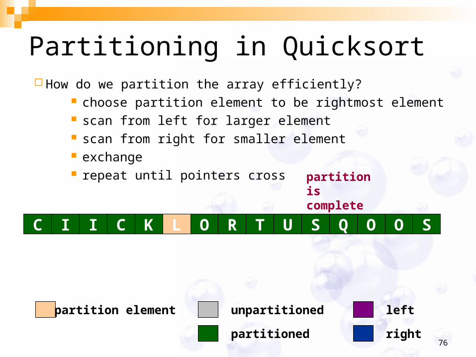
Partitioning in Quicksort How do we partition the array efficiently?
choose partition element to be rightmost element scan from left for larger element scan from right for smaller element exchange repeat until pointers cross
partitioned
partition element left
right
unpartitioned
partition is complete
C I I C K L O R T U S Q O O S
77
Quick Sortthe analysis
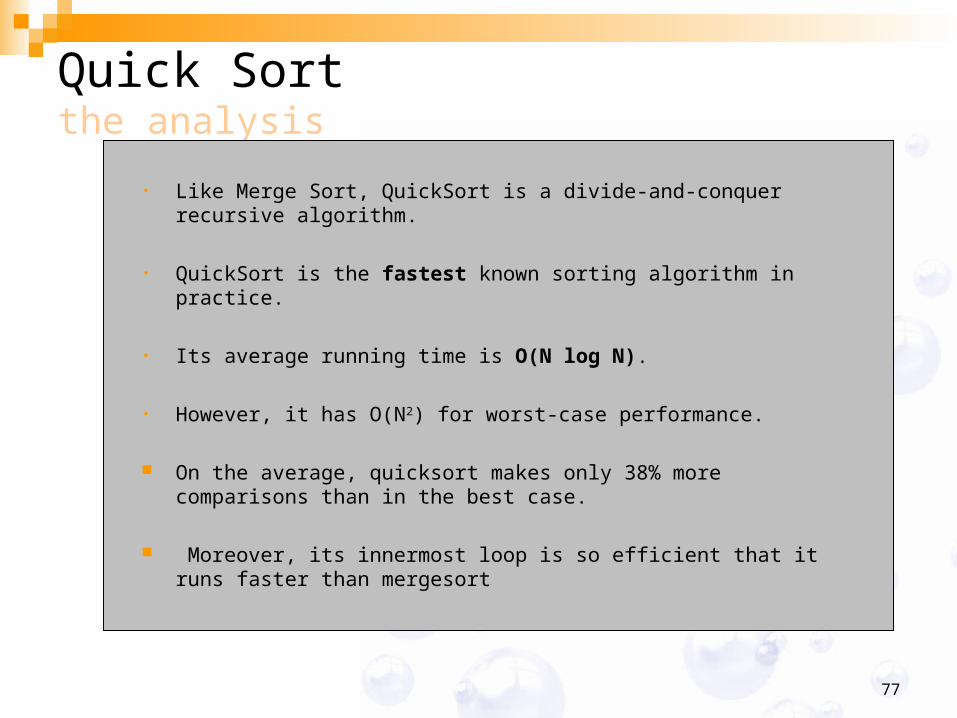
• Like Merge Sort, QuickSort is a divide-and-conquer recursive algorithm.Like Merge Sort, QuickSort is a divide-and-conquer recursive algorithm.
• QuickSort is the QuickSort is the fastest fastest known sorting algorithm in practice.known sorting algorithm in practice.
• Its average running time is Its average running time is O(N log N)O(N log N)..
• However, it has O(NHowever, it has O(N22) for worst-case performance.) for worst-case performance.
On the average, quicksort makes only 38% more comparisons than in the best case.
Moreover, its innermost loop is so efficient that it runs faster than mergesort
78
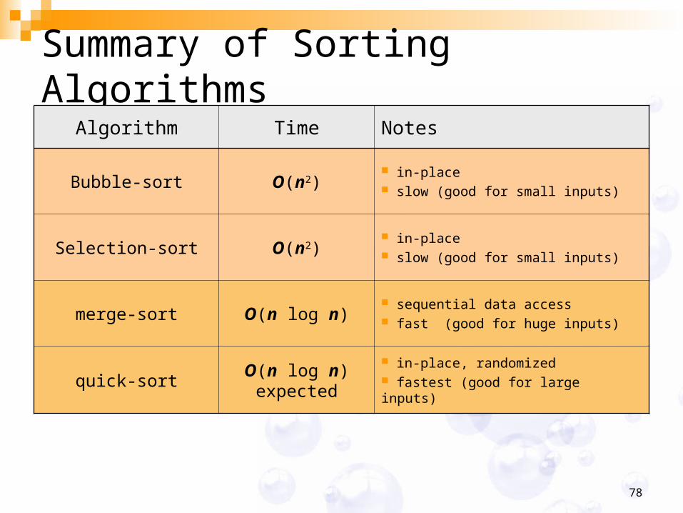
Summary of Sorting Algorithms
Algorithm Time Notes
Bubble-sort O(n2) in-place slow (good for small inputs)
Selection-sort O(n2) in-place slow (good for small inputs)
merge-sort O(n log n) sequential data access fast (good for huge inputs)
quick-sortO(n log n)expected
in-place, randomized fastest (good for large inputs)

79
Divide & Conquer: Binary Search
Lecture 05.3
Asst. Prof. Dr. Bunyarit UyyanonvaraAsst. Prof. Dr. Bunyarit UyyanonvaraIT Program, Image and Vision Computing Lab.
School of Information and Computer Technology
Sirindhorn International Institute of Technology
Thammasat Universityhttp://www.siit.tu.ac.th/bunyarit
[email protected] 5013505 X 2005
ITS033 – Programming & Algorithms
80
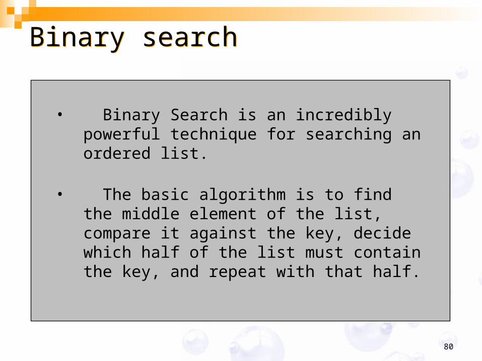
• Binary Search is an incredibly powerful Binary Search is an incredibly powerful technique for searching an ordered list. technique for searching an ordered list.
• The basic algorithm is to find the middle The basic algorithm is to find the middle element of the list, compare it against the element of the list, compare it against the key, decide which half of the list must key, decide which half of the list must contain the key, and repeat with that half. contain the key, and repeat with that half.
Binary searchBinary search

81
Binary Search
It works by comparing a search key K with the array’s middle element A[m].
If they match, the algorithm stops; otherwise, the same operation is repeated recursively for the first half of the array ifK <A[m] and for the second half ifK >A[m]:

82
Binary searchBinary search
Algorithm Algorithm BinarySearchOnSortedBinarySearchOnSortedInput: an array, a keyInput: an array, a keyOutput: Location of the keyOutput: Location of the key
1.1. Sort the array (smallest to biggest)Sort the array (smallest to biggest)2.2. start with the middle element of the array start with the middle element of the array
If it matches then doneIf it matches then doneIf middle element > key then search array’s 1st If middle element > key then search array’s 1st
halfhalfIf middle element < key then search array’s 2nd If middle element < key then search array’s 2nd
halfhalf
83
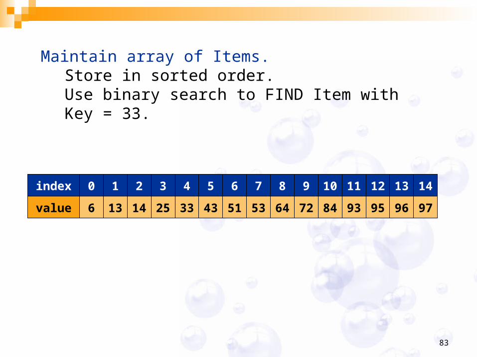
821 3 4 65 7index 109 11 12 14130
641413 25 33 5143 53value 8472 93 95 97966
Maintain array of Items.Store in sorted order.Use binary search to FIND Item with Key = 33.
84
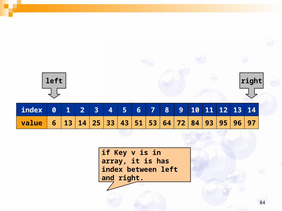
821 3 4 65 7index 109 11 12 14130
641413 25 33 5143 53value 8472 93 95 97966
rightleft
if Key v is in array, it is has index between left and right.
85
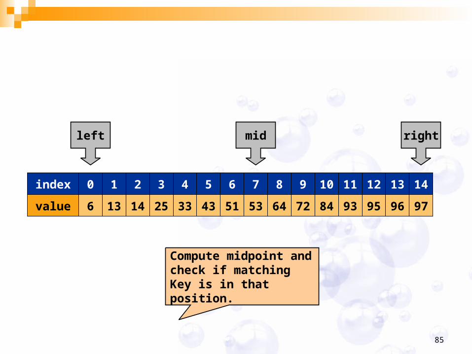
821 3 4 65 7index 109 11 12 14130
641413 25 33 5143 53value 8472 93 95 97966
rightleft mid
Compute midpoint and check if matching Key is in that position.
86
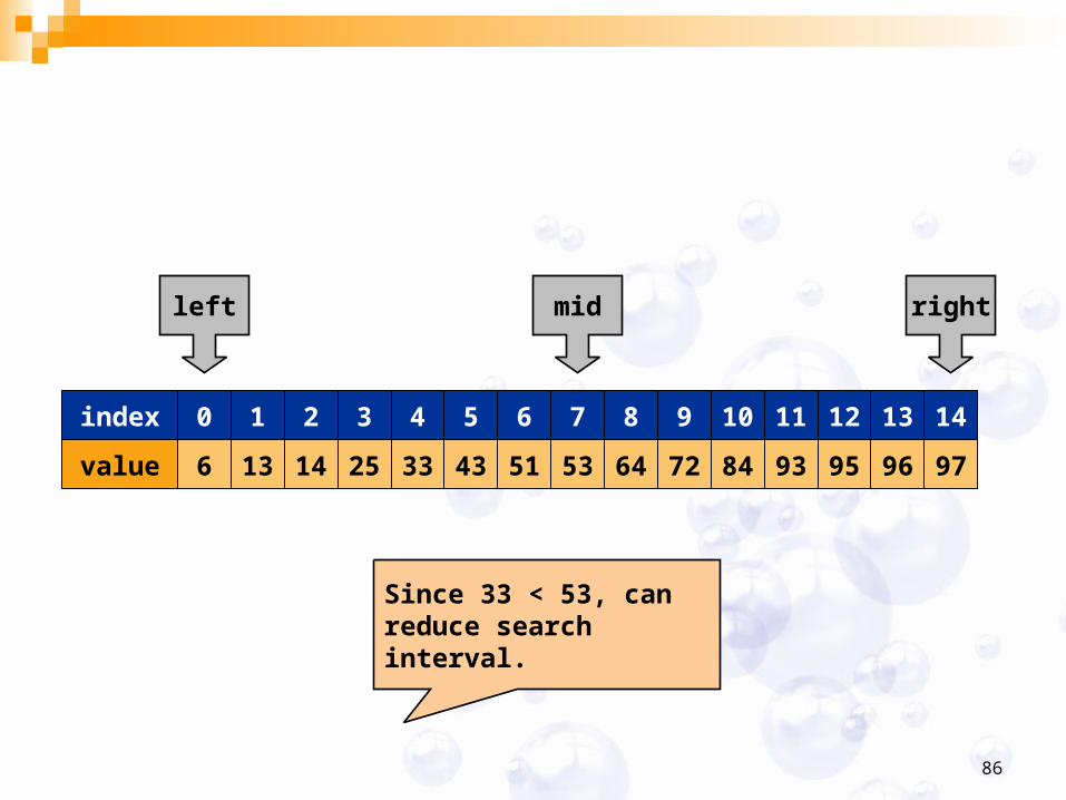
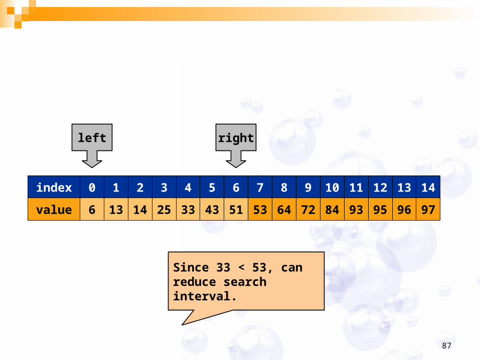
821 3 4 65 7index 109 11 12 14130
641413 25 33 5143 53value 8472 93 95 97966
rightleft mid
Since 33 < 53, can reduce search interval.
87
821 3 4 65 7index 109 11 12 14130
641413 25 33 5143 53value 8472 93 95 97966
rightleft
Since 33 < 53, can reduce search interval.
88
821 3 4 65 7index 109 11 12 14130
641413 25 33 5143 53value 8472 93 95 97966
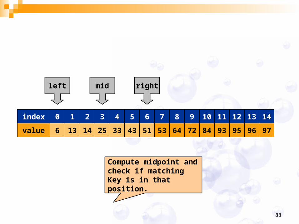
rightleft mid
Compute midpoint and check if matching Key is in that position.
89
821 3 4 65 7index 109 11 12 14130
641413 25 33 5143 53value 8472 93 95 97966
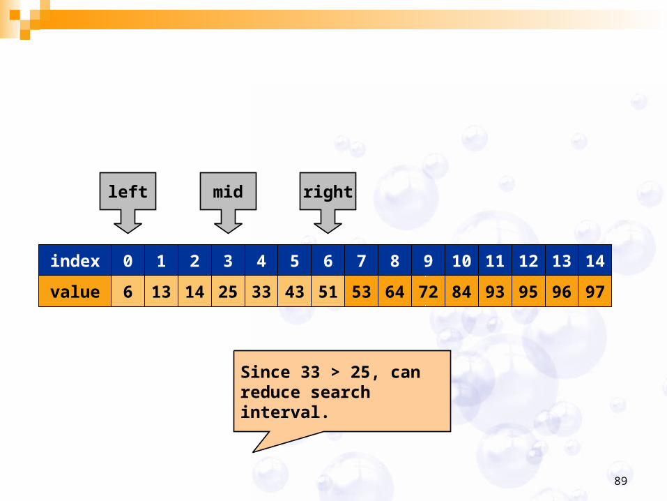
rightleft mid
Since 33 > 25, can reduce search interval.
90
821 3 4 65 7index 109 11 12 14130
641413 25 33 5143 53value 8472 93 95 97966
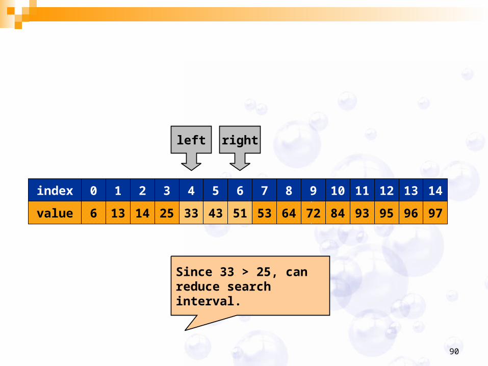
rightleft
Since 33 > 25, can reduce search interval.
91
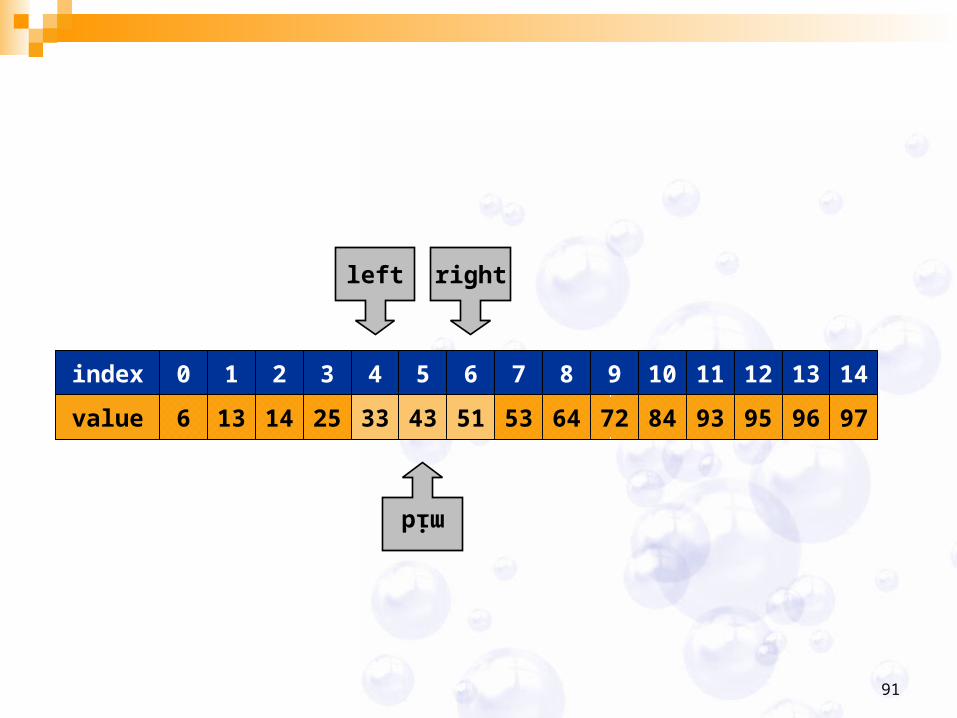
821 3 4 65 7index 109 11 12 14130
641413 25 33 5143 53value 8472 93 95 97966
rightleft
mid
92
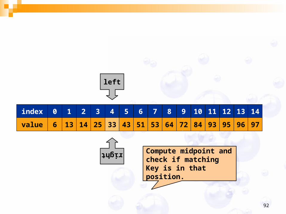
821 3 4 65 7index 109 11 12 14130
641413 25 33 5143 53value 8472 93 95 97966
left
right
Compute midpoint and check if matching Key is in that position.
93
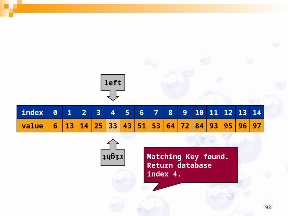
821 3 4 65 7index 109 11 12 14130
641413 25 33 5143 53value 8472 93 95 97966
left
right
Matching Key found. Return database index 4.
94
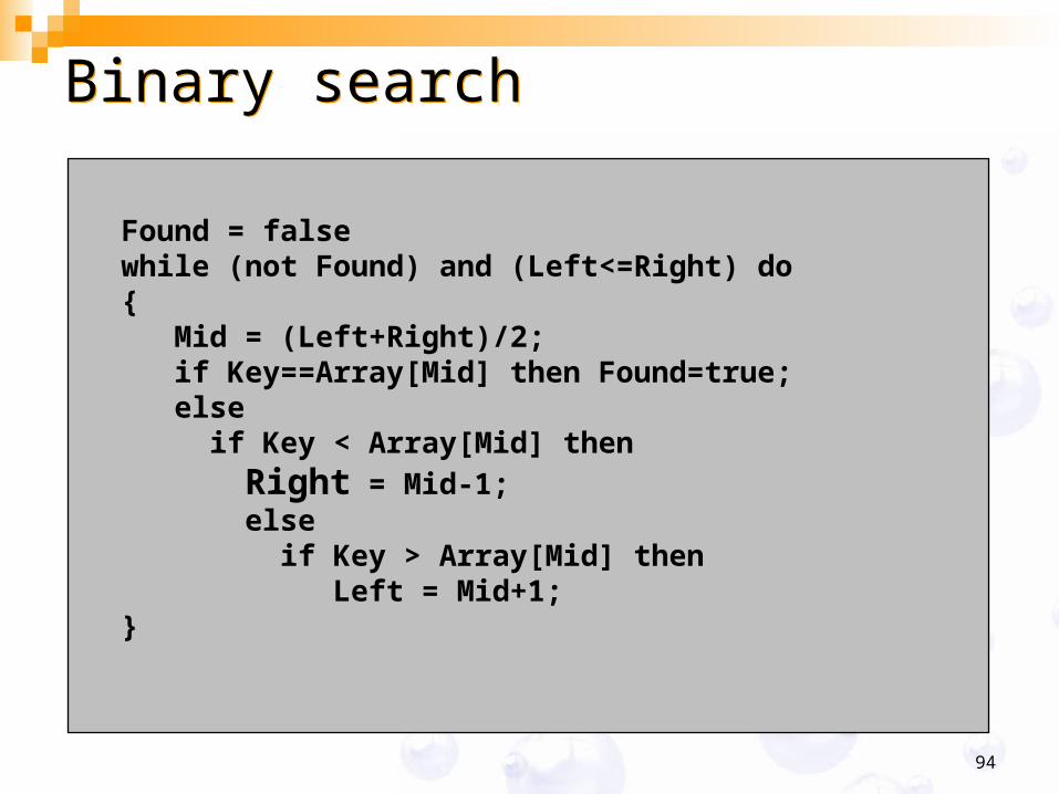
Binary searchBinary search
Found = falsewhile (not Found) and (Left<=Right) do{ Mid = (Left+Right)/2; if Key==Array[Mid] then Found=true; else if Key < Array[Mid] then Right = Mid-1; else if Key > Array[Mid] then Left = Mid+1;}
95
Binary searchBinary search
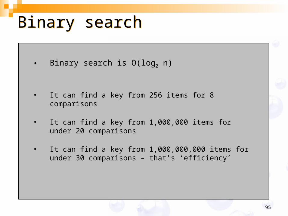
• Binary search is O(log2 n)
• It can find a key from 256 items for 8 comparisons
• It can find a key from 1,000,000 items for under 20 comparisons
• It can find a key from 1,000,000,000 items for under 30 comparisons – that’s ‘efficiency’

96
Divide & Conquer: Closest Pair Problem
Lecture 05.4
Asst. Prof. Dr. Bunyarit UyyanonvaraAsst. Prof. Dr. Bunyarit UyyanonvaraIT Program, Image and Vision Computing Lab.
School of Information and Computer Technology
Sirindhorn International Institute of Technology
Thammasat Universityhttp://www.siit.tu.ac.th/bunyarit
[email protected] 5013505 X 2005
ITS033 – Programming & Algorithms
97
Closest-Pair Problems by Divide-and-ConquerClosest-Pair Problem Let P1 = (x1, y1), . . . , Pn = (xn, yn) be a set S of n points in the
plane, where n, for simplicity, is a power of two. We can divide the points given into two subsets S1 and S2 of n/2 points each by drawing a vertical line x = c.
Thus, n/2 points lie to the left of or on the line itself and n/2 points lie to the right of or on the line.
98
Closest-Pair Problem Following the divide-and-conquer approach, we can find
recursively the closest pairs for the left subset S1 and the right subset S2. Let d1 and d2 be the smallest distances between pairs of points in S1 and S2, respectively, and let d = min{d1, d2}.
Unfortunately, d is not necessarily the smallest distance between all pairs of points in S1 and S2 because a closer pair of points can lie on the opposite sides of the separating line. So, as a step of combining the solutions to the smaller subproblems, we need to examine such points.
99
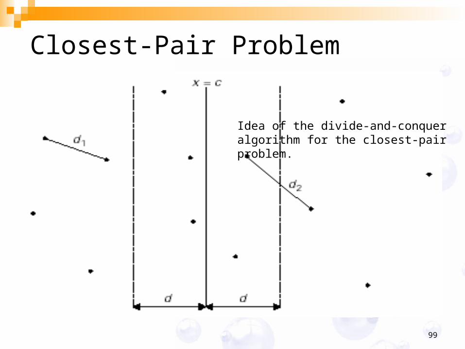
Closest-Pair Problem
Idea of the divide-and-conquer algorithm for the closest-pair problem.
100
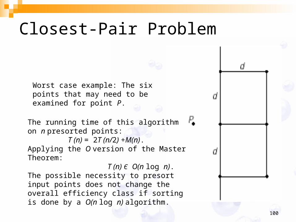
Closest-Pair Problem
Worst case example: The six points that may need to be examined for point P.
The running time of this algorithm on n presorted points: T (n) = 2T (n/2) +M(n).Applying the O version of the Master Theorem: T (n) Є O(n log n). The possible necessity to presort input points does not change the overall efficiency class if sorting is done by a O(n log n) algorithm.
101
ITS033Topic 01Topic 01 -- Problems & Algorithmic Problem SolvingProblems & Algorithmic Problem SolvingTopic 02Topic 02 – Algorithm Representation & Efficiency Analysis – Algorithm Representation & Efficiency AnalysisTopic 03Topic 03 - State Space of a problem - State Space of a problemTopic 04Topic 04 - Brute Force Algorithm - Brute Force AlgorithmTopic 05 - Divide and ConquerTopic 05 - Divide and ConquerTopic 06Topic 06 -- Decrease and ConquerDecrease and ConquerTopic 07Topic 07 - Dynamics Programming - Dynamics ProgrammingTopic 08Topic 08 -- Transform and ConquerTransform and ConquerTopic 09Topic 09 - Graph Algorithms - Graph AlgorithmsTopic 10Topic 10 - Minimum Spanning Tree - Minimum Spanning TreeTopic 11Topic 11 - Shortest Path Problem - Shortest Path ProblemTopic 12Topic 12 - Coping with the Limitations of Algorithms Power - Coping with the Limitations of Algorithms Power
http://www.siit.tu.ac.th/bunyarit/its033.phphttp://www.siit.tu.ac.th/bunyarit/its033.phpand and http://www.vcharkarn.com/vlesson/showlesson.php?lessonid=7http://www.vcharkarn.com/vlesson/showlesson.php?lessonid=7

102
End of Chapter 4
Thank you!