Analisa Perbandingan Metode Hierarchical Clustering dan Nonhierarchical Clustering
Upload
maya-sidneyCategory
view
219download
3
1
CSE 980: Data Mining
Lecture 16: Hierarchical Clustering

2
Hierarchical Clustering
Produces a set of nested clusters organized as a hierarchical tree
Can be visualized as a dendrogram– A tree like diagram that records the sequences of
merges or splits
1 3 2 5 4 60
0.05
0.1
0.15
0.2
1
2
3
4
5
6
1
23 4
5

3
Strengths of Hierarchical Clustering
Do not have to assume any particular number of clusters– Any desired number of clusters can be obtained by
‘cutting’ the dendogram at the proper level
They may correspond to meaningful taxonomies– Example in biological sciences (e.g., animal kingdom,
phylogeny reconstruction, …)

4
Hierarchical Clustering
Two main types of hierarchical clustering– Agglomerative:
Start with the points as individual clusters At each step, merge the closest pair of clusters until only one cluster (or k clusters) left
– Divisive: Start with one, all-inclusive cluster At each step, split a cluster until each cluster contains a point (or there are k clusters)
Traditional hierarchical algorithms use a similarity or distance matrix
– Merge or split one cluster at a time

5
MST: Divisive Hierarchical Clustering
Build MST (Minimum Spanning Tree)– Start with a tree that consists of any point
– In successive steps, look for the closest pair of points (p, q) such that one point (p) is in the current tree but the other (q) is not
– Add q to the tree and put an edge between p and q

6
Agglomerative Clustering Algorithm
More popular hierarchical clustering technique
Basic algorithm is straightforward1. Compute the proximity matrix
2. Let each data point be a cluster
3. Repeat
4. Merge the two closest clusters
5. Update the proximity matrix
6. Until only a single cluster remains
Key operation is the computation of the proximity of two clusters
– Different approaches to defining the distance between clusters distinguish the different algorithms

7
Starting Situation
Start with clusters of individual points and a proximity matrix
p1
p3
p5
p4
p2
p1 p2 p3 p4 p5 . . .
.
.
. Proximity Matrix
...p1 p2 p3 p4 p9 p10 p11 p12

8
Intermediate Situation
After some merging steps, we have some clusters
C1
C4
C2 C5
C3
C2C1
C1
C3
C5
C4
C2
C3 C4 C5
Proximity Matrix
...p1 p2 p3 p4 p9 p10 p11 p12
9
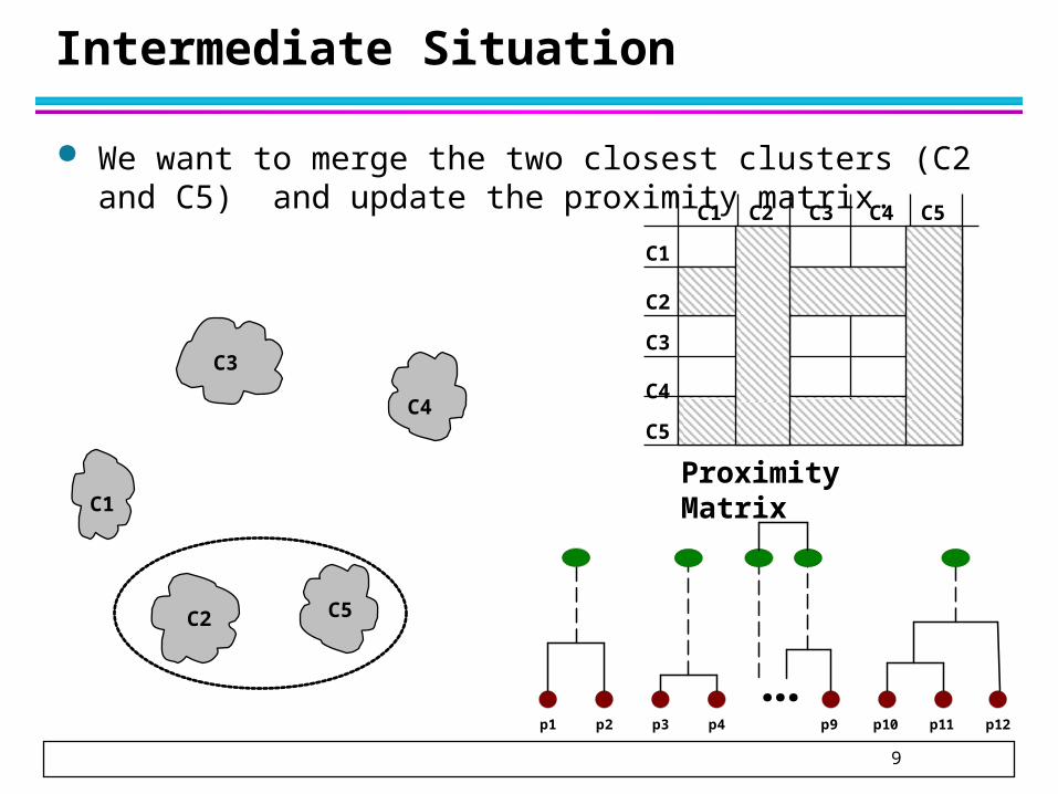
Intermediate Situation
We want to merge the two closest clusters (C2 and C5) and update the proximity matrix.
C1
C4
C2 C5
C3
C2C1
C1
C3
C5
C4
C2
C3 C4 C5
Proximity Matrix
...p1 p2 p3 p4 p9 p10 p11 p12

10
After Merging
The question is “How do we update the proximity matrix?”
C1
C4
C2 U C5
C3? ? ? ?
?
?
?
C2 U C5C1
C1
C3
C4
C2 U C5
C3 C4
Proximity Matrix
...p1 p2 p3 p4 p9 p10 p11 p12

11
How to Define Inter-Cluster Similarity
p1
p3
p5
p4
p2
p1 p2 p3 p4 p5 . . .
.
.
.
Similarity?
MIN MAX Group Average Distance Between Centroids Other methods driven by an objective
function– Ward’s Method uses squared error
Proximity Matrix

12
How to Define Inter-Cluster Similarity
p1
p3
p5
p4
p2
p1 p2 p3 p4 p5 . . .
.
.
.Proximity Matrix
MIN MAX Group Average Distance Between Centroids Other methods driven by an objective
function– Ward’s Method uses squared error

13
How to Define Inter-Cluster Similarity
p1
p3
p5
p4
p2
p1 p2 p3 p4 p5 . . .
.
.
.Proximity Matrix
MIN MAX Group Average Distance Between Centroids Other methods driven by an objective
function– Ward’s Method uses squared error

14
How to Define Inter-Cluster Similarity
p1
p3
p5
p4
p2
p1 p2 p3 p4 p5 . . .
.
.
.Proximity Matrix
MIN MAX Group Average Distance Between Centroids Other methods driven by an objective
function– Ward’s Method uses squared error

15
How to Define Inter-Cluster Similarity
p1
p3
p5
p4
p2
p1 p2 p3 p4 p5 . . .
.
.
.Proximity Matrix
MIN MAX Group Average Distance Between Centroids Other methods driven by an objective
function– Ward’s Method uses squared error

16
Cluster Similarity: MIN or Single Link
Similarity of two clusters is based on the two most similar (closest) points in the different clusters– Determined by one pair of points, i.e., by one link in
the proximity graph.
I1 I2 I3 I4 I5I1 1.00 0.90 0.10 0.65 0.20I2 0.90 1.00 0.70 0.60 0.50I3 0.10 0.70 1.00 0.40 0.30I4 0.65 0.60 0.40 1.00 0.80I5 0.20 0.50 0.30 0.80 1.00 1 2 3 4 5

17
Hierarchical Clustering: MIN
Nested Clusters Dendrogram
1
2
3
4
5
6
1
2
3
4
5
3 6 2 5 4 10
0.05
0.1
0.15
0.2

18
Strength of MIN
Original Points Two Clusters
• Can handle non-elliptical shapes

19
Limitations of MIN
Original Points Two Clusters
• Sensitive to noise and outliers

20
Cluster Similarity: MAX or Complete Linkage
Similarity of two clusters is based on the two least similar (most distant) points in the different clusters– Determined by all pairs of points in the two clusters
I1 I2 I3 I4 I5I1 1.00 0.90 0.10 0.65 0.20I2 0.90 1.00 0.70 0.60 0.50I3 0.10 0.70 1.00 0.40 0.30I4 0.65 0.60 0.40 1.00 0.80I5 0.20 0.50 0.30 0.80 1.00 1 2 3 4 5

21
Hierarchical Clustering: MAX
Nested Clusters Dendrogram
3 6 4 1 2 50
0.05
0.1
0.15
0.2
0.25
0.3
0.35
0.4
1
2
3
4
5
6
1
2 5
3
4

22
Strength of MAX
Original Points Two Clusters
• Less susceptible to noise and outliers

23
Limitations of MAX
Original Points Two Clusters
•Tends to break large clusters
•Biased towards globular clusters

24
Cluster Similarity: Group Average
Proximity of two clusters is the average of pairwise proximity between points in the two clusters.
Need to use average connectivity for scalability since total proximity favors large clusters
||Cluster||Cluster
)p,pproximity(
)Cluster,Clusterproximity(ji
ClusterpClusterp
ji
jijjii
I1 I2 I3 I4 I5I1 1.00 0.90 0.10 0.65 0.20I2 0.90 1.00 0.70 0.60 0.50I3 0.10 0.70 1.00 0.40 0.30I4 0.65 0.60 0.40 1.00 0.80I5 0.20 0.50 0.30 0.80 1.00 1 2 3 4 5

25
Hierarchical Clustering: Group Average
Nested Clusters Dendrogram
3 6 4 1 2 50
0.05
0.1
0.15
0.2
0.25
1
2
3
4
5
6
1
2
5
3
4

26
Hierarchical Clustering: Group Average
Compromise between Single and Complete Link
Strengths– Less susceptible to noise and outliers
Limitations– Biased towards globular clusters

27
Hierarchical Clustering: Comparison
Group Average
Ward’s Method
1
2
3
4
5
61
2
5
3
4
MIN MAX
1
2
3
4
5
61
2
5
34
1
2
3
4
5
61
2 5
3
41
2
3
4
5
6
12
3
4
5

28
Hierarchical Clustering: Time and Space
requirements
O(N2) space since it uses the proximity matrix. – N is the number of points.
O(N3) time in many cases– There are N steps and at each step the size, N2,
proximity matrix must be updated and searched
– Complexity can be reduced to O(N2 log(N) ) time for some approaches

29
Hierarchical Clustering: Problems and
Limitations
Once a decision is made to combine two clusters, it cannot be undone
No objective function is directly minimized
Different schemes have problems with one or more of the following:– Sensitivity to noise and outliers
– Difficulty handling different sized clusters and convex shapes
– Breaking large clusters