1 7. What to Optimize? In this session: 1.Can one do better by optimizing something else?...

SPF workshop February 2014, UBCO 1

7. What to Optimize?

In this session:1. Can one do better by optimizing something else?2. Likelihood, not LS?3. Using a handful of likelihood functions.

CH1. What is what CH2. A simple SPF CH3. EDA CH4. Curve fitting CH5. A first SPF CH6: Which fit is fitter CH7: Choosing the objective function CH8: Theoretical stuff Ch9: Adding variables CH10. Choosing a model equation


Perhaps the fit was bad because:• The function is not good• Important traits are missing• The objective function is not appropriate

later

Now

The two common methods: Least Squares Maximum Likelihood

Carl Friedrich Gauss1777-1855

Sir Ronald Fisher1890-1962

1β

0XβμE


Introducing ‘Likelihood’

In statistics, maximum-likelihood estimation (MLE) is a method of estimating the parameters of a statistical model. When applied to a data set and given a statistical model, maximum-likelihood estimation provides estimates for the model's parameters.From Wikipedia

Popular in SPF modeling

http://en.wikipedia.org/wiki/Estimator

http://en.wikipedia.org/wiki/Parameter

http://en.wikipedia.org/wiki/Statistical_model

http://en.wikipedia.org/wiki/Statistical_model

http://en.wikipedia.org/wiki/Estimator


Year 1 2 3 4Crashes 1 7 4 0

What is the probability of 1, 7, 4, 0 if μ=2.0 crashes/year?

Open #9. ‘Likelihood functions’ on ‘Poisson’ workpage

Example 1: Get the ML estimate of a m

5

The likelihood of μ=4.0

The likelihood of μ=2.0

The ‘Likelihood Function’

ℒ(.) will be used to denote a likelihood function. The dot in the parenthesis is a placeholder for parameters. Thus, e.g., ℒ(μ) is the is the likelihood function of μ.


Computing likelihood at very many μ’s we would see a smooth curve - the ‘likelihood function’.

0 3 6 90E+00

1E-05

2E-05

3E-05

Means

Likel

ihoo

d

Probability to observe 1, 7,4 and 0 accidents

The m at whichObserving1 & 7 &4 & 0 is most probable


The parameter value at which the likelihood function has its peak is the ‘Maximum Likelihood’ (ML) estimate of that parameter.

It is not the most probable value of the parameter.

It is the parameter value at which the observations are most probable.


Return to #9 on the ‘Poisson ML’ workpage

The ‘Target’ cell The ‘By Changing’ cell

Use ‘Solver’

With the 1, 7, 4, 0 crash record, which μ is most likely?

Show that ML estimate of m is 3.00.


Example 2: What distribution fits the data?

Number of drivers out of 29531 who, during 1931-1936 had 1 accident.

Continue now to the ‘Does the Poisson fit’ workpage.

The Data

If all drivers had the same m then one would expect n(k) to be consistent with the Poisson distribution. Is it?

SPF workshop February 2014, UBCO10

Here the Poisson predicts too few crashes

0 1 2 3 4 5 6 70.000

0.500

1.000

1.500

If Poisson was a good fit

Answer: ....

11

What distribution does fit the data?

Continue to the ‘NegBin ML Empty’ workpage in #9.

NB applies to populations of units where each unit may

have a different m and the m’s are

Gamma distributed

Poisson applies to population of units that all have the same

m

12

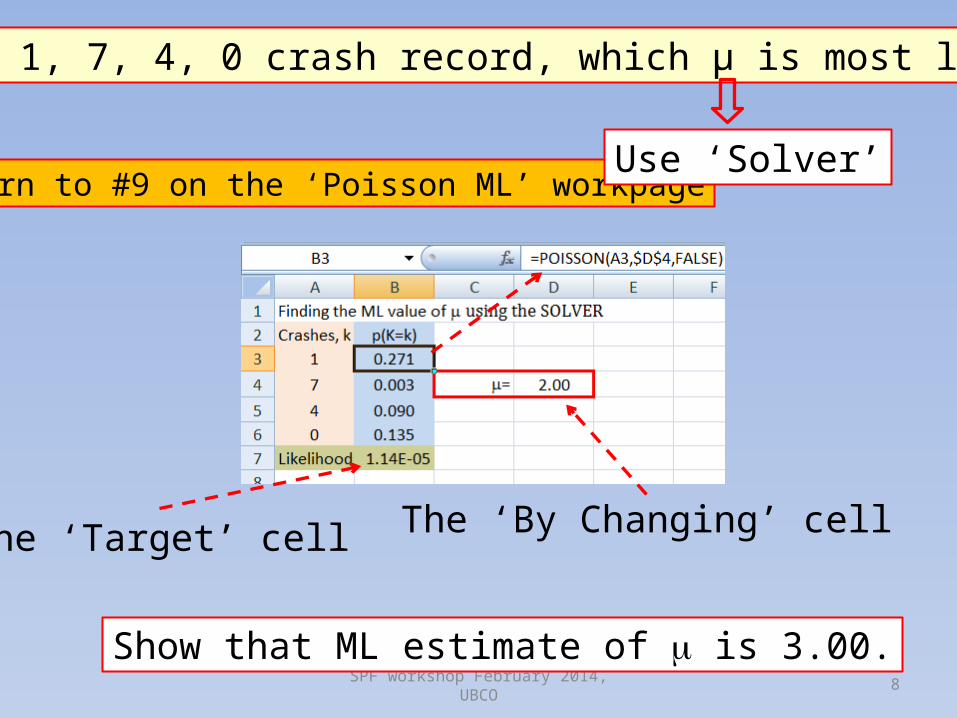
1781-18401817-1951PሺK= kሻ= μke−μk!

Parameters to be estimated

Will NB fit the data?


Question 1: What are the ML estimates of ‘a’ and ‘b’?(both must be positive)

Question 2: With these ‘a’ and ‘b’ how good is the correspondence between the observed and fitted n(k)


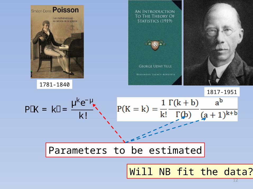
The likelihood function is the product of many small probabilities. To avoid computational difficulties we use the log-likelihood ‘product’ replaced by ‘sum’.

Initial guesses

Preparing the likelihood function for Solver


The probability than n(k) units have k accidents is P(K=k)n(k)

The log-likelihood is the sum over all k of n(k)ln[P(K=k)]

Now we are ready to estimate ‘a’ and ‘b’

B*C


‘a’ and ‘b’ must be non-negative

ML estimates

Does this NB fit the data?


Was the NB assumption for populations reasonable?

Numbers expected if NB and parameters both were true.

(By method of moments in 1.4 we got 3.55 and 0.85)


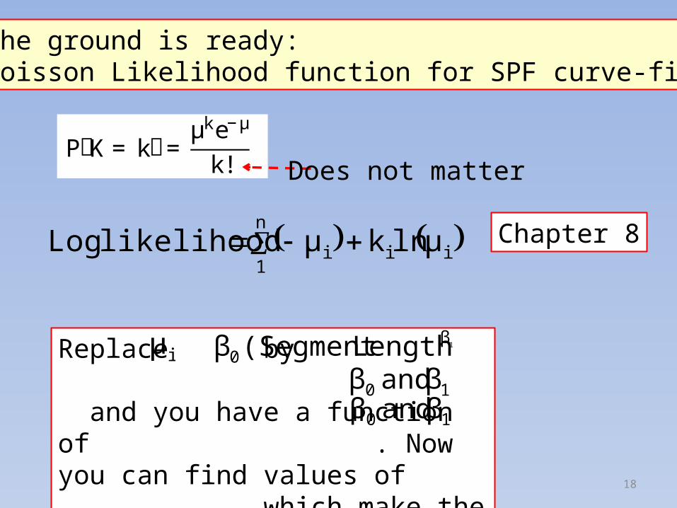
Now the ground is ready:The Poisson Likelihood function for SPF curve-fitting

n

1iii μlnkμlikelihoodLog Chapter 8

Replace by and you have a function of . Now you can find values of which make the log-likelihood largest.

iμ 1β

0 Length)(Segmentβ

10 βandβ

PሺK= kሻ= μke−μk!

10 βandβ

Does not matter

19

The C-F spreadsheet for Poisson likelihood function.

Go to: #10.Poisson fit (Full).xlsx on ‘Poisson’ workpage

Our model equation (for now)

Sum of log-likelihoods

n

1iii μlnkμlikelihoodLog

Formula:=-E8+D8*LN(E8), copy down

Very similar to OLS,No point in CURE

SOLVER solution

Click


The Poisson L-F solves the ‘equal variances’ problem.However, it has a problem of its own – no overdispersion.

The Negative Binomial Likelihood Function

To illustrate, 91 of 5323 segments are 0.01 miles long.For these,

Sample Variance of accident counts =0.114, Sample Mean of accident counts =0.098.

If Poisson, Variance=MeanIf Variance>Mean, Overdispersion, not Poisson


(Sam

ple

varia

nce)

/(Sa

mpl

e M

ean)

Segment Length [miles]

50 segment length bins

If Poisson


The NB Likelihood Function continued

Poisson Negative Binomial

Crash Counts for each unit are Poisson distributed

Crash Counts for each unit are Poisson distributed

Units with the same traits in the model equation have

the same μ

Units with the same traits in the model equation have

μ’s that comes from a Gamma distribution

Assumptions: Common and Different

24

• The Gamma pdf can take on a variety of shapes.• Limitations.

E{μ}=b/a, VAR{μ}=(E{μ})2/b

For many populations NB fits. Ergo: Gamma is often OK.


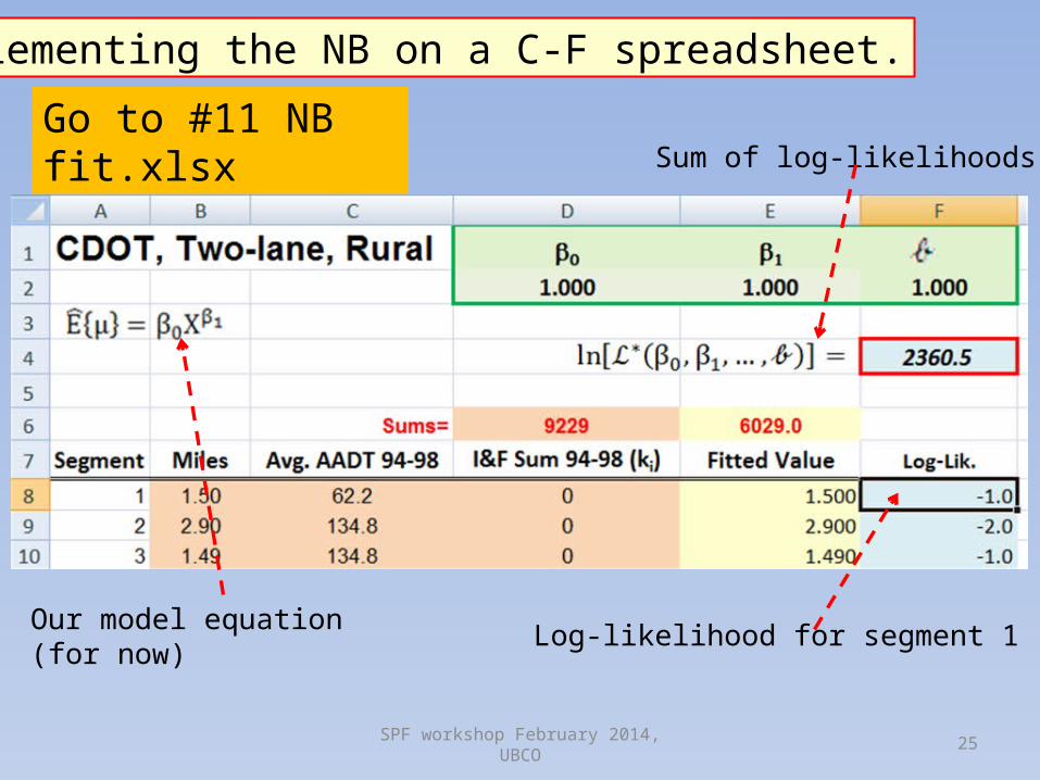
Go to #11 NB fit.xlsx

Our model equation (for now)

Implementing the NB on a C-F spreadsheet.

Log-likelihood for segment 1

Sum of log-likelihoods

26

lnሾℒ∗ሺβ0,β1,…,𝒷ሻሿ== [lnΓሺki + 𝒷Liሻ− lnΓሺ𝒷Liሻ

ni=1 + 𝒷Li lnሺbLiሻ+ ki ln൫Eሼμiሽ൯

−ሺ𝒷Li + kiሻln(𝒷Li + E {μi})] Details in text

Modifying the Poisson C-F spreadsheet to NB

=IF(OR(B8<=0,C8<=0,E8<=0),0,GAMMALN(D8+$G$2*B8)-GAMMALN($G$2*B8)+$G$2*B8*LN($G$2*B8)+D8*LN(E8)-($G$2*B8+D8)*LN($G$2*B8+E8))

Add cell for new parameter

27

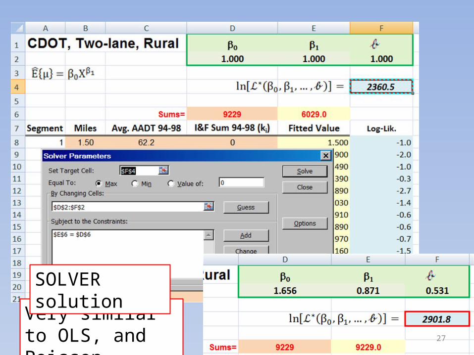
Very similar to OLS, and Poisson

SOLVER solution


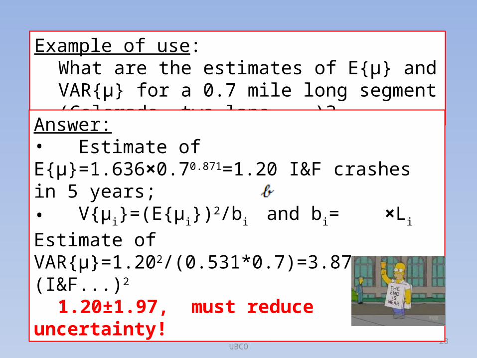
Example of use: What are the estimates of E{μ} and VAR{μ} for a 0.7 mile long segment (Colorado, two-lane,...)?

Answer:• Estimate of E{μ}=1.636×0.70.871=1.20 I&F crashes in 5 years;• V{μi}=(E{μi})2/bi and bi= ×LiEstimate of VAR{μ}=1.202/(0.531*0.7)=3.87 (I&F...)2

1.20±1.97, must reduce uncertainty!


In this session we asked: What to Optimize?Traditionally:1. Minimize (weighted) SSD2. Maximize LikelihoodBoth are motivated by focus on parameters

When the focus is on ‘How to predict well’, other criteria emerge:1. Minimize absolute deviations2. Minimize Total Absolute Bias3. Minimize , etc. In lecture notes.

2χ


Summary for Chapter 7.

1. Instead of minimizing SSD (which gave poor fits), we asked whether fit is improved by maximizing likelihood;

2. Likelihood was explained and illustrated;3. To write a likelihood function one must make

assumptions. The assumptions behind the Poisson and NB likelihoods were discussed;

4. We used the Poisson likelihood function. The fit was not improved.

5. One of the assumptions behind the Poisson likelihood is not realistic. The NB likelihood function removes the blemish.


6. The estimate of the shape parameter ‘b’ is needed for tasks such as blackspot identification and EB safety estimation;

7. The fit is still not very good. Can it be improved by using a better model equation?

1 7. What to Optimize? In this session: 1.Can one do better by optimizing something else?...

Documents

Transcript of 1 7. What to Optimize? In this session: 1.Can one do better by optimizing something else?...