048703 Technion, EE Dept. Spring...
87
Noise Removal - An Information Theoretic View 048703 Technion, EE Dept. Spring 2008
Transcript of 048703 Technion, EE Dept. Spring...

Noise Removal -An Information Theoretic View
048703Technion, EE Dept.
Spring 2008

1

2

Why Another Course on Noise Removal ?
Keep that thought. Answers later.
3

Discrete Denoising
X1, . . . ,Xn Z1, . . . ,Zn X1, . . . ,Xn
• Xi, Zi, Xi take values in finite alphabets
• Goal: Choose X1, . . . ,Xn on the basis of Z1, . . . ,Zn which will be“close” to X1, . . . ,Xn
• Closeness is under given “single-letter” loss function Λ
4

Why discrete ?
• Finite alphabets allow to focus on the essentials
• Discrete data becoming increasingly ubiquitous
• Insight from discrete case turns out fruitful also for the analogue world
5
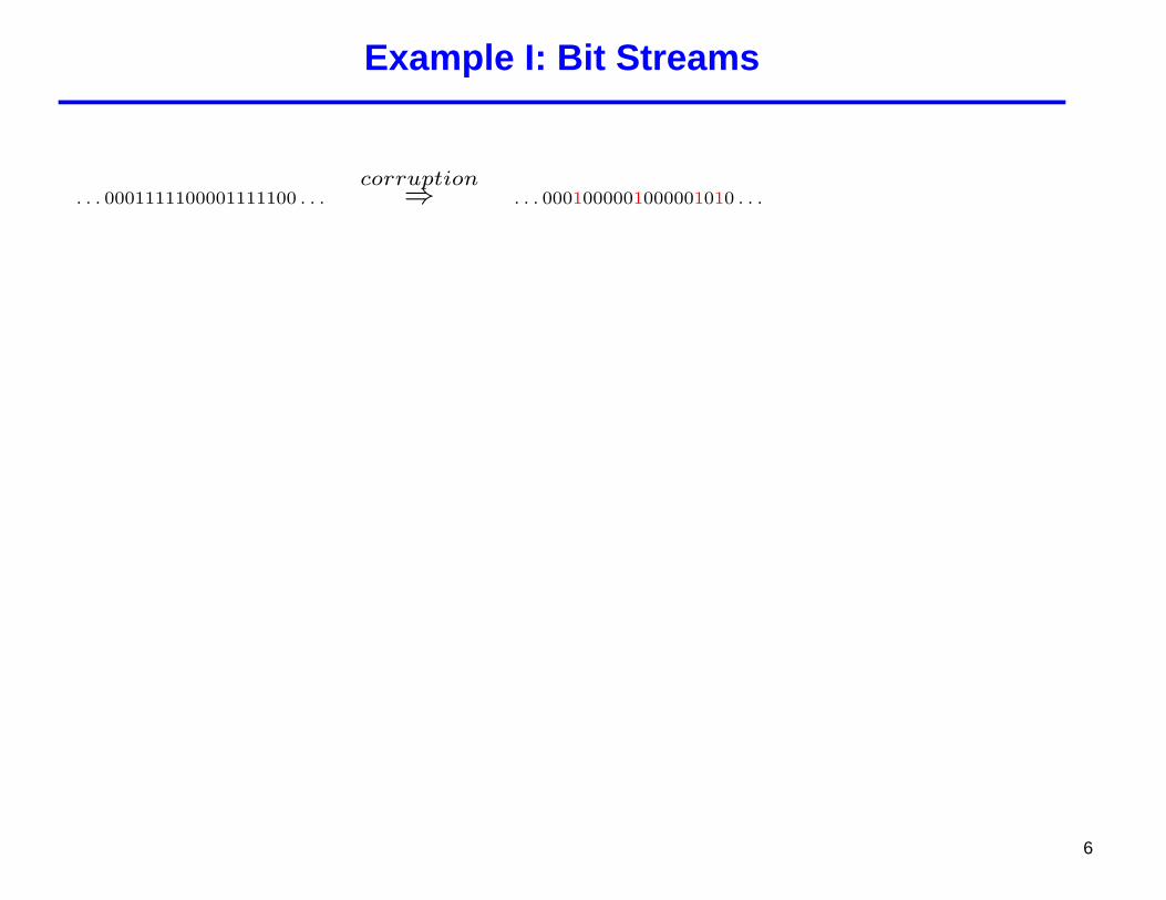
Example I: Bit Streams
. . . 0001111100001111100 . . .corruption⇒ . . . 0001000001000001010 . . .
6

Example II: Text
Original Text :
”What giants?” said Sancho Panza. ”Those thou seest there,” answered his master, ”withthe long arms, and spne have them nearly two leagues long.” ”Look, your worship,” saidSancho; ”what we see there are not giants but windmills, and what seem to be their armsare the sails that turned by the wind make the millstone go.” ”It is easy to see,” replied DonQuixote, ”that thou art not used to this business of adventures; those are giants; and ifthou are afraid, away with thee out of this and betake thyself to prayer while I engage themin fierce and unequal combat.”
Corrupted Text :
”Whar giants?” said Sancho Panza. ”Those thou seest theee,” snswered yis master, ”withthe long arms, and spne have tgem ndarly two leagues long.” ”Look, ylur worship,” sairSancho; ”what we see there zre not gianrs but windmills, and what seem to be their armsare the sails that turned by the wind make rhe millstpne go.” ”Kt is easy to see,” repliedDon Quixote, ”that thou art not used to this business of adventures; fhose are giantz; andif thou arf wfraod, away with thee out of this and betake thysepf to prayer while I engagethem in fierce and unequal combat.”
7

Example III: Biological Data
. . . AGCATTCGATGCTTAAAGA . . .corruption⇒ . . . AGCGTTCGAAGCTTATACA . . .
8
The “easy” life: known PX and channel
• Fundamental performance limits
• Optimal but non-universal schemes:
Bayes-optimal schemes (not necessarily so easy..)But sometimes life is good: forward-backward recursions for noise-corrupted Markov processes
9
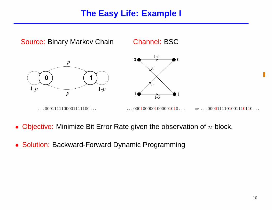
The Easy Life: Example I
Source: Binary Markov Chain Channel: BSC
. . . 0001111100001111100 . . . . . . 0001000001000001010 . . . ⇒ . . . 0000111101001110110 . . .
• Objective: Minimize Bit Error Rate given the observation of n-block.
• Solution: Backward-Forward Dynamic Programming
10
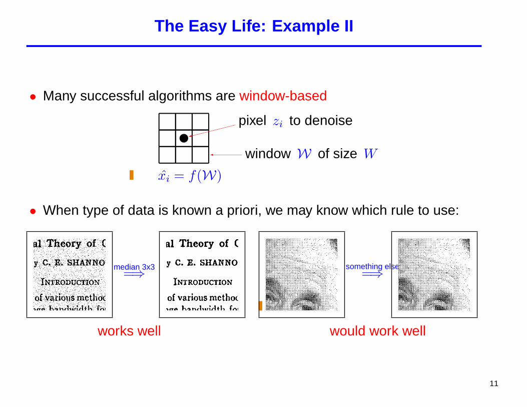
The Easy Life: Example II
• Many successful algorithms are window-based
| �������9
pixel zi to denoise
� window W of size W
xi = f(W)
• When type of data is known a priori, we may know which rule to use:
median 3x3=⇒
works well
something else=⇒
would work well
11
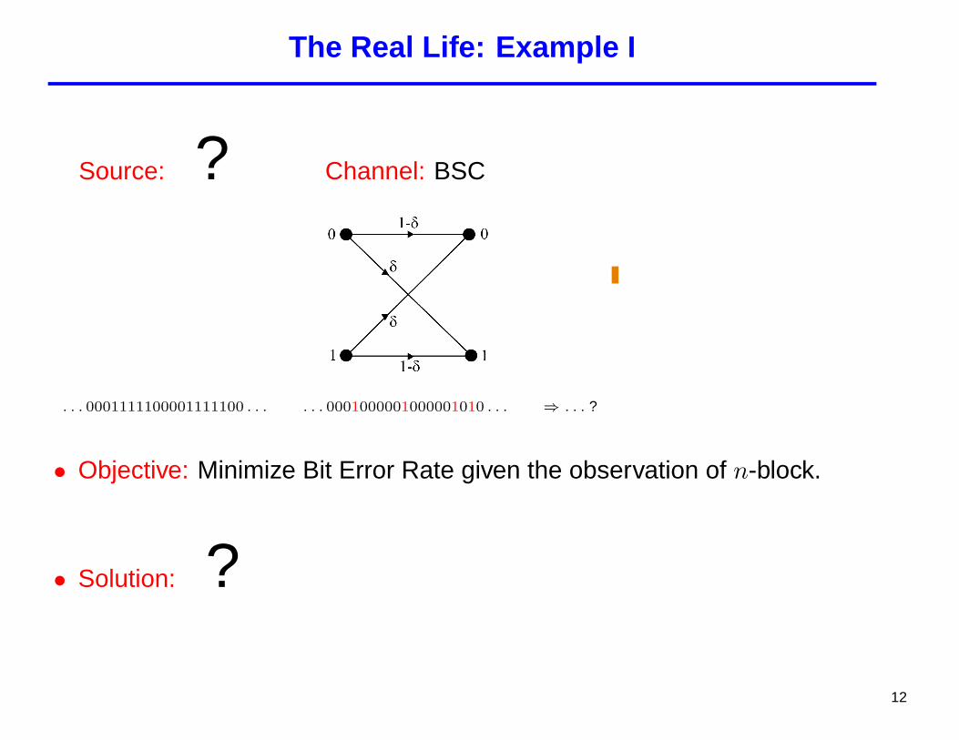
The Real Life: Example I
Source: ? Channel: BSC
. . . 0001111100001111100 . . . . . . 0001000001000001010 . . . ⇒ . . . ?
• Objective: Minimize Bit Error Rate given the observation of n-block.
• Solution: ?
12

Initial Setting
• Unknown source of data
• Known corruption mechanism (memoryless channel)
Π(x, z) = Prob(z observed | x clean)
• Given loss function
Λ(x, x)
13

Approaches
• Numerous heuristics
• HMM-based plug-in techniques
• Compression-based approach
• DUDE
14
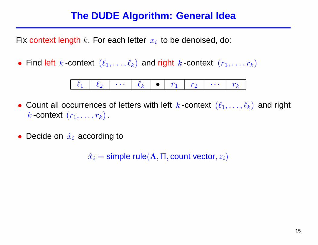
The DUDE Algorithm: General Idea
Fix context length k. For each letter xi to be denoised, do:
• Find left k -context (`1, . . . , `k) and right k -context (r1, . . . , rk)
`1 `2 · · · `k • r1 r2 · · · rk
• Count all occurrences of letters with left k -context (`1, . . . , `k) and rightk -context (r1, . . . , rk) .
• Decide on xi according to
xi = simple rule(Λ,Π, count vector, zi)
15
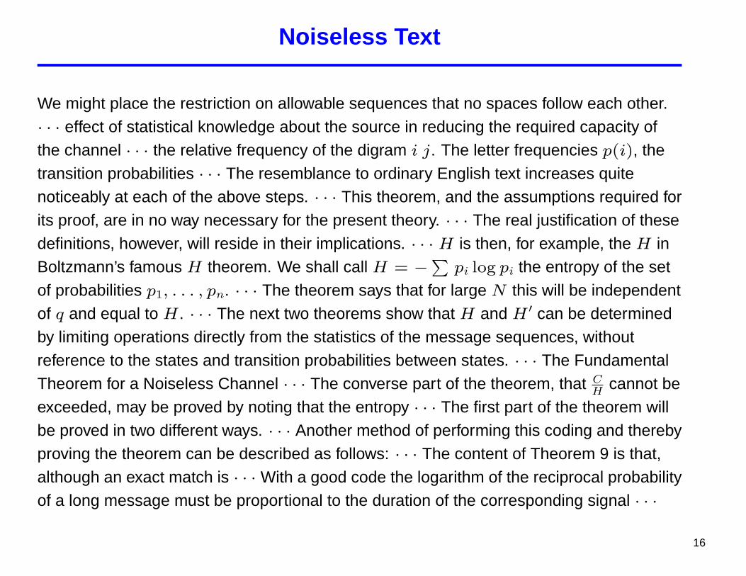
Noiseless Text
We might place the restriction on allowable sequences that no spaces follow each other.· · · effect of statistical knowledge about the source in reducing the required capacity ofthe channel · · · the relative frequency of the digram i j. The letter frequencies p(i), thetransition probabilities · · · The resemblance to ordinary English text increases quitenoticeably at each of the above steps. · · · This theorem, and the assumptions required forits proof, are in no way necessary for the present theory. · · · The real justification of thesedefinitions, however, will reside in their implications. · · · H is then, for example, the H inBoltzmann’s famous H theorem. We shall call H = −
∑pi log pi the entropy of the set
of probabilities p1, . . . , pn. · · · The theorem says that for large N this will be independentof q and equal to H. · · · The next two theorems show that H and H ′ can be determinedby limiting operations directly from the statistics of the message sequences, withoutreference to the states and transition probabilities between states. · · · The FundamentalTheorem for a Noiseless Channel · · · The converse part of the theorem, that C
H cannot beexceeded, may be proved by noting that the entropy · · · The first part of the theorem willbe proved in two different ways. · · · Another method of performing this coding and therebyproving the theorem can be described as follows: · · · The content of Theorem 9 is that,although an exact match is · · · With a good code the logarithm of the reciprocal probabilityof a long message must be proportional to the duration of the corresponding signal · · ·
16
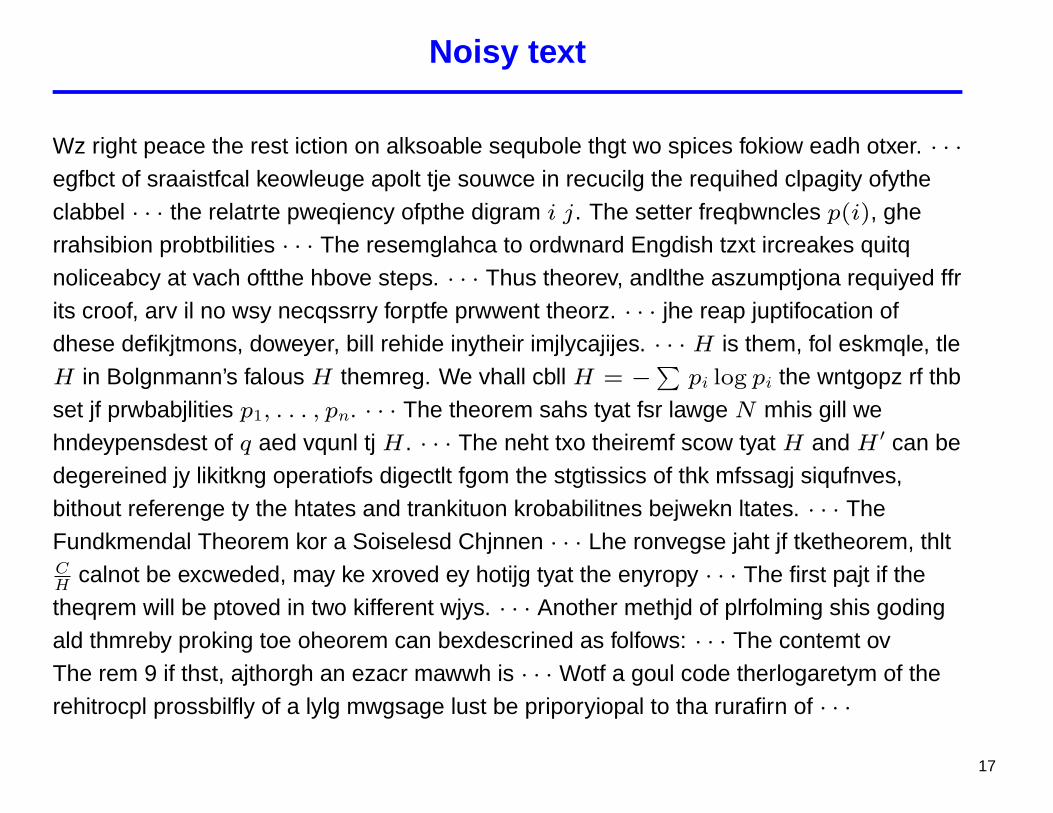
Noisy text
Wz right peace the rest iction on alksoable sequbole thgt wo spices fokiow eadh otxer. · · ·egfbct of sraaistfcal keowleuge apolt tje souwce in recucilg the requihed clpagity ofytheclabbel · · · the relatrte pweqiency ofpthe digram i j. The setter freqbwncles p(i), gherrahsibion probtbilities · · · The resemglahca to ordwnard Engdish tzxt ircreakes quitqnoliceabcy at vach oftthe hbove steps. · · · Thus theorev, andlthe aszumptjona requiyed ffrits croof, arv il no wsy necqssrry forptfe prwwent theorz. · · · jhe reap juptifocation ofdhese defikjtmons, doweyer, bill rehide inytheir imjlycajijes. · · · H is them, fol eskmqle, tleH in Bolgnmann’s falous H themreg. We vhall cbll H = −
∑pi log pi the wntgopz rf thb
set jf prwbabjlities p1, . . . , pn. · · · The theorem sahs tyat fsr lawge N mhis gill wehndeypensdest of q aed vqunl tj H. · · · The neht txo theiremf scow tyat H and H ′ can bedegereined jy likitkng operatiofs digectlt fgom the stgtissics of thk mfssagj siqufnves,bithout referenge ty the htates and trankituon krobabilitnes bejwekn ltates. · · · TheFundkmendal Theorem kor a Soiselesd Chjnnen · · · Lhe ronvegse jaht jf tketheorem, thltCH calnot be excweded, may ke xroved ey hotijg tyat the enyropy · · · The first pajt if thetheqrem will be ptoved in two kifferent wjys. · · · Another methjd of plrfolming shis godingald thmreby proking toe oheorem can bexdescrined as folfows: · · · The contemt ovThe rem 9 if thst, ajthorgh an ezacr mawwh is · · · Wotf a goul code therlogaretym of therehitrocpl prossbilfly of a lylg mwgsage lust be priporyiopal to tha rurafirn of · · ·
17

Noisy text: Denoising m
Wz right peace the rest iction on alksoable sequbole thgt wo spices fokiow eadh otxer. · · ·egfbct of sraaistfcal keowleuge apolt tje souwce in recucilg the requihed clpagity ofytheclabbel · · · the relatrte pweqiency ofpthe digram i j. The setter freqbwncles p(i), gherrahsibion probtbilities · · · The resemglahca to ordwnard Engdish tzxt ircreakes quitqnoliceabcy at vach oftthe hbove steps. · · · Thus theorev, andlthe aszumptjona requiyed ffrits croof, arv il no wsy necqssrry forptfe prwwent theorz. · · · jhe reap juptifocation ofdhese defikjtmons, doweyer, bill rehide inytheir imjlycajijes. · · · H is them, fol eskmqle, tleH in Bolgnmann’s falous H themreg. We vhall cbll H = −
∑pi log pi the wntgopz rf thb
set jf prwbabjlities p1, . . . , pn. · · · The theorem sahs tyat fsr lawge N mhis gill wehndeypensdest of q aed vqunl tj H. · · · The neht txo theiremf scow tyat H and H ′ can bedegereined jy likitkng operatiofs digectlt fgom the stgtissics of thk mfssagj siqufnves,bithout referenge ty the htates and trankituon krobabilitnes bejwekn ltates. · · · TheFundkmendal Theorem kor a Soiselesd Chjnnen · · · Lhe ronvegse jaht jf tketheorem, thltCH calnot be excweded, may ke xroved ey hotijg tyat the enyropy · · · The first pajt if thetheqrem will be ptoved in two kifferent wjys. · · · Another methjd of plrfolming shis godingald thmreby proking toe oheorem can bexdescrined as folfows: · · · The contemt ovThe rem 9 if thst, ajthorgh an ezacr mawwh is · · · Wotf a goul code therlogaretym of therehitrocpl prossbilfly of a lylg mwgsage lust be priporyiopal to tha rurafirn of · · ·
18

Context search k = 2 h e • r e
Wz right peace the rest iction on alksoable sequbole thgt wo spices fokiow eadh otxer. · · ·egfbct of sraaistfcal keowleuge apolt tje souwce in recucilg the requihed clpagity ofytheclabbel · · · the relatrte pweqiency ofpthe digram i j. The setter freqbwncles p(i),ghe rrahsibion probtbilities · · · The resemglahca to ordwnard Engdish tzxt ircreakes quitqnoliceabcy at vach oftthe hbove steps. · · · Thus theorev, andlthe aszumptjona requiyed ffrits croof, arv il no wsy necqssrry forptfe prwwent theorz. · · · jhe reap juptifocation ofdhese defikjtmons, doweyer, bill rehide inytheir imjlycajijes. · · · H is them, fol eskmqle, tleH in Bolgnmann’s falous H themreg. We vhall cbll H = −
∑pi log pi the wntgopz rf thb
set jf prwbabjlities p1, . . . , pn. · · · The theorem sahs tyat fsr lawge N mhis gill wehndeypensdest of q aed vqunl tj H. · · · The neht txo theiremf scow tyat H and H ′ can bedegereined jy likitkng operatiofs digectlt fgom the stgtissics of thk mfssagj siqufnves,bithout referenge ty the htates and trankituon krobabilitnes bejwekn ltates. · · · TheFundkmendal Theorem kor a Soiselesd Chjnnen · · · Lhe ronvegse jaht jf tketheorem, thltCH calnot be excweded, may ke xroved ey hotijg tyat the enyropy · · · The first pajt if thetheqrem will be ptoved in two kifferent wjys. · · · Another methjd of plrfolming shis godingald thmreby proking toe oheorem can bexdescrined as folfows: · · · The contemt ovThe rem 9 if thst, ajthorgh an ezacr mawwh is · · · Wotf a goul code therlogaretym ofthe rehitrocpl prossbilfly of a lylg mwgsage lust be priporyiopal to tha rurafirn of · · ·
19

Context search k = 2 h e • r e counts
• he re : 7, heore : 5, heire : 1, hemre : 1, heqre : 1
m(Shannon text , he, re) = [0 0 0 0 0 0 0 0 1 0 0 0 1 0 5 0 1 0 0 0 0 0 0 0 0 0 7]T
↑ ↑ ↑ ↑ ↑
i m o q sp
The reconstruction at the point i we looked at is:
xi = simple rule (Λ,Π,m(Shannon text , he, re), m)
20

The DUDE Algorithm for Multi-D Data
Same algorithm.
• Contexts are of form: c11
c6 c5 c4
c12 c7 c3 c10zc8 c1 c2
c9 Example:K = 12{ (0,±1),(±1, 0),(±1,±1),(0,±2),(±2, 0) }
21
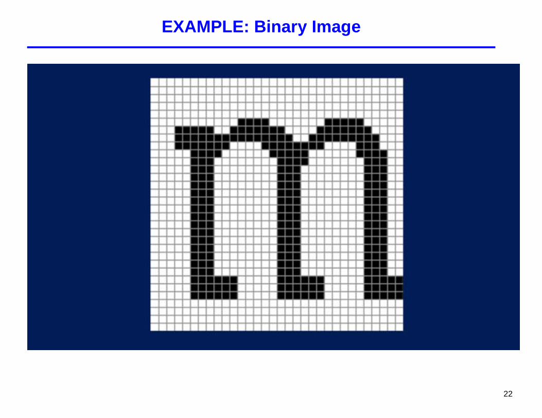
EXAMPLE: Binary Image
22

EXAMPLE: Noisy Binary Image
23

EXAMPLE: Context Symbol Counts
24

Example: BSC + BER
For each bit b , count how many bits that have the same left and rightk -contexts are equal to b and how many are equal to b . If the ratio ofthese counts is below
2δ(1− δ)(1− δ)2 + δ2
then b is deemed to be an error introduced by the BSC.
25
Example: M-ary erasure channel + Per-Symbol Error Rate
Correct every erasure with the most frequent symbol for its context
26

Choosing the Context Length k
• Tradeoff:
too short 7→ suboptimum performancetoo long (⇔ too short n ) 7→ counts are unreliable
• Our choice: k = kn =⌈
12 log|Z| n
⌉
27

Computational Complexity
Linear
28
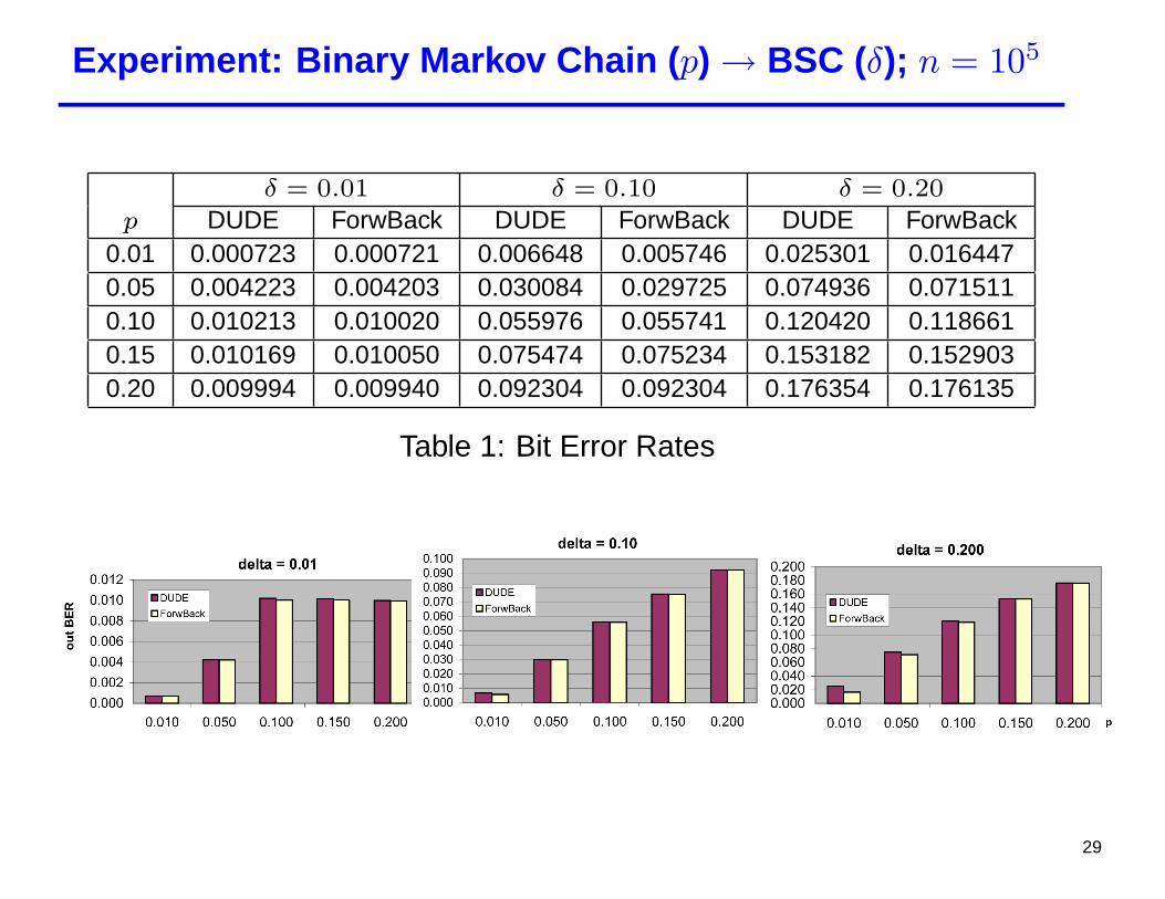
Experiment: Binary Markov Chain ( p) → BSC (δ); n = 105
δ = 0.01 δ = 0.10 δ = 0.20
p DUDE ForwBack DUDE ForwBack DUDE ForwBack0.01 0.000723 0.000721 0.006648 0.005746 0.025301 0.0164470.05 0.004223 0.004203 0.030084 0.029725 0.074936 0.0715110.10 0.010213 0.010020 0.055976 0.055741 0.120420 0.1186610.15 0.010169 0.010050 0.075474 0.075234 0.153182 0.1529030.20 0.009994 0.009940 0.092304 0.092304 0.176354 0.176135
Table 1: Bit Error Rates
29
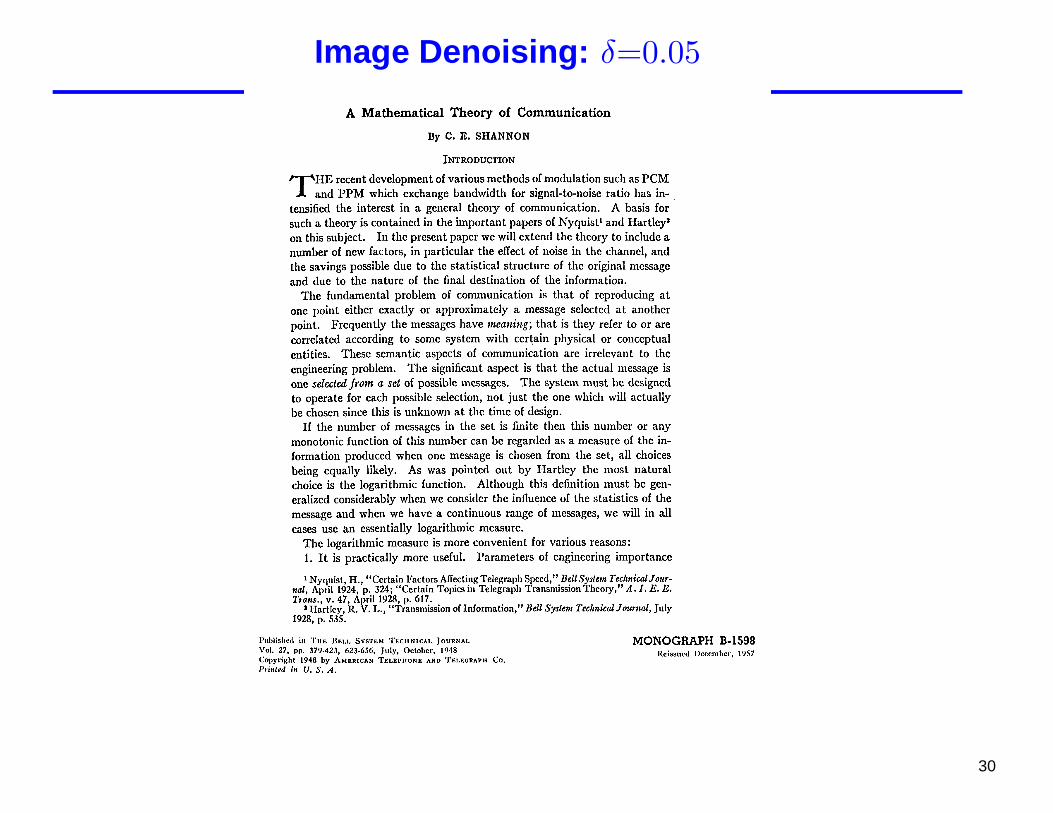
Image Denoising: δ=0.05
30

Image Denoising: δ=0.02
31

Comparison with known algorithms
Channel parameter δ
Image Scheme 0.01 0.02 0.05 0.10Shannon DUDE 0.00096 0.0018 0.0041 0.00911800×2160
median 0.00483 0.0057 0.0082 0.0141morpho. 0.00270 0.0039 0.0081 0.0161
Einstein DUDE 0.0035 0.0075 0.0181 0.0391896×1160
median 0.156 0.158 0.164 0.180morpho. 0.149 0.151 0.163 0.193
32
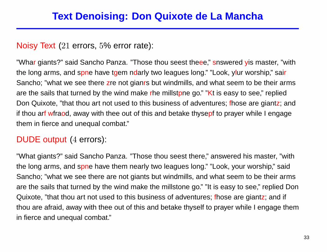
Text Denoising: Don Quixote de La Mancha
Noisy Text (21 errors, 5% error rate):
”Whar giants?” said Sancho Panza. ”Those thou seest theee,” snswered yis master, ”withthe long arms, and spne have tgem ndarly two leagues long.” ”Look, ylur worship,” sairSancho; ”what we see there zre not gianrs but windmills, and what seem to be their armsare the sails that turned by the wind make rhe millstpne go.” ”Kt is easy to see,” repliedDon Quixote, ”that thou art not used to this business of adventures; fhose are giantz; andif thou arf wfraod, away with thee out of this and betake thysepf to prayer while I engagethem in fierce and unequal combat.”
DUDE output (4 errors):
”What giants?” said Sancho Panza. ”Those thou seest there,” answered his master, ”withthe long arms, and spne have them nearly two leagues long.” ”Look, your worship,” saidSancho; ”what we see there are not giants but windmills, and what seem to be their armsare the sails that turned by the wind make the millstone go.” ”It is easy to see,” replied DonQuixote, ”that thou art not used to this business of adventures; fhose are giantz; and ifthou are afraid, away with thee out of this and betake thyself to prayer while I engage themin fierce and unequal combat.”
33
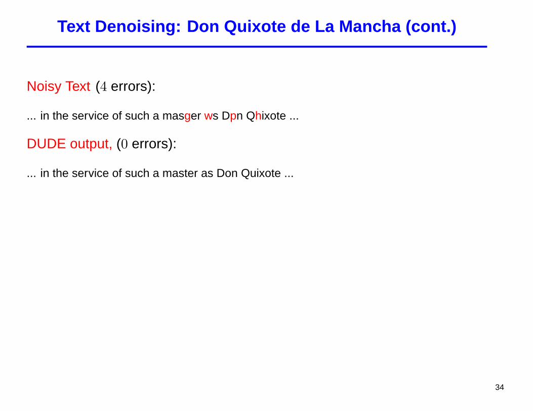
Text Denoising: Don Quixote de La Mancha (cont.)
Noisy Text (4 errors):
... in the service of such a masger ws Dpn Qhixote ...
DUDE output, (0 errors):
... in the service of such a master as Don Quixote ...
34

Measure of Performance
[Normalized cumulative loss] of the denoiser Xn when the observedsequence is zn ∈ An and the underlying clean sequence is xn ∈ An :
LXn(xn, zn) =1n
n∑i=1
Λ(xi, xi),
wherexi = Xn(zn)[i]
We denote the DUDE byXn
DUDE
35
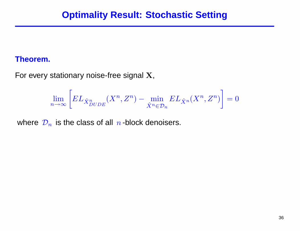
Optimality Result: Stochastic Setting
Theorem.
For every stationary noise-free signal X,
limn→∞
[ELXn
DUDE(Xn, Zn)− min
Xn∈Dn
ELXn(Xn, Zn)]
= 0
where Dn is the class of all n -block denoisers.
36

Optimality Result: Semi-Stochastic Setting
Minimum k -sliding-window loss of (xn, zn) :
Dk(xn, zn) = minf :A2k+1→A
1n− 2k
n−k∑i=k+1
Λ(xi, f(zi+ki−k))
Theorem. For all x ∈ A∞
limn→∞
[LXn
DUDE(xn, Zn)−Dkn(x
n, Zn)]
= 0 a.s.
37
Some Further Directions we will Pursue
• Analogue Data
• Performance boosting tweaks for non-asymptotic regime
• Non-stationary data
• Channel Uncertainty
• Channels with Memory
• Sequentiality Constraint
• Applications to data compression and communications
• ...
38

Compression-based denoising
• Intuition and Philosophy
• Tools
Lossy compression preliminaries:� Rate distortion� Rate distortion theory for ergodic processes� Indirect rate distortion theory� Shannon lower bound� Empirical distribution of rate distortion codes� Universal lossy source coding:· Yang-Kieffer codes· Lossy compression via Markov chain Monte Carlo
• Universal denoising via lossy compression
39
Can DUDE accommodate large, even uncountable,alphabets?
• DUDE will perform poorly when alphabet is large
Repeated occurrence of contexts is rareIs problem better viewed in the analogue world ?
• When alphabets are continuousCount statistic approach is inapplicable
40
Extension of “contextless” DUDE to continuous alphabets
Two-pass DUDE-like approach
• Density estimation of the noisy symbol distribution
• Estimate empirical distribution of the underlying clean symbol
• Reconstruct to minimize the estimated conditional loss
41
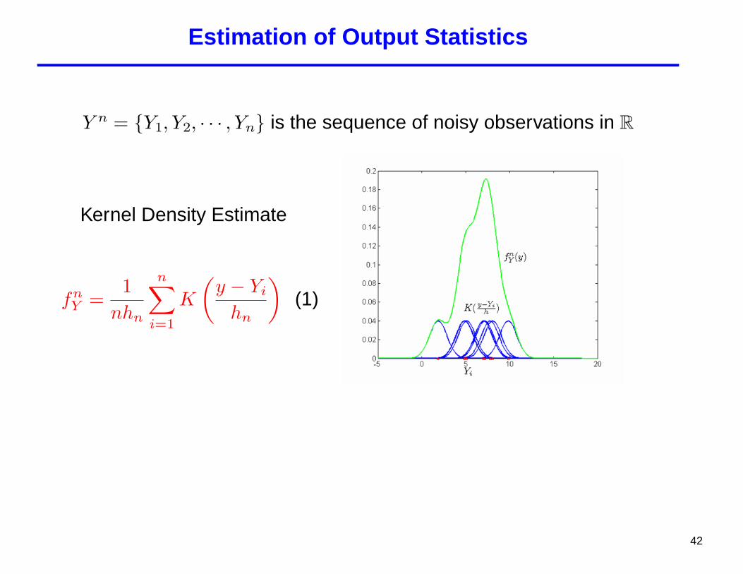
Estimation of Output Statistics
Y n = {Y1, Y2, · · · , Yn} is the sequence of noisy observations in R
Kernel Density Estimate
fnY =
1nhn
n∑i=1
K
(y − Yi
hn
)(1)
42
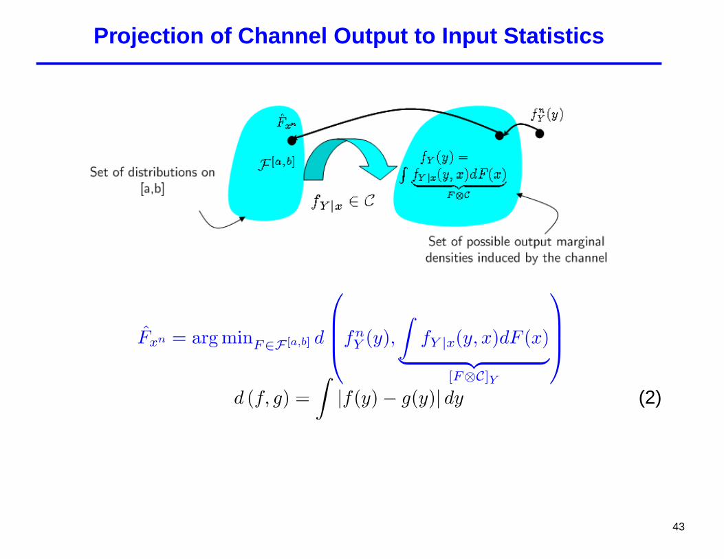
Projection of Channel Output to Input Statistics
Fxn = arg minF∈F [a,b] d
fnY (y),
∫fY |x(y, x)dF (x)︸ ︷︷ ︸
[F⊗C]Y
d (f, g) =
∫|f(y)− g(y)| dy (2)
43

Goodness of Estimation of Clean Signal Statistics
With λ (F,G) denoting Levy distance between F and G
Theorem 1. λ(Fxn, Fxn
)→ 0 a.s. ∀x
44
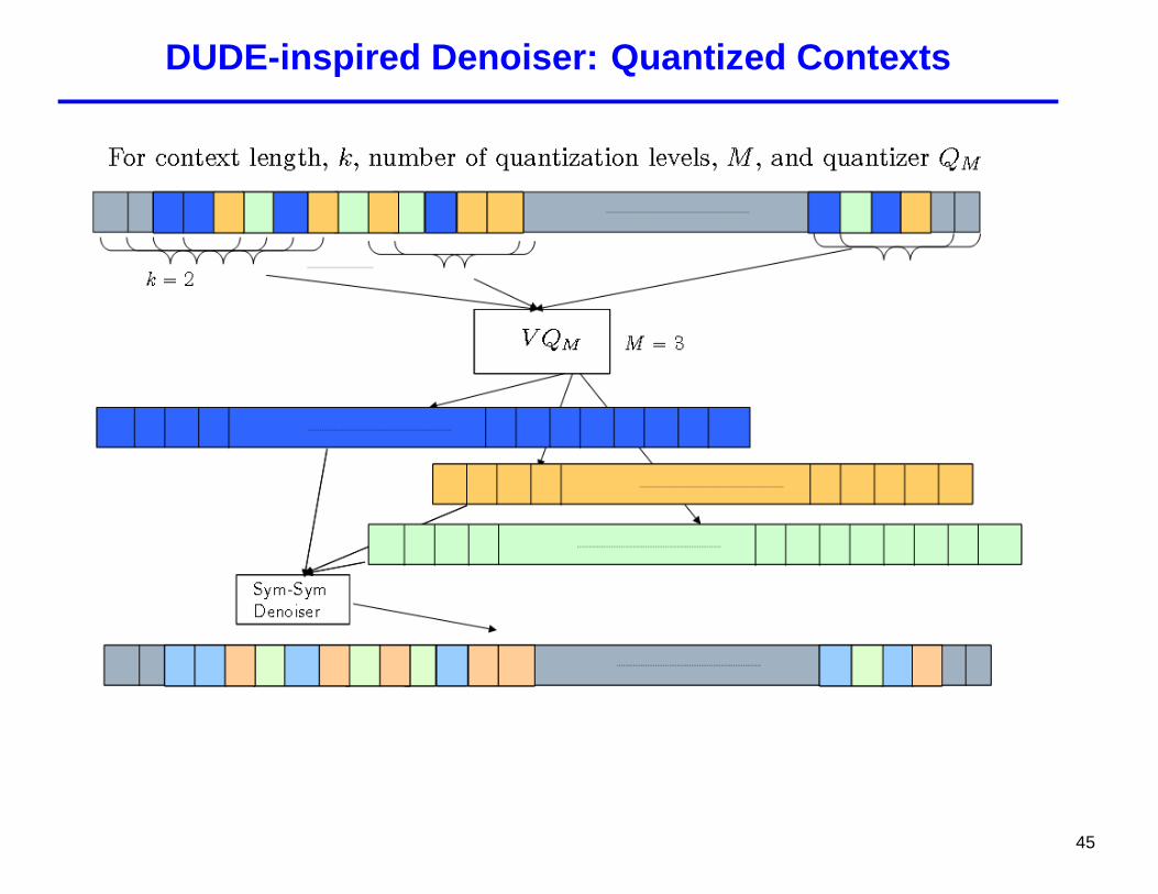
DUDE-inspired Denoiser: Quantized Contexts
45
Computational Complexity
• linear in n
• logarithmic in M
• independent of k
46
Performance Guarantees
Under benign conditions on the channel:
• Can identify the right rate for increase of:
Quantization resolution (with an asymptotically fine partition)Context lengths
• Performance guarantees analogous to those of DUDE in both
semi-stochastic settingstochastic setting
47

Another Approach for Analogue World
Via kernel techniques for vector density estimation
48

Experimental Results
Original Image Image corrupted by AWGN, σ = 20
49
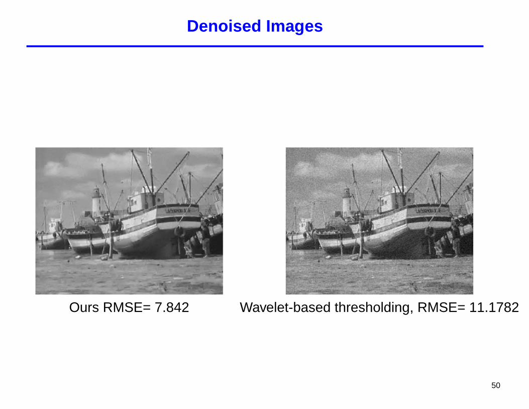
Denoised Images
Ours RMSE= 7.842 Wavelet-based thresholding, RMSE= 11.1782
50

Multiplicative Noise Example
Corrupted by Multiplicative Noise,N (1, 0.2)
51

Denoised Images
Denoised Using BLS-GSM Denoised Using the Proposed Scheme
52
Back to Discrete World: Performance Boosts
• Dynamic contexts
• Context aggregation (inspired by scheme from analogue world)
• Iterated DUDE
53

Performance Boost Example I:DUDE with Context Aggregation
Given
• Distance Function: d(c, c)
• Weight Function: w(c, c)
Outline of CA DUDE Algorithm:
1. Compute count vectors (same as DUDE)
2. Aggregate the counts for similar contexts: for each context c,
• Step 1: Find A = {c | d(c, c) ≤ D}
• Step 2: Compute new context count, mc =∑c∈A
w(c, c)m(c)
3. Denoising decision made based on new context count, mc
54
DUDE with Context Aggregation
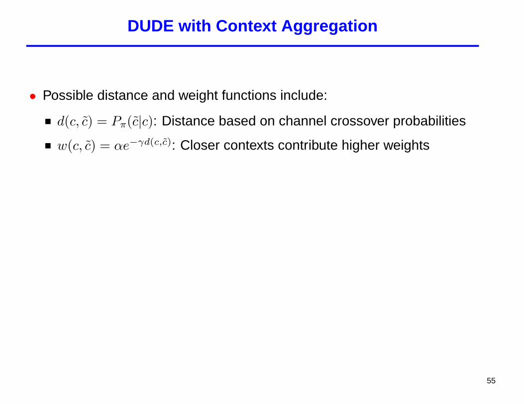
• Possible distance and weight functions include:
d(c, c) = Pπ(c|c): Distance based on channel crossover probabilities
w(c, c) = αe−γd(c,c): Closer contexts contribute higher weights
55
DUDE with Context Aggregation
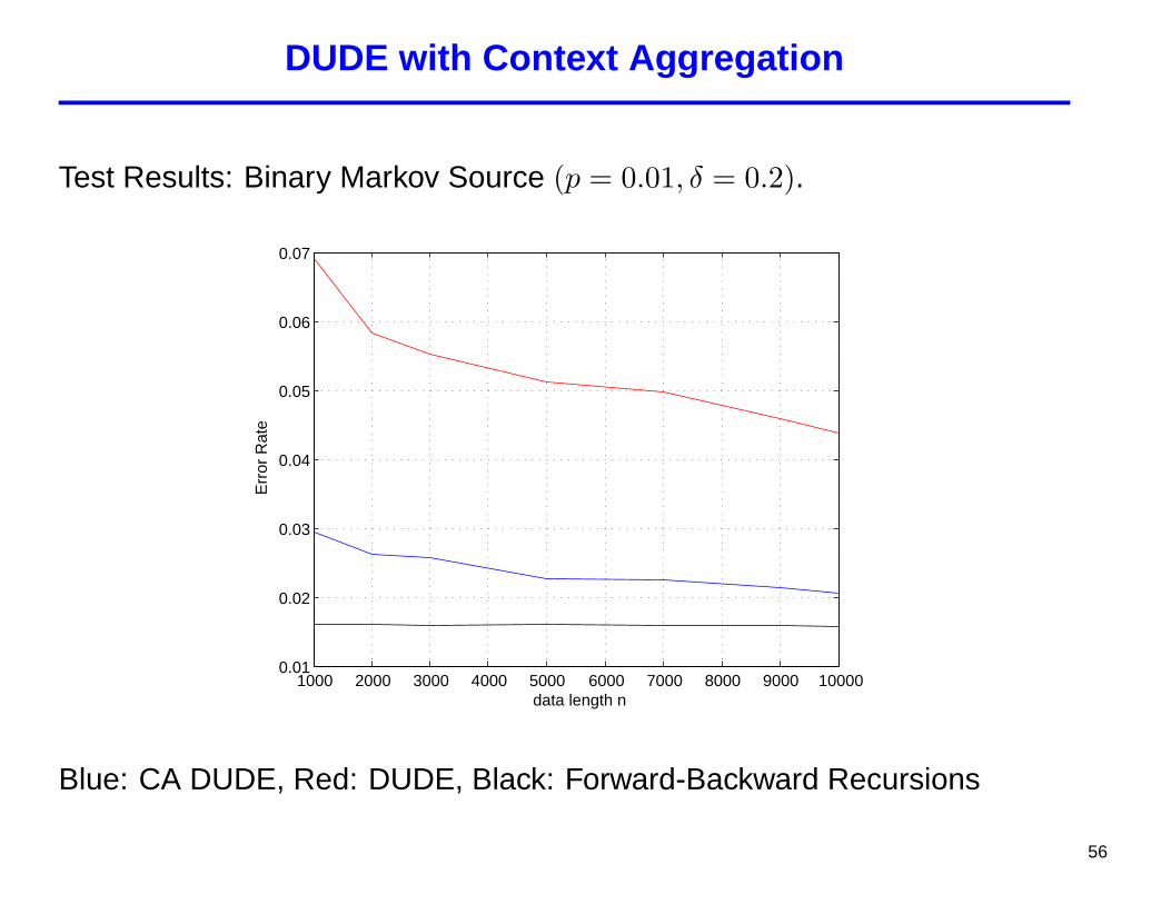
Test Results: Binary Markov Source (p = 0.01, δ = 0.2).
1000 2000 3000 4000 5000 6000 7000 8000 9000 100000.01
0.02
0.03
0.04
0.05
0.06
0.07
data length n
Err
or R
ate
Blue: CA DUDE, Red: DUDE, Black: Forward-Backward Recursions
56

DUDE with Context Aggregation
DUDE: Performance degrades when k is too large
k = 3 (Error rate: 0.0597)
100 200 300 400 500
100
200
300
400
500
k = 4 (Error rate: 0.0839)
100 200 300 400 500
100
200
300
400
500
k = 5 (Error rate: 0.1312)
100 200 300 400 500
100
200
300
400
500
k = 6 (Error rate: 0.1687)
100 200 300 400 500
100
200
300
400
500
57

DUDE with Context Aggregation
Test Results: Bi-Level image corrupted with BSC δ = 0.2
Original Image
100 200 300 400 500
100
200
300
400
500
Noisy Image (Error rate: 0.2)
100 200 300 400 500
100
200
300
400
500
CA DUDE k = 5 (Error rate: 0.051)
100 200 300 400 500
100
200
300
400
500
DUDE k = 3 (Error rate: 0.0597)
100 200 300 400 500
100
200
300
400
500
58

Performance Boost Example II:Iterated DUDE
Possible approaches (in increasing order of sophistication):
• Empirically find the transition matrix H from zn to xn (previousreconstruction), and employ DUDE with Π ·HSimplistic but surprisingly effective:
Table 2: Trial 1 for sequence length of 103, δ = 0.2, (k = 5)iteration 0 1 2 3 error rate
# of errors left 198 34 26 25 0.025Forward-Backward 0.019
Table 3: Trial 1 for sequence length of 104, δ = 0.2, (k = 5)iteration 0 1 2 3 error rate
# of errors left 2003 213 141 136 0.0136Forward-Backward 0.0125
59
Performance Boost Example II:Iterated DUDE (cont.)
• Compute new effective channel at each iteration, and employ DUDE
• Same as previous approach, taking channel memory into account [see“Channels with Memory” below]
60

Perf. boost Ex. III: Accommodating Non-Stationarity
Consider following simplistic motivating example:
• “switching” binary symmetric Markov chain corrupted by BSC (n = 106)
0 1
p
p
1 − p1 − p
δ = 0.1
suppose p = p1 = 0.01 → p = p2 = 0.2 at t∗ = 5× 10⁵ (midpoint)
0 1 2 3 4 5 60.4
0.5
0.6
0.7
0.8
0.9
1
k
Bit
erro
r ra
te/δ
Bit error rate plot for DUDE
DUDEBayes
61

ShifTing Discrete Universal Denoiser (STUD) - 1D data
• can we learn the switch of the source based only on the noisyobservation?
if so, can we do it efficiently?
• reference class: class of k-th order denoisers that allow at most m shifts
3
zn :
{sk} :1 4 7
• Dk,m(xn, zn) : best performance among Snk,m (≤ Dk(xn, zn))
62

STUD - Performance Guarantees
• direct (semi-stochastic setting):when m = o(n), for all x,
limn→∞
[LXn,k,m
STUD(xn, Zn)−Dk,m(xn, Zn)
]= 0 a.s.
• direct (stochastic setting):when m = o(n), achieves optimum performance for any piecewisestationary X
• converse:if m = Θ(n), no denoiser can achieve above
63

Two-pass algorithm
• first pass : forward recursion - update Mt (dynamic programming)
Mt(i, j) = �(zt, j) + min {Mt−1(i, j), min1≤k≤|S| Mt−1(i− 1, k)}
Mt−1 Mt
min
} �(zt, j)+ii
j j
min
• second pass : backward recursion - extract S and denoise
linear complexity in both n and m
64

Example - 1D data (revisited)
• can STUD achieve the optimal BER ?
0 1 2 3 4 5 60.4
0.5
0.6
0.7
0.8
0.9
1
k
Bit
erro
r ra
te/δ
Bit error rate plot for (k,m)−S−DUDE
m=0 (DUDE)m=1Bayes
• m is another “design parameter” for devising a discrete denoiser
65

Extension to 2D data
• what about 2D data?
we need to learn the best segmentation of data1D : disjoint intervals ⇔ 2D : ?
66
STUD - 2D data
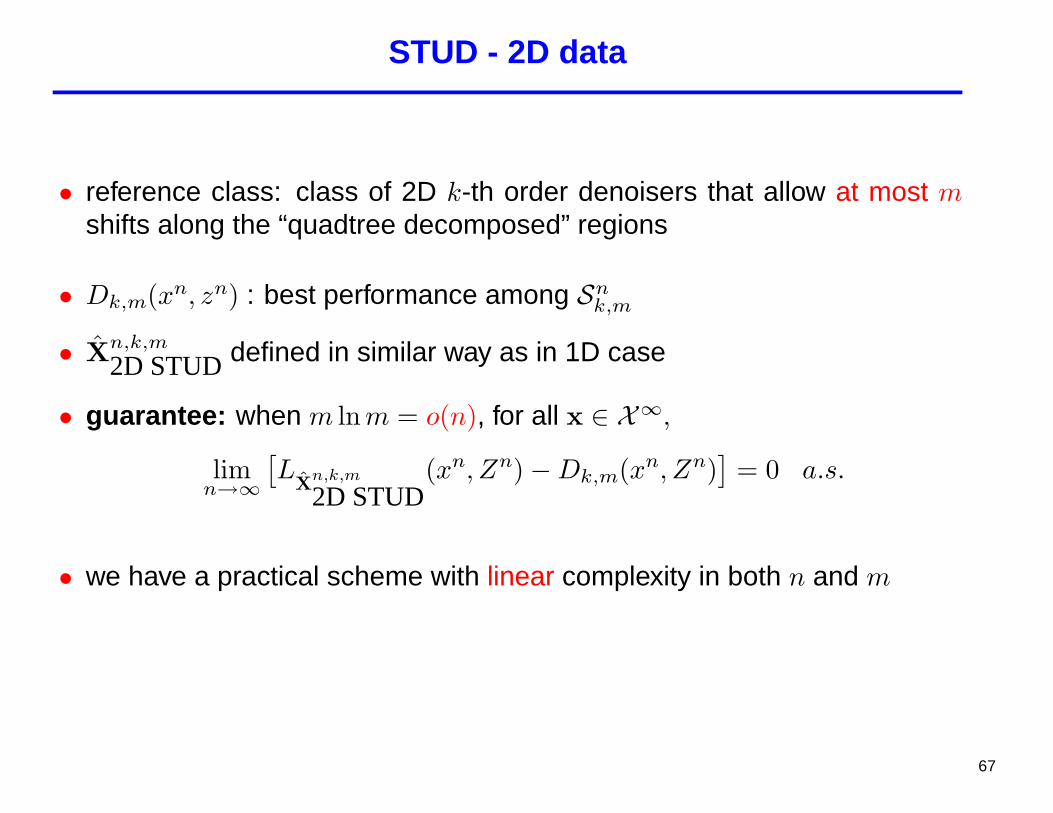
• reference class: class of 2D k-th order denoisers that allow at most mshifts along the “quadtree decomposed” regions
• Dk,m(xn, zn) : best performance among Snk,m
• Xn,k,m
2D STUDdefined in similar way as in 1D case
• guarantee: when m lnm = o(n), for all x ∈ X∞,
limn→∞
[LXn,k,m
2D STUD(xn, Zn)−Dk,m(xn, Zn)
]= 0 a.s.
• we have a practical scheme with linear complexity in both n and m
67
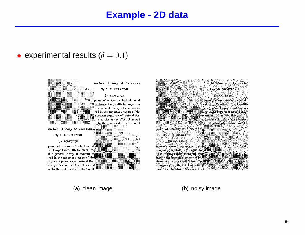
Example - 2D data
• experimental results (δ = 0.1)
(a) clean image (b) noisy image
68

Example - 2D data (cont’d)
• experimental results (δ = 0.1)
1 2 3 4 5 6 70.055
0.06
0.065
0.07
0.075
0.08
k
BE
R
BER plot for Einstein−Shannon block image (d=0.1)
2D Quadtree S−DUDE2D DUDE
69
Channel Uncertainty
Question: In the case of channel uncertainty is there still hope to find adenoiser with the theoretical performance guarantees of the DUDE?
70
Channel Uncertainty
Question: In the case of channel uncertainty is there still hope to find adenoiser with the theoretical performance guarantees of the DUDE?
Answer: Unfortunately not
71

Channel Uncertainty
Approaches that are fruitful in practice:
• DUDE with a “knob”
• DUDE with a channel estimate
• DUDE-like scheme with a channel-independent rule
72

Channels with Memory
• “Single-letter” nature of the DUDE is lost
• Can devise denoisers with performance guarantees analogous to thoseof DUDE
• Case of “additive” noise yields a graceful solution
73
The Sequential LZ-DUDE
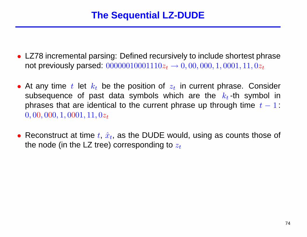
• LZ78 incremental parsing: Defined recursively to include shortest phrasenot previously parsed: 00000010001110zt → 0, 00, 000, 1, 0001, 11, 0zt
• At any time t let kt be the position of zt in current phrase. Considersubsequence of past data symbols which are the kt -th symbol inphrases that are identical to the current phrase up through time t − 1 :0, 00, 000, 1, 0001, 11, 0zt
• Reconstruct at time t, xt, as the DUDE would, using as counts those ofthe node (in the LZ tree) corresponding to zt
74

The Sequential LZ-DUDE: Performance Guarantees
• Performance guarantees analogous to those of DUDE in:
semi-stochastic setting� reference class not only of Markov but of Finite-State filtersstochastic setting
• Fundamental limit different (worse) than for non-sequential case
• Unlike LZ-based predictor, LZ-DUDE does not need to randomize
75

Filtering (causal estimation) ⇔ Prediction ⇔ Compression
We will derive, make mathematically precise, and exploit the followingrelationships:
• Filtering ⇔ Prediction ⇔ Lossless compression
⇓
• Universal compression ⇔ universal predictor ⇒ universal filter
⇓
• LZ compression ⇒ LZ predictor ⇒ LZ-DUDE
76

Application Example: Wyner-Ziv Problem
UnknownSource
DMC
Encoder
Decoder/Denoiser
i(xn) ∈ {1, . . . , 2nR}
xn
xn
zn xn
77

Wyner-Ziv DUDE
Encoder
UnknownSource
DMC Decoder/Denoiser
xn x
n
yn
zn
• Encoding: among yn s.t. LZ(yn) ≤ nR, describe yn most conducive to“DUDE with S.I.” decoder
• Decoding: “DUDE with S.I.”, with yn as a side information sequence
78

Wyner-Ziv DUDE: Main Theoretical Result
• For a source X define:
DX(R) = inf{D : (R,D) is achievable}
Theorem: For any R ≥ 0, and any stationary ergodic source X,
limn→∞
E[distortion (Xn, Reconstruction using Wyner-Ziv DUDE)] = DX(R)
79

Example: Binary Image + WZ-DUDE
Original BSC(0.15)-corrupted version
80

Example: Binary Image + WZ-DUDE (cont.)
Left : Lossy JPEG coding of original image: R = 0.22 b.p.p., BER = 0.0556
Center : DUDE output: BER = 0.0635
Right : WZ-DUDE output: R = 0.22 b.p.p., BER = 0.0407
81

DUDE for Error Correction
Transmitted codeword
Received signalPreprocessed signal
using DUDE
Correct decoding radius
82

So why take this course ?
• Intellectual + practical value of the specific problems considered
• An excuse to learn other topics in information theory
• Opportunity to acquire some tools and see how they are applied
• Learn IT approach to universality
83

Excuse to learn other topics in IT
Beyond our “target” topics, we will pick up:
• State estimation in HMPs and the Forward-Backward scheme
• R-D theory for ergodic sources
• Shannon Lower Bound
• Empirical distribution of good codes
• Indirect R-D
• Ziv-Lempel compression
• Universal prediction
• Compound sequential decision problem
• R-D with decoder side information (Wyner-Ziv problem)
• Systematic channel coding
84

Opportunity to learn some tools and how they are applied
• Martingales
• Concentration Inequalities
• Dynamic Programming
• Markov Chain Monte Carlo
• Density Estimation Techniques
85
Learn IT approach to Universality
Typical IT way of viewing problems:
• Characterization of fundamental limits
• Existence of universal schemes ?
• Universality
Stochastic settingIndividual sequence setting
• Low complexity, practicality, cuteness and grace of schemes
We’ll see this structure for denoising, lossy compression, losslesscompression, prediction, filtering, Wyner-Ziv coding, . . .
Can then apply to your own problems
86