Getting started with tables

Hazel Inskip (hmi@mrc.soton.ac.uk)

Georgia Ntani (gn@mrc.soton.ac.uk)

Leo Westbury (lw@mrc.soton.ac.uk)

Chiara Di Gravio (cdg@mrc.soton.ac.uk)

Stefania D’Angelo (sd@mrc.soton.ac.uk)

Camille Parsons (cp@mrc.soton.ac.uk)

Janis Baird (jb@mrc.soton.ac.uk)

MRC Lifecourse Epidemiology Unit,

University of Southampton

Southampton General Hospital

Southampton

SO16 6YD

Corresponding author: Hazel Inskip, email: hmi@mrc.soton.ac.uk

1

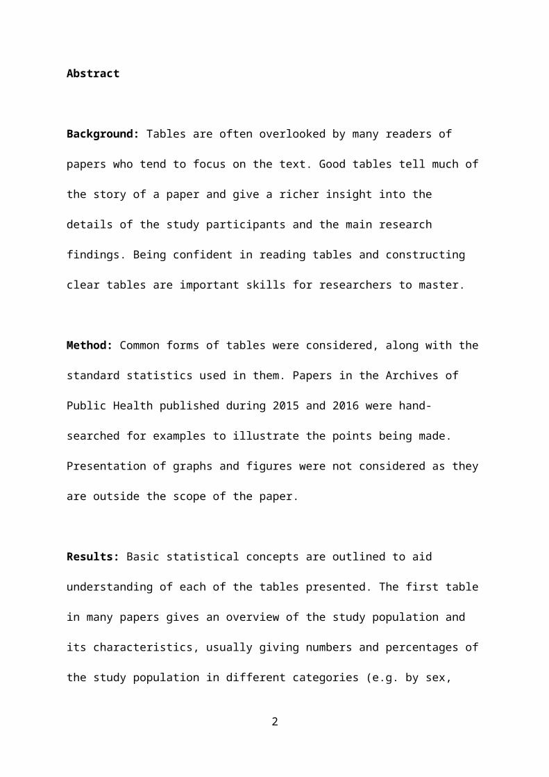
Abstract

Background: Tables are often overlooked by many readers of papers who tend to

focus on the text. Good tables tell much of the story of a paper and give a richer

insight into the details of the study participants and the main research findings. Being

confident in reading tables and constructing clear tables are important skills for

researchers to master.

Method: Common forms of tables were considered, along with the standard

statistics used in them. Papers in the Archives of Public Health published during

2015 and 2016 were hand-searched for examples to illustrate the points being made.

Presentation of graphs and figures were not considered as they are outside the

scope of the paper.

Results: Basic statistical concepts are outlined to aid understanding of each of the

tables presented. The first table in many papers gives an overview of the study

population and its characteristics, usually giving numbers and percentages of the

study population in different categories (e.g. by sex, educational attainment, smoking

status) and summaries of measured characteristics (continuous variables) of the

participants (e.g. age, height, body mass index). Tables giving the results of the

analyses follow; these often include summaries of characteristics in different groups

of participants, as well as relationships between the outcome under study and the

exposure of interest. For continuous outcome data, results are often expressed as

differences between means, or regression or correlation coefficients. Ratio/relative

measures (e.g. relative risks, odds ratios) are usually used for binary outcome

2

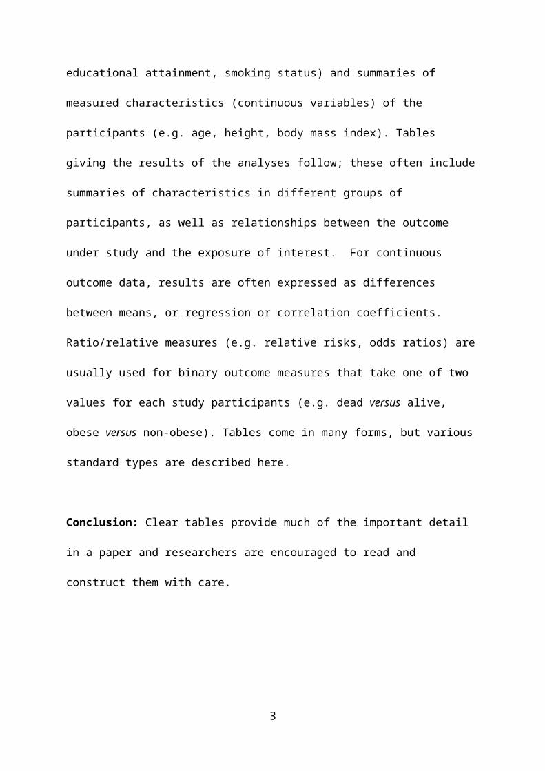
measures that take one of two values for each study participants (e.g. dead versus

alive, obese versus non-obese). Tables come in many forms, but various standard

types are described here.

Conclusion: Clear tables provide much of the important detail in a paper and

researchers are encouraged to read and construct them with care.

Keywords: Tables, variables, characteristics, categories, mean, standard deviation,

median, inter-quartile range, regression coefficients, correlation coefficients, ratios,

relative measures.

3

Introduction

Tables are an important component of any research paper. Yet, anecdotally, many

people say that they find tables difficult to understand so focus only on the text when

reading a paper. However, tables provide a much richer sense of a study population

and the results than can be described in the text. The tables and text complement

each other in that the text outlines the main findings, while the detail is contained in

the tables; the text should refer to each table at the appropriate place(s) in the paper.

We aim to give some insights into reading tables for those who find them

challenging, and to assist those preparing tables in deciding what they need to put

into them. Producing clear, informative tables increases the likelihood of papers

being published and read. Good graphs and figures can often provide a more

accessible presentation of study findings than tables. They can add to the

understanding of the findings considerably, but they can rarely contain as much

detail as a table. Choosing when to present a graph or figure and when to present a

table needs careful consideration but this article focuses only on the presentation of

tables.

We provide a general description of tables and statistics commonly used when

presenting data, followed by specific examples. No two papers will present the tables

in the same way, so we can only give some general insights. The statistical

approaches are described briefly but cannot be explained fully; the reader is referred

to various books on the topic.[1-6]

Presentation of tables

4

The title (or legend) of a table should enable the reader to understand its content, so

a clear, concise description of the contents of the table is required. The specific

details needed for the title will vary according to the type of table. For example, titles

for tables of characteristics should give details of the study population being

summarised and indicate whether separate columns are presented for particular

characteristics, such as sex. For tables of main findings, the title should include the

details of the type of statistics presented or the analytical method. Ideally the table

heading should enable the table to be examined and understood without reference to

the rest of the article, and so information on study, time and place needs to be

included. Footnotes may be required to amplify particular points, but should be kept

to a minimum. Often they will be used to explain abbreviations or symbols used in

the table or to list confounding factors for which adjustment has been made in the

analysis.

Clear heading for rows and columns are also required and the format of the table

needs careful consideration, not least in regard to the appropriateness and number

of rows and columns included within the table. Generally it is better to present tables

with more rows than columns; it is usually easier to read down a table than across it,

and page sizes currently in use are longer than they are wide. Very large tables can

be hard to absorb and make the reader’s work more onerous, but can be useful for

those who require extra detail. Getting the balance right needs care.

Types of tables

Many research articles present a summary of the characteristics of the study

population in the first table. The purpose of these tables is to provide information on

5

the key characteristics of the study participants, and allow the reader to assess the

generalisability of the findings. Typically, age and sex will be presented along with

various characteristics pertinent to the study in question, for example smoking

prevalence, socio-economic position, educational attainment, height, and body mass

index. A single summary column may be presented or perhaps more than one

column split according to major characteristics such as sex (i.e. separate columns for

males and females) or, for trials, the intervention and control groups.

Subsequent tables generally present details of the associations identified in the main

analyses. Sometimes these include results that are unadjusted or ‘crude’ (i.e. don’t

take account of other variables that might influence the association) often followed

by results from adjusted models taking account of other factors.

Other types of tables occur in some papers. For example, systematic review papers

contain tables giving the inclusion and exclusion criteria for the review as well as

tables that summarise the characteristics and results of each study included in the

review; such tables can be extremely large if the review covers many studies.

Qualitative studies often provide tables describing the characteristics of the study

participants in a more narrative format than is used for quantitative studies. This

paper however, focuses on tables that present numerical data.

Statistics commonly presented in tables

The main summary statistics provided within a table depend on the type of outcome

under investigation in the study. If the variable is continuous (i.e. can take any

numerical value, between a minimum and a maximum, such as blood pressure,

height, birth weight), then means and standard deviations (SD) tend to be given

6

when the distribution is symmetrical, and particularly when it follows the classical bell

shaped curve known as a Normal or Gaussian distribution (see Figure 1A). The

mean is the usual arithmetic average and the SD is an indication of the spread of the

values. Roughly speaking, the SD is about a quarter of the difference between the

largest and the smallest value excluding 5% of values at the extreme ends. So, if the

mean is 100 and the SD is 20 we would expect 95% of the values in our data to be

between about 60 (i.e. 100–2x20) and 140 (100+2x40).

The median and inter-quartile range (IQR) are usually provided when the data are

not symmetrical as in Figure 1B, which gives an example of data that are skewed,

such that if the values are plotted in a histogram there are many values at one end of

the distribution but fewer at the other end.[7] If all the values of the variable were

listed in order, the median would be the middle value and the IQR would be the

values a quarter and three-quarters of the way through the list. Sometimes the lower

value of the IQR is labelled Q1 (quartile 1), the median is Q2, and the upper value is

Q3. For categorical variables, frequencies and percentages are used.

Common statistics for associations between continuous outcomes include

differences in means, regression coefficients and correlation coefficients. For these

statistics, values of zero indicate no association between the exposure and outcome

of interest. A correlation coefficient of 0 indicates no association, while a value of 1

or -1 would indicate perfect positive or negative correlation; values outside the range

-1 to 1 are not possible. Regression coefficients can take any positive or negative

value depending on the units of measurement of the exposure and outcome.

7

For binary outcome measures that only take two possible values (e.g. diseased

versus not, dead versus alive, obese versus not obese) the results are commonly

presented in the form of relative measures. These include any measure with the

word ‘relative’ or ‘ratio’ in their name, such as odds ratios, relative risks, prevalence

ratios, incidence rate ratios and hazard ratios. All are interpreted in much the same

way: values above 1 indicate an elevated risk of the outcome associated with the

exposure under study, whereas below 1 implies a protective effect. No association

between the outcome and exposure is apparent if the ratio is 1.

Typically in results tables, 95% confidence intervals (95% CIs) and/or p-values will

be presented. A 95% CI around a result indicates that, in the absence of bias, there

is a 95% probability that the interval includes the true value of the result in the wider

population from which the study participants were drawn. It also gives an indication

of how precisely the study team has been able to estimate the result (whether it is a

regression coefficient, a ratio/relative measure or any of the summary measures

mentioned above). The wider the 95% CI, the less precise is our estimate of the

result. Wide 95% CIs tend to arise from small studies and hence the drive for larger

studies to give greater precision and certainty about the findings.

If a 95% CI around a result for a continuous variable (difference in means,

regression or correlation coefficient) includes 0 then it is unlikely that there is a real

association between exposure and outcome whereas, for a binary outcome, a real

association is unlikely if the 95% CI around a relative measure, such as a hazard or

odds ratio, includes 1.

8

The p-value is the probability that the finding we have observed could have occurred

by chance, and therefore there is no identifiable association between the exposure of

interest and the outcome measure in the wider population. If the p-value is very

small, then we are more convinced that we have found an association that is not

explained by chance (though it may be due to bias or confounding in our study).

Traditionally a p-value of less than 0.05 (sometimes expressed as 5%) has been

considered as ‘statistically significant’ but this is an arbitrary value and the smaller

the p-value the less likely the result is simply due to chance.[8]

Frequently, data within tables are presented with 95% CIs but without p-values or

vice versa. If the 95% CI includes 0 (for a continuous outcome measure) or 1 (for a

binary outcome), then generally the p-value will be greater than 0.05, whereas if it

does not include 0 or 1 respectively, then the p-value will be less than 0.05.[9]

Generally, 95% CIs are more informative than p-values; providing both may affect

the readability of a table and so preference should generally be given to 95% CIs.

Sometimes, rather than giving exact p-values, they are indicated by symbols that are

explained in a footnote; commonly one star (*) indicates p<0.05, two stars (**)

indicates p<0.01.

Results in tables can only be interpreted if the units of measurement are clearly

given. For example, mean or median age could be in days, weeks, months or years

if infants and children are being considered, and 365, 52, 12 or 1 for a mean age of 1

year could all be presented, as long the unit of measurement is provided. Standard

deviations should be quoted in the same units as the mean to which they refer.

9

Relative measures, such as odds ratios, and correlation coefficients do not have

units of measurement, but for regression coefficients the unit of measurement of the

outcome variable is required, and also of the exposure variable if it is continuous.

Examples

The examples are all drawn from recent articles in Archives of Public Health. They

were chosen to represent a variety of types of tables seen in research publications.

Tables of characteristics

The table of characteristics in Figure 2 is from a study assessing knowledge and

practice in relation to tuberculosis control among in Ethiopian health workers.[10]

The authors have presented the characteristics of the health workers who

participated in the study. Summary statistics are based on categories of the

characteristics, so numbers (frequencies) in each category and the percentages of

the total study population within each category are presented for each characteristic.

From this, the reader can see that:

the study population is quite young, as only around 10% are more than 40 years

old;

the majority are female;

more than half are nurses;

about half were educated to degree level or above.

The table of characteristics in Figure 3, is from a study of the relationship between

distorted body image and lifestyle in adolescents in Japan.[11] Here the presentation

is split into separate columns for boys and girls. The first four characteristics are

10

continuous variables, not split into categories but, instead, presented as means, with

the SDs given in brackets. The three characteristics in the lower part of the table are

categorical variables and, similar to Figure 1, the frequency/numbers and

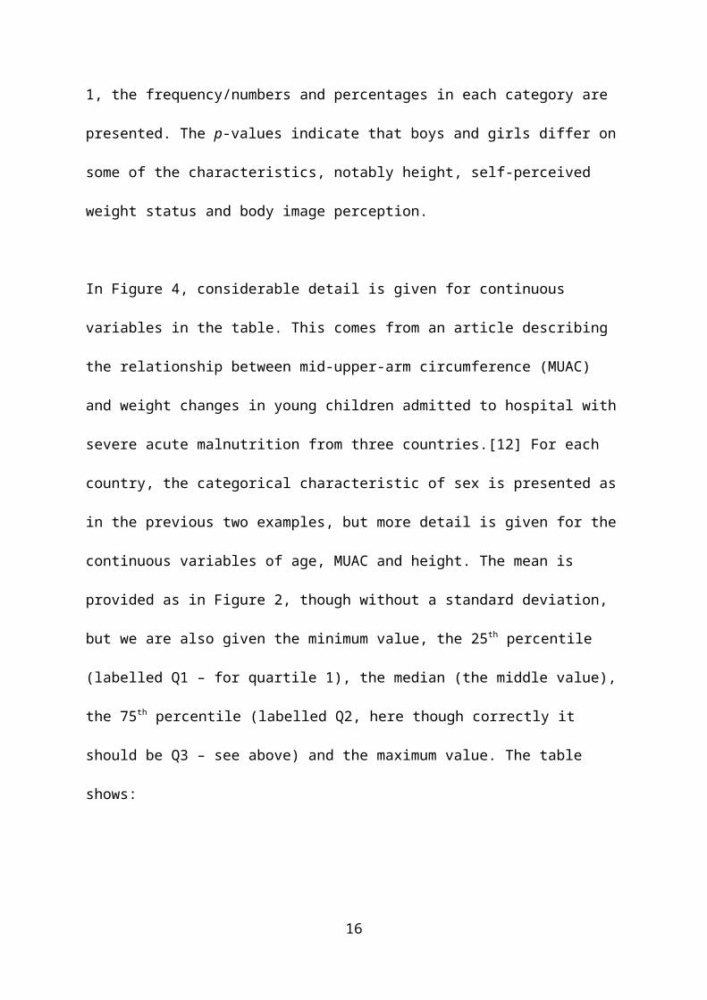
percentages in each category are presented. The p-values indicate that boys and

girls differ on some of the characteristics, notably height, self-perceived weight status

and body image perception.

In Figure 4, considerable detail is given for continuous variables in the table. This

comes from an article describing the relationship between mid-upper-arm

circumference (MUAC) and weight changes in young children admitted to hospital

with severe acute malnutrition from three countries.[12] For each country, the

categorical characteristic of sex is presented as in the previous two examples, but

more detail is given for the continuous variables of age, MUAC and height. The

mean is provided as in Figure 2, though without a standard deviation, but we are

also given the minimum value, the 25th percentile (labelled Q1 – for quartile 1), the

median (the middle value), the 75th percentile (labelled Q2, here though correctly it

should be Q3 – see above) and the maximum value. The table shows:

Ethiopian children in this study were older and taller than those from the other

two countries but their MUAC measurements tended to be smaller;

in Bangladesh, disproportionally more females than males were admitted for

treatment compared with the other two countries.

It is unusual to present as much detail on continuous characteristics as is given in

Figure 4. Usually, for each characteristic, either (a) mean and SD or (b) median and

IQR would be given, but not both.

11

Tables of results – summary findings

Many results tables are simple summaries and look similar to tables presenting

characteristics, as described above. Sometimes the initial table of characteristics

includes some basic comparisons that indicate the main results of the study. Figure

5 shows part of a large table of characteristics for a study of risk factors for acute

lower respiratory infections (ALRI) among young children in Rwanda.[13] In addition

to presenting the numbers of children in each category of a variety of characteristics,

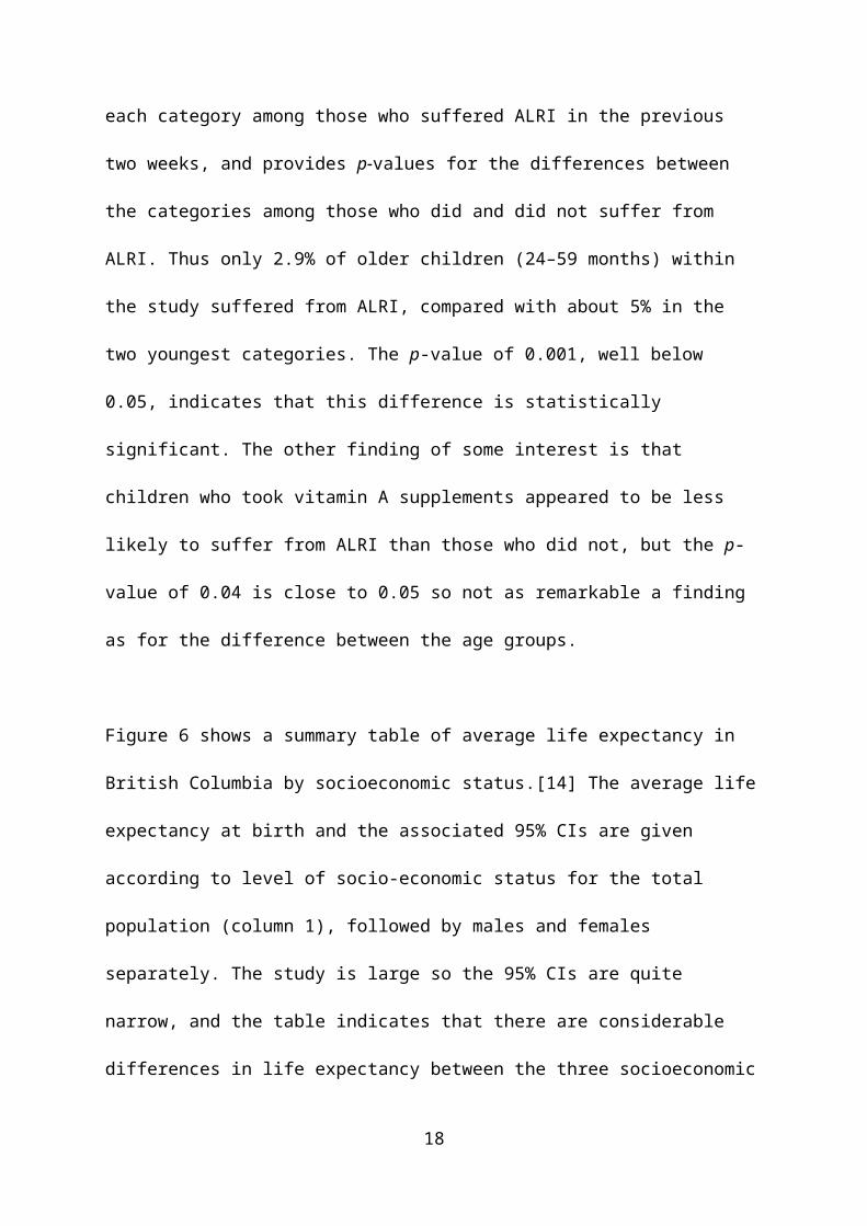
it also shows the percentage in each category among those who suffered ALRI in the

previous two weeks, and provides p-values for the differences between the

categories among those who did and did not suffer from ALRI. Thus only 2.9% of

older children (24–59 months) within the study suffered from ALRI, compared with

about 5% in the two youngest categories. The p-value of 0.001, well below 0.05,

indicates that this difference is statistically significant. The other finding of some

interest is that children who took vitamin A supplements appeared to be less likely to

suffer from ALRI than those who did not, but the p-value of 0.04 is close to 0.05 so

not as remarkable a finding as for the difference between the age groups.

Figure 6 shows a summary table of average life expectancy in British Columbia by

socioeconomic status.[14] The average life expectancy at birth and the associated

95% CIs are given according to level of socio-economic status for the total

population (column 1), followed by males and females separately. The study is large

so the 95% CIs are quite narrow, and the table indicates that there are considerable

differences in life expectancy between the three socioeconomic groups, with the

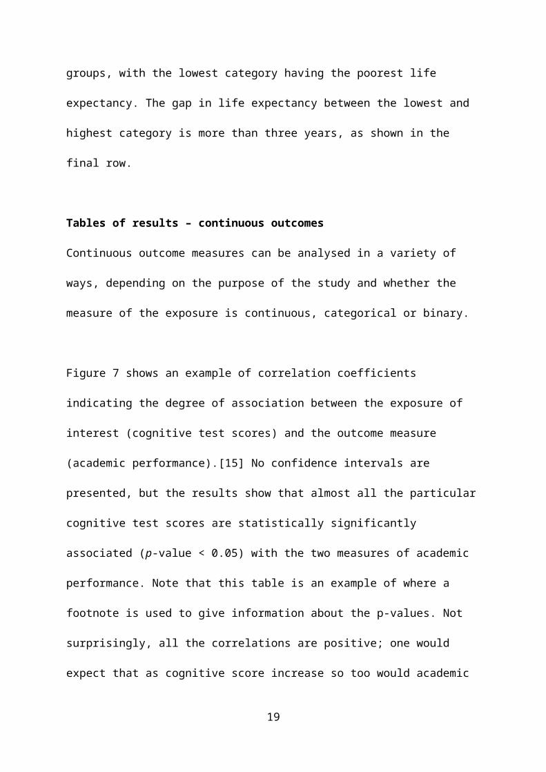
lowest category having the poorest life expectancy. The gap in life expectancy

12

between the lowest and highest category is more than three years, as shown in the

final row.

Tables of results – continuous outcomes

Continuous outcome measures can be analysed in a variety of ways, depending on

the purpose of the study and whether the measure of the exposure is continuous,

categorical or binary.

Figure 7 shows an example of correlation coefficients indicating the degree of

association between the exposure of interest (cognitive test scores) and the outcome

measure (academic performance).[15] No confidence intervals are presented, but

the results show that almost all the particular cognitive test scores are statistically

significantly associated (p-value < 0.05) with the two measures of academic

performance. Note that this table is an example of where a footnote is used to give

information about the p-values. Not surprisingly, all the correlations are positive; one

would expect that as cognitive score increase so too would academic performance.

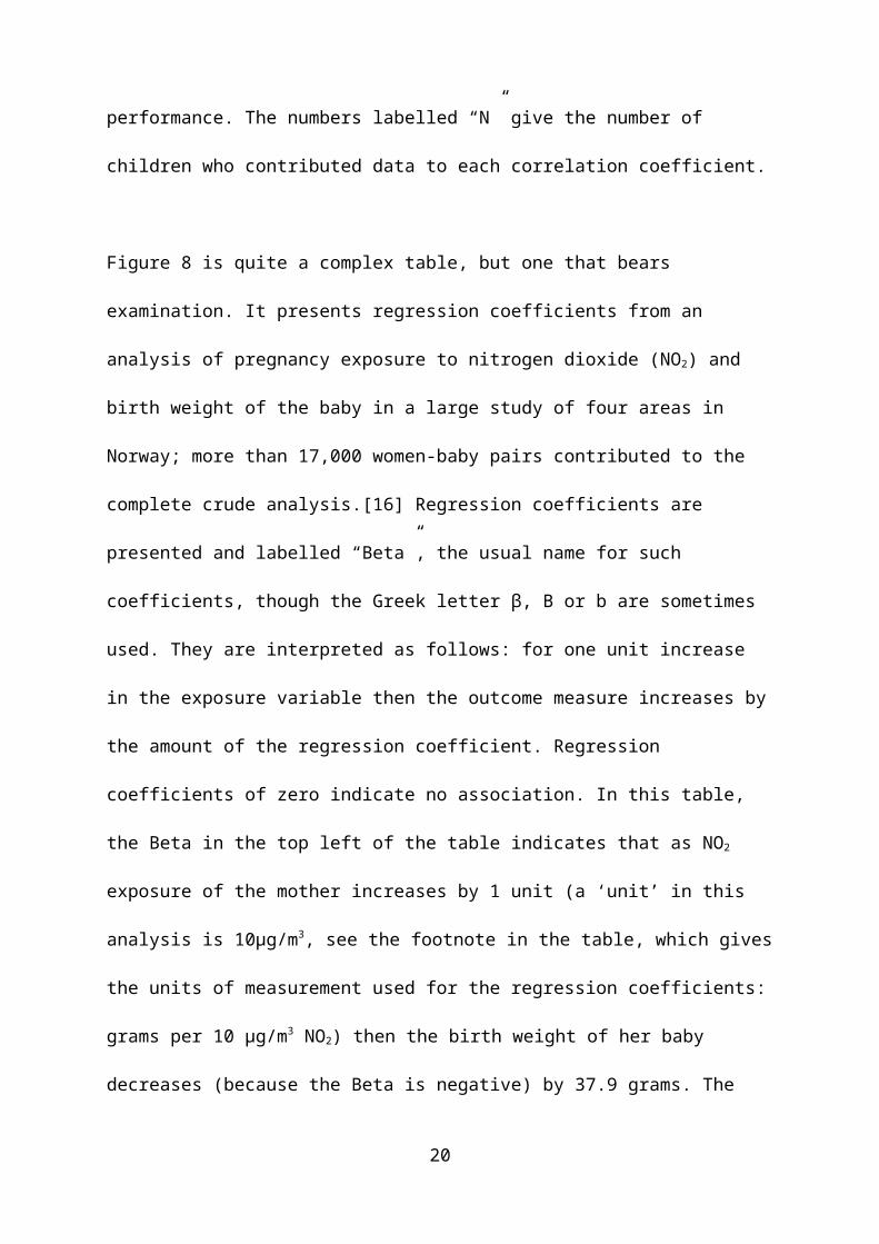
The numbers labelled “N” give the number of children who contributed data to each

correlation coefficient.

Figure 8 is quite a complex table, but one that bears examination. It presents

regression coefficients from an analysis of pregnancy exposure to nitrogen dioxide

(NO2) and birth weight of the baby in a large study of four areas in Norway; more

than 17,000 women-baby pairs contributed to the complete crude analysis.[16]

Regression coefficients are presented and labelled “Beta”, the usual name for such

coefficients, though the Greek letter β, B or b are sometimes used. They are

13

interpreted as follows: for one unit increase in the exposure variable then the

outcome measure increases by the amount of the regression coefficient. Regression

coefficients of zero indicate no association. In this table, the Beta in the top left of the

table indicates that as NO2 exposure of the mother increases by 1 unit (a ‘unit’ in this

analysis is 10µg/m3, see the footnote in the table, which gives the units of

measurement used for the regression coefficients: grams per 10 µg/m3 NO2) then the

birth weight of her baby decreases (because the Beta is negative) by 37.9 grams.

The 95% CI does not include zero and the p-value is small (<0.001) implying that the

association is not due solely to chance.

However, reading across the columns of the table gives a different story. The

successive sets of columns include adjustment for increasing numbers of factors that

might affect the association. While model 1 still indicates a negative association

between NO2 and birth weight that is highly significant (p < 0.001), models 2 and 3

do not. Inclusion of adjustment for parity or area and maternal weight have reduced

the association such that the Betas have shrunk in magnitude to be closer to 0, with

95% CIs including 0 and p-values >0.05.

The table has multiple rows, with each one providing information on a different

subset of the data, so the numbers in the analyses are all smaller than in the first

row. The second row restricts the analysis to women who did not move address

during pregnancy, an important consideration in estimating NO2 exposure from home

addresses. The third row restricts the analysis to those whose gestational age was

based on the last menstrual period. These second two rows present ‘sensitivity

analyses’, performed to check that the results were not due to potential biases

14

resulting from women moving house or having uncertain gestational ages. The

remaining rows in the table present stratified analyses, with results given for each

category of various variables of interest, namely geographical area, maternal

smoking, parity, baby’s sex, mother’s educational level and season of birth. Only one

row of this table has a statistically significant result for models 2 and 3, namely

babies born in spring, but this finding is not discussed in the paper. Note the gap in

the table in the model 2 column as it is not possible to adjust for area (one of the

adjustment factors in model 2) when the analysis is being presented for each area

separately.

Tables of results – binary outcomes

Figure 9 presents results from a study assessing whether children’s eating styles are

associated with having a waist-hip ratio greater or equal to 0.5 (the latter being the

outcome variable expressed in binary form – ≥0.5 versus <0.5).[17] Results for boys

and girls are presented separately, along with the number of children in each of the

eating style categories. The main results are presented as crude and adjusted odds

ratios (ORs). The adjusted ORs take account of age, exercise, skipping breakfast

and having a snack after dinner, all of these being variables thought to affect the

association between eating style and waist-hip ratio. Looking at the crude OR

column, the value of 2.04 in the first row indicates that, among boys, those who

report eating quickly have around twice the odds of having a high waist-hip ratio than

those who do not eat quickly (not eating quickly is the baseline category, with an

odds ratio given as 1.00). The 95% CI for the crude OR for eating quickly is 1.31 to

3.18. This interval does not include 1, indicating that the elevated OR for eating

quickly is unlikely to be a chance finding and that there is a 95% probability that the

15

range of 1.31 to 3.18 includes the true OR. The p-value is 0.002, considerably

smaller than 0.05, indicates that this finding is ‘statistically significant’. The other ORs

can be considered in the same way, but note that, for both boys and girls, the ORs

for eating until full are greater than 1 but their 95% CIs include 1 and the p-values

are considerably greater than 0.05, so not ‘statistically significant’, indicating chance

findings.

The final columns present the ORs after adjustment for various additional factors,

along with their 95% CIs and p-values. The ORs given here differ little from the crude

ORs in the table, indicating that the adjustment has not had much effect, so the

conclusions from examining the crude ORs are unaltered. It thus appears that eating

quickly is strongly associated with a greater waist-hip ratio, but that eating until full is

not.

Conclusion

Summary tables of characteristics describe the study population and set the study in

context. The main findings can be presented in different ways and choice of

presentation is determined by the nature of the variables under study. Scrutiny of

tables allows the reader to acquire much information about the study and a richer

insight than if the text only is examined. Constructing clear tables that communicate

the nature of the study population and the key results is important in the preparation

of papers; good tables can assist the reader enormously as well as increasing the

chance of the paper being published.

Abbreviations

16

ALRI Acute lower respiratory infections

CI Confidence interval

MUAC Mid-upper-arm circumference

IQR Inter-quartile range

NO2 Nitrogen dioxide

OR Odds ratio

Q1 Quartile 1 (25th percentile)

Q2 Quartile 2 (50th percentile = median)

Q3 Quartile 3 (75th percentile)

SD Standard deviation

Declarations

Not applicable

Ethics Approval and Consent to Participate

Not applicable

Consent for publication

Not applicable

Availability of data and materials

Data sharing is not applicable to this article as no datasets were generated or

analysed during the current study

Competing interests

17

The authors declare that they have no competing interests.

Funding

The work was funded by the UK Medical Research Council which funds the work of

the MRC Lifecourse Epidemiology Unit where the authors work. The funding body

had no role in the design and conduct of the work, or in the writing the manuscript.

Authors’ contributions

HI conceived the idea for the paper in discussion with JB. HI wrote the first draft and

all other authors commented on successive versions and contributed ideas to

improve content, clarity and flow of the paper. All authors read and approved the

final manuscript.

Acknowledgement

Not applicable

18

Reference List

1. Peacock J, Peacock P: Oxford Handbook of Medical Statistics. Oxford: Oxford University Press; 2010.

2. Bland M: An Introduction to Medical Statistics. 4th edn. Oxford: Oxford University Press; 2015.

3. Kirkwood BR, Sterne JAC: Essential Medical Statistics. 2nd edn. Oxford: Wiley-Blackwell; 2003.

4. Altman DG: Practical statistics for medical research. London: Chapman & Hall; 1991.

5. Everitt BS, Palmer C: Encyclopaedic Companion to Medical Statistics. 2nd edn. Chichester: Wiley; 2010.

6. Armitage P, Berry G, Matthews JNS: Statistical Methods in Medical Research. 4th edn. Oxford: Wiley; 2001.

7. Inskip HM, Godfrey KM, Robinson SM, Law CM, Barker DJ, Cooper C, SWS Study Group: Cohort profile: The Southampton Women's Survey. Int J Epidemiol 2006, 35:42-48.

8. Sterne JA, Davey Smith G: Sifting the evidence-what's wrong with significance tests? BMJ 2001, 322:226-231.

9. What are confidence intervals and p-values? [http://www.medicine.ox.ac.uk/bandolier/painres/download/whatis/what_are_conf_inter.pdf]

10. Demissie Gizaw G, Aderaw Alemu Z, Kibret KT: Assessment of knowledge and practice of health workers towards tuberculosis infection control and associated factors in public health facilities of Addis Ababa, Ethiopia: A cross-sectional study. Archives of Public Health 2015, 73:1-9.

11. Shirasawa T, Ochiai H, Nanri H, Nishimura R, Ohtsu T, Hoshino H, Tajima N, Kokaze A: The relationship between distorted body image and lifestyle among Japanese adolescents: a population-based study. Archives of Public Health 2015, 73:1-7.

12. Binns P, Dale N, Hoq M, Banda C, Myatt M: Relationship between mid upper arm circumference and weight changes in children aged 6–59 months. Archives of Public Health 2015, 73:1-10.

13. Harerimana J-M, Nyirazinyoye L, Thomson DR, Ntaganira J: Social, economic and environmental risk factors for acute lower respiratory infections among children under five years of age in Rwanda. Archives of Public Health 2016, 74:1-7.

14. Zhang LR, Rasali D: Life expectancy ranking of Canadians among the populations in selected OECD countries and its disparities among British Columbians. Archives of Public Health 2015, 73:1-10.

15. Haile D, Nigatu D, Gashaw K, Demelash H: Height for age z score and cognitive function are associated with Academic performance among school children aged 8–11 years old. Archives of Public Health 2016, 74:1-7.

16. Panasevich S, Håberg SE, Aamodt G, London SJ, Stigum H, Nystad W, Nafstad P: Association between pregnancy exposure to air pollution and birth weight in selected areas of Norway. Archives of Public Health 2016, 74:1-9.

19

17. Ochiai H, Shirasawa T, Nanri H, Nishimura R, Matoba M, Hoshino H, Kokaze A: Eating quickly is associated with waist-to-height ratio among Japanese adolescents: a cross-sectional survey. Archives of Public Health 2016, 74:1-7.

20

Legends for figures

Figure 1. Distribution of heights and weights of young women from the Southampton Women’s Survey [7]. Figure 4A shows the height distribution, which is symmetrical and generally follows a standard normal distribution, while Figure 4B shows weight, which is skewed to the right.

Figure 2. Table of study population characteristics from a paper on the assessment of knowledge and practice in relation to tuberculosis control in health workers in Ethiopia.[10]

Figure 3. Table of study population characteristics from a paper on the relationship between distorted body image and lifestyle in adolescents in Japan.[11]

Figure 4. Table of study population characteristics from a paper describing the relationship between mid-upper-arm circumference (MUAC) and weight changes in young children.[12]

Figure 5. Part of a table of basic results from a study of risk factors for acute lower respiratory infections (ALRI) among young children in Rwanda.[13]

Figure 6. Summary table of average life expectancy in British Columbia by socioeconomic status.[14]

Figure 7. Correlation coefficients from a study assessing the association between cognitive function and academic performance in Ethiopia. [15]

Figure 8. Table of regression coefficients for the relationship between exposure to NO2 in pregnancy and birth weight. [16]

Figure 9. Results table from a study assessing whether children’s eating styles are associated with having a waist-hip ratio ≥0.5 or not.[17]

21