Thesis for the Master degree in Mathematics. Department of Mathematical Sciences, University

of Copenhagen

Speciale for cand.scient graden i matematik. Institut for matematiske fag, Københavns

Universitet

On Almost Commuting Operatorsand Matrices

Advisor/Vejleder: Mikael Rørdam

Peter Bech Møller Sørensen

30. april 2012

Abstract

This master thesis is about almost commuting matrices, and a Brown-Douglas-Fillmore Theorem. The main results are:

In the part about almost commuting matrices it is shown that almostcommuting self-adjoint matrices can be uniformly approximated by exactlycommuting self-adjoint matrices (Lin’s theorem), and some non-trivial coun-terexamples are given about almost commuting unitaries, and almost com-muting pairs consisting of a self-adjoint and a normal matrix. Other simplerrelated questions are also examined.

In the part about the Brown-Douglas-Fillmore theorem it is shown thatan essentially normal operator is a compact perturbation of a normal oper-ator if and only if it has trivial index function.

In this connection a short introduction to Fredholm operators is alsogiven.

Resume: Dette speciale handler om næsten kommuterende matricer,og et Brown-Douglas-Fillmore Theorem. Hovedresultaterne er:

I den del der handler om næsten kommuterende matricer vises det atnækommuterende selvadjungerede matricer kan approximeres uniformt medexact kommuterende selvadjungerede matrices (Lins sætning), og nogle ikke-trivielle modeksempler gives vedrørende næsten kommuterende unitære ma-tricer, og næsten kommuterende par bestaende af en selvadjungeret og nor-mal matrix. Andre enklerer relaterede spørgsmal undersøges ogsa.

I den del der handler om Brown-Douglas-Fillmore teoremet vises detat en essentielt normal operator er en kompakt perturbation a en normaloperator hvis og kun hvis den har triviel index funktion.

Contents

1 Introduction 2Some remarks on notation, approximation, lifting problems,

corner algebras, and polar decomposition . . . . . . . 3

2 Some Questions, and Some Answers 72.1 Index Theory and a Brown-Douglas Fillmore Theorem . . . . 7

Fredholm Operators and Index . . . . . . . . . . . . . . . . . 7A Brown-Douglas-Fillmore Theorem . . . . . . . . . . . . . . 12

2.2 Almost Commuting Matrices . . . . . . . . . . . . . . . . . . 14Projections . . . . . . . . . . . . . . . . . . . . . . . . . . . . 15Self-adjoints . . . . . . . . . . . . . . . . . . . . . . . . . . . . 16Unitaries and Normals . . . . . . . . . . . . . . . . . . . . . . 18

2.3 Quasidiagonal Operators and The Weyl-von Neummann-BergTheorem . . . . . . . . . . . . . . . . . . . . . . . . . . . . . . 19Quasidiagonal Operators . . . . . . . . . . . . . . . . . . . . . 19Proof of the Weyl-von Neumann-Berg Theorem using Lin’s

Theorem . . . . . . . . . . . . . . . . . . . . . . . . . 22

3 Lin’s Theorem 233.1 Proof that the set of normal elements with finite spectrum is

dense in the set of normal elements in M/A . . . . . . . . . . 243.2 Constructing Almost Commuting Matrices . . . . . . . . . . . 27

4 Two Counterexamples 324.1 A Topological Obstruction . . . . . . . . . . . . . . . . . . . . 324.2 Three Almost Commuting Matrices . . . . . . . . . . . . . . . 34

5 A BDF-Theorem 425.1 Proof of Theorem 5.4 . . . . . . . . . . . . . . . . . . . . . . . 43

1

Chapter 1

Introduction

The topics which will be discussed in this master thesis are some naturaltopics one might consider when recalling the following classical theoremabout operators on a finite dimensional Hilbert space.

Theorem 1.1. Let N be a normal operator on a finite dimensional Hilbertspace. Then there exists an orthonormal basis where N is diagonal.

This theorem, which says that two self-adjoint operators on a finite di-mensional Hilbert space can be simultaneously diagonalized, has many directgeneralizations, to several operators and compact operators on an infinte-dimensional Hilbert space (For instance any family of mutually commutingnormal compact operators can be simultaneously diagonalized).

The main topic of of this text can loosely be described as an attemptto answer the following (vague) question: If an operator is not normal, butin some sense close to being normal, is it then close to a normal operator?Of course we have to specify what we mean by ‘close to being normal’, and‘close to a normal operator’. We will think of this in primarily two differentways:

1. Loosely speaking we will call an operator whose self-commutant hassmall norm ‘almost normal’, and we will say two operators are close if thenorm of their difference is small. First we will ask whether operators (mostlyon a finite dimensional Hilbert space), which are almost normal are close tonormal operators. We will formulate this more precisely in section 2.2. Thissection is really about when two almost commuting operators of some species(say self-adjoint) are close to commuting operators of the same species. Themain result here is Lin’s Theorem, which will be proved in chapter 3. Wewill also focus on some interesting non-trivial counterexamples in chapter 4.

2. Secondly we will ask when operators with compact self-commutant,are compact perturbations of normal operators. Operators with compactself-commutant will be called essentially normal. To answer this preciselywe need the notion of Fredholm index, and the main result is a so-called

2

Brown-Douglas-Fillmore (BDF) theorem. BDF-theory is a theory aboutclassification of essentially normal operators. We will only touch upon oneof the theorems from BDF-theory (however the most famous one). Theprecise statement will be given in 2.1, and the proof will be given in chapter5, and uses Lin’s theorem.

In section 2.3 we will show some elementary things about quasidiago-nal operators, and use Lin’s theorem to give a short proof of the Weyl-vonNeumann-Berg Theorem for one normal operator on a Hilbert space. Thetheorem can be seen as answer to a natural question one can ask in connec-tion with Theorem 1.1: Is a normal operator, which is not necessarily com-pact, diagonalizable, or at least close to being diagonal in some orthonormalbasis?

Some remarks on notation, approximation, lifting problems,corner algebras, and polar decomposition

Let H be a Hilbert Space, B(H), BK(H), and Bf (H) be respectively thebounded, compact, and finite rank operators on H. From now on we willassume, although it is not always necessary, H to be separable .

We will extensively use the theory of C∗-algebras to prove our results. Inparticular in connection with almost commuting matrices we will introducethe following two C∗-algebras. Let (nk) be a sequence of natural numbersand define:

M = (Ak) | Ak ∈Mnk(C) and supk∈N||Ak|| <∞, (1.1)

andA = (Ak) | Ak ∈Mnk(C) and lim

k→∞||Ak|| = 0. (1.2)

With coordinate-wise definitions of addition, multiplication and adjoints Mand A are C∗-algebras. Moreover M is a von Neumann algebra, so we canapply Borel function calculus and stay within it. A is obviously a closedself-adjoint two-sided ideal in M so we can consider the quotient algebraM/A which is also a C∗-algebra. We denote the quotient mapping by π,which is a continuous ∗-homomorphism.

In connection with the BDF-theorem we shall use the Calkin algebra,B(H)/BK(H), which we will denote Q(H). The compact operators in aHilbert space is a self-adjoint two-sided ideal in B(H), so Q(H) is a C∗-algebra (we assume these results to be already established). We again useπ for the canonical homomorphism from B(H) into Q(H) - this should notlead to any confusion although we already used it for M/A, since they willappear in different contexts.

3

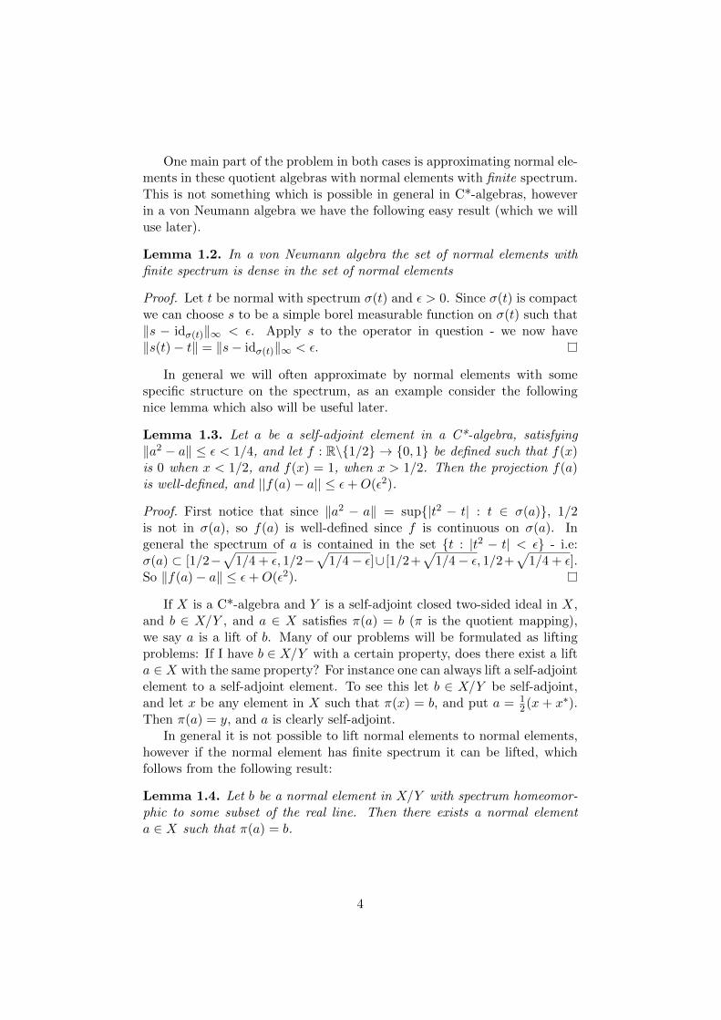
One main part of the problem in both cases is approximating normal ele-ments in these quotient algebras with normal elements with finite spectrum.This is not something which is possible in general in C*-algebras, howeverin a von Neumann algebra we have the following easy result (which we willuse later).

Lemma 1.2. In a von Neumann algebra the set of normal elements withfinite spectrum is dense in the set of normal elements

Proof. Let t be normal with spectrum σ(t) and ε > 0. Since σ(t) is compactwe can choose s to be a simple borel measurable function on σ(t) such that‖s − idσ(t)‖∞ < ε. Apply s to the operator in question - we now have‖s(t)− t‖ = ‖s− idσ(t)‖∞ < ε.

In general we will often approximate by normal elements with somespecific structure on the spectrum, as an example consider the followingnice lemma which also will be useful later.

Lemma 1.3. Let a be a self-adjoint element in a C*-algebra, satisfying‖a2 − a‖ ≤ ε < 1/4, and let f : R\1/2 → 0, 1 be defined such that f(x)is 0 when x < 1/2, and f(x) = 1, when x > 1/2. Then the projection f(a)is well-defined, and ||f(a)− a|| ≤ ε+O(ε2).

Proof. First notice that since ‖a2 − a‖ = sup|t2 − t| : t ∈ σ(a), 1/2is not in σ(a), so f(a) is well-defined since f is continuous on σ(a). Ingeneral the spectrum of a is contained in the set t : |t2 − t| < ε - i.e:σ(a) ⊂ [1/2−

√1/4 + ε, 1/2−

√1/4− ε]∪ [1/2+

√1/4− ε, 1/2+

√1/4 + ε].

So ‖f(a)− a‖ ≤ ε+O(ε2).

If X is a C*-algebra and Y is a self-adjoint closed two-sided ideal in X,and b ∈ X/Y , and a ∈ X satisfies π(a) = b (π is the quotient mapping),we say a is a lift of b. Many of our problems will be formulated as liftingproblems: If I have b ∈ X/Y with a certain property, does there exist a lifta ∈ X with the same property? For instance one can always lift a self-adjointelement to a self-adjoint element. To see this let b ∈ X/Y be self-adjoint,and let x be any element in X such that π(x) = b, and put a = 1

2(x + x∗).Then π(a) = y, and a is clearly self-adjoint.

In general it is not possible to lift normal elements to normal elements,however if the normal element has finite spectrum it can be lifted, whichfollows from the following result:

Lemma 1.4. Let b be a normal element in X/Y with spectrum homeomor-phic to some subset of the real line. Then there exists a normal elementa ∈ X such that π(a) = b.

4

Proof. Let b ∈ X/Y be normal, and let f be a homeomorphism which mapsσ(b) to a subset of the real line. Lift f(b) to a self-adjoint element x ∈ X,as remarked above. Let f be a continuous function from R into C which isidentical to f−1 on σ(f(b)). Put a = f(x) which is normal by continuousfunction calculus, and we have π(a) = π(f(x)) = f(π(x)) = (f f)(b) =b.

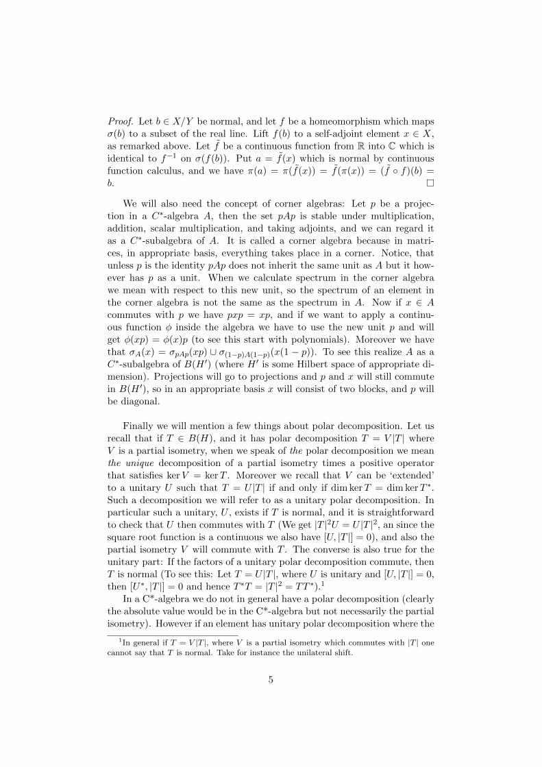
We will also need the concept of corner algebras: Let p be a projec-tion in a C∗-algebra A, then the set pAp is stable under multiplication,addition, scalar multiplication, and taking adjoints, and we can regard itas a C∗-subalgebra of A. It is called a corner algebra because in matri-ces, in appropriate basis, everything takes place in a corner. Notice, thatunless p is the identity pAp does not inherit the same unit as A but it how-ever has p as a unit. When we calculate spectrum in the corner algebrawe mean with respect to this new unit, so the spectrum of an element inthe corner algebra is not the same as the spectrum in A. Now if x ∈ Acommutes with p we have pxp = xp, and if we want to apply a continu-ous function φ inside the algebra we have to use the new unit p and willget φ(xp) = φ(x)p (to see this start with polynomials). Moreover we havethat σA(x) = σpAp(xp) ∪ σ(1−p)A(1−p)(x(1 − p)). To see this realize A as aC∗-subalgebra of B(H ′) (where H ′ is some Hilbert space of appropriate di-mension). Projections will go to projections and p and x will still commutein B(H ′), so in an appropriate basis x will consist of two blocks, and p willbe diagonal.

Finally we will mention a few things about polar decomposition. Let usrecall that if T ∈ B(H), and it has polar decomposition T = V |T | whereV is a partial isometry, when we speak of the polar decomposition we meanthe unique decomposition of a partial isometry times a positive operatorthat satisfies kerV = kerT . Moreover we recall that V can be ‘extended’to a unitary U such that T = U |T | if and only if dim kerT = dim kerT ∗.Such a decomposition we will refer to as a unitary polar decomposition. Inparticular such a unitary, U , exists if T is normal, and it is straightforwardto check that U then commutes with T (We get |T |2U = U |T |2, an since thesquare root function is a continuous we also have [U, |T |] = 0), and also thepartial isometry V will commute with T . The converse is also true for theunitary part: If the factors of a unitary polar decomposition commute, thenT is normal (To see this: Let T = U |T |, where U is unitary and [U, |T |] = 0,then [U∗, |T |] = 0 and hence T ∗T = |T |2 = TT ∗).1

In a C*-algebra we do not in general have a polar decomposition (clearlythe absolute value would be in the C*-algebra but not necessarily the partialisometry). However if an element has unitary polar decomposition where the

1In general if T = V |T |, where V is a partial isometry which commutes with |T | onecannot say that T is normal. Take for instance the unilateral shift.

5

composants commute then the element is indeed normal - the proof is in thesame way as before.

Let us also note that for the adjoint we have a polar decomposition by:

T ∗ = |T |V ∗ = (V ∗V )|T |V ∗ = V ∗(|T |V ∗)

Since |T | is positive TV ∗ = V |T |V ∗ is positive. Moreover ker(TV ∗) =kerV ∗: Clearly kerV ∗ ⊂ ker(TV ∗). To see the other inclusion assume x ∈ker(TV ∗) but not in kerV ∗ to obtain a contradiction. We then have V ∗x ∈kerT = kerV . Hence V ∗x ∈ V ∗(H)⊥, which means V ∗x = 0, since V ∗ ispartial isometry. This establishes the contradiction. From the uniquenessof the polar decomposition we must therefore have |T ∗| = V |T |V ∗, so:

T ∗ = V ∗|T ∗|

Finally by taking adjoints we also have:

T = |T ∗|V.

6

Chapter 2

Some Questions, and SomeAnswers

In this chapter we make a precise formulation of the two main theorems wewant to prove, and consider some related questions.

2.1 Index Theory and a Brown-Douglas FillmoreTheorem

We want to investigate when an essentially normal operator is a compactperturbation of a normal operator. In order to formulate the result we needto introduce the Fredholm index, and prove some fundamental results.

Recall that an operator A is essentially normal if its self-commutant[A,A∗] is compact, or equivalently that π(A) is normal in the Calkin algebra.The essential spectrum of A we define to be the spectrum of π(A) and wedenote it σess(A).

Fredholm Operators and Index

It is worth recalling that kerT ∗ = (T (H))⊥, which we will use constantly inwhat follows.

Definition 2.1. An operator T ∈ B(H) is called a Fredholm operator ifand only if T has closed range, and the kernels of T and T ∗ are both finite-dimensional. The collection of Fredholm operators is denoted by F (H).Moreover for a Fredholm operator T we define its index as the integerdim kerT−dim kerT ∗. For n ∈ Z we let Fn(H) denote the class of Fredholmoperators with index n.

The function which takes each Fredholm operator to its index we willdenote just by index. Moreover, in this connection, we will view Z as agroup with respect to addition, and equip it with the discrete topology.

7

We notice that any invertible operator A is Fredholm, and has index 0,moreover if T ∈ Fn(H) then AT ∈ Fn(H), and T ∗ ∈ F−n(H).

If T is a normal Fredholm operator then the index of T is zero since T ∗

and T have identical kernels (||Tx|| = 0 is equivalent to ||T ∗x|| = 0 becauseT is normal).

Let U+ be the unilateral shift - we see that index Un+ = −n and indexU∗n+ = n, so no Fredholm classes are empty.

To each Fredholm operator T there exists a partial inverse in the follow-ing sense:

Proposition 2.2. Let T ∈ F (H). There exists a unique S ∈ F (H) withkerS = kerT ∗ and kerS∗ = kerT , and such that ST is the projection ontokerT⊥, and TS is the projection onto (kerT ∗)⊥.

Proof. Let T : kerT⊥ → T (H) be equal to the restriction of T . Since T isbijective and T (H) is closed by assumption it has a bounded inverse S. LetS : H → H be the linear extension of S by letting S = 0 on T (H)⊥ = kerT ∗.S has the desired properties.

The following fundamental result is often called Atkinson’s Theorem.

Theorem 2.3. An operator T ∈ B(H) is a Fredholm operator if and onlyπ(T ) is invertible in the Calkin algebra.

Proof. That π(T ) is invertible in the Calkin algebra means that there existsan operator S ∈ B(H) such that both ST − I and TS− I are compact, andwe see that the ‘only if’ part of the proof follows from the existense of apartial inverse which we have already established.

It remains to be shown that if π(T ) is invertible in the Calkin algebrathen T is a Fredholm operator. Since π(T ) is invertible there exists S ∈B(H) such that ST = I + K, and TS = 1 + K ′, where K, and K ′ arecompact operators. We now have:

kerT ⊂ ker(ST ) = ker(1 +K) = eigenvectors of K with eigenvalue -1

Since K ′ is compact it can have at most finite dimension of eigenspaces whichare not associated with eigenvalue 0. Hence kerT has finite dimension.

By using T ∗S∗ = I+K∗, we similarly show that the dimension of kerT ∗

is finite.To see that T (H) is closed it is enough to show that T restricted to

(kerT )⊥ is bounded from below. Assume it is not bounded from below.Then there exists a sequence of unit vectors (xn) ∈ (kerT )⊥ such that‖Txn‖ < 1/n.

Hence Txn → 0.Hence STxn → 0.Hence (1 +K)xn → 0.

8

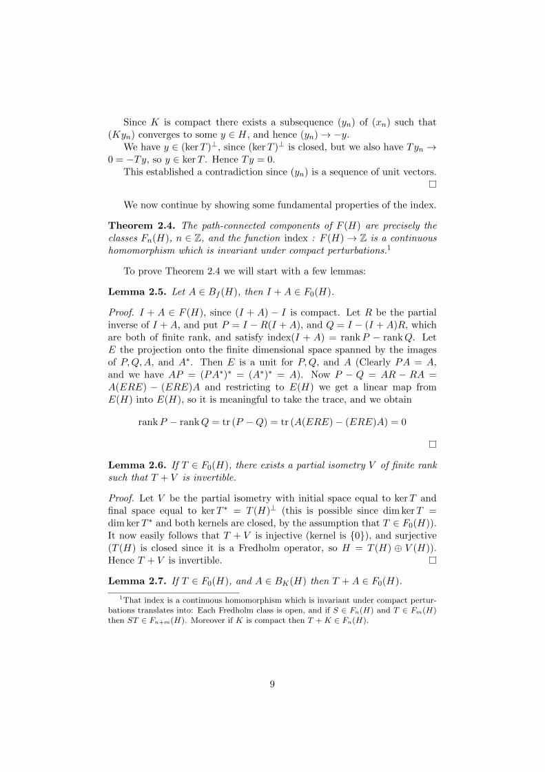
Since K is compact there exists a subsequence (yn) of (xn) such that(Kyn) converges to some y ∈ H, and hence (yn)→ −y.

We have y ∈ (kerT )⊥, since (kerT )⊥ is closed, but we also have Tyn →0 = −Ty, so y ∈ kerT . Hence Ty = 0.

This established a contradiction since (yn) is a sequence of unit vectors.

We now continue by showing some fundamental properties of the index.

Theorem 2.4. The path-connected components of F (H) are precisely theclasses Fn(H), n ∈ Z, and the function index : F (H)→ Z is a continuoushomomorphism which is invariant under compact perturbations.1

To prove Theorem 2.4 we will start with a few lemmas:

Lemma 2.5. Let A ∈ Bf (H), then I +A ∈ F0(H).

Proof. I + A ∈ F (H), since (I + A) − I is compact. Let R be the partialinverse of I +A, and put P = I −R(I +A), and Q = I − (I +A)R, whichare both of finite rank, and satisfy index(I + A) = rankP − rankQ. LetE the projection onto the finite dimensional space spanned by the imagesof P,Q,A, and A∗. Then E is a unit for P,Q, and A (Clearly PA = A,and we have AP = (PA∗)∗ = (A∗)∗ = A). Now P − Q = AR − RA =A(ERE) − (ERE)A and restricting to E(H) we get a linear map fromE(H) into E(H), so it is meaningful to take the trace, and we obtain

rankP − rankQ = tr (P −Q) = tr (A(ERE)− (ERE)A) = 0

Lemma 2.6. If T ∈ F0(H), there exists a partial isometry V of finite ranksuch that T + V is invertible.

Proof. Let V be the partial isometry with initial space equal to kerT andfinal space equal to kerT ∗ = T (H)⊥ (this is possible since dim kerT =dim kerT ∗ and both kernels are closed, by the assumption that T ∈ F0(H)).It now easily follows that T + V is injective (kernel is 0), and surjective(T (H) is closed since it is a Fredholm operator, so H = T (H) ⊕ V (H)).Hence T + V is invertible.

Lemma 2.7. If T ∈ F0(H), and A ∈ BK(H) then T +A ∈ F0(H).

1That index is a continuous homomorphism which is invariant under compact pertur-bations translates into: Each Fredholm class is open, and if S ∈ Fn(H) and T ∈ Fm(H)then ST ∈ Fn+m(H). Moreover if K is compact then T +K ∈ Fn(H).

9

Proof. By Lemma 2.6 Let V be a partial isometry of finite rank such thatT + V is invertible

Since the Bf (H) is dense in BK(H) we can choose a finite rank operatorF such ‖F −A‖ < ‖(T + V )−1‖−1.

Put R = T + V +A− F = (T + V )(I + (T + V )−1(A− F ).We have I+(T+V )−1(A−F ) is invertible since ‖(T+V )−1(A−F )‖ < 1,

and hence R is invertible. We now have:

index(T +A) = index(R(I +R−1(F − V ))) = index(I +R−1(F − V )) = 0,

where we in the second last inequality used that multiplication by an invert-ible operator does not change the Fredholm class, and in the last inequalitywe used that R−1(F − V ) ∈ Bf (H) and Lemma 2.5

We now interlude our search for a proof of 2.4 with proving the followingtheorem for compact operators known as the Fredholm Alternative:

Theorem 2.8. Let A ∈ BK(H), and let λ ∈ σ(A)\0, then λ is an eigen-value for A with finite multiplicity. Moreover λ is an eigenvalue for K∗ withthe same multiplicity.

Proof. Let λ ∈ σ(A)\0, and assume that λ is not an eigenvalue of A withfinite multiplicity (i.e. either an eigenvalue with infinite multiplicity or notan eigenvalue at all). Put T = I − λ−1A. By Lemma 2.7 T ∈ F0(H),since A is compact. Since T is Fredholm kerT is finite-dimensional, andλ therefore cannot be an eigenvalue with infinite multiplicity. Hence λ isnot an eigenvalue, and kerT must be 0. Moreover since T is FredholmT (H) is closed. Hence T (H) = (kerT ∗)⊥, but since T ∈ F0(H) we havekerT ∗ = 0 (since kerT = 0), and hence T (H) = H. So T is invertiblecontradicting λ ∈ σ(A).

The last part about K∗ follows from dim kerT ∗ = dim kerT , and T ∗ =

I − λ−1A∗.

Lemma 2.9. F0(H) is open in B(H).

Proof. Assume the result is not true. Then for some T ∈ F0(H) there existsa sequence (Tn) in B(H) converging to T , where each Tn /∈ F0(H). ByLemma 2.6 there exist a partial isometry V of finite rank such that T + Vis invertible. Since the collection of invertible elements is open in B(H)there exists a positive integer N such that TN + V is invertible, and henceTN + V ∈ F0(H). Since −V is compact TN = (TN + V ) − V ∈ F0(H) byLemma 2.7, contradicting the way (Tn) was constructed.

Before we proceed, we remark the following with respect to direct sums:Let H = H1⊕H2, where H1 and H2 are Hilbert spaces. Let S ∈ F (H1) and

10

let T ∈ F (H2), then index(S ⊕ T ) = index(S) + index(T ).

Proof that compact perturbations do not change index:Let T ∈ Fn(H) for some integer n, and let A ∈ BK(H). We now

have: (T + A) ⊕ T ∗ = T ⊕ T ∗ + A ⊕ 0, and since index(T ⊕ T ∗) = 0 andA ⊕ 0 is compact we have from Lemma 2.7 and index((T + A) ⊕ T ∗) =index(T ⊕ T ∗ + A ⊕ 0) = 0. By Atkinson’s theorem T + A is a Fredholmoperator since A is compact. Hence index(T +A) = n, as desired.

Proof that each Fredholm class is open:Let T ∈ Fn(H). We have T ⊕ T ∗ ∈ F0(H ⊕ H). By Lemma 2.9 there

exists an open neighborhood U of T ⊕T ∗ contained in F0(H⊕H), for whichwe have U ∩ B(H) ⊕ T ∗ ⊂ Fn(H) ⊕ T ∗. This shows U ∩ B(H) ⊕ T ∗ is anopen subset in the induced topology on B(H)⊕T ∗ contained in Fn(H)⊕T ∗,which shows what we want since T was arbitrary.

Proof that index is a homomorphism:Let T, S ∈ F (H). Since S ⊕ S∗ ∈ F0(H ⊕ H) there exists a partial

isometry V such that S ⊕ S∗ + V is invertible, by Proposition 2.6. Now wehave:

index(T ) = index(T ⊕ I) = index((T ⊕ I)(S ⊕ S∗ + V ))

= index(TS ⊕ S∗ + (T ⊕ I)V ) = index(TS ⊕ S∗)= index(TS)− index(S),

where we in the second equality used that multiplying by an invertible op-erator does not change the index, and in the second last equality we usedthe result proved above that compact perturbations do not change the index.

To show that the Fredholm classes are path-connected we need the fol-lowing two results:

Proposition 2.10. In B(H) the collection of unitary operators are path-connected.

Proof. Let U ∈ B(H) be unitary. We will show there exists a continuouspath connecting U to the identity. Let Arg : C\0 → [0; 2π[ be the ar-gument function on the complex plane. This is a bounded borel functioninto the real numbers, and hence A := Arg(U) is selfadjoint. Let now thecontinuous path be defined by t 7→ etiA, for t ∈ [0, 1]. Since A is selfadjointetiA is unitary for all t ∈ [0, 1]. It is straightforward to see that the path iscontinuous.

Proposition 2.11. In B(H) the collection of invertible operators are path-connected.

11

Proof. Let T ∈ B(H) be an invertible operator, with polar decompositionT = UP , where U is unitary and P is strictly positive. By Proposition2.10 there exists a continuous path from [0, 1] 3 t 7→ Ut connecting theidentity to U . Together with the continuous path [0, 1] 3 t 7→ Pt, wherePt = (1− t)I + tP is an invertible positive operator (To see the invertibilitylook at σ(Pt)), the result follows.

Proof that each Fredholm class is path-connected :Assume n ≥ 0 (Since Fn(H)∗ = F−n(H) and the adjoint map is contin-

uous this is without loss of generality).First we notice that a Fredholm operator T with index n, can be con-

nected by a path in Fn(H) to an operator in Fn(H) which kernel has dimen-sion n (and hence is surjective). To see this let V be a partial isometry withinitial space contained in kerT and image equal to kerT ∗ (This is possiblesince n ≥ 0). Define a continuous path by t 7→ T + tV , where t ∈ [0, 1]. Forany t > 0 it is clear that T + tV is surjective and the dimension of its kernelis n.

Secondly we notice that if R, T ∈ Fn(H) and their kernels have equaldimension there exists a continuous path in Fn(H) connecting R to R ∈Fn(H) with same kernel as T . To see this let U be a unitary such thekerRU = kerT , and put R = RU , and let t 7→ Ut be a path of unitaryoperators from I to U (using Proposition 2.10). Now since the the unitariesare invertible t 7→ RUt is a map into Fn(H) since multiplication by aninvertible operator does not change the index.

We thus only have to show that if R, T ∈ Fn(H) are surjective operatorswith identical kernel, then they can be connected by a continuous path. Tosee this consider the restrictions of R and T to the orthogonal complement oftheir kernels. These restrictions are now invertible, and we can use Proposi-tion 2.11 to path-connect the restricted operators with invertible operators.Extending the operators in this path to H by putting them equal to 0 onthe kernel of R and T we obtain the desired path in Fn(H).

This completes the proof of Theorem 2.4

A Brown-Douglas-Fillmore Theorem

Because of Atkinson’s theorem, and since the index is invariant under com-pact perturbations, the following definition makes sense:

Definition 2.12. Let t be an invertible operator in Q(H), we define theindex of t as the index of any of its preimages.

Moreover if T ∈ B(H) is an essentially normal operator we define theindex function of T as function:

iT : C\σess(T )→ Z, by iT (λ) = index(T − λI)

12

We speak of Fredholm classes in Q(H) in the same way we speak ofFredholm classes in B(H) - in Q(H) the Fredholm classes is a partition ofthe invertible elements, and they share similar properties to the Fredholmclasses in B(H):

Theorem 2.13. In Q(H) the Fredholm classes are open and path-connected.In particular the index function of an essentially normal operator is con-

tinuous, and constant on the connected components of its domain, and 0 onthe unbounded component.

Proof. To see that each Fredholm class in Q(H) is open let x = π(X) ∈Q(H) have index n. Then X has index n. Choose r such that B(X, r) ⊂Fn(H). We will show that B(x, r) consists only of elements in Q(H) ofindex n. Let y = π(Y ) ∈ B(x, r). By definition of the quotient norm thereexists a K ∈ BK(H) such that Y + K ∈ B(X, r). Hence Y + K ∈ Fn(H).Hence y = π(Y + K) has index n in the Calkin algebra. Combining thatthe Fredholm classes in Q(H) are open with the fact that path-connectedsets are mapped to path-connected sets by π (since π is continuous) it alsofollows that the path-connected components of the invertible elements inQ(H) are exactly the Fredholm classes.

From this it follows that the index function is continuous and constanton the path-connected components. To see that the index function is 0 onits unbounded component just consider any element, λ, in the unboundedcomponent of C\σ(T ),2 then index(T −λ) = 0, since T −λ is invertible.

Remark: Since for any invertible element a ∈ Q(H), the ball B 1‖a−1‖

(a)

consists of invertible elements and since the ball is path connected, Theorem2.13 implies that for any b ∈ B 1

‖a−1‖(a),

index(b) = index(a).

We can now state the theorem we want to prove:

Theorem 2.14. Let T ∈ B(H) be an essentially normal operator. Then Tis a compact perturbation of a normal operator if and only if it has trivialindex function.

The proof will be given in chapter 5. The original proof appeared in [7].The proof we will give is much shorter and has similarities to the proof ofLin’s theorem and is from [8].

2The spectrum of any bounded operator is compact, so there is an unbounded compo-nent.

13

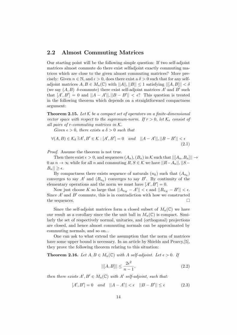
2.2 Almost Commuting Matrices

Our starting point will be the following simple question: If two self-adjointmatrices almost commute do there exist selfadjoint exactly commuting ma-trices which are close to the given almost commuting matrices? More pre-cisely: Given n ∈ N, and ε > 0, does there exist a δ > 0 such that for any self-adjoint matrices A,B ∈ Mn(C) with ||A||, ||B|| ≤ 1 satisfying ||[A,B]|| < δ(we say (A,B) δ-commute) there exist self-adjoint matrices A′ and B′ suchthat [A′, B′] = 0 and ||A − A′||, ||B − B′|| < ε? This question is treatedin the following theorem which depends on a straightforward compactnessargument:

Theorem 2.15. Let K be a compact set of operators on a finite-dimensionalvector space with respect to the supremum-norm. If r > 0, let Kr consist ofall pairs of r-commuting matrices in K.

Given ε > 0, there exists a δ > 0 such that

∀(A,B) ∈ Kδ ∃A′, B′ ∈ K : [A′, B′] = 0 and ||A−A′||, ||B −B′|| < ε(2.1)

Proof. Assume the theorem is not true.Then there exist ε > 0, and sequences (An), (Bn) inK such that ||[An, Bn]|| →

0 as n→∞ while for all n and commuting R,S ∈ K we have ||R−An||, ||S−Bn|| ≥ ε.

By compactness there exists sequence of naturals (nk) such that (Ank)converges to say A′ and (Bnk) converges to say B′. By continuity of theelementary operations and the norm we must have [A′, B′] = 0.

Now just choose K so large that ||AnK − A′|| < ε and ||BnK − B′|| < ε.Since A′ and B′ commute, this is in contradiction with how we constructedthe sequences.

Since the self-adjoint matrices form a closed subset of Mn(C) we haveour result as a corollary since the the unit ball in Mn(C) is compact. Simi-larly the set of respectively normal, unitaries, and (orthogonal) projectionsare closed, and hence almost commuting normals can be approximated bycommuting normals, and so on...

One can ask to what extend the assumption that the norm of matriceshave some upper bound is necessary. In an article by Shields and Pearcy,[5],they prove the following theorem relating to this situation:

Theorem 2.16. Let A,B ∈Mn(C) with A self-adjoint. Let ε > 0. If

||[A,B]|| ≤ 2ε2

n− 1, (2.2)

then there exists A′, B′ ∈Mn(C) with A′ self-adjoint, such that:

[A′, B′] = 0 and ||A−A′|| < ε ||B −B′|| ≤ ε (2.3)

14

Furthermore if B is self-afjoint, B′ can also be chosen to be self-adjoint.

We omit the proof, and instead go in a different direction. Noticehow the δ in Theorem 2.15 depends not only on ε but also on the di-mension of the Hilbert Space which the operators act on. We will nowask whether it is possible to choose the δ in the Theorem 2.15 indepen-dently on the dimension of the underlying Hilbert Space - we say then thatthe approximation is uniform. In this case we cannot use the compact-ness argument, and the problem becomes much harder. We will be inter-ested in the following natural questions: Are contractive almost commutingprojections/self-adjoints/unitaries/normals uniformly close to exactly com-muting projections/self-adjoints/unitaries/normals?

Projections

We start with simplest case of projections, and give a proof of the followingtheorem:

Theorem 2.17. Given ε > 0 there exists a δ > 0 such that for all positiveintegers n and any at most countable collection Ai ∈ Mn(C) of pairwiseδ-commuting projections there exists a pairwise commuting collection A′i ∈Mn(C) of projections such that ‖Ai −A′i‖ < ε.

Proof. Let us first reformulate the problem into a lifting problem. Let us justfor notational clarity consider the case of two almost commuting projections- the reformulation for countably many almost commuting projections isanalogous.

Assume the theorem is not true. Then there exist some ε > 0, andsequence of positive integers, and sequences of matrices (Pk), (Qk) ∈ Msuch that [π(Pk), π(Qk)] = 0, and for any commuting pair (P ′k), (Q

′k) ∈ M

we have ‖P ′k − Pk‖ > ε and ‖Q′k −Qk‖ > ε for all k ∈ N. In particular thismeans that π(P ′k) 6= π(Pk) and π(Q′k) 6= π(Qk).

In other words if the theorem is not true it establishes the existence of anat most countable family of mutually commuting projections in M/A whichcannot be lifted to commuting projections in M .

However this is exactly what we will show, that we can do, in a few stepsbelow:

Step 1 - A projection in M/A can be lifted to a projection in M : Letp = (pk) be a projection in M/A. Since p is self-adjoint it lifts to a self-adjoint s = (sk) ∈M . We have π(s2− s) = 0, and hence ‖(s2

k − sk)‖ → 0 ask →∞.

Choose N such that ‖(s2k−sk)‖ < 1/4 for k > N . Choose f as in Lemma

1.3.Let s′ = (s′k) be defined by s′k = sk for k > N , and sk = 0 for k ≤ N .

15

Let P = f(s′). This is clearly a projection, and

π(P ) = f(π(s)) = f(p) = p

Step 2 - Let p, x ∈M/A, where p is a projection and x is self-adjoint, forwhich [p, x] = 0. Then p lifts to a projection P , and x lifts to a self-adjointX, such that [P,X] = 0:

Lift p to a projection P , and lift x to a self-adjoint Y , and putX = (1− P )Y (1− P ) + PY P . Then:

π(X) = (1− p)x(1− p) + pxp = x(1− p) + xp = x,

and[P,X] = PXP − PXP = 0.

Step 3 - Let p, q ∈ M/A be projections such that [p, q] = 0. Then p andq lift to projections P and Q respectively such that [P,Q] = 0:

First lift p and q to a projection P and a self-adjoint X respectively,such that [P,X] = 0. Now use the procedure as in step 1 to X to obtain aprojection Q which is a lift of q. Since this Q will be a continuous functionof element with which P commutes, P will also commute with Q.

Step 4 - Let p1, . . . , pN ∈ M/A, be a finite family of mutually com-muting projections which can be lifted to mutually commuting projectionsP1, . . . , PN ∈M , and let q be a projection which commutes with all p1, . . . , pN ,then q can be lifted to a projection Q ∈M which commutes with all P1, . . . , PN .

Lift q to a selfadjoint Y , and now putX1 = (1− P1)Y (1− P1) + P1Y P1, andXk = (1 − Pk)Xk−1(1 − Pk) + PkXk−1Pk, for 2 ≤ k ≤ N . Let X := XN .By induction it is easy to see that each π(Xk) = Q, and [Xk, Pl] = 0 for1 ≤ l ≤ k ≤ N (but it is tedious to write down). Proceeding with X as instep 3, we obtain our desired projection Q.

In the proof above we showed the nice result that projections can belifted to projections from M/A. This is not in general true for other quotientalgebras.

The question remains whether it is always possible to lift an uncountablefamily of commuting projections to a family of commuting projections.3

Self-adjoints

In the case of self-adjoint matrices we have Lin’s Theorem [1]:

3The answer is not known to me at the time of writing this (EDIT: Now it is known tome - it is in general not possible to lift an uncountable family of commuting projectionsto an uncountable family of commuting projections).

16

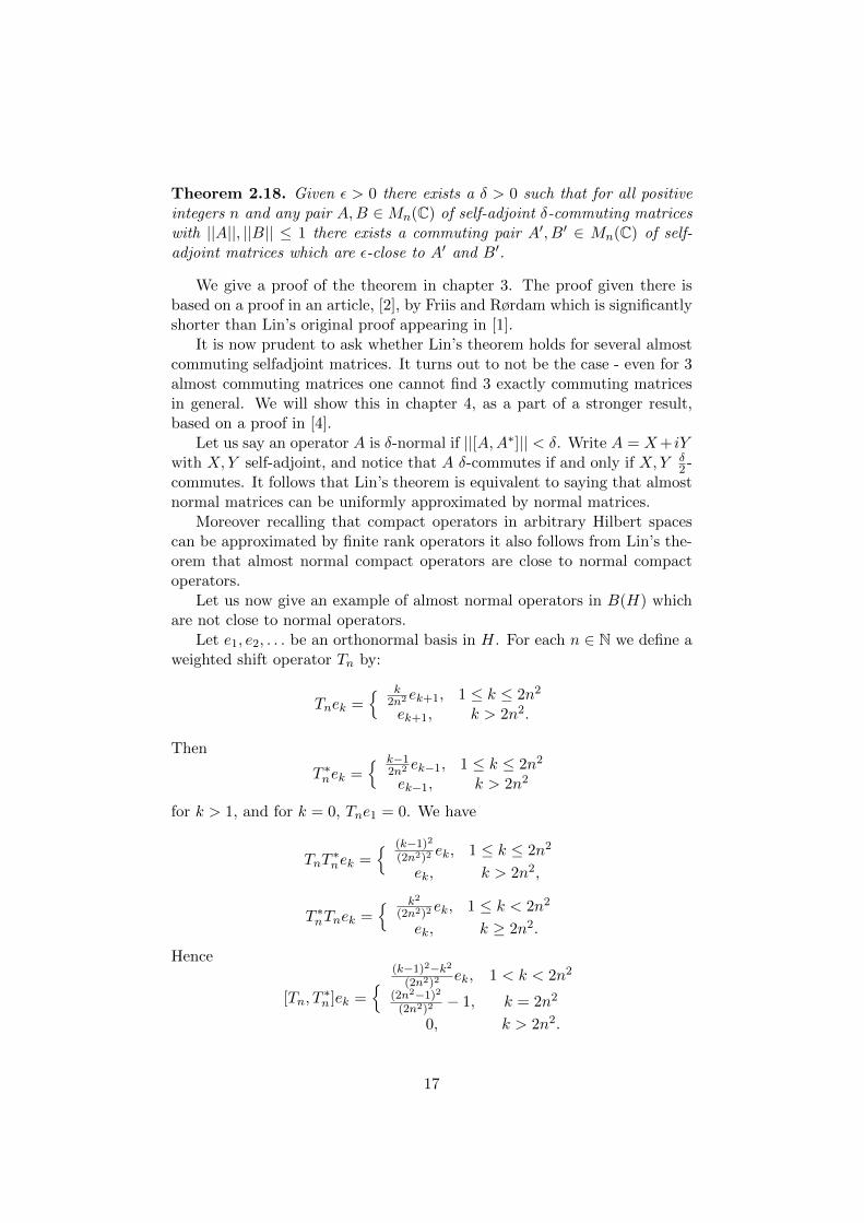
Theorem 2.18. Given ε > 0 there exists a δ > 0 such that for all positiveintegers n and any pair A,B ∈Mn(C) of self-adjoint δ-commuting matriceswith ||A||, ||B|| ≤ 1 there exists a commuting pair A′, B′ ∈ Mn(C) of self-adjoint matrices which are ε-close to A′ and B′.

We give a proof of the theorem in chapter 3. The proof given there isbased on a proof in an article, [2], by Friis and Rørdam which is significantlyshorter than Lin’s original proof appearing in [1].

It is now prudent to ask whether Lin’s theorem holds for several almostcommuting selfadjoint matrices. It turns out to not be the case - even for 3almost commuting matrices one cannot find 3 exactly commuting matricesin general. We will show this in chapter 4, as a part of a stronger result,based on a proof in [4].

Let us say an operator A is δ-normal if ||[A,A∗]|| < δ. Write A = X+ iYwith X,Y self-adjoint, and notice that A δ-commutes if and only if X,Y δ

2 -commutes. It follows that Lin’s theorem is equivalent to saying that almostnormal matrices can be uniformly approximated by normal matrices.

Moreover recalling that compact operators in arbitrary Hilbert spacescan be approximated by finite rank operators it also follows from Lin’s the-orem that almost normal compact operators are close to normal compactoperators.

Let us now give an example of almost normal operators in B(H) whichare not close to normal operators.

Let e1, e2, . . . be an orthonormal basis in H. For each n ∈ N we define aweighted shift operator Tn by:

Tnek = k

2n2 ek+1, 1 ≤ k ≤ 2n2

ek+1, k > 2n2.

Then

T ∗nek = k−1

2n2 ek−1, 1 ≤ k ≤ 2n2

ek−1, k > 2n2

for k > 1, and for k = 0, Tne1 = 0. We have

TnT∗nek =

(k−1)2

(2n2)2 ek, 1 ≤ k ≤ 2n2

ek, k > 2n2,

T ∗nTnek = k2

(2n2)2 ek, 1 ≤ k < 2n2

ek, k ≥ 2n2.

Hence

[Tn, T∗n ]ek =

(k−1)2−k2

(2n2)2 ek, 1 < k < 2n2

(2n2−1)2

(2n2)2 − 1, k = 2n2

0, k > 2n2.

17

Since

|(2n2 − 1)2

(2n2)2− 1| < 1

n2

and

|(k − 1)2 − k2

(2n2)2| < 1

n2

for all k < 2n2, we obtain

‖[Tn, T ∗n ]‖ < 1

n2→ 0

as n → ∞. Thus the operators Tn are almost normal. We claim that theyare not close to any normal operators. Suppose they were. Then there wouldexist normal operators Nn such that

Tn −Nn → 0. (2.4)

Since all Tn are compact perturbations of the unilateral shift, we have

index Tn = −1

for all n.From the remark after Theorem 2.13, (2.4) it follows that for n large

enough Nn is Fredholm of index −1. But any normal Fredholm operatorhas index 0. This gives a contradiction.

Unitaries and Normals

It is interesting that the same question for unitary matrices comes with anegative answer:

Theorem 2.19. There exist pairs (An, Bn)n∈N of unitary operators, An, Bn ∈Mn(C) such that ||[An, Bn]|| → 0 as n → ∞ and such that max||A′ −An||, ||B′ − Bn|| ≥ c for some positive c for all positive integers n and allcommuting matrices A′, and B′ (of the appropriate dimension).

In chapter 4 we give an explicit example (called Voiculescu’s pair) basedon the short article, [3], by Loring and Exel. The argument depends ona topological obstruction involving winding numbers. Since unitaries arenormal the question is already answered in the negative above with theVoiculescu pair. Notice that the Voiculescu pair cannot be approximated byany commuting matrices (they need not be unitary, not even normal).

18

2.3 Quasidiagonal Operators and The Weyl-vonNeummann-Berg Theorem

Now let us consider the validity of Theorem 1.1 for non-compact normaloperators. We will show the following theorem relating this question:

Theorem 2.20. Let H be a separable Hilbert space, and let A be a normaloperator on H. Given ε > 0. There exists a diagonal operator, D, and acompact operator, K such that A = D +K, where ‖K‖ < ε.

We will use Lin’s Theorem to prove this result. Before this we willhowever need to introduce quasidiagonal operators and discuss some funda-mental properties of these. This will also be useful in chapter 5.

Quasidiagonal Operators

We define the following:

Definition 2.21. We say T ∈ B(H) is blockdiagonal if and only if thereexists an increasing sequence of finite rank projections (Pn) which convergesto I in the strong operator topology such that [T, Pn] = 0 for all n ∈ N.

In particular if the rank of Pn−Pn−1 is 1 for positive integers n, T in thedefinition is diagonal (We here define block diagonal and diagonal withoutreference to any particular basis - thus diagonalizeable, and blockdiagonal-izeable might be more appropriate words).

Definition 2.22. We say an operator T ∈ B(H) is quasidiagonal if and onlyif there exist an increasing sequence of finite rank projections (Pn) whichconverges to I in the strong operator topology such that ‖[T, Pn]‖ → 0 forn→∞.

Actually what we call quasidiagonal would make more sense if we calledit quasi-block-diagonal. We also have an equivalent so called local definition:

Local Definition 2.23. An operator T ∈ B(H) is quasidiagonal if and onlyif for any ε > 0, and for any finite rank projection E there exists a finiterank projection F ≥ E such that ‖[F, T ]‖ < ε.

Proof. First we prove the if part of the theorem. Let (En) be any increasingsequence of finite rank projections which converge to I in SOT. Choose afinite rank projection F1 such that F1 ≥ E1. For n > 1 let Fn be the finiterank projection onto the subspace spanned by the ranges of En and Fn−1 andchoose a finite rank projection Fn such that Fn ≥ Fn and ‖[Fn, T ]‖ < 1/n.By construction (Fn) is an increasing sequence of finite rank projections -we only need to show they converge strongly to I. Let x ∈ H. Then:

‖Fnx− x‖ ≤ ‖Fnx−FnEnx‖+ ‖FnEnx− x‖ = ‖Fn(1−En)x‖+ ‖Enx− x‖

19

Since En converges strongly to 0, ‖Enx−x‖ → 0, and since ‖Fn(1−En)x‖ ≤‖(1− En)x‖, ‖Fn(1− En)x‖ → 0.

To see the only if part, let ε > 0, and E be a finite rank projection.Let (ei), i = 1 . . . , N , be an orthonormal basis for the range of E. Sincethere are finitely many ei there exist a finite rank projection P such that‖Pei − ei‖ < ε/N for all 1 ≤ i ≤ N and ‖[P, T ]‖ < ε. Let x ∈ H be a unitvector, then ‖Ex‖ ≤ 1. Writing Ex as a linear combination of the ei we seethat ‖PEx− Ex‖ ≤ ε. Hence ‖PE − E‖ ≤ ε.

Put Q = 1 − P . Then Q is a projection with finite codimension, suchthat ‖[T,Q] < ε‖ and ‖QE‖ < ε. Put Y = (1 − E)Q(1 − E). Then Y isselfadjoint, and Y E = 0. We now have:

‖Y −Q‖ = ‖ −QE − EQ(1− E)‖ ≤ 2ε

And we therefore have ‖Y ‖ ≤ 1 + 2ε, and hence also:

‖Y 2 −Q2‖ ≤ ‖Y 2 − Y Q‖+ ‖Y Q−Q2‖≤ ‖Y ‖‖Y −Q‖+ ‖Y −Q‖‖Q‖≤ 4ε+ 4ε2

So:‖Y 2 − Y ‖ = ‖Y 2 −Q2 +Q− Y ‖ ≤ 6ε+ 4ε2

Without loss of generality assume that ε is smaller that 1/4. Choose f asin Lemma 1.3 then f(Y ) is a projection satisfying ‖f(Y ) − Q‖ ≤ ‖f(Y ) −Y ‖ + ‖Y − Q‖ < ε′, where ε′ depends on ε in such a way it tends to 0 asepsilon tends to 0.

Let F = I − f(Y ). We must show F has the desired propertiesThat F is of finite rank follows from f(Y ) and Q having same co-

dimension, since ‖f(Y )−Q‖ < 1.Since f(0) = 0 we can find a sequnce of polynomials (pn) converging

uniformly to f such pn(0) = 0 for all n, Hence we can write pn(t) = tqn(t)for appropriate qn. Hence f(Y )E = limn→∞ qn(Y )Y E = 0. So F ≥ E.

Finally we have:

‖[T, F ]‖ = ‖[T, f(Y )]‖ ≤ ‖[T, f(Y )−Q]‖+ ‖[T,Q]‖ ≤ 2‖T‖ε′ + ε

Let us show the following fundamental result:

Theorem 2.24. An operator T ∈ B(H) is quasidiagonal if and only if it isa compact perturbation of a blockdiagonal operator.

Proof. To see the only if part, let T be quasidiagonal, and let (Pn) be a in-creasing sequence of finite rank procetions such that ‖[T, Pn]‖ → 0. Choose a

20

subsequence (Qn) of (Pn) such that ‖[T,Qn]‖ < 2−n, then∑∞

n=1 ‖[Qn, T ]‖ <∞. Let Q0 = 0, and let S be the blockdiagonal operator

∑∞n=1(Qn −

Qn−1)T (Qn −Qn−1). Now since T =∑∞

n=1(Qn −Qn−1)T , we have:

T − S =

∞∑n=1

−(Qn −Qn−1)[T,Qn] +

∞∑n=1

(Qn −Qn−1)[T,Qn−1]

Since each of sums converge in norm (since∑∞

n=1 ‖[Qn, T ]‖ < ∞) and theterms are compact operators, the limit must be compact since the set ofcompact operators is closed.

The if part of the theorem is obvious.

Remark: It follows from the proof above that if we start the subsequence(Qn) such that ‖[T,Qn]‖ < C for all n, then for the compact perturbationT −S we get ‖T −S‖ < 4C. Hence we can choose the compact perturbationto be arbitrary small.

It now follows:

Corollary 2.25. The set of quasidiagonal operators is closed under takingcompact perturbations.

We also have:

Theorem 2.26. The set of quasidiagonal operators is closed in the normtopology.

Proof. We will use the local definition of a quasidiagonality described inTheorem 2.23.

Let (Tn) be a sequence of quasidiagonal operators that converges to anoperator T . We must show that T is quasidiagonal. Let ε > 0 and let E bea finite rank projection.

Choose N such that ‖TN−T‖ < ε. Since TN is quasidiagonal there existsa finite rank projection F ≥ E such that ‖[TN , F ]‖ < ε. We now have:

‖[T, F ]‖ ≤ ‖[T − TN , F ]‖+ ‖[TN , F ]‖ ≤ 3ε

Lemma 2.27. Every normal operator in B(H) is quasidiagonal.

Proof. Every normal operator in B(H) can be approximated by a normaloperator with finite spectrum by Lemma 1.2. Since every normal operatorwith finite spectrum is quasidiagonal (by spectral theorem), and since theset of quasidiagonal operators is closed by Theorem 2.26, we conclude thatnormal operators in B(H) are quasidiagonal.

21

Proof of the Weyl-von Neumann-Berg Theorem using Lin’sTheorem

Let N be a normal operator. We want to write it as a diagonal plus anarbitrary small compact operator. Let ε > 0.

By Lemma 2.27 N is quasidiagonal, and by Theorem 2.24 we can writeN = B+K where B is blockdiagonal, and K is compact, and by the remarkafter Theorem 2.24 we can choose ‖K‖ < ε.

Write B =∑∞

n=1Bn, where Bn = (Pn − Pn−1)B(Pn − Pn−1), and (Pn)is a increasing sequence of finite rank projections converging strongly to I,and P0 = 0.

Since N is normal we have 0 = [N,N∗] = [B,B∗] + K ′, where K ′ isa compact operator (since the compact operators form a two-sided ideal),with ‖K ′‖ < ε′ where ε′ tends to zero as ε tends to zero.

Now ‖[Bn, B∗n]‖ → 0, since [B,B∗] = −K ′ is compact.4 Moreover each‖[Bn, B∗n]‖ ≤ ‖K ′‖. By Lin’s Theorem we can choose a sequence of normaloperators Dn satisfying Dn = (Pn − Pn−1)Dn(Pn − Pn−1), such that ‖Bn −Dn‖ → 0, and ‖Bn −Dn‖ < ε′′ where ε′′ tends to zero as ε tends to zero.

Put K ′′ =∑∞

n=1(Bn −Dn) which is clearly compact.Put D =

∑∞n=1Dn. Since each Dn can be considered as a normal oper-

ator on a finite dimensional Hilbert space, D is clearly diagonal.We now have:N = D +K ′′ +K, where ‖K ′′ +K‖ ≤ ε+ ε′′.This completes the proof.

4To see this: Assume the supremum norm of the blocks do not tend to 0. Then we canchoose a sequence of unit vectors all belonging to different blocks such that their imagesare mutually orthogonal and has norm greater than some fixed positive real number. Thissequence clearly does not have a convergent subsequence which contradicts with the imageof the unit ball being precompact.

22

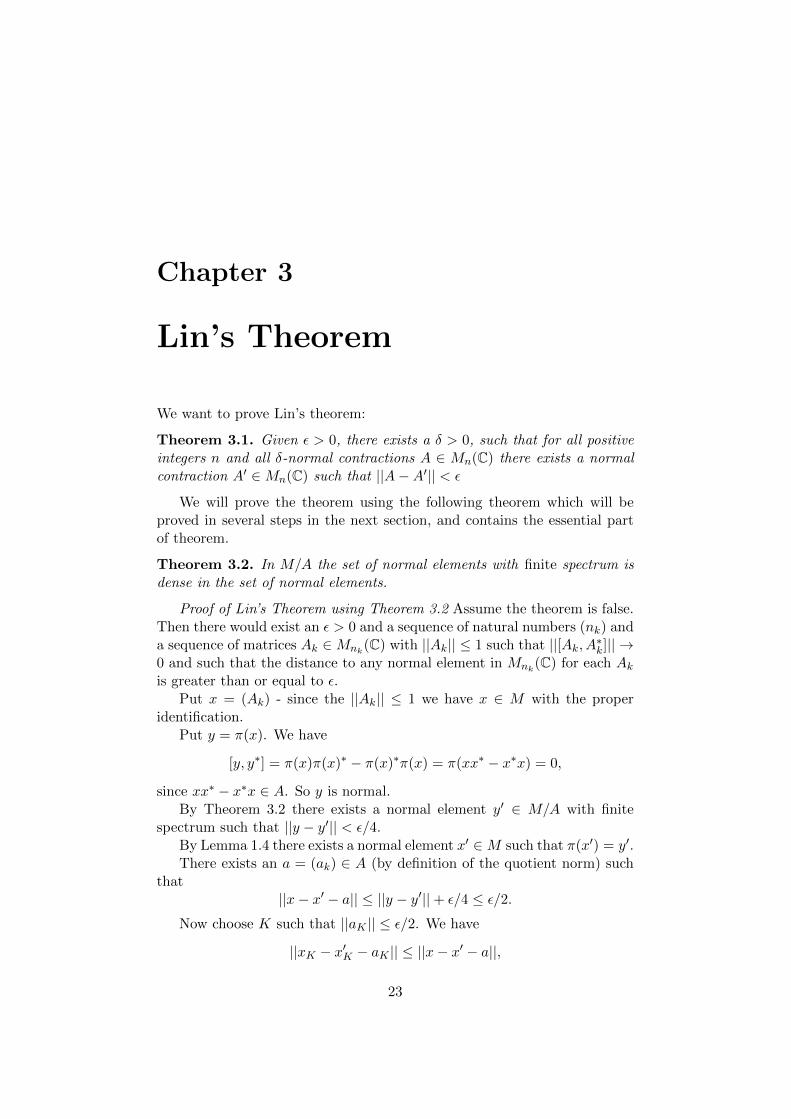
Chapter 3

Lin’s Theorem

We want to prove Lin’s theorem:

Theorem 3.1. Given ε > 0, there exists a δ > 0, such that for all positiveintegers n and all δ-normal contractions A ∈ Mn(C) there exists a normalcontraction A′ ∈Mn(C) such that ||A−A′|| < ε

We will prove the theorem using the following theorem which will beproved in several steps in the next section, and contains the essential partof theorem.

Theorem 3.2. In M/A the set of normal elements with finite spectrum isdense in the set of normal elements.

Proof of Lin’s Theorem using Theorem 3.2 Assume the theorem is false.Then there would exist an ε > 0 and a sequence of natural numbers (nk) anda sequence of matrices Ak ∈Mnk(C) with ||Ak|| ≤ 1 such that ||[Ak, A∗k]|| →0 and such that the distance to any normal element in Mnk(C) for each Akis greater than or equal to ε.

Put x = (Ak) - since the ||Ak|| ≤ 1 we have x ∈ M with the properidentification.

Put y = π(x). We have

[y, y∗] = π(x)π(x)∗ − π(x)∗π(x) = π(xx∗ − x∗x) = 0,

since xx∗ − x∗x ∈ A. So y is normal.By Theorem 3.2 there exists a normal element y′ ∈ M/A with finite

spectrum such that ||y − y′|| < ε/4.By Lemma 1.4 there exists a normal element x′ ∈M such that π(x′) = y′.There exists an a = (ak) ∈ A (by definition of the quotient norm) such

that||x− x′ − a|| ≤ ||y − y′||+ ε/4 ≤ ε/2.

Now choose K such that ||aK || ≤ ε/2. We have

||xK − x′K − aK || ≤ ||x− x′ − a||,

23

and by the reverse triangle inequality we get

||xK − x′K || < ε,

which is a contradiction.

3.1 Proof that the set of normal elements withfinite spectrum is dense in the set of normalelements in M/A

We will prove the theorem through a sequence of lemmas, starting with:

Lemma 3.3. Each element x ∈ M/A has a polar decomposition, x = u|x|,where u is unitary.

Proof. Let y = (yk) ∈M be any lift of x. For each positive integer n we haveyk = uk|yk| with uk unitary, since Cnk is finite dimensional. Put u = (uk),which is unitary. Now y = u|y|, and x = π(u)|x|, where π(u) is unitary sinceπ is a *- homomorphism.

Using unitary polar decomposition we will show the following:

Lemma 3.4. In M/A the set of invertible normal elements is dense in theset of normal elements.

Proof. Let x ∈M/A be normal. Let ε > 0.By Lemma 3.3 we can write x = u|x| where u ∈M/A is unitary.Since x is normal we have |x|2 = u|x|2u∗, hence |x|2 and u commute, and

hence |x| and u commute. Moreover |x|+ ε1 is invertible since it has strictlypostive spectrum. It follows that y = u(|x| + ε1) is normal and invertible,and moreover ||x− y|| = ε as desired.

Lemma 3.5. Let F ⊂ C be an at most countable set. The set of normalelements in M/A which have spectrum disjoint with F is dense in the set ofnormal elements in M/A.

Proof. Let Hλ be the set of normal elements in M/A which do not have λin the spectrum. The mapping x 7→ x−λ defined on the normal elements inM/A onto the normal elements is a homeomorphism for any λ ∈ C, which inparticular maps Hλ onto the set of invertible normal elements. By Lemma3.4 it follows that Hλ is dense in the set of normal elements.

Moreover Hλ is relatively open because the set of invertible normal ele-ments is relative open (and the set of invertible normal elements is relativelyopen since the set of invertible elements is open).

By the Baire Category theorem the set⋂λ∈F Fλ is dense in the set of

normal elements, which proves the lemma.

24

The results in Lemma 3.4 and 3.5 only depended on the existense of aunitary polar decomposition of normal elements.

For the next lemma we will introduce the following subsets of the complexplane (An ε-grid, and its center-points):

Γε := x+ iy ∈ C | x ∈ εZ or y ∈ εZ

Σε := x+ iy ∈ C | x ∈ ε(Z + 1/2) and y ∈ ε(Z + 1/2)

Lemma 3.6. For any normal element x ∈ M/A,and for any ε > 0 thereexists normal element y ∈M/A with σ(y) ⊂ Γε and ||x− y|| < ε.

Proof. Let x ∈ M/A By Lemma 3.5, since Σε is countable, there exists anx′ ∈M/A such that ||x− x′|| < ε(1− 1√

2), and σ(x′) ∩ Σε = ∅.

Let r : C\Σε → Γε be the continuous retraction defined as follows: Foreach c ∈ Σε, consider all lines from c until they intersect with the grid Γε- every point on such a line segment is mapped to where the line intersectswith the grid. We have: |r(z)− z| < 1√

2ε.

Now take y = r(x′) - we have ||y − x|| = ||f(x′) − x′ + x′ − x|| ≤||f(x′)− x′||+ ||x′ − x|| < ε.

Lemma 3.7. Let u ∈M/A be unitary. Then u can be lifted to a unitary inM .

Proof. Let π(a) = u. Since in matrix algebras all isometries are unitaries,we can write a = v|a|, where v is unitary. Now we have

u = π(a) = π(v|a|) = π(v)π(|a|) = π(v)|π(a)| = π(v).

Lemma 3.8. Let x ∈M/A be a normal element. Suppose V is a relativelyopen subset of σ(x), which is homeomorphic to an open interval. Then forany λ0 ∈ V and any ε > 0, there exists a normal element y ∈ M/A suchthat σ(y) ⊂ σ(x)\λ0 and ||x− y|| ≤ ε.

Proof. Let x ∈M/A be a normal element. Let U be a relatively open subsetof V (V as in the theorem statement), which satisfy: λ0 ∈ U ⊂ U ⊂ V , anddiam(U) < ε.

Let f0 be a homeomorphism from V onto T\−1, and extend it to acontinuous function f : σ(x)→ T by putting it equal to −1 everywhere else.Put u = f(x) which is unitary since its spectrum is contained in the unitcircle. By the Lemma 3.7 there exists a unitary v ∈M such that π(v) = u.

25

Let W = f(U) and let 1W be the characteristic function on W . SinceM is a von Neumann algebra 1W (v) is in M . Let e := π(1W (v)) which is aprojection in M/A.

Let ϕ : σ(x) → C be a continuous function which is 0 on σ(x)\V , andlet ϕ : T→ C be a (the) continuous function such that ϕ = ϕ f .

Since 1W (v) commutes with v, e = π(1W (v)) commutes with u = π(v),and hence e commutes with ϕ(x), since ϕ(x) = ϕ(u).

If ϕ = 1 on U , then ϕ = 1 on W , and then

1W (v)ϕ(v) = (1W ϕ)(v) = 1W (v),

meaning that

eϕ(x) = eϕ(u) = π(1W (v)ϕ(π(v)) = π(1W (v)ϕ(v)) = e.

If ϕ = 0 on σ(x)\U , then ϕ = 0 on T\W , and then

1W (v)ϕ(v) = (1W ϕ)(v) = ˆϕ(v),

meaning thateϕ(x) = ϕ(x).

Now let h : σ(x) → [0, 1] be continuous with h|U = 1 and h|σ(x)\V = 0.From the above considerations we have h(x)e = eh(x) = e, and since z 7→zh(z) vanishes on σ(x)\V we also have xh(x)e = exh(x). Hence

xe = xh(x)e = exh(x) = eh(x)x = ex

so x and e commute.We want to show that:

σe(M/A)e(exe) ⊂ U and σ(1−e)(M/A)(1−e)((1−e)x(1−e)) ⊂ σ(x)\U (3.1)

First we show σe(M/A)e(exe) ⊂ U . Let φ, ψ : σ(x)→ C be any continuousfunctions such that φ vanish on U and is equal to 1 on σ(x)\V , and ψ vanishon σ(x)\U . We now have (in the corner algebra eM/Ae)

φ(exe) = φ(xe) = φ(x)e = e− (1− φ(x))e = e− e = 0,

where we in the second last equality used that 1−φ is equal to 1 on U . Andwe also have (in the corner algebra (1− e)M/A(1− e))

ψ(x(1− e)) = ψ(x)(1− e) = ψ(x)− ψ(x)e = ψ(x)− ψ(x) = 0,

where we in the second last equality used that ψ vanishes on σ(x)\U . Thisshows 3.1.1

1Why? For instance assume some α ∈ U is in σ(1−e)(M/A)(1−e)((1− e)x(1− e)). Thenthere exists a continuous function ψα which is 1 at α, and which is 0 on σ(x)\U (forinstance by Urysohn’s lemma). Then ψα(xe) would have 1 in its spectrum and thenψα(xe) 6= 0.

26

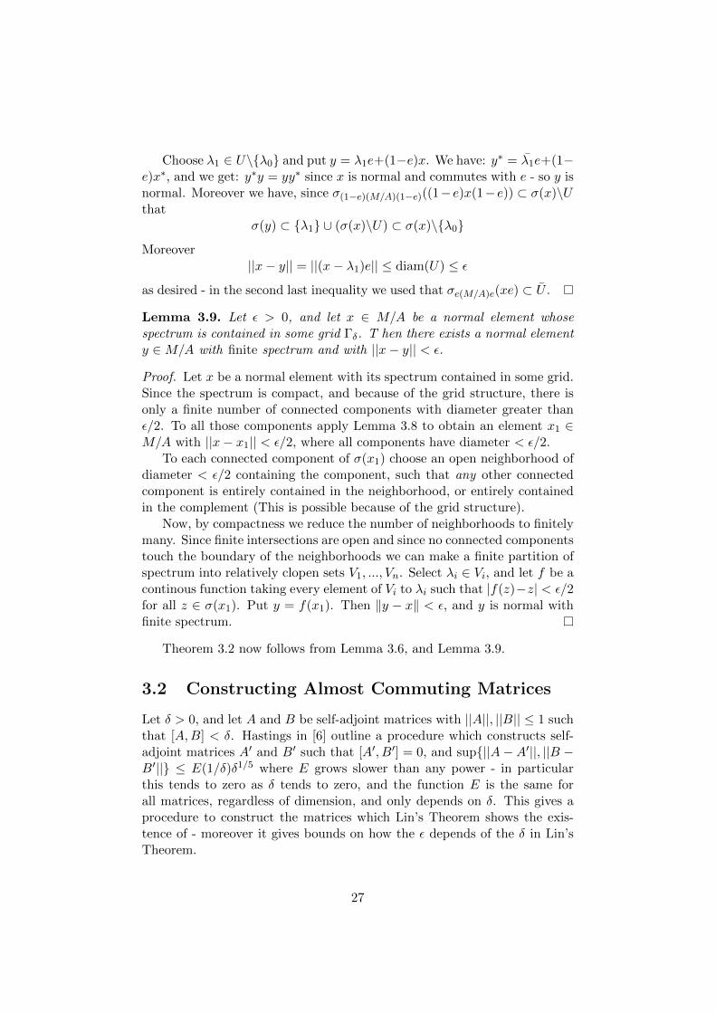
Choose λ1 ∈ U\λ0 and put y = λ1e+(1−e)x. We have: y∗ = λ1e+(1−e)x∗, and we get: y∗y = yy∗ since x is normal and commutes with e - so y isnormal. Moreover we have, since σ(1−e)(M/A)(1−e)((1−e)x(1−e)) ⊂ σ(x)\Uthat

σ(y) ⊂ λ1 ∪ (σ(x)\U) ⊂ σ(x)\λ0

Moreover||x− y|| = ||(x− λ1)e|| ≤ diam(U) ≤ ε

as desired - in the second last inequality we used that σe(M/A)e(xe) ⊂ U .

Lemma 3.9. Let ε > 0, and let x ∈ M/A be a normal element whosespectrum is contained in some grid Γδ. T hen there exists a normal elementy ∈M/A with finite spectrum and with ||x− y|| < ε.

Proof. Let x be a normal element with its spectrum contained in some grid.Since the spectrum is compact, and because of the grid structure, there isonly a finite number of connected components with diameter greater thanε/2. To all those components apply Lemma 3.8 to obtain an element x1 ∈M/A with ||x− x1|| < ε/2, where all components have diameter < ε/2.

To each connected component of σ(x1) choose an open neighborhood ofdiameter < ε/2 containing the component, such that any other connectedcomponent is entirely contained in the neighborhood, or entirely containedin the complement (This is possible because of the grid structure).

Now, by compactness we reduce the number of neighborhoods to finitelymany. Since finite intersections are open and since no connected componentstouch the boundary of the neighborhoods we can make a finite partition ofspectrum into relatively clopen sets V1, ..., Vn. Select λi ∈ Vi, and let f be acontinous function taking every element of Vi to λi such that |f(z)−z| < ε/2for all z ∈ σ(x1). Put y = f(x1). Then ‖y − x‖ < ε, and y is normal withfinite spectrum.

Theorem 3.2 now follows from Lemma 3.6, and Lemma 3.9.

3.2 Constructing Almost Commuting Matrices

Let δ > 0, and let A and B be self-adjoint matrices with ||A||, ||B|| ≤ 1 suchthat [A,B] < δ. Hastings in [6] outline a procedure which constructs self-adjoint matrices A′ and B′ such that [A′, B′] = 0, and sup||A−A′||, ||B −B′|| ≤ E(1/δ)δ1/5 where E grows slower than any power - in particularthis tends to zero as δ tends to zero, and the function E is the same forall matrices, regardless of dimension, and only depends on δ. This gives aprocedure to construct the matrices which Lin’s Theorem shows the exis-tence of - moreover it gives bounds on how the ε depends of the δ in Lin’sTheorem.

27

We will outline some of Hasting’s procedure, and show two theoremswhich are used, which are interesting in themselves. We will however skipthe most involved part of the algorithm.2

STEP 1 Put ∆ = δ4/5. Construct a matrix H such that ||[H,B]|| ≤ δ with thefollowing properties:

(1A) ||A − H|| ≤ ε1 := c0δ/∆, where c0 is a constant specified inTheorem 3.10.

(1B) For any eigenvectors v1, v2 of B with eigenvalues x1 and x2 sat-isfying |x1 − x2| ≥ ∆, we have (v1, Hv2) = 0.

The construction is given below in Theorem 3.10 as well as proof ofthe claims.

STEP 2 Choose c ≥ −1 such that [−1, 1] has no point with distance greaterthan ∆/2 to the set Sc := (c+ ∆N0) ∩ [−1, 1]. Let

Q : [−1, 1]→ (c+ ∆N0) ∩ [−1, 1]

be defined by letting Q(x) be the number in Sc closest to x (taking thesmallest in case there are two possibilities with same distance), andput X = Q(B). We clearly have:

(2A) ||X −B|| ≤ ε2 := ∆/2

STEP 3 Change to an (ordered) orthonormal basis O such that B is diagonalwith increasing eigenvalues in this basis. In this basis impose a blockstructure such that to each element i in N ∈ N0|c+N∆ ∈ Sc corre-sponds the block leaving eigenspace of X with eigenvalue c+∆i invari-ant - we here admit blocks to be of dimension 0 if no such eigenspaceexists. In this block structure [X]O is blockdiagonal with each blockequal to a scalar (We shall call this a ‘block identity matrix’ usingHastings terminology), and [H]O is block tridiagonal due to property(1B).

STEP 4 Put ncut = ∆−1/4. For 0 ≤ i ≤ ncut−1, define Ii = [−1+2(j−1)/ncut[,for i = 1, ..., ncut − 1, and Ii = [−1 + 2(j − 1)/ncut] for i = ncut.Group the blocks defined in step 3 into ncut superblocks letting theith superblock consist of those blocks corresponding to eigenvalues ofX in the interval Ii. Let Ji correspond to the matrix representing the

2Hasting’s procedure is not our main goal in this text, and the steps are not alwaysso easy to follow, so we skip a lot here. The purpose of this section is just to mentionthis relatively new result, and emphasize the difference in having a constructive proof andnot having it. This entire section can be read as an (very) early attempt at making anexposition of Hasting’s article.

28

i-th superblock of H. That is: Ji is the matrix obtained by projectingH to the subspace Bi consisting of the eigenspaces of X correspondingto eigenvalues in the interval Ii. Each Ji consist of Li blocks whereLi ≥ b 2

ncut− 1c, and is block tridiagonal. Label the eigenspaces of

X constained in Bi by Vi,j in order of increasing eigenvalues (So eacheigenspace corresponds to a block).

STEP 5 For each 1 ≤ i ≤ ncut construct a subspace Wi of Bi, which explicitconstruction we will skip.

The subspace Wi will have the following properties.

(5A) The projection of any normalized vector v ∈ Vi,1 onto W⊥i hasnorm bounded by ε3 := 1

L1/3i

f3(Li), where f3 is a function growing

slower than any power.

(5B) For any normalized vector w ∈ Wi, the projection of Jiw ontoW⊥i has norm bounded by ε4 := 1

L1/3i

f4(Li), where f4 is a function

growing slower than any power.

(5C) The projection of any normalized vector v ∈ Vi,L onto Wi hasnorm bounded by ε5 := f5(Li), where f5 is a function decayingfaster than any power.

STEP 6 Let DBi be the dimension of Bi, and DWi be the dimension of Wi.For 1 ≤ i ≤ Li create orthnormalbasis pi,k, 1 ≤ k ≤ DWi of Wi, andorthonormalbasis qi,l, 1 ≤ l ≤ DBi − DWi for W⊥i . Change from oldbasis O into a new basis N with a ncut+ 1 blocks indexed with integer0 ≤ m ≤ ncut, where the the mth block consists of basis vectors ofW⊥mand thenWm+1 in the given order (HereW⊥0 andWncut+1 are empty).In the new basis [H]N will be block pentadiagonal, and [X]N will beblock diagonal.

STEP 7 In the new basis choose [A′]N = [H]N on the blocks in the diagonal,and 0 outside. And choose B′ in the in the new basis such that it is ablock identity matrix with the mth block equal to −1 + 2m

ncuttimes the

identity.

Now A′ and B′ commute, and the off diagonal blocks of [A′]N − [H]Nare bounded by 2(ε3 + ε4 + ε5) (blocks in the diagonals straight aboveand below the main diagonal), and ε3ε5 (blocks in the diagonals twoabove and two below the main diagonal). Moreover ‖B′−B‖ ≤ 2/ncut.

The matrices obtained in step 7 are the desired matrices. The partskipped, was the subspace constructions in step 5, which admittingly also isthe hardest part. Let us also remark that the proof that the algorithm worksactually depends on Lin’s Theorem (or rather a corollary to Lin’s theorem).The Theorem below deals with step 1, and is interesting in itself:

29

Theorem 3.10. Given self-adjoint matrices A,B ∈Mn(C), such that ‖[A,B]‖ ≤δ. Given ∆ > 0. Let f be a Schwartz-function, such that it’s Fourier trans-form f is supported in [−1, 1], and is even, and has f(0) = 1.

Put H = ∆∫∞−∞ exp(iBt)A exp(−iBt)f(∆t)dt.

Then H is self-adjoint, ‖H −A‖ ≤ δ∆

∫∞−∞ |tf(t)|, ‖H −B‖ ≤ δ, and for

any eigenvectors v, w of B with respective eigenvalues r and s, which satisfy|r − s| ≥ ∆, we have (v,Hw) = 0.

Proof. Since f is real and even f is real, and H is self-adjoint.Since, 1 = f(0) =

∫∞−∞ f(t)dt = ∆

∫∞−∞ f(∆t)dt, we have:

‖H −A‖ = ‖∆∫∞−∞(exp(iBt)A exp(−iBt)−A)f(∆t)dt‖, which is less than

or equal to: ∆∫∞−∞ ‖(exp(iBt)A exp(−iBt)−A)f(∆t)dt‖.3 Now, since

‖(exp(iBt)A exp(−iBt)−A)′(t)‖ = ‖[A,B]‖, we have have:‖(exp(iBt)A exp(−iBt)−A)‖ ≤ |t|‖[A,B]‖.4 Hence we have:‖H −A‖ ≤ ∆−1δ

∫ t0 |t||f(t)|dt

‖[H,B]‖ ≤ δ, since∫∞−∞ |f(t)|dt = 1 (???).

Let v, w be eigenvectors of B with eigenvalues r and s respectively, suchthat |r − s| ≥ ∆. We have:

(v,Hw) = (v,∆

∫ ∞−∞

exp(iBt)A exp(−iBt)f(∆t)dtw)

=

∫ ∞−∞

∆f(∆t)(v, exp(iBt)A exp(−iBt)w)dt

=

∫ ∞−∞

∆f(∆t)(exp(−iBt)v,A exp(−iBt)w)dt

=

∫ ∞−∞

∆f(∆t)ei(s−r)t(v,Aw)dt

=

∫ ∞−∞

f(t)eis−r∆tdt(v,Aw),

= f(r − s

∆)dt(v,Aw),

which shows the last property, since |s − r|/∆ ≥ 1, since f is zero outside[−∆,∆].

Let S be a finite set of real numbers, and B a self-adjoint operator. Wesay that a vector is supported on the set S for B if it is a linear combina-tion of eigenvectors of B with eigenvalues in S. By P (S,B) we mean the

3Of course we should be careful those elementary identies and inequalities actually holdfor matrices. So far everything we have used can justified straightforwardly by looking atRiemann sums of matrices.

4Too see this, let v(t) = A(t)e, with A(0) = 0, where e is a unit vector. Now v(t) =v(0) +

∫ t0v′(s)ds. So ‖v(t)‖ ≤

∫ t0‖A′(s)ds‖. This holds for all unit vectors, so ‖A(t)‖ ≤∫ t

0‖A′(s)‖ds.

30

orthogonal projection onto the subspace spanned by eigenvectors of B witheigenvalues in S. If T is another finite set of real numbers dist(S, T ) denotesminsinS,t∈T |s− t|.

We now end this section by showing the following theorem which is anexample of a so-called Lieb-Robinson bound (and is used in Hastings proof).

Theorem 3.11. Let H be a hermitian matrix with ‖H‖ ≤ 1, and let B bea self-adjoint matrix, and ∆ > 0 such that for any two eigenvectors v, wof B, with respective eigenvalues r and s satisfying |r − s| ≥ ∆, we have(v,Hw) = 0.

Let S1 and S2 be finite sets of real numbers, and let |t| ≤ dist(S1, S2)/vLR,where vLR = e2∆.5

Then for any v supported on set S1 for B, we have:

‖P (S2, B) exp(−iHt)v‖ ≤ e−dist(S1,S2)/∆‖v‖

Proof. First notice if v is supported on S1 for B, then Hv is supported ona set with distance less than or equal to ∆ to S1, because of the way H andB are constructed. Thus applying Hn to v is 0, when n is a postive integerless than m = dist(S1, S2)/∆. Thus expressing exp(iHt) by its powerseriesand applying it to v, we see that the first terms of P (S2, B) exp(−iHt)vvanish. The result will now follow from the following inequalities, which willbe explained below:

‖P (S2, B) exp(−iHt)v‖ ≤ ‖∑n≥m

(−it)n(Hn/n!)v‖

≤∑n≥m

(|t|n/n!)‖v‖

≤ 1

e

∑n≥m

(e|t|n)n‖v‖

≤ 1

e(e|t|m)m

1

1− e|t|m‖v‖

≤ e−dist(S1,S2)/∆

First inequality is obvious from the previous discussion.Second inequality follows from ‖H‖ ≤ 1, and the triangle inequality.Third inequality is the Stirling approximation, which gives: n! <

√2πn(ne )n.

Fourth (in-)equality is just a geometric series.In the last inequality notice 0 ≤ e|t|/m ≤ 1/e < 1, and hence 1

e (e|t|/m)m ≤e−m−1 ≤ e−dist(S1,S2)/∆, and 1

1−e|t|m ≤ 1.

5LR stands for Lieb-Robinson: vLR is a so-called Lieb-Robinson bound, which is some-thing that arises in the theory of many-body systems.

31

Chapter 4

Two Counterexamples

In this chapter we give two non-trivial counter examples of failures in ap-proximating almost commuting matrices.

4.1 A Topological Obstruction

We will now give an example of almost commuting unitary matrices whichcannot be uniformly approximated by commuting unitaries. The exampleis a so-called Voiculescu pair Sn, Ωn defined by:

Sn =

0 11 0

1 0. . .

. . .

1 0

and

Ωn =

ωn

ω2n

ω3n

. . .

ωnn

where ωn is the nth unit root e2πi/n.

We see immediately that the Voiculescu pair has the following elementaryproperties which are straightforward to verify:

Proposition 4.1. Let Ωn and Sn be defined as above, then

(a) ||[Ωn, Sn]|| = |1− ωn|, which tends to 0 as n tends to ∞.

(b) det(Ωn) = det(Sn) = (−1)n+1

32

(c) SnΩnS∗n = ωnΩn

We will prove that although ||[Ωn, Sn]|| → 0 one has:

Theorem 4.2. For any n ≥ 7 and any pair of commuting matrices X,Y ∈Mn(C) we have: max||X − Ωn||, ||Y − Sn|| ≥

√2− |1− ωn| − 1.

The argument makes use of a topological obstruction (the winding num-ber) and is reasonably short - it is based on [3]. The number n ≥ 7 is chosento insure

√2− |1− ωn| − 1 is positive.

Proof. First let us note that if a matrix is non-invertible then the distanceto any unitary is at least 1,1 so we will limit our attention to invertiblesfrom now on:

Let X,Y ∈Mn(C) be commuting invertibles and put

d = max||X − Ωn||, ||Y − Sn||.

We will assume d <√

2− |1− ωn| − 1 and obtain a contradiction.Let At = Ωn + t(X − Ωn), and Bt = Sn + t(Y − Sn) for t ∈ [0, 1].For each t ∈ [0, 1] let γt be the closed curve in the complex plane defined

byγt(r) = det((1− r)AtBt + rBtAt),

r ∈ [0, 1].First we will show that γt(r)is never 0. To do this we will show that

(1 − r)AtBt + rBtAt is invertible for all r and t in the unit interval, byshowing ||(1 − r)AtBt + rBtAt − ΩnSn|| < 1. Since ΩnSn is unitary thisshows that ||(1 − r)AtBt + rBtAt|| is invertible. We find (by several timesusing the trick of adding and subtracting the same term):||(1− r)AtBt + rBtAt − ΩnSn||≤ (1− r)||AtBt − ΩnSn||+ r||BtAt − ΣnSn||≤ (1− r)(||AtBt −AtSn||+ ||AtSn − ΩnSn||)

+r(||BtAt − SnAt||+ ||SnAt − SnΩn||+ ||SnΩn − ΩnSn||)≤ (1− r)(||At|| ||Bt − Sn||+ ||At − Ωn||)

+r(||Bt − Sn|| ||At||+ ||At − Ωn||+ |1− ωn|)≤ (1− r)((1 + d)d+ d) + r((1 + d)d+ d+ |1−ωn|) = d2 + 2d+ r|1−ωn|≤ d2 + 2d+ |1− ωn| < 1.Since this complex curve is never 0, we will now look at the winding

number around 0 for different t. Since the winding number is a homotopyinvariant it should be the same for all t. Now, for t = 0 we have At = Ωn

and Bt = Sn and hence:

1Let ||U −X|| < 1 with U unitary. We have ||U −X|| = ||U(1−U∗X)|| = ||1−U∗X||.By a standard theorem in Banach algebras U∗X is invertible - hence X is invertible, sinceU is.

33

γ0(r) = det((1− r)ΩnSn + rSnΩn)

= det(Sn((1− r)ΩnSn + rSnΩn)S∗n)

= det(Sn) det((1− r)Ωn + rωnΩn)

= (−1)n+1 det((1− r + rωn)Ωn)

= (−1)n+1(1− r + rωn)n(−1)n+1

= (1− r + rωn)n

As r goes from 0 to 1, (1− r+ rωn) goes from 1 to ωn along the straightline segment connecting those two points. Thinking about polar coordinateswe see that curve, γ0 winds once in the clockwise direction around 0 in thecomplex plane.

For t = 1 we have At = X and Bt = Y which commute, so γt is constantand non-zero - and the winding number is 0.

Since the winding number is a homotopy invariant we have obtained acontradiction.

4.2 Three Almost Commuting Matrices

In this section we give an example constructed by Davidson of 3 almost com-muting self-adjoints which are not close to exactly commuting self-adjoints(Actually the counterexample is even stronger). Namely we will constructtwo sequences (An), (Bn) of matrices which are respectively self-adjoint andnormal, such that

[An, Bn]→ 0

while there are no matrices A′n = A′∗n and B′n (B′n not necessarily normal!)such that

[A′n, B′n] = 0, An −A′n → 0, Bn −B′n → 0.

We will need three auxiliary results. For the first one (Theorem 4.4below), in [4] it is given a reference to a paper of Voiculescu where it iscalled a folk theorem.2

Lemma 4.3. Let T and S be self-adjoint operators in B(H). Suppose C1,C2 are closed intervals such that σ(S) ⊆ C1, σ(T ) ⊆ C2 and

dist(C1, C2) = a

Let LS, RT be the operators of left multiplication by S and right multiplica-tion by T respectively. Then

‖(LS −RT )−1‖ ≤ 1/a

2Being unable to find this paper, we give here our own proof.

34

Proof. Without loss of generality we can assume that z1 − z2 ≥ a for allz1 ∈ σ(S), z2 ∈ σ(T ). By shifting to a constant, we can assume that σ(T ) ⊂(−∞,−a/2], σ(S) ⊂ [a/2,∞).

Let us begin with the formula:∫ ∞0

exp(−tz)dt = 1/z

which is valid for all z > 0 and even for all z with <(z) > 0.Now we may apply both analytic functions (in left-hand side and in

right-hand side) to any operator X with σ(X) ⊂ z : <(z) > 0∫ ∞0

exp(−tX)dt = X−1. (4.1)

Let X = LS − RT . Since σ(RT ) = σ(T ), σ(LS) = σ(S), and since leftmultiplications and right multiplications commute we have

σ(X) ⊆ z1 − z2 |z1 ∈ σ(S), z2 ∈ σ(T ) ⊂ (0,∞).

Hence the formula (4.1) is valid for our X.Now

(LS −RT )−1 =

∫ ∞0

exp(−t(LS −RT ))dt =

∫ ∞0

exp(−tLS) exp(tRT )dt

(we used here that LS and RT commute).Applying this equality to an operator V ∈ B(H) and taking into account

that‖ exp(−tLS) exp(tRT )(V )‖ = ‖ exp(−tS)V exp(tT )‖≤ ‖V ‖ exp(−ta/2) exp(−ta/2) = ‖V ‖ exp(−ta),we get

‖(LS −RT )−1(V )‖ ≤ ‖V ‖∫ ∞

0exp(−ta)dt = ‖V ‖/a

We proved that‖(LS −RT )−1‖ ≤ 1/a

For a self adjoint operator T , let ET (C) denote the spectral projectionfor T corresponding to the set C.

Theorem 4.4. Let ε and a be positive constants, and let C1 and C2 be closedintervals with dist(C1, C2) ≥ a. For any pair of self-adjoint operators A andB satisfying ‖A−B‖ < aε, one has

‖EA(C1)EB(C2)‖ < ε.

35

Proof. Let us denote P = EA(C1) and Q = EB(C2) for short. Write A withrespect to the decomposition H = PH ⊕ (1− P )H as

A =

(A11 A12

A21 A22

)and B with respect to the decomposition H = QH ⊕ (1−Q)H as

B =

(B11 B12

B21 B22

)Let λ ∈ C1 and µ ∈ C2. Define S with respect to the decomposition H =PH ⊕ (1− P )H as

S =

(A11

λ

)and T with respect to the decomposition H = QH ⊕ (1−Q)H as

T =

(B11

µ

)Then

SP =

(A11

λ

)(1

0

)=

(A11

0

)= PAP,

QT =

(1

0

)(B11

µ

)=

(B11

0

)= QBQ,

and we have

‖(LS−RT )(PQ)‖ = ‖PAPQ−PQBQ‖ = ‖PAQ−PBQ‖ = ‖P (A−B)Q‖ ≤ ||A−B|| ≤ aε.

Since σ(S) ⊆ C1 and σ(T ) ⊆ C2, by Lemma 4.3

‖(LS −RT )−1‖ ≤ 1/a

Hence

‖PQ‖ ≤ ‖(LS −RT )−1‖‖(LS −RT )(PQ)‖ < (1/a)aε = ε

The second auxiliary result can be considered as stability of the relationE ≤ F ≤ G (E,F,G are projections) under small perturbations of themiddle part F .

For a projection F we use notation F⊥ = 1− F .

Lemma 4.5. Let ε > 0. If E,F ′ and G are projections with E ≤ G,‖EF ′⊥‖ < ε, and ‖F ′G⊥‖ < ε, then there is a projection F such that E ≤F ≤ G and ‖F ′ − F‖ ≤ 3ε.

36

Proof. Since the distance between any two projections is not larger than 1,we can assume ε ≤ 1/3. Let us decompose the Hilbert space as

H = EH ⊕ (G− E)H ⊕G⊥H.

With respect to this decomposition we will write F ′ as

F ′ =

F11 F12 F13

F21 F22 F23

F31 F32 F33

Since ‖EF ′⊥‖ < ε and

EF ′⊥ =

10

0

1− F11 −F12 −F13

−F21 1− F22 −F23

−F31 −F32 1− F33

=

1− F11 −F12 −F13

0 0 00 0 0

we get

‖1− F11‖ < ε, ‖F12‖ < ε, ‖F13‖ < ε. (4.2)

Since ‖F ′G⊥‖ < ε and

F ′G⊥ =

F11 F12 F13

F21 F22 F23

F31 F32 F33

00

1

=

0 0 F13

0 0 F23

0 0 F33

we get

‖F13‖ < ε, ‖F23‖ < ε, ‖F33‖ < ε. (4.3)

Since F ′ is a projection, we have F ′ = F ′∗ which implies

Fij = F ∗ji (4.4)

and F ′ = F ′2 which implies

F22 = (F ′2)22 = F21F12 + F 222 + F23F32 (4.5)

From (4.4) and (4.5) we obtain that F22 − F 222 ≥ 0 and ‖F22 − F 2

22‖ ≤ 2ε2.Since F22 ≥ 0, we conclude that σ(F22) ⊂ [0, 4ε2] ∪ [1− 4ε2, 1].

Since ε < 1/3, we have 4ε2 < 1/2 and hence there is a continuousfunction f on R such that f |[0,4ε2] = 0 and f |[1−4ε2,1] = 1. Then P = f(F22)is a projection and

‖F22 − P‖ ≤ supt∈[0,4ε2]∪[1−4ε2,1]

|f(t)− t| ≤ 4ε2 < ε (4.6)

Finally we define F as

F =

1P

0

.

37

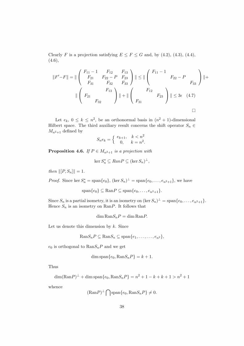
Clearly F is a projection satisfying E ≤ F ≤ G and, by (4.2), (4.3), (4.4),(4.6),

‖F ′−F‖ = ‖

F11 − 1 F12 F13

F21 F22 − P F23

F31 F32 F33

‖ ≤ ‖ F11 − 1

F22 − PF33

‖+‖

F13

F21

F32

‖+ ‖

F12

F23

F31

‖ ≤ 3ε (4.7)

Let ek, 0 ≤ k ≤ n2, be an orthonormal basis in (n2 + 1)-dimensionalHilbert space. The third auxiliary result concerns the shift operator Sn ∈Mn2+1 defined by

Snek = ek+1, k < n2

0, k = n2.

Proposition 4.6. If P ∈Mn2+1 is a projection with

kerS∗n ⊆ RanP ⊆ (kerSn)⊥,

then ‖[P, Sn]‖ = 1.

Proof. Since kerS∗n = spane0, (kerSn)⊥ = spane0, . . . , en2+1, we have

spane0 ⊆ RanP ⊆ spane0, . . . , en2+1.

Since Sn is a partial isometry, it is an isometry on (kerSn)⊥ = spane0, . . . , en2+1.Hence Sn is an isometry on RanP . It follows that

dim RanSnP = dim RanP.

Let us denote this dimension by k. Since

RanSnP ⊆ RanSn ⊆ spane1, . . . , . . . , en2,

e0 is orthogonal to RanSnP and we get

dim spane0,RanSnP = k + 1.

Thus

dim(RanP )⊥ + dim spane0,RanSnP = n2 + 1− k + k + 1 > n2 + 1

whence(RanP )⊥

⋂spane0,RanSnP 6= 0.

38

Hence there exists x ∈ spane0,RanSnP orthogonal to RanP . Since e0 ∈RanP , we have x ∈ RanSnP . It follows that x = SnPy, for some vector y.So SnPy is orthogonal to RanP , hence SnPy ∈ Ran(1− P ) and

(1− P )SnPy = SnPy.

Hence‖(1− P )SnPPy‖ = ‖SnPy‖ = ‖Py‖

(here the last equality holds since Sn is an isometry on RanP ). Thus

‖(1− P )SnP‖ ≥ 1. (4.8)

Now writing Sn with respect to the decomposition H = PH ⊕ (1− P )H

Sn =

(PSnP PSn(1− P )

(1− P )SnP (1− P )Sn(1− P )

)we obtain

[Sn, P ] =

(0 PSn(1− P )

(1− P )SnP 0)

).

By (4.8)

‖[Sn, P ]‖ = max‖PSn(1− P )‖, ‖(1− P )SnP‖ ≥ 1.

The opposite inequality is obvious.

Theorem 4.7. There exist finite rank matrices An, Bn, n ≥ 1, of norm1 such that An is self-adjoint, Bn is normal, and limn→∞‖[An, Bn]‖ = 0,yet there are no commuting pairs A′n, B

′n such that A′n is self-adjoint and

limn→∞ ‖An −A′n‖+ ‖Bn −B′n‖ = 0.

Proof. Define An and Bn in Mn2+1 as follows. Let ek, 0 ≤ k ≤ n2 be anorthonormal basis and let

Anek =k

n2ek, Bnek =

k+1n ek+1, 0 ≤ k < nek+1, n ≤ k ≤ n2 − n

n2−kn ek+1, n2 − n < k ≤ n2

(it is meant that Bnen2 = 0).Now An = A∗n, Bn is a weighted shift and it is straightforward to check

that‖[An, Bn]‖ = 1/n2 → 0.

Also one checks that limn→∞ ‖[Bn, B∗n]‖ = 0 and hence by Lin’s theoremthere are normal matrices Bn ∈ Mn2+1 such that limn→∞ ‖Bn − Bn‖ = 0.It means that we can use Bn for constructing the example.

39

In order to obtain a contradiction, we assume the existence of commutingpairs A′n, B

′n such that A′n is self-adjoint and

limn→∞

‖An −A′n‖+ ‖Bn −B′n‖ = 0. (4.9)

Let F ′n be the spectral projection of A′n for the interval [0, 1/2] and letEn and Gn be the spectral projections for An corresponding to the interval[0, 1/3] and [0, 2/3] respectively. Then from (4.9) and Theorem 4.4 it followsthat

limn→∞

‖EnF ′⊥n ‖ = 0 = limn→∞

‖F ′nG⊥n ‖

By Lemma 4.5 there exist projections Fn such that En ≤ Fn ≤ Gn and

limn→∞

‖Fn − F ′n‖ = 0. (4.10)

Since F ′n is a function of A′n and A′n commutes with B′n, we get [F ′n, B′n] = 0.

Now (4.9) and (4.10) imply that

limn→∞

‖[Fn, Bn]‖ = 0. (4.11)

Now we notice that on spanek, n ≤ k ≤ n2−n Bn acts as the shift operatorSn defined before Proposition 4.6. Since Gn −En is the spectral projectionfor An corresponding to the interval (1/3, 2/3] and since for the eigenvaluesk/n2 of An lying in the interval (1/3, 2/3] we have n < k < n2 − n for alln ≥ 4, we conclude that

Sn(Gn − En) = Bn(Gn − En) (4.12)

and(Gn − En)Sn = (Gn − En)Bn. (4.13)

Let us decompose the Hilbert space H = Cn2+1 as

H = EnH ⊕ (Gn − En)H ⊕G⊥nH

and write Sn and Fn with respect to this decomposition. Then (4.12) and(4.13) mean that

(Sn)12 = (Bn)12, (Sn)21 = (Bn)21, (Sn)22 = (Bn)22, (Sn)23 = (Bn)23, (Sn)32 = (Bn)32

(4.14)We notice also that by their constructions Bn and Sn do not have anythingin the right upper and left lower corners, so that

(Bn)13 = (Sn)13 = (Bn)31 = (Sn)31 = 0. (4.15)

Since En ≤ Fn ≤ Gn, we write Fn as

Fn =

1P

0

,

40

where P is a projection. Now using (4.14) and (4.15) we get

[Fn, Bn] =

0 (Bn)12(1− P ) 0

(P − 1)(Bn)21 [P, (Bn)22] P (Bn)23

0 −(Bn)32P 0

=

0 (Sn)12(1− P ) 0(P − 1)(Sn)21 [P, (Sn)22] P (Sn)23

0 −(Sn)32P 0

= [Fn, Sn]. (4.16)

This and (4.11) imply

limn→∞

[Fn, Sn] = 0.

But it is impossible because for any projection Q with

kerS∗n ⊆ ranQ ⊆ (kerSn)⊥

(in particular for Fn) one has ‖[Q,Sn]‖ ≥ 1. We obtained a contradiction.

41

Chapter 5

A BDF-Theorem

The goal is to prove, we recall:

Theorem 5.1. Let T ∈ B(H) be an essentially normal operator. Then Tis a compact perturbation of a normal operator if and only if T has trivialindex function.

The proof of 5.1 uses the following two results.

Theorem 5.2. Let A ∈ B(H). A is a compact perturbation of a normaloperator if and only A if is quasidiagonal and essentially normal.

Proof. By Lemma 2.27 every normal operator in B(H) is quasidiagonal.By corollary 2.25 compact perturbations of a normal operator is then alsoquasidiagonal, and clearly also essentially normal.

To prove the converse let T ∈ B(H) be quasidiagonal and essentiallynormal. By Theorem 2.24 T is a compact perturbation of a blockdiagonaloperator S =

∑∞n=1 Sn, where Sn = PnSPn, Pn = Qn − Qn−1, where (Qn)

increasing sequence of finite rank projections which converges to I in SOT,and Q0 = 0.

Since S is a compact perturbation of an essential normal operator S isitself essentially normal and we therefore have

∑∞n=1[Sn, S

∗n] is compact.

Hence ‖[Sn, S∗n]‖ → 0 since for any blockdiagonal compact operator thenorms of the individual blocks must tend to 0,1 moreover ‖Sn| ≤ ‖S‖, sowe can use Lin’s theorem to construct a sequence Rn of normal operators,where PnRnPn = Rn and ‖Rn−Sn‖ → 0. Putting R =

∑∞n=1Rn, it follows

R− S is compact, and R is normal. This shows the desired result.

Corollary 5.3. The set of compact perturbations of normal operators on His closed with respect to the norm topology.

1As in the proof of the Weyl-von Neumann-Berg theorem.

42

Proof. The set of compact perturbations of normal operators is the inter-section of two closed sets by Theorem 5.2. Namely, the set of quasidiagonaloperators (Theorem 2.26) and the set of essentially normal operators (Thepreimage of the closed set of normal elements in the Calkin-algebra).

Theorem 5.4. Let T ∈ Q(H) be normal. T is the norm limit of a sequenceof normal elements in Q(H) with finite spectrum if and only if T has trivialindex function.

The proof of this theorem will be given in section 5.1.

Proof of Theorem 5.1:Since a normal operator has index 0 and the index is invariant under

compact perturbations, every compact perturbation of a normal operatorhas trivial index function.

To see the other direction let T be an essentially normal with trivialindex function. Hence S := π(T ) is normal with trivial index function.By Theorem 5.4 there exists a sequence of normals with finite spectrum(Sn) ∈ Q(H) which converges to S in the norm topology, and lift (Sn)to (Tn) such that Tn converges to T in norm topology in B(H) (This ispossible because of the way the quotient norm is defined). Now, since everynormal element in the Calkin algebra with finite spectrum can be lifted to anormal element in B(H) by Lemma 1.4, we can choose a sequence of normaloperators Rn ∈ B(H), such that π(Rn) = Sn. Hence each Tn is a compactperturbation of a normal operator, and hence T is a compact perturbationof a normal operator by corollary 5.3.

5.1 Proof of Theorem 5.4

We will prove Theorem 5.4 through a sequence of lemmas in a similar waywe proved Lin’s theorem. The new thing is that the quotient is now theCalkin algebra, and we have to take into account the index.

Lemma 5.5. Let t ∈ Q(H) be a normal element, let λ ∈ σ(t), and let ε > 0.Then there exists a normal element s ∈ Q(H) satisfying: ‖t − s‖ ≤ 2ε,λ /∈ σ(s), index(s− λ) = 0, and σ(s)\B(λ, ε) = σ(t)\B(λ, ε).

Proof. Step 1 - Constructing s: Without loss of generality assume λ = 0.Let t ∈ Q(H) be normal and non-invertible, and let R be any lift of t suchthat π(R) = t. Then R has polar decomposition R = V |R|, and R∗ haspolar decomposition R∗ = V ∗|R∗|.

Let fε : [0;∞[→ [0,∞[ be the continuous function defined by fε(x) = 0,when x ≤ ε, and fε(x) = x− ε, when x > ε.

43

Consider V fε(|R|) and its adjoint V ∗fε(|R∗|).2 We want to show theyboth have infinite-dimensional kernels. Assume the spectral projection 1[0,ε](|R|)has finite rank. Then since (1[0,ε] + id)(|R|) is invertible, we get π(1[0,ε] +id)(|R|)) = |t| is invertible, and since t is normal this implies t invertible,which is a contradiction. So 1[0,ε](|R|) must have infinite-dimensional range.It now follows that fε(|R|) = fε(|R|)(1− 1[0,ε])(|R|) has infinite-dimensionalkernel. A similar argument shows V ∗fε(|R∗|) has infinite-dimensional ker-nel. Let Wfε(|R|) be the polar decomposition of V fε(|R|). Extend W to aunitary U such that V fε(|R|) = Ufε(|R|), which is possible since the kernelsof W and W ∗ have same cardinality (because they are infinite-dimensionaland H is assumed to be separable).

Let gε = fε + ε, and put

s = π(Ugε(|R|)) = π(V )fε(|t|) + π(U)ε.

Step 2 - Showing s has the desired properties: Since gε(|t|) and U areinvertible, s is invertible and index(s) = 0 because s lifts to an invertibleelement in B(H).

We also have

‖t− s‖ = ‖π(V )(|t| − fε(|t|))− π(U)ε‖ ≤ 2ε

To see s is normal, let β : [0,∞[→ [0,∞] be a continuous function suchthat fε(x) = xβ(x), and notice that

π(V )fε(|t|) = π(V )|t|β(|t|) = tβ(|t|)

is normal because it is a continuous function of t. We therefore havethat π(U)fε(|t|) = π(V )fε(|t|) is normal. It is now straightforward to see[π(U), fε(|t|)] = 0, and from this it is straightforward to see that s is normal.

Concerning the spectra, embed Q(H) into B(H ′) for some Hilbert spaceH ′. Write T for the image of t, and S for the image of s. Now we can useBorel function calculus inside B(H ′) to compare the spectra of s and t.

Put E = 1[0,ε](|T |). Then E clearly commutes with T , moreover Ecommutes with S, since S = γ(|T |), where γ is chosen such that γgε = 1[0,ε].

We now have T = TE + T (1− E) and S = SE + S(1− E), so we have

σ(T ) = σTE(TE) ∪ σT (1−E)(T (1− E))

andσ(S) = σSE(SE) ∪ σS(1−E)(S(1− E)).

We have σ(TE) = σ(T ) ∩B(0, ε), and σ(SE) = σ(S) ∩B(0, ε). So if wecan show T (1− E) = S(1− E) we are done.

2To see that fε(|R|)V ∗ = V ∗fε(|R∗|), show first this holds for polynomials, usingV |R| = V ∗|R∗|. Then take sequnce of polynomials converging uniformly to fε, and takelimit on both sides of the identity for the polynomials.

44

First notice that by expressing |S| and |E| as functions of |T | we have|S|(1 − E) = |T |(1 − E). Since |T | and 1 − E commute it is enough toshow K(1 − E) = 0, where K is the image of π(V ) − π(U) in B(H ′).Choose a sequence of bounded borel functions (hn) such that fεhn convergesmonotonicaly and pointwise to 1 − 1[0,ε]. Now since Kfε(|T |) = 0 we haveKfεhn(|T |) = 0,3 and hence K(1− E) = 0 as desired.

Lemma 5.6. Let F be a finite subset of C. The set LF ⊂ Q(H) of elements,S, for which S−λ is invertible and index(S−λ) = 0 for all λ ∈ F , is open.

Proof. Let λ ∈ F , then Lλ is open since the elements of index 0 constitutean open set in the Calkin algebra. Hence LF is open since it is a finiteintersection of open sets.

Lemma 5.7. Let F ⊂ C be finite. Then each normal element of Q(H) withtrivial index function can be approximated by a normal element, b ∈ Q(H),for which b− λ is invertible, and index(b− λ) = 0, for all λ ∈ F .

Proof. Let a ∈ Q(H) be normal with trivial index function. Enumerate theelements in F , such that F = λ1, . . . , λN, and F ∩ σ(a) = λi ∈ F |i ≥ K + 1.Given κ > 0, we want to find b ∈ Q(H) such that ‖a− b‖ ≤ κ, σ(b)∩F = ∅,and index(b− λi) = 0 for all 1 ≤ i ≤ N .

Inductively choose elements aK , aK+1, . . . , aN by letting aK = a, andchoose ak, for K + 1 ≤ k ≤ N , to be the normal element s obtained in 5.6with t = ak−1, λ = λk and ε = 1

2 minδ, d, κN−K , where the choice of δ and

d will be specified below.By Lemma 5.6 we choose δ such that index(ak−λi) = 0 for all 1 ≤ i ≤ k−

1 (Notice that T having trivial index function implies that index(aK−λi) = 0for 1 ≤ i ≤ K). Lemma 5.5 makes sure that we also have index(ak−λk) = 0.

Let d be the minimum distance between any points in F , it then followsthat λk, . . . , λN ∈ σ(ak).

Finally putting b = aN we have ||b− a|| ≤ κ.

Lemma 5.8. Let t ∈ Q(H) be a normal element with trivial index function,and let ε > 0. Then there exists a normal element s ∈ Q(H) with trivialindex function, σ(s) ⊂ Γε, and such that ‖s− t‖ ≤ ε.

Proof. Tactically choose N ∈ N such that Nε ≥ ‖t‖ + ε/4, and let X =x + iy ∈ C | |x|, |y| ≤ Nε. Loosely speaking X is a quadratic box madeup of ε-cells which boundaries are in the grid Γε, and contains the spectrumof any element with norm less than or ‖t‖+ ε/4. Applying Lemma 5.7 on twith F = Σε ∩X we obtain a normal a ∈ Q(H) such that: ‖a − t‖ ≤ ε/4,σ(a) ∩ (Σε ∩X) = ∅, index(a− λ) = 0 for all λ ∈ Σε ∩X. By the choice ofN we also have σ(a) ⊂ X\Σε.

3See for instance [9] or [10]

45

Put Y = X\Σε. Let r be as in the proof of Lemma 3.6 but restricted toY . Put s = r(a), which is normal with spectrum σ(s) ⊂ Γε ∩ X, and has‖t− s‖ ≤ ε/4 + 1√

2≤ ε.

It remains to be shown that if λ ∈ C\σ(s), then index(s−λ) = 0. If λ isin the unbounded component this is obvious, otherwise λ will be in the samecomponent as some µ ∈ Σε ∩X, and we have index(s − λ) = index(s − µ).Moreover there exists a continuous path of continuous functions ft : Y → Ysuch that f0 is the identity, and f1 = r (For instance a deformation retractionalong the line segments discussed in the definition of r in Lemma 3.6), sowe have index(s− µ) = index(a− µ) = 0.

Lemma 5.9. Let X be a compact subset of Γε for some ε > 0. Everycontinuous map f : X → C\0 is homotopic inside C(X,C\0) to a mapof the form

z 7→ (z − λ1)n1 · · · (z − λk)nk , (5.1)

where λi ∈ C\X and ni ∈ Z.

Proof. Choose N ∈ N such that X ⊂ [−Nε,Nε]2, and put Y = Γε ∩[−Nε,Nε]2. Extend f to a continuous function g : Y → C\0.4

Let C1, . . . , C4N2 be the the bounded connected components of C\Y .For 1 ≤ i ≤ 4N2, let γi be the simple closed curve with image Bi = Ci\Ciwith positive orientation, let ni be the winding number of h with respect toγi, choose λi ∈ Ci, and define:

h : Y → C\0 byh(z) = (z − λ1)−n1 · · · (z − λ4N2)n4N2g(z)

The winding number of h around γi is now 0. This means that h|Bi can bewritten as r(z)eiθ(z), where r is a continuous positive real function which isnever 0, and θ is a continuous real function.5 This means we can extendhBi to a continuous function on the whole of Ci which has image containedin C\0.6 Repeating this for all cells we get a continuous extension h :[Nε,Nε]2 → C\0 of h.

Since [Nε,Nε]2 is contractible, h is homotopic to the constant function1 inside C([Nε,Nε]2,C\0). Restricting the functions in the homotopy toX we obtain the desired result.

4Start by putting g(x) = 1 when x is a crosshairpoint of Y which is not in X. To seeg can be extended to the whole Y , consider a closed subset, C of [0, 1] which includes theendpoints where a continuous function h is defined and non-sero. The complement is thena collection of disjoint open intervals (ai, bi) where h(ai) and h(bi) are not 0. To extendh continuosly to the whole [0, 1] so the extension is different from 0 everywhere we justchoose for each i a continuous curve in C connecting h(ai) and h(bi) which does not gothrough 0.

5θ can be chosen continuous since since the winding number is zero.6To see this, let for instance r0 and θ0 be the minimums of r, and θ on Bi respectively.

Set the function equal to r0eiθ0 in the centerpoint of Ci. On the ‘radial’ line segments

from the center to the boundary make r and θ straight lines.

46

Lemma 5.10. Suppose u ∈ Q(H) is unitary with index(u) = 0. Then ucan be lifted to a unitary U ∈ B(H).

Proof. Let V be any lift of u. Then indexV = 0 and hence kerV and kerV ∗

have the same (finite) dimensions. Hence in its polar decomposition, thepartial isometry can be extended to unitary. So V = U |V | where U isunitary. Applying π on both sides we have u = π(U)|u| = π(U).

Lemma 5.11. Let t ∈ Q(H) be normal with trivial index function, andwith σ(t) ⊂ Γε for some ε > 0. Let V be a relatively open subset of σ(t)which is homeomorphic to the open interval ]0; 1[. Given δ > 0 and λ0 ∈ Vthere exists a normal element s ∈ Q(H) with trivial index function such that‖s− t‖δ, and σ(s) ⊂ σ(T )\λ0.

Proof. Let F be a finite set which consists of one point from each boundedcomponent of C\σ(t). Since t has trivial index function index(t − λ) = 0for all λ ∈ F . Notice that if s ∈ Q(H) satisfies σ(s) ⊂ σ(t) then for eachbounded component of C\σ(s) there exists a λ ∈ F such that λ belongs tothis component. Hence s will have trivial index function. By Lemma 5.6there exists a δ0 such that index(s−λ) = 0 for all λ ∈ F if ‖s− t‖ < δ0. Letus therefore from now on assume δ < δ0 without loos of generality, and wewill not have to worry about s having trivial index function.

The proof now proceed as the proof for Lemma 3.8 with x = t, andf : σ(t) → C as in that proof. The only thing we need to consider is if wecan lift the unitary element f(t) ∈ Q(H) to a unitary in B(H). To see thiswe first notice that by Lemma 5.9 f is homotopic to some g : σ(t)→ C\0inside C(σ(t),C\0), where g(z) = (z−λ1)n1 · · · (z−λk)nk , with λi ∈ C\Xand ni ∈ Z.

Hence we have a continuous path of invertible elements connecting f(t)and g(t), so it follows index(f(t)) = index(g(t). But index(g(t)) =

∑i niindex(t−

λi) = 0, since t was normal. Hence f(t) is unitary with index 0, and byLemma 5.10 f(t) can be lifted to a unitary in B(H).

The rest of the proof is now as the proof of Lemma 3.8.

Proof of Theorem 5.4 : Let t ∈ Q(H) be normal with trivial indexfunction, and let ε > 0. By Lemma 5.8 there exists an s ∈ Q(H) such that‖s− t‖ ≤ ε, s is normal with trivial index function, and σ(s) ⊂ Γε.

Applying Lemma 5.11 a finite number of times we obtain a normal ele-ment r ∈ Q(H) such that ‖r − s‖ < ε, and σ(r) ⊂ Γε, and the componentshave diameters less than ε (similar to the proof of lemma 3.9).

As in the proof of lemma 3.9 partition the spectrum of r into a finitenumber of clopen sets, and let f be a function on σ(r) which is constant onthe clopen sets such that ‖f(r)− r‖ < ε.

f(r) is now a normal element in Q(H) with finite spectrum and ‖f(r)−t‖ < 3ε. This shows the if part of the theorem.

47

Conversely assume (tn) is a sequence of normal elements with finitespectrum converging in norm to a normal t in the Calkin algebra. Clearlyeach tn has trivial index function since the complement of their spectrumis all the unbounded component. Let λ ∈ C\σ(t). Then t − λ is in-vertible. Since the set invertible elements is open tn − λ is invertible forlarge enough n, and hence λ ∈ C\σ(tn). By continuity of index we haveindex(tn − λ) → index(t − λ). Since each tn has trivial index function itfollows that t also has.

48

Bibliography

[1] Huaxin Lin Almost commuting self-adjoint matrices and applicationsFilds. Inst. Commun. 13, 193 (1995).

[2] P. Friis and M. Rørdam Almost commuting matrices - A short proof ofHuaxin Lin’s Theorem J. Reine Angew. Math. 479, 121 (1996).

[3] T. Loring and R. Exel Almost commuting unitary matrices Proc. Amer.Math. Soc. 106 (1989), 913-915.

[4] K. Davidson Almost commuting Hermitean matrices Math. Scand. 56,222 (1985).

[5] C. Pearcy and A. Shields Almost commuting matrices J. Funct. Anal.33 (1979), 332-338.

[6] M.B. Hastings Making almost commuting matrices commute arXiv

[7] L. Brown, R. Douglas, and P. Fillmore Extensions of C*-algebras andK-homology Ann. Math. 105 (1977), 265-324.

[8] P. Friis and M. Rørdam Approximation with normal operators with fi-nite spectrum, and an elementary proof of the Brown-Douglas-Fillmoretheorem Pacific J. Math. 199 (2001), 347-366.

[9] G. K. Pedersen Analysis Now!. Textbook.

[10] K. Zhu An Introduction to Operator Algebras. Textbook.

[11] K. Davison C*-algebras by example. Textbook.

49