© Copyright 2017

Wei-Siang Lay

Design of a Rail Gun System for Mitigating Disruptions in Fusion Reactors

Wei-Siang Lay

A thesis

submitted in partial fulfillment of the

requirements for the degree of

Masters of Science

University of Washington

2017

Reading Committee:

Thomas R. Jarboe, Chair

Roger Raman, Thesis Advisor

Program Authorized to Offer Degree:

Aeronautics & Astronautics

University of Washington

Abstract

Design of a Rail Gun System for Mitigating Disruptions in Fusion Reactors

Wei-Siang Lay

Chair of the Supervisory Committee:

Thomas R. Jarboe

Aeronautics & Astronautics

Magnetic fusion devices, such as the tokamak, that carry a large amount of current to

generate the plasma confining magnetic fields have the potential to lose magnetic

stability control. This can lead to a major plasma disruption, which can cause most of the

stored plasma energy to be lost to localized regions on the walls, causing severe damage.

This is the most important issue for the $20B ITER device (International Thermonuclear

Experimental Reactor) that is under construction in France. By injecting radiative

materials deep into the plasma, the plasma energy could be dispersed more evenly on the

vessel surface thus mitigating the harmful consequences of a disruption. Methods

currently planned for ITER rely on the slow expansion of gases to propel the radiative

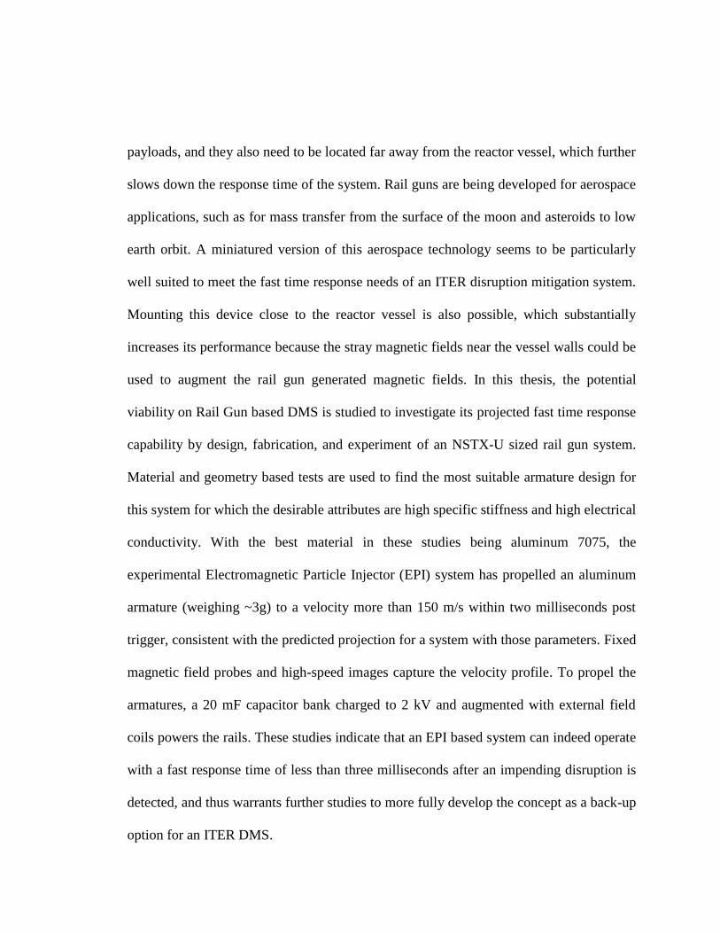
payloads, and they also need to be located far away from the reactor vessel, which further

slows down the response time of the system. Rail guns are being developed for aerospace

applications, such as for mass transfer from the surface of the moon and asteroids to low

earth orbit. A miniatured version of this aerospace technology seems to be particularly

well suited to meet the fast time response needs of an ITER disruption mitigation system.

Mounting this device close to the reactor vessel is also possible, which substantially

increases its performance because the stray magnetic fields near the vessel walls could be

used to augment the rail gun generated magnetic fields. In this thesis, the potential

viability on Rail Gun based DMS is studied to investigate its projected fast time response

capability by design, fabrication, and experiment of an NSTX-U sized rail gun system.

Material and geometry based tests are used to find the most suitable armature design for

this system for which the desirable attributes are high specific stiffness and high electrical

conductivity. With the best material in these studies being aluminum 7075, the

experimental Electromagnetic Particle Injector (EPI) system has propelled an aluminum

armature (weighing ~3g) to a velocity more than 150 m/s within two milliseconds post

trigger, consistent with the predicted projection for a system with those parameters. Fixed

magnetic field probes and high-speed images capture the velocity profile. To propel the

armatures, a 20 mF capacitor bank charged to 2 kV and augmented with external field

coils powers the rails. These studies indicate that an EPI based system can indeed operate

with a fast response time of less than three milliseconds after an impending disruption is

detected, and thus warrants further studies to more fully develop the concept as a back-up

option for an ITER DMS.

i

TABLE OF CONTENTS

List of Figures .................................................................................................................... iii

List of Tables ...................................................................................................................... v

Chapter 1. Introduction ....................................................................................................... 1

Chapter 2. Rail gun and Rail gun Applications .................................................................. 3

2.1 Rail gun ............................................................................................................... 3

2.2 Rail gun Applications ......................................................................................... 4

2.2.1 Launch of Spacecraft ...................................................................................... 4

2.2.2 Spacecraft Propulsion ..................................................................................... 5

2.2.3 Naval Gun ....................................................................................................... 6

Chapter 3. Present Disruption Mitigation System Technology .......................................... 7

3.1 Massive Gas Injection ......................................................................................... 7

3.2 Shatter Pellet Injection ...................................................................................... 11

Chapter 4. Potential Benefits of the Electromagnetic Particle Injector System ............... 13

Chapter 5. System Design ................................................................................................. 16

Chapter 6. Calculation of Velocity and Distance Parameters ........................................... 28

Chapter 7. Data Analysis .................................................................................................. 33

7.1 Comparison between Materials ......................................................................... 36

ii

7.2 External Field Augmentation ............................................................................ 38

7.3 Varying Armature Thickness ............................................................................ 43

7.4 Scaling Up for NSTX-U and ITER ................................................................... 46

Chapter 8. Conclusion ....................................................................................................... 49

Bibliography ..................................................................................................................... 51

iii

LIST OF FIGURES

Figure 2.1. Cartoon to show the operating principles of a rail gun. The electrodes

are shown in green and the armature is shown in red. I is the current through

the rails, L is the distance between, and B is the magnetic field between the

rails. ..............................................................................................................................3

Figure 3.1. (left) The isometric and cross-sectional view of the first version.

(right) The final version of the valve that includes two conductive plates to

reduce net Lorentz forces acting on the valve during operation in

environments with external magnetic fields. ...............................................................8

Figure 3.2. (left) A 10.5” chassis that houses the capacitor and other power supply

components. (right) A separate 7” chassis that houses the high voltage power

supply. ..........................................................................................................................9

Figure 3.3. The final version of one of the three MGI valves installed on NSTX-

U. A total of three valves are installed on NSTX-U. Two valves are fully

operational. ...................................................................................................................9

Figure 5.1. Rear view of the injector assembly. ................................................................17

Figure 5.2. (left) The hand-made magnetic field probes showing forty turns of

wiring at the end of a plastic screw. (right) The underside of the rail gun

assembly exposing the magnetic field probes. ...........................................................19

Figure 5.3. The main power supply assembly for the injector...........................................20

Figure 5.4. CAD model of the wiring adapter design. .......................................................21

Figure 5.5. The overall experiment setup. .........................................................................22

Figure 5.6. Basic armature design for hand calculation of required initial

deflection. ...................................................................................................................24

Figure 5.7. The armature is clamped to the base as the force transducer is jogging

down. ..........................................................................................................................26

iv

Figure 6.1. A simple RLC circuit diagram where C is the capacitor, R is the

resistor, and L is the inductor. ....................................................................................28

Figure 7.1. This figure shows the magnetic probe responses for shot 13 from

December 22nd, 2016. The minimum of each signal indicates the magnetic

field strength behind the armature as well as the time it passes by that probe. .........35

Figure 7.2. The armature is shown moving to the right with the generated plasma

cloud trailing behind. .................................................................................................37

Figure 7.3. The figure shows the magnetic field strength added to the rail gun

system by augmenting solenoids. ..............................................................................39

Figure 7.4. The magnetic field strength indicated by the probe just behind the

armature with and without the assist of the external field coils. ................................40

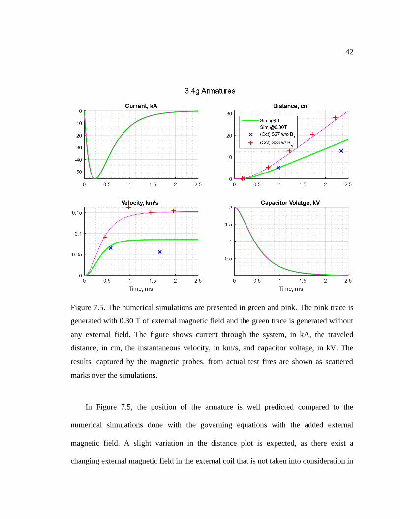
Figure 7.5. The numerical simulations are presented in green and pink. The pink

trace is generated with 0.30 T of external magnetic field and the green trace

is generated without any external field. The figure shows current of the

system, in kA, the traveled distance, in cm, the instantaneous velocity, in

km/s, and capacitor voltage, in kV. The results, captured by the magnetic

probes, from actual test fires are shown as scattered marks over the

simulations. ................................................................................................................42

Figure 7.6. Probe and high-speed data are scattered over the simulated results in

the distance and velocity plot, while the measured currents of the system are

plotted over the simulations. The data from probes are shown with a thicker

marker size than the data obtained from high-speed footages. ..................................45

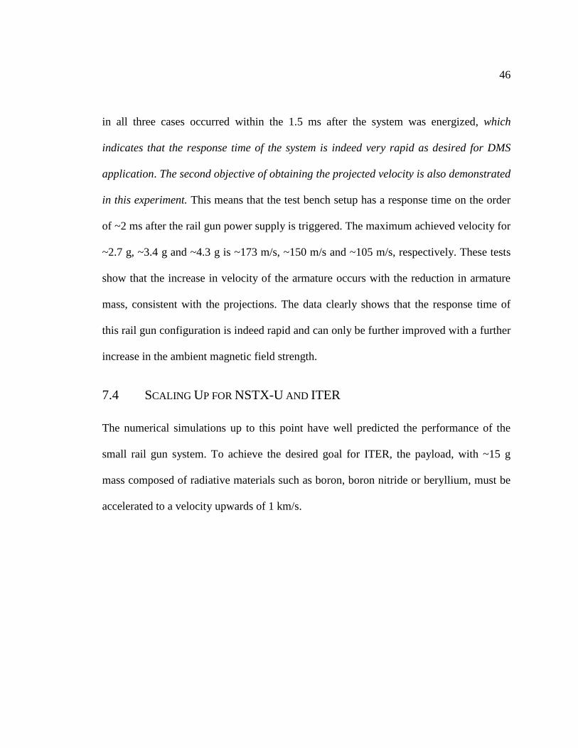
Figure 7.7. Shown are numerical simulations for accelerating the required payload

with 0 T, 2 T, 4 T ambient fields, represented as ITER A, ITER B, ITER C,

respectively. ...............................................................................................................47

v

LIST OF TABLES

Table 5.1. Results from the Intron compression test of the armatures. .............................27

Table 7.1. The calibration factor of each probe based on recorded magnetic field

strength .......................................................................................................................34

Table 7.2. The calibration factors of each probe based on the recorded magnetic

field strength ..............................................................................................................37

Table 7.3. The thickness and masses of the water-jetted armatures with tungsten

sprayed tips. ...............................................................................................................44

vi

ACKNOWLEDGEMENTS

First and foremost, I am grateful to Dr. Roger Raman, my thesis advisor, for guiding

me and providing me the opportunity to design and develop this rail gun system.

Furthermore, I would like to thank Dr. R. Raman again for helping me win two awards

from two separate AIAA competitions, which involved him listening to my presentations,

and suggesting improvements. Both awards feature the experiments done as part of this

thesis, and the design recommendations for implementing the EPI system on tokamaks.

Special thanks to Professor Thomas Jarboe for providing insights on rail gun physics

and design inputs. Many thanks to John Rogers and Johnathan Hayward for experimental

support and wealth of technical knowledge on various topics. Also, thanks to Dzung Tran

who taught me the basics in the machine shop to build all the experiments.

I could not have done it without the help and love from family (my parents, sister,

aunt, and uncle). Without their support, I would not have been able to pursue my

education so freely.

Finally, I would like to acknowledge a special someone, who has been supporting

me throughout my entire aerospace engineering endeavors in the Master’s program.

Thank you to my girlfriend for her attentive listening and input in technical writing.

This work is supported by U.S. Department of Energy contract numbers DE-

SC0006757 and DE-AC02-09CH11466.

vii

DEDICATION

to my family

Jiann Horng, Meng Hsueh, Ying Huei

to my aunt and uncle

John and Lynn

to my loving girlfriend

Jennifer

1

Chapter 1. INTRODUCTION

A major disruption can be devastating to continuous development and testing of the

International Thermonuclear Experimental Reactor (ITER). A tokamak-designed

magnetic confinement device, like ITER, that carries a large current to generate plasma

equilibrium has the potential to disrupt. Disruption occurs when the stability of the

magnetic equilibrium, which suspends the fuel away from the walls, is lost. When this

happens, the large thermal energy in the magnetic bottle is rapidly lost – this is called a

disruption. Disruption can cause severe damage to the internal vessel components;

therefore, methods for mitigating a disruption are needed.

Tokamak disruptions can be mitigated by uniformly radiating the stored thermal

energy by depositing the energy uniformly on the vessel walls, rather than locally in

small regions. At the moment, ITER has adopted two Disruption Mitigation Systems

(DMS): Massive Gas Injection (MGI) [1] and Shattered Pellet Injection (SPI) [2]. The

velocities of cryogenic shatterable pellets and the response of gas injectors depend

heavily on the sound speed in the propelling gas or the gas expansion velocity. Thus, the

response time of these methods may be insufficient for disruptions with a short warning

time [3].

In this paper, an Electromagnetic Particle Injector (EPI) is proposed as a back-up

DMS for ITER. The main advantage of an EPI is its potential to meet the short warning

time scales to rapidly quench the discharge after an impeding disruption is detected [4].

2

The EPI system is a linear rail gun, and can inject payloads such as boron, boron nitride

or beryllium into the plasma stream to quench the plasma discharge. Calculations suggest

that the system can respond within the 2-3 ms time scale, which is significantly faster

than other methods that are in use at present. To test and verify the predicted system

response time, and the achievable velocity in this short 2-3 ms time scale, a small-scale

EPI system was designed and constructed at the University of Washington for

experimental testing. Material and geometry based tests were conducted to find the most

successful armature design for this system. This EPI system has a bore cross-section of 2

cm x 2 cm and has a usable length of 1.22 m. It is driven by a capacitor-based power

supply system with a total capacitance of 20 mF at a maximum operating voltage of

2 kV. External electromagnets are also added to the system to validate the predicted

performance improvement due to ambient magnetic field augmentation.

3

Chapter 2. RAIL GUN AND RAIL GUN APPLICATIONS

In this chapter, the theory behind a functioning electromagnetic rail gun is explained, and

a number of rail gun applications are described.

2.1 RAIL GUN

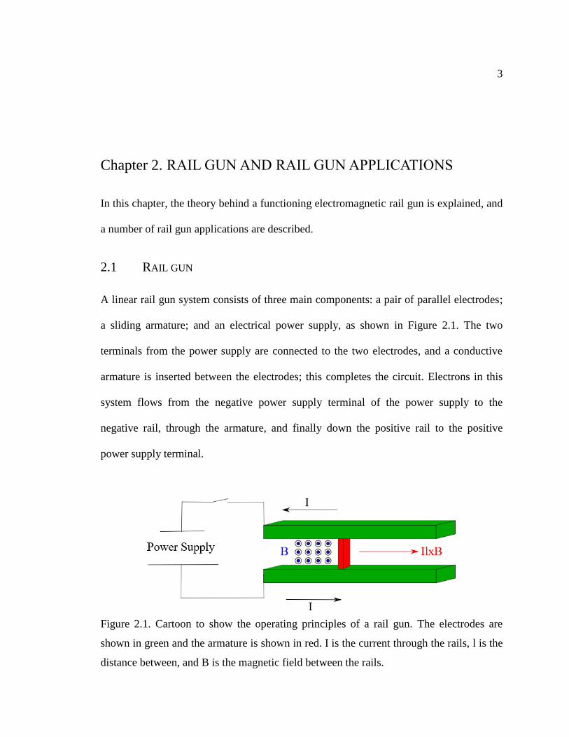
A linear rail gun system consists of three main components: a pair of parallel electrodes;

a sliding armature; and an electrical power supply, as shown in Figure 2.1. The two

terminals from the power supply are connected to the two electrodes, and a conductive

armature is inserted between the electrodes; this completes the circuit. Electrons in this

system flows from the negative power supply terminal of the power supply to the

negative rail, through the armature, and finally down the positive rail to the positive

power supply terminal.

Figure 2.1. Cartoon to show the operating principles of a rail gun. The electrodes are

shown in green and the armature is shown in red. I is the current through the rails, l is the

distance between, and B is the magnetic field between the rails.

4

From Ampere’s law, any electrical current flowing through a conductive wire will

generate a magnetic field around that wire. In the case of a rail gun, the current in the

rails generates a magnetic field between the rails. The current through the armature in

combination with the magnetic field B between the rails produces a Lorentz force, which

accelerates the projectile down the linear rail gun assembly. The Lorentz force law

provides the force acting on the armature:

Farm⃑⃑ ⃑⃑ ⃑⃑ ⃑⃑ =I 𝑙× B⃑⃑ (2.1)

where I is the current through the armature, l is the gap distance between the rails and B⃑⃑

is the magnetic field seen by the armature.

2.2 RAIL GUN APPLICATIONS

Rail gun technology has a great number of applications primarily in aerospace and

military. A few examples are shown and discussed in the following subsections.

2.2.1 Launch of Spacecraft

Liquid fuels and solid propellants have dominated spaceflight technologies for be the past

half century. One of the main advantages of this technology is that the rocket gains speed

slowly from the launch pad. This allows for fragile cargos or astronauts to hitch along for

the ride. It also allows for minimal aerodynamic and aerothermal loads due to its modest

velocities. However, there is also a large trade-off, as the final mass that reaches orbit

5

tends to be a small fraction of the initial total mass. The cost per kilogram of payload sent

to near-Earth orbit is >$20,000 [5]. A paper by McNab describes the uses of propulsion

options for outer space deliveries, which includes electromagnetic rail guns;

electromagnetic coil guns; electrothermal-chemical guns; light gas guns; RAM

accelerator; blast wave accelerator; slingatron; and lasers [5]. In this paper by McNab, the

rail gun system was chosen as the system of choice for its potential for reducing the cost

for near-Earth orbit delivery from >$20,000 to ~$500 (per kilogram).

2.2.2 Spacecraft Propulsion

Due to the higher specific impulse and lower system mass, plasma thrusters are favored

over chemical counterparts for missions such as station-keeping and orbital raising of

spacecraft [6]. Plasma thrusters are especially applicable if the spacecraft already has a

surplus of electricity from solar energy. A Pulsed Plasma Thruster (PPT) is similar in

concept to a rail gun. The power supply generates an arc of electricity that is needed to

generate a cloud of plasma resulting from the ablation of the fuel (usually PTFE). The

plasmoid completes the circuit and is propelled down the barrel due to Lorentz force.

Because of the simplicity in its design, this propulsion system has lower cost compared to

other plasma thrusters. Furthermore, PTT was one of the first forms of electric propulsion

to be flown in space, (equipped on Zond 2). PPT is also considered for planetary and

deep space explorations as described in [7], as it is able provide the high exhaust speed

over a long duration of time.

6

2.2.3 Naval Gun

Installing an electromagnetic rail gun on a destroyer seems ideal as the only type of

energy required to power a rail gun system is electricity. Next generation (Zumwalt-

class) destroyers are able to generate an excess ~58 MW of reserve power from their

engines [8]. With the abundant energy source, these destroyers can be upgraded with new

weapon systems such as a rail gun. In [9], McFarland describes a rail gun system that

makes it possible to fire high-energy projectiles between ranges of 300-500 km at a rate

of 12 rounds per minute. These projectiles are designed to have a launch mass of 21.9 kg

and a flight mass of 16.4 kg; it would travel out of the barrel at a speed of 2 km/s. With

an assumed gun efficiency of 50%, ~35 MW of power is required during the firing

operations. Furthermore, by fitting a rail gun system to the destroyer, it could eliminate a

total of 9,000 MJ of chemical energy stored in the form of conventional ammunition [9].

This ensures a large increase in ship survivability as electromagnetic gun rounds lack

chemical propellant.

7

Chapter 3. PRESENT DISRUPTION MITIGATION SYSTEM

TECHNOLOGY

This chapter describes the current systems that are considered by ITER for disruption

mitigation and their limitations.

3.1 MASSIVE GAS INJECTION

As described in the introduction, MGI is one of the adopted DMS technologies by ITER

and by many tokamaks. MGI is a well-establish technology for mitigating disruptions in

several tokamaks such as DIII-D [10] and JET [11]. MGI works, as the name suggests, by

injecting a large volume of radiative gas to rapidly cool the plasma inside the tokamak.

During the initial part of this thesis, a number of MGI valves were designed and

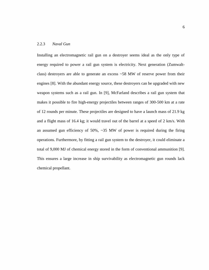
two are shown in Figure 3.1. Figure 3.1 shows the initial and the final versions of the

valve that were designed for NSTX-U. The valve operates by repelling a conductive plate

due to eddy currents induced on it by a rapidly changing magnetic field produced by the

solenoid that sits below the conductive plate in the solenoid chamber. This causes the

plunger to open and allow the gas in the primary plenum to flow into the tokamak vessel.

The primary plenum holds the pressurized radiative gas while the gas in the secondary

plenum is lower and adjusted to maintain just enough over pressure to make the lower O-

ring seal. The final version of the MGI valve has dual conductive plates to reduce the

total torque acting on the piston during operations in an external magnetic field.

8

Figure 3.1. (left) The isometric and cross-sectional view of the first version. (right) The

final version of the valve that includes two conductive plates to reduce net Lorentz forces

acting on the valve during operation in environments with external magnetic fields. The

dual conductive plate concept is an Oak Ridge National Laboratory innovation that was

adopted for the NSTX-U valve design.

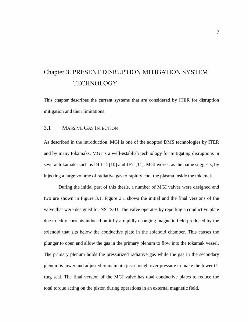
The power supply for each valve utilizes a 550 μF capacitor that can be charged up

to 1.5 kV, shown in Figure 3.2. The typical operating voltage is 900 V. In testing, each

valve is capable of injecting over 27 Pa · m3 of the required radiative gas, which can be

neon, argon, or a mixture of helium with these gases [12].

9

Figure 3.2. (left) A 10.5” high chassis that houses the capacitor and other power supply

components. (right) A separate 7” high chassis that houses the high voltage power

supply.

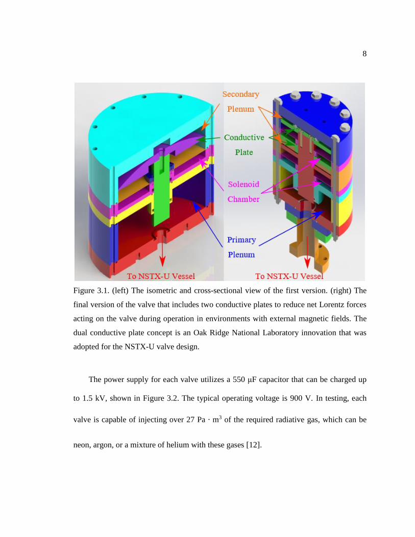
Figure 3.3. The final version of one of the three MGI valves installed on NSTX-U. A

total of three valves are installed on NSTX-U. Two valves are fully operational.

10

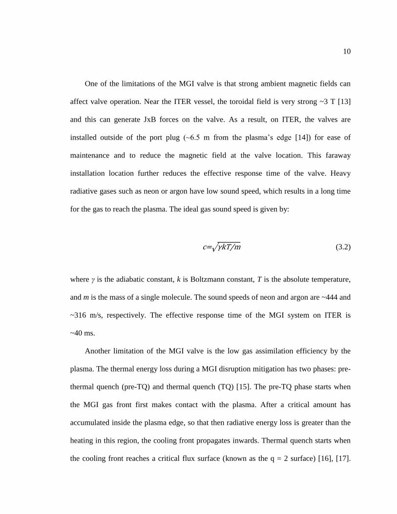
One of the limitations of the MGI valve is that strong ambient magnetic fields can

affect valve operation. Near the ITER vessel, the toroidal field is very strong ~3 T [13]

and this can generate JxB forces on the valve. As a result, on ITER, the valves are

installed outside of the port plug (~6.5 m from the plasma’s edge [14]) for ease of

maintenance and to reduce the magnetic field at the valve location. This faraway

installation location further reduces the effective response time of the valve. Heavy

radiative gases such as neon or argon have low sound speed, which results in a long time

for the gas to reach the plasma. The ideal gas sound speed is given by:

c=√γkT/m (3.2)

where γ is the adiabatic constant, k is Boltzmann constant, T is the absolute temperature,

and m is the mass of a single molecule. The sound speeds of neon and argon are ~444 and

~316 m/s, respectively. The effective response time of the MGI system on ITER is

~40 ms.

Another limitation of the MGI valve is the low gas assimilation efficiency by the

plasma. The thermal energy loss during a MGI disruption mitigation has two phases: pre-

thermal quench (pre-TQ) and thermal quench (TQ) [15]. The pre-TQ phase starts when

the MGI gas front first makes contact with the plasma. After a critical amount has

accumulated inside the plasma edge, so that then radiative energy loss is greater than the

heating in this region, the cooling front propagates inwards. Thermal quench starts when

the cooling front reaches a critical flux surface (known as the q = 2 surface) [16], [17].

11

Unlike current devices, the plasma edge of ITER has much higher energy content and the

volume of the plasma is much larger (~30 times DIII-D and ~7 times JET). The injected

gas must first penetrate an energetic scrape-off layer before it can be assimilated by the

plasma [4]. Consequently, the machine size scaling for MGI becomes less favorable as

the machine size is increased. However, because of the simplicity of the MGI concept,

many current tokamaks will continue to use this technology for machine protection and it

may even be used on future tokamaks as back-up system to mitigate disruptions that have

sufficient warning time.

3.2 SHATTER PELLET INJECTION

In a Shattered Pellet Injector (SPI) the MGI valve is used to propel a cylindrical

cryogenic pellet (using the injection gas as in a gas gun) as the radiative payload. These

pellets are made of frozen neon or argon. Injection of an intact salvo could damage the

inner wall upon impact. Therefore, the pellet is shattered using a metal plate or forced

through a tight bend in the guide tube before entering the vessel. The ablation plate

shattering method allows for a large increase in surface area of the frozen impurities [18],

[19]. The sub-millimeter size shards then enter the plasma.

One advantage of this technology is that solid impurities are injected directly into the

plasma. However, the pellet can only achieve a maximum velocity of ~300-400 m/s [14]

and the velocity of the shattered fragments is much less. Therefore, the system response

time is still slow.

12

Due to the mechanical nature of the two methods (MGI and SPI) and the use of

cryogenic and plastics, they cannot be placed close to the ITER vessel, where strong

magnetic field of ~3 T and a harsh radiation environment can hinder their operation. The

EPI system described in this paper is not hindered by its exposure to the strong magnetic

fields; it actually takes advantage of this. The EPI system can be placed close to the

vessel walls since there are no mechanical-moving parts and plastics. It also has the

potential benefit of rapid response time (in the order of ~2-3 ms) after a command is sent

to trigger the system. These benefits are described in Chapter 4.

13

Chapter 4. POTENTIAL BENEFITS OF THE

ELECTROMAGNETIC PARTICLE INJECTOR

SYSTEM

The electromagnetic particle injector, based on a simple rail gun concept, has the

potential to respond to disruptions within a few milliseconds. Possible ways to increase

the performance of a linear rail gun injector are discussed.

From Eq. (2.1), one can increase the performance of the rail gun by increasing the

current going through the system. This is generally avoided, as increasing current in the

system gives rise to resistive heating and plasma arc generation. Both properties reduce

the efficiency and longevity of the system. If the system is continuously operated at high

currents, erosions will eventually deteriorate the surface of the rails to the point where the

cross section of the bore is uneven and injector operation will become irreproducible. It

can also compromise its goal as the assembly of payload and armature may get trapped

and it may be difficult to dislodge them when injection is required, therefore rail guns are

not meant for high duty cycle applications. In the case where a plasma arc is generated,

the current going through the armature will diminish, as this arc will continue down the

barrel and travel ahead of the armature while carrying a portion of the injected current.

Thus, it is very desirable to find ways to improve the gun performance without increasing

the gun current.

14

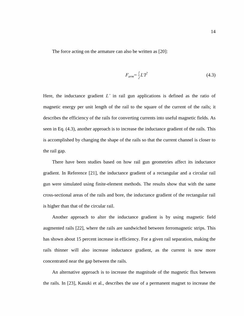
The force acting on the armature can also be written as [20]:

Farm=1

2L'I2 (4.3)

Here, the inductance gradient L’ in rail gun applications is defined as the ratio of

magnetic energy per unit length of the rail to the square of the current of the rails; it

describes the efficiency of the rails for converting currents into useful magnetic fields. As

seen in Eq. (4.3), another approach is to increase the inductance gradient of the rails. This

is accomplished by changing the shape of the rails so that the current channel is closer to

the rail gap.

There have been studies based on how rail gun geometries affect its inductance

gradient. In Reference [21], the inductance gradient of a rectangular and a circular rail

gun were simulated using finite-element methods. The results show that with the same

cross-sectional areas of the rails and bore, the inductance gradient of the rectangular rail

is higher than that of the circular rail.

Another approach to alter the inductance gradient is by using magnetic field

augmented rails [22], where the rails are sandwiched between ferromagnetic strips. This

has shown about 15 percent increase in efficiency. For a given rail separation, making the

rails thinner will also increase inductance gradient, as the current is now more

concentrated near the gap between the rails.

An alternative approach is to increase the magnitude of the magnetic flux between

the rails. In [23], Kasuki et al., describes the use of a permanent magnet to increase the

15

rail gun performance. If the rail gun is augmented using an external magnetic field, the

external magnetic field, Bext, needs to be factored into Eq. (4.3) and the total force acting

on the armature is expressed as:

Farm=md

2z

dt2=

1

2L'I2+IBexth (4.4)

Here m is the mass of the armature, z is the position of the armature, t is time, and h is the

separation gap between the rails. The additional contribution from the external magnetic

field reduces the required current from the power supply for an otherwise similar velocity

profile. However, mounting permanent magnets or magnetic coils onto the rail gun can

complicate the geometries and the setup. Fortunately, for DMS applications, this is a

major advantage as in a large tokamak environment such as ITER, the high magnetic

fields near the vessel walls are naturally present, and this could be used to boost the rail-

generated magnetic fields. This large magnetic field is usually a problem for most

systems that involve mechanical moving components, however, there are no moving

parts in a rail gun (except the armature itself, which benefits from this external field).

With proper alignment of the rails with this external field, this additional magnetic field

could be used to improve the performance of a rail gun system as described later. In

Chapter 7, it is shown that this external field dramatically reduces the required capacitor

bank size and required current while maintaining otherwise similar acceleration force,

and is particularly helpful for the application of a rail gun as a Disruption Mitigation

System (DMS) in ITER, as will be shown later.

16

Chapter 5. SYSTEM DESIGN

The design goals for the University of Washington rail gun test facility call for a

repeatable and reliable platform for future improvements and installations.

For the system described in this thesis, the rails are made of extruded 360 free

machining brass, as this material is highly machinable and affordable. Since the first, and

the most important, objective was to verify the system response time, this was deemed to

be a good low cost method to test the concept. The original designed dimensions of the

rails were 20.0 mm x 20.0 mm by 1.52 m long. However, after surfacing the brass bar

using a conventional mill, on one side, to the 20.0 mm thickness, it was noted that the bar

curved due to the loss of surface tension. The tensioned surfaces are introduced during

the manufacturing phase of the bar due to the difference in cooling rate throughout the

bar thickness. This phenomenon causes the bar to bend more and more in the opposite

direction of the machining face as material is removed. This required a slight alteration to

the rail design. In order to minimize this effect such that the rails can stay relatively true

and straight during assembly and testing, the cross section of the rails was limited to 20.0

mm high x 25.4 mm wide. This ensured that the bars would not bend in or out of the path

of the armature as it slides down the barrel.

After the initial batch of tests, the rails had a great amount of surface erosion caused

by plasma arcs and resistive heating during test fires. These brass rails were deemed too

17

soft at its surfaces. To increase surface hardness, a few layers of pure tungsten were

plasma sprayed onto the inner surfaces of the rail. The tungsten layer allows the surface

hardness to increase from Rockwell HRB 35 (~HRA 29) to HRA 50, which means higher

sliding wear and erosion resistance.

The as-sprayed surface finish from the coating company was not touched and was

used to run several test shots. However, it was found that the surface finish of the

coatings was too rough and it was creating too much friction at the contacts. These rails

were re-serviced using diamond files to smooth out the roughness.

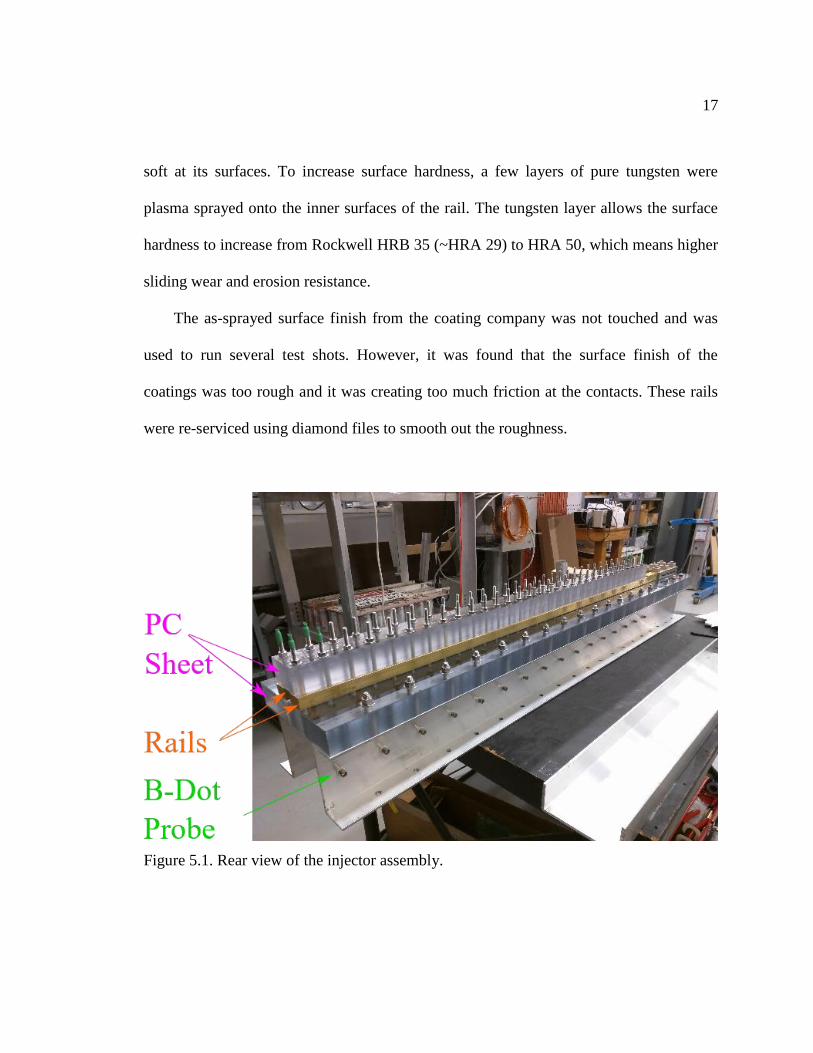
Figure 5.1. Rear view of the injector assembly.

18

As shown in Figure 5.1, the machined rails are clamped between two sheets of 38.1

mm, “thick”, polycarbonate (PC) sheets. To prevent the surfaces of the polycarbonates

from deteriorating over multiple shots, there exists a 1.56 mm, “thin”, polycarbonate

sheet between the rails and the “thick” polycarbonate plates. The lower “thick” plate is

then bolted to two rows of aluminum C-channels. The “thick” polycarbonate plates are

chosen as they allow for clear transparency through the cross section of the gun. This

transparency characteristic of the polycarbonate sheets permits a slow-motion camera to

be deployed to take pictures of the rail gun during operation using a top-down view.

The slow-motion camera deployed is a Vision Research Phantom v12.1, which has

the ability of obtaining 16,000 frames per second at 1,280 x 232 pixels. It is used to

observe the armature through the polycarbonate sheets. The primary use is to diagnose

areas of problems such as arc generation and armature deformation during acceleration.

Its secondary role is to track the location of the armature with respect to time, which can

then be translated to the armatures’ velocity and acceleration.

19

Figure 5.2. (left) The hand-made magnetic field probes showing forty turns of wiring at

the end of a plastic screw. (right) The underside of the rail gun assembly exposing the

magnetic field probes.

As shown in Figure 5.2, magnetic probes are also installed beneath the rail gun.

These allow us to track the position of the armature during its acceleration, as well as

inform us of the magnetic field strength experienced by the armature. The probes are

spaced 76.2 mm apart and are evenly distributed throughout the injector. A magnetic

probe (or B-dot probe) works by measuring the voltage due to a change in the magnetic

flux through the enclosed area of the windings. The details of the probe operations and

calibrations are described in Chapter 7. These probes, combined with the slow-motion

footage, enable us to determine the position of the armature with respect to time.

20

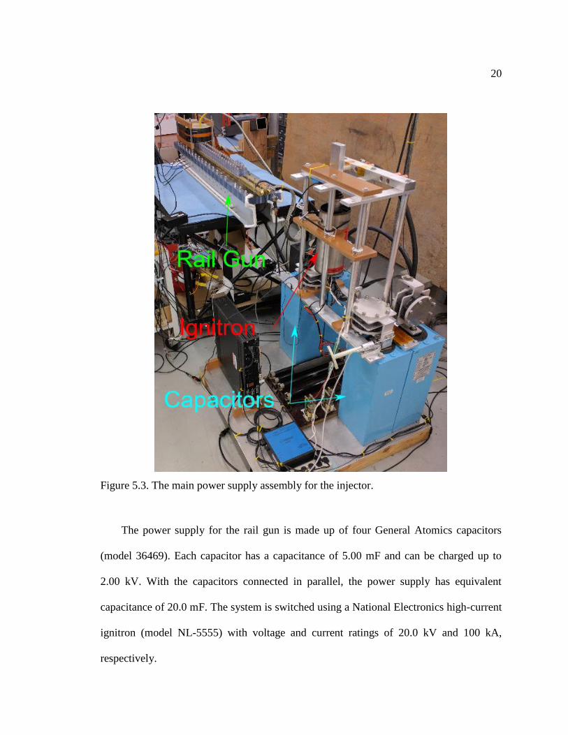
Figure 5.3. The main power supply assembly for the injector.

The power supply for the rail gun is made up of four General Atomics capacitors

(model 36469). Each capacitor has a capacitance of 5.00 mF and can be charged up to

2.00 kV. With the capacitors connected in parallel, the power supply has equivalent

capacitance of 20.0 mF. The system is switched using a National Electronics high-current

ignitron (model NL-5555) with voltage and current ratings of 20.0 kV and 100 kA,

respectively.

21

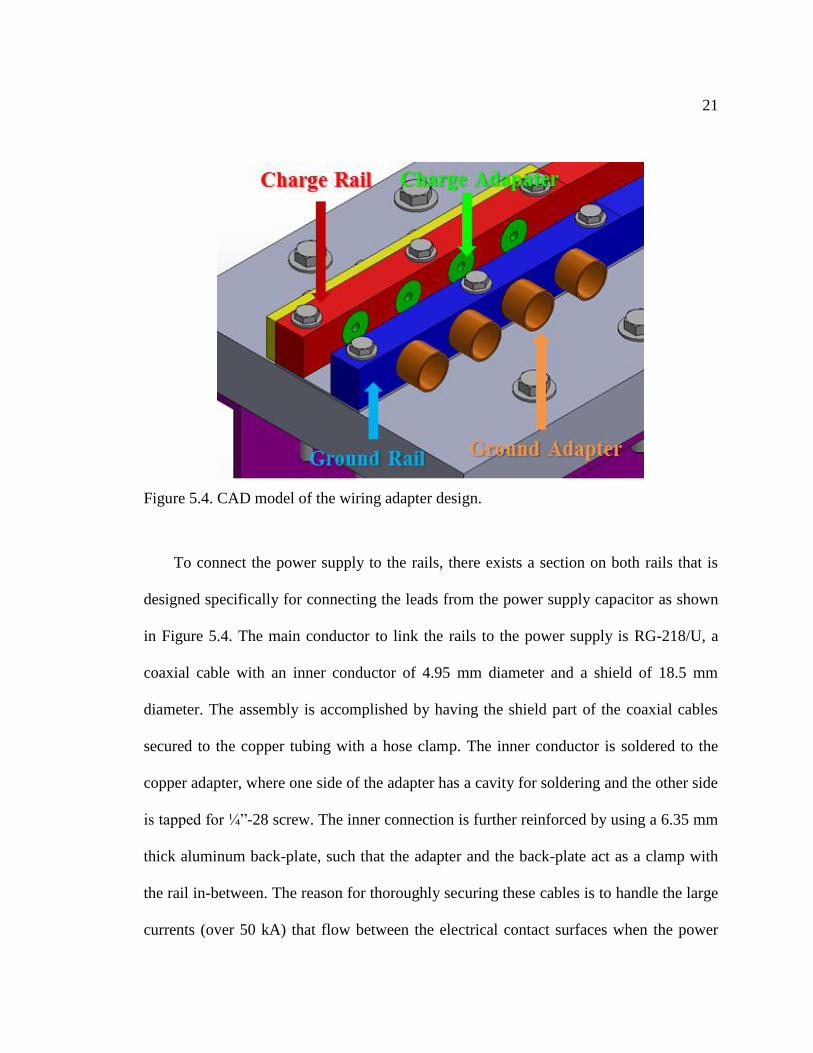
Figure 5.4. CAD model of the wiring adapter design.

To connect the power supply to the rails, there exists a section on both rails that is

designed specifically for connecting the leads from the power supply capacitor as shown

in Figure 5.4. The main conductor to link the rails to the power supply is RG-218/U, a

coaxial cable with an inner conductor of 4.95 mm diameter and a shield of 18.5 mm

diameter. The assembly is accomplished by having the shield part of the coaxial cables

secured to the copper tubing with a hose clamp. The inner conductor is soldered to the

copper adapter, where one side of the adapter has a cavity for soldering and the other side

is tapped for ¼”-28 screw. The inner connection is further reinforced by using a 6.35 mm

thick aluminum back-plate, such that the adapter and the back-plate act as a clamp with

the rail in-between. The reason for thoroughly securing these cables is to handle the large

currents (over 50 kA) that flow between the electrical contact surfaces when the power

22

supply is energized. Also, due to the thickness of this cable, the stiffness of the RG-218/U

cable also needs to be considered.

The power supply for the external field coils consists of two capacitors, fabricated by

CSI, each with a capacitance of 5 mF and a maximum voltage rating of 2 kV. These two

capacitors are connected in parallel and give the power supply an equivalent of 10 mF

capacitance. The capacitors are connected to the two coils that are positioned on top of

the rails via a PRX silicon controlled rectifier (model LS411860) with voltage and

average current ratings of 1.80 kV and 600 A, respectively. The two coils are connected

in series. For this application, the power supply that was built for the MGI valve (Figure

3.2) was modified to be used with the much larger 10 mF capacitor bank.

Figure 5.5. The overall experiment setup.

23

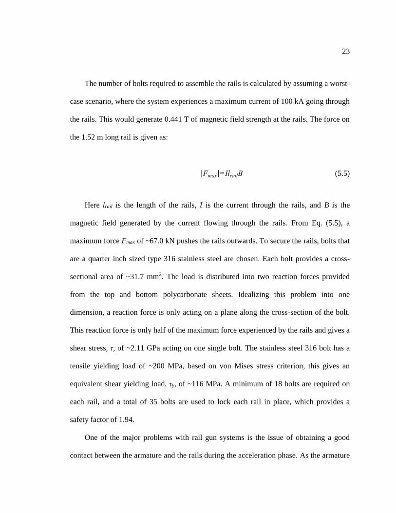
The number of bolts required to assemble the rails is calculated by assuming a worst-

case scenario, where the system experiences a maximum current of 100 kA going through

the rails. This would generate 0.441 T of magnetic field strength at the rails. The force on

the 1.52 m long rail is given as:

|Fmax|=IlrailB (5.5)

Here lrail is the length of the rails, I is the current through the rails, and B is the

magnetic field generated by the current flowing through the rails. From Eq. (5.5), a

maximum force Fmax of ~67.0 kN pushes the rails outwards. To secure the rails, bolts that

are a quarter inch sized type 316 stainless steel are chosen. Each bolt provides a cross-

sectional area of ~31.7 mm2. The load is distributed into two reaction forces provided

from the top and bottom polycarbonate sheets. Idealizing this problem into one

dimension, a reaction force is only acting on a plane along the cross-section of the bolt.

This reaction force is only half of the maximum force experienced by the rails and gives a

shear stress, τ, of ~2.11 GPa acting on one single bolt. The stainless steel 316 bolt has a

tensile yielding load of ~200 MPa, based on von Mises stress criterion, this gives an

equivalent shear yielding load, τy, of ~116 MPa. A minimum of 18 bolts are required on

each rail, and a total of 35 bolts are used to lock each rail in place, which provides a

safety factor of 1.94.

One of the major problems with rail gun systems is the issue of obtaining a good

contact between the armature and the rails during the acceleration phase. As the armature

24

is accelerated due to Lorentz force, the edges, where contacts are made, experience large

electrical currents and friction with the electrodes. The effects of high current and wall

friction cause erosion and good current contact can be lost [24], [25]. Not only does this

mean that the interface between the armature and the rails are significantly compromised,

but also that the surfaces of the rails are damaged along the barrel. This is the main

reason why rail guns have significant erosion and performance issues. In this paper, the

proposed armature designs are given spring-like properties and tested with a variation of

material and material thicknesses.

The design of the armature heavily depends on three parameters: elasticity (spring-

like) properties, electrical conductivity and weight limits. The most ideal material would

have high stiffness, low mass and good electrical conductivity. Four alloys are described

in this paper: aluminum 7075-T6, aluminum 6061-T6, brass 464 and copper 101.

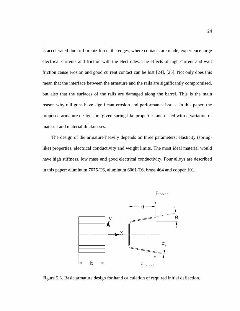
Figure 5.6. Basic armature design for hand calculation of required initial deflection.

25

As shown in Figure 5.6, this basic armature design is symmetric about its midplane,

so the calculation for its initial angle of deflection θ is simplified to a fixed cantilever

beam problem with a contact force acting at the end of the beam. The thickness of the

armature h is much smaller than its length d, so Euler-Bernoulli beam theory is used for

this approximation. The theory describes the bending moment of a beam as:

M= -E×I×d

2w

dx2 (5.6)

where E is the Young’s modulus (Pa) of a given material, I is the second area moment

(m4) of the armature, and w is the downward deflection (m) of the beam at some position

x. Based on Eq. (5.6) and cantilever beam boundary conditions, the maximum stress,

σmax, due to the contact load occurs at the fixed end.

σmax=6×d×Fcontact

b×h2 (5.7)

Here b, h, and d are the width, thickness, and length of the armature, respectively,

and Fcontact is the force acting at the free end of the armature. The maximum stress in the

armature should not exceed a stress level higher than the tensile yielding stress.

Otherwise, the spring will undergo plastic deformation and will not result in an elastic

behavior. By integrating Eq. (5.6), the initial angle of deflection, θ0, required is described

as:

26

θ0=6×d2×Fcontact

b×h3×E (5.8)

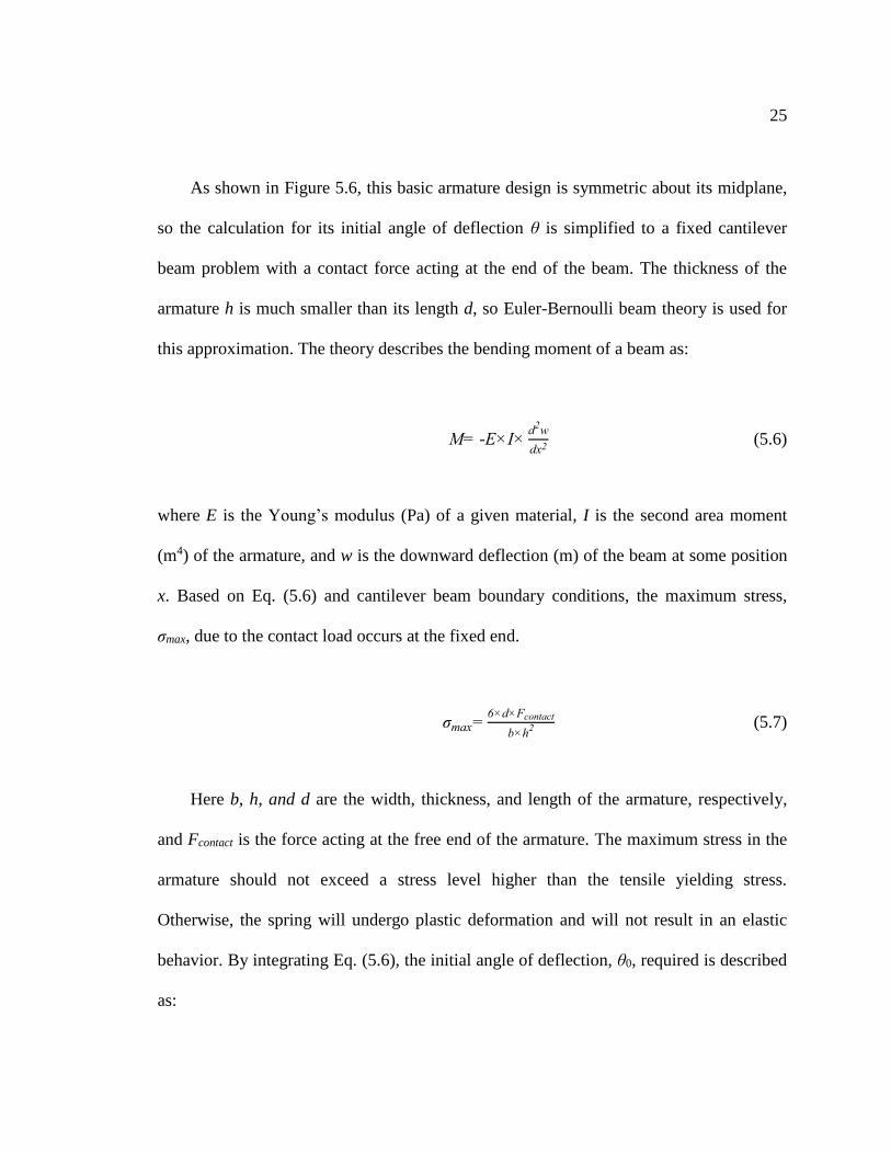
Several armatures were made with thicknesses varying from ~1.02 mm to ~2.03 mm.

They were further tested using an Intron loading frame (5585H) to find their force to

deflection relationships. The test setup is shown in Figure 5.7.

Figure 5.7. The armature is clamped to the base as the force transducer is jogging down.

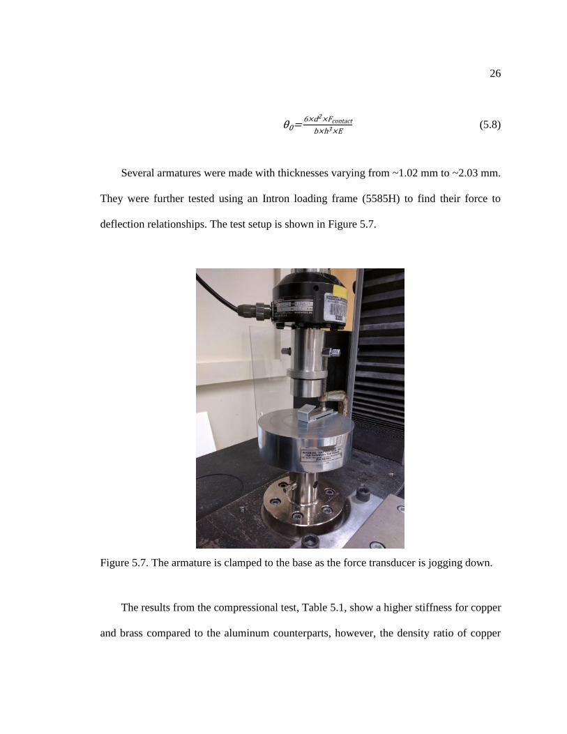
The results from the compressional test, Table 5.1, show a higher stiffness for copper

and brass compared to the aluminum counterparts, however, the density ratio of copper

27

and brass to aluminum is 3.30 and 3.11, respectively. The aluminum samples show a

higher specific stiffness and so is the ideal material for the armature.

Table 5.1. Results from the Intron compression test of the armatures.

Material Thickness,

mm

Sample 1,

N/m

Sample 2,

N/m

Sample 3,

N/m

Average,

N/m

Density,

g/cm3

Al 6061-

T6

1.59 25.9 26.6 27.9 26.8 2.70

Al 6061-

T6

2.03 94.9 83.7 93.0 90.5 2.70

Al 7075-

T6

1.27 19.7 19.9 20.6 20.1 2.81

Cu 101-

H00

2.03 149 144 141 145 8.94

Brass

464-H01

1.59 47.0 47.6 50.1 48.2 8.41

The design of the payload is also an important task, as the ideal design should

restrain the armature from tilting as it travels down the barrel due to uneven drags. This

means the armature must maintain good electrical contact throughout the acceleration

phase, as well as constrain the armature from its tendency to rotate due to uneven friction.

The uneven loadings can cause severe deformations to the armature. The deformations

can cause difficulties in separating the armature from its payload due to the unpredictable

geometry change. This was not a primary objective of this thesis and is not discussed in

here.

28

Chapter 6. CALCULATION OF VELOCITY AND DISTANCE

PARAMETERS

The rail gun performance is simulated by simultaneously solving the equation of motion

Eq. (4.4) that is reproduced here for convenience, and the electrical circuit equation

shown below as Eq. (6.1).

Farm=md2z

dt2=

1

2L'I2+IBexth (4.4)

Here m is the mass of the armature, z is the position of the armature, L’ is the inductance

gradient (Henrys/meter), which is a constant for our case, I is the current through the

circuit, Be is the external magnetic field, and h is the gap width between the rails.

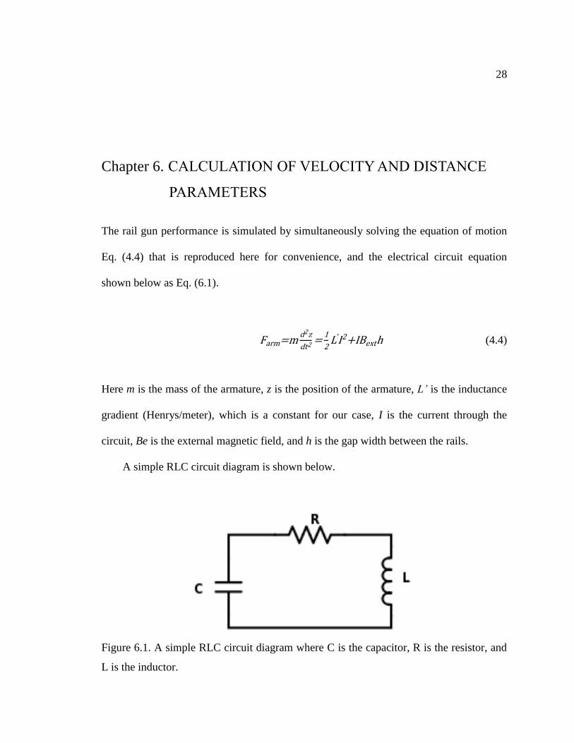
A simple RLC circuit diagram is shown below.

Figure 6.1. A simple RLC circuit diagram where C is the capacitor, R is the resistor, and

L is the inductor.

29

From Kirchhoff’s voltage law, the summation of the voltage around any closed loop is

zero. The RLC circuit equation is given as:

∑𝑉 = 𝑉𝑅 + 𝑉𝐿 + 𝑉𝐶 =𝐼𝑅 +𝑑𝐿𝐼

𝑑𝑡+ 𝑉𝐶 =𝐼𝑅 + 𝐿

𝑑𝐼

𝑑𝑡+ 𝐼

𝑑𝐿

𝑑𝑡+ 𝑉𝐶 =0 (6.1)

where VR, VL, and VC are the voltage across the resistor, the inductor, and the capacitor,

respectively. I is the current going through the circuit, R is the resistance of the circuit,

and L is the inductance of the system.

The voltage across the capacitor is given as:

𝑉𝐶 = 1

𝐶∫ 𝐼 𝑑𝑡 (6.2)

C is the capacitance of the capacitor. Differentiating both sides of Eq. (6.2) gives:

𝑑𝑉𝐶

𝑑𝑡 =

𝐼

𝐶 (6.3)

In a linear rail gun, the total inductance is the sum of external inductance, Lext,

(inductances of the cables, etc.…), and inductance based on the inductance gradient of

the rails and position of the armature, z. The total inductance is defined as:

L=Lext+L'×z (6.4)

30

The inductance gradient of a linear rail gun that utilizes rectangular rail cross-sections

can be closely estimated using the following formula [26]:

L'=106

0.5986b

s+0.9683

b

s+2g+4.3157

1

ln(4(s+g)

g )-0.7831

(6.5)

where g, s, and b are the width, separation, and the thickness of the rail, respectively.

With the inductance gradient known, the change in inductance with respect to time can be

found using the following:

dL

dt=

dL

dz

dz

dt=L've (6.6)

To simulate the rail gun performance, the ode45 function in MATLAB R2015a is

used to perform the numerical analysis. This function utilizes the explicit Runge-Kutta

formula, which has a local truncation error on the order of 5th and a global error on the

order of 4th [27]. For this function to work, we must reduce Eq. (4.4) and (6.1) to first

order differential equations. This can be achieved by assuming a state vector of four

variables as the following:

�⃗�= [

Vc

I

z

ve

] (6.7)

31

where Vc is the voltage of the capacitor, I is the current through the system, z is the

position of the armature, and ve is the velocity of the armature. Taking the derivative of

each term in Eq. (6.7):

dX⃗⃑⃑

dt=

[

dVc

dt

dI

dt

dz

dt=ve

d𝑣𝑒

dt=ae]

(6.8)

where ae is the acceleration experienced by the armature. Now, using the equations Eq.

(4.4), (6.1), (6.3), and (6.6).

dX⃗⃑⃑

dt=

[

dVc

dt=

I

C

dI

dt=

-I

C − 𝐼𝑅 − L'Ive

L

dz

dt=ve

dve

dt=

1

2L'I2 + IBeh

m ]

(6.9)

Now we have four first order differential equations with four unknowns. The initial

conditions are:

X0⃑⃑⃑⃑⃗= [

V0

I0

z0

ve,0

] = [

2000

0

0

0

] (6.10)

32

where V0 is the initial voltage on the capacitor, I0 is the initial current through the system,

z0 is the initial displacement of the armature, and ve,0 is the initial velocity of the

armature. The solution to these equations allows one to calculate the theoretical velocity

and distance parameters as a function of time as the capacitor bank energy is depleted.

These are discussed in Chapter 7.

33

Chapter 7. DATA ANALYSIS

The custom-made magnetic field sensors are calibrated individually using a large

rectangular flux loop with well-known dimensions and windings. A time rate of change

of magnetic field inside a loop will induce a voltage on the loop so as to oppose the

changing magnetic flux inside the loop. From Faraday’s Law, the voltage produced in a

coil due to the change of magnetic flux is given as:

Vcoil=-nΔ(B×A)

Δt (7.1)

where n represents the number of windings, B represents the magnetic field that exist

within the coil, A represents the enclosed area of the coil, and t represents time. This

signal is processed through a passive integrator, and the output voltage becomes:

Vout = -1

R×C∫ Vindt=

-1

R×C∫ n×A×

dB

dtdt =

-n×B×A

R×C (7.2)

Here, R and C, represents the resistance and the capacitance of the integrator circuit,

respectively. The RC time constant is typically chosen to be ten times the signal duration.

But increasing the RC time too much reduces the measurable voltage to a low level. In

this case, a RC time constant of 10 ms was used. The slight droop in the measured signal

is because the RC time constant is not long enough, but this is close enough for our

34

purposes. Manipulating the equation above, the magnetic field strength is given by the

voltage output of the flux loop as:

B=−Vout×R×C

n×A (7.3)

This magnetic field strength is computed for each calibration test shot, during which

the rails are shorted at the ends. The shorted rails form a closed loop such that all the

magnetic field probes are experiencing the same magnetic field strength during a

calibration test. The calibrated constants that are used to covert the recorded voltage

outputs, of the custom-made magnetic field probes, to magnetic field strengths are

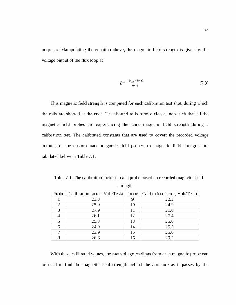
tabulated below in Table 7.1.

Table 7.1. The calibration factor of each probe based on recorded magnetic field

strength

Probe Calibration factor, Volt/Tesla Probe Calibration factor, Volt/Tesla

1 23.3 9 22.3

2 25.9 10 24.9

3 27.9 11 21.6

4 26.1 12 27.4

5 25.3 13 25.0

6 24.9 14 25.5

7 23.9 15 25.0

8 26.6 16 29.2

With these calibrated values, the raw voltage readings from each magnetic probe can

be used to find the magnetic field strength behind the armature as it passes by the

35

magnetic probe. Beyond the role of measuring the strength of the magnetic field, the

magnetic probes are also used to determine the time when the armature passes by the

probes. With known positions of these probes and recorded time stamps, the

instantaneous velocities can be found. An example of magnetic probe traces is illustrated

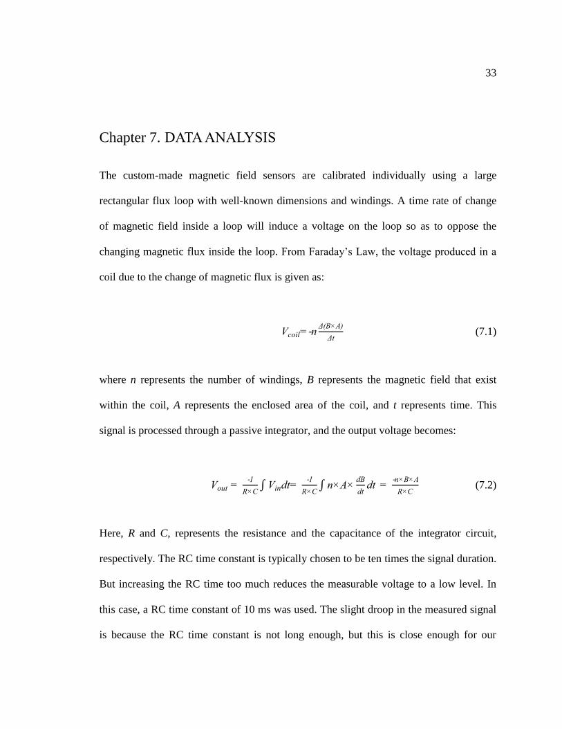
in Figure 7.1.

Figure 7.1. This figure shows the magnetic probe responses for shot 13 from December

22nd, 2016. The minimum of each signal indicates the magnetic field strength behind the

armature as well as the time it passes by that probe.

36

Figure 7.1 is generated by accelerating a ~3 g armature with the power supply

charged to 2 kV with the augmented coils. The augmentation of the external coils is

described in section 7.2. The local minimum of each trace shows the time armature

passes by a given probe. The effect of the external field coils is discussed in the latter

portion of this thesis. The magnitude of the probe signals is decreasing with time because

the current through the rails is decreasing with time.

7.1 COMPARISON BETWEEN MATERIALS

The initial test shots were conducted with the capacitors charged to 2 kV. The surface of

the rails was bare brass, without any surface finish. From the high-speed test footage

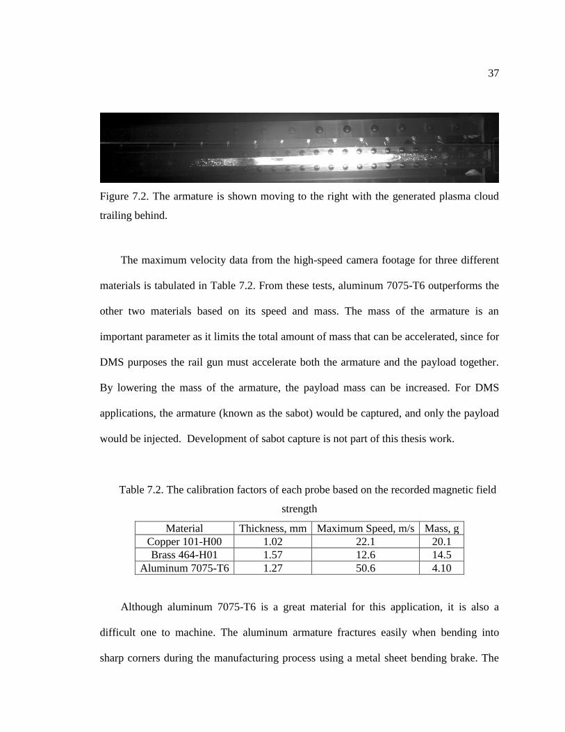
shown in Figure 7.2, there is an absence of plasma cloud ahead of the armature. This

indicates that the current from the power supply is largely driven through the armature,

rather than being wasted on accelerating the plasma cloud that may exist in front of the

armature. This means that there is good electrical contact between the armature and the

rails throughout the acceleration phase. This was one of the objectives of the armature

design and the experimental results show the armature is indeed maintaining good contact

with the rails.

37

Figure 7.2. The armature is shown moving to the right with the generated plasma cloud

trailing behind.

The maximum velocity data from the high-speed camera footage for three different

materials is tabulated in Table 7.2. From these tests, aluminum 7075-T6 outperforms the

other two materials based on its speed and mass. The mass of the armature is an

important parameter as it limits the total amount of mass that can be accelerated, since for

DMS purposes the rail gun must accelerate both the armature and the payload together.

By lowering the mass of the armature, the payload mass can be increased. For DMS

applications, the armature (known as the sabot) would be captured, and only the payload

would be injected. Development of sabot capture is not part of this thesis work.

Table 7.2. The calibration factors of each probe based on the recorded magnetic field

strength

Material Thickness, mm Maximum Speed, m/s Mass, g

Copper 101-H00 1.02 22.1 20.1

Brass 464-H01 1.57 12.6 14.5

Aluminum 7075-T6 1.27 50.6 4.10

Although aluminum 7075-T6 is a great material for this application, it is also a

difficult one to machine. The aluminum armature fractures easily when bending into

sharp corners during the manufacturing process using a metal sheet bending brake. The

38

armatures for the latter tests are manufactured using a waterjet fabrication process.

Waterjet allows for precise manufacturing and reduces the amount of strain added to the

material during manufacturing. It also provides consistency in the armature’s geometry

over multiple fabrications.

After a series of test shots, the erosion on the rails became significant creating

uneven surfaces, leading to poor acceleration of the armature. One of the main problems

was the change in bore cross-section, as the armature material is transferred onto the

surface of the rails after each shot. To reduce this erosion effect, for the next series of test

fires, the surfaces of the electrodes and the tips of the armatures were plasma sprayed

with coatings of tungsten using a plasma spray process.

7.2 EXTERNAL FIELD AUGMENTATION

As previously described in Chapter 4, the force acting on the armature can be increased

with the introduction of an external magnetic field. This external magnetic field needs to

be aligned correctly with the direction of the field that the rail gun generates. In this

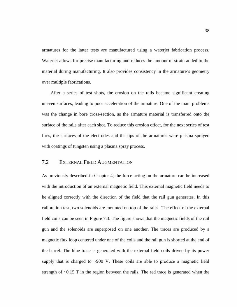
calibration test, two solenoids are mounted on top of the rails. The effect of the external

field coils can be seen in Figure 7.3. The figure shows that the magnetic fields of the rail

gun and the solenoids are superposed on one another. The traces are produced by a

magnetic flux loop centered under one of the coils and the rail gun is shorted at the end of

the barrel. The blue trace is generated with the external field coils driven by its power

supply that is charged to ~900 V. These coils are able to produce a magnetic field

strength of ~0.15 T in the region between the rails. The red trace is generated when the

39

rail gun is operated with the capacitors charged up to ~900 V. The rail guns produce a

magnetic field strength of ~0.48 T. When both systems (the rail gun and the augmented

coils) are operated, with a trigger delay of 7.50 ms between the firing of the solenoid and

the firing of the rail gun, the total magnetic field is about ~0.62 T.

Figure 7.3. The figure shows the magnetic field strength added to the rail gun system by

augmenting solenoids.

The effect of the external field coil is to increase the effective magnetic field

experienced by the armature. This allows for a stronger Lorentz force, hence a better

acceleration without the need to increase the current through the rail gun system. This is

particularly important during the early stage of acceleration when the current is low. A

40

reduction of the driving current means that the heating in the armature would also be

reduced. Thus, the external field is a highly-desired feature as it would prolong the life-

time of components and increase the attainable velocity.

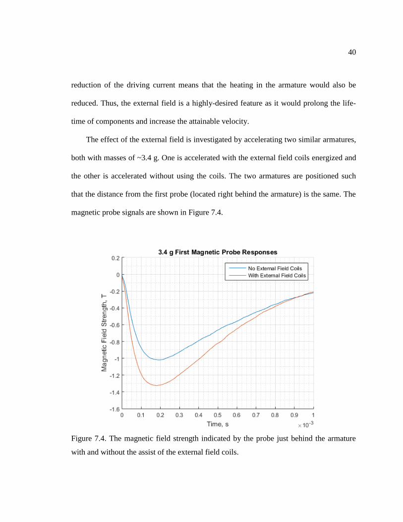
The effect of the external field is investigated by accelerating two similar armatures,

both with masses of ~3.4 g. One is accelerated with the external field coils energized and

the other is accelerated without using the coils. The two armatures are positioned such

that the distance from the first probe (located right behind the armature) is the same. The

magnetic probe signals are shown in Figure 7.4.

Figure 7.4. The magnetic field strength indicated by the probe just behind the armature

with and without the assist of the external field coils.

41

The coils are powered by a separate power supply that is charged to ~1.35 kV. The

differences in the first probe show the additional magnetic field strength added to the

system. The difference between the peaks is ~ 0.3 T, a ~30% increase over the system

without external field coils. As shown below, the additional magnetic field effect causes a

dramatic increase in the armature maximum velocity, although the field enhancement is

only 30%. What this means is that the initial force which now increases in proportion to

the current instead of as the square of the current, I2, is quite important when the initial

current is small, during the current rise phase. For systems with a short current pulse

(such as for DMS applications) and with small armature mass, the field enhancement may

be essential for reducing the energy deposited in the small armature, and needs to be

investigated as part of future development work.

42

Figure 7.5. The numerical simulations are presented in green and pink. The pink trace is

generated with 0.30 T of external magnetic field and the green trace is generated without

any external field. The figure shows current through the system, in kA, the traveled

distance, in cm, the instantaneous velocity, in km/s, and capacitor voltage, in kV. The

results, captured by the magnetic probes, from actual test fires are shown as scattered

marks over the simulations.

In Figure 7.5, the position of the armature is well predicted compared to the

numerical simulations done with the governing equations with the added external

magnetic field. A slight variation in the distance plot is expected, as there exist a

changing external magnetic field in the external coil that is not taken into consideration in

43

the numerical simulations. The experimental velocity data is generated based on

measurements from two adjacent probes, which have a finite and large separation

distance. Even with the limited data entries, the recorded data match well with the

numerical predictions. The armature without the external field achieved a maximum

velocity of ~80 m/s while the one accelerated with the augmented field coils achieved a

maximum velocity of ~110 m/s. The rail gun power supply held a charge of ~2 kV in

both cases. The power supply for the external field coils was charged to ~1.35 kV for the

case where augmented coils are operated. The improvement in speed for the augmented

case is clearly desirable, since the injection speed determines the distance the radiative

materials can penetrate in the plasma. It is useful to note that in a tokamak setting, the

external magnetic field is free and available if the injector can be located close to the

vessel, which also helps to reduce the system response time.

7.3 VARYING ARMATURE THICKNESS

Although aluminum 7075-T6 is the most appropriate of the available materials for this

experiment through earlier testing, the thickness of the armature is still a parameter to be

considered, as for the final application an armature with the least mass consistent with

adequate strength at the operating conditions is desired. A batch of water-jetted armatures

with thicknesses varying between ~0.838 to 1.27 mm was manufactured, and the

corresponding masses and test numbers tabulated in Table 7.3.

44

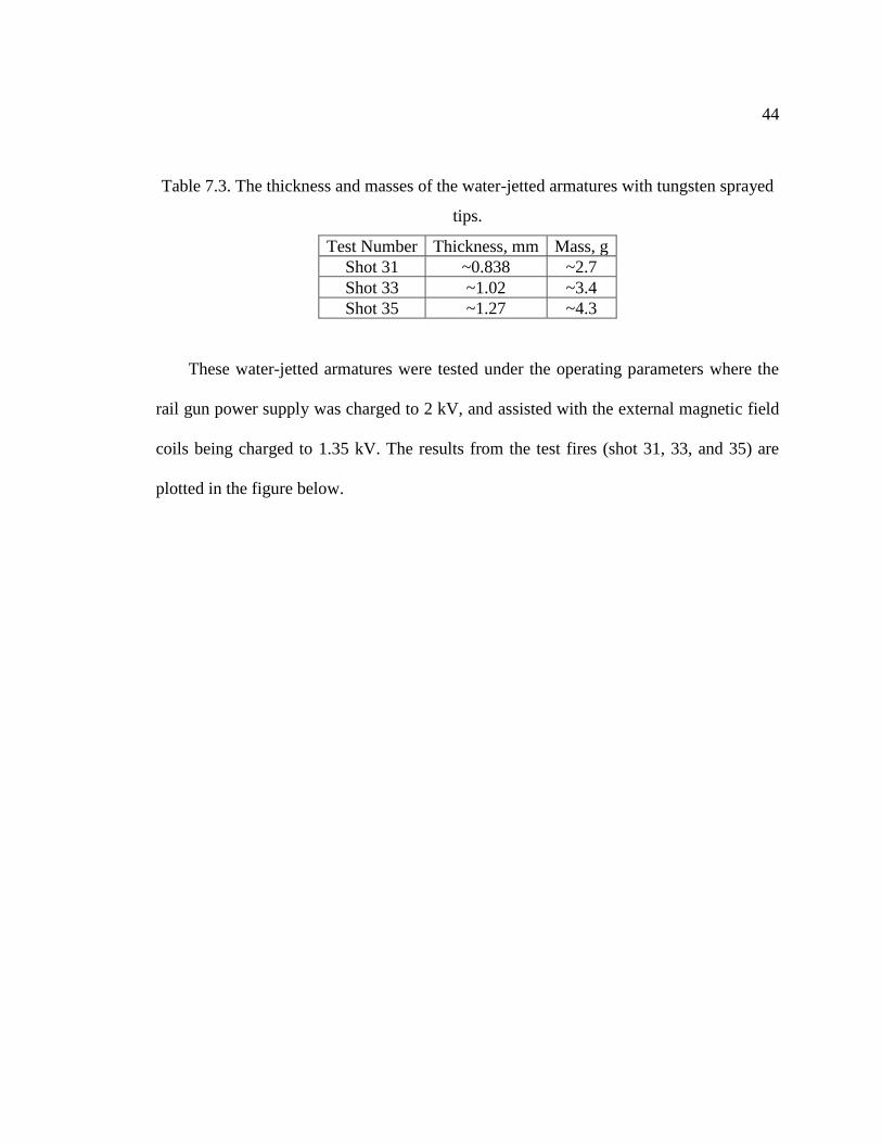
Table 7.3. The thickness and masses of the water-jetted armatures with tungsten sprayed

tips.

Test Number Thickness, mm Mass, g

Shot 31 ~0.838 ~2.7

Shot 33 ~1.02 ~3.4

Shot 35 ~1.27 ~4.3

These water-jetted armatures were tested under the operating parameters where the

rail gun power supply was charged to 2 kV, and assisted with the external magnetic field

coils being charged to 1.35 kV. The results from the test fires (shot 31, 33, and 35) are

plotted in the figure below.

45

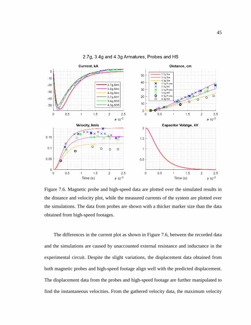
Figure 7.6. Magnetic probe and high-speed data are plotted over the simulated results in

the distance and velocity plot, while the measured currents of the system are plotted over

the simulations. The data from probes are shown with a thicker marker size than the data

obtained from high-speed footages.

The differences in the current plot as shown in Figure 7.6, between the recorded data

and the simulations are caused by unaccounted external resistance and inductance in the

experimental circuit. Despite the slight variations, the displacement data obtained from

both magnetic probes and high-speed footage align well with the predicted displacement.

The displacement data from the probes and high-speed footage are further manipulated to

find the instantaneous velocities. From the gathered velocity data, the maximum velocity

46

in all three cases occurred within the 1.5 ms after the system was energized, which

indicates that the response time of the system is indeed very rapid as desired for DMS

application. The second objective of obtaining the projected velocity is also demonstrated

in this experiment. This means that the test bench setup has a response time on the order

of ~2 ms after the rail gun power supply is triggered. The maximum achieved velocity for

~2.7 g, ~3.4 g and ~4.3 g is ~173 m/s, ~150 m/s and ~105 m/s, respectively. These tests

show that the increase in velocity of the armature occurs with the reduction in armature

mass, consistent with the projections. The data clearly shows that the response time of

this rail gun configuration is indeed rapid and can only be further improved with a further

increase in the ambient magnetic field strength.

7.4 SCALING UP FOR NSTX-U AND ITER

The numerical simulations up to this point have well predicted the performance of the

small rail gun system. To achieve the desired goal for ITER, the payload, with ~15 g

mass composed of radiative materials such as boron, boron nitride or beryllium, must be

accelerated to a velocity upwards of 1 km/s.

47

Figure 7.7. Shown are numerical simulations for accelerating the required payload with

0 T, 2 T, 4 T ambient fields, represented as ITER A, ITER B, ITER C, respectively.

From Figure 7.7, ITER A case shows the injector being powered by a 100 mF power

supply that is charged up to 4.5 kV. The simulation shows that the armature will achieve

its desired velocity of ~1 km/s at about 0.86 ms. This means the total injector length does

not need to be more than 50 cm long. The current plot shows a maximum current of

~340 kA. Now, if the system is exposed to a 2 T external magnetic field shown as

ITER B, the same capacitor bank only needs to be charged up to 3.2 kV to achieve a

similar velocity profile while reducing the maximum current to ~240 kA. If the system

48

has a surrounding magnetic field of 4 T, the power supply voltage requirement is now

reduced to just 2.2 kV. While maintaining a comparable velocity trace, the current of the

system is further reduced to ~170 kA. From these numerical simulations, the beneficial

effects of an external magnetic field are shown to be highly desirable. With a strong

external magnetic field, the power supply can be less complicated as the energy

requirement is reduced. Also, the current through the system is further reduced which

help to suppress electrode erosion and prolong electrode life.

If this system is mounted 5 m away from the plasma’s edge, with an injection

velocity of 1 km/s, the total response time is <10 ms. This is considerably faster than the

Massive Gas and the Cryogenic Pellet methods (which are on the order of~ 20 to 30 ms.)

Additionally, the EPI system can be mounted very close to the vessel of the reactor,

unlike its gas dependent counterparts, as it has no mechanical moving parts or plastics.

This would further reduce the response time to less than 3 ms, which is very rapid

compared to any other system that is considered for DMS applications.

49

Chapter 8. CONCLUSION

The EPI system, based on a simple linear rail gun concept, was built at the University of

Washington, to test its potential for DMS application for fusion reactor applications.

Consistent with calculations, the experimental study finds that it is capable of rapid

response on the order of ~2 ms after it is initiated. The system is capable of propelling a

mass of 3.4 g to the predicted attainable velocities (~150 m/s) on a fast time scale with

augmented electromagnets. The new armature design introduces spring-like properties to

allow better contact with the rails and seems to be effective in avoiding plasma expansion

in front of the armature. Unlike current DMS methods, the projected EPI system has

higher projected velocity injection, which should allow for deeper penetration of radiative

payloads into ITER’s plasma. Also, due to the lack of mechanical components, lack of

plastic materials in its design, and small dimensions (~50 cm), the system can be

deployed in close proximity to a fusion tokamak reactor vessel. With an ambient

magnetic field of 3-4 T near the vessel, the performance of the EPI system would be

dramatically enhanced. The strong magnetic field augmentation would also prolong the

lifetime of the rail gun due to reduced electrode erosion. The supporting power supply

needs would also be simplified due to reduced driving current requirements.

As a next step of this study, a system with refractory rail materials should be built,

to allow for more extensive testing without the need for frequent resurfacing. Also, the

50

next system should include a vacuumed barrel design to better simulate the environment

of a tokamak setting. Finally, the benefits of external magnetic field augmentation should

be investigated in more detail. With the extremely encouraging results from this study,

the application of a rail gun based DMS appears to a viable concept that clearly warrants

further study.

51

BIBLIOGRAPHY

[1] R. Raman, T. R. Jarboe, B. A. Nelson, S. P. Gerhardt, W.-S. Lay and G. J. Plunkett,

"Design and Operation of a Fast Electromagnetic Inductive Massive Gas Injection

Valve for NSTX-U," Review of Scientific Instruments, vol. 85, pp. 11E801-1-

11E801-4, 2014.

[2] L. R. Baylor, S. Combs, C. R. Foust, T. C. Jernigan, S. J. Meitner, P. B. Parks, J. B.

Caughman, S. Maruyama, A. L. Qualls, D. A. Rasmussen and C. E. Thomas Jr.,

"Pellet Fueling, ELM pacing, and Disruption Mitigation Technology Development

for ITER," Nuclear Fusion, vol. 49, no. 8, pp. 1-8, 2009.

[3] S. K. Combs, L. Baylor, C. R. Foust, A. Frattolillo, M. S. Lyttle, S. J. Meitner and S.

Miglior, "Experimental Study of the Propellant Gas Load Required for Pellet

Injection with ITER-Relevant Operating Parameters," Fusion Science and

Technology, vol. 68, no. 2, pp. 219-325, 2015.

[4] R. Raman, T. R. Jarboe, J. E. Menard, S. P. Gerhardt, M. Ono, L. Baylor and W.-S.

Lay, "Fast Time Response Electromagnetic Disruption Mitigation Concept," Fusino

Science and Technology, vol. 68, pp. 797-805, November 2015.

[5] I. R. McNab, "Launch to Space With an Electromagnetic Railgun," IEEE

Transactions on Magnetics, vol. 39, no. 1, pp. 295-304, January 2003.

[6] E. Y. Choueiri, "New dawn of electric rocket," Scientific American, vol. 300, no. 2,

pp. 58-65, Feburary 2009.

[7] R. Burton and P. Turchi, "Pulsed Plasma Thruster," Journal of Propulson and

Power, vol. 14, no. 5, pp. 716-735, September 1998.

[8] S. Snow, "U.S. May Field Railgun on Zumwalt Destroyer," 01 March 2016.

[Online]. Available: http://thediplomat.com/2016/03/u-s-may-field-railgun-on-

zumwalt-destroyer/. [Accessed 26 April 2017].

[9] J. Mcfarland and I. Mcnab, "A Long-Range Naval Railgun," IEEE Transactions on

Magnetics, vol. 39, no. 1, pp. 289-294, January 2003.

[10] E. M. Hollmann, T. C. Jernigan, E. J. Strait, M. Van Zeeland, J. C. Wesley, J. C.

West, W. Wu and J. Yu, "Measurements of injected impurity assimilation during

massive gas injection experiments in DIII-D," Nuclear Fusion, vol. 48, no. 11, pp.

115007-1-115007-12, 2008.

52

[11] M. Lehnen, A. Alonso, G. Arnoux, N. Baumgarten, S. Bozhenkov, S. Brezinsek, M.

Brix, T. Eich, S. Gerasimov, A. Huber, S. Jachmich, U. Kruezi, P. Morgan, V.

Plyusnin, C. Reux, V. Riccardo, G. Sergienko and M. Stamp, "Disruption Mitigation

by Massive Gas Injection in JET," Neclear Fusion, vol. 51, no. 12, pp. 123010-1-

123010-12, 2001.

[12] R. Raman, G. Plunkett and W.-S. Lay, "Massive Gas Injection Valve Development

for NSTX-U," IEEE Transactions on Plasma Science, vol. 44, no. 9, pp. 1547-1552,

2016.

[13] E. M. Hollmann, P. B. Aleynikov, T. Fülöp, D. A. Humphreys, V. A. Izzo, M.

Lehnen, V. E. Lukash, G. Papp, G. Pautasso, F. Saint-Laurent and J. A. Snipes,

"Status of research toward the ITER disruption mitigation system," Physics of

Plasmas, vol. 22, pp. 021802-1-021802-16, February 2015.

[14] L. R. Baylor, C. C. Barbier, J. R. Carmichael, S. K. Combs, M. N. Ericson, N. D.

Bull Ezell, P. W. Fisher, M. S. Lyttle, S. J. Meitner, D. A. Rasmussen, S. F. Smith, J.

B. Wilgen, S. Maruyama and G. Kiss, "Disruption Mitigation System Developments

and Design for ITER," Fusion Science and Technology, vol. 68, pp. 211-215,

September 2015.

[15] V. Leonov, V. Zhogolev, S. Konovalov and M. Lehnen, "Simulation of the Pre-

Thermal Quench Stage of Disruptions During Massive Gas Injection and Projections

for ITER," in 2014 25th IAEA Fusion Energy Conference, St Pertersburg, 2014.

[16] V. Izzo, "A numerical investigation of the effects of impurity penetration depth on

disruption mitigation by massive high-pressure gas jet," Nuclear Fusion, vol. 46, no.

5, pp. 541-547, 2006.

[17] E. M. Hollmann, N. Commaux, N. W. Eidietis, D. A. Humphreys, T. J. Jernigan, C.

J. Lasnier, R. A. Moyer, R. A. Pitts, M. Sugihara, E. J. Strait, J. Watkins and J. C.

Wesley, "Characterization of heat loads from mitigated and unmitigated vertical

displacement events in DIII-D," Physics of Plasmas, vol. 20, no. 6, pp. 062501-1-

062501-9, June 2013.

[18] N. J. Commaux, L. R. Baylor, T. C. Jernigan, E. M. Hollmann, P. B. Parks, D. A.

Humphrey, J. C. Wesley and J. Yu, "Demonstration of rapid shutdown using large

shattered deuterium pellet injection in DIII-D," Nuclear Fusion, vol. 50, no. 11, p.

112001, 2010.

[19] N. Commaux, D. Shiraki, L. Baylor, E. Hollmann, N. Eidietis, C. Lasnier, R. Moyer,

T. Jernigan, S. Meitner, S. Combs and C. Foust, "First demonstration of rapid

shutdown using neon shattered pellet injection for thermal quench mitigation on diii-

d," Nuclear Fusion, vol. 56, no. 4, pp. 046007-1-046007-7, 2016.

[20] J. Hammer, C. Hartman, J. Eddleman and H. McLean, "Experimental Demonstration

of Acceleration and Focusing of Magnetically Confined Plasma Rings," Physics

Review Letters, vol. 61, no. 25, pp. 2843-2846, 1988.

53

[21] M. S. Bayati and A. Keshtkar, "Study of the Current Distribution, Magnetic Field,

and Inductance Gradient of Rectangular and Circular Railguns," IEEE Transactions

on Plasma Science, vol. 41, no. 5, pp. 1376-1381, May 2013.

[22] A. Keshtkar, A. Kalantarnia and M. Kiani, "Improvement of Inductance Gradient in

Railgun Using Ferromagnetic Materials," in 2008 14th Symposium on

Electromagnetic Launch Technology, Victoria, 2008.

[23] S. Katsuki, H. Akiyama, N. Eguchi, T. Sueda, M. Soejima, S. Maeda and K. N. Sato,

"Augmented Railgun Using a Permanent Magnet," Review of Scientific Instruments,

vol. 66, no. 8, pp. 4227-4232, August 1995.

[24] L. Chen, J. He, Z. Xiao, S. Xia, D. Feng and L. Tang, "Experimental Study of

Armature Melt Wear in Solid Armature Railgun," IEEE Transactions on Plasma

Science, vol. 43, no. 5, pp. 1142-1146, 16 April 2015.

[25] S. Starr, R. Youngquist and R. Cox, "A Low Voltage "Railgun"," American Journal

of Physics, vol. 81, no. 1, pp. 38-43, January 2013.

[26] A. Keshtkar, S. Bayati and A. Keshtkar, "Derivation of a Formula for Inductance

Gradient Using Intelligent Estimation Method," IEEE Transactions on Magnetics,

vol. 45, no. 1, pp. 305-308, January 2009.

[27] J. Dormand and P. Prince, "A family of embedded Runge-Kutta formulae," Journal

of Computational and Applied Mathematics, vol. 6, no. 1, pp. 19-26, 1980.