Effect of Tip Geometry on a Hovering Rotor in Ground ... · Eﬀect of Tip Geometry on a Hovering...

Effect of Tip Geometry on a Hovering Rotor in

Ground Effect:

A Computational Study

Tarandeep S. Kalra∗,

Vinod K. Lakshminarayan†,

James D. Baeder ‡

A compressible Reynolds Averaged Navier Stokes (RANS) is used to simulate a hov-ering rotor with four different tip shapes (rectangular, swept, BERP-like and slotted) tounderstand the effect of rotor wake in-ground effect(IGE). The simulations are built uponan original framework developed by the current authors. The tip vortices are better re-solved by modifying grids in order to follow the path of the rotor wake and using oversetmeshes to better preserve the vortices. Overall the fully turbulent RANS computationspredict a highly diffused vortex core compared to experiments for the rectangular, sweptand BERP-like tip. The eddy viscosity levels are quite high and it is believed that thecurrent formulation of turbulence modeling is leading to excessive diffusion of vorticity. Tocircumvent this problem, simulations are performed with the laminar flow assumption onthe wake capturing meshes. The tip vortices are captured well by using this assumptionand the tip vortex characteristics agree well with the experiments. Between the differenttip shapes, the rectangular and swept tip show similar vortex strengths. The BERP-liketip has a slightly diffused vortex core than the former two tip shapes. The slotted tip showsa highly diffused vortex core compared to the other three tips.

Nomenclature

A Area of the rotor blades (πR2)AR Aspect Ratio, AR = R/cc Rotor blade chordCP Rotor power coefficient in-ground effect = Power/(ρπR2V 3

tip)CT Rotor thrust coefficient in-ground effect = Thrust/(ρπR2V 2

tip)Mtip Tip Mach numberr Radial distancerc Vortex core radiusR Radius of the rotorRe Reynolds numberVtip Tip speedVθ Swirl velocityz Rotor height above groundΓ Circulationψ Wake age (degrees)θo Collective pitch (degrees)

∗ Graduate Research Assistant, [email protected]† Postdoctoral Fellow, [email protected]‡ Associate Professor, [email protected]

1 of 18

American Institute of Aeronautics and Astronautics

Dow

nloa

ded

by S

TA

NFO

RD

UN

IVE

RSI

TY

on

July

19,

201

3 | h

ttp://

arc.

aiaa

.org

| D

OI:

10.

2514

/6.2

013-

2542

31st AIAA Applied Aerodynamics Conference

June 24-27, 2013, San Diego, CA

AIAA 2013-2542

Copyright © 2013 by the American Institute of Aeronautics and Astronautics, Inc. All rights reserved.

I. Introduction

The brownout phenomenon consists of the creation of a dense dust cloud that engulfs the rotorcraft duringin-ground effect operation. Apart from the obvious problem of rendering the pilot visually disoriented, theseclouds can also be responsible for blade erosion and mechanical wear. Current day workarounds to thebrownout problem include the use of sensors and avionic displays for improving the situational awareness orthe employment of piloting strategies to avoid the brownout cloud. Although these solutions can contributein limiting the number of brownout related mishaps, these strategies only provide a temporary solution anda more permanent solution is desired for this problem. Since the interaction of the rotor wake with thedust particles on the ground is the driving force of the brownout phenomenon, it is believed that a goodunderstanding of the underlying flow physics can provide insight to develop effective means of preventingand/or mitigating the adverse effects of rotorcraft brownout.

Over the last few years, significant strides have been made in the experimental analysis of the brownoutproblem in controlled environments. Detailed particle image velocimetry (PIV) measurements of the flowfieldperformed by Lee et al.1 at micro scale and Milluzzo et al.2 at subscale showed a whole host of aerodynamicphenomena such as diffusion, vortex stretching and turbulence generation occurring close to the ground.PIV measurements enabled the experimentalists to measure the velocity profiles close to the ground for aquantitative estimate of the flowfield. Recent experiments have been performed by Hance et al.3 to includethe effect of fuselage on the wake of a two-bladed subscale rotor. Additional experiments conducted byJohnson et al.4 and Sydney et al.5 showed the phenomenon of entrainment and uplift of sediment particlesin the presence of the rotor wake of a hovering micro scale rotor. Other experimental studies include thePIV measurements and brownout simulations performed by Nathan and Green.6 These experiments wereconducted in a wind tunnel to simulate low speed forward flight on a micro scale rotor.

These aforementioned experiments provide a detailed understanding of the fluid dynamics for micro andsubscale rotor in-ground effect. However, the wide range of parameters affecting the brownout problem arestill difficult to model in experiments. The main experimental difficulty comes in simulating the brownoutconditions in full-scale rotors. Computational studies can be used to overcome these challenges by simulatinga wide range of brownout conditions with relative ease. However, computational studies have their own shareof challenges such as:

• The tip vortex emanating from the blade needs to be preserved for a significantly long time to capturetheir interaction with the ground, and therefore, can be computationally expensive, especially whenthe ground distances are large.

• It is necessary to resolve the boundary layer and the turbulence at the ground, which can be extremelychallenging especially using non-CFD computational methods.

• Modeling the fluid-particle interaction for these complicated flow-field is extremely challenging. Devel-opment of a particle model is still an active field of research.

These challenges are further aggravated in terms of computational expense when the scale of the problemis increased. To simplify the computations, most recent studies simplify the multi-phase brownout problem byignoring the effects of the airborne sediment particles on the flowfield and simulate only the effect of flowfieldon the particles. This is a reasonable approximation for the brownout problem, except possibly very close tothe ground where the particle density cloud may be large enough to affect the momentum of the fluid. Thisdecoupled approach allows one to concentrate on the problem of tracking the evolution of the rotor tip vorticesand its interaction with the ground boundary layer. Over the last few years, researchers modeling brownouthave employed aerodynamic models of various levels of sophistication. Most approaches track the tip vortexin the particle-fixed Lagrangian frame of reference.7–9 Even though these free-vortex type methods can trackthe vortex for a long distance, these methods involve a certain degree of empiricism in determining the vortexcore radius and roll-up. Additionally, these methods rely on approximate sublayer models to predict theground boundary layer and thus may be best suited to provide qualitative prediction of the ground boundarylayer. Methods using the vorticity transport model (VTM)10–12 or vorticity confinement13,14 provide acapability for a more fundamental representation of the formation and evolution of the tip vortex. However,VTM applications to brownout have been run as an inviscid model and thus still require an approximationto the sublayer to capture the ground boundary layer. On the other hand, vorticity confinement applicationsto brownout have used very coarse meshes near the ground that may not be sufficient to capture the details

2 of 18


Dow

nloa

ded

by S

TA

NFO

RD

UN

IVE

RSI

TY

on

July

19,

201

3 | h

ttp://

arc.

aiaa

.org

| D

OI:

10.

2514

/6.2

013-

2542


of the wall jet and interaction with the vortical wake. Furthermore, in these studies the blades were treatedusing lifting-line aerodynamics with their accompanying assumptions. In another work, Thomas et al.15

presented a hybrid methodology combining the capabilities of a high-fidelity RANS solver with a free-wakemethod to simulate the single-phase and two-phase flowfield environment beneath a hovering rotor. Thismethod requires lesser computational expense compared to a full RANS single-phase simulation but stillrelies on empirical correlations in the free-wake domain of the flowfield. Thus, all the above mentionedapproaches in their current forms still retain a fair amount of empiricism.

A RANS-based CFD solver with sufficient mesh resolution can resolve the detailed velocity profiles nearthe ground without using empirical vortex core factors or a sublayer model. The primary disadvantage of thismethodology is the computational expense required to capture the evolution of the wake structure. However,with parallelization and the use of intelligent clustering of mesh points in regions of interest, one can usethese high fidelity methods to simulate the brownout problem. Earlier work by current authors 16 and 17

showed the capability of this methodology to provide accurate performance and flowfield characteristics ofthe micro scale rotor tested by Lee et al.1 The current work extends this methodology to simulate the one-bladed subscale rotor experiments of Milluzzo et al.2 The simulations investigate the effect of four differentblade tip shapes on the tip vortex formation, evolution and its interaction with the ground.

II. Experimental Setup for Validation

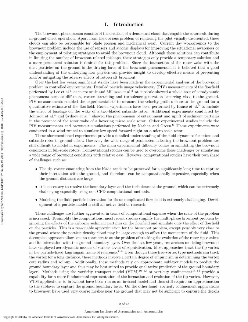
The experimental setup of Milluzzo et al.2 shown in fig. 1 is used to validate the flowfield of a hoveringone-bladed rotor operating in-ground effect. The rotor consisted of an untwisted rectangular blade withNACA 2415 airfoil. The rotor blades had an aspect ratio of 9.132 and were set to a collective pitch of 4.5◦.The rotor operated at a tip Mach number of 0.24 and a chord Reynolds number of 250, 000. The experimentswere performed on four different blades obtained by varying the blade tip shapes. The rotor blades operatedat a rotor height of 1R above ground.

Figure 1. Experimental setup of Mullizzo et.al.

III. Methodology

III.A. Flow Solver

In the present work, a RANS based solver OVERTURNS18 is used to perform the computations in a time-accurate manner in an inertial frame of reference. The code solves the compressible RANS equations using apreconditioned dual-time scheme. The second order backwards differening scheme is used for time marchingand the linear system is solved using Lower Upper Symmetric Gauss Seidel (LUSGS) framework. Low Mach

3 of 18


Dow

nloa

ded

by S

TA

NFO

RD

UN

IVE

RSI

TY

on

July

19,

201

3 | h

ttp://

arc.

aiaa

.org

| D

OI:

10.

2514

/6.2

013-

2542


preconditioning22 is used to improve the convergence and accuracy of the flow solver. A third-order MUSCLscheme23 utilizing Koren’s limiter24 is used for spatial reconstruction on the blade and the main backgroundmesh and a fifth-order mapped WENO scheme25 scheme is used vortex tracking grids and funnel shapedmesh. More details about the meshes are provided in the following section. The Roe flux difference scheme26

is used for calculating inviscid fluxes and a second-order central scheme is used to discretize the viscous terms.The Spalart-Allmaras27 turbulence model is employed for the RANS closure. This one-equation model hasthe advantages of ease of implementation, computational efficiency and numerical stability. The productionterm in this eddy-viscosity model is modified to account for the reduction in turbulence levels at the vortexcore due to rotational effects.28 The implicit hole-cutting technique, developed by Lee29 and improved byLakshminarayan,18 is used to determine the connectivity information between the various overset meshes.

III.B. Mesh System

III.B.1. Blade meshes for four different tip shapes

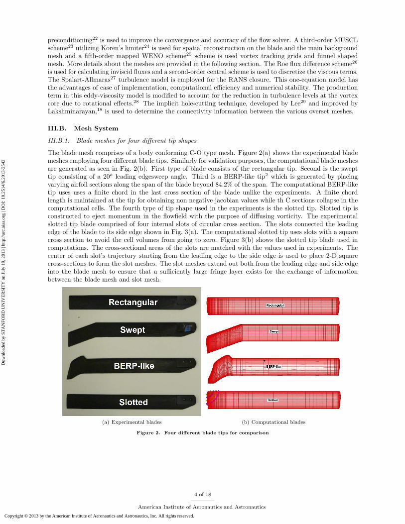
The blade mesh comprises of a body conforming C-O type mesh. Figure 2(a) shows the experimental blademeshes employing four different blade tips. Similarly for validation purposes, the computational blade meshesare generated as seen in Fig. 2(b). First type of blade consists of the rectangular tip. Second is the swepttip consisting of a 20o leading edgesweep angle. Third is a BERP-like tip2 which is generated by placingvarying airfoil sections along the span of the blade beyond 84.2% of the span. The computational BERP-liketip uses uses a finite chord in the last cross section of the blade unlike the experiments. A finite chordlength is maintained at the tip for obtaining non negative jacobian values while th C sections collapse in thecomputational cells. The fourth type of tip shape used in the experiments is the slotted tip. Slotted tip isconstructed to eject momentum in the flowfield with the purpose of diffusing vorticity. The experimentalslotted tip blade comprised of four internal slots of circular cross section. The slots connected the leadingedge of the blade to its side edge shown in Fig. 3(a). The computational slotted tip uses slots with a squarecross section to avoid the cell volumes from going to zero. Figure 3(b) shows the slotted tip blade used incomputations. The cross-sectional areas of the slots are matched with the values used in experiments. Thecenter of each slot’s trajectory starting from the leading edge to the side edge is used to place 2-D squarecross-sections to form the slot meshes. The slot meshes extend out both from the leading edge and side edgeinto the blade mesh to ensure that a sufficiently large fringe layer exists for the exchange of informationbetween the blade mesh and slot mesh.

(a) Experimental blades (b) Computational blades

Figure 2. Four different blade tips for comparison

4 of 18


Dow

nloa

ded

by S

TA

NFO

RD

UN

IVE

RSI

TY

on

July

19,

201

3 | h

ttp://

arc.

aiaa

.org

| D

OI:

10.

2514

/6.2

013-

2542


(a) Experimental slot mesh (b) Computational slot mesh

Figure 3. Experimental and computational slot tips

III.B.2. Overset meshes for wake capturing

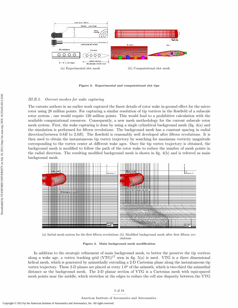
The curents authors in an earlier work captured the finest details of rotor wake in-ground effect for the microrotor using 28 million points. For capturing a similar resolution of tip vortices in the flowfield of a subscalerotor system , one would require 128 million points. This would lead to a prohibitive calculation with theavailable computational resources. Consequently, a new mesh methodology for the current subscale rotormesh system. First, the wake capturing is done by using a single cylindrical background mesh (fig. 4(a) andthe simulation is performed for fifteen revolutions. The background mesh has a constant spacing in radialdirection(between 0.8R to 2.0R). The flowfield is reasonably well developed after fifteen revolutions. It isthen used to obtain the instantaneous tip vortex trajectory by searching for maximum vorticity magnitudecorresponding to the vortex center at different wake ages. Once the tip vortex trajectory is obtained, thebackground mesh is modified to follow the path of the rotor wake to reduce the number of mesh points inthe radial direction. The resulting modified background mesh is shown in fig. 4(b) and is referred as mainbackground mesh.

(a) Initial mesh system for the first fifteen revolutions (b) Modified background mesh after first fifteen rev-olutions

Figure 4. Main background mesh modification

In addition to the strategic refinement of main background mesh, to better the preserve the tip vorticesalong a wake age, a vortex tracking grid (VTG)17 seen in fig. 5(a) is used. VTG is a three dimensionalhelical mesh, which is generated by azimuthally extruding a 2-D Cartesian plane along the instantaneous tipvortex trajectory. These 2-D planes are placed at every 1.0o of the azimuth, which is two-third the azimuthaldistance as the background mesh. The 2-D planar section of VTG is a Cartesian mesh with equi-spacedmesh points near the middle, which stretches at the edges to reduce the cell size disparity between the VTG

5 of 18


Dow

nloa

ded

by S

TA

NFO

RD

UN

IVE

RSI

TY

on

July

19,

201

3 | h

ttp://

arc.

aiaa

.org

| D

OI:

10.

2514

/6.2

013-

2542


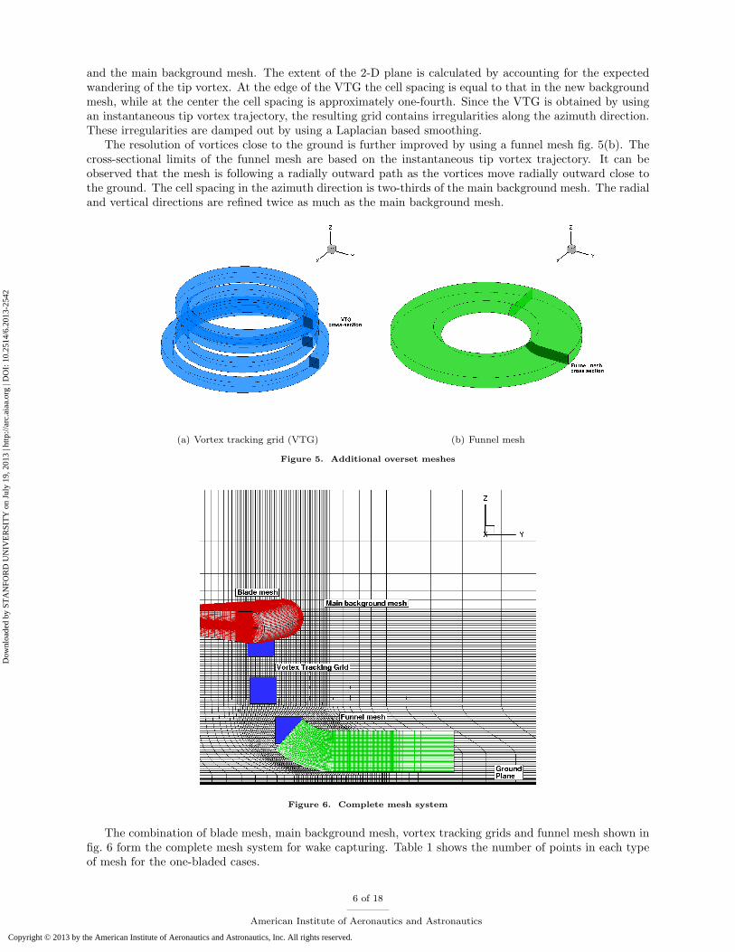
and the main background mesh. The extent of the 2-D plane is calculated by accounting for the expectedwandering of the tip vortex. At the edge of the VTG the cell spacing is equal to that in the new backgroundmesh, while at the center the cell spacing is approximately one-fourth. Since the VTG is obtained by usingan instantaneous tip vortex trajectory, the resulting grid contains irregularities along the azimuth direction.These irregularities are damped out by using a Laplacian based smoothing.

The resolution of vortices close to the ground is further improved by using a funnel mesh fig. 5(b). Thecross-sectional limits of the funnel mesh are based on the instantaneous tip vortex trajectory. It can beobserved that the mesh is following a radially outward path as the vortices move radially outward close tothe ground. The cell spacing in the azimuth direction is two-thirds of the main background mesh. The radialand vertical directions are refined twice as much as the main background mesh.

(a) Vortex tracking grid (VTG) (b) Funnel mesh

Figure 5. Additional overset meshes

Figure 6. Complete mesh system

The combination of blade mesh, main background mesh, vortex tracking grids and funnel mesh shown infig. 6 form the complete mesh system for wake capturing. Table 1 shows the number of points in each typeof mesh for the one-bladed cases.

6 of 18


Dow

nloa

ded

by S

TA

NFO

RD

UN

IVE

RSI

TY

on

July

19,

201

3 | h

ttp://

arc.

aiaa

.org

| D

OI:

10.

2514

/6.2

013-

2542


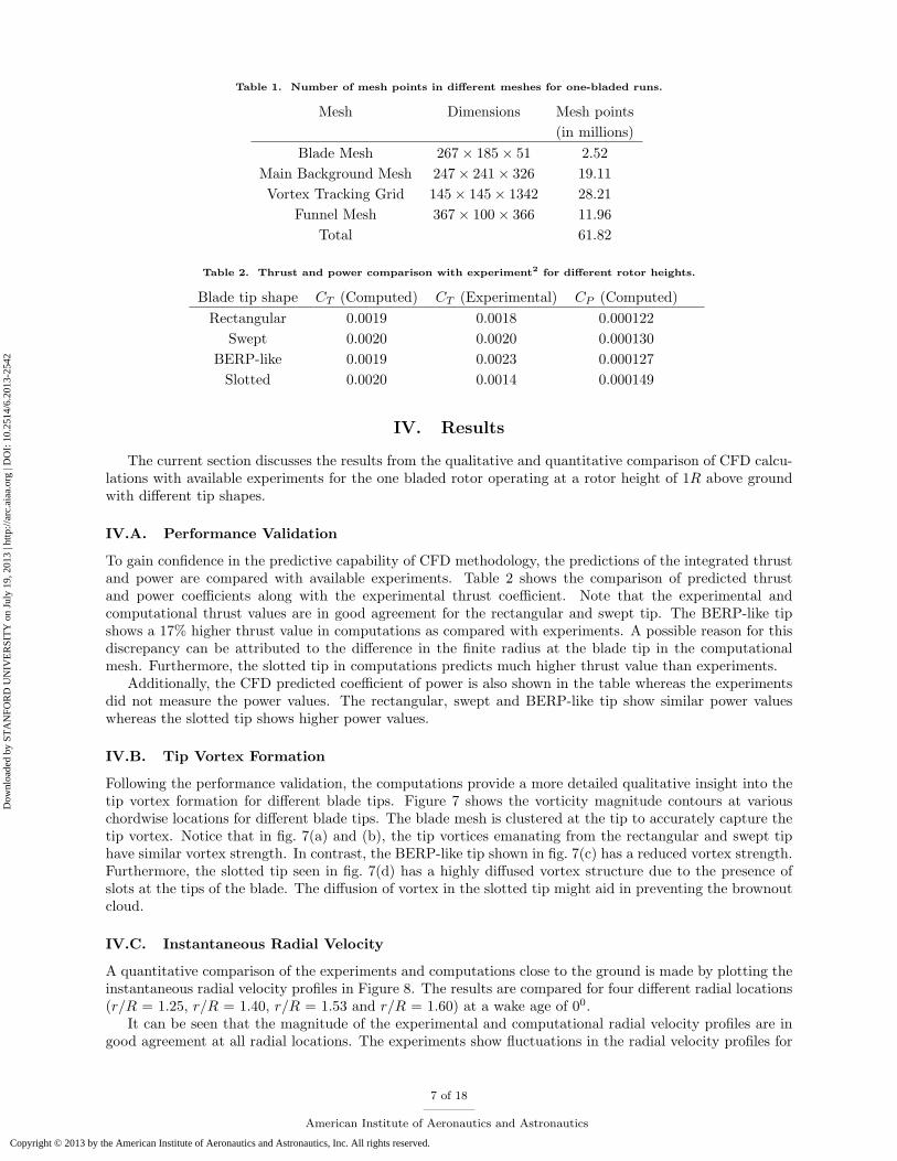
Table 1. Number of mesh points in different meshes for one-bladed runs.

Mesh Dimensions Mesh points

(in millions)

Blade Mesh 267 × 185 × 51 2.52

Main Background Mesh 247 × 241 × 326 19.11

Vortex Tracking Grid 145 × 145 × 1342 28.21

Funnel Mesh 367 × 100 × 366 11.96

Total 61.82

Table 2. Thrust and power comparison with experiment2 for different rotor heights.

Blade tip shape CT (Computed) CT (Experimental) CP (Computed)

Rectangular 0.0019 0.0018 0.000122

Swept 0.0020 0.0020 0.000130

BERP-like 0.0019 0.0023 0.000127

Slotted 0.0020 0.0014 0.000149

IV. Results

The current section discusses the results from the qualitative and quantitative comparison of CFD calcu-lations with available experiments for the one bladed rotor operating at a rotor height of 1R above groundwith different tip shapes.

IV.A. Performance Validation

To gain confidence in the predictive capability of CFD methodology, the predictions of the integrated thrustand power are compared with available experiments. Table 2 shows the comparison of predicted thrustand power coefficients along with the experimental thrust coefficient. Note that the experimental andcomputational thrust values are in good agreement for the rectangular and swept tip. The BERP-like tipshows a 17% higher thrust value in computations as compared with experiments. A possible reason for thisdiscrepancy can be attributed to the difference in the finite radius at the blade tip in the computationalmesh. Furthermore, the slotted tip in computations predicts much higher thrust value than experiments.

Additionally, the CFD predicted coefficient of power is also shown in the table whereas the experimentsdid not measure the power values. The rectangular, swept and BERP-like tip show similar power valueswhereas the slotted tip shows higher power values.

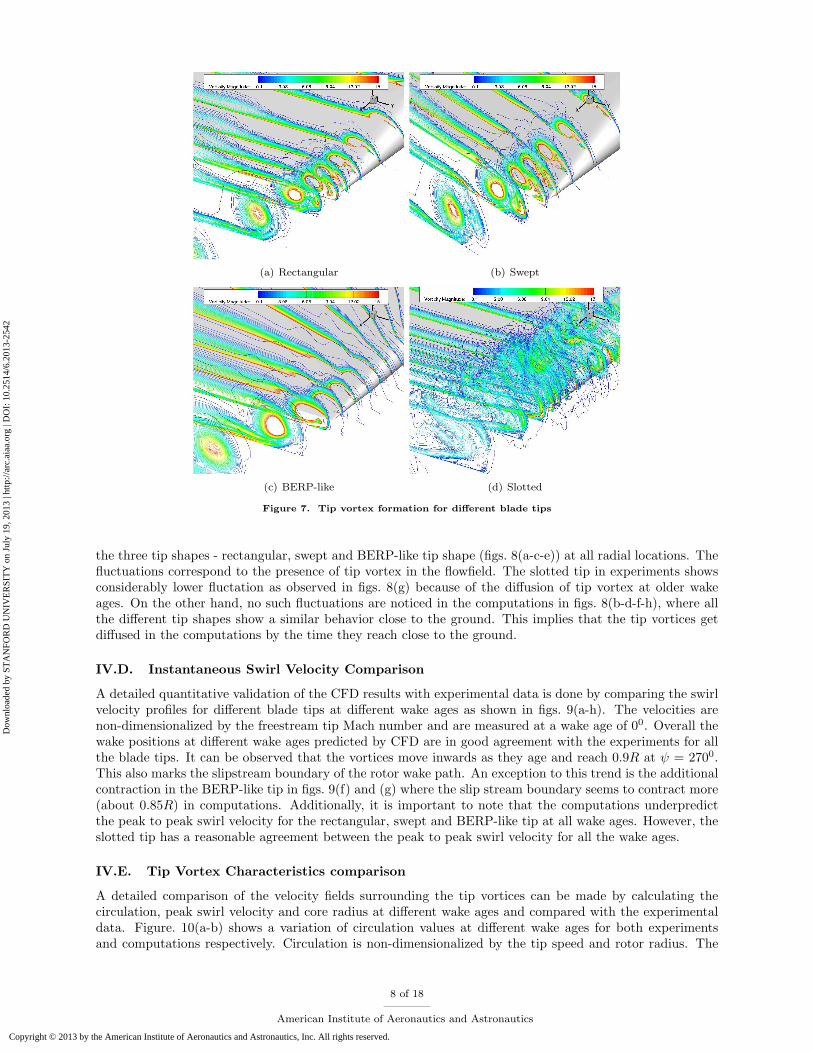
IV.B. Tip Vortex Formation

Following the performance validation, the computations provide a more detailed qualitative insight into thetip vortex formation for different blade tips. Figure 7 shows the vorticity magnitude contours at variouschordwise locations for different blade tips. The blade mesh is clustered at the tip to accurately capture thetip vortex. Notice that in fig. 7(a) and (b), the tip vortices emanating from the rectangular and swept tiphave similar vortex strength. In contrast, the BERP-like tip shown in fig. 7(c) has a reduced vortex strength.Furthermore, the slotted tip seen in fig. 7(d) has a highly diffused vortex structure due to the presence ofslots at the tips of the blade. The diffusion of vortex in the slotted tip might aid in preventing the brownoutcloud.

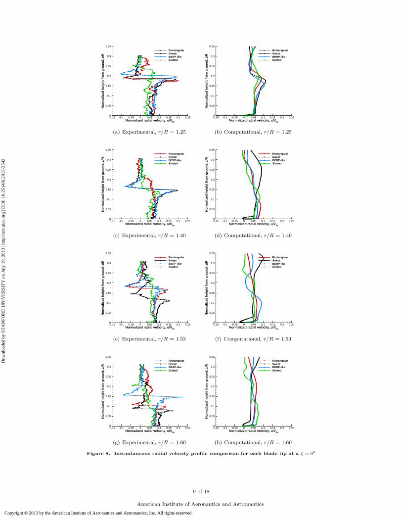
IV.C. Instantaneous Radial Velocity

A quantitative comparison of the experiments and computations close to the ground is made by plotting theinstantaneous radial velocity profiles in Figure 8. The results are compared for four different radial locations(r/R = 1.25, r/R = 1.40, r/R = 1.53 and r/R = 1.60) at a wake age of 00.

It can be seen that the magnitude of the experimental and computational radial velocity profiles are ingood agreement at all radial locations. The experiments show fluctuations in the radial velocity profiles for

7 of 18


Dow

nloa

ded

by S

TA

NFO

RD

UN

IVE

RSI

TY

on

July

19,

201

3 | h

ttp://

arc.

aiaa

.org

| D

OI:

10.

2514

/6.2

013-

2542


(a) Rectangular (b) Swept

(c) BERP-like (d) Slotted

Figure 7. Tip vortex formation for different blade tips

the three tip shapes - rectangular, swept and BERP-like tip shape (figs. 8(a-c-e)) at all radial locations. Thefluctuations correspond to the presence of tip vortex in the flowfield. The slotted tip in experiments showsconsiderably lower fluctation as observed in figs. 8(g) because of the diffusion of tip vortex at older wakeages. On the other hand, no such fluctuations are noticed in the computations in figs. 8(b-d-f-h), where allthe different tip shapes show a similar behavior close to the ground. This implies that the tip vortices getdiffused in the computations by the time they reach close to the ground.

IV.D. Instantaneous Swirl Velocity Comparison

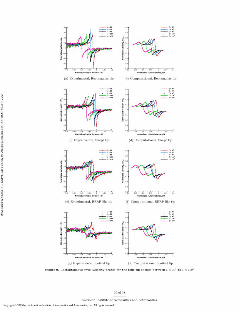
A detailed quantitative validation of the CFD results with experimental data is done by comparing the swirlvelocity profiles for different blade tips at different wake ages as shown in figs. 9(a-h). The velocities arenon-dimensionalized by the freestream tip Mach number and are measured at a wake age of 00. Overall thewake positions at different wake ages predicted by CFD are in good agreement with the experiments for allthe blade tips. It can be observed that the vortices move inwards as they age and reach 0.9R at ψ = 2700.This also marks the slipstream boundary of the rotor wake path. An exception to this trend is the additionalcontraction in the BERP-like tip in figs. 9(f) and (g) where the slip stream boundary seems to contract more(about 0.85R) in computations. Additionally, it is important to note that the computations underpredictthe peak to peak swirl velocity for the rectangular, swept and BERP-like tip at all wake ages. However, theslotted tip has a reasonable agreement between the peak to peak swirl velocity for all the wake ages.

IV.E. Tip Vortex Characteristics comparison

A detailed comparison of the velocity fields surrounding the tip vortices can be made by calculating thecirculation, peak swirl velocity and core radius at different wake ages and compared with the experimentaldata. Figure. 10(a-b) shows a variation of circulation values at different wake ages for both experimentsand computations respectively. Circulation is non-dimensionalized by the tip speed and rotor radius. The

8 of 18


Dow

nloa

ded

by S

TA

NFO

RD

UN

IVE

RSI

TY

on

July

19,

201

3 | h

ttp://

arc.

aiaa

.org

| D

OI:

10.

2514

/6.2

013-

2542


Normalized radial velocity, u/V tip

Nor

mal

ized

hei

ght f

rom

gro

und,

z/R

-0.15 -0.1 -0.05 0 0.05 0.1 0.15 0.2 0.250

0.05

0.1

0.15

0.2

0.25

0.3

0.35

RectangularSweptBERP-likeSlotted

(a) Experimental, r/R = 1.25


Nor

mal

ized

hei

ght f

rom

gro

und,

z/R

-0.15 -0.1 -0.05 0 0.05 0.1 0.15 0.2 0.250

0.05

0.1

0.15

0.2

0.25

0.3

0.35


(b) Computational, r/R = 1.25


Nor

mal

ized

hei

ght f

rom

gro

und,

z/R

-0.15 -0.1 -0.05 0 0.05 0.1 0.15 0.2 0.250

0.05

0.1

0.15

0.2

0.25

0.3

0.35


(c) Experimental, r/R = 1.40


Nor

mal

ized

hei

ght f

rom

gro

und,

z/R

-0.15 -0.1 -0.05 0 0.05 0.1 0.15 0.2 0.250

0.05

0.1

0.15

0.2

0.25

0.3

0.35


(d) Computational, r/R = 1.40


Nor

mal

ized

hei

ght f

rom

gro

und,

z/R

-0.15 -0.1 -0.05 0 0.05 0.1 0.15 0.2 0.250

0.05

0.1

0.15

0.2

0.25

0.3

0.35


(e) Experimental, r/R = 1.53


Nor

mal

ized

hei

ght f

rom

gro

und,

z/R

-0.15 -0.1 -0.05 0 0.05 0.1 0.15 0.2 0.250

0.05

0.1

0.15

0.2

0.25

0.3

0.35


(f) Computational, r/R = 1.53


Nor

mal

ized

hei

ght f

rom

gro

und,

z/R

-0.15 -0.1 -0.05 0 0.05 0.1 0.15 0.2 0.250

0.05

0.1

0.15

0.2

0.25

0.3

0.35


(g) Experimental, r/R = 1.60


Nor

mal

ized

hei

ght f

rom

gro

und,

z/R

-0.15 -0.1 -0.05 0 0.05 0.1 0.15 0.2 0.250

0.05

0.1

0.15

0.2

0.25

0.3

0.35


(h) Computational, r/R = 1.60

Figure 8. Instantaneous radial velocity profile comparison for each blade tip at a ζ = 0◦

9 of 18


Dow

nloa

ded

by S

TA

NFO

RD

UN

IVE

RSI

TY

on

July

19,

201

3 | h

ttp://

arc.

aiaa

.org

| D

OI:

10.

2514

/6.2

013-

2542


Normalized radial distance, r/R

Nor

mal

ized

vel

ocity

, v/V

tip

0.8 0.85 0.9 0.95 1 1.05 1.1-0.4

-0.3

-0.2

-0.1

0

0.1

0.2

0.3

0.4 ζ = 300

ζ = 600

ζ = 900

ζ = 1800

ζ = 2700

(a) Experimental, Rectangular tip


Nor

mal

ized

vel

ocity

, v/V

tip

0.8 0.85 0.9 0.95 1 1.05 1.1-0.4

-0.3

-0.2

-0.1

0

0.1

0.2

0.3

0.4 ζ = 300

ζ = 600

ζ = 900

ζ = 1800

ζ = 2700

(b) Computational, Rectangular tip


Nor

mal

ized

vel

ocity

, v/V

tip

0.8 0.85 0.9 0.95 1 1.05 1.1-0.4

-0.3

-0.2

-0.1

0

0.1

0.2

0.3

0.4 ζ = 300

ζ = 600

ζ = 900

ζ = 1800

ζ = 2700

(c) Experimental, Swept tip


Nor

mal

ized

vel

ocity

, v/V

tip

0.8 0.85 0.9 0.95 1 1.05 1.1-0.4

-0.3

-0.2

-0.1

0

0.1

0.2

0.3

0.4 ζ = 300

ζ = 600

ζ = 900

ζ = 1800

ζ = 2700

(d) Computational, Swept tip


Nor

mal

ized

vel

ocity

, v/V

tip

0.8 0.85 0.9 0.95 1 1.05 1.1-0.4

-0.3

-0.2

-0.1

0

0.1

0.2

0.3

0.4 ζ = 300

ζ = 600

ζ = 900

ζ = 1800

ζ = 2700

(e) Experimental, BERP-like tip


Nor

mal

ized

vel

ocity

, v/V

tip

0.8 0.85 0.9 0.95 1 1.05 1.1-0.4

-0.3

-0.2

-0.1

0

0.1

0.2

0.3

0.4 ζ = 300

ζ = 600

ζ = 900

ζ = 1800

ζ = 2700

(f) Computational, BERP-like tip


Nor

mal

ized

vel

ocity

, v/V

tip

0.8 0.85 0.9 0.95 1 1.05 1.1-0.4

-0.3

-0.2

-0.1

0

0.1

0.2

0.3

0.4 ζ = 300

ζ = 600

ζ = 900

ζ = 1800

ζ = 2700

(g) Experimental, Slotted tip


Nor

mal

ized

vel

ocity

, v/V

tip

0.8 0.85 0.9 0.95 1 1.05 1.1-0.4

-0.3

-0.2

-0.1

0

0.1

0.2

0.3

0.4 ζ = 300

ζ = 600

ζ = 900

ζ = 1800

ζ = 2700

(h) Computational, Slotted tip

Figure 9. Instantaneous swirl velocity profile for the four tip shapes between ζ = 30◦ to ζ = 270◦

10 of 18


Dow

nloa

ded

by S

TA

NFO

RD

UN

IVE

RSI

TY

on

July

19,

201

3 | h

ttp://

arc.

aiaa

.org

| D

OI:

10.

2514

/6.2

013-

2542


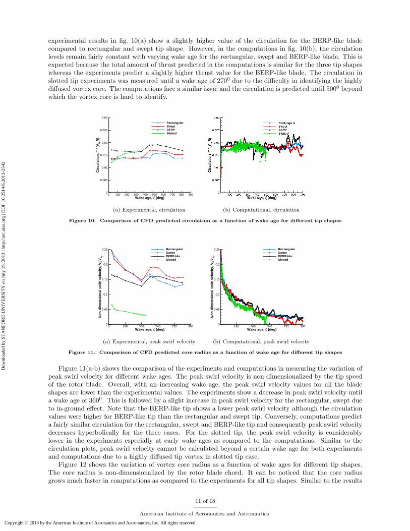
experimental results in fig. 10(a) show a slightly higher value of the circulation for the BERP-like bladecompared to rectangular and swept tip shape. However, in the computations in fig. 10(b), the circulationlevels remain fairly constant with varying wake age for the rectangular, swept and BERP-like blade. This isexpected because the total amount of thrust predicted in the computations is similar for the three tip shapeswhereas the experiments predict a slightly higher thrust value for the BERP-like blade. The circulation inslotted tip experiments was measured until a wake age of 2700 due to the difficulty in identifying the highlydiffused vortex core. The computations face a similar issue and the circulation is predicted until 5000 beyondwhich the vortex core is hard to identify.

Wake age, ζ (deg)

Circ

ulat

ion,

Γ

/ (V

tipR

)

0 100 200 300 400 500 600 700 800 9000

0.005

0.01

0.015

0.02

0.025

0.03

RectangularSweptBERPSlotted

(a) Experimental, circulation (b) Computational, circulation

Figure 10. Comparison of CFD predicted circulation as a function of wake age for different tip shapes

Wake age, ζ (deg)

Non

-dim

ensi

onal

sw

irl v

eloc

ity, V

θ/Vtip

0 180 360 540 720 9000

0.05

0.1

0.15

0.2

0.25 RectangularSweptBERP-likeSlotted

(a) Experimental, peak swirl velocity

Wake age, ζ (deg)

Non

-dim

ensi

onal

sw

irl v

eloc

ity, V

θ/Vtip

180 360 540 720 9000

0.05

0.1

0.15

0.2


(b) Computational, peak swirl velocity

Figure 11. Comparison of CFD predicted core radius as a function of wake age for different tip shapes

Figure 11(a-b) shows the comparison of the experiments and computations in measuring the variation ofpeak swirl velocity for different wake ages. The peak swirl velocity is non-dimensionalized by the tip speedof the rotor blade. Overall, with an increasing wake age, the peak swirl velocity values for all the bladeshapes are lower than the experimental values. The experiments show a decrease in peak swirl velocity untila wake age of 3600. This is followed by a slight increase in peak swirl velocity for the rectangular, swept dueto in-ground effect. Note that the BERP-like tip shows a lower peak swirl velocity although the circulationvalues were higher for BERP-like tip than the rectangular and swept tip. Conversely, computations predicta fairly similar circulation for the rectangular, swept and BERP-like tip and consequently peak swirl velocitydecreases hyperbolically for the three cases. For the slotted tip, the peak swirl velocity is considerablylower in the experiments especially at early wake ages as compared to the computations. Similar to thecirculation plots, peak swirl velocity cannot be calculated beyond a certain wake age for both experimentsand computations due to a highly diffused tip vortex in slotted tip case.

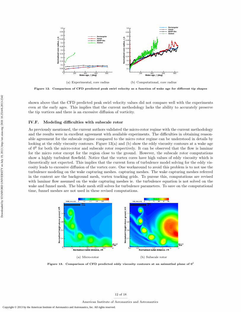
Figure 12 shows the variation of vortex core radius as a function of wake ages for different tip shapes.The core radius is non-dimensionalized by the rotor blade chord. It can be noticed that the core radiusgrows much faster in computations as compared to the experiments for all tip shapes. Similar to the results

11 of 18


Dow

nloa

ded

by S

TA

NFO

RD

UN

IVE

RSI

TY

on

July

19,

201

3 | h

ttp://

arc.

aiaa

.org

| D

OI:

10.

2514

/6.2

013-

2542


Wake age, ζ (deg)

Nor

mal

ized

cor

e ra

dius

, rc/

c

0 200 400 600 8000

0.05

0.1

0.15

0.2

0.25

0.3

0.35

0.4

0.45

0.5

0.55

0.6


(a) Experimental, core radius

Wake age, ζ (deg)

Nor

mal

ized

cor

e ra

dius

, rc/

c

200 400 600 800

0.1

0.15

0.2

0.25

0.3

0.35

0.4

0.45

0.5

0.55


(b) Computational, core radius

Figure 12. Comparison of CFD predicted peak swirl velocity as a function of wake age for different tip shapes

shown above that the CFD predicted peak swirl velocity values did not compare well with the experimentseven at the early ages. This implies that the current methodology lacks the ability to accurately preservethe tip vortices and there is an excessive diffusion of vorticity.

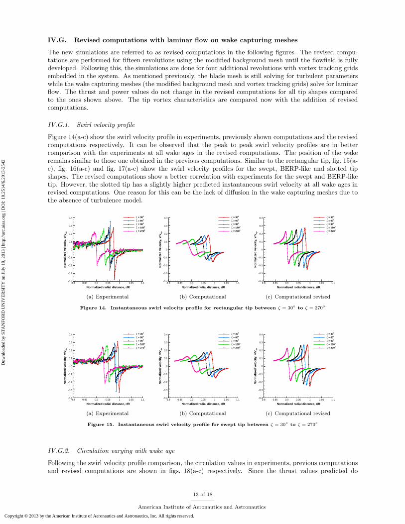
IV.F. Modeling difficulties with subscale rotor

As previously mentioned, the current authors validated the micro-rotor regime with the current methodologyand the results were in excellent agreement with available experiments. The difficulties in obtaining reason-able agreement for the subscale regime compared to the micro rotor regime can be understood in details bylooking at the eddy viscosity contours. Figure 13(a) and (b) show the eddy viscosity contours at a wake ageof 00 for both the micro-rotor and subscale rotor respectively. It can be observed that the flow is laminarfor the micro rotor except for the region close to the ground. However, the subscale rotor computationsshow a highly turbulent flowfield. Notice that the vortex cores have high values of eddy viscosity which istheoretically not expected. This implies that the current form of turbulence model solving for the eddy vis-cosity leads to excessive diffusion of the vortex core. One workaround to avoid this problem is to not use theturbulence modeling on the wake capturing meshes. capturing meshes. The wake capturing meshes referredin the context are the background mesh, vortex tracking grids. To pursue this, computations are revisedwith laminar flow assumed on the wake capturing meshes ie. the turbulence equation is not solved on thewake and funnel mesh. The blade mesh still solves for turbulence parameters. To save on the computationaltime, funnel meshes are not used in these revised computations.

(a) Micro-rotor (b) Subscale rotor

Figure 13. Comparison of CFD predicted eddy viscosity contours at an azimuthal plane of 00

12 of 18


Dow

nloa

ded

by S

TA

NFO

RD

UN

IVE

RSI

TY

on

July

19,

201

3 | h

ttp://

arc.

aiaa

.org

| D

OI:

10.

2514

/6.2

013-

2542


IV.G. Revised computations with laminar flow on wake capturing meshes

The new simulations are referred to as revised computations in the following figures. The revised compu-tations are performed for fifteen revolutions using the modified background mesh until the flowfield is fullydeveloped. Following this, the simulations are done for four additional revolutions with vortex tracking gridsembedded in the system. As mentioned previously, the blade mesh is still solving for turbulent parameterswhile the wake capturing meshes (the modified background mesh and vortex tracking grids) solve for laminarflow. The thrust and power values do not change in the revised computations for all tip shapes comparedto the ones shown above. The tip vortex characteristics are compared now with the addition of revisedcomputations.

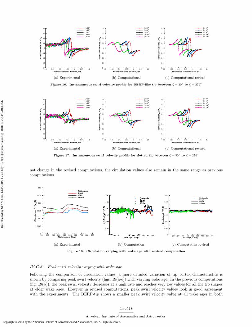
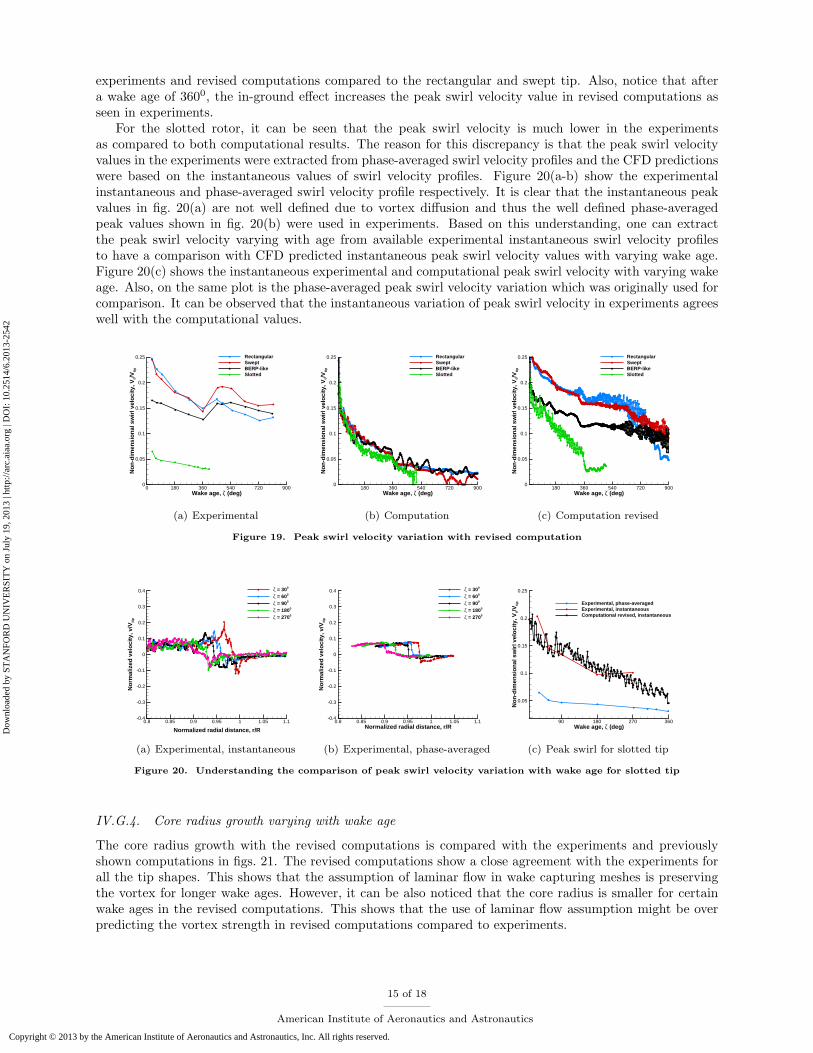
IV.G.1. Swirl velocity profile

Figure 14(a-c) show the swirl velocity profile in experiments, previously shown computations and the revisedcomputations respectively. It can be observed that the peak to peak swirl velocity profiles are in bettercomparison with the experiments at all wake ages in the revised computations. The position of the wakeremains similar to those one obtained in the previous computations. Similar to the rectangular tip, fig. 15(a-c), fig. 16(a-c) and fig. 17(a-c) show the swirl velocity profiles for the swept, BERP-like and slotted tipshapes. The revised computations show a better correlation with experiments for the swept and BERP-liketip. However, the slotted tip has a slightly higher predicted instantaneous swirl velocity at all wake ages inrevised computations. One reason for this can be the lack of diffusion in the wake capturing meshes due tothe absence of turbulence model.


Nor

mal

ized

vel

ocity

, v/V

tip

0.8 0.85 0.9 0.95 1 1.05 1.1-0.4

-0.3

-0.2

-0.1

0

0.1

0.2

0.3

0.4 ζ = 300

ζ = 600

ζ = 900

ζ = 1800

ζ = 2700

(a) Experimental


Nor

mal

ized

vel

ocity

, v/V

tip

0.8 0.85 0.9 0.95 1 1.05 1.1-0.4

-0.3

-0.2

-0.1

0

0.1

0.2

0.3

0.4 ζ = 300

ζ = 600

ζ = 900

ζ = 1800

ζ = 2700

(b) Computational


Nor

mal

ized

vel

ocity

, v/V

tip

0.8 0.85 0.9 0.95 1 1.05 1.1-0.4

-0.3

-0.2

-0.1

0

0.1

0.2

0.3

0.4 ζ = 300

ζ = 600

ζ = 900

ζ = 1800

ζ = 2700

(c) Computational revised

Figure 14. Instantaneous swirl velocity profile for rectangular tip between ζ = 30◦ to ζ = 270◦


Nor

mal

ized

vel

ocity

, v/V

tip

0.8 0.85 0.9 0.95 1 1.05 1.1-0.4

-0.3

-0.2

-0.1

0

0.1

0.2

0.3

0.4 ζ = 300

ζ = 600

ζ = 900

ζ = 1800

ζ = 2700

(a) Experimental


Nor

mal

ized

vel

ocity

, v/V

tip

0.8 0.85 0.9 0.95 1 1.05 1.1-0.4

-0.3

-0.2

-0.1

0

0.1

0.2

0.3

0.4 ζ = 300

ζ = 600

ζ = 900

ζ = 1800

ζ = 2700

(b) Computational


Nor

mal

ized

vel

ocity

, v/V

tip

0.8 0.85 0.9 0.95 1 1.05 1.1-0.4

-0.3

-0.2

-0.1

0

0.1

0.2

0.3

0.4 ζ = 300

ζ = 600

ζ = 900

ζ = 1800

ζ = 2700


Figure 15. Instantaneous swirl velocity profile for swept tip between ζ = 30◦ to ζ = 270◦

IV.G.2. Circulation varying with wake age

Following the swirl velocity profile comparison, the circulation values in experiments, previous computationsand revised computations are shown in figs. 18(a-c) respectively. Since the thrust values predicted do

13 of 18


Dow

nloa

ded

by S

TA

NFO

RD

UN

IVE

RSI

TY

on

July

19,

201

3 | h

ttp://

arc.

aiaa

.org

| D

OI:

10.

2514

/6.2

013-

2542



Nor

mal

ized

vel

ocity

, v/V

tip

0.8 0.85 0.9 0.95 1 1.05 1.1-0.4

-0.3

-0.2

-0.1

0

0.1

0.2

0.3

0.4 ζ = 300

ζ = 600

ζ = 900

ζ = 1800

ζ = 2700

(a) Experimental


Nor

mal

ized

vel

ocity

, v/V

tip

0.8 0.85 0.9 0.95 1 1.05 1.1-0.4

-0.3

-0.2

-0.1

0

0.1

0.2

0.3

0.4 ζ = 300

ζ = 600

ζ = 900

ζ = 1800

ζ = 2700

(b) Computational


Nor

mal

ized

vel

ocity

, v/V

tip

0.8 0.85 0.9 0.95 1 1.05 1.1-0.4

-0.3

-0.2

-0.1

0

0.1

0.2

0.3

0.4 ζ = 300

ζ = 600

ζ = 900

ζ = 1800

ζ = 2700


Figure 16. Instantaneous swirl velocity profile for BERP-like tip between ζ = 30◦ to ζ = 270◦


Nor

mal

ized

vel

ocity

, v/V

tip

0.8 0.85 0.9 0.95 1 1.05 1.1-0.4

-0.3

-0.2

-0.1

0

0.1

0.2

0.3

0.4 ζ = 300

ζ = 600

ζ = 900

ζ = 1800

ζ = 2700

(a) Experimental


Nor

mal

ized

vel

ocity

, v/V

tip

0.8 0.85 0.9 0.95 1 1.05 1.1-0.4

-0.3

-0.2

-0.1

0

0.1

0.2

0.3

0.4 ζ = 300

ζ = 600

ζ = 900

ζ = 1800

ζ = 2700

(b) Computational


Nor

mal

ized

vel

ocity

, v/V

tip

0.8 0.85 0.9 0.95 1 1.05 1.1-0.4

-0.3

-0.2

-0.1

0

0.1

0.2

0.3

0.4 ζ = 300

ζ = 600

ζ = 900

ζ = 1800

ζ = 2700


Figure 17. Instantaneous swirl velocity profile for slotted tip between ζ = 30◦ to ζ = 270◦

not change in the revised computations, the circulation values also remain in the same range as previouscomputations.

Wake age, ζ (deg)

Circ

ulat

ion,

Γ

/ (V

tipR

)

0 100 200 300 400 500 600 700 800 9000

0.005

0.01

0.015

0.02

0.025

0.03


(a) Experimental (b) Computation

Wake age, ζ (deg)

Circ

ulat

ion,

Γ

/ (V

tipR

)

100 200 300 400 500 600 700 800 9000

0.005

0.01

0.015

0.02

0.025

0.03


(c) Computation revised

Figure 18. Circulation varying with wake age with revised computation

IV.G.3. Peak swirl velocity varying with wake age

Following the comparison of circulation values, a more detailed variation of tip vortex characteristics isshown by comparing peak swirl velocity (figs. 19(a-c)) with varying wake age. In the previous computations(fig. 19(b)), the peak swirl velocity decreases at a high rate and reaches very low values for all the tip shapesat older wake ages. However in revised computations, peak swirl velocity values look in good agreementwith the experiments. The BERP-tip shows a smaller peak swirl velocity value at all wake ages in both

14 of 18


Dow

nloa

ded

by S

TA

NFO

RD

UN

IVE

RSI

TY

on

July

19,

201

3 | h

ttp://

arc.

aiaa

.org

| D

OI:

10.

2514

/6.2

013-

2542


experiments and revised computations compared to the rectangular and swept tip. Also, notice that aftera wake age of 3600, the in-ground effect increases the peak swirl velocity value in revised computations asseen in experiments.

For the slotted rotor, it can be seen that the peak swirl velocity is much lower in the experimentsas compared to both computational results. The reason for this discrepancy is that the peak swirl velocityvalues in the experiments were extracted from phase-averaged swirl velocity profiles and the CFD predictionswere based on the instantaneous values of swirl velocity profiles. Figure 20(a-b) show the experimentalinstantaneous and phase-averaged swirl velocity profile respectively. It is clear that the instantaneous peakvalues in fig. 20(a) are not well defined due to vortex diffusion and thus the well defined phase-averagedpeak values shown in fig. 20(b) were used in experiments. Based on this understanding, one can extractthe peak swirl velocity varying with age from available experimental instantaneous swirl velocity profilesto have a comparison with CFD predicted instantaneous peak swirl velocity values with varying wake age.Figure 20(c) shows the instantaneous experimental and computational peak swirl velocity with varying wakeage. Also, on the same plot is the phase-averaged peak swirl velocity variation which was originally used forcomparison. It can be observed that the instantaneous variation of peak swirl velocity in experiments agreeswell with the computational values.

Wake age, ζ (deg)

Non

-dim

ensi

onal

sw

irl v

eloc

ity, V

θ/Vtip

0 180 360 540 720 9000

0.05

0.1

0.15

0.2


(a) Experimental

Wake age, ζ (deg)

Non

-dim

ensi

onal

sw

irl v

eloc

ity, V

θ/Vtip

180 360 540 720 9000

0.05

0.1

0.15

0.2


(b) Computation

Wake age, ζ (deg)

Non

-dim

ensi

onal

sw

irl v

eloc

ity, V

θ/Vtip

180 360 540 720 9000

0.05

0.1

0.15

0.2



Figure 19. Peak swirl velocity variation with revised computation


Nor

mal

ized

vel

ocity

, v/V

tip

0.8 0.85 0.9 0.95 1 1.05 1.1-0.4

-0.3

-0.2

-0.1

0

0.1

0.2

0.3

0.4 ζ = 300

ζ = 600

ζ = 900

ζ = 1800

ζ = 2700

(a) Experimental, instantaneous


Nor

mal

ized

vel

ocity

, v/V

tip

0.8 0.85 0.9 0.95 1 1.05 1.1-0.4

-0.3

-0.2

-0.1

0

0.1

0.2

0.3

0.4 ζ = 300

ζ = 600

ζ = 900

ζ = 1800

ζ = 2700

(b) Experimental, phase-averaged

Wake age, ζ (deg)

Non

-dim

ensi

onal

sw

irl v

eloc

ity, V

θ/Vtip

90 180 270 360

0.05

0.1

0.15

0.2

0.25

Experimental, phase-averagedExperimental, instantaneousComputational revised, instantaneous

(c) Peak swirl for slotted tip

Figure 20. Understanding the comparison of peak swirl velocity variation with wake age for slotted tip

IV.G.4. Core radius growth varying with wake age

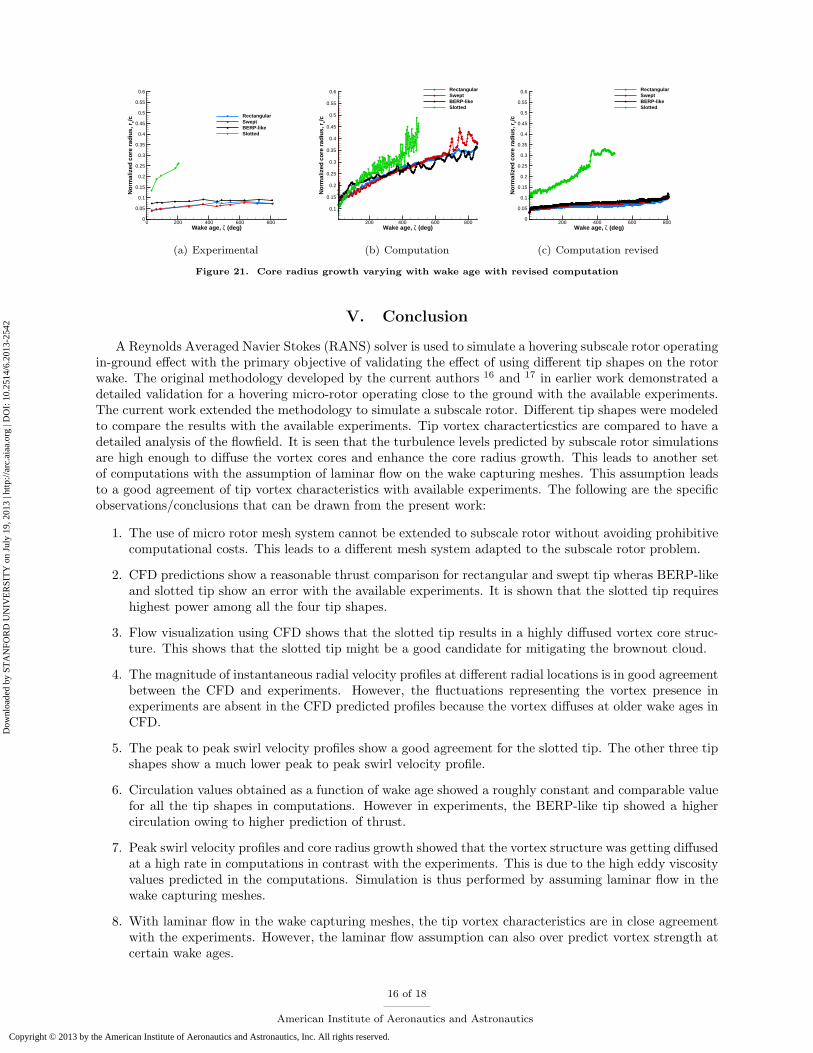
The core radius growth with the revised computations is compared with the experiments and previouslyshown computations in figs. 21. The revised computations show a close agreement with the experiments forall the tip shapes. This shows that the assumption of laminar flow in wake capturing meshes is preservingthe vortex for longer wake ages. However, it can be also noticed that the core radius is smaller for certainwake ages in the revised computations. This shows that the use of laminar flow assumption might be overpredicting the vortex strength in revised computations compared to experiments.

15 of 18


Dow

nloa

ded

by S

TA

NFO

RD

UN

IVE

RSI

TY

on

July

19,

201

3 | h

ttp://

arc.

aiaa

.org

| D

OI:

10.

2514

/6.2

013-

2542


Wake age, ζ (deg)

Nor

mal

ized

cor

e ra

dius

, rc/

c

0 200 400 600 8000

0.05

0.1

0.15

0.2

0.25

0.3

0.35

0.4

0.45

0.5

0.55

0.6


(a) Experimental

Wake age, ζ (deg)

Nor

mal

ized

cor

e ra

dius

, rc/

c

200 400 600 800

0.1

0.15

0.2

0.25

0.3

0.35

0.4

0.45

0.5

0.55


(b) Computation

Wake age, ζ (deg)

Nor

mal

ized

cor

e ra

dius

, rc/

c

200 400 600 8000

0.05

0.1

0.15

0.2

0.25

0.3

0.35

0.4

0.45

0.5

0.55



Figure 21. Core radius growth varying with wake age with revised computation

V. Conclusion

A Reynolds Averaged Navier Stokes (RANS) solver is used to simulate a hovering subscale rotor operatingin-ground effect with the primary objective of validating the effect of using different tip shapes on the rotorwake. The original methodology developed by the current authors 16 and 17 in earlier work demonstrated adetailed validation for a hovering micro-rotor operating close to the ground with the available experiments.The current work extended the methodology to simulate a subscale rotor. Different tip shapes were modeledto compare the results with the available experiments. Tip vortex characterticstics are compared to have adetailed analysis of the flowfield. It is seen that the turbulence levels predicted by subscale rotor simulationsare high enough to diffuse the vortex cores and enhance the core radius growth. This leads to another setof computations with the assumption of laminar flow on the wake capturing meshes. This assumption leadsto a good agreement of tip vortex characteristics with available experiments. The following are the specificobservations/conclusions that can be drawn from the present work:

1. The use of micro rotor mesh system cannot be extended to subscale rotor without avoiding prohibitivecomputational costs. This leads to a different mesh system adapted to the subscale rotor problem.

2. CFD predictions show a reasonable thrust comparison for rectangular and swept tip wheras BERP-likeand slotted tip show an error with the available experiments. It is shown that the slotted tip requireshighest power among all the four tip shapes.

3. Flow visualization using CFD shows that the slotted tip results in a highly diffused vortex core struc-ture. This shows that the slotted tip might be a good candidate for mitigating the brownout cloud.

4. The magnitude of instantaneous radial velocity profiles at different radial locations is in good agreementbetween the CFD and experiments. However, the fluctuations representing the vortex presence inexperiments are absent in the CFD predicted profiles because the vortex diffuses at older wake ages inCFD.

5. The peak to peak swirl velocity profiles show a good agreement for the slotted tip. The other three tipshapes show a much lower peak to peak swirl velocity profile.

6. Circulation values obtained as a function of wake age showed a roughly constant and comparable valuefor all the tip shapes in computations. However in experiments, the BERP-like tip showed a highercirculation owing to higher prediction of thrust.

7. Peak swirl velocity profiles and core radius growth showed that the vortex structure was getting diffusedat a high rate in computations in contrast with the experiments. This is due to the high eddy viscosityvalues predicted in the computations. Simulation is thus performed by assuming laminar flow in thewake capturing meshes.

8. With laminar flow in the wake capturing meshes, the tip vortex characteristics are in close agreementwith the experiments. However, the laminar flow assumption can also over predict vortex strength atcertain wake ages.

16 of 18


Dow

nloa

ded

by S

TA

NFO

RD

UN

IVE

RSI

TY

on

July

19,

201

3 | h

ttp://

arc.

aiaa

.org

| D

OI:

10.

2514

/6.2

013-

2542


The current work compared the RANS based predictions for a subscale rotor with different tip shapeswith available experiments. The high eddy viscosity values in the vortex cores indicated that the current formof turbulence model is leading to excessive diffusion of vorticity. Consequently, the laminar flow assumptionon wake capturing meshes leads to a good agreement of tip vortex characteristics between the experimentsand computations. Since it is essential to capture the turbulence on the ground for understanding brownoutphenomenon, future work needs to investigate and improve the current formulation of turbulence model.

Acknowledgments

”The Air Force Office of Scientific Research supported this work under a Multidisciplinary UniversityResearch Initiative, Grant W911NF0410176. The contract monitor was Dr. Douglas Smith. The work onthe vortex tracking grids was supported by NAVAIR at Pax River, with Dr. Yik-Loon Lee as the technicalmonitor. The authors wish to thank all of their colleagues at the University of Maryland, Governmentresearch labs, and the rotorcraft industry for the valuable discussions on the brownout problem.”

References

1Lee, T. E., Leishman, J. G., and Ramasamy, M., “Fluid Dynamics of Interacting Blade Tip Vortices With a GroundPlane,” American Helicopter Society 64th Annual Forum Proceedings, Montr’eal, Canada, April 29–May 1, 2008.

2Milluzzo, J., Sydney, A., Rauleder, J., Leishman, J. G., “In Ground Effect Aerodynamics of Rotors with Different BladeTips,”, American Helicopter Society 66th Annual Forum Proceedings, Phoenix, AZ, May 11–13,2010.

3Hance, B.T., “Effects of Body Shapes on Rotor In-Ground-Effect Aerodynamics,” Masters. theses, Department ofAerospace Engineering, University of Maryland at College Park, 2012.

4Johnson, B., Leishman, J. G., and Sydney, A., “Investigation of Sediment Entrainment in Brownout Using High-SpeedParticle Image Velocimetry,” American Helicopter Society 65th Annual Forum Proceedings, , Grapevine, TX, May 27–29, 2009.

5Sydney, A., Baharani, A., Leishman, J.G., “Understanding Brownout Conditions from Dual-Phase Flow Measurements ofDust Uplift Mechanisms,” American Helicopter Society 67th Annual Forum Proceedings, Virginia Beach, VA, May 3–5,2010.

6Nathan, N.D., and Green, R.B., “Measurements of a rotor flow in ground effect and visualization of the brown-outphenomenon,” American Helicopter Society 64th Annual Forum Proceedings, Montr’eal, Canada, April 29–May 1, 2008.

7Syal, M., Govindarajan, B., and Leishman, J. G., “Mesoscale Sediment Tracking Methodology to Analyze Brownout CloudDevelopments,” Proceedings of the 66th Annual American Helicopter Society Forum, Phoenix, AZ, May 11–14, 2010.

8Syal, M., and Leishman, J. G., “Comparisons of Predicted Brownout Dust Clouds with Photogrammetry Measurements,”Proceedings of the 67th Annual American Helicopter Society Forum, Virginia Beach, VA, May 3–5, 2011.

9Wachspress, D.A., Whitehouse, G.R., Keller, J.D., , Yu, K., Gilmore, P., Dorsett, M., McClure, K.,“High Fidelity RotorAerodynamic Module for Real Time Rotorcraft Flight Simulation,”AIAA Journal, Vol. 38, (1), 2000, pp. 5763.

10Brown, R. E.,“Rotor Wake Modeling for Flight Dynamic Simulation of Helicopters, ”AIAA Journal, Vol. 38, (1), 2000,pp. 5763.

11Brown, R. E. and Line, A. J.,“Efficient High-Resolution Wake Modeling using the Vorticity Transport Equation,”AIAA

Journal, Vol. 43, (7), 2005, pp. 1434-144312Phillips, C., and Brown, R.E., “Eulerian Simulation of the Fluid Dynamics of Helicopter Brownout,” American Helicopter

Society 64th Annual Forum Proceedings, Montr’eal, Canada, April 29–May 1, 2008.13Hu, G., Grossman, B., and Steinhoff, J., “Numerical Method for Vorticity Confinement in Compressible Flow,” AIAA

Journal, Vol. 40, (10), 2002, pp. 1945-1953.14Haehnel, R. B., Moulton, M. A., Wenren, W., and Steinhoff, J., “A Model to Simulate Rotorcraft-Induced Brownout,”

American Helicopter Society 64th Annual Forum Proceedings, Montr’eal, Canada, April 29–May 1, 2008.15Thomas, S., and Baeder J.D.,“A Hybrid CFD Methodology to Model the Two-phase Flowfield beneath a Hovering

Laboratory Scale Rotor,” 30th AIAA Applied Aerodynamics Conference, New Orleans, LA, June 25–28, 2012.16Kalra T.S., Lakshminarayan V.K., Baeder J.D., “CFD Validation of Micro Hovering Rotor in Ground Effect , American

Helicopter Society 66th Annual Forum Proceedings, Phoenix, Az, May 11–13, 2010.17Kalra T.S., Lakshminarayan V.K., Baeder J.D., and Thomas, S., “CFD Validation Methodological Improvements for

Computational Study of Hovering Micro-Rotor in Ground Effect,” 20th AIAA Computational Fluid Dynamics Conference,Honolulu, Hi, June 27–30, 2011.

18Lakshminarayan, V. K., “Computational Investigation of Micro-Scale Coaxial Rotor Aerodynamics in Hover,” Ph.D.dissertation, Department of Aerospace Engineering, University of Maryland at College Park, 2009.

19Buelow P. E. O., Schwer D. A., Feng J., and Merkle C. L. “A Preconditioned Dual-Time, Diagonalized ADI scheme forUnsteady Computations,” AIAA paper 1997-2101, 13th AIAA Computational Fluid Dynamics Conference, Snowmass Village,CO, June 29–July 2, 1997.

20Pandya, S. A., Venkateswaran, S., and Pulliam, T. H. “Implementation of Preconditioned Dual-Time Procedures inOVERFLOW,” AIAA paper 2003-0072, 41st AIAA Aerospace Sciences Meeting and Exhibit, Reno, NV, January 6–9, 2003.

21Pulliam, T., and Chaussee, D., “A Diagonal Form of an Implicit Approximate Factorization Algorithm,” Journal of

Computational Physics, Vol. 39, (2), February 1981, pp. 347–363. Fluid Dynamics,” Annual Review of Fluid Mechanics,

Vol. 31, January 1999, pp. 385–416.

17 of 18


Dow

nloa

ded

by S

TA

NFO

RD

UN

IVE

RSI

TY

on

July

19,

201

3 | h

ttp://

arc.

aiaa

.org

| D

OI:

10.

2514

/6.2

013-

2542


22Turkel, E., Preconditioning Techniques in Computational Fluid Dynamics, Annual Review of Fluid Mechanics , Vol. 31,January 1999, pp. 385- 416.

23Van Leer B., “Towards the Ultimate Conservative Difference Scheme V. A Second-Order Sequel To Godunovs Method,Journal of Computational Physics, Vol. 135, No. 2, 1997, pp. 229-248.

24Koren B., “Upwind Schemes, Multigrid and Defect Correction for the Steady Navier-Stokes Equations, 11th InternationalConference on Numerical Methods in Fluid Dynamics, Willamsburg, VA, June 1988

25Henrick, A. K., Aslam, T. D., and Powers, J. M., “Mapped Weighted Essentially Non-oscillatory Schemes: AchievingOptimal Order Near Critical Points,” Journal of Computational Physics, Vol. 207, No. 2, 2005, pp. 542–567.

26Roe, P., “Approximate Riemann Solvers, Parameter Vectors and Difference Schemes,” Journal of Computational Physics,Vol. 135, No. 2, 1997, pp. 250-258.

27Spalart, P. R., and Allmaras, S. R., “A One-equation Turbulence Model for Aerodynamic Flows,” AIAA Paper 1992-0439,30th AIAA Aerospace Sciences Meeting and Exhibit, Reno, NV, January 6–9, 1992.

28Duraisamy, K., “Studies in Tip Vortex Formation, Evolution and Control,” Ph.D. Dissertation, Department of AerospaceEngineering, University of Maryland at College Park, 2005.

29Lee, Y., “On Overset Grids Connectivity and Automated Vortex Tracking in Rotorcraft CFD,” Ph.D. Dissertation,Department of Aerospace Engineering, University of Maryland, College Park, 2008.

30Jeong, J., and Hussain, F., “On the Identification of a Vortex,” Journal of Fluid Mechanics, Vol. 285, 1995, pp. 69–94.

18 of 18


Dow

nloa

ded

by S

TA

NFO

RD

UN

IVE

RSI

TY

on

July

19,

201

3 | h

ttp://

arc.

aiaa

.org

| D

OI:

10.

2514

/6.2

013-

2542


Effect of Tip Geometry on a Hovering Rotor in Ground ... · Eﬀect of Tip Geometry on a Hovering...

Documents

Transcript of Effect of Tip Geometry on a Hovering Rotor in Ground ... · Eﬀect of Tip Geometry on a Hovering...