
![RADIO-FREQUENCY AMPLIFIERS. - NIST Pagenvlpubs.nist.gov/nistpubs/ScientificPapers/nbsscientificpaper449... · Lowell] Radio-FrequencyAmplifiers. 337 iscoupledtotheinputorgridcircuitofthenexttubebyanyone](https://static.fdocuments.us/doc/165x107/5a79ffef7f8b9a71348b7882/radio-frequency-amplifiers-nist-radio-frequencyamplifiers-337-iscoupledtotheinputorgridcircuitofthenexttubebyanyone.jpg)


Languages
Pages
Legal


ADJUSTMENT OF PARABOLIC AND LINEAR CURVESTO OBSERVATIONS TAKEN AT EQUAL INTERVALSOF THE INDEPENDENT VARIABLE
By Harry M. Roeser
Perhaps the two formulas which have the widest utility in
the representation of the variation between two mutually depen-
dent physical quantities X and Y are
Y=A+BX +CX 2 (i)
and Y =A+BX (2)
The best or most probable values of the constants A, B, and
C of equation (1), or A and B of equation (2) can only be deter-
mined by the method of least squares, which involves consider-
able computation, apparently superficial, and often too excessive
to warrant the application of that method. Recourse is often
had to various graphical or empirical methods. These usually
depend upon the skill of the experimenter in placing a line byeye, or the arbitrary selection of certain of the observations as
having undue weight, and consequently the values obtained
bear the defect of personal judgment. A reduction, either
sufficiently approximate or absolutely correct, of the method of
least squares to utilitarian convenience is therefore desirable.
The author purposes to develop a scheme which leaves the
method of least squares without approximation as far as its
application in many special cases to forms (1) and (2) is con-
cerned. By following this scheme the major portion of the
quantities involved in the mathematical expressions for the
constants can be written down at once from inspection of the
observations or consulting Table 5 accompanying the paper.
The mathematical processes consist of the most fundamental
arithmetic operations.
The proposed scheme depends upon the simple expedient of
taking observations of Y at equal intervals of X. This is quite
generally done in practice either involuntarily or to secure a
desired continuity in a graphical representation. In such routine
181030°—20 363
364 Scientific Papers of the Bureau of Standards [Vol. 16
practice where least-square solutions are necessary, the proposed
scheme apparently has limited application on account of the
requirement that observations be taken at equal intervals of the
independent variable. However, the tedious arithmetical labor
of making the regular solutions is conspicuously reduced with
no ensuing loss in accuracy. Adapting the collection of routine
data to the conditions to which the scheme applies will generally
be found practicable and advantageous.
The method in its utmost simplicity applies to observations of
equal weight, although by following the general plan the reduction
of observations of unequal weight can be greatly expedited. Theanalytical development is unessential to the practical application.
All necessary definitions and formulas are given in connection
with Table 5.
1. SOLUTION FOR Y=A+BX+CX2
Consider observations that fall along a curve of type (1).
The normal equations which are set up by the method of least
squares to determine <he most probable values of A, B, and Cfrom more than three observations are
—
nA+BVX +CVX 2 =2YA2X+BXX 2 +C2X *=XXY (3)
where n is the number of observations.
The general objection that the labor involved in a least-square
solution is excessive is forced upon the mind by a consideration of
equations (3) , especially if n is a large number and the X's contain
three or more significant figures. Aside from the labor of setting
up the normal equations that of merely solving them when the
coefficients are large is considerable.
Let the center of coordinates be transferred to the point
(Xm , Ym), and in the new system let equation (1) change to
y = a 4- bx + ex2(4)
that is, let y = Y — Ym , and x =X -Xm
Then, as becomes apparent from simple substitution of these
values and reduction,
A = Ym +a-Xm (b-cXm) (5)
B=b-2cXm (6)
C=c (7)

Roeser] Adjustment of Curves to Observations, Etc. 365
in which a, b, and c remain to be determined. Equations (3)
reduce to
—
na + bXx + cZx2 =zZy
a2x + b2x2 + c?;x3 =2xy > (8)
dZx2 + bXx3 + cZx4 = Hx2y .
Now it is a well-known property of the arithmetic mean of a
set of values, that the summation of the odd powers of differences
or "deviations" of the values from the arithmetic mean is zero.
Therefore in equations (8), Xx, Sy, and 2x3 are zero, since x and yare, respectively, measured from the mean values of X and Y.
After dividing each of equations (8) by n, they reduce to
—
a
2x2
n
cZx2
n=
bXx2 JZxyn n
c2x4 2x2
yn n
(9)
. If the observations are taken at equal intervals of X, equations
(9) may be further simplified by taking advantage of the fact that
H1X2 2x4— and — may be made independent of x.
n n J r
Let i be the interval between successive values of X. Then
—
(n-i) .X x=Xm .1 ; or , x
x
-A. 9 — -A- m 1 >l
,
X3 —X 1
2
(n ~ 5)
3.1;
x (j^3l.i
&,= ^-.i
n-J^n-ti n-(2n-s) .
^(n-l) —^m ~»5:> OI
> *(n-l)= "
•*
^r ^ n — (2n — i) . n — {2n—\) .
J\. n =JL m .i\ or, xn = .1
Therefore
Xtf^j2
n 4n|
and
n
(n-i) 2 + (n-3) 2 + (n-5) 2 + • • + {n- (2»- i)} 21 (10)
4i4 r ~i
- = ^[(^-i) 4 +(^-3) 4 +(^-5) 4 + ' • ' +{n-(2n-i)y\ (11)

366 Scientific Papers of the Bureau of Standards [vd. 16
After summing the terms within the brackets, (10) and (n),
reduce to
—
— =—(n — i)(n + i)n i2
v (12)
— = (n - i) (n + i) (^n2 - j)n 240v y J " (13)
The right-hand members of (12) and (13) are independent of x.
Write now
— (n — 1) (n + i) =i2u12
(14)
t4
i2— (w-j-i) (w + i) ($ri -j) =iH = —(3Yi2 -i)u (15)
Equations (9) thus reduce to
a
i2ub
ilua + i*vc =
+ i2uc = o
Xxy
n
n J
(16)
These equations yield for the required values of a, b, and c,
1 2x2y uv n u2 — v
Let
Then
b = ^r-Xi 'Zxy
-u n
_ a
i2u
o = y =— ,
-—— =20.» n v—vr
T'wa= —
6 = -^ X-
a 1
i2 w
(17)
(18)
(19)
(20)
(21)
(22)

Roeser] Adjustment of Curves to Observations, Etc. 367
For convenience in writing down the solutions values of w and
- are tabulated in Table 5 for values of n from 5 to 31.
The computation of S' and T' from the observations on X and
Y will be greatly facilitated by use of the results obtained from
the following considerations:
s,j:xyJ2{X-Xm)(Y-Ym) _
n n
Arrange the constituent parts of the summation in pairs as
follows: (1) First and last, (2) second and next to the last, (3) third
and third from the last, etc., thus:
ix*-xm ) (y1-ym) = -i^^(y1-Ym)
(xn-xm) (yn-ym) = -^~ (2
2
n " l)(Y:n-ym)
(X2-Xm)(Y2 -Yrn) = -i^^(Y2-Ym)
(Xn_ 1-Xm)(Yn- 1-Ym) = -i
n ~ (2"~ 3) (Y^ 1-Ym)
, etc.
Now collect terms in the pairs of expressions connected bybrackets ; there results
:
S'=^ = ^[(n-i)(Yn-Y l) + (n- 3)(Yn- l-Y1)+---]=iS(23)
Similarly for T'
n 2n
nArrange the observations in pairs
:
(X.-X^iY,- Ym) =i2
(^-11J(Y1-Ym)
(X2-Xm)(Y2- Ym)
=*^iz3j(y1_ Ym)
etc.

368 Scientific Papers of the Bureau of Standards [vol. 16
Therefore,
-^2yJ (n-i) 2 + (n- 3 )2 + • • •
-J
= ^[(n-i) 2(ri + ym) +(n- 3 )
2(y2 + Yn_ 1) + • • • ]-*Wm
(24)
(25)
(26)
(27)
These last equations serve to determine completely the values
of A, B, and C, according to equations (5), (6), and (7).
To save mental effort in the summations, values are furnished
in Table 5 for the squares of the terms containing n. Thus if n is
an even number, say 18, (n-1) 2is given in the table opposite 18;
(rc-3) 2is the next preceding tabular value in that column; (n-5) 2
is the second preceding value, and so forth. The arrangement is
similar for n, an odd number.
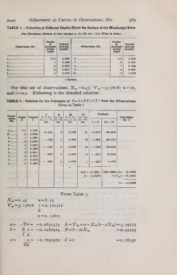
A numerical example of the application of the above to a prac-
tical problem will now be given. Consider the problem of deter-
mining the depth-velocity curve discussed on page 131 of Merri-
man's "Method of Least Squares," eighth edition ; 191 3, Wiley &Sons. The original data give observations on the velocity of
flow of the Mississippi River at different percentages of the total
depth. The values of velocity Y, plotted against depth X, follow
closely a smooth curve whose equation is assumed to be Y = A +BX +CX2
. It is required to determine the most probable values
of A, B, and C from the observations. The observations follow:
= i2T
Equations (20), (21), and {1\2) then reduce to
»
a— —Tw
l u
a
i2u
Adjustment of Curves to Observations, Etc.Roeser) Adjustment oj curves to uoservations, tLtc. 369
TABLE 1.—Velocities at Different Depths Below the Surface of the Mississippi River
[See Merriman, Method of least squares, p. 131, 8th ed.; 1913, Wiley & Sons.]
Observation No.
Depthsin
decimalsof total
depth
Velocity(feet persecond)
Observation No.
Depthsin
decimalsof total
depth
Velocity(feet persecond)
1 ' aO.O
.1
.2
.3
.4
3. 1950
3. 2299
3. 2532
3. 2611
3. 2516
6 0.5
.6
.7
.8
.9
3. 2282
2 7 3 1807
3 .. 8 3 1266
4 9 3 0594
5 10 2. 9759
a Surface.
For this set of observations, Xm = o.45; 1^ = 3.17616; n=io,and i — o. 1 . Following is the detailed solution
:
TABLE 2.—Solution for the Constants of Y=A+BX+CX 2 from the Observations
Given in Table 1
Obser- DepthX
VelocityY
I
Yn-YnYn-l- Yi,
etc.
II
(n-1),(»-3),
etc.
mYn+ YuYa-l+ Y2,
etc.
IV(n-l)«,(«-3)2,
etc.
Products
CalculationvationNo.
I XII inx ivfor T
1.*....
10
0.0
.9
3. 1950
2. 9759 }
-0. 2191 9 6. 1709 81 -1.9719 499. 8429
2
9
.1
.8
3. 2299
3. 0594 }
- .1705 7 6. 2893 49 -1. 1935 308. 1757
3
8
.2
.7
3. 2532
3. 1266 }
- .1266 5 6. 3798 25 - .6330 159. 4950
4
7
.3
.6
3.2611
3. 1807 }
- .0804 3 6.4418 9 - .2412 57. 9762
5
6
.4
.5
3. 2516
3. 2282 }
- .0234 1 6. 4798 1 - .0234 6. 4798
2nS= -4. 0630 1031. 9696-r 4n= 25. 79924
S= -0.20315 -ulfm= -26. 20332
T= -0.40408
From Table 5
Xm =o.45 ^ = 8.25
3^1 = 3.17616 1=0.121212u
w = o. 15625
a= -Tw= +0.0631375 A = Ym +a-Xm(b-cXm) =3. 19513b= S t= — o. 2462424 B = b — 2cXm =0.44253
i uc= — a= -0.7652970 C=c =0.76530

37° Scientific Papers of the Bureau of Standards [Vol. 16
Therefore Y = 3 - 19513 +0. 44523X-0. 76530X2.
This checks exactly with the equation given by Merriman.
2. SOLUTION FOR Y=A+BX.
The normal equations which yield the most probable values of
A and B from n observations of equal weight ofX and Y are,
nA+BXX =27 1
A.XX+BXX2 =2X7J
(28)
If the observations are taken at equal intervals of X and after
plotting in a system of rectangular coordinates the center of
coordinates be transferred to X,Y =Xm,Ym , equations (28)
reduce to,
n. a.
bXx2 = i:xyZxy\ <2*>
in which x =X —Xm and Y = Ym
Therefore, a=o (30)
Hxy 5 1
b =Xx^ = 7u <?',}
in which u is defined as in equation (14) and 5 as in equation (23).
In the old system of coordinates whose center is at X, Y = 0, o
B=b (32)
A = Ym -bXm (33)
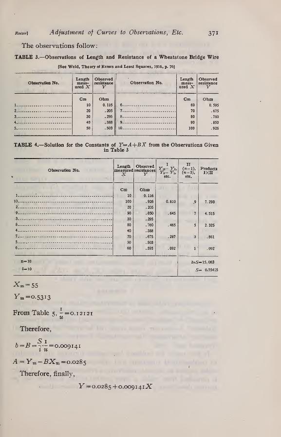
As an example of the practical application of the above, a
solution is given of a problem adapted from page 74, Weld, Theory
of Errors and Least Squares, 19 16 (MacMillan).
To measure the total resistance of a Wheatstone bridge wire
and to calibrate the wire at the same time are desired. The
wire is 100 cm long. The resistance was measured of the first
10 cm, then of the first 20 cm, etc., and finally of the whole wire.
The resistance of the connections entered each time as a constant
term in the above resistances.
Let A be the resistance of the connections, B the unit resistance
of the bridge wire, X the length of wire for which the resistance
was observed, and Y the observed resistance; then,
Y=A+BX
Roeser] Adjustment of Curves to Observations, Etc. 371
The observations follow:
TABLE 3.—Observations of Length and Resistance of a Wheatstone Bridge Wire
[See Weld, Theory of Errors and Least Squares, 1916, p. 76]
Observation No.Lengthmeas-ured X
Observedresistance
YObservation No.
Lengthmeas-
ured XObservedresistance
Y
1
Cm10
20
30
40
50
Ohm0.116
.205
.295
.388
.503
6
Cm60
70
80
90
100
Ohm595
2 7 .675
3 8 760
4 9 850
5 10 926
TABLE 4.—Solution for the Constants of Y=A+BX from the Observations Givenin Table 3
Observation No.
>
LengthmeasuredX
Observedresistances
Y
I
Yio- Yi,Y9- Y2 ,
etc.
II
(rc-D,(»-3),etc.
ProductsIXII
1
Cm10
100
20
90
30
80
40
70
50
60
Ohm0.116
.926
.205
.850
.295
.760
.388
.675
.503
.595
0.810
.645
.465
.287
.092
.9
7
5
3
1
10 7.290
2.
9 4.515
3
8 2.325
4
7 .861
5
6 .092
n=10
i=10
2kS=15.083
S= 0.75415
Vr
m =o.53i3
From Table 5, - = 0.12121u
Therefore,
b=B = -—= 0.0091411 u
A = Ym -BXm = 0.0285
Therefore, finally,
Y =0.0285 +0.009141X

372 Scientific Papers of the Bureau of Standards [Voi.16
This equation is not the same as that obtained by Weld. There
is an error in his solution. The least-square solution gives values
for the constants which check with the above.
3. SOLUTION WHEN A OR B OR BOTH A AND B ARE ZERO.
Should any of the constants A, B, and C be zero, that is, if
the curve to be fitted to the observations is of one of the follow-
ing forms
—
V =CX2(34)
Y=BX + CX> (35)
Y=A+CX> (36)
Y=BX (37)
the solutions given above for the constants do not hold. Such
curves are constrained to fulfill certain geometric conditions
independent of the observations themselves; namely, types (34),
(35), and (37) are constrained to pass through (X,Y)=(o,o);
and (34) and (36) must be parallel to the X at (X,Y)=(o,o).
When an observer decides to fit any of these curves to a set of
observations, the point (X,Y)=(o,o) is automatically assigned
an infinite weight, and therefore the development above can not
apply.
The least-square solutions for curves of these types can be
reduced so that Table 5 can be utilized for determining the con-
stants. The mathematical work is in all respects similar to that
above, except that the literal summations are made without first
shifting the origin to the point (X, Y)=. (Xm , Ym). The
final solutions are given in conjunction with Table 5.
4. SUMMARY
Least-square reductions of observations taken at equal intervals
of the independent variable that follow approximately a parabolic
or linear law frequently occur in physics and engineering practice.
Makeshift devices are often employed to avoid the arithmetical
work of determining the constants of curves which properly
represent such data.
In this paper the ordinary least-square formulas are subjected
to mathematical treatment and rigorous solutions are evolved
which require an ultimate minimum of arithmetical work. A table
is furnished from which a large portion of the solutions can be
written down from a mere inspection of the observations.

m
Roeser] Adjustment of Curves to Observations^' Etc}. 373
Application of the solutions is made to typical problems andan absolute check with the ordinary least-square ^ solutions^ is
shown.
__(n-i)(n + i) (3n
2 -7) ___u , 2 s
240 20 Kd n
uW= ;
v —w
5 =^£ (re_l)(y"-yJ + (»-3)(^-1
-ir!)
+ («-5) (Ya.s-Y3)+
T =^JL(n-iy(Yn+Y i ) + (n- 3y(Yn- 1+Y 2)
(n- 5y(Y^3+Y3)+ ."j-uY
U = J (n-inY» + Y1) + (.n- 3y{Y^+Y2)
(n- 5y(Y^+Yf)+ ...-J
a= —Tw
1 u
a 1
I2 u
5. DEFINITIONS AND FORMULAS
Let 11 = number of observations of equal weight entering into
the computations.
i = interval between successive values of the independent
variable.
Xm = arithmetic mean of the observed values of the inde-
pendent variable.
Ym = arithmetic mean of the observed values of the dependent
variable.
(n — i)(n + i)u =
12
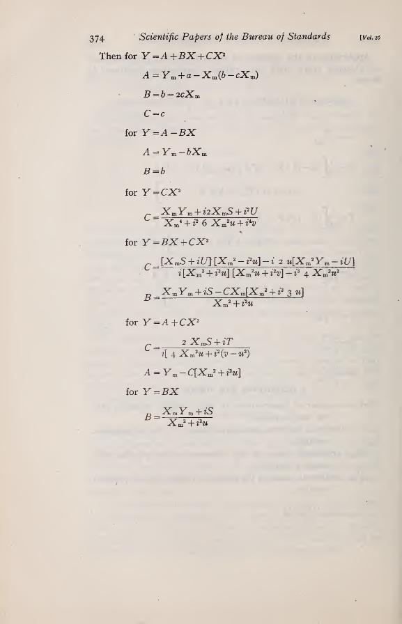
374 Scientific Papers of the Bureau of Standards [Voi.16
Then for Y =A +BX + CX*
A = Ym +a-Xm(b-cXm)
B = b-2cXm
C = c
for Y=A-BXA = Ym -bXm
B = b
for Y =CX2
XmYm + i2XmS + i2U
Xm* + i2 6 Xm
2u + i*v
for Y =BX +CX 2
[XmS + iU] [Xm2 - i2u] - i 2 u[Xm2Ym - iU]
C
B =
i[Xm2 + i2u] [Xm2u + i
2v] - i* 4 Xm
2u>
XmYm + iS-CXm[Xm2 + i23 u]
Xm2 + i2u
for Y=A+CX2
C = -2 XmS + iT
i[ + Xm2u + i2(v-u2
)
A = Ym -C[Xm2 + i2u]
for Y=BXXmYm + iSB = Xm2 + i
2u

Roeser) Adjustment of Curves to Observations, Etc. 375
TABLE 5.—Values of Coefficients for Use in the Least Squares Solution of Parabolic
and Linear Equations
log u, 1log¥ W
9. 6989700-10 0. 71429
9. 5351132 .46875
9. 3979400 . 33333
9. 2798407 . 25000
9. 1760913 . 19481
9. 0835461 . 15625
9. 0000000 . 12821
8. 9238452 . 10714
8. 8538720 .090909
8. 7891466 . 078125
8. 7289333 . 067873
8. 6726410 . 059524
8. 6197888 . 052632
8. 5699787 . 046875
8. 5228787 . 042017
8. 4782084 .037879
8. 4357285 .034325
8. 3952341 .031250
8. 3565473 . 028571
8.3195134 . 026224
8. 2839967 . 024155
8. 2498775 . 022321
8. 2170499 . 020690
8. 1854195 .019231
8. 1549020 .017921
8. 1254215 . 016741
8. 0909700 . 015674
log wn anevennum-ber
(n-l)«wanevennum-ber
6. 8000
14. 736
28.000
48. 562
78. 667
120. 86
178.00
253. 26
350. 00
472. 06
623. 47
808. 56
1032.
1298. 8
1614.
1983. 4
2412. 7
2908.
1
3476.0
4123.
3
4856.
8
5684.1
6612.7
7650.
6
8806.
11504
2. 0000
2. 9167
4.0000
5.2500
6. 6667
8. 2500
10. 000
11.917
14.000
16. 250
18. 667
21. 250
24. 000
26. 917
30. 000
33. 250
36. 667
40. 250
44. 000
47.917
52. 000
56. 250
60. 667
65. 250
70. 000
74. 917
80. 000
0. 3010300
. 4648868
. 6020600
. 7201593
. 8239087
. 9164539
1. 0000000
1. 0761548
1. 1461280
1. 2108534
1. 2710667
1. 3273589
1. 3802112
1. 4300213
1. 4771213
1. 5217916
1. 5642715
1. 6047659
1. 6434527
1. 6804866
1. 7160033
1. 7501225
1. 7829501
1. 8145805
1. 8450980
1. 8745785
1. 9090300
0. 50000
. 34285
. 25000
.19048
. 15000
. 12121
. 10000
. 083916
. 071429
. 061538
. 053571
. 047059
. 041667
. 037152
. 033333
. 030075
. 027273
. 024845
. 022727
. 020870
. 019231
. 017778
. 016484
. 015326
. 014286
.013348
. 012500
8538720-10
6709413
5228787
3979400
2896006
1938200
1079054
0299633
9586074
8927900
8316990
7746908
7212464
6709413
6234231
5783961
5356099
4948500
4559320
4186953
3829997
3487220
3057533
2839967
2533658
2237833
1951798
16
25
36
49
64
81
100
121
144
169
196
225
256
289,
324
361
400
441
484
529
576
625
676
729
784
841
900
Washington, February 20, 1920.


Top Related