


Languages
Pages
Legal

Which Factors Drive Rental Depreciation Rates for Office and Industrial Properties?
NEIL CROSBY, Real Estate & Planning, Henley Business School, University of Reading, Reading, RG6
6UD, UK, [email protected]
STEVEN DEVANEY, Real Estate & Planning, Henley Business School, University of Reading, Reading, RG6
6UD, UK, [email protected]
ANUPAM NANDA, Real Estate & Planning, Henley Business School, University of Reading, Reading, RG6
6UD, UK, [email protected]
ABSTRACT
As new buildings are constructed in response to changes in technology or user requirements, the
value of the existing stock will decline in relative terms. This is termed economic depreciation
and it may be influenced by the age and quality of buildings, amount and timing of expenditure,
and wider market and economic conditions. This study tests why individual assets experience
different depreciation rates, applying panel regression techniques to 375 UK office and industrial
assets. Results suggest that rental value depreciation rates reduce as buildings get older, while a
composite measure of age and quality provides more explanation of depreciation than age alone.
Furthermore, economic and local real estate market conditions are significant in explaining how
depreciation rates change over time.
ACKNOWLEDGMENTS
This research was funded and commissioned through the Investment Property Forum Research
Programme 2011–2015. The research team wishes to thank IPD and CBRE, in particular, for the
provision of data and the Investment Property Forum project steering group for their advice and
comments. We also thank the editor and reviewers for comments that have improved the paper.
1
Which Factors Drive Rental Depreciation Rates for Office and Industrial Properties?
ABSTRACT
As new buildings are constructed in response to changes in technology or user requirements, the
value of the existing stock will decline in relative terms. This is termed economic depreciation
and it may be influenced by the age and quality of buildings, amount and timing of expenditure,
and wider market and economic conditions. This study tests why individual assets experience
different depreciation rates, applying panel regression techniques to 375 UK office and industrial
assets. Results suggest that rental value depreciation rates reduce as buildings get older, while a
composite measure of age and quality provides more explanation of depreciation than age alone.
Furthermore, economic and local real estate market conditions are significant in explaining how
depreciation rates change over time.
1. INTRODUCTION
Depreciation affects all office and industrial buildings and it impacts on both real estate investors
and occupiers. As buildings deteriorate, or as technologies and user requirements change, they
become less suitable for their original use and require expenditure to mitigate any consequent
loss of productivity and value. A reduction in suitability may translate into longer vacancies and
reduced rental bids from potential occupiers. Thus, investors will be concerned to ensure that
any buildings in their portfolio remain competitive so that income is maintained and vacancy is
reduced. Failure to address depreciation can impact on investment returns as can failure to make
appropriate allowance for it when pricing and acquiring real estate assets.
In this context, judgements about the impact of depreciation on buildings and how this may vary
across regions, generations of buildings or property types, are important as they influence inputs
to pricing models such as rates of rental growth and assumptions about future expenditure. The
future may not behave like the past, but research into past causes of depreciation should improve
2
knowledge about how cash flows and values might change through time given different market
conditions and building characteristics. This can facilitate better decision making, such as on the
optimum time and level of refurbishment, or on when to redevelop in cases where depreciation
has been substantial and expenditure on the existing asset is no longer economically viable.
Depreciation in either the rental or capital values of commercial real estate has been measured by
several studies, reviewed below, and its causes have been debated. These causes include aging,
market state, asset quality and how buildings are leased and managed. However, there is a lack of
research that directly links depreciation rates experienced by commercial buildings to potential
drivers of those rates. It is this gap in existing research that this paper addresses, focusing on
depreciation in market rental values. Market rental values refer to the annual rent that could be
achieved on a new lease at a given point in time and these translate into cash flow adjustments at
market-based rent reviews or on reletting.
Regression models are estimated to identify the main drivers of annual rental value depreciation
rates over the period 1994 to 2009. These are applied to a panel dataset covering 375 office and
industrial buildings in the United Kingdom. The results suggest that depreciation rates reduce as
buildings get older, while a measure capturing both age and quality provides more explanation of
differences between assets than age alone. Furthermore, the state of the economy and local real
estate market are significant in explaining how depreciation rates change over time. The paper
proceeds by reviewing causes of depreciation first before discussing the empirical framework and
dataset that is used. The results are then set out in detail before a final section concludes.
2. REVIEW OF EXISTING LITERATURE
Exploration of economic depreciation began with Hotelling (1925) and was extended by Hulten
& Wykoff (1976; 1981; 1996) and others, resulting in its measurement for a wide range of assets.
In the real estate literature, depreciation has been studied for retail (Colwell & Ramsland, 2003),
3

apartments (Fisher et al., 2005) and hotels (Corgel, 2007) as well as for UK office and industrial
properties (see Salway, 1986; Baum, 1991; Baum, 1997; Barras & Clark, 1996; CEM, 1999; Dunse
& Jones, 2005). Two strands in the real estate literature on depreciation relate to its measurement
and causes. The measurement debate is set out in Dixon et al. (1999) and Crosby et al. (2012), so
this review concentrates on causes. Nonetheless, this study analyses depreciation rates that result
from a particular definition and measurement method, one that is consistent with seminal work
in this area (e.g. Hulten & Wykoff, 1981) and which has been refined for measuring depreciation
rates for real estate investments within a longitudinal framework. The definition for depreciation
is as follows:
“the rate of decline in rental/capital value of an asset (or group of assets) over time
relative to the asset (or group of assets) valued as new with contemporary specification”
Law (2004: 242)
To operationalize this definition for a longitudinal dataset, Hoesli & MacGregor (2000: 154) and
Law (2004) then propose the following formula to measure depreciation rates:
t1b
t2b
t1a
t2a
R/RR/R1d −= (1)
Where d = the rate of depreciation, Ra = asset rental value, Rb = benchmark rental value, t1 =
start of period and t2 = end of period.
This formula measures depreciation as a relative concept, comparing the value of an individual
asset through time against that of a benchmark for new properties in the same location. It is
common in the real estate literature to measure depreciation in relative terms, even if the exact
approach or formulas adopted have varied. However, this differs from an accounting perspective
4

where depreciation is a consumption concept where allowances are made for absolute reductions
in value, though such reductions are meant to proxy underlying economic processes (on which,
see Ben-Shahar et al., 2009). In a relative framework, having a benchmark for the same location
is important if the measurement of depreciation is to isolate asset-related changes in value from
wider market trends.
Causes of depreciation to rental and capital values of commercial real estate assets are commonly
divided into physical deterioration and various forms of obsolescence. Physical deterioration is a
function of the passage of time or aging and can be linked to the life cycle of buildings. In
contrast, obsolescence is hard to predict and makes the impact of age harder to predict, as
differently aged buildings reflect different designs, materials and specifications. In addition, there
will be variations in quality between properties of the same age that could be as important in
determining susceptibility to deterioration and obsolescence as age itself (Baum, 1993). The
unpredictable nature and timing of obsolescence suggests that the shape of depreciation will be
difficult to predict.
Nonetheless, there are some commonly hypothesised patterns in respect to age that either capital
or rental values might follow (see Hulten & Wykoff, 1981; Dixon et al., 1999). These are linear
depreciation, geometric depreciation (linear % change), S-curve and one-hoss shay, the latter
being an extreme case where values do not fall away in relative terms until some event leads to
an entire loss of value. These shapes are illustrated in Exhibit 1 for a hypothetical property of a
given life (value on the y-axis relates to the building element of value alone). Depending on their
quality or design, individual assets will vary both in terms of their useful economic life and the
pattern of depreciation that they will experience. Notwithstanding this, research has attempted to
discern whether typical patterns exist for different types of properties.
[INSERT EXHIBIT 1 HERE]
5

Hulten & Wykoff (1981) support a geometric pattern in depreciation for commercial and
industrial buildings in the US. They actually found a shape that was steeper than geometric, but
suggested that a geometric profile was a good approximation.1 Colwell & Ramsland (2003) found
that depreciation in prices of US department stores was high in the first 16 years and virtually
zero after this point, but Corgel (2007) found an “S” curve pattern for hotel sale prices and that
the critical age for slower depreciation was later at 28 years. Meanwhile, Dermisi & McDonald
(2010) found that sale prices for office buildings declined more steeply with age in the early years
of a building’s life, after controlling for quality and renovation activity. However, older cohorts
represent buildings that have survived pressures to redevelop during those periods, so survivor
bias may influence the results.
For UK commercial real estate, Salway (1986) suggested a geometric or steeper pattern of decline
in both rental and capital values, with high depreciation rates for the early years of a building’s
life. In contrast, analysis by Barras & Clark (1996) and Baum (1997) for office buildings in the
City of London suggests an S-curve for rental and capital values, with depreciation rates lower
for the first few years, then higher for several years before falling again after buildings were c. 15
years old. Results in CEM (1999) point to a similar pattern in office rental values, but the slowing
in depreciation appears to begin later. These studies are undertaken at different time points and
using different samples and measurement methods, so there is no firm consensus on the shape
of depreciation.
Owners can react to physical deterioration and obsolescence by undertaking capital expenditure
and the ultimate cure is redevelopment where depreciation in an existing asset is incurable or the
costs are too high to warrant a cure (see Colwell, 1991).2 Colwell & Ramsland (2003) and Corgel
(2007) discuss the role of expenditure and the lack of depreciation in older stock in the context
of reaching an optimum refurbishment date. Crosby et al. (2012) find that capital expenditure is
6
associated with lower rental value depreciation rates for UK commercial real estate. Hence,
depreciation can be influenced by the approach taken to the management of a building. Blazenko
& Pavlov (2004) explore the circumstances under which managers undertake expenditure, with
location and quality of an asset affecting likely pay-offs from such activities. Furthermore, lease
structures dictate who is responsible for repairs and can restrict the actions of different parties to
the lease.3
The role of land values must be also considered. Depreciation rates are typically measured using
prices or appraised values that relate to the total value or rent and do not distinguish between
building and land elements. Yet while the building element of value is likely to decline over time,
driven by deterioration and obsolescence, the land element may rise or fall with the demand for
and supply of sites in that location. As such, land value may protect total investment value to a
greater extent in locations where land is a large proportion of that total value. However, whether
a higher land value relative to total value protects rents is less clear. It is possible that, in different
locations, tenants pay similar relative rents for similar accommodation, which suggests that the
relative share of land value has little impact on rental depreciation rates and that its influence is
reflected in absolute differences in rental values at any point in time.4
Dunse & Jones (2005) note that several studies of real estate depreciation attempt to control for
location, which implies that location was expected to have an impact. They discuss whether rates
of depreciation may be higher where building value is a greater proportion of total value and the
land content is relatively low. They identify that locational obsolescence leading to site value
depreciation can occur, but land values can equally increase while buildings are subject to the
“inevitable march to the scrapheap” (Bowie, 1984), even though that scrapheap may be many
years into the future. Yet their results are inconclusive on whether higher site values generate
lower rental depreciation rates in the case of industrial properties.
7
Meanwhile, how depreciation behaves over time and in relation to real estate market conditions
needs more research. Hulten & Wykoff (1996) note how the age-price profile of assets can shift
from year to year in response to economic conditions while Dunse & Jones (2005) discuss the
influence of market state in a real estate context. Crosby et al. (2011) show how depreciation
rates in European office markets rise and fall with the cycle. They found that rental depreciation
was higher in strong markets and lower in weak markets, when prime rental values fell further
than those for average quality assets. Smith (2004) finds that residential depreciation rates vary
from year to year, though he does not identify whether different market states influence the
outcome. To fully address these issues, data on real estate markets and the wider economy need
to be examined.
This review identifies several factors that may explain why rental depreciation rates vary between
buildings and over time. The next section examines the methods used in this study to analyse
such variations.
3. EMPIRICAL FRAMEWORK
Real estate depreciation studies have varied as to whether longitudinal or cross-sectional datasets
and methods are used. Both approaches exhibit strengths and weaknesses either on conceptual
grounds or in terms of practical implementation, as discussed by Dixon et al. (1999) and Crosby
et al. (2012). However, to control adequately for the effects of time period, age and cohorts of
buildings from different eras, panel data is required. This can be difficult to obtain for individual
real estate assets as they may not be rented or traded frequently. Yet owing to the fact that some
types of investors must produce regular asset revaluations, it is possible to study panels of
appraisal based estimates of capital value and, in certain countries, market rental value. Panel data
on market rental values for individual buildings are used here.
8
There are many benefits from using panel data and associated econometric techniques (Hsiao,
2003; Baltagi, 2008). These include the fact that there is more variability and less collinearity in
the data, and the ability of the techniques to address heterogeneity at the unit level, as well as
study the dynamics of adjustment. However, panel data has potential issues such as measurement
error, the relative length of time series information and selectivity problems, although such issues
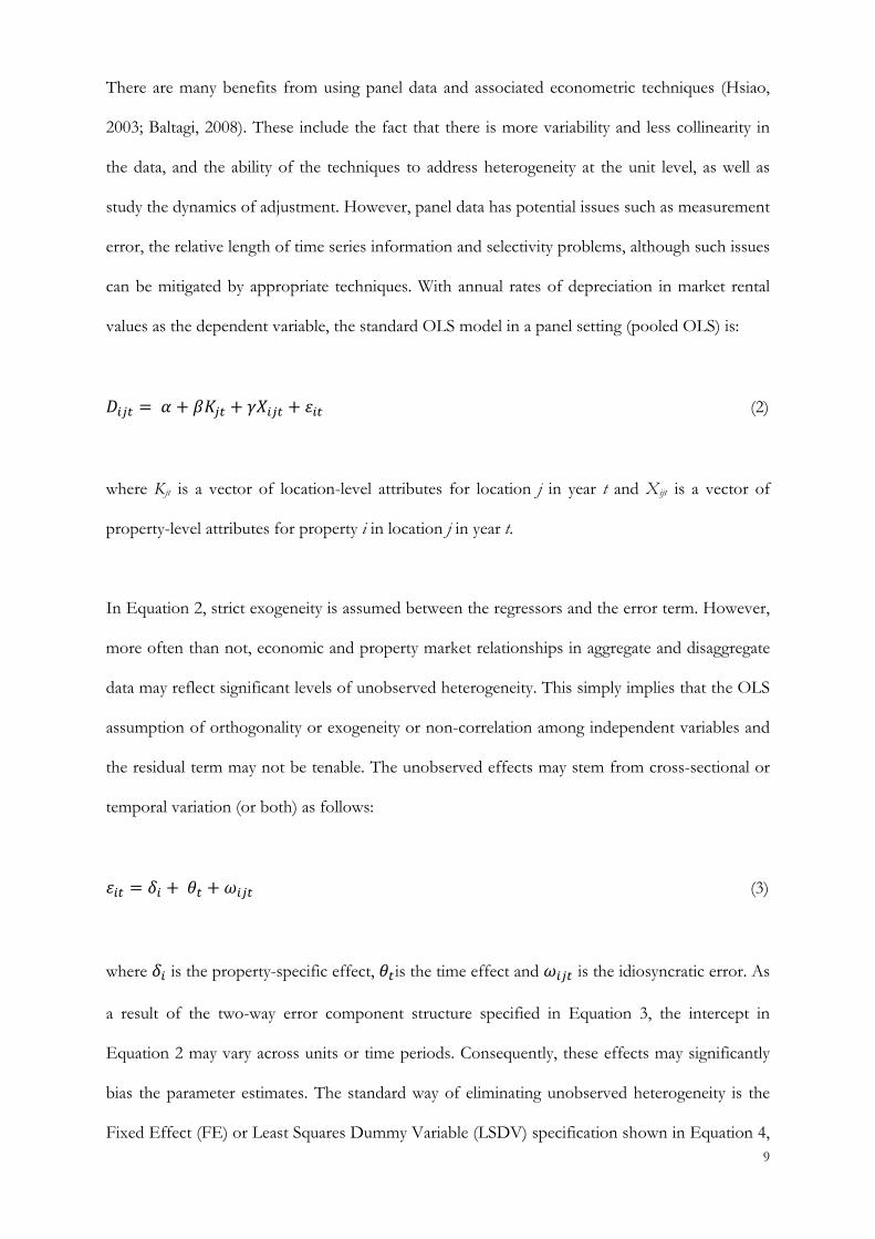
can be mitigated by appropriate techniques. With annual rates of depreciation in market rental
values as the dependent variable, the standard OLS model in a panel setting (pooled OLS) is:
𝐷𝐷𝑖𝑖𝑖𝑖𝑖𝑖 = 𝛼𝛼 + 𝛽𝛽𝐾𝐾𝑖𝑖𝑖𝑖 + 𝛾𝛾𝛾𝛾𝑖𝑖𝑖𝑖𝑖𝑖 + 𝜀𝜀𝑖𝑖𝑖𝑖 (2)
where Kjt is a vector of location-level attributes for location j in year t and Xijt is a vector of
property-level attributes for property i in location j in year t.
In Equation 2, strict exogeneity is assumed between the regressors and the error term. However,
more often than not, economic and property market relationships in aggregate and disaggregate
data may reflect significant levels of unobserved heterogeneity. This simply implies that the OLS
assumption of orthogonality or exogeneity or non-correlation among independent variables and
the residual term may not be tenable. The unobserved effects may stem from cross-sectional or
temporal variation (or both) as follows:
𝜀𝜀𝑖𝑖𝑖𝑖 = 𝛿𝛿𝑖𝑖 + 𝜃𝜃𝑖𝑖 + 𝜔𝜔𝑖𝑖𝑖𝑖𝑖𝑖 (3)
where 𝛿𝛿𝑖𝑖 is the property-specific effect, 𝜃𝜃𝑖𝑖is the time effect and 𝜔𝜔𝑖𝑖𝑖𝑖𝑖𝑖 is the idiosyncratic error. As
a result of the two-way error component structure specified in Equation 3, the intercept in
Equation 2 may vary across units or time periods. Consequently, these effects may significantly
bias the parameter estimates. The standard way of eliminating unobserved heterogeneity is the
Fixed Effect (FE) or Least Squares Dummy Variable (LSDV) specification shown in Equation 4, 9
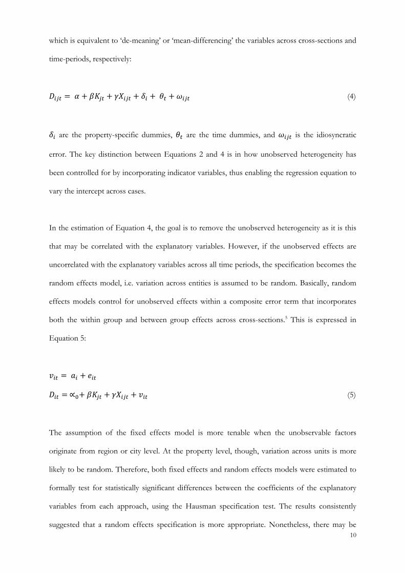
which is equivalent to ‘de-meaning’ or ‘mean-differencing’ the variables across cross-sections and
time-periods, respectively:
𝐷𝐷𝑖𝑖𝑖𝑖𝑖𝑖 = 𝛼𝛼 + 𝛽𝛽𝐾𝐾𝑖𝑖𝑖𝑖 + 𝛾𝛾𝛾𝛾𝑖𝑖𝑖𝑖𝑖𝑖 + 𝛿𝛿𝑖𝑖 + 𝜃𝜃𝑖𝑖 + 𝜔𝜔𝑖𝑖𝑖𝑖𝑖𝑖 (4)
𝛿𝛿𝑖𝑖 are the property-specific dummies, 𝜃𝜃𝑖𝑖 are the time dummies, and 𝜔𝜔𝑖𝑖𝑖𝑖𝑖𝑖 is the idiosyncratic
error. The key distinction between Equations 2 and 4 is in how unobserved heterogeneity has
been controlled for by incorporating indicator variables, thus enabling the regression equation to
vary the intercept across cases.
In the estimation of Equation 4, the goal is to remove the unobserved heterogeneity as it is this
that may be correlated with the explanatory variables. However, if the unobserved effects are
uncorrelated with the explanatory variables across all time periods, the specification becomes the
random effects model, i.e. variation across entities is assumed to be random. Basically, random
effects models control for unobserved effects within a composite error term that incorporates
both the within group and between group effects across cross-sections.5 This is expressed in
Equation 5:
𝑣𝑣𝑖𝑖𝑖𝑖 = 𝑎𝑎𝑖𝑖 + 𝑒𝑒𝑖𝑖𝑖𝑖
𝐷𝐷𝑖𝑖𝑖𝑖 = ∝0+ 𝛽𝛽𝐾𝐾𝑖𝑖𝑖𝑖 + 𝛾𝛾𝛾𝛾𝑖𝑖𝑖𝑖𝑖𝑖 + 𝑣𝑣𝑖𝑖𝑖𝑖 (5)
The assumption of the fixed effects model is more tenable when the unobservable factors
originate from region or city level. At the property level, though, variation across units is more
likely to be random. Therefore, both fixed effects and random effects models were estimated to
formally test for statistically significant differences between the coefficients of the explanatory
variables from each approach, using the Hausman specification test. The results consistently
suggested that a random effects specification is more appropriate. Nonetheless, there may be 10

unobserved time effects that call for being treated as fixed effects and so time fixed effects were
included in the random effects models to capture any broad temporal patterns in depreciation
rates, while other variables were used to explain the remaining variation, i.e. case-specific time
variation.
Although fixed effects and random effects models are natural candidates for use with panel data,
a potential issue is that the market rental values from which depreciation rates are measured are
appraisal based and so may be affected by appraisal smoothing.6 Quan & Quigley (1991) show
that, in the presence of noisy price signals, partial reliance on previous appraisals can be optimal
for an appraiser in terms of minimising overall error in individual appraisals. Yet it can lead to
movements in capital or rental values for individual assets being understated relative to the true,
but unobserved, movements. This would cast doubt on the validity of an analysis of periodic
changes.
However, research by Cheng et al. (2011) suggests that temporal changes in appraiser behaviour
and differences across appraisers mean that smoothing is not a guaranteed feature of appraisal
data. Furthermore, the effects of any appraisal smoothing on measurements of depreciation are
unclear. This is because depreciation rates are computed with reference to changes in both asset
values and benchmarks of new values, as shown by Equation 1. If the benchmarks are appraisal
based and exhibit similar levels of smoothing, then it is conceivable that the net effect on the rate
of depreciation might be neutral.7 Nonetheless, to address concerns that smoothing might distort
short term measurements of depreciation rates, the average annual rental value depreciation rate
for each asset is analysed in addition to the rates for each year. This is to see whether consistent
findings about factors influencing depreciation are reached.
To do this, a complementary procedure known as between effects regression is used with the
mean values of the variables (dependent and independent) for each case. This procedure explains
11

variation between cases in terms of their average experience across a period rather than utilising
variation over time in the variables. Together, random effects and between effects regressions
can be used to explore both the time-series and cross-sectional dimensions of a panel dataset.
Equation 6 is the Between Effects (BE) specification of the regression model, where the average
over time is modelled and so the cross-sectional variation is exploited.
𝐷𝐷�𝑖𝑖 = ∝0+ 𝛽𝛽𝐾𝐾�𝑖𝑖 + 𝛾𝛾𝛾𝛾�𝑖𝑖𝑖𝑖 + 𝑒𝑒𝑖𝑖 (6)
The long term average depreciation rate should be less susceptible to distortion from smoothing
provided that the period analysed spans a full cycle in the rental market.
4. DATA DESCRIPTION
Most of the data comes from two sources. First, IPD permitted access to anonymised data for
217 offices and 158 industrial and warehouse buildings spread throughout the UK.8 The data
include annual estimates of the market rental value for each building from the end of 1993 to the
end of 2009, as well as figures for capital expenditure and characteristics such as city, date of
construction and floorspace. The study period spans two complete cycles in UK office rents with
national IPD indices showing peaks in 2001 and 2007, and troughs in 1995, 2004 and 2009. It
also spans most of a longer cycle in UK industrial rents, with a peak in 2007 and troughs in 1995
and 2011.
Second, CBRE provided annual estimates for a wide range of locations of the rent that could be
achieved on a new lease and the capitalization rate achievable on sale for a hypothetical new asset
of a standard size and the highest specification appropriate for the location in question.9 More
than 200 office locations and more than 100 industrial locations in the UK are considered in this
exercise (CB Richard Ellis, 2007). These estimates were used as benchmarks, with each building
paired to the benchmark for the city or district in which it is located (large cities such as London
12

having multiple benchmarks). This matching was done to ensure that depreciation rates reflected
the effects of building related decline, not the performance of different cities or districts.
The hypothetical nature of the buildings in the CBRE benchmarks enables them to represent the
value of a new asset as required by Equation 1 in each and every period. It could introduce more
subjectivity into their estimation than a measure based solely on transactions, though. Since the
benchmarks for rental value are at city or district level and not site specific, some micro-location
shifts in value may be reflected in the depreciation rates. This will introduce some unavoidable
noise into the measurements and estimations.
Rental values are estimated assuming normal lease terms and these changed in the UK during the
study period, especially in regard to lease length (ODPM, 2005; IPD, 2014). Reductions in lease
lengths affect the assumptions used for both sample and benchmark rental values, but if they fell
more quickly for assets that are aging, this could have an impact on the rental values of the
sample assets and, thus, the depreciation rates. Meanwhile, unlike in the US, where there are
variations between assets and owners in the use of gross or net leases, UK leases are almost all
on a triple net basis and this has seen little change over the period being examined. Hence, both
sample and benchmark rental values represent payments for space alone and do not include any
allowance for associated operating expenses such as utilities, insurance or maintenance.
Predominantly, estimates of rental value are on a headline rather than an effective basis. In other
words, they represent rents received after any concessions such as rent-free periods, stepped rent
payments or capital contributions, including contributions to tenant fit-out costs by the landlord.
Any variation in concessions through time or across locations will be captured in both sample
and benchmark rental values. There may be differences between the concessions that are granted
when letting new assets (represented by the benchmarks) compared to the older stock in the
sample, though, which are not picked up in the data used here.
13
With these limitations in mind, annual changes in asset rental values were compared with annual
changes in the appropriate benchmarks to create annual rental value depreciation rates for each
building using Equation 1. This is the dependent variable in our analysis.
The literature review guided the selection of independent variables for the modelling. First, real
estate market conditions for places where sample assets are located were measured using the
CBRE series; computing the excess rental growth for a location relative to the national rental
growth rate in that period. Although the performance of each location is controlled for in the
measurement of depreciation, the strength or weakness of the market may influence how actors
in that location perceive assets of different ages or quality and whether or not new space is
constructed. Thus, in between effects models, the excess growth variable distinguishes high
growth from low growth locations while, in random effects models, it also identifies fluctuations
in local market fortunes over time.
Second, the effect of aging is tested using an age variable based on the construction date of each
asset as recorded by IPD. This date field captures either the year when the asset was built or the
year of its last major refurbishment. Ideally, separate dates for these events would be recorded,
but only a composite field was available. Age is measured as at end-1993 and different functional
forms for the variable were tested including linear, log and squared forms as well as splines for
predefined age groups. The motive for splines was to test if depreciation rates varied in a non-
linear fashion for buildings from different eras or at different stages of their life. Splines could
enable an S-curve or other irregular pattern in depreciation to be detected, but a single spline
point performed better than a set of splines for these samples. Other functional forms assisted in
testing for geometric, concave or convex patterns in the age-depreciation relationship.
14
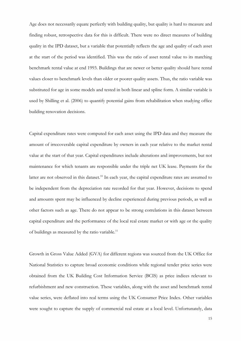
Age does not necessarily equate perfectly with building quality, but quality is hard to measure and
finding robust, retrospective data for this is difficult. There were no direct measures of building
quality in the IPD dataset, but a variable that potentially reflects the age and quality of each asset
at the start of the period was identified. This was the ratio of asset rental value to its matching
benchmark rental value at end 1993. Buildings that are newer or better quality should have rental
values closer to benchmark levels than older or poorer quality assets. Thus, the ratio variable was
substituted for age in some models and tested in both linear and spline form. A similar variable is
used by Shilling et al. (2006) to quantify potential gains from rehabilitation when studying office
building renovation decisions.
Capital expenditure rates were computed for each asset using the IPD data and they measure the
amount of irrecoverable capital expenditure by owners in each year relative to the market rental
value at the start of that year. Capital expenditures include alterations and improvements, but not
maintenance for which tenants are responsible under the triple net UK lease. Payments for the
latter are not observed in this dataset.10 In each year, the capital expenditure rates are assumed to
be independent from the depreciation rate recorded for that year. However, decisions to spend
and amounts spent may be influenced by decline experienced during previous periods, as well as
other factors such as age. There do not appear to be strong correlations in this dataset between
capital expenditure and the performance of the local real estate market or with age or the quality
of buildings as measured by the ratio variable.11
Growth in Gross Value Added (GVA) for different regions was sourced from the UK Office for
National Statistics to capture broad economic conditions while regional tender price series were
obtained from the UK Building Cost Information Service (BCIS) as price indices relevant to
refurbishment and new construction. These variables, along with the asset and benchmark rental
value series, were deflated into real terms using the UK Consumer Price Index. Other variables
were sought to capture the supply of commercial real estate at a local level. Unfortunately, data
15

on vacancy rates, starts or completions could not be obtained at sufficient disaggregation to be
useful in this study, though.
Meanwhile, in the absence of robust and publicly available data on land values, an exercise was
undertaken to generate office and industrial land value estimates for each location in the dataset.
This was done by creating a hypothetical capital value per square metre for a new building in
each location using rents and yields from CBRE and then subtracting an estimated development
cost per square metre. This is in line with the residual calculation of site value used in the UK
real estate industry (Coleman et al., 2013) although alternative methods for estimating land values
exist and have been recently reviewed by Ozdilek (2015). The calculation used here is expressed
by the following equation:
𝐿𝐿𝐿𝐿0 = (1 + 𝑖𝑖)−𝑖𝑖 � 𝐷𝐷𝐷𝐷0(1+𝑝𝑝)
− 𝐷𝐷𝐷𝐷0 − 𝐼𝐼� (7)
Where LV0 is residual land value at time t = 0, i equals an annual interest rate and t =
development period, while DV0 = current estimate of development value per square metre, p =
profit as a percentage of DV0, DC0 = current estimate of development costs per square metre
and I = finance costs.
Development costs (DC0) were based on current BCIS figures for construction cost per square
metre for office or industrial buildings in different areas, these being deflated with the nominal
tender price indices to produce a historical time series. A development period (t) of 2 years for
offices and 1.5 years for industrial buildings was adopted and professional fees based on 10% of
construction costs were added to those costs. Profit (p) was allowed for at a standard rate of 15%
of development value and finance rates (i) at each date were based on three month LIBOR plus a
margin for speculative development finance.12 Finance costs (I) were calculated by charging
interest on construction costs and fees over half the development period to reflect that not all 16

such costs are incurred immediately. The resulting residual value per square metre was then
discounted over the development period at the finance rate.
Given the number of assumptions and inputs needed to estimate land values, it is likely they do
not measure the level of land value particularly accurately. This would be a major limitation if we
sought to partition the rental figures into land related and building related elements (for which
see Smith (2004) for a successful example in relation to house prices). Therefore, they are used
solely as an independent variable to control for the impact of relative differences in land values
across locations.13 The variable used in the models that follow is the proportion of land value to
total development value (i.e. LV0/DV0). It is possible for this variable to take a negative value in
some locations or periods where development costs were estimated to be greater than the values
of completed buildings.
5. PANEL MODELLING AND RESULTS
Annual rates of rental value depreciation have been analysed using random effects models. These
explore drivers of changes in depreciation rates over time. However, as the annual rates may be
susceptible to distortion from appraisal smoothing, long term average depreciation rates are also
studied using between effects models. To test the robustness of the findings further, the analysis
considers both the entire sixteen years spanned by the dataset, 1994-2009, and a nine year sub-
period from 1997-2005. This is because the start and end years for the longer period fall within
major UK real estate downturns that may have increased difficulties for appraisers in judging
market rental values owing to a reduced volume of rental transactions. In contrast, 1997-2005
represents a period of relative stability.
Modelling is conducted using 206 office and 143 industrial buildings. The sectors are modelled
separately because although qualitatively similar patterns emerge from each sample, a pooled
model produces results that mask sector heterogeneity. Reductions in sample size from the
17

original samples reflect cases with missing data on one or more independent variables. Some
assets had extreme values in some years for certain variables: rental value depreciation rate,
benchmark excess growth rate, age, rental value ratio, floorspace and capital expenditure rate.
Rather than discard more data by removing the cases concerned, a winsorizing procedure was
used whereby extreme values were replaced with the values at a pre-defined percentile of the
distribution.14
Descriptive statistics relevant to the two modelling approaches are shown in Exhibit 2. Panel A
reports statistics in relation to the group means required for the between effects estimation and
Panel B reports statistics for the whole panel as utilised by the random effects technique. In the
latter case, sample size is determined both by the number of assets (n) and time periods (t) that
the dataset covers. The table clearly indicates the presence of extreme values and the benefits of
winsorizing the data. For example, the average rate of rental value depreciation is only 0% in the
original data with the mean skewed by some extreme cases of appreciation (where asset rental
values in some periods grew more quickly than their benchmark values). Nonetheless, models
were estimated using original values for all variables as well and the results from these are
qualitatively similar to those that are reported below.
[INSERT EXHIBIT 2 HERE]
Results are presented first for random effects models and then for between effects models.
Different functional forms are tested for some variables and lags are used in some models to
capture delays in the effects of certain variables on rental value depreciation rates. Robust
standard errors are used throughout to test the significance of coefficients.
18

5.1 Random effects models
Results for offices are shown in Exhibit 3 and results for industrial assets are shown in Exhibit 4.
In each case, six models are presented, representing three different specifications each of which
is tested over two periods: the full period and the nine-year sub-period.
Starting with offices, Exhibit 3 shows that changes in excess benchmark growth are positively
related to changes in rental value depreciation rates. This suggests that rates of depreciation for
existing buildings increase if rental growth in a location is relatively strong. In contrast, lagged
growth in real GVA has significant negative coefficients, which suggests that stronger economic
growth helps reduce rental value depreciation whereas strong real estate market growth does not
(the lag in the former indicating that it takes time for economic growth to translate into real
estate demand). Lagged changes in tender prices have significant negative coefficients. If a rise in
tender prices reduces production of new office space and, thus, competition from new buildings,
it makes sense that rental value depreciation rates would fall.
[INSERT EXHIBIT 3 HERE]
Negative coefficients for the linear age variable in the first two models point to reducing rates of
rental value depreciation as buildings age through time. In the third and fourth models, splines
for age are used and these divide the sample into two groups: offices between 0 and 40 years old
and those greater than 40 years old as at end-1993. This division was chosen after examining the
distribution of ages in the sample and because the early 1950s marked an upturn in UK office
building after a long period without development. This gap resulted from wartime and postwar
restrictions on both building materials and capital flows, while the design and construction of
offices around this time also changed (Barras, 2009). The coefficients suggest that depreciation
rates reduce with age in the 0-40 group, but not for buildings older than this. Testing of further
splines did not reveal any alternative patterns such as an S-curve in rental value depreciation.
19
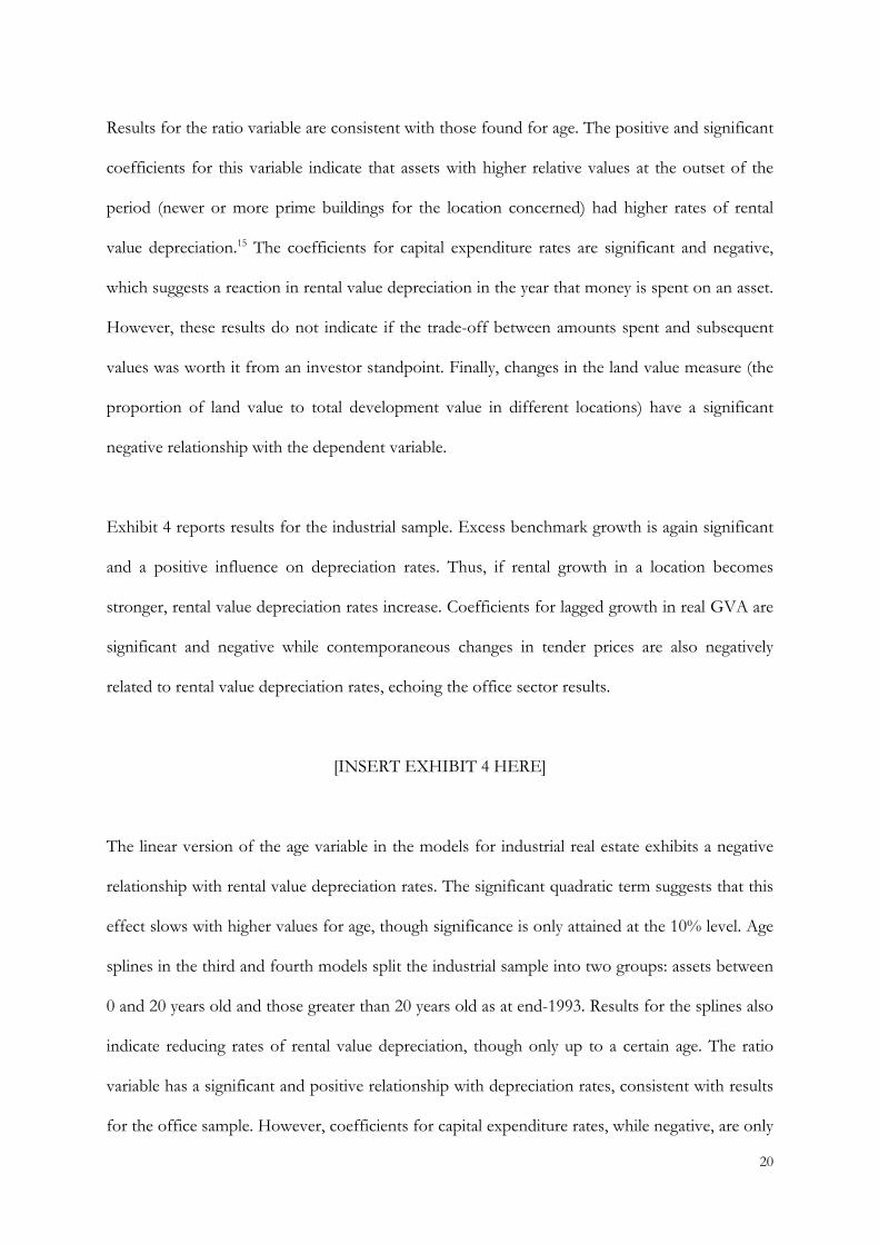
Results for the ratio variable are consistent with those found for age. The positive and significant
coefficients for this variable indicate that assets with higher relative values at the outset of the
period (newer or more prime buildings for the location concerned) had higher rates of rental
value depreciation.15 The coefficients for capital expenditure rates are significant and negative,
which suggests a reaction in rental value depreciation in the year that money is spent on an asset.
However, these results do not indicate if the trade-off between amounts spent and subsequent
values was worth it from an investor standpoint. Finally, changes in the land value measure (the
proportion of land value to total development value in different locations) have a significant
negative relationship with the dependent variable.
Exhibit 4 reports results for the industrial sample. Excess benchmark growth is again significant
and a positive influence on depreciation rates. Thus, if rental growth in a location becomes
stronger, rental value depreciation rates increase. Coefficients for lagged growth in real GVA are
significant and negative while contemporaneous changes in tender prices are also negatively
related to rental value depreciation rates, echoing the office sector results.
[INSERT EXHIBIT 4 HERE]
The linear version of the age variable in the models for industrial real estate exhibits a negative
relationship with rental value depreciation rates. The significant quadratic term suggests that this
effect slows with higher values for age, though significance is only attained at the 10% level. Age
splines in the third and fourth models split the industrial sample into two groups: assets between
0 and 20 years old and those greater than 20 years old as at end-1993. Results for the splines also
indicate reducing rates of rental value depreciation, though only up to a certain age. The ratio
variable has a significant and positive relationship with depreciation rates, consistent with results
for the office sample. However, coefficients for capital expenditure rates, while negative, are only
20
significant in the full period models while those for the land value variable are either insignificant
or positive.
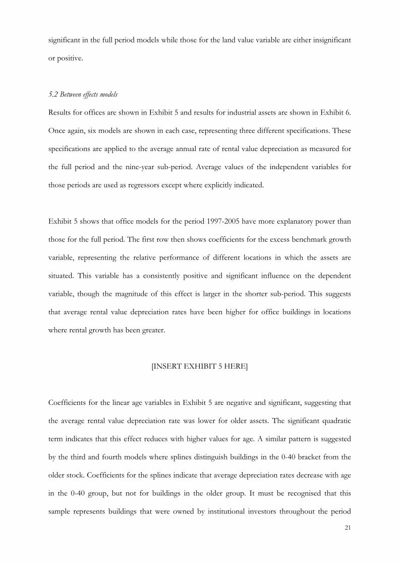
5.2 Between effects models
Results for offices are shown in Exhibit 5 and results for industrial assets are shown in Exhibit 6.
Once again, six models are shown in each case, representing three different specifications. These
specifications are applied to the average annual rate of rental value depreciation as measured for
the full period and the nine-year sub-period. Average values of the independent variables for
those periods are used as regressors except where explicitly indicated.
Exhibit 5 shows that office models for the period 1997-2005 have more explanatory power than
those for the full period. The first row then shows coefficients for the excess benchmark growth
variable, representing the relative performance of different locations in which the assets are
situated. This variable has a consistently positive and significant influence on the dependent
variable, though the magnitude of this effect is larger in the shorter sub-period. This suggests
that average rental value depreciation rates have been higher for office buildings in locations
where rental growth has been greater.
[INSERT EXHIBIT 5 HERE]
Coefficients for the linear age variables in Exhibit 5 are negative and significant, suggesting that
the average rental value depreciation rate was lower for older assets. The significant quadratic
term indicates that this effect reduces with higher values for age. A similar pattern is suggested
by the third and fourth models where splines distinguish buildings in the 0-40 bracket from the
older stock. Coefficients for the splines indicate that average depreciation rates decrease with age
in the 0-40 group, but not for buildings in the older group. It must be recognised that this
sample represents buildings that were owned by institutional investors throughout the period
21
concerned and some older buildings that were traded may have depreciated more rapidly.
Nonetheless, the results are consistent with vintage effects found in other studies (e.g. Colwell &
Ramsland, 2003; Corgel, 2007).
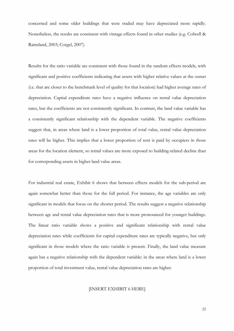
Results for the ratio variable are consistent with those found in the random effects models, with
significant and positive coefficients indicating that assets with higher relative values at the outset
(i.e. that are closer to the benchmark level of quality for that location) had higher average rates of
depreciation. Capital expenditure rates have a negative influence on rental value depreciation
rates, but the coefficients are not consistently significant. In contrast, the land value variable has
a consistently significant relationship with the dependent variable. The negative coefficients
suggest that, in areas where land is a lower proportion of total value, rental value depreciation
rates will be higher. This implies that a lower proportion of rent is paid by occupiers in those
areas for the location element, so rental values are more exposed to building-related decline than
for corresponding assets in higher land value areas.
For industrial real estate, Exhibit 6 shows that between effects models for the sub-period are
again somewhat better than those for the full period. For instance, the age variables are only
significant in models that focus on the shorter period. The results suggest a negative relationship
between age and rental value depreciation rates that is more pronounced for younger buildings.
The linear ratio variable shows a positive and significant relationship with rental value
depreciation rates while coefficients for capital expenditure rates are typically negative, but only
significant in those models where the ratio variable is present. Finally, the land value measure
again has a negative relationship with the dependent variable: in the areas where land is a lower
proportion of total investment value, rental value depreciation rates are higher.
[INSERT EXHIBIT 6 HERE]
22

5.3 Further robustness checks for office sample
Some issues that may distort the results are now investigated further. Three issues are analysed,
two of which relate specifically to the office data and the third of which is illustrated using the
office sample. For brevity, results are reported only for tests on the shorter sub-period, 1997-
2005.
First, the office sample has a large cluster of buildings in just one location: Central London. Out
of 206 office buildings available for modelling, 103 are in this area. The distinct nature of Central
London within the UK office market, both from an investor and occupier perspective, raises the
question of whether these assets may behave differently. To test this, models were re-estimated
using the subset of buildings in this area and then the remaining sample of buildings. Selected
coefficients from these models are shown in Exhibit 7.
[INSERT EXHIBIT 7 HERE]
Results for excess benchmark growth in Exhibit 7 echo those shown above for the sample as a
whole and the capital expenditure rate remains a significant variable in most models. Results for
age are weaker, though. The negative relationship between age and rental value depreciation rates
is still evident, but coefficients for these smaller samples are only significant in one instance. In
contrast, the ratio variable remains significant for both Central London assets (between effects)
and assets in the rest of the UK (between and random effects models). The land value measure is
no longer influential, but this may reflect that the biggest distinction in proportion of land value
to total value lies between Central London and the rest of the UK.
Second, there is a group of buildings in the office sample where reported age is greater than 50
years old. Although the age variable should recognise the timing of major refurbishments, it is
likely that some, if not all, of these cases will have been refurbished and modernised. Thus, the
23

recorded age may be a poor reflection of the effective age of the space. Therefore, models were
re-estimated using only those buildings whose recorded age at end 1993 was below 50 years. The
coefficients for selected models are shown in Exhibit 8 and suggest that the key result in relation
to the negative relationship between age and rental value depreciation rates remains.
[INSERT EXHIBIT 8 HERE]
Finally, a further test was made to see whether the inclusion of the land value measure distorts
the results. This variable could be challenged on the grounds of the number of assumptions and
inputs required for its construction. Coefficients for selected models that exclude this variable
are also shown in Exhibit 8. Once again, the results for other variables are fairly consistent with
those already presented and discussed.
6. SUMMARY
Depreciation in real estate values over time is an important issue in the pricing and management
of real estate investments. Large scale investors in commercial real estate model real estate assets
through time to identify the behaviour of different types of property, of different quality, within
prime and secondary markets. More detailed datasets are now emerging that enable the life cycle
of buildings to be analysed for the purpose of modelling cash flows and determining in advance
optimum refurbishment and redevelopment periods. Depreciation rates play an important part in
this process and the findings in this paper should enable such rates to be applied within a more
fine-grained process; concerning, for example, shape of depreciation, newer against older assets,
impact of periodic expenditure and impact of different market states. Owing to data limitations,
much prior research concentrated on measuring depreciation rather than testing the causes. This
paper seeks to begin to address this imbalance.
24

Specifically, this paper empirically identifies causes of rental value depreciation rates for samples
of office and industrial buildings in the UK. The rate at which commercial real estate rents fall
through time relative to rents for new buildings influences the values of existing stock and is a
major driver of the timing of refurbishment or redevelopment. A dataset of rental value
depreciation rates for 375 UK office and industrial buildings was assembled as well as variables
that represent the potential major drivers of rental depreciation. These variables included the age
and quality of the buildings, the amount spent on them and estimates of land values. Panel data
techniques were then employed and robustness checks performed to reach consistent findings.
A major finding is that the higher quality properties in each market suffer more from rental value
depreciation than their lower quality counterparts. Quality is not measured directly, but has been
assessed for each building using the ratio of its rental value to an estimated benchmark value for
its location as at the start of the period. Results for age complement this finding as they suggest
that newer assets have higher rental value depreciation rates than older stock, though this effect
disappears after a certain age. In fact, if a property survives to a certain age, its rental value may
cease to deteriorate relative to new properties in that location. The analysis did not detect other
patterns in the earlier life or quality cycle of buildings such as an S-curve. The results appear to
be more consistent with a geometric or a steeper convex-to-origin profile in rental value
depreciation, echoing the findings of seminal research by Hulten & Wykoff (1981).
Another finding is that capital expenditure mitigates the effects of rental value depreciation. This
has been suggested before in previous research, but is confirmed here by analysis that controls
for other relevant drivers of depreciation rates. Meanwhile, the influence of land values on rental
value depreciation rates was tested by estimating office and industrial land values for different
locations. Where land value makes up a higher proportion of total value, this seems to reduce
rental value depreciation rates, suggesting that important differences in such rates will exist
25

across regions and within urban areas. However, improvements in land value data for the UK are
needed in order to confirm these findings.
How depreciation behaves through time has been the subject of inconclusive analysis in the past.
The time dummies in the random effects models did not show any consistent trend or cyclical
pattern in depreciation over this period and so were not reported. Yet there were clear findings
in relation to time variations specific to individual properties. Rental value depreciation rates are
increased in locations where growth is stronger than average and also holds over the longer term
as shown by the between effects results. However, when regional economic growth is strong,
both office and industrial depreciation rates appear to be reduced. It is difficult to reconcile these
findings, but they may reflect the interaction of economic and real estate cycles. When user
demand for a location is high, depreciation may be low at first as all buildings benefit. As
developers then respond to any upturn, competition for new space may drive stronger growth in
prime rents than in rents for existing assets, up until demand in the location is exhausted. After
this, prime rents may come under more pressure to fall, closing the gap between newer buildings
and the rest of the stock.
However, appraisal issues affecting rental values might be influencing the results, particularly if
there are differences in approach to appraising existing assets versus prime benchmarks. Thus,
future studies would benefit from creation of transaction based indexes of market rent to test the
findings further. Nonetheless, the approach taken here has yielded important insights into why
rental depreciation varies between buildings, both from period-to-period and in the longer term.
The results also suggest interesting areas for future research. Interactions between depreciation,
market conditions and the real estate development cycle is one such area, while the relationship
between rental depreciation, expenditure and lease terms also merits further attention.
26

ENDNOTES
1 Steeper refers to a higher rate of depreciation for the earlier years of an asset’s life than for later
years.
2 Renovation decisions are explored theoretically by Wong & Norman (1994) and, more recently,
Shilling et al. (2006).
3 Baum & Turner (2004) argued that long triple net leases in the UK, where responsibility for all
repairs was passed to tenants, encouraged owners to passively manage assets, with the effects of
depreciation only addressed at lease expiry. Such an approach may lead to greater depreciation in
the long run.
4 For example, if a new property in a high value location has a rental value of £100 and the same
property has a rental value of £50 in a lower value location, two identical 20 year old properties
in those locations might have rental values of £80 and £40, respectively, both representing
depreciation of 20% from new.
5 Note that the specification in Equation 5 implies that there may be substantial serial correlation
in the composite error term, which can be addressed by generalized least squares techniques.
6 See Edelstein & Quan (2006) for further discussion. Note that nearly all literature on appraisal
smoothing considers capital values rather than appraiser estimates of market rent.
7 Say that the true changes in asset and benchmark values are 3% and 6%, respectively, but the
appraisals show changes of 2% and 5% owing to smoothing. Using Equation 1, the true rate of
depreciation would be 2.83% while the measured rate would be 2.86%. This similarity in
outcomes will hold if the degree of smoothing in asset and benchmark rental values is similar.
8 IPD are part of MSCI and conduct real estate performance benchmarking for investors such as
insurance companies, pension funds and REITs. Information on assets in their database is not
normally available and was accessed under strict confidentiality arrangements.
27

9 CBRE are a global property services company. The data they provided underlies their UK Rent
and Yield Monitor publication.
10 Lack of maintenance during a lease should not significantly affect rental values as tenants are
legally required to address this under the UK triple net lease structure. In practice, there might be
incentive issues in terms of the degree of maintenance that tenants perform relative to owners –
see Wiley et al. (2014).
11 Correlations between average capital expenditure rates and benchmark rental growth rates are -
0.03 and -0.11 for office and industrial assets, respectively. Correlations between expenditure
rates and age are -0.07 and 0.01 for the office and industrial samples while they are 0.19 and 0.13
between expenditure rates and the ratios of asset to benchmark rental value.
12 The three month LIBOR rate was obtained from the Bank of England website. The margin
used by banks when lending against speculative development schemes is reported by Maxted and
Porter (various) in their annual survey of real estate lending activity. This survey only dates back
to 1999, so earlier figures for the margin were set at the 1999 rate.
13 Note that we measure the importance of land within a location generally and do not attempt to
estimate the specific value of each site and its contribution to the total value of each asset in the
sample, for which far more detailed comparable data would be required – see Ozdilek (2015) or
Shi (2015).
14 The threshold selected for the process was 2.5%, which meant truncating 1.25% of
observations in each tail of the distribution for these variables. One-tailed truncation was applied
in the case of both the age and capital expenditure rate variables in order to prevent the removal
of low values that are valid and not outliers.
15 Splines for the ratio variable were tested, but there was no obvious pattern in the coefficients
and so these results are not reported.
28
REFERENCES
Baltagi, B. H., Econometric Analysis of Panel Data, fourth edition, Wiley, 2008.
Barras, R. and P. Clark, Obsolescence and Performance in the Central London Office Market,
Journal of Property Valuation and Investment, 1996, 14: 4, 63-78.
Barras, R., Building Cycles: Growth & Instability, Oxford: Wiley-Blackwell, 2009.
Baum, A., Property Investment Depreciation and Obsolescence, London: Routledge, 1991.
Baum, A. E., Quality, Depreciation, and Property Performance, Journal of Real Estate Research,
1993, 8: 4, 541-565.
Baum, A., Trophy or Tombstone? A Decade of Depreciation in the Central London Office Market. London:
Lambert Smith Hampton and HRES, 1997.
Baum, A. and N. Turner, Retention Rates, Reinvestment and Depreciation in European Office
Markets, Journal of Property Investment and Finance, 2004, 22: 3, 214-235.
Ben-Shahar, D., Y. Margalioth and E. Sulganik, The Straight-Line Depreciation is Wanted, Dead
or Alive, Journal of Real Estate Research, 2009, 31: 3, 351-370.
Blazenko, G. W. and A. D. Pavlov, The Economics of Maintenance for Real Estate Investments,
Real Estate Economics, 2004, 32: 1, 55-84.
Bowie, N., The Depreciation of Buildings, Journal of Property Valuation and Investment, 1984, 2: 1, 5-
13.
CEM, The Dynamics and Measurement of Commercial Property Depreciation in the UK, Reading: College
of Estate Management, 1999.
Cheng, P., Z. Lin and Y. Liu, Heterogeneous Information and Appraisal Smoothing, Journal of
Real Estate Research, 2011, 33: 4, 443-469.
Coleman, C., N. Crosby, P. McAllister and P. Wyatt, Development appraisal in practice: some
evidence from the planning system, Journal of Property Research, 2013, 30: 2, 144-165.
Colwell, P. F., Functional Obsolescence and an Extension of Hedonic Theory, Journal of Real
Estate Finance and Economics, 1991, 4: 1, 49-58.
29

Colwell, P. F. and M. O. Ramsland, Coping with Technological Change: The Case of Retail,
Journal of Real Estate Finance and Economics, 2003, 26: 1, 47–63.
Corgel, J. B., Technological Change as Reflected in Hotel Property Prices, Journal of Real Estate
Finance and Economics, 2007, 34: 2, 257-279.
Crosby, N., S. Devaney and V. Law, Benchmarking and valuation issues in measuring
depreciation for European Office Markets, Journal of European Real Estate Research, 2011, 4:
1, 7-28.
Crosby, N., S. Devaney and V. Law, Rental Depreciation and Capital Expenditure in the UK
Commercial Real Estate Market, 1993-2009, Journal of Property Research, 2012, 29: 3, 227-246.
Dermisi, S. V. and J. F. McDonald, Selling Prices / Sq. Ft. of Office Buildings in Downtown
Chicago – How Much Is It Worth to Be an Old But Class A Building? Journal of Real Estate
Research, 2010, 32: 1, 1-21.
Dixon, T. J., N. Crosby and V. K. Law, A critical review of methodologies for measuring rental
depreciation applied to UK commercial real estate, Journal of Property Research, 1999, 16: 2,
153-180.
Dunse, N. and C. Jones, Rental Depreciation, Obsolescence and Location: the Case of Industrial
Properties, Journal of Property Research, 2005, 22: 2-3, 205-223.
Edelstein, R. H. and D. Quan, How Does Appraisal Smoothing Bias Real Estate Returns
Measurement? Journal of Real Estate Finance and Economics, 2006, 32: 1, 41-60.
Fisher, J. D., B. C. Smith, J. J. Stern and R. B. Webb, Analysis of Economic Depreciation for
Multi-Family Property, Journal of Real Estate Research, 2005, 27: 4, 355-369.
Hoesli, M. and B. M. MacGregor, Property Investment: Principles and Practice of Portfolio Management,
Harlow: Longman, 2000.
Hotelling, H., A General Mathematical Theory of Depreciation, Journal of American Statistical
Association, 1925, 20: 151, 340-53.
Hsiao, C., Analysis of Panel Data, second edition, Cambridge University Press, 2003.
30

Hulten C. R. and F. C. Wykoff., The Economic Depreciation of Non-Residential Structures, Working
Paper in Economics No 16, Baltimore: Johns Hopkins University, 1976.
Hulten C. R. and F. C. Wykoff, The Estimation of Economic Depreciation Using Vintage Asset
Prices: An Application of the Box-Cox Power Transformation, Journal of Econometrics, 1981,
15: 3, 367-396.
Hulten C. R. and F. C. Wykoff., Issues in the measurement of economic depreciation:
Introductory remarks, Economic Enquiry, 1996, 34: 1, 10-23.
IPD, UK Lease Events Review - November 2014, London: Investment Property Databank, 2014.
Jorgenson, D. W., Empirical Studies of Depreciation, Economic Enquiry, 1996, 34: 1, 24-42.
Law, V., The Definition and Measurement of Rental Depreciation in Investment Property, PhD dissertation,
Reading: University of Reading, 2004.
Maxted, B. and T. Porter, The UK Commercial Property Lending Market, Leicester: De Montfort
University, Various.
ODPM, Monitoring the 2002 Code of Practice for Commercial Leases, London: HMSO, 2005.
Ozdilek, U., Property price separation between land and building components, Journal of Real
Estate Research, Forthcoming, 2015.
Quan, D. C. and J. M. Quigley, Price Formation and the Appraisal Function in Real Estate
Markets, Journal of Real Estate Finance and Economics, 1991, 4: 2, 127-146.
Salway, F., Depreciation of Commercial Property, Centre for Advanced Land Use Studies, Reading:
College of Estate Management, 1986.
Shi, S., The Improved Net Rate Analysis, Journal of Real Estate Research, Forthcoming, 2015.
Shilling, J. D., K. D. Vandell, R. Koesman and Z. Lin, How Tax Credits Have Affected the
Rehabilitation of the Boston Office Market, Journal of Real Estate Research, 2006, 28: 4, 321-
348.
Smith, B. C., Economic depreciation of residential real estate: Microlevel space and time analysis,
Real Estate Economics, 2004, 32: 1, 161–180.
31
Wiley, J. A., Y. Liu, D. Kim and T. Springer, The Commercial Office Market and the Markup for
Full Service Leases, Journal of Real Estate Research, 2014, 36: 3, 319-340.
Wong, K. C. and G. Norman, The Optimal Time of Renovating a Mall, Journal of Real Estate
Research, 1994, 9: 1, 33-47.
ACKNOWLEDGMENTS
INSERT AFTER REVIEW
32
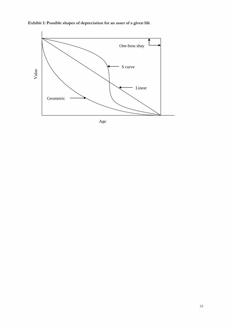
Exhibit 1: Possible shapes of depreciation for an asset of a given life
One-hoss shay
S curve
Linear
Geometric
Age
Val
ue
33

Exhibit 2: Means and standard deviations for office and industrial samples
Panel A: Descriptive statistics for group means
Offices (n = 206) Industrials (n = 143) Mean St Dev. Min Max Mean St Dev. Min Max Rental depreciation rate (%) 0.0 2.0 -7.1 5.2 0.1 1.6 -6.7 3.5 Winsorized 0.3 1.7 -5.1 5.2 0.1 1.4 -4.0 3.0 Excess benchmark growth (%) 1.2 2.2 -2.6 6.2 0.3 1.1 -1.4 2.2 Winsorized 1.1 2.2 -2.6 6.2 0.2 1.1 -1.4 2.6 Age at end-1993 35 50 1 263 13 7 1 45 Winsorized 35 47 1 193 13 7 1 45 Ratio at end-1993 71.3 33.6 3.3 260.5 84.7 30.0 11.9 219.6 Winsorized 70.4 30.6 5.2 126.9 84.0 27.6 16.3 132.1 Floorspace (sq. m.) 3,699 3,711 194 26,794 9,568 9,288 95 68,459 Winsorized 3,526 2,980 326 13,009 9,308 7,943 1,525 40,629 Capital expenditure rate (%) 5.1 10.2 0.0 79.1 2.2 6.3 0.0 65.5 Winsorized 2.1 3.0 0.0 12.3 1.0 1.3 0.0 6.9 Land value proportion (%) 45.9 11.5 -1.1 61.9 14.8 11.2 -16.6 37.4
Panel B: Descriptive statistics for panel variables
Offices (n = 3,296) Industrials (n = 2,288) Mean St Dev. Min Max Mean St Dev. Min Max Rental depreciation rate (%) 0.0 14.6 -198.5 81.1 0.1 8.8 -101.8 44.1 Winsorized 0.3 12.2 -32.5 24.2 0.1 7.5 -20.4 16.7 Excess benchmark growth (%) 1.2 9.1 -23.4 46.2 0.3 5.2 -21.2 39.3 Winsorized 1.1 8.5 -18.3 29.0 0.2 4.3 -8.7 18.2 Age at end-1993 35 49 1 263 13 7 1 45 Winsorized 35 47 1 193 13 7 1 45 Ratio at end-1993 71.3 33.6 3.3 260.5 84.7 29.9 11.9 219.6 Winsorized 70.4 30.5 5.2 126.9 84.0 27.5 16.3 132.1 Capital expenditure rate (%) 5.1 36.2 0.0 1067.4 2.2 22.2 0.0 909.8 Winsorized 2.1 7.8 0.0 42.0 1.0 3.6 0.0 19.0 Land value proportion (%) 45.9 12.5 -27.9 65.3 14.8 13.9 -37.4 44.9 Real regional GVA growth (%) 3.5 2.6 -5.9 6.6 3.2 2.6 -5.9 6.6 Real tender price growth (%) 2.5 7.7 -19.2 17.2 2.5 6.9 -19.2 17.2
34

Exhibit 3: Random Effects Results – Office Properties
1994-09 1997-05 1994-09 1997-05 1994-09 1997-05 Excess benchmark rental growth 0.653*** 0.683*** 0.653*** 0.685*** 0.643*** 0.672*** (30.65) (23.68) (30.71) (23.83) (30.25) (23.28) Age at end-1993 -0.024** -0.037** (-1.99) (-2.21) Age at end-1993 squared 0.00006 0.0001* (1.13) (1.75) Age at end-1993: 0-40 yrs -0.034* -0.063*** (-1.91) (-2.59) Age at end-1993: >40 yrs -0.003 0.007 (-0.51) (0.83) Ratio at end-1993 0.016** 0.018* (2.28) (1.92) Capital expenditure rate -0.076*** -0.118** -0.075*** -0.114** -0.081*** -0.128*** (-2.78) (-2.56) (-2.76) (-2.49) (-2.95) (-2.77) L1.Real change in regional GVA -1.147*** -1.355*** -1.136*** -1.363*** -1.184*** -1.401*** (-5.14) (-4.68) (-5.09) (-4.72) (-5.34) (-4.88) L1.Real change in tender prices -0.212*** -0.262*** -0.213*** -0.264*** -0.221*** -0.267*** (-2.87) (-2.72) (-2.87) (-2.73) (-2.98) (-2.78) Land value proportion -0.036** -0.039* -0.036** -0.041* -0.042*** -0.046** (-2.26) (-1.86) (-2.26) (-1.92) (-2.64) (-2.17) R2 0.310 0.275 0.311 0.277 0.310 0.260 Number of observations 3,296 1,854 3,296 1,854 3,296 1,854 Dependent variable = Rental value depreciation rate. Excess benchmark growth is the difference between the local and the national benchmark growth rate. All models include time dummies as independent variables, for which coefficients are not reported. t statistics in parentheses. *p<0.1; **p<0.05; ***p<0.01.
35
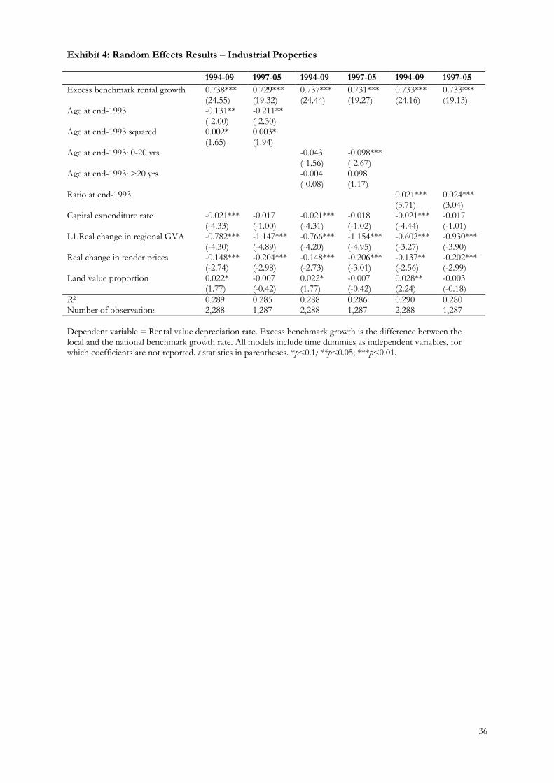
Exhibit 4: Random Effects Results – Industrial Properties
1994-09 1997-05 1994-09 1997-05 1994-09 1997-05 Excess benchmark rental growth 0.738*** 0.729*** 0.737*** 0.731*** 0.733*** 0.733*** (24.55) (19.32) (24.44) (19.27) (24.16) (19.13) Age at end-1993 -0.131** -0.211** (-2.00) (-2.30) Age at end-1993 squared 0.002* 0.003* (1.65) (1.94) Age at end-1993: 0-20 yrs -0.043 -0.098*** (-1.56) (-2.67) Age at end-1993: >20 yrs -0.004 0.098 (-0.08) (1.17) Ratio at end-1993 0.021*** 0.024*** (3.71) (3.04) Capital expenditure rate -0.021*** -0.017 -0.021*** -0.018 -0.021*** -0.017 (-4.33) (-1.00) (-4.31) (-1.02) (-4.44) (-1.01) L1.Real change in regional GVA -0.782*** -1.147*** -0.766*** -1.154*** -0.602*** -0.930*** (-4.30) (-4.89) (-4.20) (-4.95) (-3.27) (-3.90) Real change in tender prices -0.148*** -0.204*** -0.148*** -0.206*** -0.137** -0.202*** (-2.74) (-2.98) (-2.73) (-3.01) (-2.56) (-2.99) Land value proportion 0.022* -0.007 0.022* -0.007 0.028** -0.003 (1.77) (-0.42) (1.77) (-0.42) (2.24) (-0.18) R2 0.289 0.285 0.288 0.286 0.290 0.280 Number of observations 2,288 1,287 2,288 1,287 2,288 1,287 Dependent variable = Rental value depreciation rate. Excess benchmark growth is the difference between the local and the national benchmark growth rate. All models include time dummies as independent variables, for which coefficients are not reported. t statistics in parentheses. *p<0.1; **p<0.05; ***p<0.01.
36

Exhibit 5: Between Effects Results – Office Properties
1994-09 1997-05 1994-09 1997-05 1994-09 1997-05 Excess benchmark rental growth 0.232*** 0.521*** 0.245*** 0.544*** 0.104* 0.443*** (3.45) (7.89) (3.59) (8.18) (1.77) (6.97) Age at end-1993 -0.019*** -0.038*** (-2.62) (-3.61) Age at end-1993 squared 0.0001** 0.0002*** (2.30) (3.01) Age at end-1993: 0-40 yrs -0.022** -0.056*** (-2.11) (-3.81) Age at end-1993: >40 yrs 0.002 0.007 (0.51) (1.16) Ratio at end-1993 0.027*** 0.025*** (7.42) (4.71) Log floorspace 0.051 -0.034 0.069 0.009 0.207 0.215 (0.34) (-0.17) (0.46) (0.05) (1.63) (1.14) Capital expenditure rate -0.021 -0.128** -0.023 -0.122** -0.082** -0.191*** (-0.53) (-2.39) (-0.59) (-2.28) (-2.31) (-3.65) Land value proportion -0.049*** -0.072*** -0.051*** -0.074*** -0.024** -0.064*** (-4.29) (-5.03) (-4.48) (-5.18) (-2.25) (-4.53) Intercept 2.261 3.725** 2.231* 3.642** -2.079* -0.969 (1.53) (2.10) (1.76) (2.06) (-1.71) (-0.53) R2 0.143 0.336 0.135 0.343 0.305 0.361 Number of properties 206 206 206 206 206 206 Dependent variable = Rental value depreciation rate. Excess benchmark growth is the difference between the local and the national benchmark growth rate. t statistics in parentheses. *p<0.1; **p<0.05; ***p<0.01.
37

Exhibit 6: Between Effects Results – Industrial Properties
1994-09 1997-05 1994-09 1997-05 1994-09 1997-05 Excess benchmark rental growth 0.419*** 0.368*** 0.417*** 0.373*** 0.518*** 0.477*** (3.80) (4.12) (3.77) (4.18) (5.43) (5.42) Age at end-1993 -0.041 -0.130** (-0.97) (-2.17) Age at end-1993 squared 0.0003 0.003* (0.28) (1.74) Age at end-1993: 0-20 yrs -0.032 -0.077** (-1.46) (-2.46) Age at end-1993: >20 yrs -0.024 0.058 (-0.66) (1.13) Ratio at end-1993 0.025*** 0.027*** (7.14) (4.80) Log floorspace 0.248* 0.142 0.250* 0.148 0.081 0.041 (1.65) (0.66) (1.65) (0.69) (0.61) (0.20) Capital expenditure rate -0.131 -0.169 -0.130 -0.171 -0.141* -0.185* (-1.50) (-1.57) (-1.49) (-1.59) (-1.87) (-1.83) Land value proportion -0.023** -0.067*** -0.023** -0.067*** -0.003 -0.049*** (-2.28) (-4.96) (-2.28) (-4.96) (-0.36) (-3.64) Intercept -1.196 0.623 -1.253 0.387 -2.624** -2.115 (-0.86) (0.31) (-0.91) (0.20) (-2.34) (-1.19) R2 0.216 0.327 0.216 0.330 0.412 0.400 Number of properties 143 143 143 143 143 143 Dependent variable = Rental value depreciation rate. Excess benchmark growth is the difference between the local and the national benchmark growth rate. t statistics in parentheses. *p<0.1; **p<0.05; ***p<0.01.
38
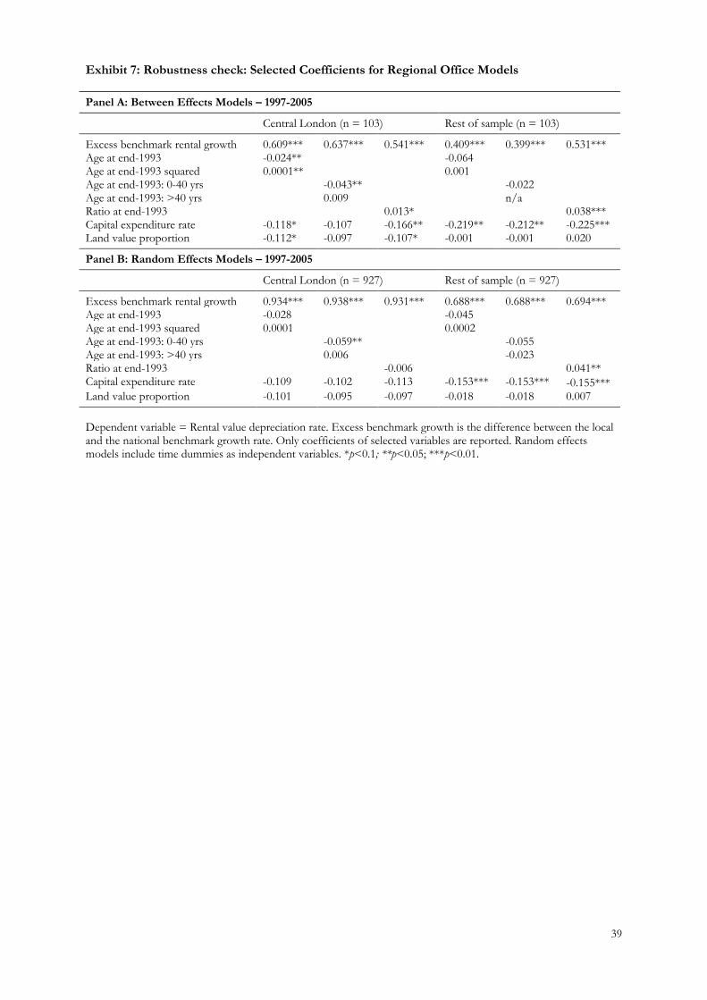
Exhibit 7: Robustness check: Selected Coefficients for Regional Office Models
Panel A: Between Effects Models – 1997-2005
Central London (n = 103) Rest of sample (n = 103)
Excess benchmark rental growth 0.609*** 0.637*** 0.541*** 0.409*** 0.399*** 0.531*** Age at end-1993 -0.024** -0.064 Age at end-1993 squared 0.0001** 0.001 Age at end-1993: 0-40 yrs -0.043** -0.022 Age at end-1993: >40 yrs 0.009 n/a Ratio at end-1993 0.013* 0.038*** Capital expenditure rate -0.118* -0.107 -0.166** -0.219** -0.212** -0.225*** Land value proportion -0.112* -0.097 -0.107* -0.001 -0.001 0.020
Panel B: Random Effects Models – 1997-2005
Central London (n = 927) Rest of sample (n = 927)
Excess benchmark rental growth 0.934*** 0.938*** 0.931*** 0.688*** 0.688*** 0.694*** Age at end-1993 -0.028 -0.045 Age at end-1993 squared 0.0001 0.0002 Age at end-1993: 0-40 yrs -0.059** -0.055 Age at end-1993: >40 yrs 0.006 -0.023 Ratio at end-1993 -0.006 0.041** Capital expenditure rate -0.109 -0.102 -0.113 -0.153*** -0.153*** -0.155*** Land value proportion -0.101 -0.095 -0.097 -0.018 -0.018 0.007 Dependent variable = Rental value depreciation rate. Excess benchmark growth is the difference between the local and the national benchmark growth rate. Only coefficients of selected variables are reported. Random effects models include time dummies as independent variables. *p<0.1; **p<0.05; ***p<0.01.
39

Exhibit 8: Robustness check: Selected Between Effects and Random Effects Office Models
Without control for land value proportion (1997-2005)
Without office properties older than 50 years (1997-2005)
Between Effects
Random Effects
Between Effects
Random Effects
Excess benchmark growth 0.468*** 0.687*** 0.487*** 0.646*** Age at end-1993 -0.053*** -0.045*** -0.125** -0.224* Age at end-1993 squared 0.0002*** 0.0001** 0.002 0.003 Capital expenditure rate 0.122** -0.113* -0.113* -0.082* Land value proportion -0.078*** -0.052** Dependent variable = Rental value depreciation rate. Excess benchmark growth is the difference between the local and the national benchmark growth rate. Only coefficients of selected variables are reported. Random effects models include time dummies as independent variables. *p<0.1; **p<0.05; ***p<0.01.
40
Top Related