


Languages
Pages
Legal


Statistics can be applied across most disciplines of study.
Statistics
Chemo-
metrics
Genetics
Psycho-
metrics
Medical
statistics
Image
process-
ing
Econo-
metrics
Epidemiology
Geostatistics
Actuarial
science
Where to use Statistics • It can be used in almost every phase of human
activity. – For example, in genetics, economics, insurance, finance,
medical studies, psychology, earth science, image
processing, graphical modeling, and so on.

2
Where to use Statistics
Statistical techniques are used to address a variety of
problems from, say finance.
2
• Build a financial model, and do estimation/make an
inference of financial models of bonds and stock prices.

3
Where to use Statistics
• Public Health --- Disease Outbreak (Disease
Clustering) Detection
• Early detection of disease outbreaks enables public health officials to
implement disease control and prevention measures at the earliest possible
time.
• Basic idea is to scan the target area (and time) to find regions with disease
count higher than expected.
3

4
Where to use Statistics
• Computer Science/Engineering --- Sign/Image
processing, machine learning, etc.
4
• Machine learning --- pattern recognition, classification
build a model from example inputs in order to make data-driven
predictions or decisions.
In classification, inputs are divided into two
or more classes, and the learner must
produce a model/FUNCTION that assigns
new or unseen inputs to one (or multi-label
classification) or more of these classes.

Example of Machine Learning
5
AlphaGo

6
Where to use Statistics
• Education ---agreement
6
** Kappa statistic should be introduced to assess the (inter-rater) agreement
between two different markers.

7
Where to use Statistics
• Bioinformatics --- the application of computer technology to the
management of biological information
7
• In many bioinformatics problems the number of features amounts to
several thousands: for example in cancer classification tasks the number
of variables (i.e. the number of genes for which expression is measured)
may range from 6,000 to 60,000.
Feature selection is indeed a typical statistical model (or variable) selection
problem.

8
Where to use Statistics
• Chemistry --- quality control, longitudinal data
8
Interpretation of quality control data involves both graphical and statistical
methods
The control charts: a statistical approach to the study of manufacturing
process variation for the purpose of improving the economic effectiveness of
the process. These methods are based on continuous monitoring of process
variation.

9

10

11
It is generally impossible or impractical to examine the entire
population, but we may examine a part of it (a sample from it) so
that we can find out something (say, population mean) about the
target population from the sample (say, use the sample mean) ---
making a statistical inference regarding the entire (unknown)
population.
Why do we need to draw a sample? Why do
we want a statistic, like sample mean?

Two branches of statistics
12

(i) Descriptive Procedure
13

(i) Descriptive Procedure
14

Two branches of statistics
15

(ii) Inferential Procedure
16

(ii) Inferential Procedure
17

Chapter One
(1) Descriptive Statistics
18

1. What are DATA?
19
Data (its singular form is datum) in science
are a collection of measurements and
identifiers. These can take many forms like
numerical, character, or any other form of
output.

20
Note that in this table each row represents all measurements for a SINGLE case/patient.
Each column refers to a characteristic of our interest which we often call a variable.
Each datum (the value of a single variable for a single case) is also known as an observation.
Data summarization: Note that data without summarizing like
35, 42, 21, 59, 47, 55, 55, 38, 50, 41, 51, 44, 31, 42, 30, 32, 40, F, F, M, ………
are completely meaningless and non-informative.
Consider the following data extracted from medical records of 50 patients with low back pain:
Subject Age Gender In employment? Duration of pain Severity of
pain First episode of pain
1 35 F No 3 weeks Mild < 1 year
2 42 F Yes 13 weeks Severe 1-6 years
3 21 M Yes 4 weeks Moderate < 1 year
4 59 F No 72 weeks Moderate ≥ 11 years
⋮ ⋮ ⋮ ⋮ ⋮ ⋮ ⋮
50 40 M Yes 30 weeks severe 6-11 years
How to summarize these data?
Different variables require different methods
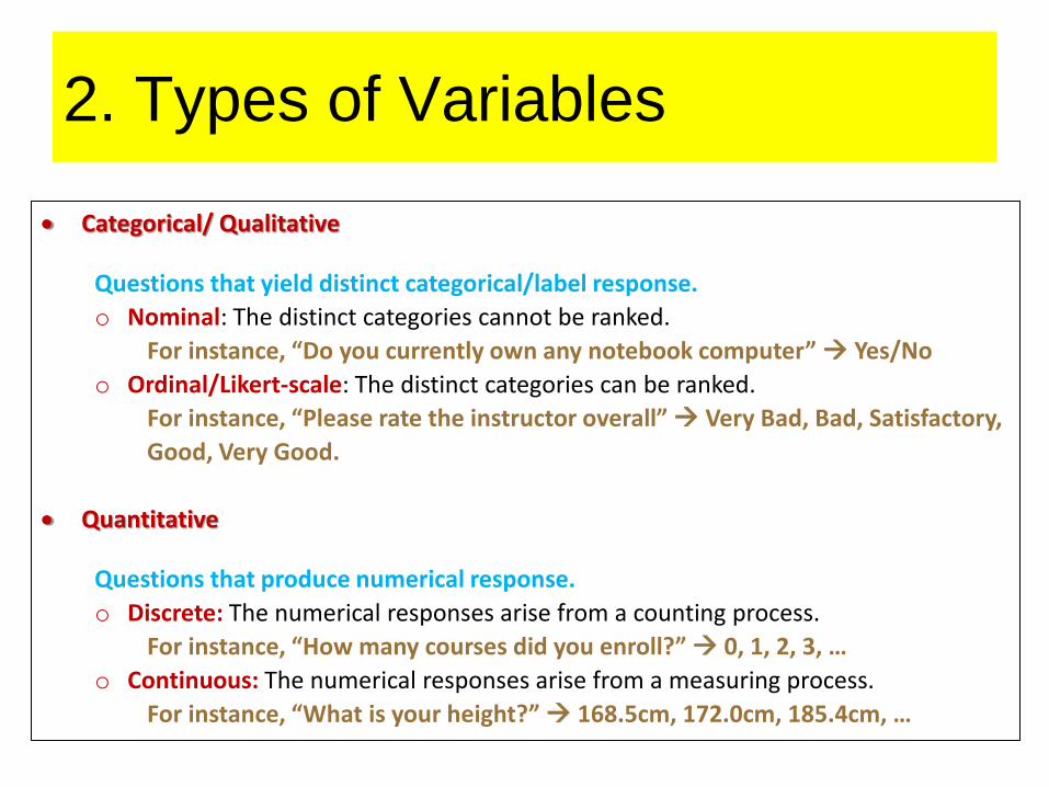
2. Types of Variables
Categorical/ Qualitative
Questions that yield distinct categorical/label response.
o Nominal: The distinct categories cannot be ranked.
For instance, “Do you currently own any notebook computer” Yes/No
o Ordinal/Likert-scale: The distinct categories can be ranked.
For instance, “Please rate the instructor overall” Very Bad, Bad, Satisfactory,
Good, Very Good.
Quantitative
Questions that produce numerical response.
o Discrete: The numerical responses arise from a counting process.
For instance, “How many courses did you enroll?” 0, 1, 2, 3, …
o Continuous: The numerical responses arise from a measuring process.
For instance, “What is your height?” 168.5cm, 172.0cm, 185.4cm, …

22
WHY SHOULD WE CARE ABOUT THE TYPE OF VARIABLE?
Note that in practice categorical variables are often recorded using numbers (e.g. yes = 1, no = 0). Please don’t mistake these for quantitative variables.
Thus, knowing the type of variables can help
• Decide how to interpret the data from variable. For instance, if a measure is nominal, then the numerical values are just short
codes for the longer names. • Decide what statistical analysis is appropriate on the values that were assigned.
For instance, if a measure is ordinal (like strongly disagree, disagree, neutral, agree, strongly agree), then averaging such data values is INCORRECT/ INVALID. Median or proportion should be used.
Fuzzy Statistics is a relatively new approach to analyze ordinal/Likert-scale data

3. Data presentation
(Tabular and Graphical)
23

3.1 Frequency Table
24
Procedure:
i. Selects an appropriate number of class intervals. Normally use 5 - 20 classes.
ii. Obtains a suitable class intervals by dividing the range of the data by the number decided
at the previous step.
iii. Establishes the boundaries of each class to avoid overlapping.
iv. Construct a table with columns of the class interval, class midpoint, and class frequency.

3.2 Histogram
25

3.3 Boxplot
26

27
How to get the quartiles of the data?

28
Boxplot is commonly used to detect the
so-called outliers (unusual data points) which
may be produced by measurement error and
occurs with a small probability. Normally, outliers
are far away from the majority of the data.
The data point is labeled to be an outlier if its value is
o ≤ Q1 - 1.5IQR OR
o ≥ Q3 + 1.5IQR
According to this rule with the value 1.5, if the data are from
the normal distribution, we can show that there is a 0.0076
chance that the data points fall into the above regions.

Data are the daily closing price of the S&P 500 Index from 3rd January 2000 to 2nd December 2011.
29
Side-by-side Boxplot for grouped data

30

4. Data presentation
(Numerical)
31
Suppose that we have n data labeled by x1, x2, …, xn.

4.1 Center
32

33
0
0
0 110
22

4.2 Spread or Dispersion
34

35

Software: R
36
Throughout this course, we would also study how to use an open-source
software R to analyze data
R installation:

Read External Data with R
1) Save data set on your computer;
3) Change the directory by clicking on [File] at the top left
and then choosing the option for [Change dir].
2) Open R;
37

38

39

40

Double click
41

42

43

44
An important R function used to read a data set:
read.table(): read a data set having 2 or more variables.
Read External Data with R

Caution!!
Head(er) or not in the 1st row?!?!
With Header:
read.table(“test1.txt", header=T) x =
Without Header:
read.table(“test1.txt", header=F) x =
45
Read External Data with R

Separation ? read.table( )
read.table(“test1.txt”, header = F, sep = “”, …..)
sep: the field separator character that separates values on each line of the file.
25 28 14
26 29 28
27 22 30
28 31 27
29 25 33
30 20 11
Separated by one or more spaces.
sep=“” (default setting)
No space
46

Separation ? read.table( )
read.table(“test2.txt”, header = F, …..)
sep: the field separator character that separate values on each line of the file.
25,28,14
26,29,28
27,22,30
28,31,27
29,25,33
30,20,11
Separated by commas.
sep=“,”
47

Separation ? read.table( )
read.table(“test3.txt”, header = F, …..)
sep: the field separator character that separate values on each line of the file.
25 28 14
26 29 28
27 22 30
28 31 27
29 25 33
30 20 11
Separated by tabs.
sep=“\t”
48

Real Data Set
49
The data set (BGSall.txt) contains data from the Berkeley guidance study of
children born in 1928-29 in Berkeley, CA.
Variables
Sex 0 = males, 1 = females
WT2 Age 2 weight (kg)
HT2 Age 2 height (cm)
WT9 Age 9 weight (kg)
HT9 Age 9 height (cm)
LG9 Age 9 leg circumference (cm)
ST9 Age 9 strength (kg)
WT18 Age 18 weight (kg)
HT18 Age 18 height (cm)
LG18 Age 18 leg circumference (cm)
ST18 Age 18 strength (kg)
Soma Somatotype, a 1 to 7 scale of body type.

50
In the following, we would like to summarize the data for WT9.

51
z1[,2] is a vector of data for WT9
Sex
0 = males, 1 = females
By Gender

Frequency Table with R
52
The frequency table of a data is a summary of the data occurrence in a
collection of non-overlapping categories.
1. We first find the range of WT9 with the range function. It shows that the
observed weights are between 19.9 and 66.8 kg.
2. Break the range into non-overlapping sub-intervals (say 10) by defining a
sequence of equal distance break points. If we round the endpoints of the
interval [19.9, 66.8] to the closest half-integers, we come up with the interval
[19.5, 67]. Hence, the common length of the break points is
and the break points are the sequence { 19.5, 24.25, 29, ... }.

Frequency Table with R
53
The frequency table of a data is a summary of the data occurrence in a
collection of non-overlapping categories.
3. Classify the data according to the sub-intervals with cut. As the intervals are
to be closed on the left, and open on the right, we set the right argument as
FALSE.
4. Compute the frequency of the data in each sub-interval with the table
function.

54
5. We apply the cbind function to print the result in column format.
Frequency Table with R
The frequency table of a data is a summary of the data occurrence in a
collection of non-overlapping categories.
wtcut = cut(z1$WT9, breaks = bp, right=FALSE, dig.lab = 4)

55
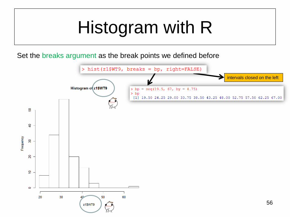
We apply the hist function to produce the histogram of WT9.
Histogram with R
A histogram consists of parallel vertical bars that graphically shows the
frequency table of data. The area of each bar is equal to the frequency of data
found in each category.
56
Histogram with R
Set the breaks argument as the break points we defined before
intervals closed on the left

57
To colorize the histogram, we select a color palette and set it in the col
argument of hist. In addition, we update the titles for readability.
Histogram with R

58
pm = hist(subset(z1$WT9, z1$Sex == 0), breaks = bp, right=FALSE) pf = hist(subset(z1$WT9, z1$Sex == 1), breaks = bp, right=FALSE)
Histogram with R
Compare the weights of male and female with histogram.
plot(pm, col=rgb(0, 0, 1, 0.3), main="Histogram of Weight at age of 9 by Gender", xlab="Weight (kg)") plot(pf, col=rgb(1, 0, 0, 0.3), add=T)

59
Which is for boys,
which is for girls?

60
pm = hist(subset(z1$WT9, z1$Sex == 0), breaks = bp, right=FALSE) pf = hist(subset(z1$WT9, z1$Sex == 1), breaks = bp, right=FALSE)
Histogram with R
Compare the weights of male and female with histogram.
plot(pm, col=rgb(0, 0, 1, 0.3), main="Histogram of Weight at age of 9 by Gender", xlab="Weight (kg)") plot(pf, col=rgb(1, 0, 0, 0.3), add=T)
legend("topright", c("Male", "Female"), col=c(rgb(0,0, 1, 0.3), rgb(1,0,0, 0.3)), lwd=10)

61
par(mfrow = c(2, 1)) plot(pm, col=rgb(0, 0, 1, 0.3), main="Histogram of Weight at age of 9 \n for boys", xlab="Weight (kg)") plot(pf, col=rgb(1, 0, 0, 0.3), main="Histogram of Weight at age of 9 \n for girls", xlab="Weight (kg)")
I know which is for
boys and which is
for girls!!
par(mfrow = c(r, c))
Produce two separate
histograms in a single frame

62

Boxplot with R
63
Top Related