


![Jacob Anderskov Habitable Exomusics] - The trilogyjacobanderskov.dk/.../05/JA_Habitable_Exomusics_TheTrilogy_Press… · Habitable Exomusics, refers to “habitable exoplanets”,](https://static.fdocuments.us/doc/165x107/5f077b3d7e708231d41d3244/jacob-anderskov-habitable-exomusics-the-t-habitable-exomusics-refers-to-aoehabitable.jpg)
Languages
Pages
Legal


Water vapour in the atmosphere of the habitable-zone eight
Earth-mass planet K2-18 b
Angelos Tsiaras1,∗, Ingo P. Waldmann1, Giovanna Tinetti1, Jonathan Tennyson1 & Sergey N. Yurchenko1
1Department of Physics & Astronomy, University College London, Gower Street, WC1E 6BT London, UK
∗Corresponding author
In the past decade, observations from space and ground have found H2O to be the most1
abundant molecular species, after hydrogen, in the atmospheres of hot, gaseous, extrasolar2
planets1–5. Being the main molecular carrier of oxygen, H2O is a tracer of the origin and3
the evolution mechanisms of planets. For temperate, terrestrial planets, the presence of H2O4
is of great significance as an indicator of habitable conditions. Being small and relatively5
cold, these planets and their atmospheres are the most challenging to observe, and there-6
fore no atmospheric spectral signatures have so far been detected6. Super-Earths – planets7
lighter than ten M⊕ – around later-type stars may provide our first opportunity to study8
spectroscopically the characteristics of such planets, as they are best suited for transit obser-9
vations. Here we report the detection of an H2O spectroscopic signature in the atmosphere10
of K2-18 b – an eight M⊕ planet in the habitable-zone of an M-dwarf7 – with high statistical11
confidence (ADI5 = 5.0, ∼3.6σ8, 9). In addition, the derived mean molecular weight suggests12
an atmosphere still containing some hydrogen. The observations were recorded with the13
Hubble Space Telescope/WFC3 camera, and analysed with our dedicated, publicly avail-14
1

able, algorithms5, 9. While the suitability of M-dwarfs to host habitable worlds is still under15
discussion10–13, K2-18 b offers an unprecedented opportunity to get insight into the composi-16
tion and climate of habitable-zone planets.17
Atmospheric characterisation of super-Earths is currently within reach of the Wide Field18
Camera 3 (WFC3) onboard the Hubble Space Telescope (HST), combined with the recently im-19
plemented spatial scanning observational strategy14. The spectra of three hot transiting planets20
with radii less than 3.0 R⊕ have been published so far: GJ-1214 b15, HD 97658 b16 and 55 Cnc e17.21
The first two do not show any evident transit depth modulation with wavelength, suggesting an at-22
mosphere covered by thick clouds or made of molecular species heavier than hydrogen, while only23
the spectrum of 55 Cnc e has revealed a light-weighted atmosphere, suggesting H/He still being24
present. In addition, transit observations of six temperate Earth-size planets around the ultra-cool25
dwarf TRAPPIST-1 – planets b, c, d, e, f6, and g18 – have not shown any molecular signatures and26
have excluded the presence of cloud-free, H/He atmospheres around them.27
K2-18 b was discovered in 2015 by the Kepler spacecraft7, and it is orbiting around an28
M2.5 ([Fe/H] = 0.123 ± 0.157 dex, Teff = 3457 ± 39K, M∗ = 0.359 ± 0.047M�, R∗ =29
0.411±0.038R�)19 dwarf star, 34 pc away from the Earth. The star-planet distance of 0.1429 AU1930
suggests a planet within the star’s habitable zone (∼ 0.12 – 0.25 AU)20, with effective temperature31
between 200 K and 320 K, depending on the albedo and the emissivity of its surface and/or its at-32
mosphere. This crude estimate accounts for neither possible tidal energy sources21 nor atmospheric33
heat redistribution11, 13, which might be relevant for this planet. Measurements of the mass and the34
2

radius of K2-18 b (Mp = 7.96 ± 1.91M⊕22, Rp = 2.279 ± 0.0026R⊕
19) yield a bulk density35
of 3.3±1.2 g/cm22, suggesting either a silicate planet with an extended atmosphere around or an36
interior composition with an H2O mass fraction lower that 50%22–24.37
We analyse here eight transits of K2-18 b obtained with the WFC3 camera onboard the Hub-38
ble Space Telescope. We used our specialised, publicly available, tools5, 9 to perform the end-to-39
end analysis from the raw HST data to the atmospheric parameters. The accuracy of the techniques40
used here have been demonstrated through the largest consistently analysed catalogue of exoplan-41
etary spectra from WFC35. Details on the data analysis can be found in the Methods section. Also,42
links to the data and the codes used can be found in the Data availability and Code availability43
sections, respectively. Alongside with the data we provide descriptions of the data structures and44
instructions on how to reproduce the results presented here. Our analysis resulted in the detection45
of an atmosphere around K2-18 b with an ADI5 (a positively defined logarithmic Bayes Factor)46
of 5.0, or approximately 3.6σ confidence8, 9, making K2-18 b the first habitable-zone planet in the47
super-Earth mass regime (1-10 M⊕) with an observed atmosphere around it.48
More specifically, nine transits of K2-18 b were observed as part of the HST proposals 1366549
and 14682 (PI: Bjorn Benneke) and the data are available through the MAST Archive (see Data50
Availability section). Each transit was observed during five HST orbits, with the G141 infrared51
grism (1.1 - 1.7µm), and each exposure was the result of 16 up-the-ramp samples in the spatially52
scanning mode. The ninth transit observation suffered from pointing instabilities and therefore we53
decided not to include it in this analysis. We extracted the white and the spectral light curves from54
3
the reduced images, following our dedicated methodology5, 17, 25, which has been integrated into an55
automated, self-consistent, and user-friendly Python package named Iraclis (see Code Availability56
section). No systematic variations of the white light-curve Rp/R∗ appeared between the eight57
different observations. This level of stability among the extracted broad-band transit depths is not58
always guaranteed, as consistency problems among different observations emerged in previous59
analyses5, 16.60
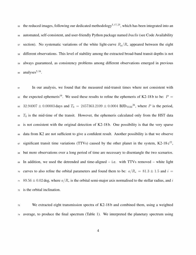
In our analysis, we found that the measured mid-transit times where not consistent with61
the expected ephemeris19. We used these results to refine the ephemeris of K2-18 b to be: P =62
32.94007 ± 0.00003 days and T0 = 2457363.2109 ± 0.0004 BJDTDB26, where P is the period,63
T0 is the mid-time of the transit. However, the ephemeris calculated only from the HST data64
is not consistent with the original detection of K2-18 b. One possibility is that the very sparse65
data from K2 are not sufficient to give a confident result. Another possibility is that we observe66
significant transit time variations (TTVs) caused by the other planet in the system, K2-18 c22,67
but more observations over a long period of time are necessary to disentangle the two scenarios.68
In addition, we used the detrended and time-aligned – i.e. with TTVs removed – white light69
curves to also refine the orbital parameters and found them to be: a/R∗ = 81.3 ± 1.5 and i =70
89.56± 0.02 deg, where a/R∗ is the orbital semi-major axis normalised to the stellar radius, and i71
is the orbital inclination.72
We extracted eight transmission spectra of K2-18 b and combined them, using a weighted73
average, to produce the final spectrum (Table 1). We interpreted the planetary spectrum using74
4

our spectral retrieval algorithm TauREx9, 27 (see Code Availability section) which combines highly75
accurate line lists28 (see Data Availability section) and Bayesian analysis. At an initial stage, we76
modelled the atmosphere of K2-18 b including all potential absorbers in the observed wavelength77
range – i.e. H2O, CO, CO2, CH4 and NH3. However, we found that only the spectroscopic signa-78
ture of water vapour is detected with high-confidence, so we continued our analysis only with this79
molecule as trace-gas. We modelled the atmosphere following three approaches:80
• a cloud-free atmosphere containing only H2O and H2/He81
• a cloud-free atmosphere containing H2O, H2/He and N2 (N2 acted as proxy for “invisible”82
molecules not detectable in the WFC3 bandpass but contributing to the mean molecular83
weight), and84
• a cloudy (flat-line model) atmosphere containing only H2O and H2/He.85
We retrieved a statistically significant atmosphere around K2-18 b in all simulations (Figure86
3), and assessed the strength of the detection using the Atmospheric Detectability Index5 (ADI),87
which represents the positively defined logarithmic Bayes Factor, where the null hypothesis is a88
model that contains no active trace gases, Rayleigh scattering or collision induced absorption – i.e.89
a flat spectrum. The retrieval simulations yield an atmospheric detection with an ADI of 5.0, 4.790
and 4.0, respectively. Such ADIs correspond to approximately a 3.6, 3.5, and 3.3 σ detection8, 9,91
respectively. This marks the first atmosphere detected around a habitable-zone super-Earth with92
such a high level of confidence. While the H2O + H2/He case appears to be the most favourable,93
5

this preference is not statistically significant.94
As far as the composition is concerned, retrieval models confirm the presence of water vapour95
in the atmosphere of K2-18 b in all the cases studied with high statistical significance. However, it96
is not possible to constrain either its abundance or the mean molecular weight of the atmosphere.97
For the H2O + H2/He case, we found the abundance of H2O to be between 50% and 20%, while98
for the other two cases between 0.01% and 12.5%. The atmospheric mean molecular weight can99
be between 5.8 and 11.5 amu in the H2O + H2/He case, and between 2.3 and 7.8 amu for the other100
cases. These results indicate that a non-negligible fraction of the atmosphere is still made of H/He.101
Additional trace-gases – e.g. CH4, NH3 – cannot be excluded, despite not being identified with the102
current observations: the limiting S/N and wavelength coverage of HST/WFC3 do not allow the103
detection of other molecules.104
The results presented here confirm the existence of a detectable atmosphere around K2-18 b,105
making it one of the most interesting known targets for further atmospheric characterisation with106
future observatories, like the James Webb Space Telescope (0.6µm and 28µm) and the European107
Space Agency ARIEL mission29 (0.5µm and 7.8µm). The wider wavelength coverage of these108
instruments will provide information on the presence of additional molecular species and on the109
temperature-pressure profile of the planet, towards studying the planetary climate and potential110
habitability. While the subject of habitability for temperate planets around late-type stars is a111
subject of active discussion10–13 and real progress requires significantly improved observational112
constraints, the analysis presented here provides the first direct observation of a molecular signature113
6

from a habitable-zone exoplanet, connecting these theoretical studies to observations.114
115 1. Tinetti, G. et al. Infrared Transmission Spectra for Extrasolar Giant Planets. Astrophys. J.116
Lett. 654, L99–L102 (2007).117
2. Grillmair, C. J. et al. Strong water absorption in the dayside emission spectrum of the planet118
HD189733b. Nature 456, 767-769 (2008).119
3. Fraine, J. et al. Water vapour absorption in the clear atmosphere of a Neptune-sized exoplanet.120
Nature 350, 64-67 (2015).121
4. Macintosh, B. et al. Discovery and spectroscopy of the young jovian planet 51 Eri b with the122
Gemini Planet Imager. Science 456, 767-769 (2008).123
5. Tsiaras, A. et al. A Population Study of Gaseous Exoplanets. Astron. J. 155 (2018).124
6. de Wit, J. et al. Atmospheric reconnaissance of the habitable-zone Earth-sized planets orbiting125
TRAPPIST-1. Nat. Astron. 2, 214–219 (2018)126
7. Montet, B. T. et al. Stellar and Planetary Properties of K2 Campaign 1 Candidates and Vali-127
dation of 17 Planets, Including a Planet Receiving Earth-like Insolation. Astrophys. J. 809, 25128
(2015).129
8. Benneke, B. & Seager, S. How to Distinguish between Cloudy Mini-Neptunes and130
Water/Volatile-dominated Super-Earths. Astrophys. J. 778, 153 (2013).131
7

9. Waldmann, I. P. et al. Tau-REx I: A Next Generation Retrieval Code for Exoplanetary Atmo-132
spheres. Astrophys. J. 802, 107 (2015).133
10. Segura, A. et al. Biosignatures from Earth-Like Planets Around M Dwarfs. Astrobiology 5,134
706–725 (2005).135
11. Wordsworth, R. D. et al. Gliese 581d is the First Discovered Terrestrial-mass Exoplanet in the136
Habitable Zone. Astrophys. J. 733, L48 (2011).137
12. Leconte, J. et al. 3D climate modeling of close-in land planets: Circulation patterns, climate138
moist bistability, and habitability. Astron. Astrophys. 554, A69 (2013).139
13. Turbet, M. et al. The habitability of Proxima Centauri b. II. Possible climates and observabil-140
ity. Astron. Astrophys. 596, A112 (2016).141
14. Deming, D. et al. Infrared Transmission Spectroscopy of the Exoplanets HD 209458b and142
XO-1b Using the Wide Field Camera-3 on the Hubble Space Telescope. Astrophys. J. 774, 95143
(2013).144
15. Kreidberg, L. et al. Clouds in the atmosphere of the super-Earth exoplanet GJ1214b. Nature145
505, 69–72 (2014).146
16. Knutson, H. A. et al. Hubble Space Telescope Near-IR Transmission Spectroscopy of the147
Super-Earth HD 97658b. Astrophys. J. 794, 155 (2014).148
17. Tsiaras, A. et al. Detection of an Atmosphere Around the Super-Earth 55 Cancri e. Astrophys.149
J. 820, 99 (2016).150
8

18. Wakeford, H. R et al. Disentangling the Planet from the Star in Late-Type M Dwarfs: A Case151
Study of TRAPPIST-1g. Astron. J. 157, 11 (2019).152
19. Benneke, B. et al. Spitzer Observations Confirm and Rescue the Habitable-zone Super-Earth153
K2-18b for Future Characterization. Astrophys. J. 834, 187 (2017).154
20. Kopparapu, R. K. A Revised Estimate of the Occurrence Rate of Terrestrial Planets in the155
Habitable Zones around Kepler M-dwarfs. Astrophys. J. Lett. 767, L8 (2013).156
21. Valencia, D., Tan, V. Y. Y. & Zajac, Z. Habitability from Tidally Induced Tectonics. Astrophys.157
J. 857, 106 (2018).158
22. Cloutier, R. et al. Characterization of the K2-18 multi-planetary system with HARPS. A159
habitable zone super-Earth and discovery of a second, warm super-Earth on a non-coplanar160
orbit. Astron. Astrophys. 608, A35 (2017).161
23. Valencia, D., Guillot, T., Parmentier, V. & Freedman, R. S. Bulk Composition of GJ 1214b162
and Other Sub-Neptune Exoplanets. Astrophys. J. 775, 10 (2013).163
24. Zeng, L., Sasselov, D. D. & Jacobsen, S. B. Mass-Radius Relation for Rocky Planets Based164
on PREM. Astrophys. J. 819, 127 (2016).165
25. Tsiaras, A. et al. A New Approach to Analyzing HST Spatial Scans: The Transmission166
Spectrum of HD 209458 b. Astrophys. J. 832, 202 (2016).167
26. Eastman, J. et al. Achieving Better Than 1 Minute Accuracy in the Heliocentric and Barycen-168
tric Julian Dates. Publ. Astron. Soc. Pac. 122, 935 (2010).169
9

27. Waldmann, I. P. et al. Tau-REx II: Retrieval of Emission Spectra. Astrophys. J. 813, 13 (2015).170
28. Tennyson, J. et al. The ExoMol database: Molecular line lists for exoplanet and other hot171
atmospheres. J. Mol. Spec. 327, 73–94 (2016).172
29. Tinetti, G. et al. A chemical survey of exoplanets with ARIEL. Exp. Astron. 46, 135–209173
(2018).174
Acknowledgements This project has received funding from the European Research Council175
(ERC) under the European Union’s Horizon 2020 research and innovation programme (grant176
agreements 758892, ExoAI; 776403/ExoplANETS A) and under the European Union’s Seventh177
Framework Programme (FP7/2007-2013)/ ERC grant agreement numbers 617119 (ExoLights) and178
267219 (ExoMol). We furthermore acknowledge funding by the Science and Technology Funding179
Council (STFC) grants: ST/K502406/1 and ST/P000282/1. The data used here were obtained by180
the Hubble Space Telescope as part of the 13665 and 14682 GO proposals (PI: Bjorn Benneke).181
Author Contributions A.T. performed the data analysis and developed the HST analysis soft-182
ware Iraclis; I.P.W developed the atmospheric retrieval software TauREx; G.T. contributed to the183
interpretation of the results; J.T. and S.N.Y. coordinate the ExoMol project. All authors discussed184
the results and commented on the manuscript.185
Financial Interests The authors declare no competing financial interests.186
10

Materials & Correspondence Correspondence and requests for materials should be addressed187
to A.T. ([email protected]) or I.P.W. ([email protected]).188
11

−0.004
−0.002
0.000
0.002
0.004
0.006
phase
0.960
0.965
0.970
0.975
0.980
0.985
0.990
0.995
1.000
norm
.flux
1.1560μm
1.1885μm
1.2185μm
1.2470μm
1.2750μm
1.3025μm
1.3290μm
1.3555μm
1.3825μm
1.4095μm
1.4365μm
1.4640μm
1.4920μm
1.5200μm
1.5480μm
1.5765μm
1.6055μm
white
1.1560μm
1.1885μm
1.2185μm
1.2470μm
1.2750μm
1.3025μm
1.3290μm
1.3555μm
1.3825μm
1.4095μm
1.4365μm
1.4640μm
1.4920μm
1.5200μm
1.5480μm
1.5765μm
1.6055μm
white
1.1560μm
1.1885μm
1.2185μm
1.2470μm
1.2750μm
1.3025μm
1.3290μm
1.3555μm
1.3825μm
1.4095μm
1.4365μm
1.4640μm
1.4920μm
1.5200μm
1.5480μm
1.5765μm
1.6055μm
white
1.1560μm
1.1885μm
1.2185μm
1.2470μm
1.2750μm
1.3025μm
1.3290μm
1.3555μm
1.3825μm
1.4095μm
1.4365μm
1.4640μm
1.4920μm
1.5200μm
1.5480μm
1.5765μm
1.6055μm
white
1.1560μm
1.1885μm
1.2185μm
1.2470μm
1.2750μm
1.3025μm
1.3290μm
1.3555μm
1.3825μm
1.4095μm
1.4365μm
1.4640μm
1.4920μm
1.5200μm
1.5480μm
1.5765μm
1.6055μm
white
1.1560μm
1.1885μm
1.2185μm
1.2470μm
1.2750μm
1.3025μm
1.3290μm
1.3555μm
1.3825μm
1.4095μm
1.4365μm
1.4640μm
1.4920μm
1.5200μm
1.5480μm
1.5765μm
1.6055μm
white
1.1560μm
1.1885μm
1.2185μm
1.2470μm
1.2750μm
1.3025μm
1.3290μm
1.3555μm
1.3825μm
1.4095μm
1.4365μm
1.4640μm
1.4920μm
1.5200μm
1.5480μm
1.5765μm
1.6055μm
white
1.1560μm
1.1885μm
1.2185μm
1.2470μm
1.2750μm
1.3025μm
1.3290μm
1.3555μm
1.3825μm
1.4095μm
1.4365μm
1.4640μm
1.4920μm
1.5200μm
1.5480μm
1.5765μm
1.6055μm
white
de− trended
−0.004
−0.002
0.000
0.002
0.004
0.006
phase
1000 ppm1000 ppm1000 ppm1000 ppm1000 ppm1000 ppm1000 ppm
σ=1.09
σ=1.12
σ=1.07
σ=1.08
σ=1.16
σ=1.13
σ=1.09
σ=1.05
σ=1.17
σ=1.10
σ=1.01
σ=1.02
σ=1.04
σ=1.05
σ=1.02
σ=1.10
σ=1.14
σ=2.08
1000 ppm
residuals
Figure 1: Analysis of the K2-18 b white (black points) and spectral (coloured points) light curves,
plotted with an offset for clarity. Left: Overploted detrended light curves. Right: Overploted
fitted residuals, where σ indicates the ratio between the standard deviation of the residuals and the
photon noise (see Methods for more details). The black vertical bar indicates the 1000ppm scatter
level.12

Table 1: Transit depth ((Rp/R∗)2) for the different wavelength channels, where Rp is the
planetary radius, R∗ is the stellar radius, and λ1, λ2 are the lower and upper edges of each
wavelength channel, respectively.
λ1 λ2 (Rp/R∗)2
µm µm ppm
1.1390 1.1730 2905± 25
1.1730 1.2040 2939± 26
1.2040 1.2330 2903± 24
1.2330 1.2610 2922± 25
1.2610 1.2890 2891± 26
1.2890 1.3160 2918± 26
1.3160 1.3420 2919± 24
1.3420 1.3690 2965± 24
1.3690 1.3960 2955± 27
1.3960 1.4230 2976± 25
1.4230 1.4500 2990± 24
1.4500 1.4780 2895± 23
1.4780 1.5060 2930± 23
1.5060 1.5340 2921± 24
1.5340 1.5620 2875± 24
1.5620 1.5910 2927± 25
1.5910 1.6200 2925± 24
13

1.1 1.2 1.3 1.4 1.5 1.6Wavelength ( m)
2850
2875
2900
2925
2950
2975
3000
3025
3050
(Rp/R
*)2(p
pm)
H2O + cloudsH2O + N2
H2O onlyObserved
1.1 1.2 1.3 1.4 1.5 1.6Wavelength ( m)
2850
2875
2900
2925
2950
2975
3000
3025
3050
(Rp/R
*)2(p
pm)
H2O + cloudsH2O + N2
H2O onlyObserved
Figure 2: Best-fit models for the three different scenarios tested here: a cloud-free atmosphere
containing only H2O and H2/He (blue), a cloud-free atmosphere containing H2O, H2/He and N2
(orange), and a cloudy atmosphere containing only H2O and H2/He. (green). Top: best-fit models
only. Bottom: 1σ and 2σ uncertainty ranges.
14

log(H2O) = 0.50+0.210.21
8
6
4
2
0
log(
N 2)
log(N2) = 6.34+2.22
2.44
270
285
300
315
T
T = 286.28+21.69
18.12
0.208
0.212
0.216
0.220
0.224
R p
Rp = 0.2190+0.0007
0.0007
1.5
3.0
4.5
6.0
log(
P clo
uds)
log(Pclouds) = 6.47+0.35
0.32
8 6 4 2 0
log(H2O)
0
6
12
18
24
(der
ived
)
8 6 4 2 0
log(N2)27
028
530
031
5
T0.2
080.2
120.2
160.2
200.2
24
Rp
1.5 3.0 4.5 6.0
log(Pclouds)
0 6 12 18 24
(derived)
(derived) = 8.05+3.49
2.19
Figure 3: Posterior distributions for the three different scenarios tested here: a cloud-free atmo-
sphere containing only H2O and H2/He (blue), a cloud-free atmosphere containing H2O, H2/He
and N2 (orange), and a cloudy atmosphere containing only H2O and H2/He. (green). The param-
eters shown, from top to bottom are: the volume mixing ratio of H2O, the volume mixing ratio of
N2, the planetary temperature in K, the planetary radius in RJup, the cloud top pressure in Pa, and
the derived mean molecular weight. 15
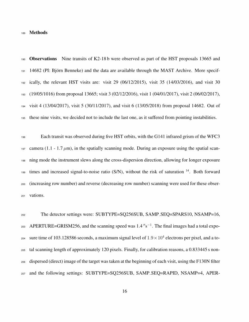
Methods189
Observations Nine transits of K2-18 b were observed as part of the HST proposals 13665 and190
14682 (PI: Bjorn Benneke) and the data are available through the MAST Archive. More specif-191
ically, the relevant HST visits are: visit 29 (06/12/2015), visit 35 (14/03/2016), and visit 30192
(19/05/1016) from proposal 13665; visit 3 (02/12/2016), visit 1 (04/01/2017), visit 2 (06/02/2017),193
visit 4 (13/04/2017), visit 5 (30/11/2017), and visit 6 (13/05/2018) from proposal 14682. Out of194
these nine visits, we decided not to include the last one, as it suffered from pointing instabilities.195
Each transit was observed during five HST orbits, with the G141 infrared grism of the WFC3196
camera (1.1 - 1.7µm), in the spatially scanning mode. During an exposure using the spatial scan-197
ning mode the instrument slews along the cross-dispersion direction, allowing for longer exposure198
times and increased signal-to-noise ratio (S/N), without the risk of saturation 14. Both forward199
(increasing row number) and reverse (decreasing row number) scanning were used for these obser-200
vations.201
The detector settings were: SUBTYPE=SQ256SUB, SAMP SEQ=SPARS10, NSAMP=16,202
APERTURE=GRISM256, and the scanning speed was 1.4 ′′s−1. The final images had a total expo-203
sure time of 103.128586 seconds, a maximum signal level of 1.9×10⁴ electrons per pixel, and a to-204
tal scanning length of approximately 120 pixels. Finally, for calibration reasons, a 0.833445 s non-205
dispersed (direct) image of the target was taken at the beginning of each visit, using the F130N filter206
and the following settings: SUBTYPE=SQ256SUB, SAMP SEQ=RAPID, NSAMP=4, APER-207
16

TURE=IRSUB256.208
Extracting the planetary spectrum We carried out the analysis of the eight K2-18 b tran-209
sits using our specialised software for the analysis of WFC3, spatially scanned spectroscopic210
images5, 17, 25, which has been integrated into the Iraclis package (see Code Availability section).211
The reduction process included the following steps: zero-read subtraction, reference pixels correc-212
tion, nonlinearity correction, dark current subtraction, gain conversion, sky background subtrac-213
tion, calibration, flat-field correction, and bad pixels/cosmic rays correction.214
We extracted the white (1.088 – 1.68µm) and the spectral (Supplementary Table 1) light215
curves from the reduced images, taking into account the geometric distortions caused by the tilted216
detector of the WFC3/IR channel25. The wavelength range of the white light curve corresponds to217
the edges of the WFC3/G141 throughput (where the throughput drops to 30% of the maximum).218
In addition, we tested two wavelength grids for the spectral light curves, with a resolving power of219
20 and 50. We decided to use the latter as it was able to capture the observed water feature more220
precisely – i.e there were enough data points within the wavelength range of the water feature to221
produce a statistically significant result.222
We fitted the light curves using our transit model package PyLightcurve, the transit param-223
eters shown in Supplementary Table 2, and limb-darkening coefficients (Supplementary Table 1)224
calculated based on the PHOENIX 31 model, the nonlinear formula32, and the stellar parameters in225
Supplementary Table 2.226
17

More specifically, we fitted the white light curves with a transit model (with the planet-to-star227
radius ratio and the mid-transit time being the only free parameters) alongside with a model for the228
systematics15, 25. It is common for WFC3 exoplanets observations to be affected by two kinds of229
time-dependent systematics33–36: the long-term and short-term “ramps”. The first affects each HST230
visit and has a linear behaviour, while the second affects each HST orbit and has an exponential231
behaviour. The formula we used for the systematics was the following:232
Rw(t) = nscanw (1− ra(t− T0))(1− rb1e
−rb2(t−to)) (1)
where t is time, nscanw is a normalisation factor, T0 is the mid-transit time, to is the time when each233
HST orbit starts, ra is the slope of a linear systematic trend along each HST visit and (rb1, rb2) are234
the coefficients of an exponential systematic trend along each HST orbit. The normalisation factor235
we used was changing to nforw for upwards scanning directions (forward scanning) and to nrev
w for236
downwards scanning directions (reverse scanning). The reason for using different normalisation237
factors is the slightly different effective exposure time due to the known up-stream/down-stream238
effect37. We, also, varied the parameters of the orbit-long exponential ramp for the first orbit in the239
analysed time-series (forb1, forb2 instead of rb1, rb2), as in many other HST observations the first240
orbit was affected in a different way compared to the other orbits5. While we used different ramp241
parameters from visit to visit, they appear to be consistent, an expected behaviour as the number242
of electrons collected per pixel per second is also consistent.243
At a first stage we fitted the white light curves using the formulas above and the uncertainties244
per pixel, as propagated through the data reduction process. However, it is common in HST/WFC3245
18

data to have additional scatter that cannot be explained by the ramp model. For this reason, we246
scaled-up the uncertainties on the individual data points, in order for their median to match the247
standard deviation of the residuals, and repeated the fitting5. From this second step of analysis,248
we found that the measured mid-transit times were not consistent with the expected ephemeris19,249
which we found to be: P = 32.94007±0.00003 days and T0 = 2457363.2109±0.0004 BJDTDB26.250
Supplementary Figure 1, shows the difference between the predicted and the observed transit times251
using the ephemeris in the literature19 and the one calculated in this work. We used the de-trended252
and time-aligned – i.e. with TTVs removed – white light curves to also refine the orbital parameters253
(a/R∗ = 81.3 ± 1.5 and i = 89.56 ± 0.02 deg). At a final step, we used all the new parameters254
(ephemeris, and orbital parameters) to perform a final fit on the white light curves (again having255
the planet-to-star radius ratio and the mid-transit time being the only free parameters).256
Supplementary Figure 2 shows the raw white light curves, the detrended white light curves257
and the fitting residuals as well as a number of diagnostics, while Supplementary Table 3 presents258
the fitting results. From these, we can see that:259
• the final planet-to-star radius ratio is consistent among the eight different transits, demon-260
strating the stability of both the instrument and the analysis process,261
• on average, the white light curve residuals show an autocorrelation of 0.17, which is a low262
number relatively to the currently published observations of transiting exoplanets with HST5263
(up to 0.7), indicating a good fit,264
• uncorrected systematics are still present in the residuals which, on average, show a scatter265
19

two times larger that the expected photon noise, and266
• this extra noise component is taken into account by the increased uncertainties, as the re-267
duced χ2 is, on average, 1.16.268
Furthermore, we fitted the spectral light curves with a transit model (with the planet-to-star269
radius ratio being the only free parameter) alongside with a model for the systematics that included270
the white light curve (divide-white method15), and a wavelength-dependent, visit-long slope25:271
Rλ(t) = nscanλ (1− χλ(t− T0))
LCw
Mw
(2)
where χλ is the slope of a wavelength-dependent linear systematic trend along each HST visit,272
LCw is the white light curve and Mw is the best-fit model for the white light curve. Again, the nor-273
malisation factor we used was changed to nforλ for upwards scanning directions (forward scanning)274
and to nrevλ for downwards scanning directions (reverse scanning). Also, in the same way as for275
the white light curves, we performed an initial fit using the pipeline uncertainties and then refitted276
while scaling these uncertainties up, in order for their median to match the standard deviation of277
the residuals.278
Supplementary Figures 3 to 19 show the raw spectral light curves, the detrended spectral light279
curves and the fitting residuals as well as a number of diagnostics, while Supplementary Table 4280
presents all the fitting results and average diagnostics per spectral channel. From these, we can see281
that:282
20

• the spectral light curves residuals show, on average, standard deviations much closer to the283
photon noise and lower values of autocorrelation, proving the advantage of using the white284
light curve as a model compared to the ramp model, and285
• any extra noise component is taken into account by the scaled-up uncertainties, as the re-286
duced χ2 is for all channels, on average, close to unity.287
Finally, the eight spectra of K2-18 b (Supplementary Figure 20) were combined, using a288
weighted average, to produce the final spectrum (Table 1).289
Stellar contamination K2-18 is a moderately active M2.5V star, with a variability of 1.7% in290
the B band and 1.38% in the R band40. Hence, to make sure that the observed water feature is291
not the effect of stellar contamination we fitted the observed spectrum with a model that assumes292
a flat planetary spectrum and contribution only from the star (M2V star as described in Rackham293
et al. 201841). The model that best describes our data has a spot coverage of 26% and a faculae294
coverage of 73%. We plot this spectrum versus the observed one in Supplementary Figure 21. In295
addition, we plot the spectrum produced by the spot and faculae combination reported by Rackham296
et al. 201841 and correspond to a 1% I-band variability, for reference. However, as Supplementary297
Figure 21 shows, the best-fit model cannot describe the observed water feature. From these we298
conclude that there is no combination of stellar properties that could introduce the observed water299
feature.300
21
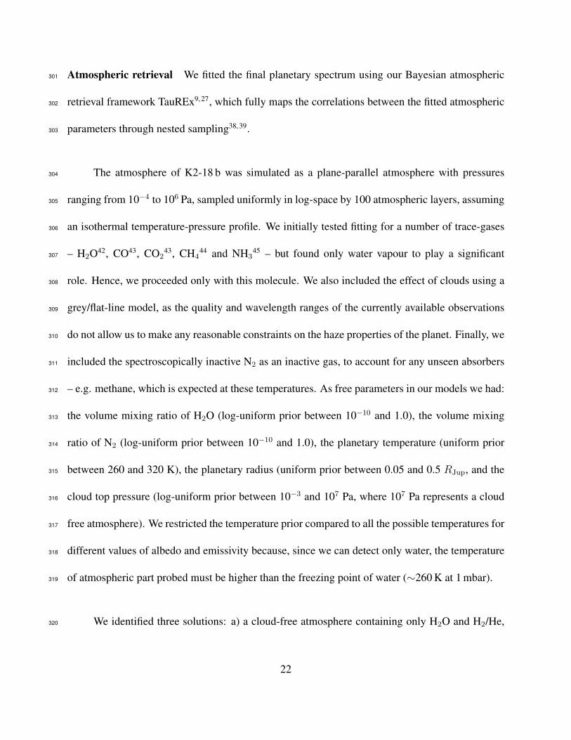
Atmospheric retrieval We fitted the final planetary spectrum using our Bayesian atmospheric301
retrieval framework TauREx9, 27, which fully maps the correlations between the fitted atmospheric302
parameters through nested sampling38, 39.303
The atmosphere of K2-18 b was simulated as a plane-parallel atmosphere with pressures304
ranging from 10−4 to 106 Pa, sampled uniformly in log-space by 100 atmospheric layers, assuming305
an isothermal temperature-pressure profile. We initially tested fitting for a number of trace-gases306
– H2O42, CO43, CO243, CH4
44 and NH345 – but found only water vapour to play a significant307
role. Hence, we proceeded only with this molecule. We also included the effect of clouds using a308
grey/flat-line model, as the quality and wavelength ranges of the currently available observations309
do not allow us to make any reasonable constraints on the haze properties of the planet. Finally, we310
included the spectroscopically inactive N2 as an inactive gas, to account for any unseen absorbers311
– e.g. methane, which is expected at these temperatures. As free parameters in our models we had:312
the volume mixing ratio of H2O (log-uniform prior between 10−10 and 1.0), the volume mixing313
ratio of N2 (log-uniform prior between 10−10 and 1.0), the planetary temperature (uniform prior314
between 260 and 320 K), the planetary radius (uniform prior between 0.05 and 0.5 RJup, and the315
cloud top pressure (log-uniform prior between 10−3 and 107 Pa, where 107 Pa represents a cloud316
free atmosphere). We restricted the temperature prior compared to all the possible temperatures for317
different values of albedo and emissivity because, since we can detect only water, the temperature318
of atmospheric part probed must be higher than the freezing point of water (∼260 K at 1 mbar).319
We identified three solutions: a) a cloud-free atmosphere containing only H2O and H2/He,320
22

b) a cloud-free atmosphere containing H2O, H2/He and N2, and c) a cloudy atmosphere containing321
only H2O and H2/He. The best-fit spectra and the posterior plots are shown in Figure 3. In all322
cases, a statistically significant atmosphere around K2-18 b was retrieved with an ADI5 of 5.0, 4.7323
and 4.0, respectively. The ADI is the positively defined logarithmic Bayes Factor, where the null324
hypothesis is a model that contains no active trace gases, Rayleigh scattering or collision induced325
absorption – i.e. a flat spectrum. An ADI of 5 corresponds to approximately a 3.6σ8, 9 detection of326
an atmosphere. The values are too similar to distinguish between the three scenarios.327
Data Availability The data analysed in this work are available through the NASA MAST HST328
archive (https://archive.stsci.edu) programs 13665 and 14682. The molecular line lists used are329
available from the ExoMol webpage (www.exomol.com). The final and intermediate results (re-330
duced data, extracted light curves, light curve fitting results and atmospheric fitting results) are331
available through the UCL-Exoplanets webpage (https://www.ucl.ac.uk/exoplanets).332
Code Availability All the software used to produced the presented results are publicly available333
through the UCL-Exoplanets GitHub page (https://github.com/ucl-exoplanets). More specifically,334
the codes used were:335
• TauREx (https://github.com/ucl-exoplanets/TauREx public),336
• Iraclis (https://github.com/ucl-exoplanets/Iraclis), and337
• PyLightcurve (https://github.com/ucl-exoplanets/pylightcurve).338
339
23

31. Allard, F., Homeier, D. & Freytag, B. Models of very-low-mass stars, brown dwarfs and340
exoplanets. Philos. Trans. Royal Soc. A 370, 2765–2777 (2012).341
32. Claret, A. A new non-linear limb-darkening law for LTE stellar atmosphere models. Calcula-342
tions for -5.0 <= log[M/H] <= +1, 2000 K <= Teff <= 50000 K at several surface gravities.343
Astron. Astrophys. 363, 1081–1190 (2000).344
33. Kreidberg, L. et al. A Detection of Water in the Transmission Spectrum of the Hot Jupiter345
WASP-12b and Implications for Its Atmospheric Composition. Astrophys. J. 814, 66 (2015).346
34. Evans, T. M. et al. Detection of H2O and Evidence for TiO/VO in an Ultra-hot Exoplanet347
Atmosphere. Astrophys. J. Lett. 822, L4 (2016).348
35. Line, M. R. et al. No Thermal Inversion and a Solar Water Abundance for the Hot Jupiter HD349
209458b from HST/WFC3 Spectroscopy. Astron. J. 152, 203 (2016).350
36. Wakeford, H. R. et al. HST PanCET program: A Cloudy Atmosphere for the Promising JWST351
Target WASP-101b. Astrophys. J. Lett. 835, L12 (2017).352
37. McCullough, P. & MacKenty, J. Considerations for using Spatial Scans with WFC3. Tech.353
Rep. (2012).354
38. Skilling, J. Nested sampling for general Bayesian computation. Bayesian Analysis 1, 833–860355
(2006).356
24

39. Feroz, F., Hobson, M. P. & Bridges, M. MULTINEST: an efficient and robust Bayesian in-357
ference tool for cosmology and particle physics. Mon. Not. R. Astron. Soc. 398, 1601–1614358
(2009).359
40. Sarkis, P. et al. The CARMENES Search for Exoplanets around M Dwarfs: A Low-mass360
Planet in the Temperate Zone of the Nearby K2-18. Astron. J. 155, 257 (2018).361
41. Rackham, B. V., Apai, D. & Giampapa, M. S. The Transit Light Source Effect: False Spec-362
tral Features and Incorrect Densities for M-dwarf Transiting Planets. Astrophys. J. 853, 122363
(2018).364
42. Barber, R. J., Tennyson, J., Harris, G. J. & Tolchenov, R. N. A high-accuracy computed water365
line list. Mon. Not. R. Astron. Soc. 368, 1087–1094 (2006).366
43. Rothman, L. S. et al. HITEMP, the high-temperature molecular spectroscopic database. J. of367
Quant. Spec. & Rad. Transf. 111, 2139–2150 (2010).368
44. Yurchenko, S. N. & Tennyson, J. ExoMol line lists - IV. The rotation-vibration spectrum of369
methane up to 1500 K. Mon. Not. R. Astron. Soc. 440, 1649–1661 (2014).370
45. Yurchenko, S. N., Barber, R. J. & Tennyson, J. A variationally computed line list for hot NH3.371
Mon. Not. R. Astron. Soc. 413, 1828–1834 (2011).372
46. Foreman-Mackey, D. corner.py: Scatterplot matrices in python. The Journal of Open Source373
Software 24 (2016).374
25
Top Related