


Languages
Pages
Legal

Wage Inequality in International Perspective:
Effects of Location, Sector, and Gender
Thomas Hertz, Paul Winters, Ana Paula de la O,
Esteban J. Quiñones, Benjamin Davis and Alberto Zezza
ESA Working Paper No. 08-08
November 2008
Agricultural Development Economics Division The Food and Agriculture Organization of the United Nations
www.fao.org/es/esa

ESA Working Paper No 08-08 www.fao.org/es/esa
Wage Inequality in International Perspective:
Effects of Location, Sector, and Gender
November 2008
Thomas Hertz
Agricultural Development Economics Division Food and Agriculture Organization
Rome, Italy e-mail: [email protected]
Paul Winters
American University Washington, DC
USA e-mail: [email protected]
Ana Paula de la O Agricultural Development Economics Division
Food and Agriculture Organization Rome, Italy
e-mail: [email protected]
Esteban J. Quiñones
The International Food Policy Research Institute (IFPRI
Washington D.C USA
e-mail: [email protected]
Benjamin Davis
Agricultural Development Economics Division Food and Agriculture Organization
Rome, Italy e-mail: [email protected]
Alberto Zezza
Agricultural Development Economics Division Food and Agriculture Organization
Rome, Italy e-mail: [email protected]
Abstract This paper uses the well-known Oaxaca-Blinder decomposition technique to understand the determinants of wage-gaps between men and women, between urban and rural workers, and between those employed in the rural agricultural versus the rural non-agricultural sectors, for the 14 developing and transition economies in the RIGA-L dataset. The unexplained male-female wage gaps (i.e. the gaps that remain after controlling for a host of observable characteristics of the job and the worker) provide estimates of labor market discrimination against women that are consistent with prior estimates from other countries, and are generally similar in rural and urban areas. We argue that countries with large unexplained urban-rural gaps, such Tajikistan and Malawi, are those in which rural to urban migration is likely to persist even in face of high urban unemployment rates. Furthermore, we find that large unexplained wage gaps in favor of non-farm employment, versus paid labor in farming, exist in Tajikistan (53%), Ecuador (44%), Nepal (36%), Nicaragua (32%), and Nigeria (30%); these would then appear to be the countries for which a shift of existing workers, with their current attributes, from the farm to the non-farm sector would have the largest impact on rural incomes. Key Words: Urban/rural wage differentials, agricultural wages, gender discrimination. JEL: J31, J71, R23, O18. The designations employed and the presentation of material in this information product do not imply the expression of any opinion whatsoever on the part of the Food and Agriculture Organization of the United Nations concerning the legal status of any country, territory, city or area or of its authorities, or concerning the delimitation of its frontiers or boundaries.
1
Wage inequality in international perspective:
Effects of location, sector, and gender
1. Introduction
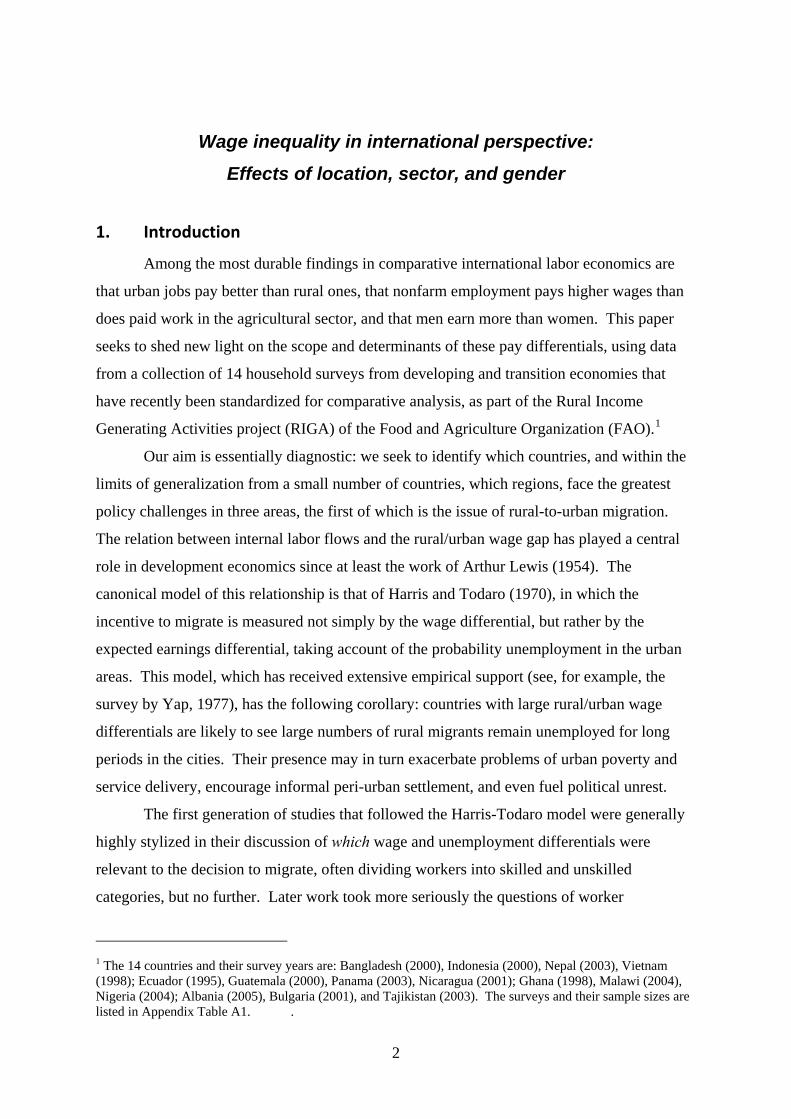
Among the most durable findings in comparative international labor economics are
that urban jobs pay better than rural ones, that nonfarm employment pays higher wages than
does paid work in the agricultural sector, and that men earn more than women. This paper
seeks to shed new light on the scope and determinants of these pay differentials, using data
from a collection of 14 household surveys from developing and transition economies that
have recently been standardized for comparative analysis, as part of the Rural Income
Generating Activities project (RIGA) of the Food and Agriculture Organization (FAO).1
Our aim is essentially diagnostic: we seek to identify which countries, and within the
limits of generalization from a small number of countries, which regions, face the greatest
policy challenges in three areas, the first of which is the issue of rural-to-urban migration.
The relation between internal labor flows and the rural/urban wage gap has played a central
role in development economics since at least the work of Arthur Lewis (1954). The
canonical model of this relationship is that of Harris and Todaro (1970), in which the
incentive to migrate is measured not simply by the wage differential, but rather by the
expected earnings differential, taking account of the probability unemployment in the urban
areas. This model, which has received extensive empirical support (see, for example, the
survey by Yap, 1977), has the following corollary: countries with large rural/urban wage
differentials are likely to see large numbers of rural migrants remain unemployed for long
periods in the cities. Their presence may in turn exacerbate problems of urban poverty and
service delivery, encourage informal peri-urban settlement, and even fuel political unrest.
The first generation of studies that followed the Harris-Todaro model were generally
highly stylized in their discussion of which wage and unemployment differentials were
relevant to the decision to migrate, often dividing workers into skilled and unskilled
categories, but no further. Later work took more seriously the questions of worker
1 The 14 countries and their survey years are: Bangladesh (2000), Indonesia (2000), Nepal (2003), Vietnam (1998); Ecuador (1995), Guatemala (2000), Panama (2003), Nicaragua (2001); Ghana (1998), Malawi (2004), Nigeria (2004); Albania (2005), Bulgaria (2001), and Tajikistan (2003). The surveys and their sample sizes are listed in Appendix Table A1. .
2

heterogeneity, of the econometric estimation of counterfactual earnings opportunities, of the
quality of rural workers’ information about urban wages and employment prospects, of
cyclical or return migration, and of the possibility that perceived income gaps might depend
on the migrant’s choice of reference group, and hence on relative versus absolute wage
comparisons (Stark and Bloom, 1985; Stark, 1995; Ghatak, Levine, and Price, 1996).
In this paper we take a middle-ground approach to the estimation of the relevant wage
differential between urban and rural areas, ignoring some of the more complex issues just
cited. We employ a straightforward technique that has long been a staple of the analysis of
race and gender-based wage differentials, namely, the Oaxaca-Blinder decomposition
(Oaxaca, 1973; Blinder, 1973). This adjusts the observed gap in mean wages between two
groups for differences in the average attributes (or “assets”) of each class of worker (often
including factors such as occupation and industry). The remaining, unexplained, portion of
the wage gap is then due to differences in the rates at which these assets are remunerated in
(say) rural versus urban labor markets (differences in “prices”). This adjustment, we argue,
approximates the effort made by the average rural worker to estimate the gain in wages that
“people like me” could expect to receive if they found employment in the city. The
decomposition technique is essentially no different than comparing like individuals in the two
locations, based on observed wages and observed characteristics.
As such, it may well be plagued by problems of sample selection bias, the solution of
which preoccupies much of the empirical literature (Stark, 1995). The problem is that the
comparison of wages for ostensibly similar individuals in the two areas may not yield a good
measure of the counterfactual wage that would be earned by the marginal migrant,
particularly if those with the highest levels of unobserved skills are the first to migrate, or the
first to be employed. Yet we argue that such complex arguments are likely to be of second-
order (or lower) importance to the migrants themselves, who must work with the information
they have, much of which will be anecdotal, i.e. derived from reports of wages earned by
people to whom they consider themselves similar, based on observable factors.
Our approach yields what might be called a standardized descriptive model of wage
differences: the results are not offered as unbiased estimates of structural (causal) parameters,
yet, because the technique of description and the set of conditioning variables are
standardized across countries, comparisons of results may yield valuable insight into the
3

proximate determinants of the relevant rural/urban wage gap in each country, at roughly the
same level of sophistication as might be employed by the migrants themselves.2
Our second comparison, between wages in agricultural versus nonfarm employment,
serves a similar purpose.3 While early models of development typically conflated the rural
with the agricultural as a matter of convenience,4 this simplification has become less
convenient as rural nonfarm employment has grown in importance (FAO, 1998; Reardon,
Berdegue, and Escobar, 2001; Davis, et al., 2007). Moreover, the fact that nonfarm jobs
generally pay higher wages that do farm jobs suggests that rural economic development may
hinge on the movement of wage labor from the farm sector to other rural economic activities,
if not to the cities. Using the same data we will employ, Winters et al. (2008), show that
while agricultural jobs generally do pay less, there is still a considerable overlap between the
farm and nonfarm wage distributions in most countries. They argue that the sector of
employment is a less important determinant of access to high-productivity jobs than are
factors such as education and the quality of local infrastructure. Still, it remains important to
determine just how large the wage advantage is, or appears to be, for a worker who moves
from a farm job to a nonfarm job, given current levels of education and infrastructure, and
this is what our method is well-suited to measure. Countries that display large unexplained
pay differentials between agricultural and non-agricultural work are likely to be those in
which the exodus of wage labor out of agriculture will be most rapid, and for which this shift
in employment patterns represents a viable way of raising rural incomes, particularly if
2 Although the Oaxaca-Blinder decomposition is predominantly employed in the study of race and gender discrimination, we are not the first to apply it to the study of the urban-rural divide. For example, Sicular, et al. (2007) use the method to show that rural location per se is the most important source of rural-urban income gaps in China, followed by education, while factors such as family size, landholdings, and Communist party membership are relatively unimportant. Unexplained rural-urban wage gaps are also documented for Brazil (Loureiro and Carneiro, 2001), while Gabe, Colby, and Bell (2007, p. 1) use the Oaxaca method to demonstrate that: “Differences in the proportions of creative workers [which they identify with ‘technology-based segments of the super-creative core such as computer and mathematical, architecture and engineering, and scientific occupations’] between metropolitan and non-metropolitan counties contribute 11.5 percent to the U.S. rural-urban wage gap.” The study most similar to our own is perhaps that of Agesa and Agesa (1999), who use the Oaxaca approach to estimate the incentives to migrate in Kenya. However, they find it important to control for selection bias due to differences in both migration and employment probabilities, which we argue is not needed. This is not to say that such adjustments are not needed in other contexts: for example, if one wishes to estimate differences in wage offers as opposed to observed wages, in order to measure race or gender discrimination, then Heckman-selection-corrected Oaxaca decompositions, such as implemented by Reimers (1983), for example, are appropriate in principle, if often difficult to implement in empirically convincing fashion, as discussed below. 3 Note that this analysis excludes rural own-account farming, for reasons explained below. 4 As an example, consider the work of Lewis, already cited, or that of Lipton, who, in arguing for his urban bias hypothesis, used the ratio of income per person in the non-agricultural and agricultural sectors as his basic measure of the rural/urban disparity, while noting that this might slightly overstate the gap (1977; 1984, p. 140).
4

nonfarm investment responds in some proportion to the size of the wage differential, i.e.
seeks to exploit the fact that additional workers may be attracted to the nonfarm sector at
lower wages than are currently being paid. By contrast, we will demonstrate that for some
countries this pay differential is negative, meaning that no such incentives exist on either the
supply or the demand side of the nonfarm labor market.
Our third outcome, the male-female wage differential, is, of course, a fundamental
measure of gender equality. Grimshaw and Rubery (2002) note that gender wage gaps have
now been included among the structural criteria by which the European Commission will
judge economic equity, but that to make this judgment requires that one take account of the
different skills and levels of experience that men and women may bring to the labor market,
which is exactly what the Oaxaca decomposition seeks to do. In this application, the
unexplained wage gap, or the portion due to differences in “prices,” is often identified with
discrimination, although, as we will see, it is at best an imperfect measure of employer
discrimination in the labor market. Here the policy implications have nothing to do with the
incentive to move from one group to the other; instead comparing the results across various
countries, using comparable specifications and comparably structured datasets, should allow
us to draw some general conclusions about their relative degrees of gender bias, and about
which policy interventions might be most effective in reducing gender disparities.
In analyzing the male/female wage gap we first stratify the data for each country into
its urban and rural areas, in order to test the proposition that gender pay gaps might be
affected by institutional differences between the two. On average, we find no clear cut
rural/urban difference in either the size of the wage gap, or the share of it that can be
explained by differences in assets. In both the cities and the countryside, men earn about 25
percent more than women5, on average across our sample, and only two or three of these
percentage points can be attributed to asset differences, by which we mean human capital or
demographic differences (age, education, ethnicity, marital status, number of children);
additional characteristics which describe both the job, and, indirectly, the skills of the job-
5 All of our wage data are in natural logarithms, and when we speak of percentage differences we are actually referring to log point differences. Differences of 40 log points or less are reasonably close approximations of standard arithmetic percentage differences: a 40 log point gap between men and women implies that the geometric mean wage for men is 49 percent higher than for women, or that women earn 33 percent less than men. The advantage of the log point construction is that it splits the difference between these two values, eliminating the need to specify in which direction the percentage change was calculated. At higher values, however, the approximation can be misleading, and we will refer to these larger values as “log point differences” to remind the reader of this fact.
5

holder (public or private sector, main or secondary job, full or part-time status, occupation,
industry); and a set of controls for region and the quality of local infrastructure.
The RIGA data also allow us to add eight new countries6 to the list of those for which
gender wage gaps may be analyzed by this method, and to provide updated results for six
more.7 Combining our data with other published results generates a dataset of 121 country-
years for which the male-female wage gap can be studied in this way. For this group we
demonstrate that the unexplained male wage advantage bears no relationship at all to the level
of development (as measured by PPP income per capita in constant dollars). Further analysis
of this question is the subject of work in progress.
Together, these three analyses summarize the relative magnitudes of three important
dimensions of interpersonal inequality in developing and transition economies, namely, those
due to location, sector, and gender, and provide rough estimates of the degree to which these
inequalities might be reduced through the manipulation of either asset endowments (e.g.
educational interventions, or rural road building) or prices (e.g. antidiscrimination policies).
Because our sample of countries for which rural/urban and farm/nonfarm wage gaps can be
studied is too small to support a cross country regression analysis, for these two outcomes we
will limit ourselves to identifying those countries that fall at the high and low ends of the
spectrum of unexplained inequality, the policy implications of which we have described.
2. Data
The RIGA dataset builds on surveys drawn primarily from the World Bank’s
collection of Living Standards Measurement Surveys.8 Some 25 such surveys have been
standardized to facilitate comparative cross-country analysis at the household level, and have
been used such purposes as the study of the role of access to agricultural assets and
institutions in determining farming outcomes (Zezza, et al., 2008b) and the estimation of the
impact on poverty of the recent spike in food prices (Zezza, et al., 2008a). This paper draws
on a subset of 14 of these datasets for which the individual-level labor market data have been
rigorously cleaned and coded for comparability, as described by Quiñones, et al. (2008). All 6 Our review of the literature found no prior Oaxaca estimates for Albania, Bangladesh, Ghana, Malawi, Nepal, Nigeria, Tajikistan, or Vietnam. 7 The updated countries are Bulgaria (2001), Ecuador (1995), Guatemala (2000), Indonesia (2000), Nicaragua (2001), and Panama (2003). 8 Two of the surveys incorporated in this analysis are not from the LSMS collection: these are for Indonesia (undertaken by the Rand Corporation) and Bangladesh (undertaken by the Bangladesh Bureau of Statistics).
6

analyses are conducted at the level of the job, not the person, since most surveys allow people
to report more than one job held in the last year. Our sample consists of all recorded jobs
held by those between the ages of 15 and 65, and includes casual, part-time, and temporary or
seasonal employment as well as regular full-time jobs. Note however that our data on farm
employment do not reflect agricultural self-employment, despite its importance as a source of
rural income. This is because the implicit wages associated with family farming are
extremely difficult to estimate at the individual level without more detailed data on time use
than is generally available.
Wages are analyzed in terms of local currency units per day, rather than per hour,
because hours of work were not always reliably available. In discussing our conclusions we
check them against the findings that emerge for the subset of nine of our 14 countries for
which hourly wages were calculable.
3. Methods
The Oaxaca-Blinder decomposition technique was developed independently by these
two economists in 1973, and has since been elaborated on by Cotton (1988) and Neumark
(1988) among others. Its virtue lies in allowing for the possibility that discrimination might
be reflected not just in a fixed differential between the wages of, for example, men versus
women, but also by differences in the rewards associated with increases in men’s versus
women’s human capital. The wisdom of this observation has recently been affirmed in an
analysis of hiring (as opposed to wage) discrimination against African-Americans, which
found that educational credentials are heavily discounted for blacks, and that this explains a
portion of their lower interview call-back rate by employers who, in a randomized
experiment, were sent fabricated resumes that differed only in the “whiteness” of the
applicants’ names (Mullainathan and Bertrand, 2004).
To implement the decomposition one runs separate regression equations, by group, of
log wages (W) against a chosen set of predictors (X). These yield parameter estimates β1 for
group 1 and β2 for group 2. Note that these parameters include the intercepts for each
equation, and thus subsume the group indicator variable that one would otherwise employ in
a pooled analysis. The difference in mean log wages can then be written:
7

[1] ∑∑ −+−=−j
jjjj
jjj XXXWW )()( 21221121 βββ
where j ranges over the elements of X. The first term sums the portion of the wage
differential that can be attributed to differences between the groups in their values of X, while
the second term captures the contribution of differences in the economic rewards to these
attributes.
Both Neumark (1988) and Cotton (1988) note that the choice of the first group’s
parameter vector as the one by which differences due to attributes (first term) are evaluated is
arbitrary. They argue that the relevant parameter vector is the hypothetical one that would
obtain in a non-discriminatory environment, although they differ in how to estimate that. We
follow Cotton in using the simple weighted average of the group-specific parameter vectors
as our reference point. Our choice does not rest on an explicit model of labor market
discrimination, but simply represents a plausible and transparent way to split the difference
between the two choices of reference group. We thus decompose the wage differential as
follows:
[2] ⎪⎭
⎪⎬⎫
⎪⎩
⎪⎨⎧
−−−+−=− ∑∑∑j
jjjj
jjjj
jjj XXXXWW )()()( 22112121 βββββ
where 21 )1( jjj βααββ −+= , and α is just group 1’s share in the sample.
The first summation represents the explainable portion of the wage gap: it measures
the effects of group differences in assets, evaluated using a price vector that is intermediate
between the two group-specific sets of prices. The term in set brackets captures the portion
of the wage gap that is due to deviations of each group’s price vector from the average,
evaluated at each group’s mean asset values. In other words, it captures group differences in
the rate of return to each asset, including group membership itself (the intercept).
The results of such an exercise depend critically on the choice of variables for X.
We first include a set of controls for human capital and demographics, namely, age,
education, membership in the dominant ethnic or religious group, and marital status, as well
as a proxy measure for the number of children each woman may have had to care for.9 This
last variable is included in an attempt to address the problem of the mismeasurement of
women’s work experience, due to time spent outside the paid workforce raising children. It
9 The number of children a woman has actually borne and raised is not generally known in these surveys. As a proxy, we counted the number of household members in the generations younger than the woman in question.
8

is set to zero for all men, on the assumption that men do not lose work experience in
proportion to the number of children they have. In the regressions for the rural/urban and
farm/nonfarm gap, we also include a gender dummy variable.
Next come a set of controls for public sector employment, main or secondary jobs,
part-time status, occupation, and industry (the latter being omitted in the agriculture
equations). The number of occupational controls was generally on the order of five
categories, while the number of industries was usually ten; these are consistent with many
other analyses of the gender wage gap (Grimshaw and Rubery, 2002). Last, we include
region dummies (their number being determined by each survey’s definition of regional
boundaries) and an infrastructure index which measures the distance from the household to
schools, medical facilities, roads, communication services, and other related services. This
serves as a measure of the difficulty of access to local labor markets, and to public services
that help build and sustain human capital (see Winters et al. (2008) for details of its
construction).10
In the male/female comparison, the term in set brackets in equation 2 is often
identified with the extent of gender discrimination in the labor market, but it may either over
or understate the extent of this problem, depending on which covariates are included in the X
matrix. An overstatement of discrimination could arise if one cannot fully measure all
dimensions of human capital, such as experience, job-specific skills, or any of a number of
“soft skills” or personality traits that have been shown to be important in many occupations.
As already noted, women’s work experience is often poorly measured because most surveys
do not undertake a full lifetime accounting of time in and out of the labor market.
On the other hand, societal discrimination against women can easily be understated
by this method. In particular, the inclusion of occupational control variables will cause us to
miss the possible effects of involuntary or custom-driven occupational segregation; thus, by
including the occupational controls we err on the side of understating labor market
discrimination against women. Yet to exclude occupational controls is also problematic, to
the extent that group wages differ because of freely-determined choices of occupation. The
same goes for such crucial variables as the level of schooling: to exclude it is obviously
problematic, yet to include it is to ignore the effects of discrimination in the provision of
education, or in the setting of girls’ aspirations. While these are arguably not problems in the
10 The infrastructure index is omitted from the urban-rural comparison, and from the male-female comparison in urban areas, as it is only defined for rural households.
9

labor market per se, they are clearly of interest in assessing women’s economic status.
Finally, sample selection bias may prevent our estimates of the determinants of
observed wages from coinciding with the true determinants of wages offered to men versus
women, and this matters for understanding discrimination. Many race and gender analyses
attempt to correct for selection bias using Heckman’s (1979) approach. However, as many
have noted, Heckman’s model depends strongly on the assumptions of homoskedasticity and
normality, and on the validity of omitting the participation-predicting variables (instruments)
from the wage equation. Deaton (1997) argues that the canonical example, that of Gronau
(1974), in which the number of children a woman has is used to predict her labor market
participation, is a successful application of the technique, but that such successes may be the
exception rather than the rule. Indeed, even in this case the validity of the model can be
challenged: if work experience is poorly measured, and is reduced by time spent raising
children, then the number of children belongs in the wage equation as a proxy for lost
experience, in which case it cannot serve to identify the participation propensity. Moreover,
when Heckman’s model is used with no additional instruments, the identification of selection
bias rests entirely on the choice of functional form, which is not an adequate foundation, and
may easily lead to results that are more biased than the uncorrected ones.
Given these problems, we do not attempt selection-corrections for our gender results,
although we readily admit they should matter in principle in this case. Nor, given the
problems of defining the optimal set of control variables, do we claim that the unexplained
wage gap (due to prices, or coefficients) is a pure measure of wage discrimination per se.
Still, we consider the unexplained gaps to be useful if imperfect summary measures of gender
bias, more useful in cross-country comparison than in isolation. Similarly, the unexplained
rural/urban and farm/nonfarm wage gaps are offered as summary measures of the market
imperfections that allow wages to differ across space and economic sector, and which thereby
create incentives for labor mobility.
The nature of the explained portion of each wage gap also has policy implications. In
the realm of education, for example, they tell us how much of the observed wage differential
can be attributed to differences in the levels of schooling held by members of each group: if
these schooling gaps are large and consequential then the usual array of policies to encourage
educational attainment for the disadvantaged group are called for. As we shall see, on
average for our 14 countries, educational gaps explain virtually none of the difference
between men’s and women’s mean log wages, implying that the “more schooling”
prescription is not likely to be effective in reducing gender pay disparities. Differences in the
10
level of education play a somewhat larger role in explaining the rural/urban and
farm/nonfarm wage gaps, but not as much as one might expect.
By contrast, if the rewards to education differ across groups, the interpretation is
somewhat more tricky: on the one hand, differential rewards may reflect discriminatory
behavior on the part of employers (as when women’s educational qualifications are not
rewarded at the same rate as men’s); or they may reflect technology-driven differences in the
relation between education and productivity (as in farm versus nonfarm labor); or they may
reflect unmeasured differences in the quality of education (as in urban versus rural areas).
This latter example serves to remind us, again, that observed urban wages may not in fact be
the proper counterfactual wage that a migrant could expect to receive. Still, it is plausible to
argue that a migrant with a high school education, when looking at the wages of urban high
school graduates in making her migration decision, would probably not mentally adjust these
for differences in the quality of education between rural and urban schools.
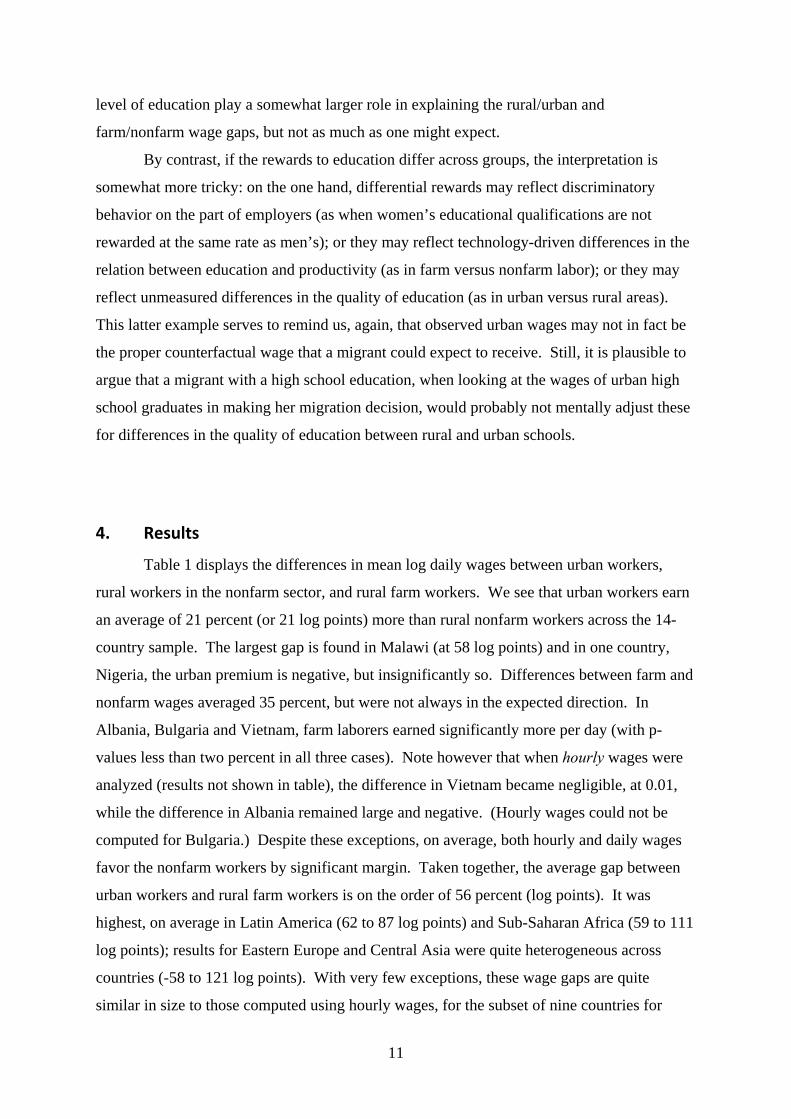
4. Results
Table 1 displays the differences in mean log daily wages between urban workers,
rural workers in the nonfarm sector, and rural farm workers. We see that urban workers earn
an average of 21 percent (or 21 log points) more than rural nonfarm workers across the 14-
country sample. The largest gap is found in Malawi (at 58 log points) and in one country,
Nigeria, the urban premium is negative, but insignificantly so. Differences between farm and
nonfarm wages averaged 35 percent, but were not always in the expected direction. In
Albania, Bulgaria and Vietnam, farm laborers earned significantly more per day (with p-
values less than two percent in all three cases). Note however that when hourly wages were
analyzed (results not shown in table), the difference in Vietnam became negligible, at 0.01,
while the difference in Albania remained large and negative. (Hourly wages could not be
computed for Bulgaria.) Despite these exceptions, on average, both hourly and daily wages
favor the nonfarm workers by significant margin. Taken together, the average gap between
urban workers and rural farm workers is on the order of 56 percent (log points). It was
highest, on average in Latin America (62 to 87 log points) and Sub-Saharan Africa (59 to 111
log points); results for Eastern Europe and Central Asia were quite heterogeneous across
countries (-58 to 121 log points). With very few exceptions, these wage gaps are quite
similar in size to those computed using hourly wages, for the subset of nine countries for
11

which the comparison is feasible (see Appendix, Table A2). All of the conclusions that
follow are qualitatively and quantitatively similar in the hourly wage data, unless otherwise
noted.
The urban/rural Oaxaca decomposition results (now counting farm and nonfarm jobs
together) are reported in Table 2. The raw wage gap averaged 41 percent in favor of the
urban areas; results for the four Latin American countries were similar, and on the higher end
of the spectrum (42 to 57 log points), while for Asia the gap was between 28 and 40 percent.
The other two regions were quite heterogeneous, with large numbers for Malawi (102) and
Tajikistan (96), and low numbers for Nigeria (16), Bulgaria (10), and Albania (-5).
On average across the 14 countries, 24 of the 41 percentage points that separate urban
and rural average wages could be attributed to differences in the assets or attributes listed
above (see column labeled “Total Due to Assets.”) Not surprisingly, urban/rural education
differences loomed as the largest single explanatory factor (accounting for 9 percentage
points), with differences in occupation (6 points) and industry (5) following close behind.
Taken together these three factors thus explain 20 of the 24 percentage points we were able to
attribute to asset differences for the sample as a whole.
The next panel shows that, on average, 17 percentage points of the wage gap were
attributed to urban/rural differences in “prices,” or the estimated regression coefficients from
the wage equations (see column labeled “Total Due to Prices.”) This “unexplained” gap was
highest in Tajikistan (46 points) and Malawi (49 points). As argued above, this implies that
the incentives for rural-to-urban migration should be quite strong in these two countries, and
that migrants would tolerate considerable levels of urban unemployment. A crucial caveat,
however, is that our wage rates are not adjusted for local differences in the cost of living; but
neither are they adjusted for hedonic differences in the quality of life in urban versus rural
areas.
Four countries stand out as having exceptionally low unexplained urban/rural wage
gaps: these are Guatemala (2 percent), Albania (4 percent), Nepal (4 percent), and Nicaragua
(7 percent). Note that in three of these cases (all but Albania) the raw (unadjusted)
urban/rural wage gap is not especially low, ranging between 28 and 51 points. Instead, the
small unexplained gap arises because we are able to explain away most of the observed wage
gap. The final column echoes this fact: it reports the percentage share of the wage gap that
remains unexplained, which is low for these three countries (between 4 and 17 percent of the
12

total) compared to the sample as a whole (40 percent share unexplained)11. In other words,
asset differences are the primary reason for the urban/rural wage gap in these three countries.
If migrants perceive this fact correctly, then they should not expect large wage increases were
they to obtain an urban job, and hence may be less likely to end up unemployed in the urban
areas. In Albania, both the raw and the unexplained wage gaps are low, or negative, which
likewise suggests that rural dwellers have little if any incentive to migrate.
Differences in the returns to education, evaluated at each group’s mean level of
schooling, do not systematically favor one group over the other, although they do make a
large negative contribution to the wage gap (i.e. they favor rural workers) in Albania and
Bulgaria, and a large positive contribution in Tajikistan (see column titled “Educ” under the
heading “Due to Price Differences (“Unexplained”)). By contrast, differences in the returns
to age favor urban workers in all but two cases, and, on average, generate a 28 percent wage
advantage for city-dwellers, with especially high results for Sub-Saharan Africa.12 Figure 1
illustrates the case of Vietnam, which is representative of the sample average. To interpret
this graph, recall that these predicted (log) wages are based solely on the effects of age – they
do not represent the gap in pay between the average urban or rural worker, but only the way
that gap evolves with age, all else being equal. We see that urban workers experience faster
wage growth, such that by about age 30 they are 28 percent ahead of rural workers, by virtue
of greater returns to age alone. This may occur for various reasons: pay for urban jobs may
be more often governed by conventions that reward job tenure and experience; opportunities
to advance from lower to higher paying occupations (within our fairly broad occupational
categories) may be greater in the cities than in the countryside; and experience may actually
have a more direct effect on productivity in the urban than in the rural sector. But it is also a
finding that emerges in relation to the other group differences we study, and, indeed, in many
other contexts: higher paid groups generally display steeper age-wage profiles.
Table 3 presents the result for the comparison of paid employment in the farm and
nonfarm sectors. The raw wage gap was 35 percent on average, and was again significantly
influenced by differences in education, and occupation, as well as public sector employment.
The latter makes sense, given that the public sector jobs often pay more in developing
11 The figure 0.40 represents the simple average of the unexplained shares for each country. Below it appears an alternative estimate. which weights countries with larger wage gaps more heavily. This is just equal to the average of the “Total Due to Prices” column divided by the average of the “Log Wage Gap” column. 12 Note that the contributions of differences in prices cannot be assessed for variables that are entered as sets of indicators, such as occupation, industry, and region. This is because the results depend on the arbitrary choice of the omitted reference category. However, the overall “unexplained” effect is invariant to these choices.
13
countries and are rarely agricultural (the formerly communist countries being the exception to
this rule). Infrastructure effects were generally positive, particularly in Panama, Indonesia,
and Sub-Saharan Africa, meaning that those in non-farm employment benefited from their
proximity to markets and services; this supports the conclusions of Winters et al. (2008) who
note the positive role of infrastructure development in stimulating higher paid employment.
Taken together, asset differences explain roughly half of the observed wage gap,
leaving the other half unexplained. Within this unexplained category, age-profile-effects
again loom very large: non-farm workers benefit from steeper age-wage profiles in 12 of the
14 countries. Surprisingly, there is no systematic effect of differences in the returns to
education, despite the fact that returns to education in agriculture are often presumed to be
low. This finding, however, requires careful interpretation: first, these regressions do not
estimate the full benefits, private or social, of education; and second, in the majority of
countries of the world, the returns to schooling are greatest at the lowest levels of schooling
(Psacharopoulos, 2006). Thus they may be higher for poorly educated farm workers than for
better educated nonfarm workers, even if the relation between education and productivity at
any given level of schooling is stronger in the non-farm sector.
Countries that displayed an unexplained rural non-agricultural wage premium of more
than 30 percent included Tajikistan (53), Ecuador (44), Nepal (36), Nicaragua (32), Nigeria
(30); these would then appear to be the countries for which a shift of existing workers, with
their current attributes, from the farm to the non-farm sector would have the largest impact.
As before, the formerly communist countries of Albania and Bulgaria are the exceptions in
the other direction: rural wages are higher in the paid farm sector, both in raw and adjusted
terms.
Tables 4 and 5 report the results of the decompositions by gender for rural and for
urban areas. The average gender gap in daily wages across the 14 countries was on the order
of 25 percent in favor of men, in both the cities and the countryside. In just one case, rural
Panama, were observed wages higher for women than men (by 11 percent) while in countries
such as Indonesia, Ecuador, Ghana, Albania and Tajikistan the male-female gap was as large
as 38 to 60 log points. There was no clear regional pattern to the size of the raw wage
difference, yet there is a clear regional difference in the breakdown between its explained and
unexplained components. In most countries outside of Latin America, at least some portion
of the male wage advantage can be explained by their education, age, industry, and so forth.
In Latin America, by contrast, women’s attributes are superior to men’s in all comparisons
except rural Ecuador: if these attributes were rewarded equally, women would earn more than
14

men, but in fact they earn less, a situation which may be termed “hyper discrimination” and
which is reflected by an unexplained share that exceeds 100 percent.
Driven in part by these extreme figures for Latin America, the average unexplained
share of the wage gap was also very high, at roughly 90 percent, for both rural and urban
areas, meaning that our cross-country average estimate of gender bias is about 22 percent.
And while assets have virtually no explanatory power, on average, differences in the returns
to age again appear significant, at least in the rural areas: they favor men in 10 of the 14
countries, whereas in urban areas they favor men by a smaller margin and in fewer countries.
Part of the reason for the gender difference in age profiles may be that women who raise
children typically accumulate fewer years of labor market experience per year of age, unless
policies (or spouses) are in place that permit women with young children to maintain their
employment status. Although we do control for the estimated number of children, this
control is imperfect, and unmeasured differences in work experience doubtless remain.
Figure 2 illustrates the age effect for rural Nepal, where the gap between male and female
wages due to their differing age profiles was near the rural sample average, at 18 percent.
Note that women’s wages peak at age 38, while men’s rise until age 56, holding all other
factors equal.
Figure 3 illustrates the relation, or lack thereof, between the unexplained wage gap
and the level of development, as measured by purchasing power parity estimates of per capita
real income, in 67 different countries observed between 1980 and 2005, for a total of 121
observations.13 For comparability with other published results we chose to use only the
urban RIGA data, and, where possible, to base the estimates on hourly wages rather than
wages. The scatter plot reveals a wide range of estimates of gender bias (with just two cases
of “reverse discrimination”) but no relation whatsoever to the level of income: the average
unexplained male premium is around 25 percent at all levels of development, consistent with
the results from our 14 countries.
day
This finding also holds true when one includes controls for the year of the survey,
whether as dummies for each year or as a linear time trend. In the latter case, however, the
time trend is significant (p=0.05, based on robust standard errors, clustered on country),
implying that gender wage bias is falling at a rate of about 4 percentage points per decade, as
illustrated in Figure 4. However, it is important to note that all of the most recent estimates
13 The list of studies used in this estimation are available from the authors upon request, and will be documented in forthcoming work, now in progress.
15
come from our own analysis, and that without these additional RIGA estimates no time trend
is evident. While we have used standard techniques, there are various different ways to
define the Oaxaca decomposition, and not all prior published estimates make exactly the
same choices we did. Further work is required to determine whether this time trend is
spurious of real. Either way, however, the implication would seem to be that gender bias in
wage-setting does not fall automatically as countries grow; but it may respond to secular
changes in social relations.
5. Conclusions
Raising rural incomes requires investment – by the state (in schools, health facilities
and transport and communications infrastructure), by workers (in their health and education)
and, of course, by employers. The required investments are widely understood to respond in
part to differences in labor costs. While more detailed country-, region-, and industry-
specific studies are needed to analyze the barriers to investment in each case, and to identify
viable investment opportunities, the results presented here provide some initial guidance. We
argue that the “unexplained” pay gaps that emerge from the standard Oaxaca-Blinder
decomposition technique are more informative than are simple comparisons of urban versus
rural wages, or farm versus nonfarm wages. From the labor supply point of view, they
provide estimates of what the average worker might perceive her earnings possibilities to be,
and hence measure the incentives to seek work in other areas or economic sectors. They may
thus explain why rural-to-urban migration persists in some countries despite high levels of
urban unemployment. From the labor demand side, they tell us how much lower wages
might be for similar workers in rural versus urban areas, or the extent to which employers
might be able to draw lower-wage labor away from farming were they to invest in nonfarm
activities outside of the cities.
Our results also shed light on the relative importance of location, sector and gender in
generating wage inequality. While the average unadjusted wage differentials across the
rural/urban divide and between farm and nonfarm employment are larger than between men
and women (35 to 40 percent, versus 25 percent), they are also more readily explained by
differences in human capital, and job characteristics. As a result, the average unexplained
wage gaps are actually somewhat larger for gender (22 to 23 percent) than for the urban/rural
16
or farm/nonfarm dimensions (16 to 17 percent). While these estimates are far from perfect
measures of employer discrimination, they are clearly related to the broader issue of gender
bias in society, which is shown to be as important for wages as is the difference between
farming and nonfarm activity, or between the cities and the towns. Moreover, while the
geographic and sectoral wage gaps should respond to changes in the level of human capital,
and in the location of nonfarm employment opportunities, in other words, to economic
development, there seems to be no evidence that the gender wage premium responds to
economic growth per se. Raising the incomes of rural women requires dealing not just with
the lack of rural nonfarm employment, but with gender bias itself.
17
References
Agesa, Jacqueline and Richard U. Agesa. 1999. "Gender Differences in the Incidence of Rural to Urban Migration: Evidence from Kenya." Journal of Development Studies, 35(6):36-58.
Blinder, Alan S. 1973. "Wage Discrimination: Reduced Form and Structural Estimates." Journal of Human Resources, 8:436-455.
Cotton, Jeremiah. 1988. "On the Decomposition of Wage Differentials." Review of Economics and Statistics, 70:236-243.
Davis, Benjamin, Paul Winters, Gero Carletto, Katia Covarrubias, Esteban Quiñones, Alberto Zezza, Kostas Stamoulis, Genny Bonomi, and Stephania DiGiuseppe. 2007. "Rural Income Generating Activities: A Cross Country Comparison." FAO, ESA Working Paper No. 07-16.
Deaton, Angus. 1997. The Analysis of Household Surveys: A Microeconometric Approach to Development Policy. Baltimore and London: Johns Hopkins University Press & World Bank.
FAO. 1998. The State of Food and Agriculture: Rural Non-Farm Income in Developing Countries. Rome: Food and Agriculture Organization.
Gabe, Todd M., Kristen Colby, and Kathleen P. Bell. 2007. "Creative Occupations, County-Level Earnings, and the U.S. Rural-Urban Wage Gap." Canadian Journal of Regional Science, 30(3, Special Issue):393-410.
Ghatak, Subrata, Paul Levine, and Stephen Wheatley Price. 1996. "Migration Theories and Evidence: An Assessment." Journal of Economic Surveys, 10(2):159-198.
Grimshaw, Damian and Jill Rubery. 2002. "The Adjusted Gender Pay Gap: A Critical Appraisal of Standard Decomposition Techniques." Manchester School of Management, UMIST, Manchester, UK.
Gronau, Reuben. 1974. "Wage Comparisons: A Selectivity Bias." Journal of Political Economy, 82(6):1119-1155.
Harris, John R. and Michael P. Todaro. 1970. "Migration, Unemployment and Development." American Economic Review, 60(1):126-142.
Heckman, James J. 1979. "Sample Selection Bias as a Specification Error." Econometrica, 47:153-161.
Lewis, W. Arthur. 1954. "Economic Development with Unlimited Supplies of Labour." Manchester School, 22:139-191.
Lipton, Michael. 1977. Why the Poor Stay Poor: Urban Bias in World Development. London: Temple Smith.
18

Lipton, Michael. 1984. "Urban Bias Revisted" in Development and the Rural-Urban Divide, edited by J. Harriss and M. Moore. London: Frank Cass.
Loureiro, Paulo R. A. and Francisco Galrao Carneiro. 2001. "Discriminacao No Mercado De Trabalho: Uma Analise Dos Setores Rural E Urbano No Brasil (Labor Market Discrimination: An Analysis of Urban and Rural Sectors in Brazil)." Economia Aplicada/Brazilian Journal of Applied Economics, 5(3):519-545.
Mullainathan, Sendhil and Marianne Bertrand. 2004. "Are Emily and Brendan More Employable Than Latoya and Tyrone? Evidence on Racial Discrimination in the Labor Market from a Large Randomized Experiment." American Economic Review., 94(4):991-1013.
Neumark, David. 1988. "Employers' Discriminatory Behavior and the Estimation of Wage Discrimination." Journal of Human Resources, 23:279-295.
Oaxaca, Ronald L. 1973. "Male-Female Wage Differentials in Urban Labor Markets." International Economic Review, 9:693-709.
Psacharopoulos, George. 2006. "The Value of Investment in Education: Theory, Evidence and Policy." Journal of Education Finance, 32(2):113-136.
Quiñones, Esteban J., Ana Paula de la O, Claudia Rodríguez, Tom Hertz, and Paul Winters. 2008. "Methodology for Creating the Riga-L Database." FAO, Working paper, November.
Reardon, Thomas, Julio A. Berdegue, and German Escobar. 2001. "Rural Nonfarm Employment and Incomes in Latin America: Overview and Policy Implications." World Development 29 (3):395-409.
Reimers, Cordelia W. 1983. "Labor Market Discrimination against Hispanic and Black Men." The Review of Economics and Statistics, 65(4):570-579
Sicular, Terry, Yue Ximing, Bjorn Gustafsson, and Li Shi. 2007. "The Urban-Rural Income Gap and Inequality in China." Review of Income and Wealth, 53(1):93-126.
Stark, Oded. 1995. "Return and Dynamics: The Path of Labor Migration When Workers Differ in Their Skills and Information Is Asymmetric." The Scandanavian Journal of Economics, 91(1):55-71.
Stark, Oded and David E. Bloom. 1985. "The New Economics of Labor Migration." American Economic Review, 75(2, Papers and Proceedings):173-178.
Winters, Paul, Ana Paula de la O, Esteban J. Quiñones, Tom Hertz, Benjamin Davis, Alberto Zezza, Katia Covarrubias, Gero Carletto, and Kostas Stamoulis. 2008. "Rural Wage Employment and Household Livelihood Strategies: A Multicountry Analysis." FAO, ESA Working paper.
Yap, Lorene Y. L. 1977. "The Attraction to Cities: A Review of the Migration Literature." Journal of Development Economics, 4(3):239-264.
19

Zezza, Alberto, Benjamin Davis, Carlo Azzarri, Katia Covarrubias, Luca Tasciotti, and Gustavo Anriquez. 2008a. "The Impact of Rising Food Prices on the Poor." FAO, ESA Working Paper No. 08-07.
Zezza, Alberto, Paul Winters, Benjamin Davis, Gero Carletto, Katia Covarrubias, Esteban Quiñones, Kostas Stamoulis, Luca Tasciotti, and Stephania DiGiuseppe. 2008b. "Rural Household Access to Assets and Agrarian Institutions: A Cross-Country Comparison." FAO, ESA Working paper.
20

Table 1: Percentage Differences in Mean Wages By Location and Sector
CountriesUrban –
Rural Non Ag.Rural Non Ag. –
Rural Ag. Urban –Rural Ag.
Sub‐Saharan Africa 0.26 0.51 0.77Ghana 0.21 0.39 0.60Malawi 0.58 0.53 1.11Nigeria ‐0.01 0.60 0.59
South & East Asia 0.17 0.35 0.52Bangladesh 0.10 0.43 0.52Indonesia 0.19 0.53 0.72Nepal 0.04 0.54 0.58Vietnam 0.35 ‐0.11 0.24
Eastern Europe & Central Asia 0.13 0.06 0.19Albania 0.05 ‐0.63 ‐0.58Bulgaria 0.14 ‐0.19 ‐0.05Tajikistan 0.20 1.00 1.21
Latin America & the Caribbean 0.27 0.44 0.71Ecuador 0.23 0.43 0.66Guatemala 0.28 0.41 0.69Nicaragua 0.22 0.39 0.62Panama 0.35 0.52 0.87
14 Country Average 0.21 0.35 0.56
21

Table 2: Decomposition of Urban – Rural Difference in Mean Log Wages
Countries R2Urban
R2Rural Educ Indus Occup
Total Dueto Assets Age Educ
Total Dueto Prices
ShareUnexplained
Sub‐Saharan AfricaGhana 791 751 0.3844 0.4310 0.27 0.05 ‐0.02 0.04 0.18 0.63 ‐0.12 0.09 0.33Malawi 1483 9722 0.3514 0.2531 1.02 0.07 0.17 0.25 0.53 0.53 ‐0.02 0.49 0.48Nigeria 1244 1682 0.3698 0.2699 0.16 0.02 0.18 ‐0.10 ‐0.04 0.68 ‐0.21 0.21 1.26
South & East AsiaBangladesh 4378 6398 0.4215 0.3053 0.29 0.07 0.05 0.06 0.17 0.17 0.07 0.12 0.41Indonesia 4914 3588 0.4038 0.3305 0.40 0.22 0.04 0.05 0.28 0.37 0.19 0.11 0.28Nepal 2371 6068 0.2038 0.2799 0.28 0.07 ‐0.04 0.03 0.24 ‐0.03 ‐0.06 0.04 0.15Vietnam 2135 3496 0.3397 0.2258 0.30 0.07 ‐0.02 ‐0.01 0.14 0.28 ‐0.01 0.16 0.54
Eastern Europe & Central AsiaAlbania 1728 674 0.1216 0.2755 ‐0.05 0.05 ‐0.05 ‐0.01 ‐0.09 0.00 ‐0.81 0.04 ‐0.91Bulgaria 2070 643 0.1742 0.3381 0.10 0.04 ‐0.04 0.01 ‐0.05 0.32 ‐0.42 0.15 1.53Tajikistan 1208 3211 0.2292 0.3313 0.96 0.04 0.32 0.11 0.50 ‐0.36 0.42 0.46 0.48
Latin America & the CaribbeanEcuador 4369 2703 0.2751 0.1706 0.45 0.12 0.01 0.10 0.20 0.99 0.00 0.25 0.55Guatemala 4753 4420 0.4319 0.2806 0.51 0.18 0.07 0.09 0.49 0.13 0.09 0.02 0.04Nicaragua 3156 1924 0.2840 0.2133 0.42 0.12 0.07 0.08 0.35 0.04 ‐0.05 0.07 0.17Panama 4491 2954 0.3837 0.2796 0.57 0.11 0.03 0.08 0.38 0.17 0.04 0.19 0.33
Averages 2792 3445 0.3124 0.2846 0.41 0.09 0.05 0.06 0.24 0.28 ‐0.06 0.17 0.400.42Weighted Average
Due to Price Differences ("Unexplained")LogWageGap
Due to Asset Differences ("Explained")UrbanSampleSize
RuralSampleSize
22
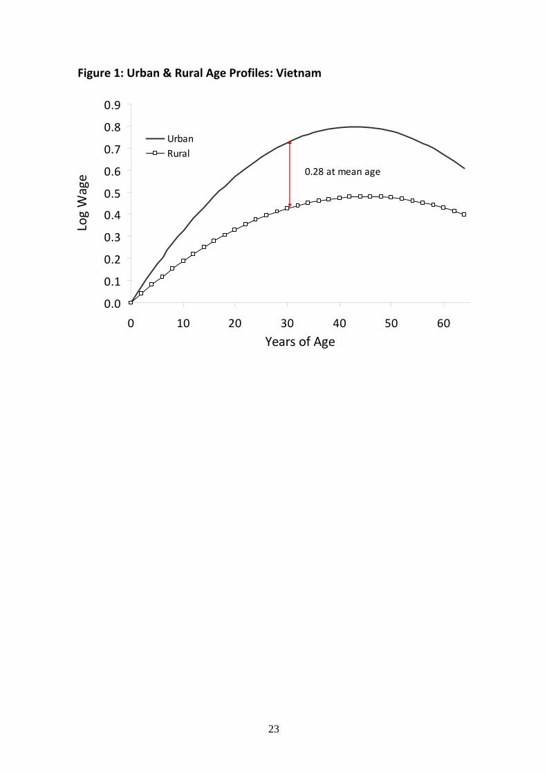
Figure 1: Urban & Rural Age Profiles: Vietnam
0.0
0.1
0.2
0.3
0.4
0.5
0.6
0.7
0.8
0.9
0 10 20 30 40 50 60
Years of Age
Log Wage
UrbanRural
0.28 at mean age
23

Table 3: Decomposition of Rural Non‐Agricultural – Agricultural Difference in Mean Log Wages
CountriesR2
NonAgricR2Agric Educ Public Occup Infra
Total Dueto Assets Age Educ Infra
Total Dueto Prices
ShareUnexplained
Sub‐Saharan AfricaGhana 627 124 0.4161 0.4512 0.39 0.07 0.05 0.00 0.03 0.15 1.36 ‐0.06 0.01 0.24 0.63Malawi 1892 7830 0.4245 0.1317 0.53 0.01 0.08 0.11 0.04 0.38 0.66 0.09 0.02 0.15 0.29Nigeria 1180 502 0.3043 0.2459 0.60 0.04 0.23 ‐0.03 0.04 0.30 1.32 ‐0.07 ‐0.01 0.30 0.50
South & East AsiaBangladesh 3314 3084 0.2288 0.3187 0.43 0.05 0.07 0.30 0.00 0.26 ‐0.08 0.04 0.00 0.17 0.40Indonesia 2232 1356 0.3696 0.2028 0.53 0.29 0.09 ‐0.12 0.06 0.27 0.25 ‐0.18 ‐0.02 0.26 0.49Nepal 3235 2833 0.1321 0.1304 0.54 0.02 ‐ 0.16 0.02 0.18 ‐0.04 0.02 0.00 0.36 0.67Vietnam 1879 1617 0.2165 0.2263 ‐0.11 0.02 ‐0.01 ‐0.03 0.04 ‐0.06 0.14 0.02 ‐0.01 ‐0.04 0.41
Eastern Europe & Central AsiaAlbania 572 102 0.2120 0.3192 ‐0.63 0.05 ‐0.03 ‐0.11 0.03 ‐0.11 ‐0.22 0.23 0.04 ‐0.52 0.83Bulgaria 493 150 0.2082 0.7010 ‐0.19 0.04 0.01 0.05 0.01 ‐0.06 0.38 ‐0.77 0.00 ‐0.14 0.71Tajikistan 930 2281 0.2648 0.2019 1.00 0.03 ‐0.03 0.28 0.00 0.48 0.33 0.65 0.01 0.53 0.53
Latin America & the CaribbeanEcuador 1368 1335 0.2278 0.0809 0.43 0.03 0.02 0.04 0.00 ‐0.01 ‐0.06 ‐0.23 0.00 0.44 1.03Guatemala 2020 2400 0.3250 0.1535 0.41 0.05 0.05 0.17 0.00 0.32 0.36 0.04 0.01 0.10 0.23Nicaragua 861 1063 0.1927 0.0978 0.39 0.07 ‐0.02 0.05 0.00 0.07 0.72 0.11 0.00 0.32 0.82Panama 1689 1265 0.3129 0.2072 0.52 0.05 0.01 ‐0.01 0.11 0.43 0.06 0.21 0.01 0.10 0.19
Averages 1592 1853 0.2740 0.2478 0.35 0.06 0.04 0.06 0.03 0.18 0.37 0.01 0.00 0.16 0.55Note: Public sector variable not available for Nepal. 0.47
LogWageGap
Due to Price Differences ("Unexplained")NonAgricSampleSize
AgricSampleSize
Due to Asset Differences ("Explained")
Weighted Average
24

Table 4: Decomposition of Rural Male – Female Difference in Mean Log Wages
Countries Male Female Male Female Educ Ind Occup Infra Age Educ InfraSub‐Saharan Africa
Ghana 496 229 0.3490 0.3845 0.58 0.06 0.05 0.02 0.02 0.26 0.19 0.04 ‐0.05 0.32 0.56Malawi 6056 3666 0.2642 0.1691 0.35 0.00 0.05 0.03 0.01 0.08 ‐0.06 0.00 0.00 0.26 0.76Nigeria 1252 430 0.2794 0.3122 0.14 ‐0.01 ‐0.01 ‐0.03 ‐0.02 ‐0.18 0.48 0.00 0.07 0.31 2.31
South & East AsiaBangladesh 3248 3150 0.3226 0.3067 0.04 0.03 0.00 0.02 0.00 0.02 0.65 0.00 0.00 0.02 0.56Indonesia 2475 1113 0.2844 0.3694 0.43 0.05 0.01 0.00 0.00 0.02 0.19 ‐0.03 0.00 0.40 0.94Nepal 2882 3186 0.2997 0.2782 0.04 0.03 0.00 0.00 0.00 0.02 0.18 ‐0.01 0.00 0.02 0.46Vietnam 2089 1407 0.2345 0.1980 0.20 0.01 0.04 ‐0.02 0.00 0.04 0.18 ‐0.02 0.01 0.15 0.78
Eastern Europe & Central AsiaAlbania 563 111 0.2648 0.3661 0.40 ‐0.04 0.12 ‐0.01 0.00 0.15 ‐0.23 0.47 ‐0.02 0.25 0.63Bulgaria 327 316 0.3765 0.3711 0.09 0.02 0.01 ‐0.04 0.00 ‐0.03 ‐0.25 ‐0.02 ‐0.01 0.12 1.30Tajikistan 1897 1314 0.3122 0.2461 0.61 0.02 0.10 0.07 0.01 0.28 0.02 ‐0.47 0.00 0.33 0.54
Latin America & the CaribbeanEcuador 2087 616 0.1611 0.1947 0.38 0.00 0.04 ‐0.05 0.00 0.02 1.16 ‐0.02 0.01 0.36 0.96Guatemala 3507 913 0.2882 0.3194 0.27 ‐0.01 ‐0.06 ‐0.01 0.00 ‐0.10 0.59 ‐0.05 0.00 0.37 1.37Nicaragua 1486 438 0.2388 0.2070 0.06 ‐0.05 ‐0.09 0.04 0.00 ‐0.09 ‐0.49 ‐0.03 0.00 0.15 2.59Panama 2271 683 0.3032 0.4161 ‐0.11 ‐0.04 0.07 ‐0.13 ‐0.07 ‐0.25 0.41 ‐0.21 0.01 0.14 ‐1.32
Averages 2188 1255 0.2842 0.2956 0.25 0.01 0.02 ‐0.01 0.00 0.02 0.22 ‐0.02 0.00 0.23 0.890.93
Share Unexplained
Due to Price Differences ("Unexplained")Due to Asset Differences ("Explained")Total Dueto Assets
Total Dueto Prices
Weighted Average
Log Wage Gap
Sample Size R2
25

Table 5: Decomposition of Urban Male – Female Difference in Mean Log Wages
Countries Male Female Male Female Educ Ind Occup Age EducSub‐Saharan Africa
Ghana98 567 224 0.3619 0.4839 0.31 ‐0.01 0.04 ‐0.01 0.06 0.88 ‐0.04 0.25 0.80Malawi04 1082 401 0.2950 0.4921 0.18 ‐0.05 0.05 ‐0.02 0.07 ‐1.15 0.01 0.11 0.59Nigeria04 872 372 0.3635 0.4403 0.30 0.01 0.06 ‐0.10 0.11 0.95 0.07 0.19 0.64
South & East AsiaBangladesh00 2172 2206 0.4076 0.4316 0.21 0.07 0.01 0.09 0.19 ‐0.30 ‐0.05 0.02 0.08Indonesia00 3154 1760 0.3445 0.4833 0.37 0.02 0.01 ‐0.04 0.00 0.39 ‐0.35 0.37 0.99Nepal03 1194 1177 0.2239 0.1938 0.09 0.02 0.00 0.01 0.09 ‐0.23 0.00 ‐0.01 ‐0.06Vietnam98 1216 919 0.3407 0.3431 0.23 0.01 0.04 0.00 0.06 0.60 ‐0.21 0.17 0.75
Eastern Europe & Central AsiaAlbania05 1031 697 0.0959 0.2276 0.29 ‐0.03 0.03 ‐0.04 ‐0.01 0.35 ‐0.41 0.31 1.04Bulgaria01 979 1091 0.1883 0.1866 0.15 0.00 0.02 ‐0.02 ‐0.02 0.03 0.12 0.17 1.15Tajikistan03 735 473 0.2270 0.2751 0.48 0.01 0.03 0.01 0.07 ‐1.20 0.50 0.41 0.86
Latin America & the CaribbeanEcuador95 2682 1687 0.2350 0.2740 0.36 ‐0.03 0.04 ‐0.01 ‐0.02 ‐0.03 ‐0.06 0.38 1.05Guatemala00 3000 1753 0.4518 0.4291 0.23 ‐0.01 0.00 ‐0.03 ‐0.02 ‐0.51 ‐0.09 0.25 1.09Nicaragua01 1950 1206 0.3018 0.2957 0.11 ‐0.06 0.08 ‐0.04 ‐0.06 0.65 0.08 0.17 1.58Panama03 2603 1888 0.3711 0.4207 0.12 ‐0.05 0.02 ‐0.08 ‐0.15 0.13 ‐0.11 0.26 2.22
Averages 1660 1132 0.3006 0.3555 0.25 ‐0.01 0.03 ‐0.02 0.03 0.04 ‐0.04 0.22 0.91Notes: (1) Public dummy in Nepal 2003 is not available. 0.89
Sample Size R2 Total Dueto Assets
Share Unexplained
Total Dueto Prices
Due to Asset Differences ("Explained") Due to Price Differences ("Unexplained")LogWageGap
Weighted Average
26

Figure 2: Male and Female Age Profiles: Rural Nepal
0.0
0.1
0.2
0.3
0.4
0 10 20 30 40 50 60Age
Pred
icted Log Wage
Male
Female
0.18 at mean age
27
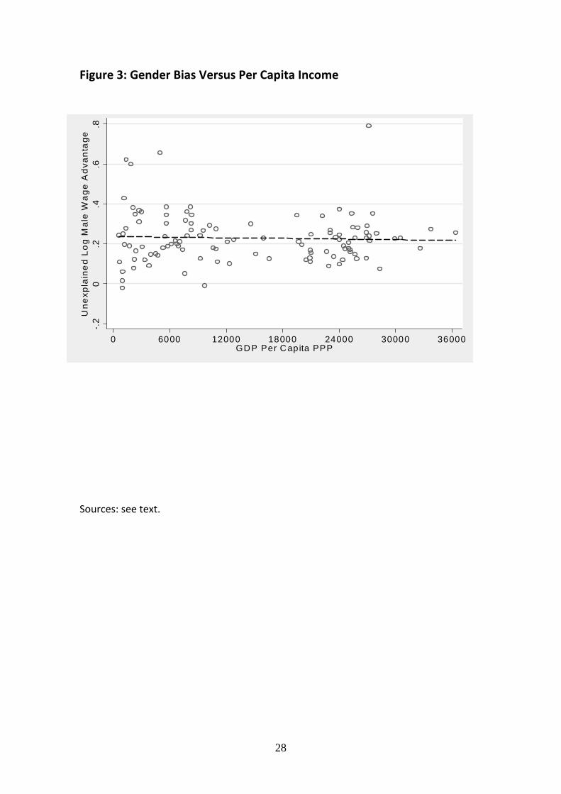
Figure 3: Gender Bias Versus Per Capita Income
-.2
0.2
.4.6
.8U
nexp
lain
ed L
og M
ale
Wa
ge A
dvan
tage
0 6000 12000 18000 24000 30000 36000GDP Per Capita PPP
Sources: see text.
28
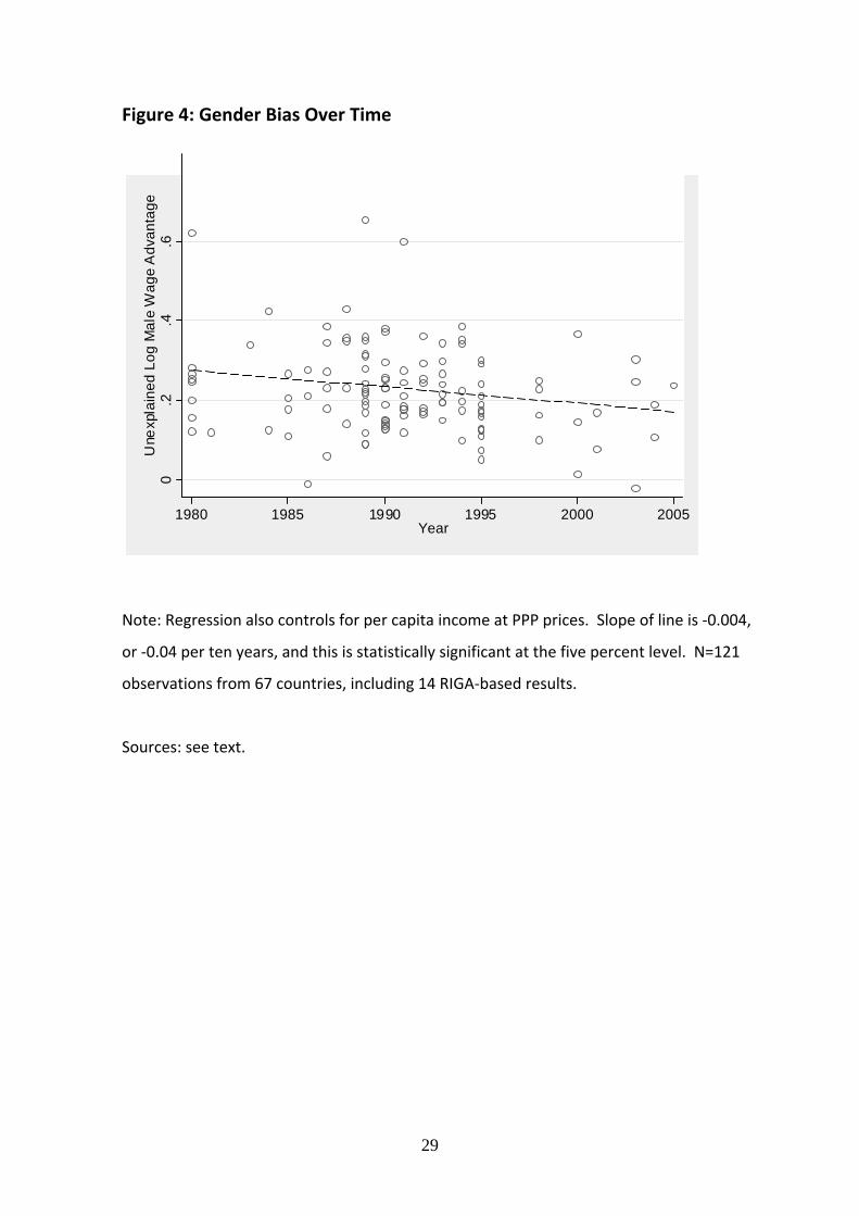
Figure 4: Gender Bias Over Time
0
.2.4
.6U
nexp
lain
ed L
og M
ale
Wag
e A
dvan
tage
1980 1985 1990 1995 2000 2005Year
Note: Regression also controls for per capita income at PPP prices. Slope of line is ‐0.004,
or ‐0.04 per ten years, and this is statistically significant at the five percent level. N=121
observations from 67 countries, including 14 RIGA‐based results.
Sources: see text.
29

Appendix
Table A1: Survey Years, Sources, and Sample Sizes
Urban Rural Non_Ag Ag
Sub‐Saharan AfricaGhana, 1998 Ghana Living Standards Survey Round 3 791 751 627 124Malawi, 2004 Integrated Household Survey 2 1483 9722 1892 7830Nigeria, 2004 Living Standards Survey 1244 1682 1180 502
South & East AsiaBangladesh, 2000 Household Income‐Expenditure Survey 4378 6398 3314 3084Indonesia, 2000 Family Life Survey Wave 3 4914 3588 2232 1356Nepal, 2003 Living Standards Survey 2 2371 6068 3235 2833Vietnam, 1998 Living Standards Survey 2135 3496 1879 1617
Eastern Europe & Central AsiaAlbania, 2005 Living Standards Measurement Survey 1728 674 572 102Bulgaria, 2001 Integrated Household Survey 2070 643 493 150Tajikistan, 2003 Living Standards Survey 1208 3211 930 2281
Latin America & the CaribbeanEcuador, 1995 Estudio de Condiciones de Vida 4369 2703 1368 1335Guatemala, 2000 Encuesta de Condiciones de Vida 4753 4420 2020 2400Nicaragua, 2001 Encuesta de Medición de Niveles de Vida 3156 1924 861 1063Panama, 2003 Encuesta de Niveles de Vida 4491 2954 1689 1265
Averages 2792 3445 1592 1853
Countries & Years Name of SurveyRuralTotal
30

Table A2: Comparison of Daily and Hourly Log Wage Gaps
Hourly Wage Daily Wage Hourly Wage Daily Wage Hourly Wage Daily Wage Hourly Wage Daily WageSouth & East Asia
Bangladesh00 0.23 0.29 0.37 0.43 0.04 0.04 0.20 0.21Nepal03 0.30 0.28 0.60 0.54 0.04 0.04 0.06 0.09Vietnam98 0.35 0.30 0.01 ‐0.11 0.17 0.20 0.17 0.23
Eastern Europe & Central AsiaAlbania05 ‐0.04 ‐0.05 ‐0.57 ‐0.63 0.32 0.40 0.22 0.29Tajikistan03 0.94 0.96 1.05 1.00 0.56 0.61 0.31 0.48
Latin America & the Caribbean*Ecuador95 0.42 0.46 0.25 0.31 0.41 0.44 0.27 0.37Guatemala00 0.54 0.53 0.37 0.40 0.14 0.29 0.06 0.24Nicaragua01 0.35 0.45 0.33 0.47 0.01 0.00 0.02 0.10Panama03 0.51 0.54 0.48 0.52 ‐0.15 ‐0.15 0.10 0.11
Average 0.40 0.42 0.32 0.33 0.17 0.21 0.16 0.24
Note: *Differentials in these countries refer only to main and secondary jobs (job 1 and job 2) because hours data were lacking for jobs 3 and 4.
Urban ‐ Rural Rural Male ‐ Female Urban Male ‐ FemaleNonAgric ‐ Agric
31

Table A3: Summary of Oaxaca Results for Urban/Rural and Rural Non‐Agricultural/Agricultural Wage Gaps: Hourly Wages
Log Wage Gap
Assets PricesShare Due to Prices
Log Wage Gap
Assets PricesShare Due to Prices
South & East AsiaBangladesh00 0.23 0.13 0.10 0.44 0.37 0.22 0.16 0.42Nepal03 0.30 0.29 0.01 0.03 0.60 0.18 0.42 0.70Vietnam98 0.35 0.14 0.20 0.59 0.01 0.00 0.00 0.33
Eastern Europe & Central AsiaAlbania05 ‐0.04 ‐0.06 0.02 ‐0.48 ‐0.57 ‐0.09 ‐0.49 0.84Tajikistan03 0.94 0.50 0.45 0.47 1.05 0.43 0.61 0.59
Latin America & the Caribbean*Ecuador95 0.42 0.21 0.21 0.49 0.25 ‐0.20 0.45 1.80Guatemala00 0.54 0.47 0.07 0.13 0.37 0.39 ‐0.02 ‐0.04Nicaragua01 0.35 0.30 0.05 0.14 0.33 0.20 0.13 0.40Panama03 0.51 0.28 0.23 0.45 0.48 0.37 0.11 0.24
Average 0.40 0.25 0.15 0.25 0.32 0.17 0.15 0.590.37 0.48
Note: *Differentials in these countries refer only to main and secondary jobs (job 1 and job 2) as hours data were lacking for jobs 3 and 4.
NonAgric ‐ Agric (Rural)Urban ‐ Rural
Weighted average Weighted average
32

Table A4: Summary of Oaxaca Results for Rural and Urban Male/Female Wage Gaps: Hourly Wages
Log Wage Gap
Assets PricesShare Due to Prices
Log Wage Gap
Assets PricesShare Due to Prices
South & East AsiaBangladesh00 0.04 0.02 0.02 0.57 0.20 0.19 0.02 0.08Nepal03 0.04 0.02 0.02 0.54 0.06 0.08 ‐0.02 ‐0.39Vietnam98 0.17 0.01 0.16 0.94 0.17 0.01 0.16 0.96
Eastern Europe & Central AsiaAlbania05 0.32 0.09 0.23 0.72 0.22 ‐0.02 0.24 1.10Tajikistan03 0.56 0.27 0.29 0.51 0.31 0.06 0.25 0.79
Latin America & the Caribbean*Ecuador95 0.41 0.02 0.39 0.94 0.27 ‐0.03 0.30 1.11Guatemala00 0.14 ‐0.16 0.30 2.13 0.06 ‐0.09 0.15 2.53Nicaragua01 0.01 ‐0.10 0.12 9.11 0.02 ‐0.05 0.08 3.16Panama03 ‐0.15 ‐0.36 0.21 ‐1.38 0.10 ‐0.20 0.30 2.93
Average 0.17 ‐0.02 0.19 1.57 0.16 ‐0.01 0.16 1.361.13 1.04
Note: *Differentials in these countries refer only to main and secondary jobs (job 1 and job 2) as hours data were lacking for jobs 3 and 4.
Weighted average Weighted average
Rural Male‐Female Urban Male‐Female
33
ESA Working Papers
WORKING PAPERS The ESA Working Papers are produced by the Agricultural Development Economics Division (ESA) of the Economic and Social Development Department of the United Nations Food and Agriculture Organization (FAO). The series presents ESA’s ongoing research. Working papers are circulated to stimulate discussion and comments. They are made available to the public through the Division’s website. The analysis and conclusions are those of the authors and do not indicate concurrence by FAO. ESA The Agricultural Development Economics Division (ESA) is FAO’s focal point for economic research and policy analysis on issues relating to world food security and sustainable development. ESA contributes to the generation of knowledge and evolution of scientific thought on hunger and poverty alleviation through its economic studies publications which include this working paper series as well as periodic and occasional publications.
Agricultural Development Economics Division (ESA)
The Food and Agriculture Organization Viale delle Terme di Caracalla
00153 Rome Italy
Contact: Office of the Director
Telephone: +39 06 57054358 Facsimile: + 39 06 57055522 Website: www.fao.org/es/esa
e-mail: [email protected]
34
Top Related