


Languages
Pages
Legal


Degeneracy loci and G2 flags
by
David E. Anderson
A dissertation submitted in partial fulfillmentof the requirements for the degree of
Doctor of Philosophy(Mathematics)
in the University of Michigan2009
Doctoral Committee:
Professor William Fulton, ChairProfessor Sergey FominProfessor Robert K. LazarsfeldAssociate Professor James P. TappendenAssistant Professor Benjamin J. Howard

1
2 3
4
5
67

c© David E. Anderson2009

Acknowledgements
Graduate school, for me, has been an intense and sometimes difficult experience.
I’d like to start by thanking all the friends in Ann Arbor who made that expe-
rience more fun, especially Elizabeth Coe, Leo Goldmakher, Hester Graves, Mark
Iwen, Ryan Kinser, Mike Lieberman, and Craig Spencer. Special thanks also to my
parents and sister for stomaching a couple over-zealous explanations of certain agro-
mathematical metaphors. Most of all, I thank Liz Vivas for her love and support
through both the brightest and darkest times of the last few years.
The math department at the University of Michigan is a remarkably congenial
place to study and work, and I want to thank all the people who make it so. It
has been a great pleasure to learn mathematics from and with many people here
and elsewhere, especially Karcsi Boroczky, Chuck Cadman, Renzo Cavalieri, Linda
Chen, Brian Conrad, Igor Dolgachev, Danny Gillam, Milena Hering, Ben Howard,
Robert Lazarsfeld, Leonardo Mihalcea, Ezra Miller, Mircea Mustata, Karen Smith,
Alan Stapledon, John Stembridge, Tamas Szamuely, Agnes Szilard, Michael Thad-
deus, Giancarlo Urzua, Ravi Vakil, and Alex Yong. I want to thank Sam Payne
and Julianna Tymoczko in particular for encouraging my interest in combinatorial
algebraic geometry, and for their advice along the way.
While working on this thesis, I benefitted from emails and discussions with Robert
Bryant, Skip Garibaldi, Bill Graham, Gopal Prasad, and Richard Rimanyi. I would
also like to thank all my committee members for their time and energy.
I first learned about Schubert varieties from Sergey Fomin, and his lectures in-
spired me to learn about Schubert calculus. I thank him for teaching me how to think
about combinatorics, as well as for his candid advice and comments on manuscripts.
ii

Finally, I am deeply grateful to Bill Fulton for generously sharing his time and
thoughts, for suggesting this project and others, for his encouragement while I pursued
them, and for detailed comments on the manuscripts that resulted. He has given me
invaluable advice at every stage of graduate school, and I thank him for showing me
how to be a mathematician.
iii

Table of Contents
Acknowledgements ii
List of Appendices v
Chapter 1. Introduction 11.1. Overview 5
Chapter 2. Octonions and compatible forms 162.1. Standard facts 172.2. Forms 192.3. Octonion bundles 262.4. Another construction 28
Chapter 3. Isotropic flags and flag bundles 333.1. Topology of G2 flags 333.2. Cohomology of flag bundles 37
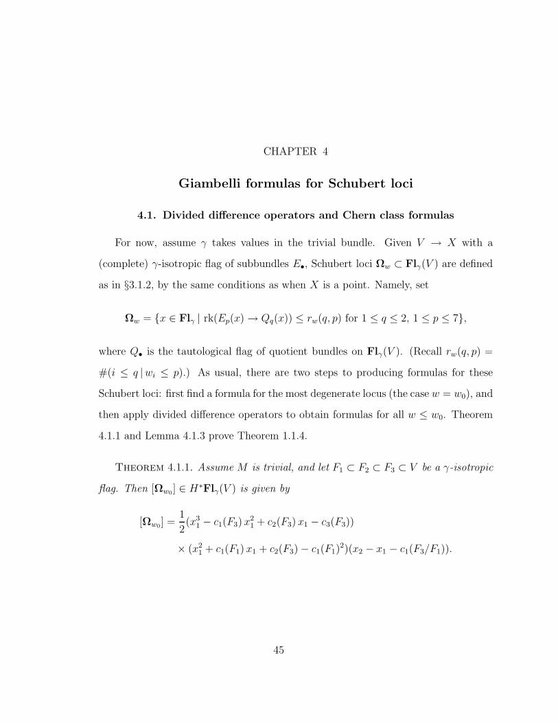
Chapter 4. Giambelli formulas for Schubert loci 454.1. Divided difference operators and Chern class formulas 454.2. Variations 49
Chapter 5. Degeneracy of morphisms 555.1. Triality symmetry 565.2. Orbits 585.3. Graphs 62
Chapter 6. Characteristic two 676.1. Forms and octonions 676.2. Forms and homogeneous spaces 72
Appendices 74
Bibliography 125
iv

List of Appendices
Appendix A. Lie theory 74
Appendix B. Triality 87
Appendix C. Graphs and symmetry 97
Appendix D. Tables 107
Appendix E. Integral Chow rings of quadric bundles 120
v

CHAPTER 1
Introduction
Let V be an n-dimensional vector space. The flag variety F l(V ) parametrizes all
complete flags in V , i.e., saturated chains of subspaces E• = (E1 ⊂ E2 ⊂ · · · ⊂ En =
V ) (with dim Ei = i). Fixing a flag F• allows one to define Schubert varieties in F l(V )
as the loci of flags satisfying certain incidence conditions with F•; there is one such
Schubert variety for each permutation of 1, . . . , n. This generalizes naturally to the
case where V is a vector bundle and F• is a flag of subbundles. Here one has a flag
bundle Fl(V ) over the base variety, whose fibers are flag varieties, with Schubert loci
defined similarly by incidence conditions. Formulas for the cohomology classes of these
Schubert loci, as polynomials in the Chern classes of the bundles involved, include
the classical Thom–Porteous–Giambelli and Kempf–Laksov formulas (see [Fu1]).
The above situation is “type A,” in the sense that F l(V ) is isomorphic to the ho-
mogeneous space SLn/B (with B the subgroup of upper-triangular matrices). There
are straightforward generalizations to the other classical types (B, C, D): here the
vector bundle V is equipped with a symplectic or nondegenerate symmetric bilin-
ear form, and the flags are required to be isotropic with respect to the given form.
Schubert loci are defined as before, with one for each element of the corresponding
Weyl group. The problem of finding formulas for their cohomology classes has been
studied by Harris–Tu [Ha-Tu], Jozefiak–Lascoux–Pragacz [Jo-La-Pr], and Fulton
[Fu2, Fu3], among others.
1

One is naturally led to consider the analogous problem in the five remaining
Lie types. In exceptional types, however, it is not so obvious how the Lie-theoretic
geometry of G/B generalizes to the setting of vector bundles in algebraic geometry.
The primary goal of this thesis is to carry this out for type G2.
To give a better idea of the difference between classical and exceptional types, let
us describe the classical problem in slightly more detail. The flag bundles are the
universal cases of general degeneracy locus problems in algebraic geometry. Specifi-
cally, let V be a vector bundle of rank n on a variety X, and let ϕ : V ⊗ V → k be
a symplectic or nondegenerate symmetric bilinear form (or the zero form). If E• and
F• are general flags of isotropic subbundles of V , the problem is to find formulas in
H∗X for the degeneracy locus
Dw = x ∈ X | dim(Fp(x) ∩ Eq(x)) ≥ rw w0(q, p),
in terms of the Chern classes of the line bundles Eq/Eq−1 and Fp/Fp−1, for all p and
q. (Here w is an element of the Weyl group, considered as a permutation via an
embedding in the symmetric group Sn; w0 is the longest element, corresponding to
the permutation n n − 1 · · · 1; and rw(q, p) = #i ≤ q |w(i) ≤ p is a nonnegative
integer depending on w, p, and q.) Such formulas have a wide range of applications:
for example, they appear in the theory of special divisors and variation of Hodge
structure on curves in algebraic geometry [Ha-Tu, Pa-Pr], and they are used to study
singularities of smooth maps in differential geometry (work of Feher and Rimanyi).
They are also of interest in combinatorics (Lascoux–Schutzenberger, Fomin–Kirillov,
Pragacz, Kresch–Tamvakis). See [Fu-Pr] for a more detailed account of the history.
In this thesis, we pose and solve the corresponding problem in type G2:
2

Let V → X be a vector bundle of rank 7, equipped with a nondegen-erate alternating trilinear form γ :
∧3 V → L, for a line bundle L.Let E• and F• be general flags of γ-isotropic subbundles of V , andlet
Dw = x ∈ X | dim(Fp(x) ∩ Eq(x)) ≥ rw w0(q, p),
where w is an element of W (G2) (the dihedral group with 12 ele-ments), and rw(q, p) is a certain nonnegative integer. Find a for-mula for [Dw] in H∗X, in terms of the Chern classes of the bundlesinvolved.
(The meaning of “nondegenerate” and “γ-isotropic” will be explained below (§§1.1.1–
1.1.2), as will the precise definition of Dw (§1.1.5).) Proofs and variations of the
formulas are given in Chapter 4; the formulas themselves are listed in Appendix D.2.
Formulas for degeneracy loci are closely related to Giambelli formulas for equivari-
ant classes of Schubert varieties in the equivariant cohomology of the corresponding
flag variety. We will usually use the language of degeneracy loci, but we discuss the
connection with equivariant cohomology in §1.1.6. In brief, the two perspectives are
equivalent when det V and L are trivial line bundles.
Another notion of degeneracy loci is often useful. Let ϕ : E → F be a morphism of
vector bundles on X, subject to some symmetry hypothesis; for example, if F = E∗,
one may require that ϕ∗ : E∗∗ = E → E∗ be equal to ϕ. In this setup, there is a
degeneracy locus
Dr = Dr(ϕ) = x ∈ X | rk(ϕ(x) : E(x) → F (x)) ≤ r,
and one can ask for formulas for such loci as well. (The expected codimension of Dr
depends on the type of symmetry one imposes on ϕ.) In classical types, this problem
is equivalent to the “incidence” version discussed above, by replacing ϕ with its graph
in V = E ⊕ F . Indeed, many of the works cited above deal with morphisms rather
than subbundles.
3

Once again, it makes sense to consider this problem in exceptional types, but the
appropriate notion of symmetry is somewhat more subtle than in classical types. In
Appendix C, we introduce a general notion of symmetry corresponding to a homo-
geneous space G/P , and discuss its relation to the graph of a morphism. Chapter 5
gives formulas for degeneracy loci of triality-symmetric morphisms, which is the G2
case; see §1.1.7 for the definition. Here we will deal with equivariant cohomology more
directly: in the spirit of [Fe-Ne-Ri], these formulas come from equivariant classes of
orbit closures in a vector space.
When the base X is a point, so V is a vector space and the flag bundle is just
the flag variety G/B, most of the results have been known for some time; essentially
everything can be done using the general tools of Lie theory. For example, a pre-
sentation of H∗(G/B, Z) was given by Bott and Samelson [Bo-Sa], and (different)
formulas for Schubert classes in H∗(G/B, Q) appear in [BGG]. Since this thesis also
aims to present a concrete, unified perspective on the G2 flag variety, accessible to
general algebraic geometers, we wish to emphasize geometry over Lie theory: we are
describing a geometric situation from which type-G2 groups arise naturally. Reflecting
this perspective, we use Lie-theoretic arguments sparingly, avoiding them altogether
in the first four chapters. Appendix A collects the basic representation-theoretic facts
we use, and relates our geometric constructions with the general Lie-theoretic ones.
In Appendix B, we give a brief exposition of triality and its relation to the G2 flag
variety.
Various constructions of exceptional-type flag varieties have been given using tech-
niques from algebra and representation theory; those appearing in [La-Ma], [Il-Ma],
and [Ga2] have a similar flavor to the one presented here. A key feature of our de-
scription is that the data parametrized by the G2 flag variety naturally determine
4

a complete flag in a 7-dimensional vector space, much as isotropic flags in classical
types determine complete flags by taking orthogonal complements. The fundamental
facts that make this work are Proposition 1.1.2 and its cousins, Corollary 2.2.10 and
Propositions 2.3.2 and 2.3.3.
Notation and conventions. Unless otherwise indicated, the base field k will have
characteristic not 2 and be algebraically closed (although a quadratic extension of
the prime field usually suffices). Angle brackets denote the span of enclosed vectors:
〈x, y, z〉 := spanx, y, z. If X → Y is a morphism and V is a vector bundle on Y , we
will often write V for the vector bundle pulled back to X; if x is a point of X, V (x)
denotes the fiber over x. If V is a vector space and E is a subspace, [E] denotes the
corresponding point in an appropriate Grassmannian. For a group G, if X is a right
G-space and Y is a left G-space, we write X ×G Y for the “balanced quotient,” given
by the equivalence relation (x, g · y) ∼ (x · g, y).
We generally use the notation and language of (singular) cohomology, but this
should be read as Chow cohomology for ground fields other than C. (Since the
varieties whose cohomology we compute are rational homogeneous spaces or fibered
in homogeneous spaces, the distinction is not significant.)
1.1. Overview
We begin with an overview of our description of the G2 flag variety and statements
of the main results. Proofs and details are given in later sections.
1.1.1. Compatible forms. Let V be a k-vector space. Let β be a nondegenerate
symmetric bilinear form on V , and let γ be an alternating trilinear form, i.e., γ :∧3 V → k. Write v 7→ v† for the isomorphism V → V ∗ defined by β, and ϕ 7→ ϕ† for
5

the inverse map V ∗ → V . (Explcitly, these are defined by v†(u) = β(v, u) and ϕ(u) =
(ϕ†, u) for any u ∈ V .) Our constructions are based on the following definitions:
Definition 1.1.1. Call the forms γ and β compatible if
2 γ(u, v, γ(u, v, ·)†) = β(u, u)β(v, v)− β(u, v)2(1.1.1)
for all u, v ∈ V . An alternating trilinear form γ :∧3 V → k is nondegenerate if
there exists a compatible nondegenerate symmetric bilinear form on V .
The meaning of the strange-looking relation (1.1.1) will be explained in §2; see
Proposition 2.2.1. (The factor of 2 is due to our convention that a quadratic norm and
corresponding bilinear form are related by β(u, u) = 2 N(u).) A pair of compatible
forms is equivalent to a composition algebra structure on k ⊕ V (see §2). Since a
composition algebra must have dimension 1, 2, 4, or 8 over k (by Hurwitz’s theorem),
it follows that nondegenerate trilinear forms exist only when V has dimension 1,
3, or 7. In each case, there is an open dense GL(V )-orbit in∧3 V ∗ consisting of
nondegenerate forms. When dim V = 1, the only alternating trilinear form is zero,
and any nonzero bilinear form is compatible with it. When dim V = 3, an alternating
trilinear form is a scalar multiple of the determinant, and given a nondegenerate
bilinear form, it is easy to show that there is a unique compatible trilinear form up
to sign.
When dim V = 7, it is less obvious that∧3 V ∗ has an open GL(V )-orbit, especially
if char(k) = 3, but it is still true (Proposition A.2.2). The choice of γ determines β
uniquely up to scalar — in fact, up to a cube root of unity (see Proposition A.2.6).
Associated to any alternating trilinear form γ on a seven-dimensional vector space
V , there is a canonical map Bγ : Sym2 V →∧7 V ∗, determining (up to scalar) a
bilinear form βγ . We will give the formula for char(k) 6= 3 here. Following Bryant
6

[Br], we define Bγ by
Bγ(u, v) = −1
3γ(u, ·, ·) ∧ γ(v, ·, ·) ∧ γ,(1.1.2)
where γ(u, ·, ·) :∧2 V → k is obtained by contracting γ with u. Choosing an isomor-
phism∧7 V ∗ ∼= k yields a symmetric bilinear form βγ. If βγ is nondegenerate, then a
scalar multiple of it is compatible with the trilinear form γ; thus γ is nondegenerate
if and only if βγ is nondegenerate. The form βγ is defined in characteristic 3, as well,
and the statement still holds (see Lemma 2.2.7 and its proof).
1.1.2. Isotropic spaces. For the rest of this section, assume dim V = 7. Given
a nondegenerate trilinear form γ on V , say a subspace F of dimension at least 2
is γ-isotropic if γ(u, v, ·) ≡ 0 for all u, v ∈ F . (That is, the map F ⊗ F → V ∗
induced by γ is zero.) Say a vector or a 1-dimensional subspace is γ-isotropic if it
is contained in a 2-dimensional γ-isotropic space. If β is a compatible bilinear form,
every γ-isotropic subspace is also β-isotropic (Lemma 2.2.3); as usual, this means β
restricts to zero on F . Since β is nondegenerate, a maximal β-isotropic subspace has
dimension 3.
Proposition 1.1.2. For any (nonzero) isotropic vector u ∈ V , the space
Eu = v | 〈u, v〉 is γ-isotropic
is three-dimensional and β-isotropic. Moreover, every two-dimensional γ-isotropic
subspace of Eu contains u.
The proof is given at the end of §2.2. The proposition implies that a maximal γ-
isotropic subspace has dimension 2, and motivates the central definition:
7

Definition 1.1.3. A γ-isotropic flag (or G2 flag) in V is a chain
F1 ⊂ F2 ⊂ V
of γ-isotropic subspaces, of dimensions 1 and 2. The variety parametrizing γ-isotropic
flags is called the γ-isotropic flag variety (or G2 flag variety), and denoted F lγ(V ).
The γ-isotropic flag variety is a smooth, six-dimensional projective variety (Propo-
sition 3.1.1). See §A.4 for its description as a homogeneous space.
Proposition 1.1.2 shows that a γ-isotropic flag has a unique extension to a complete
flag in V : set F3 = Eu for u spanning F1, and let F7−i be the orthogonal space
F⊥i , with respect to a compatible form β. (Since a compatible form is unique up
to scalar, this is independent of the choice of β.) This defines a closed immersion
F lγ(V ) → F lβ(V ) ⊂ F l(V ), where F lβ(V ) and F l(V ) are the (classical) type B and
type A flag varieties, respectively.
From the definition, there is a tautological sequence of vector bundles on F lγ(V ),
S1 ⊂ S2 ⊂ V,
and this extends to a complete γ-isotropic flag of bundles
S1 ⊂ S2 ⊂ S3 ⊂ S4 ⊂ S5 ⊂ S6 ⊂ V
by the proposition. Similarly, there are universal quotient bundles Qi = V/S7−i.
1.1.3. Bundles. Now let V → X be a vector bundle of rank 7, and let L be a
line bundle on X. An alternating trilinear form γ :∧3 V → L is nondegenerate
if it is locally nondegenerate on fibers. Equivalently, we may define the Bryant form
8

Bγ : Sym2 V → det V ∗⊗L⊗3 by Equation (1.1.2), and γ is nondegenerate if and only
if Bγ is (so Bγ defines an isomorphism V ∼= V ∗ ⊗ det V ∗ ⊗ L⊗3).
A subbundle F of V is γ-isotropic if each fiber F (x) is γ-isotropic in V (x); for
F of rank 2, this is equivalent to requiring that the induced map F ⊗ F → V ∗ ⊗ L
be zero. If F1 ⊂ V is γ-isotropic, the bundle EF1 = ker(V → F ∗1 ⊗ V ∗ ⊗ L) has rank
3 and is isotropic for Bγ. (If u is a vector in a fiber F1(x), then EF1(x) = Eu, in the
notation of §1.1.2.)
Given a nondegenerate form γ on V , there is a γ-isotropic flag bundle Flγ(V ) →
X, with fibers F lγ(V (x)). This comes with universal γ-isotropic subbundles Si and
quotient bundles Qi, as before.
1.1.4. Chern class formulas. In the setup of §1.1.3, one has Schubert loci
Ωw ⊆ Flγ(V ) indexed by the Weyl group. There is an embedding of W = W (G2)
in the symmetric group S7 such that the permutation corresponding to w ∈ W
is determined by its first two values. We identify w with this pair of integers, so
w = w1 w2; see §A.3 for more on the Weyl group. As in classical types, we set
rw(q, p) = #i ≤ q |w(i) ≤ p.(1.1.3)
Given a fixed γ-isotropic flag F• on X, the Schubert loci are defined by
Ωw = x ∈ Flγ(V ) | rk(Fp → Qq) ≤ rw(q, p) for 1 ≤ p ≤ 7, 1 ≤ q ≤ 2.
These are locally trivial fiber bundles, whose fibers are Schubert varieties in F lγ(V (x)).
The G2 divided difference operators ∂s and ∂t act on Λ[x1, x2], for any ring
Λ, by
∂s(f) =f(x1, x2) − f(x2, x1)
x1 − x2;(1.1.4)
9

∂t(f) =f(x1, x2) − f(x1, x1 − x2)
−x1 + 2x2
.(1.1.5)
If w ∈ W has reduced word w = s1 · s2 · · · sℓ (where si is the simple reflection s or t),
then define ∂w to be the composition ∂s1 · · · ∂sℓ. This is independent of the choice
of word; see §A.5. (As mentioned in §A.3, each w ∈ W (G2) has a unique reduced
word, with the exception of w0, so independence of choice is actually lack of choice
in this case.) These formulas also define operators on H∗Flγ(V ). (See §4.1.)
Let V be a vector bundle of rank 7 on X equipped with a nondegenerate form
γ :∧3 V → kX , and assume det V is trivial. Let F1 ⊂ F2 ⊂ · · · ⊂ V be a complete
γ-isotropic flag in V . Set y1 = c1(F1), y2 = c1(F2/F1). Let Flγ(V ) → X be the flag
bundle, and set x1 = −c1(S1) and x2 = −c1(S2/S1), where S1 ⊂ S2 ⊂ V are the
tautological bundles.
Theorem 1.1.4. We have
[Ωw] = Pw(x; y),
where Pw = ∂w0 w−1Pw0, and
Pw0(x; y) =1
2(x3
1 − 2 x21 y1 + x1 y2
1 − x1 y22 + x1 y1 y2 − y2
1 y2 + y1 y22)
× (x21 + x1 y1 + y1 y2 − y2
2)(x2 − x1 − y2).
in H∗(Flγ(V ), Z). (Here w0 is the longest element of the Weyl group.)
The proof is given in §4.1, along with a discussion of alternative formulas, including
ones where γ takes values in M⊗3 for an arbitrary line bundle M .
1.1.5. Degeneracy loci. Returning to the problem posed in the introduction,
let V be a rank 7 vector bundle on a variety X, with nondegenerate form γ and two
10

(complete) γ-isotropic flags of subbundles F• and E•. The first flag, F•, allows us
to define Schubert loci in the flag bundle Flγ(V ) as in §1.1.4. The second flag, E•,
determines a section s of Flγ(V ) → X, and we define degeneracy loci as scheme-
theoretic inverse images under s:
Dw = s−1Ωw ⊂ X.
When X is Cohen-Macaulay and Dw has expected codimension (equal to the length
of w; see §A.3), we have
[Dw] = s∗[Ωw] = Pw(x; y)(1.1.6)
in H∗X, where xi = −c1(Ei/Ei−1) and yi = c1(Fi/Fi−1). More generally, this polyno-
mial defines a class supported on Dw, even without assumptions on the singularities
of X or the genericity of the flags F• and E•; see [Fu1] or [Fu-Pr, App. A] for the
intersection-theoretic details.
1.1.6. Equivariant cohomology. Now return to the case where V is a 7-dimensional
vector space. One can choose a basis f1, . . . , f7 such that Fi = 〈f1, . . . , fi〉 forms a
complete γ-isotropic flag in V , and let T = (k∗)2 act on V ∼= k7 by
(z1, z2) 7→ diag(z1, z2, z1z−12 , 1, z−1
1 z2, z−12 , z−1
1 ).
Write t1 and t2 for the corresponding weights. Then T preserves γ and acts on F lγ(V ).
The total equivariant Chern class of V is cT (V ) = (1 − t21)(1 − t22)(1 − (t1 − t2)2), so
we have
H∗T (F lγ(V ), Z[1
2]) = Z[1
2][x1, x2, t1, t2]/(r2, r4, r6),
11

with the relations r2i = ei(x21, x2
2, (x1 − x2)2) − ei(t
21, t22, (t1 − t2)
2). A presentation
with Z coefficients can be deduced from Theorem 3.2.4; see Remark 3.2.5.
Theorem 1.1.4 yields an equivariant Giambelli formula:
[Ωw]T = Pw(x; t) in H∗T F lγ.
In fact, this formula holds with integer coefficients: the Schubert classes form a basis
for H∗T (F lγ , Z) over Z[t1, t2], so in particular there is no torsion, and H∗
T (F lγ, Z)
includes in H∗T (F lγ, Z[1
2]).
Given an equivariant Giambelli formula, one can easily find the localization of a
Schubert class [Ωw]T at a fixed point e(v) and compute the multiplication table of
H∗T (F lγ) with respect to the Schubert basis. These computations are given in §D.3
and §D.4.
The equivariant geometry of F lγ is closely related to the degeneracy loci problem;
we briefly describe the connection. In the setup of §1.1.5, assume V has trivial
determinant and γ has values in the trivial bundle, so the structure group is G = G2.
The data of two γ-isotropic flags in V gives a map to the classifying space BB×BGBB,
where B ⊂ G is a Borel subgroup, and there are universal degeneracy loci Ωw in this
space. On the other hand, there is an isomorphism BB ×BG BB ∼= EB ×B (G/B),
carrying Ωw to EB ×B Ωw. Since H∗T (F lγ) = H∗(EB ×B (G/B)), and [Ωw]T =
[EB×B Ωw], a Giambelli formula for [Ωw]T is equivalent to a degeneracy locus formula
for this situation. One may then use equivariant localization to verify a given formula;
this is essentially the approach taken in [Gr2].
1.1.7. Triality-symmetric morphisms. A nondegenerate skew-sym-metric bi-
linear form on a vector space V of dimension 2n gives rise to a duality involution of
12

the (type A) Grassmannian Gr(n, V ) whose fixed locus is the Lagrangian Grass-
mannian LG(n, V ) ⊆ Gr(n, V ). If E ⊂ V is an isotropic n-dimensional subspace,
corresponding to a point [E] ∈ LG(n, V ), then V = E ⊕ E∗ and the tangent spaces
T[E]LG(n, V ) ⊆ T[E]Gr(n, V ) may be identified with Sym2 E∗ ⊆ Hom(E, V/E) =
Hom(E, E∗).
Similarly, a nondegenerate alternating trilinear form on a seven dimensional vector
space V (or an octonion algebra structure on C = k ⊕ V ) gives rise to a triality
automorphism of the type D4 Grassmannian OG(2, C), whose fixed locus is the G2
Grassmannian G of γ-isotropic 2-planes in V . In this case, given a two-dimensional
γ-isotropic subspace E ⊂ V ⊂ C, the form identifies C = E ⊕End(E)⊕E∗, and the
tangent spaces
T[E]G ⊆ T[E]OG(2, C)
⊆ T[E]Gr(2, C)
are identified with
(Sym3 E∗ ⊗∧2 E) ⊕
∧2 E∗ ⊆ (E∗ ⊗ E∗ ⊗ E∗ ⊗∧2 E) ⊕
∧2 E∗
⊆ Hom(E, End(E) ⊕ E∗).
It is therefore natural to call linear maps E → End(E) ⊕ E∗ lying in the subspace
(Sym3 E∗ ⊗∧2 E) ⊕
∧2 E∗ triality-symmetric maps. (More details on triality are
reviewed in Appendix B.)
The above discussion globalizes naturally to vector bundles. Let E be a rank
2 vector bundle on a variety X. Consider a morphism ϕ : E → End(E) ⊕ E∗,
corresponding to a section of (E∗ ⊗End(E))⊕ (E∗ ⊗E∗). Since E has rank 2, there
13

is a canonical isomorphism E ∼= E∗ ⊗∧2 E. Thus we can identify
E∗ ⊗ End(E) = E∗ ⊗ E∗ ⊗ E = E∗ ⊗ E∗ ⊗ E∗ ⊗∧2 E.
Write ϕ = ϕ1 ⊕ ϕ2, with ϕ1 a section of (E∗)⊗3 ⊗∧2 E and ϕ2 a section of E∗ ⊗E∗.
Definition 1.1.5. A morphism ϕ : E → End(E)⊕E∗ is triality-symmetric if
the corresponding section lies in
(Sym3 E∗ ⊗∧2 E) ⊕
∧2 E∗.
That is, ϕ = ϕ1 ⊕ ϕ2, with ϕ1 defining a symmetric trilinear form Sym3 E →∧2 E
and ϕ2 defining an alternating bilinear form∧2 E → OX .
Write Dr(ϕ) ⊆ X for the locus of points where ϕ has rank at most r. For a
triality-symmetric morphism ϕ, the expected codimension of Dr is 5, 3, or 0 if
r = 0, r = 1, or r = 2, respectively.
Theorem 1.1.6. Let c1, c2 be the Chern classes of E∗, and let x1, x2 be Chern
roots. Let ϕ : E → End(E) ⊕ E∗ be a triality-symmetric morphism. If Dr(ϕ) has
expected codimension and X is Cohen-Macaulay, then we have [Dr(ϕ)] = Pr(c1, c2)
in H∗X, where
P2 = 1,
P1 = 3 c2 c1 = 3x1x2(x1 + x2),
P0 = c2 c1 (9 c2 − 2 c21) = x1x2(x1 + x2)(2x1 − x2)(−x1 + 2x2).
Two proofs are given in Chapter 5, along with formulas for other loci.
14

1.1.8. Problems. We conclude this overview with a brief outline of two projects
naturally suggested by the present work.
1.1.8.1. Other types. It is reasonable to hope for a similar degeneracy locus story
in some of the remaining exceptional types. Groups of type F4 and E6 are closely
related to Albert algebras, and bundle versions of these algebras have been defined
and studied over some one-dimensional bases [Pu]. Concrete realizations of the flag
varieties have been given for types F4 [La-Ma], E6 [Il-Ma], and E7 [Ga2]. Part of the
challenge is to produce a complete flag from one of these realizations, and this seems
to become more difficult as the dimension of the minimal irreducible representation
increases with respect to the rank.
1.1.8.2. Orbit closures in Lie algebras. As described in §C.2.2, equivariant classes
of orbit closures in g/p often coincide with classes of degeneracy loci. This motivates
the following problem:
Compute the equivariant classes of P - or B-orbit closures in g/p.
Solutions to this problem account for many of the known Giambelli formulas. For
example, let G = GL2n, P = Pn, so G/P = Gr(n, 2n) and g/p ∼= Hom(Cn, Cn).
The orbits of B ⊂ G acting on g/p coincide with those of Bn × Bn = B ∩ L acting
on Hom(Cn, Cn), where L = GLn × GLn is a Levi subgroup of P , and Bn ⊂ GLn.
The latter are precisely the matrix Schubert varieties [Fu1], and their B-equivariant
classes are the double Schubert polynomials of Lascoux–Schutzenberger; this was
proved by Feher–Rimanyi [Fe-Ri1] and Knutson–Miller [Kn-Mi].
A related problem is to classify situations where there are finitely many orbits. In
the case of P acting on g/p, this has been done [Bu-He, Hi-Ro, Ju-Ro].
When does B have finitely many orbits on g/p? When does L havefinitely many orbits, for L ⊆ P a Levi subgroup?
15

CHAPTER 2
Octonions and compatible forms
Any description of G2 geometry is bound to be related to octonion algebras, since
the simple group of type G2 may be realized as the automorphism group of an octonion
algebra; see Proposition 2.1.2 below. For an entertaining and wide-ranging tour of
the octonions (also known as the Cayley numbers or octaves), see [Ba].
The basic linear-algebraic data can be defined as in §1, without reference to octo-
nions, but the octonionic description is equivalent and sometimes more concrete. In
this chapter, we collect the basic facts about octonions that we will use, and establish
their relationship with the notion of compatible forms introduced in §1.1.1. Most
of the statements hold over an arbitrary field, but we will continue to assume k is
algebraically closed of characteristic not 2.
While studying holonomy groups of Riemannian manifolds, Bryant proved several
related facts about octonions and representations of (real forms of) G2. In particular,
he gives a way of producing a compatible bilinear form associated to a given trilinear
form; we will use a version of this construction for forms on vector bundles. See [Br]
or [Ha] for a discussion of the role of G2 in differential geometry.
As far as I am aware, the results in §§2.2–2.4 have not appeared in the literature
in this form, although related ideas about trilinear forms on a 7-dimensional vector
space can be found in [Br, §2], and a construction similar to that of §2.4 is mentioned
in [Mu].
16

2.1. Standard facts
Here we list some well-known facts about composition algebras, referring to [Sp-Ve,
§1] for proofs of any non-obvious assertions.
Definition 2.1.1. A composition algebra is a k-vector space C with a nonde-
generate quadratic norm N : C → k and an algebra structure m : C ⊗ C → C, with
identity e, such that N(uv) = N(u)N(v).
Denote by β ′ the symmetric bilinear form associated to N , defined by
β ′(u, v) = N(u + v) − N(u) − N(v).
(Notice that β ′(u, u) = 2N(u); it is partly for this reason that we assume char(k) 6= 2.)
Since N(u) = N(eu) = N(e)N(u) for all u ∈ C, it follows that N(e) = 1 and
β ′(e, e) = 2.
The possible dimensions for C are 1, 2, 4, and 8. A composition algebra of
dimension 4 is called a quaternion algebra, and one of dimension 8 is an octonion
algebra; octonion algebras are neither associative nor commutative. If there is a
nonzero vector u ∈ C with N(u) = 0, then C is split. (Otherwise C is a normed
division algebra.) Any two split composition algebras of the same dimension are
isomorphic. Over an algebraically closed field, C is always split, so in this case there
is only one composition algebra in each possible dimension, up to isomorphism.
Define conjugation on C by u = β ′(u, e)e − u. Every element u ∈ C satisfies a
quadratic minimal equation
u2 − β ′(u, e)u + N(u)e = 0,(2.1.1)
17

so
uu = uu = N(u)e.(2.1.2)
Write V = e⊥ ⊂ C for the imaginary subspace. For u ∈ V , u = −u, so u2 =
−N(u)e, that is, N(u) = −12β ′(u2, e). For u, v ∈ V , we have
β ′(u, v)e = N(u + v)e − N(u)e − N(v)e
= −uv − vu.
(2.1.3)
Although C may not be associative, we always have u(uv) = (uu)v = N(u)v and
(uv)v = u(vv) = N(v)u for any u, v ∈ C. Also, for u, v, w ∈ C we have
β ′(uv, w) = β ′(v, uw) = β ′(u, wv).(2.1.4)
A nonzero element u ∈ C is a zerodivisor if there is a nonzero v such that uv = 0.
We have 0 = u(uv) = (uu)v = N(u)v, so
u is a zerodivisor iff N(u) = 0.(2.1.5)
The relevance to G2 geometry comes from the following:
Proposition 2.1.2 ([Sp-Ve, §2]). Let C be an octonion algebra over any field
k. Then the group G = Aut(C) of algebra automorphisms of C is a simple group
of type G2, defined over k. In fact, G ⊂ SO(V, β) ⊂ SO(C, β ′), where V = e⊥. If
char(k) 6= 2, G acts irreducibly on V .
18

2.2. Forms
The algebra structure on C corresponds to a trilinear form
γ′ : C ⊗ C ⊗ C → k,
using β ′ to identify C with C∗. Specifically, we have
γ′(u, v, w) = β ′(uv, w).(2.2.1)
Restricting γ′ to V , we get an alternating form which we will denote by γ. (This
follows from (2.1.4) and the fact that u = −u for u ∈ V .) Also, β ′ restricts to a
nondegenerate form β on V , defining a canonical isomorphism V → V ∗.
The multiplication map m : C ⊗ C → C, with C = k ⊕ V , is characterized by
m(u, v) = −1
2β(u, v)e + γ(u, v, ·)† for u, v ∈ V ;(2.2.2)
m(u, e) = m(e, u) = u for u ∈ V ;(2.2.3)
m(e, e) = e.(2.2.4)
Conversely, given a trilinear form γ ∈∧3 V ∗ and a nondegenerate bilinear form
β ∈ Sym2 V ∗, extend β orthogonally to C = k ⊕ V and define a multiplication m
according to formulas (2.2.2)–(2.2.4) above.
Proposition 2.2.1. This multiplication makes C into a composition algebra with
norm N(u) = 12β ′(u, u) if and only if γ and β are compatible, in the sense of Definition
1.1.1.
Proof. This is a simple computation: For u, v ∈ V , we have
N(uv) =1
2β ′(uv, uv)
19

=1
2β ′(−
1
2β(u, v)e,−
1
2β(u, v)e) +
1
2β ′(γ(u, v, ·)†, γ(u, v, ·)†)
=1
4β(u, v)β(u, v) +
1
2γ(u, v, γ(u, v, ·)†),
and
N(u)N(v) =1
4β(u, u)β(v, v).
Remark 2.2.2. Similar characterizations of octonionic multiplication have been
given, usually in terms of a cross product on V . See [Br, §2] or [Ha, §6].
Lemma 2.2.3. Suppose γ and β are compatible forms on V , defining a composition
algebra structure on C = k ⊕ V . Then L ⊂ V is γ-isotropic iff uv = 0 in C for all
u, v ∈ L. In particular, any γ-isotropic subspace is also β-isotropic.
Proof. Let γ′ and β ′ be the forms corresponding to the algebra structure. One
implication is trivial: If uv = 0 for all u, v ∈ L, then β ′(uv, ·) = γ′(u, v, ·) ≡ 0 on C,
so γ(u, v, ·) ≡ 0 on V and L is γ-isotropic.
Conversely, suppose L is γ-isotropic. First we show L is β-isotropic. Given any
u ∈ L, choose a nonzero v ∈ u⊥ ∩ L. Since L is γ-isotropic, γ(u, v, ·)† = 0, so u and
v are zerodivisors:
uv = −1
2β(u, v) e + γ(u, v, ·)† = 0.
Therefore N(u) = N(v) = 0, so N and β are zero on L. By (2.2.2), this also implies
uv = 0 for all u, v ∈ L.
Finally, it will be convenient to use certain bases for C and V . We need a well-
known lemma:
20

Lemma 2.2.4 ([Sp-Ve, (1.6.3)]). There are elements a, b, c ∈ C such that
e, a, b, ab, c, ac, bc, (ab)c
forms an orthogonal basis for C. Such a triple is called a basic triple for C.
In fact, given any a ∈ V = e⊥ with N(a) = 1, we can choose b and c so that a, b, c is
an orthonormal basic triple; similarly, if a and b are orthonormal vectors generating
a quaternion subalgebra, we can find c so that a, b, c is an orthonormal basic triple.
If a, b, c are an orthonormal basic triple, let e0 = e, e1, . . . , e7 be the correspond-
ing basis (in the same order as in Lemma 2.2.4). This is a standard orthonormal
basis for C. With respect to the basis e1, . . . , e7 for the imaginary octonions V ,
we have β(ep, eq) = 2 δpq, and
γ = 2 (e∗123 + e∗257 − e∗167 − e∗145 − e∗246 − e∗347 − e∗356),(2.2.5)
where e∗pqr = e∗p ∧ e∗q ∧ e∗r. (Here e∗p is the map eq 7→ δpq.)
Remark 2.2.5. Note that for p > 0, e2p = −e. This standard orthonormal basis
is analogous to the standard basis “1, i, j, k” for the quaternions. Conventions for
defining the octonionic product in terms of a standard basis vary widely in the liter-
ature, though — Coxeter [Co, p. 562] calculates 480 possible variations! A choice of
convention corresponds to a labelling and orientation of the Fano arrangement of 7
points and 7 lines; the one we use agrees with that of [Fu-Ha, p. 363]. (Coinciden-
tally, our choice of γ very nearly agrees with the one used in [Br, §2]: there the signs
of e∗347 and e∗356 are positive, and the common factor of 2 is absent.)
21

We will most often use a different basis. Define
f1 = 12(e1 + i e2)
f2 = 12(e5 + i e6)
f3 = 12(e4 + i e7)
f4 = i e3
f5 = −12(e4 − i e7)
f6 = −12(e5 − i e6)
f7 = −12(e1 − i e2),
(2.2.6)
and call this the standard γ-isotropic basis for V . (Here i is a fixed square root
of −1 in k.) With respect to this basis, the bilinear form is given by
β(fp, f8−q) = −δpq, for p 6= 4 or q 6= 4;
β(f4, f4) = −2.
(2.2.7)
The trilinear form is given by
γ = f ∗147 + f ∗
246 + f ∗345 − f ∗
237 − f ∗156.(2.2.8)
(As above, f ∗p denotes fq 7→ δpq.)
Example 2.2.6. We can use the expression (2.2.8) to compute the octonionic
product f2 f3. By (2.2.2)–(2.2.4), this is
f2 f3 = −1
2β(f2, f3) e + γ(f2, f3, ·)
†
= γ(f2, f3, ·)†.
22

Since γ(f2, f3, fj) = −δ7,j = β(f1, fj), we see γ(f2, f3, ·)† = f1. Therefore f2 f3 = f1.
We use computations in the f basis to prove another characterization of nonde-
generate forms.
Lemma 2.2.7. Let γ :∧3 V → k be a trilinear form, and let βγ be a symmetric
bilinear form defined as in (1.1.2) (for char(k) 6= 3), by composing
(u, v) 7→ −1
3γ(u, ·, ·) ∧ γ(v, ·, ·) ∧ γ
with an isomorphism∧7 V ∗ ∼= k. Then γ is nondegenerate if and only if βγ is
nondegenerate. (In fact, βγ is also defined if char(k) = 3, and the same conclusion
holds.)
Proof. Let U ⊂∧3 V ∗ be the set of nondegenerate forms, and let U ′ ⊂
∧3 V ∗
be the set of forms γ such that βγ is nondegenerate; we want to show U = U ′. (By
Proposition A.2.2, U is open and dense.)
First suppose γ is nondegenerate. Since U is a GL(V )-orbit in∧3 V ∗, we may
choose a basis fj so that γ has the expression (2.2.8). Computing in this basis, and
using f ∗1234567 to identify
∧7 V ∗ with k, we find βγ = β, i.e., βγ(fp, f8−q) = −δpq for
p, q 6= 4, and βγ(f4, f4) = −2. Indeed, we have
γ(f1, ·, ·) ∧ γ(f7, ·, ·) ∧ γ = (f ∗47 − f ∗
56) ∧ (f ∗14 − f ∗
23) ∧ γ
= 3f ∗1234567.
The others are similar. In particular, with this choice of isomorphism∧7 V ∗ ∼= k, γ
and βγ are compatible forms. (For an arbitrary choice of isomorphism, βγ is a scalar
multiple of a compatible form.)
23

To see this works in characteristic 3, one can avoid division by 3. Let VZ be a rank
7 free Z-module, fix a basis f1, . . . , f7, and let γZ :∧3 VZ → Z be given by (2.2.8).
The same computation shows that
γZ(fp, ·, ·) ∧ γZ(f8−q, ·, ·) ∧ γZ = 3 δpq f ∗1234567
for p, q 6= 4, and
γZ(f4, ·, ·) ∧ γZ(f4, ·, ·) ∧ γZ = 6 f ∗1234567,
so one can define βγ over Z. (For nondegeneracy, one still needs char(k) 6= 2 here.)
For the converse, note that the terms in the compatibility relation (1.1.1) make
sense for all γ in U ′, since here γ(u, v, ·)† is well-defined. We have seen that the relation
holds on the dense open subset U ⊂ U ′, so it must hold on all of U ′. Therefore every
γ in U ′ has a compatible bilinear form, i.e., γ is in U .
The following two lemmas prove Proposition 1.1.2:
Lemma 2.2.8. If u ∈ V is a nonzero isotropic vector, then
Eu = v ∈ V | uv = 0
= v ∈ V | γ(u, v, ·) ≡ 0
is a three-dimensional β-isotropic subspace.
Proof. By definition, Eu consists of zero-divisors, so it is β-isotropic by (2.1.5).
Since β is nondegenerate on V , we know dim Eu ≤ 3.
In fact, it is enough to observe that G = Aut(C) acts transitively on the set of
isotropic vectors (up to scalar); this follows from Proposition A.4.1(a). Thus for any
24

u, we can find g ∈ G such that g ·u = λf1 for some λ 6= 0. Clearly g ·Eu = Eg·u = Ef1 ,
and one checks that f1f2 = f1f3 = 0.
Lemma 2.2.9. Let u ∈ V be a nonzero isotropic vector, and let v, w ∈ Eu be such
that u, v, w is a basis. Then vw = λu for some nonzero λ ∈ k.
Proof. First note that vw = −wv, since −vw−wv = β(v, w)e = 0. If u, v′, w′
is another basis, with v′ = a1u+a2v+a3w and w′ = b1u+b2v+b3w, then a2b3−a3b2 6=
0, so
v′w′ = (a2b3)vw + (a3b2)wv = (a2b3 − a3b2)vw
is a nonzero multiple of vw. Now it suffices to check this for the standard γ-isotropic
basis, and indeed, we computed f2f3 = f1 in Example 2.2.6.
Corollary 2.2.10. Let V = L1 ⊕ · · · ⊕ L7 be a splitting into one-dimensional
subspaces such that L1 is γ-isotropic, and L1 ⊕L2 ⊕L3 = Eu for a generator u ∈ L1.
Then the map V ⊗V → V ∗ ∼= V induced by γ restricts to a G-equivariant isomorphism
L2 ⊗ L3∼−→ L1.
Finally, the following lemma is verified by a straightforward computation:
Lemma 2.2.11. Let T = (k∗)2 act on V via the matrix
diag(z1, z2, z1z−12 , 1, z−1
1 z2, z−12 , z−1
1 )
(in the f -basis). Then T preserves the forms β and γ of (2.2.7) and (2.2.8).
The corresponding weights for this torus action are t1, t2, t1−t2, 0, t2−t1,−t2,−t1.
25

2.3. Octonion bundles
Let X be a variety over k. The notion of composition algebra can be globalized:
Definition 2.3.1. A composition algebra bundle over X is a vector bundle
C → X, equipped with a nondegenerate quadratic norm N : C → kX , a multiplication
m : C⊗C → C, and an identity section e : kX → C, such that N respects composition.
(Equivalently, for each x ∈ X, the fiber C(x) is a composition algebra over k.)
Since char(k) 6= 2, there is a corresponding nondegenerate bilinear form β ′ on C.
We will also allow composition algebras whose norm takes values in a line bundle
M⊗2; here the multiplication is C ⊗Cm−→ C ⊗M , and the identity is M
e−→ C. Here a
little care is required in the definition. The composition C⊗Mid⊗e−−→ C⊗C
m−→ C⊗M
should be the identity, and the other composition (m(e⊗id)) should be the canonical
isomorphism. The compatibility between m and N is encoded in the commutativity
of the following diagram:
C ⊗ Cm - C ⊗ M
M⊗4.N ⊗ (N e)N ⊗ N
-
The norm of e is the quadratic map M → M⊗2 corresponding to M⊗2 β′
−→ M⊗2.
Replacing C with C = C ⊗M∗, one obtains a composition algebra whose norm takes
values in the trivial bundle.
Many of the properties of composition algebras discussed above have straightfor-
ward generalizations to bundles; we mention a few without giving proofs.
Using β ′ to identify C with C∗ ⊗ M⊗2, the multiplication map corresponds to
a trilinear form γ′ : C ⊗ C ⊗ C → M⊗3. The imaginary subbundle V is the
orthogonal complement to e in C, so C = M ⊕ V . The bilinear form β ′ restricts to a
26

nondegenerate form β on V , and γ′ restricts to an alternating form γ :∧3 V → M⊗3.
As before, the multiplication on M ⊕ V can be recovered from the forms β and γ on
V , and there is an analogue of Proposition 2.2.1.
The analogues of Proposition 1.1.2 and Corollary 2.2.10 can be proved using oc-
tonion bundles and reducing to the local case:
Proposition 2.3.2. Let γ :∧3 V → M⊗3 and β : Sym2 V → M⊗2 be (locally)
compatible forms. Let F1 ⊂ V be a γ-isotropic line bundle, and let ϕ : V → F ∗1 ⊗
V ∗ ⊗ M⊗3 be the map defined by γ. Then the bundle
EF1 = ker(ϕ)
has rank 3 and is β-isotropic.
Proposition 2.3.3. Let V be as in Proposition 2.3.2, and suppose there is a
splitting V = L1 ⊕ · · · ⊕ L7 into line bundles such that L1 is γ-isotropic, and L1 ⊕
L2 ⊕ L3 = EL1. Then the map V ⊗ V → V ∗ ∼= V ⊗ M induced by γ and β restricts
to an isomorphism L2 ⊗ L3∼−→ L1 ⊗ M .
Remark 2.3.4. Composition algebras may defined over an arbitrary base scheme
X; in fact, as with Azumaya algebras, one is mainly interested in cases where X
is defined over a non-algebraically closed field or a Dedekind ring. Petersson has
classified such composition algebra bundles in the case where X is a curve of genus
zero [Pe]. Since then, some work has been done over other one-dimensional bases,
but the theory remains largely undeveloped.
27

2.4. Another construction
We shall need a construction of octonion algebras which works in bundles. This
is essentially equivalent to the Cayley-Dickson doubling construction ([Pe]); see also
[Mu].
First we fix some notation. For any vector bundle E, let Tr : End(E) = E∗⊗E →
OX be the canonical contraction map, and let End0(E) = ker(Tr) ⊂ End(E) be the
subbundle of trace-zero endomorphisms. Let e : OX → End(E) be the identity
section. Thus the composition Tr e : OX → OX is multiplication by rk(E). Also,
the conjugation map End(E) → End(E) is given by eTr−id. (Here id is the identity
morphism, as opposed to the identity section e.) Conjugation is an involution; locally,
it is ξ 7→ ξ := Tr(ξ)e − ξ.
The main result of this section is a G2 analogue of the well-known fact that for
any vector bundle E, the direct sum E ⊕ E∗ carries canonical symplectic (type C)
and symmetric (type D) forms; see e.g. [Fu-Pr, p. 71].
Proposition 2.4.1. Let E be a rank 2 vector bundle on a variety X. Then
C = E ⊕ End(E) ⊕ E∗ has a canonical octonion bundle structure, with identity
section e : OX → End(E) ⊂ C. In particular, V = E ⊕ End0(E) ⊕ E∗ ⊂ C has a
canonical nondegenerate alternating trilinear form γ :∧3 V → OX , with a compatible
bilinear form β. The subbundle E = E ⊕ 0 ⊕ 0 ⊂ V is γ-isotropic.
Proof. We need to define the norm N : C → OX and multiplication m : C⊗C →
C, for C = E ⊕ End(E) ⊕ E∗, and check that they are compatible.
The norm on C corresponds to the bilinear form β ′ defined locally by
β ′(x ⊕ ξ ⊕ f, y ⊕ η ⊕ g) = Tr(ξ)Tr(η)− Tr(ξη) − f(y)− g(x).
28

(This can also be expressed in terms of natural contraction maps.) It is clear that β ′
is nondegenerate. Thus
N(x ⊕ ξ ⊕ f) = det(ξ) − f(x)
is a nondegenerate quadratic norm on C.
The multiplication is given by
(x ⊕ ξ ⊕ f) · (y ⊕ η ⊕ g) = (ηx + ξy) ⊕ (g ⊗ x + ξη + f ⊗ y) ⊕ (gξ + fη).
Noting that e = e, it is easy to see that e (the identity for End(E)) acts as a
multiplicative identity for C. Moreover, the multiplication restricts to zero on E ⊕
0 ⊕ 0 ⊂ C.
To verify the multiplicativity of the norm, we compute:
N((x ⊕ ξ ⊕ f) · (y ⊕ η ⊕ g)) = det(g ⊗ x + ξη + f ⊗ y) − (gξ + fη)(ηx + ξy)
= det(ξη) + β ′(g ⊗ x, ξη) + β ′(g ⊗ x, f ⊗ y)
+ β ′(ξη, f ⊗ y) − (gξηx + gξξy + fηηx + fηξy)
= det(ξ) det(η) + β ′(g(x)e, ξη) − β ′(g ⊗ x, ξη)
+ β ′(g(x)e, f ⊗ y) − β ′(g ⊗ x, f ⊗ y) + β ′(ξη, f ⊗ y)
− gξηx− det(ξ)g(y)− f(x) det(η) − fξηy
= det(ξ) det(η) + g(x)Tr(ξη)− g(x)Tr(ξη) + gξηx
+ g(x)f(y) − g(x)f(y) + g(y)f(x) + Tr(ξη)f(y)
− fξηy − gξηx− det(ξ)g(y)− f(x) det(η) − fξηy
= det(ξ) det(η) − det(ξ)g(y)− f(x) det(η) + f(x)g(y)
29

+ Tr(ξη)f(y)− fξηy − f(Tr(ξη)e − ξη)y
= det(ξ) det(η) − det(ξ)g(y)− f(x) det(η) + f(x)g(y)
= N(x ⊕ ξ ⊕ f) N(y ⊕ η ⊕ g).
Thus we have defined an octonion algebra structure on C. Compatible forms γ and β
on V = E ⊕ End0(E) ⊕ E∗ are obtained by restricting the multiplication and norm.
Since the multiplication is zero on E = E ⊕ 0 ⊕ 0, it follows that E ⊂ V is
γ-isotropic.
It will be convenient to use a basis adapted to this construction, in the case where
X is a point, so E is a 2-dimensional vector space. Let v1, v2 be a basis for E, and
extend to a basis for C = E ⊕ End(E) ⊕ E∗ by setting
v3 = v∗2 ⊗ v1
v4 = v∗1 ⊗ v1
v5 = v∗2 ⊗ v2
v6 = v∗1 ⊗ v2
v7 = v∗2
v8 = v∗1.
(2.4.1)
30

Thus the identity element is e = v4 + v5, and the relation to the standard γ-isotropic
basis (2.2.6) is given by
v1 = f1
v2 = f2
v3 = f3
v4 = 12(e + f4)
v5 = 12(e − f4)
v6 = f5
v7 = f6
v8 = f7.
(2.4.2)
With respect to this basis, the symmetric bilinear form β ′ is given by
β ′(vp, v9−q) = −δpq, for p, q 6= 4, 5;
β ′(v4, v5) = 1.
(2.4.3)
The torus T = (k∗)2 acts on C in this basis by the matrix
diag(z1, z2, z1z−12 , 1, 1, z−1
1 z2, z−12 , z−1
1 ),
with weights t1, t2, t1− t2, 0, 0,−t1 + t2,−t2,−t1. This is induced from the standard
action on E = 〈v1, v2〉.
Remark 2.4.2. This construction yields a natural embedding GL(E) → Aut(C).
In fact, the subgroup of G = Aut(C) stabilizing E is parabolic (Proposition A.4.1),
and GL(E) ∼= GL2 is a Levi subgroup.
31

Remark 2.4.3. Let R be any commutative ring. Proposition 2.4.1 clearly also
holds when E is a locally free R-module of rank 2, with the same construction.
(Indeed, one could take X = Spec R in the proposition.)
32

CHAPTER 3
Isotropic flags and flag bundles
In this chapter, we describe some basic properties of the variety F lγ defined in
§1.1.2.
3.1. Topology of G2 flags
There are two “γ-isotropic Grassmannians” parametrizing γ-isotropic subspaces
of dimensions 1 or 2, which we write as Q or G, respectively; thus F lγ embeds in
Q × G. Since γ-isotropic vectors are just those v such that β(v, v) = 0, Q is the
smooth 5-dimensional quadric hypersurface in P(V ).
Proposition 3.1.1. The γ-isotropic flag variety is a smooth, 6-dimensional pro-
jective variety. Moreover, both projections F lγ → Q and F lγ → G are P1-bundles.
Proof. The quadric Q comes with a tautological line bundle S1 ⊂ VQ. By
Proposition 1.1.2, the form γ also equips Q with a rank-3 bundle S3 ⊂ VQ, with fiber
S3([u]) = Eu, the space swept out by all γ-isotropic 2-spaces containing u. Thus
S1 ⊂ S3, and from the definitions we have F lγ(V ) = P(S3/S1) → Q. (We use the
convention that P(E) parametrizes lines in the vector bundle E.)
Similarly, if S2 is the tautological bundle on G, we have F lγ(V ) = P(S2) → G.
This also shows that G is smooth of dimension 5.
Remark 3.1.2. The definition of F lγ(V ) can be reformulated as follows. Let
F l = F l(1, 2; V ) be the two-step partial flag variety. The nondegenerate form γ is
33

also a section of the trivial vector bundle∧3 V ∗ on F l. By restriction it gives a section
of the rank 5 vector bundle∧2 S∗
2 ⊗ Q∗5, where S1 ⊂ S2 ⊂ V is the tautological flag
on F l and Q5 = V/S2. Then F lγ ⊂ F l is defined by the vanishing of this section.
Remark 3.1.3. Projectively, F lγ parametrizes data (p ∈ ℓ), where ℓ is a γ-
isotropic line in Q, and p ∈ ℓ is a point. Thus Proposition 1.1.2 says that the union of
such ℓ through a fixed p is a P2 in Q, and conversely, given such a P2 one can recover
p (as the intersection of any two γ-isotropic lines in the P2).
This suggests another description of F lγ . Consider Q with its bundles S1 ⊂ S3,
and let Fl(S3) → Q be the bundle of (all) flags in S3. Write S1 and S3 also for
their pullbacks to Fl(S3), and let U1 ⊂ U2 ⊂ U3 = S3 be the tautological bundles on
Fl(S3).
Proposition 3.1.4. In the notation of [Fu1], F lγ is the Schubert variety Ω231 in
the flag bundle Fl(S3):
F lγ = Ω231 = x | dim(S1(x) ∩ U1(x)) ≥ 1 ⊂ Fl(S3).
3.1.1. Fixed points. Let f1, f2, . . . , f7 be the standard γ-isotropic basis for V ,
and let T = (k∗)2 act as in Lemma 2.2.11, via the matrix diag(z1, z2, z1z−12 , 1, z−1
1 z2, z−12 , z−1
1 ).
Write e(i j) for the two-step flag 〈fi〉 ⊂ 〈fi, fj〉.
Proposition 3.1.5. This action of T defines an action on F lγ(V ), with 12 fixed
points:
e(1 2), e(1 3), e(2 1), e(2 5), e(3 1), e(3 6),
e(5 2), e(5 7), e(6 3), e(6 7), e(7 5), e(7 6).
34

Proof. Since T preserves β, it acts on Q, fixing the 6 points [f1], [f2], [f3], [f5],
[f6], [f7]. Since T preserves γ, it acts on F lγ, and the projection F lγ → Q is T -
equivariant. The T -fixed points of F lγ lie in the fibers over the fixed points of Q.
Since each of these 6 fibers is a P1 with nontrivial T -action, there must be 2 · 6 = 12
fixed points.
To see the fixed points are as claimed, note that the bundle S3 on Q is equivariant,
and the fibers S3(x) = Ex at each of the fixed points are as follows:
Ef1 = 〈f1, f2, f3〉
Ef2 = 〈f2, f1, f5〉
Ef3 = 〈f3, f1, f6〉
Ef5 = 〈f5, f2, f7〉
Ef6 = 〈f6, f3, f7〉
Ef7 = 〈f7, f5, f6〉.
Indeed, one simply checks that in each triple, the (octonionic) product of the first
vector with either the second or the third is zero. (Alternatively, one can compute
directly using the form (2.2.8).) Now the T -fixed lines in S3([fi])/S1([fi]) are [fj ],
where fj is the second or third vector in the triple beginning with fi. Thus the 12
points are e(i j), where fi is the first vector and fj is the second or third vector in
one of the above triples.
In general, the T -fixed points of a flag variety are indexed by the corresponding
Weyl group W , which for type G2 is the dihedral group with 12 elements. We will
write elements as w = w1 w2, for w1 and w2 such that e(w1 w2) is a T -fixed point, as
35

in Proposition 3.1.5. We fix two simple reflections generating W , s = 2 1 and t = 1 3.
See §A.3 for more details on the Weyl group and its embedding in S7.
3.1.2. Schubert varieties. Fix a (complete) γ-isotropic flag F• in V . Each
T -fixed point is the center of a Schubert cell, which is defined by
Xow = E• ∈ F lγ | dim(Fp ∩ Eq) = rw(q, p) for 1 ≤ q ≤ 2, 1 ≤ p ≤ 7,
where
rw(q, p) = #(i ≤ q |wi ≤ p),
just as in the classical types. Also as in classical types, these can be parametrized by
matrices, where Ei is the span of the first i rows. For example, the big cell is
Xo7 6 =
X a b c d e 1
Y Z S T f 1 0
∼= A6,
where lowercase variables are free, and X, Y, Z, S, T are given by
X = −ae − bd − c2
Y = −a − bf + cd − cef
Z = −cf − d2 + def
S = c + de − e2f
T = −d + ef.
(These equations can be obtained by octonionic multiplication; considering the two
row vectors as imaginary octonions, the condition is that their product be zero. In
36

fact, X, Y, Z are already determined by β-isotropicity.) Parametrizations of the other
11 cells are given in Appendix D.1.
The Schubert varieties Xw are the closures of the Schubert cells; equivalently,
Xw = E• ∈ F lγ | dim(Fp ∩ Eq) ≥ rw(q, p) for 1 ≤ q ≤ 2, 1 ≤ p ≤ 7.
From the parametrizations of cells, we see dim Xw = ℓ(w). To get Schubert varieties
with codimension ℓ(w), define
Ωw = Xw w0 .
These can also be described using the tautological quotient bundles:
Ωw = x ∈ F lγ | rk(Fp(x) → Qq(x)) ≤ rw(q, p).
Schubert varieties in Q and G are defined by the same conditions. (Note that
w and w s define the same varieties in G, and w and w t define the same variety in
Q. Write w for the corresponding equivalence class.) With the exception of X1 2, all
Schubert varieties in F lγ are inverse images of Schubert varieties in Q or G:
Proposition 3.1.6. Let p : F lγ → Q and q : F lγ → G be the projections. Then
Xw = p−1Xw if w1 < w2 (except when w = 1 2), and Xw = q−1Xw if w1 > w2.
The proof is immediate from the definitions. For instance, Xtst = X36 is a P2 in
Q: it parametrizes all 1-dimensional subspaces of a fixed isotropic 3-space. Its inverse
image in F lγ is p−1Xtst = Xtst = Ωsts.
3.2. Cohomology of flag bundles
37

3.2.1. Compatible forms on bundles. Let V be a rank 7 vector bundle on a
variety X, equipped with a nondegenerate form γ :∧3 V → L, and let Bγ : Sym2 V →
det V ∗ ⊗ L⊗3 be the Bryant form (§1.1.1, §1.1.3). Assume there is a line bundle M
such that
det V ∗ ⊗ L⊗3 ∼= M⊗2.(3.2.1)
(For example, this holds if V has a maximal Bγ-isotropic subbundle F , for then we can
take M = F⊥/F . There exist Zariski-locally trivial bundles V without this property,
though — see [Ed-Gr1, p. 293].)
Lemma 3.2.1. In this setup, L ∼= M⊗3 ⊗T , for some line bundle T such that T⊗3
is trivial. If L has a cube root, then T is trivial and M ∼= det V ⊗ (L∗)⊗2.
Proof. In general, if V is a bundle of rank r with a quadratic form with values
in M⊗2, we have det V ∼= M⊗r. (One can use a splitting principle to assume V is
a sum of line bundles L1, . . . , LN , with LN+1−i = L∗i ⊗ M⊗2.) Thus in our case,
det V ∼= M⊗7. From (3.2.1), we have L⊗3 ∼= M⊗9, and the first statement follows.
For the second statement, first assume L is trivial. In this case, the structure
group of V is contained in µ3 × SL7 (see Proposition A.2.2), and it follows that
(det V )⊗3 is trivial. Since det V ∗ ∼= M⊗2, this implies M⊗6 is trivial. On the other
hand, M⊗6 = (M⊗3)⊗2 ∼= (T ∗)⊗2 ∼= T⊗4 ∼= T , so T is trivial and M ∼= det V .
Finally, suppose L ∼= K⊗3 for some line bundle K. Replacing V with V =
V ⊗K∗, we obtain a nondegenerate form γ :∧3 V → kX . By the previous paragraph,
(det V )⊗3 = (det V )⊗3 ⊗ (K∗)⊗21 is trivial, so (det V )⊗3 ∼= L⊗7. On the other hand,
using (3.2.1) we have (det V )⊗3 ∼= L⊗6 ⊗ M⊗3, so L ∼= M⊗3, and det V ⊗ (L∗)⊗2 ∼=
M .
38

3.2.2. A splitting principle. From now on, we will assume V has a maximal
Bγ-isotropic subbundle F = F3 ⊂ V . We also assume L has a cube root on X, so
L ∼= M⊗3. (By a theorem of Totaro, one can always assume this so long as 3-torsion
is ignored in Chow groups (or cohomology); see [Fu2]. In the case at hand, Lemma
3.2.1 gives a direct reason.)
In this context, the relevant version of the splitting principle is the following:
Lemma 3.2.2. Assume V is equipped with a nondegenerate trilinear form γ :∧3 V → M⊗3. There is a map f : Z → X such that f ∗ : H∗X → H∗Z is injective,
and f ∗V ∼= L1 ⊕L2 ⊕· · ·⊕L7, with Ei = L1 ⊕· · ·⊕Li forming a complete γ-isotropic
flag in f ∗V .
Proof. Set Z ′ = Flγ(V ), obtaining the tautological filtration S• of V . Since
V has a maximal isotropic subbundle, it (with its quadratic form) is Zariski-locally
trivial, and therefore Z ′ → X is also a Zariski-locally trivial bundle. By [Ed-Gr1,
Lemma 3], the map H∗X → H∗Z ′ is injective. Then argue as in [Fu2, p. 246] to
find an affine bundle Z → Z ′ where the tautological filtration splits. (Over C, one
can simply take Z = Flγ(V ), which is analytically-locally trivial over X, and use a
Hermitian metric to split the tautological filtration.)
Given such a splitting, we can use β to identify L8−i with L∗i ⊗M⊗2, and Propo-
sition 2.3.3 implies L3∼= L1 ⊗ L∗
2 ⊗ M . Thus
V ∼= L1 ⊕ L2 ⊕ (L1 ⊗ L∗2 ⊗ M) ⊕ M
⊕ (L∗1 ⊗ L2 ⊗ M) ⊕ (L∗
2 ⊗ M⊗2) ⊕ (L∗1 ⊗ M⊗2).(3.2.2)
39

A little more concisely, if F1 ⊂ F2 ⊂ V is a γ-isotropic flag of subbundles, we have
V ∼= F2 ⊕ (F1 ⊗ (F2/F1)∗ ⊗ M) ⊕ M ⊕ (F ∗
1 ⊗ (F2/F1) ⊗ M) ⊕ (F ∗2 ⊗ M⊗2).
Since V is recovered from the data of L1, L2, and M , the universal base for V is
(BGL1)3. This space has no torsion in cohomology; it follows that we may deduce
integral formulas using rational coefficients.
If M is trivial, (3.2.2) shows
c(V ) = (1 − y21)(1 − y2
2)(1 − (y1 − y2)2),(3.2.3)
where yi = c1(Li).
3.2.3. Chern classes. Assume the line bundle M is trivial, and let F1 ⊂ F2 ⊂
F3 ⊂ V be a γ-isotropic flag in V . It follows from (3.2.2) that
c1(F3) = 2 c1(F1).
Let Q(V ) → X be the quadric bundle, with its tautological bundles S1 ⊂ S3 ⊂ V .
Set x1 = −c1(S1) and α = [P(F3)] in H∗Q(V ). The classes 1, x1, x21, α, x1 α, x2
1 α
form a basis for H∗Q(V ) over H∗X; see Appendix E.
Lemma 3.2.3. We have
c1(S3) = −2 x1 and
c2(S3) = 2 x21 + c2(F3) − 2 c1(F1)
2.
Proof. The expression for c1(S3) follows from (3.2.2). Since M is assumed trivial,
we have V/F⊥3
∼= F ∗3 and V/S⊥
3∼= S∗
3 , so c(V ) = c(F3) · c(F ∗3 ) = c(S3) · c(S∗
3). In
40

particular,
c2(V ) = 2 c2(F3) − c1(F3)2 = 2 c2(S3) − c1(S3)
2
= 2(c2(F3) − 2 c1(F1)2) = 2(c2(S3) − 2 x2
1).
Up to 2-torsion, then, the formula for c2(S3) holds. Since the classifying space for
this setup is BGL1 ×BGL1, and there is no torsion in its cohomology, it follows that
the formula also holds with integer coefficients.
3.2.4. Presentations. Using the fact that Flγ(V ) is a P1-bundle over a quadric
bundle, we can give a presentation of its integral cohomology. First recall the presen-
tation for H∗Q(V ) (Theorem E.1). We continue to assume M is trivial, and hence
also det V . Fix F1 ⊂ F3 ⊂ V as before, and let S1 ⊂ S3 ⊂ V be the tautological
bundles on Q(V ). Let x1 = −c1(S1) and α = [P(F3)] in H∗Q(V ). Then
H∗(Q(V ), Z) = (H∗X)[x1, α]/I,
where I is generated by
2α = x31 − c1(F3) x2
1 + c2(F3) x1 − c3(F3),
α2 = (c3(V/F3) + c1(V/F3) x21) α.
Theorem 3.2.4. With notation as above, we have Flγ(V ) = P(S3/S1) → Q(V ) →
X. Let x2 = −c1(S2/S1) be the hyperplane class for this P1-bundle. Then
H∗(Flγ(V ), Z) = (H∗X)[x1, x2, α]/J,
41

where J is generated by the three relations
2α = x31 − c1(F3) x2
1 + c2(F3) x1 − c3(F3),(3.2.4)
α2 = (c3(V/F3) + c1(V/F3) x21) α,(3.2.5)
x21 + x2
2 − x1x2 = 2 c1(F1)2 − c2(F3).(3.2.6)
In fact, α is the Schubert class [Ωsts], defined in §4.1 below.
Proof. Since Flγ(V ) = P(S3/S1) → Q(V ), we have
H∗Flγ = (H∗Q)[x2]/(x22 + c1(S3/S1) x2 + c2(S3/S1)).
One easily checks c1(S3/S1) = −x1, and
c2(S3/S1) = c2(S3) − x21 = x2
1 + c2(F3) − 2 c1(F1)2
by Lemma 3.2.3. This gives the third relation, and the first two relations come from
the relations on H∗Q.
Finally, it is not hard to see that the 12 elements
1, x1, x21, α, x1 α, x2
1 α, x2, x1 x2, x21 x2, x2 α, x1 x2 α, x2
1 x2 α
form a basis for the ring on the RHS over H∗X, and we know they form a basis for
H∗Flγ over H∗X.
Remark 3.2.5. To obtain a presentation for H∗T (F lγ, Z), set α = [Ωsts]
T , xi =
−cT1 (Si/Si−1), ci(F3) = (−1)ici(V/F3) = ei(t1, t2, t1 − t2), and c1(F1) = t1.
If we take coefficients in Z[12], the cohomology ring has a simpler presentation
similar to that for classical groups:
42

Proposition 3.2.6. Suppose V has a splitting as in (3.2.2), with M trivial. Let
Λ = H∗X. Then H∗(Flγ(V ), Z[12]) ∼= Λ[x1, x2]/(r2, r4, r6), where
r2i = ei(x21, x
22, (x1 − x2)
2) − ei(y21, y
22, (y1 − y2)
2).
Proof. The relations must hold, by (3.2.3). Monomials in x1 and x2 are global
classes on Flγ that restrict to give a basis for the cohomology of each fiber, so the
claim follows from the Leray-Hirsch theorem.
Taking X to be a point, these presentations specialize to give well-known presen-
tations of H∗F lγ (cf. [Bo-Sa]):
Corollary 3.2.7. Let F lγ be the γ-isotropic flag variety, and let p : F lγ → Q be
the projection to the quadric. Set α = [Ωsts] ∈ H∗(F lγ , Z). Then we have
H∗(F lγ, Z) = Z[x1, x2, α]/(x21 + x2
2 − x1x2, 2 α − x31, α2),
and
H∗(F lγ, Z[12]) = Z[1
2][x1, x2]/(ei(x
21, x
22, (x1 − x2)
2))i=1,2,3
= Z[12][x1, x2]/(x2
1 + x22 − x1x2, x6
1).
3.2.5. Twisting. Now we allow γ to take values in L ∼= M⊗3 for some line
bundle M on X, so the corresponding bilinear form has values in M⊗2. As described
in [Fu2], this situation reduces to the case where L is trivial. Let V = V ⊗ M∗, so
γ :∧3 V → L determines a form γ :
∧3 V → kX . If V = L1 ⊕· · ·⊕L7 is a γ-isotropic
splitting as in Lemma 3.2.2, we have V = L1 ⊕ · · · ⊕ L7, where Li = Li ⊗ M∗. Thus
c(V ) = (1 − y21)(1 − y2
2)(1 − y23),
43

where v = c1(M), yi = yi − v, so y3 = y1 − y2 = y1 − y2. Note that y1 − y2 = y3 − v,
since using γ and β there is a canonical isomorphism L2 ⊗ L3∼= L1 ⊗ M .
A rank 2 subbundle E ⊂ V is γ-isotropic if and only if E = E ⊗ M∗ ⊂ V is
γ-isotropic (a map is zero iff it is zero after twisting by a line bundle), so we have
an isomorphism Flγ(V ) ∼= Fleγ(V ), and the tautological subbundles are related by
Si = Si ⊗M∗. Therefore xi = −c1(Si/Si−1) = xi + v. The presentation for H∗Flγ(V )
is obtained from Proposition 3.2.6 by replacing yi with yi − v and xi with xi + v.
44
CHAPTER 4
Giambelli formulas for Schubert loci
4.1. Divided difference operators and Chern class formulas
For now, assume γ takes values in the trivial bundle. Given V → X with a
(complete) γ-isotropic flag of subbundles E•, Schubert loci Ωw ⊂ Flγ(V ) are defined
as in §3.1.2, by the same conditions as when X is a point. Namely, set
Ωw = x ∈ Flγ | rk(Ep(x) → Qq(x)) ≤ rw(q, p) for 1 ≤ q ≤ 2, 1 ≤ p ≤ 7,
where Q• is the tautological flag of quotient bundles on Flγ(V ). (Recall rw(q, p) =
#(i ≤ q |wi ≤ p).) As usual, there are two steps to producing formulas for these
Schubert loci: first find a formula for the most degenerate locus (the case w = w0), and
then apply divided difference operators to obtain formulas for all w ≤ w0. Theorem
4.1.1 and Lemma 4.1.3 prove Theorem 1.1.4.
Theorem 4.1.1. Assume M is trivial, and let F1 ⊂ F2 ⊂ F3 ⊂ V be a γ-isotropic
flag. Then [Ωw0] ∈ H∗Flγ(V ) is given by
[Ωw0] =1
2(x3
1 − c1(F3) x21 + c2(F3) x1 − c3(F3))
× (x21 + c1(F1) x1 + c2(F3) − c1(F1)
2)(x2 − x1 − c1(F3/F1)).
45

Setting y1 = c1(F1) and y2 = c1(F2/F1), we have c(F3) = (1+y1)(1+y2)(1+y1−y2),
so this formula becomes [Ωw0] = Pw0(x; y), where
Pw0(x; y) =1
2(x3
1 − 2 x21 y1 + x1 y2
1 − x1 y22 + x1 y1 y2 − y2
1 y2 + y1 y22)
× (x21 + x1 y1 + y1 y2 − y2
2)(x2 − x1 − y2).
Proof. Let p : Flγ = P(S3/S1) → Q be the projection. The locus where S1 = F1
is p−1P(F1), so its class is p∗[P(F1)]. On P(F1) ⊂ Q, we have S1 = F1 and S3 = F3;
thus on p−1P(F1), the locus where S2 = F2 is defined by the vanishing of the composed
map F2/F1 = F2/S1 → S3/S1 → S3/S2. This class is given by c1((F2/F1)∗⊗S3/S2) =
x2 − x1 − c1(F2/F1), so pushing forward by the inclusion p−1P(F1) → Flγ , we have
[Ωw0 ] = p∗[P(F1)] · (x2 − x1 − c1(F2/F1)).
To determine [P(F1)] in H∗Q, we first find the class in H∗P(F3) and then push
forward. By [Fu4, Ex. 3.2.17], this is x21 + c1(F3/F1) x1 + c2(F3/F1), and pushing
forward is multiplication by α = [P(F3)]. Using the relation given in §3.2.4, we have
[P(F1)] = α · (x21 + c1(F1) x1 + c2(F3) − c1(F1)
2)
=1
2(x3
1 − c1(F3) x21 + c2(F3) x1 − c3(F3))(x
21 + c1(F1) x1 + c2(F3) − c1(F1)
2).
Recall (from §1.1.4) that the divided difference operators for G2 are defined by
∂s(f) =f(x1, x2) − f(x2, x1)
x1 − x2;
∂t(f) =f(x1, x2) − f(x1, x1 − x2)
−x1 + 2x2
46

for the simple reflections, and by ∂w = ∂s1 · · · ∂sℓif w = s1 · · · sℓ is a reduced
expression. These operators may be constructed geometrically, using a correspon-
dence as described in [Fu1]. Let Q(V ) and G(V ) be the quadric bundle and bundle
of γ-isotropic 2-planes in V , respectively, and set Zs = Flγ(V ) ×G(V ) Flγ(V ) and
Zt = Flγ(V ) ×Q(V ) Flγ(V ), with projections psi : Zs → Flγ and pt
i : Zt → Flγ .
Lemma 4.1.2. As maps H∗Flγ → H∗Flγ,
∂s = (ps1)∗ (ps
2)∗ and
∂t = (pt1)∗ (pt
2)∗.
Proof. The proof is the same as in classical types. In the diagram
Zt
Flγ
pt1
Flγ
pt2-
Q,
π
π -
(4.1.1)
all maps are P1-bundles, so (pt1)∗ (pt
2)∗ = π∗ π∗. Since the universal bundle on
Flγ = P(S3/S1) → Q is S2/S1, π∗ is determined by π∗(x2) = 1. Setting x3 = x1 − x2,
the same algebra used in the type B3 case shows π∗ π∗ = ∂t. The situation is similar
for ∂s.
Lemma 4.1.3. We have
∂s[Ωw] =
[Ωw s] if ℓ(w s) < ℓ(w);
0 otherwise;
47

and
∂t[Ωw] =
[Ωw t] if ℓ(w t) < ℓ(w);
0 otherwise.
Proof. Again, the proof is no different from the one for classical types. One
immediately reduces to the case where X is a point, so Flγ(V ) = F lγ . Here one can
use parametrizations of Schubert cells to see p1 maps p−12 Ωw into Ωw t (or Ωw s), and
this map is birational when ℓ(w t) < ℓ(w) (respectively, ℓ(w s) < ℓ(w)). Alternatively,
this is a general fact about G/P ’s (see Appendix A).
By making the substitutions xi 7→ xi + v and yi 7→ yi − v, we obtain formulas for
the more general case, where γ has values in M⊗3 for arbitrary M .
Theorem 4.1.4. Let γ :∧3 V → M⊗3 be a nondegenerate form, with a γ-isotropic
flag F• ⊂ V . Let v = c1(M). Let ∂s be defined as above, and let ∂t be given by
∂t(f) =f(x1, x2) − f(x1, x1 − x2 − v)
−x1 + 2x2 + v.(4.1.2)
Then
[Ωw] = Pw(x; y; v),
where Pw = ∂w0 w−1Pw0, and
Pw0(x; y; v) =1
2(x3
1 − 2 x21 y1 + x1 y2
1 − x1 y22 + x1 y1 y2 − y2
1 y2 + y1 y22
+ 5 x21 v − 7 x1 y1 v + x1 y2 v + 2 y2
1 v + y1 y2 v − 2 y22 v
+ 8 x1 v2 − 6 y1 v2 + 2 y2 v2 + 4 v3)
× (x21 + x1 y1 + y1 y2 − y2
2 + x1 v + y2 v)(x2 − x1 − y2 + v).
48

4.2. Variations
Any formula for the class of a degeneracy locus depends on a choice of representa-
tive modulo the ideal defining the cohomology ring; here we discuss some alternative
formulas. In type A, the Schubert polynomials of Lascoux and Schutzenberger are
generally accepted as the best polynomial representatives for Schubert classes and
degeneracy loci: they have many remarkable geometric and combinatorial (and aes-
thetic) properties. In other classical types, several choices have been proposed —
see [Bi-Ha, Kr-Ta, La-Pr, Fo-Ki, Fu2] — but Fomin and Kirillov [Fo-Ki] gave
examples showing that no choice can satisfy all the properties possessed by the type
A polynomials. From this point of view, an investigation of alternative G2 formulas
could shed some light on the problem for classical types, by imposing some limitations
on what one might hope to find for general Lie types.
Proposition 4.2.1 (cf. [Gr1]). Let
Pw0(x; y) =1
54(2 x1 − x2 − y1 + 2 y2)(2 x1 − x2 − y1 − y2)(x1 − 2 x2 + y1 + y2)
× (2 x31 − 3 x2
1x2 − 3 x1x22 + 2 x3
2 − 2 y31 + 3 y2
1y2 + 3 y1y22 − 2 y3
2).
Then [Ωw0] = Pw0(x; y) in H∗Flγ(V ).
Proof. Up to a change of variables, this is proved in [Gr1]. (To recover Graham’s
notation, set
ξ1 = 13(2x1 − x2), η1 = −1
3(2y1 − y2),
ξ2 = 13(−x1 + 2x2), η2 = −1
3(−y1 + 2y2),
ξ3 = −13(x1 + x2), η3 = 1
3(y1 + y2),
(4.2.1)
49

and replace ξ, η with x, y.)
Remark 4.2.2. In Graham’s notation, Pw0 = −272(ξ1−η2)(ξ1−η3)(ξ2−η3)(ξ1ξ2ξ3+
η1η2η3). This led him to suggest that 12(ξ1ξ2ξ3 +η1η2η3) might be an integral class. In
fact, only 27 times this class is integral: Taking [Ωw]T = Pw(x; t) = ∂w0w−1Pw0(x; t),
we compute
1
2(ξ1ξ2ξ3 + η1η2η3) = −
1
27
(3[Ωtst]
T + 3(t1 + t2)[Ωst]T + (t1 + t2)(2t1 − t2)[Ωt]
T)
in H∗T (F lγ, Q); here the t’s are related to the η’s as in (4.2.1). (In fact, the two
sides are equal as polynomials, not just as classes.) Since the equivariant Schubert
classes [Ωw]T form a basis for H∗T (F lγ , Z) over H∗
T (pt, Z) = Z[t1, t2], the right-hand
side cannot be integral.
It is interesting to note that the integral class −272(ξ1ξ2ξ3 + η1η2η3) is positive
in the sense of [Gr2, Theorem 3.2]: the coefficients in its Schubert expansion are
nonnegative combinations of monomials in the positive roots. It is therefore natural
to ask whether this is the equivariant class of a T -invariant subvariety of F lγ. In fact,
it is the class of a T -equivariant embedding of SL3/B.1
Remark 4.2.3. Graham’s polynomial yields a simpler formula for the case where
γ takes values in the trivial bundle, but det V = M is not necessarily trivial. (In this
case, recall that M⊗3 is trivial.) Making the substitutions xi 7→ xi+v and yi 7→ yi−v,
with 3 v = 0, we obtain
[Ωw0 ] =1
54(2 x1 − x2 − y1 + 2 y2)(2 x1 − x2 − y1 − y2)(x1 − 2 x2 + y1 + y2)
× (2 x31 − 3 x2
1x2 − 3 x1x22 + 2 x3
2 − 2 y31 + 3 y2
1y2 + 3 y1y22 − 2 y3
2 + v3).
1This embedding projects to a P2 ⊂ G. It is different from the embeddings of SL3/B correspondingto the inlcusion of Lie algebras sl3 ⊂ g2, which project to P2’s in Q.
50

There is a more transparent choice of polynomial representative for [Ωw0 ] ∈ H∗F lγ
(i.e., the case where the base is a point): The class of a point in the 5-dimensional
quadric Q is 12x5
1. Since F lγ is a P1 bundle over Q, and x2 is the Chern class of the
universal quotient bundle, the class of a point in F lγ is [Ωw0 ] = 12x5
1x2.
Starting from P w0 = 12x5
1x2, we can compute polynomials P w for Schubert classes
[Ωw] using divided difference operators:
Pw0 =1
2x5
1x2
P ststs =1
2x5
1
P tstst =1
2(x3
1 + x2x21 + x2
2x1 + x32)x1x2
P tsts =1
2(4x2
1 − 3x1x2 + 3x22)x
21
P stst =1
2(x4
1 + x31x2 + x2
1x22 + x1x
32 + x4
2)
P sts =1
2(4x2
1 − 3x1x2 + 3x22)x1
P tst = 2x31 +
1
2x2
1x2 +1
2x1x
22 + 2x3
2
P ts = 3x21 − 2x1x2 + 2x2
2
P st = 2x21 − x1x2 + 2x2
2
P s = x1
P t = x1 + x2
P id = 1.
Remark 4.2.4. The classes in the left-hand column are pulled back from Q, and
it is easy to see that these polynomials are congruent to the formulas we know for
these classes (that is, x1, x21,
12x3
1,12x4
1, and 12x5
1) modulo the ideal. The appearance of
51

complete homogeneous symmetric polynomials in the right-hand column can also be
explained geometrically, using the embedding in the (type A) Grassmannian: G ⊂
Gr(2, 7). Fix subspaces F6 = 〈f1, . . . , f6〉 and F ′3 = 〈f4, f6, f7〉. Let Y ⊂ Gr(2, 7)
be the Schubert variety of 2-planes E which are contained in F6, so [Y ] = x1x2 in
H∗Gr. Let Z ⊂ Gr(2, 7) be the Schubert variety defined by dim(E ∩ F ′3) ≥ 1; this
has class h3(x1, x2), where h is the complete homogeneous symmetric function. Using
the parametrizations given in Appendix D.1, one can see that Y ∩ G = X63 = Ωst,
which explains P st ≡ x1x2. Moreover, the intersection of the cell Xo63
with Z is given
by
a −c2 0 c d 1 0
c −d 1 0 0 0 0
∩ Z = a = −c2 = d = 0,
and Z does not intersect any other cell in X63, so [Z] · [Y ] · [G] = 2 [Z ∩Y ∩G] = 2[pt]
in H∗Gr(2, 7). It follows that h3(x1, x2) · x1x2 = 2[pt] in H∗G, which is expressed by
the above formula for P tstst.
It is not possible to find a system of positive polynomials using divided difference
operators. In this respect, the problem of “G2 Schubert polynomials” is worse than
the situation for types B and C: they cannot even satisfy two of Fomin-Kirillov’s
conditions [Fo-Ki].2 Specifically, we have the following:
2To be precise, the conditions we consider are [Fo-Ki, (3)] and a stronger version of [Fo-Ki, (1)].
52

Proposition 4.2.5. Let Pw |w ∈ W be a set of homogeneous polynomials, with
deg Pw = ℓ(w). Suppose
∂sPw =
Pws when ℓ(w s) < ℓ(w);
0 when ℓ(w s) > ℓ(w)
and
∂tPw =
Pwt when ℓ(w t) < ℓ(w);
0 when ℓ(w t) > ℓ(w).
Then for some w, Pw has both positive and negative coefficients.
Proof. One just calculates, starting from Pid = 1, and finds that the positivity
requirement leaves no choice in the polynomials up to degree 4:
Pw0 = ?
Pststs =?
Ptstst =?
Ptsts =?
Pstst =1
2x2
1x22
Psts =1
2x3
1
Ptst =1
2(x2
1x2 + x1x22)
Pts = x21
Pst =1
2(x2
1 + x1x2 + x22)
Ps = x1
53

Pt = x1 + x2
Pid = 1.
However, no degree 4 polynomial P = Ptsts satisfies all the hypotheses. (Indeed, if
P = ax41 + bx3
1x2 + · · · + ex42, then ∂tP = 0 implies d = −2e and b + c + d + e = 0,
hence d = e = b = c = 0. On the other hand, ∂sP = 12(x2
1x2 + x1x22) requires a = e
and b − d = 12, which is inconsistent with b = c = d = e = 0.)
In spite of this, one might look for polynomials which are positive in some other
set of variables. One natural choice is to use x1, x2, and x3 = x1 − x2; in fact, the
polynomials given above (with Pw0 = 12x5
1x2) are positive in these variables.
54

CHAPTER 5
Degeneracy of morphisms
Let ϕ : E → F be a morphism of vector bundles on a smooth variety X, of ranks
e and f respectively. When ϕ is sufficiently general, so the degeneracy locus
Dr(ϕ) = x ∈ X | rk ϕ(x) ≤ r ⊂ X
has expected codimension (equal to (e − r)(f − r)), the Giambelli-Thom-Porteous
formula gives the cohomology class [Dr(ϕ)] in terms of the Chern classes of E and F .
In two cases of particular interest, there are also Chern class formulas for de-
generacy loci where ϕ is not general. Taking F = E∗, one has the dual morphism
E∗∗ = Eϕ∗
−→ E∗. Call ϕ symmetric if ϕ∗ = ϕ, and skew-symmetric if ϕ∗ = −ϕ.
Such morphisms are not general in the above sense: the codimension of Dr(ϕ) is at
most(
e−r+12
)(in the symmetric case) or
(e−r2
)(in the skew-symmetric case). For-
mulas for such loci were given by Harris-Tu [Ha-Tu] and Jozefiak-Lascoux-Pragacz
[Jo-La-Pr]. As described in [Fe-Ne-Ri], these formulas can also be found by comput-
ing the equivariant classes of appropriate orbit closures in the GL(E)-representations
Sym2 E∗ and∧2 E∗, where E is a vector space.
In this chapter, we investigate the analogous problem for morphisms with trial-
ity symmetry, in the sense of Definition 1.1.5. In particular, we give two proofs of
Theorem 1.1.6. The first approach is similar to that of Feher and Rimanyi, in that
we study equivariant classes of orbit closures. Theorem 5.2.2 gives formulas for these
classes, and implies Theorem 1.1.6.
55

We discuss a second approach to degeneracy loci for morphisms in §5.3. Given
ϕ : E → F , one constructs an auxiliary vector bundle V = E ⊕ F with appropriate
bi- or trilinear forms. Then one considers morphisms whose graphs are isotropic
subbundles of V , and deduces formulas for their degeneracy loci from formulas for
Schubert loci in bundles. This approach was used by Fulton [Fu3] to find formulas
(generalizing those of Harris-Tu) for symmetric and skew morphisms. The case of
triality symmetry, however, is more subtle. Here F = End(E)⊕E∗, and the auxiliary
structure is an octonion algebra on C = E ⊕ F , as in §2.4. Moreover, the graph of
a triality-symmetric morphism need not be isotropic for the corresponding trilinear
form; see Lemma 5.3.1.
5.1. Triality symmetry
Let E be a rank 2 vector bundle on a variety X. Recall (from §1.1.7) that a
morphism ϕ : E → End(E)⊕E∗ is triality-symmetric if the corresponding section is
a section of the subbundle
(Sym3 E∗ ⊗
∧2 E)⊕∧2 E∗ ⊂ Hom(E, End(E) ⊕ E∗).
The terminology is motivated by Proposition B.4.1: locally, there is a Z/3Z-action on
Hom(E, End(E))⊕∧2 E∗ ⊂ Hom(E, End(E)⊕E∗), fixing the subspace
(Sym3 E∗ ⊗
∧2 E)⊕
∧2 E∗.
Suppose X is a point, so E is a vector space. Triality symmetry is described in
terms of coordinates as follows. Choose a basis v1, v2 for E, and let v∗1, v
∗2 be the dual
56
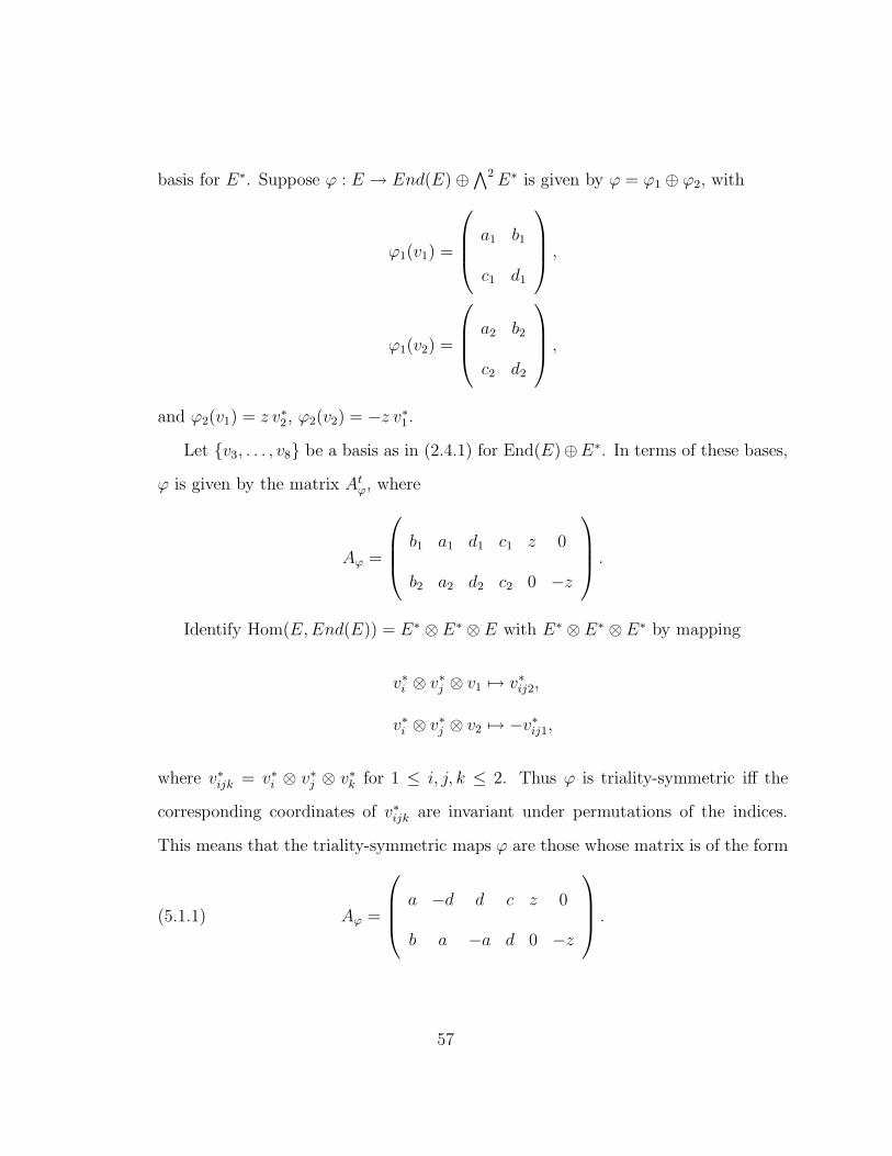
basis for E∗. Suppose ϕ : E → End(E) ⊕∧2 E∗ is given by ϕ = ϕ1 ⊕ ϕ2, with
ϕ1(v1) =
a1 b1
c1 d1
,
ϕ1(v2) =
a2 b2
c2 d2
,
and ϕ2(v1) = z v∗2, ϕ2(v2) = −z v∗
1.
Let v3, . . . , v8 be a basis as in (2.4.1) for End(E)⊕E∗. In terms of these bases,
ϕ is given by the matrix Atϕ, where
Aϕ =
b1 a1 d1 c1 z 0
b2 a2 d2 c2 0 −z
.
Identify Hom(E, End(E)) = E∗ ⊗ E∗ ⊗ E with E∗ ⊗ E∗ ⊗ E∗ by mapping
v∗i ⊗ v∗
j ⊗ v1 7→ v∗ij2,
v∗i ⊗ v∗
j ⊗ v2 7→ −v∗ij1,
where v∗ijk = v∗
i ⊗ v∗j ⊗ v∗
k for 1 ≤ i, j, k ≤ 2. Thus ϕ is triality-symmetric iff the
corresponding coordinates of v∗ijk are invariant under permutations of the indices.
This means that the triality-symmetric maps ϕ are those whose matrix is of the form
Aϕ =
a −d d c z 0
b a −a d 0 −z
.(5.1.1)
57

(Here a is also the coordinate of v∗122, b is the coordinate of v∗
222, −c is the coordinate
of v∗111, and −d is the coordinate of v∗
112.)
5.2. Orbits
In this section we compute the classes of orbit closures in the equivariant coho-
mology of a certain vector space; the connection with degeneracy loci is explained
in Appendix C. See [Fu5] for basic facts about equivariant cohomology. (For fields
other than C, one should use the equivariant Chow groups defined in [Ed-Gr2].)
Let G = G2 be the simple group of type G2, and fix a maximal torus T . Choose
simple roots α1 and α2, with α2 long. Let B be the corresponding Borel subgroup,
and let P = Pb2 be the maximal parabolic omitting α2. Let g, b, etc., denote the Lie
algebras, so p = b ⊕ g−α1 ⊂ g. Let P = L · Pu be the Levi decomposition, with Pu
the unipotent radical and L a Levi subgroup; L is isomorphic to GL2.
We will be interested in g/p as a P -module and as an L-module. As an L-module,
we have
g/p ∼=(Sym3 E∗ ⊗
∧2 E)⊕∧2 E∗,
where E ∼= C2 is the standard representation of L ∼= GL2 (normalized to have weights
α1 + α2 and 2α1 + α2). As a P -module, g/p does not split, but there is an exact
sequence
0 → Sym3 E∗ ⊗∧2 E → g/p →
∧2 E∗ → 0.
The T -weights of g/p are
−α2, −α1 − α2, −2α1 − α2, −3α1 − α2, −3α1 − 2α2.(5.2.1)
58

If we write t1 = −2α1 − α2 and t2 = −α1 − α2, the weights are
−t1 + 2t2, t2, t1, 2t1 − t2, t1 + t2.(5.2.2)
We wish to compute the classes of P -orbits in H∗T (g/p), so as a first step we give
explicit descriptions of these orbits.
By the classification given in [Ju-Ro], there are finitely many P -orbits on g/p. In
fact, there are five orbits. To describe them, let W = g/p and U = Sym3 E∗⊗∧2 E ⊂
W . Let b, a, d, c be coordinates on U , with weights −α2,−α1−α2,−2α1−α2,−3α1−
α2, respectively. The five orbits are Oc, with c = 0, 1, 2, 3, 5 giving the codimension;
their closures are nested and described by the following proposition:
Proposition 5.2.1. The P -orbit closures in W = g/p are as follows:
• O0 = W .
• O1 = U .
• O2 is the discriminant locus in U , defined by the vanishing of the quartic
polynomial a2d2 + 4a3c + 4bd3 − 27b2c2 + 18abcd.
• O3 is the (affine) cone over the twisted cubic curve in P3 = PU , defined by
the condition that the matrix
a −d c
b a d
have rank 1.
• O5 = O5 = 0.
Proof. The first claim is that W r U = O0 is a single dense orbit. This follows
from the classification of [Bu-He, Table 2].
59

It remains to verify the orbit decomposition of U . From the weights, we see that Pu
acts trivially on U , so the effective action is by P/Pu∼= GL2. Identify U with the space
of homogeneous cubic polynomials in two variables: U = −cx3−dx2y +axy2 + by3,
with GL2 acting so that the weights on a, b, c, d are as specified before the proposition.
We see that there are four orbits in U : the polynomials with distinct roots, those with
a double root, those with a triple root, and the zero polynomial. The given equations
for the closures of these loci are well known; see e.g., [La, IV, Ex. 12(b)] for the
discriminant and [Fu-Pr, §1.1] for the cubic curve. The proposition follows.
From the description in terms of cubic polynomials, it is easy to find represen-
tatives for orbits in U . Here we give representatives as weight vectors in g/p. Let
Yα ∈ g/p be a weight vector for α. We have
O0 = P · Y−3α1−2α2 = W r U ;
O1 = P · (Y−3α1−α2 + Y−α2)∼= P/Pu
∼= GL2;
O2 = P · Y−α1−α2 ;
O3 = P · Y−α2;
O5 = 0.
Using Proposition 5.2.1, it is a simple matter to compute the equivariant classes:
60

Theorem 5.2.2. In H∗T (W ) = Z[α1, α2] = Z[t1, t2], we have
[O0] = 1
[O1] = −3α1 − 2α2
= t1 + t2
[O2] = 2(−3α1 − 2α2)2
= 2(t1 + t2)2;
[O3] = −3(α1 + α2)(2α1 + α2)(3α1 + 2α2)
= 3t1t2(t1 + t2);
[O5] = −α2(α1 + α2)(2α1 + α2)(3α1 + α2)(3α1 + 2α2)
= t1t2(t1 + t2)(2t1 − t2)(−t1 + 2t2).
Proof. The normal space to U = O1 ⊂ W has weight −3α1−2α2, so the formula
for [O1] is clear. Since the restriction H∗T (W ) → H∗
T (U) is an isomorphism, the Gysin
pushforward H∗T (U) → H∗
T (W ) is multiplication by [U ]. Therefore it suffices to
compute the remaining classes in H∗T (U). The locus O2 is a hypersurface in U defined
by an equation of weight −6α1 − 4α2, so its class in H∗T (W ) is (−6α1 − 4α2) · [U ].
The class of [O3] in H∗T (U) is found by the classical Giambelli (or Salmon–Roberts)
formula. Finally, the class of the origin is the product of all the T -weights on W .
Remark 5.2.3. These classes cannot be computed by the “restriction equation”
method of Feher and Rimanyi [Fe-Ri2], because the stabilizer of O1 = P/Pu is
unipotent. This means the restriction map H∗P (W ) → H∗
P (O1) ∼= H∗Pu
(pt) = H∗(pt)
is zero in positive degees, and all the restriction equations are of the form 0 = 0. (The
problem persists for the other orbits.)
61

The formulas of Theorem 1.1.6 may be deduced from those of Theorem 5.2.2 using
the following lemma:
Lemma 5.2.4. The orbit
O3 ⊂ g/p ⊂ Hom(E, End(E) ⊕ E∗)
consists of the triality-symmetric morphisms of rank 1.
Proof. First note that any rank 1 map ϕ must correspond to an element ϕ1⊕ϕ2 ∈
W = U ⊕∧2 E∗ with ϕ2 = 0, i.e., ϕ lies in U . (If ϕ2 6= 0, then ϕ surjects onto E∗.)
Now the action of P on U is the same as that of its Levi subgroup GL2. The
inclusion P → Pb2 ⊂ GL8 induces an inclusion of Levi subgroups GL2 → GL2 ×GL6,
and the latter acts by conjugation on Hom(E, End(E)⊕E∗), so it preserves ranks of
morphisms. Therefore it will suffice to check that a representative for O2 has rank 2,
and a representative from O3 has rank 1. For these, we use the coordinate description
given in §5.1. Under the identification of U with the space of cubic polynomials, the
monomial xy2 corresponds to the basis vector v∗122. The orbit is O2 (since xy2 has
two distinct zeroes), and the corresponding matrix Aϕ has b = c = d = 0 and a 6= 0;
it is easy to see this means ϕ has rank 2. Similarly, x3 corresponds to v∗111, and the
corresponding Aϕ has a = b = d = 0 and c 6= 0, so ϕ has rank 1.
5.3. Graphs
For any morphism ϕ : E → F , let Eϕ ⊂ E ⊕ F be its graph, i.e., the subbundle
whose fiber over x is Eϕ(x) = (v, ϕ(v)) | v ∈ E(x). If ϕ : E → E∗ is symmetric,
then its graph is isotropic for the canonical skew-symmetric form on E ⊕E∗, defined
by (v1 ⊕ f1, v2 ⊕ f2) = f1(v2) − f2(v1). Thus one obtains a map to the Lagrangian
62

bundle of isotropic flags in E ⊕ E∗, and formulas for the degeneracy loci of ϕ are
deduced from formulas for Schubert loci; see [Fu3] or [Fu-Pr].
In this section, we consider morphisms ϕ : E → End(E) ⊕ E∗. By Proposition
2.4.1, there is a canonical octonion algebra structure on E ⊕ End(E) ⊕ E∗. We give
formulas for degeneracy loci of morphisms whose graphs are isotropic with respect to
this structure. In general such morphisms are not triality-symmetric (nor vice-versa).
For rank 1 maps, however, the two notions agree.
Lemma 5.3.1. Suppose X is a point, and ϕ : E → End(E) ⊕ E∗ is a triality-
symmetric map, with matrix Atϕ as in (5.1.1):
Aϕ =
a −d d c z 0
b a −a d 0 −z
.
Then the graph Eϕ is contained in V ⊂ C, and is γ-isotropic if and only if
a2 + bd = ac + d2 = ad − bc = 0.(5.3.1)
Proof. This is a straightforward verification, using the basis vi as in §5.1.
After a suitable change of coordinates (including a switch to opposite Schubert cells),
the parametrization of the open Schubert cell given in §D.1 becomes
Ωo =
1 0 a −d d c z −X
0 1 b a −a d −Z −Y
,(5.3.2)
where X = −ac − d2, Y = z + ad − bc, and Z = −a2 − bd. It is clear that the row
span is always in V ⊂ C, since the fourth and fifth columns add to zero. (In the
63

v-basis, V is defined by v∗4 + v∗
5 = 0.) The condition that the row span be the graph
Eϕ means X = Z = 0 and Y = z, which are precisely the equations (5.3.1).
Corollary 5.3.2. Let ϕ : E → End(E) ⊕ E∗ be a morphism of rank at most
1, and such that the component ϕ2 : E → E∗ is zero. Then ϕ is triality-symmetric
if and only if Eϕ ⊂ C is contained in V ⊂ C and γ-isotropic. (This holds scheme-
theoretically, i.e., the equations locally defining these two subsets of Hom(E, End(E))
are the same.)
Proof. This is a local statement, so we may assume X is a point and compute in
coordinates. In this case, it follows from Lemma 5.3.1 by adding the equation z = 0.
(The rank condition is forced by ϕ2 ≡ 0.)
Taking X to be a point, Corollary 5.3.2 says O3 = Ωo ∩ Ωtst. It follows that the
formulas for degeneracy of morphisms with γ-isotropic graphs are the same as those
of Theorem 1.1.6.
Theorem 5.3.3. Let ϕ : E → End(E)⊕E∗ be a morphism, and suppose its graph
Eϕ is γ-isotropic in V . If X is Cohen-Macaulay and Dr(ϕ) has expected codimension,
then [Dr(ϕ)] = Pr(c1, c2), where Pr is the polynomial of Theorem 1.1.6. Namely,
P2 = 1,
P1 = 3 c2 c1 = 3x1x2(x1 + x2),
P0 = c2 c1 (9 c2 − 2 c21) = x1x2(x1 + x2)(2x1 − x2)(−x1 + 2x2).
Proof. Let ϕ : E → End(E) ⊕ E∗ have γ-isotropic graph Eϕ. Suppose E has
a rank 1 subbundle, so Eϕ also does. Write E1 ⊂ E2 = E and F1 ⊂ F2 = Eϕ, and
extend these to complete γ-isotropic flags E• and F•, as in §1.1.2. Write Qi = V/F7−i.
64

For w ∈ W (G2), set
Ωw(ϕ) = x ∈ X | rk(Ep(x) → Qq(x)) ≤ rw(q, p), 1 ≤ p, q ≤ 7.
Since Eϕ∼= E, the Chern classes are the same. Let −x1,−x2 be Chern roots of E (so
x1, x2 are Chern roots of E∗). Then as in §1.1.5, we have
[Ωw(ϕ)] = Pw(x1, x2;−x1,−x2)(5.3.3)
in H∗X.
It remains to determine the w for which Dr(ϕ) = Ωw(ϕ). We have
Dr(ϕ) = x ∈ X | dim(E(x) ∩ Eϕ(x)) ≥ 2 − r
(cf. §C.2.1), and it is easy to check that
D2(ϕ) = Ωid(ϕ) = Ω1 2(ϕ) = X,
D1(ϕ) = Ωtst(ϕ) = Ω3 6(ϕ),
D0(ϕ) = Ωtstst(ϕ) = Ω6 7(ϕ).
Indeed, Q5 = V/F2, so we have dim(E2 ∩ F2) ≥ 1 iff rk(E2 → Q5) ≤ 1 = r3 6(2, 5).
The other two identities are clear.
Specializing the polynomials Pw given in §D.2 for these three w’s, we obtain the
desired formulas.
Remark 5.3.4. Up to sign, the twelve polynomials Pw(x1, x2;−x1,−x2) are also
the equivariant localizations σw|w0; see §D.3.
65

Remark 5.3.5. Lemma 5.3.1 can also be deduced from Proposition C.3.4 as fol-
lows. The representation g2 → so8 ⊂ gl8 realizes n− as 8 × 8 matrices of the form
M =
a b
−d a
d −a
c d
z 0
0 −z
−d −a a −b
−c d −d −a
,(5.3.4)
with 0’s in the blank blocks. (Here we are embedding so8 in gl8 using the basis vi,
so the bilinear form is given by (2.4.3).) One checks that the equations coming from
M2 = 0 are exactly those of (5.3.1).
66

CHAPTER 6
Characteristic two
The main results of this thesis continue to hold without restriction on the char-
acteristic of the ground field. In this chapter, we explain the modifications necessary
to include the case where char(k) = 2. Throughout, k denotes an algebraically closed
field of characteristic 2, except in Proposition 6.1.5, where k is arbitrary.
Most of the work to be done concerns the relationship between trilinear forms and
octonions discussed in Chapter 2. Once the definitions are adjusted and corresponding
facts about homogeneous spaces checked, the results of Chapters 3, 4, and 5 hold,
with the same proofs.
6.1. Forms and octonions
All of the facts about composition algebras quoted in §2.1 hold in arbitrary char-
acteristic; see [Sp-Ve, §§1–2].
Let V be a k-vector space of dimension 7. The definitions of compatible and
nondegenerate forms given in Definition 1.1.1 become trivial when char(k) = 2, so
an alternate definition is needed. Using Lemma 2.2.4, we saw that there is a basis
f1, . . . , f7 for V such that a nondegenerate trilinear form is given by (2.2.8); we will
take this as a definition in characteristic 2.
Definition 6.1.1. Fix a basis f1, . . . , f7 for V . Let γ0 :∧3 V → k be defined by
γ0 = f ∗147 + f ∗
246 + f ∗345 + f ∗
237 + f ∗156.(6.1.1)
67

An alternating trilinear form γ is nondegenerate if it is equivalent to γ0 (under the
action of GL(V )).
Fix a basis f1, . . . , f7 for V . Let γ0 be as above, and define a symmetric bilinear
form β0 by
β0(fp, f8−q) = δpq, for p 6= 4 or q 6= 4;
β0(f4, f4) = 0.
(6.1.2)
We also need to specify the norm. In general, a quadratic norm N on a vector space
W is called nonsingular if the corresponding quadric hypersurface Q(N) ⊂ P(W ) is
nonsingular. (When char(k) 6= 2, this is the same as requiring N to be nondegenerate,
i.e., the associated bilinear form β(u, v) = N(u + v)−N(u)−N(v) is nondegenerate;
in characteristic 2, however, this bilinear form is alternating, so it is always degenerate
if dim W is odd.) Using the basis fi for V , let N0 be the nonsingular norm
N0 = f ∗1 f ∗
7 + f ∗2 f ∗
6 + f ∗3 f ∗
5 + (f ∗4 )2,
so the associated bilinear form is β0. Note that β0 is degenerate, with radical spanned
by f4.
Definition 6.1.2. An alternating trilinear form γ and a nonsingular quadratic
norm N are compatible if the pair (γ, N) is equivalent to (γ0, N0). A symmetric
bilinear form β is compatible with γ if it is the bilinear form associated to a compatible
norm.
A subspace F ⊆ V is N -isotropic if the restriction N |F is identically zero; this
condition replaces β-isotropicity in characteristic 2. The definition of γ-isotropicity
is the same: when dim F ≥ 2, the subspace F ⊂ V is γ-isotropic if the induced map
68

F ⊗ F → V ∗ is zero; a one-dimensional subspace is γ-isotropic if it is N -isotropic for
a compatible norm N .
The analogue of Proposition 2.2.1 is the following:
Proposition 6.1.3. Given a compatible pair (γ, N) on V , there is an octonion
algebra C with norm N ′ such that V = e⊥ ⊂ C, with γ = γ′|V and N = N ′|V , where
γ′ is the trilinear form induced by multiplication on C.
Proof. Choose a basis fi so that the pair is (γ0, N0). Let E = 〈f1, f2〉, and let
C = E ⊕End(E)⊕E∗ be equipped with the canonical octonion structure, as in §2.4.
Let v1, . . . , v8 be the basis for C as in (2.4.1). Mapping
f1 7→ v1
f2 7→ v2
f3 7→ v3
f4 7→ v4 − v5
f5 7→ v6
f6 7→ v7
f7 7→ v8
embeds V in C. It is straightforward to check the statements about restriction of
forms, and that V = e⊥.
Remark 6.1.4. This construction clearly works for any ground field k. Note
that the subspace E ⊂ V is γ-isotropic, and as a subspace of C, u · v = 0 for all
u, v ∈ E. Moreover, the bilinear form β ′ associated to N ′ on C is nondegenerate, and
γ′(u, v, w) = β ′(uv, w) for all u, v, w ∈ C. When char(k) = 2, the basis element f4 in
V maps to e in C.
69

The above construction apparently depends on the choice of the γ-isotropic sub-
space E ⊂ V ; we shall see that this is not the case. The following is another version
of Proposition A.2.2, but here the ground field k is arbitrary.
Proposition 6.1.5. Let (γ, N) be a compatible pair on V , and let C be an octo-
nion algebra as in Proposition 6.1.3. Let G(γ, N) ⊆ GL(V ) be the subgroup preserving
γ and N . Then G(γ, N) = Aut(C). In particular, G(γ, N) is simple of type G2, and
GL(V ) has a dense orbit in∧3 V ∗.
Proof. Proposition 6.1.3 shows that Aut(C) ⊆ G(γ, N). On the other hand,
we claim that G(γ, N) is semisimple of rank 2; since Aut(C) is also such a group,
the proposition will follow. First, we may assume (γ, N) = (γ0, N0), as before. The
faithful G(γ0, N0)-representation V/〈f4〉 is irreducible, since it is irreducible as a rep-
resentation of the subgroup Aut(C) [Sp-Ve, Theorem 2.3.3]. It follows that G(γ0, N0)
is reductive [Sp, Ex. 2.4.15].
Let T ′ ⊂ GL(V ) be the maximal torus diagonal with respect to the basis fi, so
T ′ ∼= (k∗)7. The subgroup of T ′ preserving γ0 is T × µ3, where T ∼= (k∗)2 ⊂ (k∗)7 is
the two-dimensional torus
T = (z1, z2, z1z−12 , 1, z−1
1 z2, z−12 , z−1
1 ).
Requiring that the subgroup also preserve N leaves only T . Note that T is a regular
torus in GL(V ), i.e., the centralizer CGL(V )(T ) is equal to T ′. Therefore T is a maximal
torus in G(γ, N), so G(γ, N) has semisimple rank 2. To see G(γ, N) is semisimple,
note that it has trivial center. Indeed, the center must be a subgroup of T , but one
checks that T lies in Aut(C), so it is a maximal torus of the simple group Aut(C).
The last statement follows from a dimension count.
70

Remark 6.1.6. A classification of trilinear forms on a seven-dimensional vector
space over an arbitrary field is given in [Co-He]; the form γ0 is equivalent to the
one discussed in (3.9) of that article. The proof given there fails when char(k) = 2,
however, since the bilinear form associated to a norm is degenerate.
It follows that the construction of the composition algebra C is canonical:
Corollary 6.1.7. Let (γ, N) be a compatible pair on V . Suppose fi and f ′i
are two bases for V for which (γ, N) has the form (γ0, N0). Let E = 〈f1, f2〉 and
E ′ = 〈f ′1, f
′2〉, and let V → C and V → C ′ be the corresponding composition algebras.
Then there is a unique isomorphism C∼−→ C ′ making the diagram
C∼ - C ′
V⊂
-
⊃
commute.
The analogue of Lemma 2.2.3 holds:
Lemma 6.1.8. Let (γ, N) be compatible on V , defining a composition algebra C.
Then a subspace L ⊆ V is γ-isotropic iff uv = 0 for all u, v ∈ L. In particular, any
γ-isotropic subspace is also N-isotropic.
Proof. This is clear for one-dimensional subspaces, since by definition a one-
dimensional space 〈u〉 is γ-isotropic iff N(u) = 0, and N(u)e = uu = −u2 for u ∈ V .
So assume dim L > 1. Let β be the bilinear form associated to N , and let γ′ and β ′
be the extensions to C.
If L is C-isotropic, then for all u, v ∈ L, γ′(u, v, ·) = β ′(uv, ·) ≡ 0 on C, so
γ(u, v, ·) ≡ 0 on V , i.e., L is γ-isotropic.
71

Conversely, suppose L is γ-isotropic, and let u, v ∈ L. Then γ(u, v, w) = β(uv, w) =
0 for all w ∈ V , so uv ∈ V ⊥ = 〈e〉. For contradiction, suppose uv 6= 0. Replacing u
and v with scalar multiples, we may assume uv = e and N(u) = N(v) = 1. But then
v = u−1 = u = −u, since u ∈ V = e⊥. This contradicts the assumption dim L > 1,
so it follows that uv = 0.
The last statement comes from the fact that the norm is determined by N(u)e =
uu = −u2(= u2) for u ∈ V .
6.2. Forms and homogeneous spaces
Our next goal is to establish the analogue of Proposition 1.1.2. At the same time,
we will show that Proposition A.4.1 holds in characteristic 2.
Let Q ⊂ P(V ) be the quadric defined by N , let G ⊂ Gr(2, V ) be the subvari-
ety parametrizing 2-dimensional γ-isotropic subspaces, and let F lγ ⊂ Q × G be the
incidence variety, as before. Observe that Proposition A.4.1(a) holds; its proof is
independent of characteristic.
The analogue of Proposition 1.1.2 is the following:
Proposition 6.2.1. Let (γ, N) be compatible on V , defining a composition algebra
C. Let u ∈ V have norm 0. Then the subspace
Eu = v ∈ V | uv = 0
is three-dimensional and N-isotropic. Moreover, every two-dimensional C-isotropic
subspace of Eu contains u.
This follows from the analogues of Lemmas 2.2.8 and 2.2.9, whose proofs are the
same as before:
72

Lemma 6.2.2. If u ∈ V is a nonzero N-isotropic vector, then
Eu = v ∈ V | uv = 0
is a three-dimensional N-isotropic subspace.
Lemma 6.2.3. Let u ∈ V be a nonzero N-isotropic vector, and let v, w ∈ Eu be
such that u, v, w is a basis. Then vw = λu for some nonzero λ ∈ k.
Using Proposition 6.2.1, we have a rank 3 bundle S3 on Q, and F lγ is identified
with the P1-bundle P(S3/S1) → Q as before. The proof of the rest of Proposition
A.4.1 therefore goes through. It follows that G = Aut(C) acts transitively on the set
of 2-dimensional γ-isotropic subspaces of V .
73

APPENDIX A
Lie theory
In this appendix, we recall general facts about representation theory and homoge-
neous spaces for linear algebraic groups, and apply them show the above description
of the G2 flag variety agrees with the Lie-theoretic one. We do not know suitable ref-
erences for Propositions A.2.2, A.2.6, and A.4.1, so we give proofs. All the remaining
facts are standard, and can be found in e.g. [Fu-Ha], [Hu1], [Hu2], [Sp], [De].
Most of these facts hold in arbitrary characteristic, so unless indicated otherwise,
k is any algebraically closed field.
A.1. General facts
Let G be a simple linear algebraic group, fix a maximal torus and Borel subgroup
T ⊂ B ⊂ G, and let W = N(T )/T be the Weyl group. Let R, R+, R−, and ∆ be
the corresponding roots, positive roots, negative roots, and simple roots, respectively.
For α ∈ ∆, let sα ∈ W be the corresponding simple reflection, and let sα ∈ N(T ) be
a choice of lift. For a subset S ⊂ ∆, let PS be the parabolic subgroup generated by B
and sα |α ∈ S. (Such parabolic subgroups are called standard.) For P = PS, write
R+(P ) = R+(S) for the set of positive roots which lie outside the span of the simple
roots in S, and similarly for R−(P ). Also write ı = ∆ r si, so Pbı is the maximal
parabolic in which the ith simple root is omitted. (For example, SL5/Pb2∼= Gr(2, 5).)
If P = PS is (standard) parabolic, its unipotent radical Pu ⊂ P is the maximal
normal unipotent subgroup. A parabolic group admits a decomposition P = L · Pu
with L ⊂ P a reductive subgroup, called a Levi subgroup; L can be chosen (uniquely)
74

to contain T . Write g, b, t, p, pu, l for the corresponding Lie algebras, and write
g = t ⊕⊕
α∈R gα for the root space decomposition. Thus pu =⊕
α∈R+(P ) gα, and
p = l ⊕ pu. (We sometimes use n for pu.) The subgroup P− = w0Pw0 is the opposite
parabolic subgroup; its Lie algebra is p− = l ⊕ p−u , where p−
u =⊕
α∈R+(P ) g−α.
The irreducible representations of G are indexed by dominant weights; write Vλ
for the representation corresponding to the dominant weight λ. In characteristic
0, if pλ ∈ P(Vλ) is the point corresponding to a highest weight vector, then G · pλ
is the unique closed orbit, and is identified with G/PS(λ), where S(λ) is the set of
simple roots orthogonal to λ with respect to a W -invariant inner product. In positive
characteristic, G/PS(λ) can still be embedded in P(V ) for some representation with
highest weight λ, but V need not be irreducible. (See [Hu2, §31] for these facts about
representations in arbitrary characteristic.)
A.2. Representation theory of G2
The Dynkin diagram of type G2 is
1 2,
with corresponding simple roots α1 and α2. The full root system can be drawn as
follows:
α1
α4α3 α5α2
α6
The lattice of abstract weights is the same as the root lattice (cf. [Hu2, §A.9]);
it follows that up to isomorphism, there is only one simple group of type G2 (over
75

the algebraically closed field k). From now on, let G denote this group, and fix
T ⊂ B ⊂ G corresponding to the root data. By Proposition 2.1.2, G ∼= Aut(C),
where C is the unique octonion algebra over k. Let V = e⊥ ⊆ C be the imaginary
subspace.
The dominant Weyl chamber for this choice of positive roots is the cone spanned
by α4 and α6; denote these fundamental weights by ω1 and ω2, respectively. One
checks that V has highest weight ω1, and is irreducible for char(k) 6= 2, so V = Vω1
is the minimal irreducible representation, called the standard representation of G.1
The adjoint representation g has highest weight ω2. (This is irreducible if char(k) = 0,
but not if char(k) = 3.) Over any field, one has g ⊆∧2 V .
Let γ be the alternating trilinear form on V ⊂ C induced by the multiplication,
let f1, . . . , f7 be the standard γ-isotropic basis (2.2.6), and let E = 〈f1, f2〉 ⊂ V .
As we will see (Proposition A.4.1), the stabilizer of E in G is a maximal parabolic
Pb2, so we have GL(E) ⊂ Pb2 ⊂ G.
Proposition A.2.1. The subgroup GL(E) ⊂ Pb2 is the Levi subgroup containing
T .
Proof. From the root data, we see that the Levi factor of p2 is gl2. Indeed,
p2 = (t1 ⊕ t2 ⊕ gα1 ⊕ g−α1) ⊕ (p2)u,
with [gα1 , g−α1 ] = t1. Since GL(E) is a reductive subgroup with this Lie algebra,
containing T , the proposition follows.
From the description of G as the automorphisms of C, it is clear that G preserves
the alternating trilinear form γ. In fact, the converse is almost true:
1If char(k) = 2, the representation V = e⊥ ⊂ C contains an invariant subspace spanned by e. Inthis case, the irreducible representation Vω1
= V/(k · e) is 6-dimensional [Sp-Ve, §2.3].
76

Proposition A.2.2. Choose a basis f1, . . . , f7 for V , and let γ ∈∧3 V ∗ be
given by
γ = f ∗147 + f ∗
246 + f ∗345 − f ∗
156 − f ∗237,
as in (2.2.8). Let G(γ) ⊂ GL(V ) be the stabilizer of γ under the natural action, and
let SG(γ) = G(γ)∩SL(V ). Then SG(γ) is simple of type G2, and G(γ) = µ3×SG(γ).
Moreover, the orbit GL(V ) · γ is open in∧3 V ∗.
For k = C, this is well known; see [Br, §2] or [Fu-Ha, §22]. For arbitrary fields,
compare [As, (3.4)] and [Co-He, (2.1)]. We give a proof for char(k) 6= 2.
Proof. Fix an isomorphism ι :∧7 V ∗ ∼= k, and let βγ be as in (1.1.2). Since γ
and βγ are compatible, they define a composition algebra C (Proposition 2.2.1). Let
G = Aut(C); this is simple of type G2, and it is a subgroup of SL(V ) (Proposition
2.1.2).
Since γ may be recovered from the composition algebra structure as in (2.2.1),
we have G ⊆ SG(γ). On the other hand, SG(γ) preserves βγ, since it preserves ι.
Therefore it preserves the algebra structure on C, so SG(γ) = G.
The group of scalars Gm ⊂ GL(V ) acts on γ by λ · γ = λ−3γ, so Gm ∩G(γ) = µ3.
It follows that G(γ) = µ3 × SG(γ), so dim G(γ) = dim SG(γ) = 14.
Finally, the orbit GL(V ) · γ ⊂∧3 V ∗ is isomorphic to the homogeneous space
GL(V )/G(γ). Since dim GL(V )/G(γ) = 49 − 14 = 35 = dim∧3 V ∗, the orbit is
dense (and hence open).
The proof of this proposition also shows the following:
Corollary A.2.3. Let V , γ, and SG(γ) be as in Proposition A.2.2, and assume
char(k) 6= 2. Then SG(γ) acts irreducibly on V .
77

Proof. We have seen that SG(γ) = Aut(C) for a composition algebra such that
V = e⊥, and this is an irreducible representation.
Remark A.2.4. Consider the map ϕ : GL(V ) →∧3 V ∗, ϕ(g) = g · γ, and let dϕ :
gl(V ) →∧3 V ∗ be the differential. Let g(γ) = Lie(G(γ)) and sg(γ) = Lie(SG(γ)),
so g(γ) ⊆ ker dϕ, and sg(γ) ⊆ (sl(V ) ∩ ker(dϕ)). If char(k) 6= 3, a straightforward
computation shows that dϕ is surjective, so dim ker dϕ = 14. Proposition A.2.2 can
be proved using this (cf. [Fu-Ha, p. 357]). If char(k) = 3, dϕ is not surjective, but a
similar computation shows dim ker dϕ = 15, and dim(sl(V ) ∩ ker(dϕ)) = 14.
Remark A.2.5. Our proof that∧3 V ∗ has an open orbit relies on computations
with the specific form γ, and the apparently extraneous construction of a composition
algebra. There is a more conceptual reason for the existence of open orbits, as follows.
One shows that G2 stabilizes some vector in∧3 V ∗, and that G2 is not contained in
any parabolic subgroup of GL(V ). By a general theorem of Rohrle, stabilizers of
vectors in non-open orbits are always contained in parabolics.2 See [Ga3, §9.12] for
details and an application where the stabilizer is F4.
Note that w0 ∈ W acts on the weight lattice by multiplication by −1. This implies
that every irreducible representation of G is isomorphic to its dual. Using Schur’s
lemma, there is a unique (up to scalar) G-invariant bilinear form on each irreducible
representation [Hu2, §31.6]. In particular, we have the following:
Proposition A.2.6. Assume char(k) 6= 2. Let V be a 7-dimensional vector space,
with nondegenerate trilinear form γ :∧3 V → k. Then γ determines a compatible
form β uniquely up to scaling by a cube root of unity.
2If chark = 2, this argument fails: in that case, G2 has a faithful representation of degree 6, andGL6 lies in the Levi factor of a maximal parabolic of GL(V ).
78

Proof. Let G = SG(γ) ⊂ SL(V ) be the subgroup preserving γ. Then G is simple
of type G2 and acts irreducibly on V , so the discussion above shows there is a G-
invariant bilinear form β, unique up to scalar. Suppose β and λβ are compatible with
γ, for some λ ∈ k∗. If ϕ† ∈ V is the inverse image of ϕ under the isomorphism V → V ∗
determined by β, and ϕ‡ is the inverse image under the isomorphism determined by
λβ, then ϕ‡ = λ−1ϕ†. Thus we have
γ(u, v, γ(u, v, ·)‡) =1
2
(λβ(u, u) λβ(v, v)− (λβ(u, v))2
),
λ−1γ(u, v, γ(u, v, ·)†) =1
2λ2(β(u, u)β(v, v)− β(u, v)2
),
so λ3 = 1.
Remark A.2.7. In characteristic 0, the description of G2 (or g2) as the stabilizer
of a generic alternating trilinear form is due to Engel, who also found an invariant
symmetric bilinear form. For a history of some of the early constructions of G2, see
[Ag].
A.3. The Weyl group
The Weyl group of type G2 is the dihedral group with 12 elements. Let α1 and
α2 be the simple roots, with α2 the long root, and let s = sα1 and t = sα2 be the
corresponding simple reflections generating W = W (G2). Thus W has a presentation
〈s, t | s2 = t2 = (st)6 = 1〉. With the exception of w0, each element of W (G2) has a
unique reduced expression. The Hasse diagram for Bruhat order is as follows:
79

w0 = 7 6 (tststs = ststst)
(ststs) 7 5 6 7 (tstst)
(tsts) 6 3 5 7 (stst)
(sts) 5 2 3 6 (tst)
(ts) 3 1 2 5 (st)
(s) 2 1 1 3 (t)
id = 1 2
The indexing w = w1 w2, for 1 ≤ w1, w2 ≤ 7, arises as follows. There is an
embedding W (G2) → W (A6) = S7, given by s 7→ τ12τ35τ67 and t 7→ τ23τ56, where τij
is the permutation transposing i and j. (This also factors through W (B3).) Thus
each w is identified with a permutation w1 w2 · · ·w7, and in fact, the full permutation
is determined by w1 w2.
This inclusion of Weyl groups corresponds to the inclusion G2 → SL7 determined
by the basis f1, . . . , f7 for V = Vω1 and the trilinear form γ of (2.2.8), together with
the inclusion of tori (z1, z2) 7→ (z1, z2, z1z−12 , 1, z−1
1 z2, z−12 , z−1
1 ). Thus a natural way to
extend w ∈ W to a full permutation is as follows. Given w1 w2, let w3 be the number
such that Efw1= 〈fw1, fw2, fw3〉 as in §3.1.1. Then define w4, . . . , w7 by requiring
wi + w8−i = 8. For example, 6 3 extends to 6 3 7 4 1 5 2. Note that (w · w0)i = 8 − wi.
All this can be summarized in the following diagram:
1 2
3 4 5
6 7
1 2 2 11 3 2 5
3 1 5 2
3 6 5 7
6 3 7 56 7 7 6
st
80

A.4. Homogeneous spaces
We can now identify the homogeneous spaces for G2. In this section, we allow
k to have arbitrary characteristic. We take G = Aut(C) for an octonion algebra C,
as above, and let β and γ be the corresponding compatible forms on the imaginary
subspace V ⊂ C (replacing β with the norm N if char(k) = 2). From the root data,
one sees dim G = 14, dim B = 8, dim Pb1 = dim Pb2 = 9, and dim T = 2. Thus
dim G/B = 6 and dim G/Pb1 = dim G/Pb2 = 5.
Proposition A.4.1. Let F lγ, Q, and G be as in §3.1. Then
(a) Q ∼= G/Pb1,
(b) G ∼= G/Pb2, and
(c) F lγ ∼= G/B.
Proof. The homogeneous spaces G/Pb1 and G/Pb2 are the closed orbits in P(V )
and P(g), respectively. Since G preserves β (or N , in characteristic 2), G/Pb1 must be
contained in the quadric hypersurface Q ⊂ P(V ), but dim G/Pb1 = 5, so it is all of Q.
This proves (a).
For (b), note that G/Pb2 ⊂ P(g) ⊂ P(∧2 V ), so G/Pb2 ⊂ Gr(2, 7). Since G preserves
γ, we must have G/Pb2 ⊆ G; thus it will suffice to show G is irreducible and 5-
dimensional. For this, consider
F lγ = (p, ℓ) | p ∈ ℓ ⊂ Q × G,
and by Proposition 1.1.2 (which in turn used part (a)), the first projection identifies
F lγ with the P1-bundle P(S3/S1) → Q. Therefore F lγ is smooth and irreducible of
dimension 6. On the other hand, the second projection is obviously a P1-bundle.
81

Finally, since F lγ is a 6-dimensional G-invariant subvariety of G/Pb1 × G/Pb2, it
follows that F lγ = G/B, proving (c).
Remark A.4.2. A similar description of G/Pb2, among others, can be found in
[La-Ma].
We recall a few more facts for general G, P, B, T, W . The length of an element
w ∈ W is the least number ℓ = ℓ(w) such that w = s1 · · · sℓ (with sj = sαjfor some
αj ∈ ∆); such a minimal expression for w is called a reduced expression. Write
w0 for the (unique) longest element of W . The Bruhat order on W is defined by
setting v ≤ w if there are reduced expressions v = sβ1 · · · sβℓ(v)and w = sα1 · · · sαℓ(w)
such that the β’s are among the α’s.
For each w ∈ W , there is a Schubert cell Xow = BwB/B in G/B, of dimension
ℓ(w). The Schubert varieties Xw are the closures of cells, and Xv ⊆ Xw iff v ≤ w.
Let B− = w0Bw0 be the opposite Borel, and let N− ⊂ B− be its unipotent
radical. Then the map N− → w0 · Xow0
= B−B/B is an isomorphism, identifying
N− with a neighborhood of eB in G/B (cf. [Sp, (8.3.6)]). The same holds for P
a parabolic, with N− = P−u ⊂ P− the unipotent radical of the opposite parabolic
mapping isomorphically to the open set B−P/P ⊂ G/P .
Proposition A.4.3. Let i : G → G′ be an inclusion of semisimple algebraic
groups, and let B ⊂ G and B′ ⊂ G′ be Borel subgroups with i(B) ⊂ B′. Also
denote by i the induced inclusions of flag varieties G/B → G′/B′ and Weyl groups
W → W ′. Then for each w ∈ W , the Schubert cells are related by BwB/B =
(B′i(w)B′/B′) ∩ (G/B).
82

More generally, let P ⊂ G and P ′ ⊂ G′ be parabolic subgroups such that P =
P ′ ∩ G. Then the same conclusion holds for G/P → G′/P ′, that is, BwP/P =
(B′i(w)P ′/P ′) ∩ (G/P ) for all w ∈ W .
Proof. The inclusion BwB/B ⊆ (B′i(w)B′/B′) ∩ (G/B) is clear. For the other
direction, since the map i is B-equivariant, it is enough to note that the RHS is
B-stable and contains only one T -fixed point (namely wB).
The proof for G/P is exactly the same, mutatis mutandis.
A.5. The Borel map and divided differences
Let M ⊂ t∗ be the weight lattice. For general G/B, there is a Borel map
c : Sym∗ M → H∗(G/B)
induced by the Chern class map c1 : M → H2(G/B), where M ⊂ t∗ is the weight
lattice. More precisely, this map is defined as follows. Identify M with the character
group of B, and associate to χ ∈ M the line bundle Lχ = G ×B C. Then c1(χ)
is defined to be c1(Lχ). (See [BGG, De].) In fact, c1 is an isomorphism, and this
induces an action of W in the evident way: for w ∈ W and x = c1(χ) ∈ H2(G/B),
define w · x = c1(w · χ).
The Borel map becomes surjective after extending scalars to Q, and sets up an
isomorphism
H∗(G/B, Q) ∼= Sym∗ MQ/I,
where I = (Sym∗ MQ)W+ is the ideal of positive-degree Weyl group invariants.
83

For a simple root α, define the divided difference operator ∂α on H∗(G/B) by
∂α(f) =f − sα · f
α.(A.5.1)
These act on Schubert classes as follows [De]:
∂α[Ωw] =
[Ωw sα] when ℓ(w sα) < ℓ(w);
0 when ℓ(w sα) > ℓ(w).
(A.5.2)
In particular, [Ωsα] can be identified with the weight at the intersection of the hyper-
planes orthogonal to α and the (affine) hyperplane bisecting α.
In the case of G2 flags, we know [Ωs] = x1 and [Ωt] = x1 +x2. Looking at the root
diagram, then, we see x1 = α4 and x2 = α3. Therefore
α1 = x1 − x2;
α2 = −x1 + 2x2;
s · x1 = x2;
s · x2 = x1;
t · x1 = x1;
t · x2 = x1 − x2.
With these substitutions, the operators of (A.5.1) agree with those defined in §4.1
((1.1.4) and (1.1.5)).
Remark A.5.1. The divided difference operators satisfy the braid relations defin-
ing W . (The algebra of divided differences is a representation of the nil-Hecke algebra.)
Thus if (α1, . . . , αℓ) is a reduced word for w, one can define ∂w = ∂α1 · · · ∂αℓ, and
84

this is independent of the choice of word. It follows from (A.5.2) that for any class
τ ∈ H2ℓ(G/B),
τ =∑
ℓ(w)=ℓ
(∂w(τ)) · [Ωw].
In principle, this can be used to compute any given product in the cohomology of a
flag variety; in practice, it is prohibitively inefficient. However, the G2 flag variety is
small enough to be treated by this brute-force method, which is how the computations
in Remark 4.2.2 were carried out.
A.6. Equivariant vector bundles
Proposition A.6.1. Let H ⊆ G be a closed subgroup, and let U be an H-module.
Then the functor
U 7→ G ×H U,
with the evident action on morphisms, is an equivalence between the category of H-
modules and the category of G-equivariant vector bundles on G/H. The functor taking
an equivariant vector bundle to its fiber at eH ∈ G/H is an inverse.
Using this, we deduce some basic facts about vector bundles on G = G/P , for
P = Pb2.
Corollary A.6.2. The tautological rank 2 subbundle S ⊂ V on G is the equi-
variant bundle
S = G ×P E,
85

where E is the 2-dimensional representation of P corresponding to the standard rep-
resentation of the Levi subgroup L ∼= GL(E) ⊂ P .
Proof. By definition, the fiber of S over eP = [E] ∈ G is E, and P stabilizes E.
We saw in Proposition A.2.1 that GL(E) is a Levi subgroup of P .
Corollary A.6.3. Let S ⊂ V be the tautological rank 2 subbundle on G, and let
i : G → Grβ′(2, C) be the inclusion. Then the tangent bundles are described by the
diagram below:
TG ⊂ - i∗TGrβ′
‖ ‖(Sym3 S∗ ⊗OG(−1)
)⊕OG(1) ⊂- Hom(S, End(S)) ⊕OG(1),
where OG(1) =∧2 S∗.
Proof. Restrict to fibers over [E] ∈ G, and use Proposition B.4.1.
86

APPENDIX B
Triality
If G is a simply-connected, split, semisimple group, then symmetries of the corre-
sponding Dynkin diagram induce the outer automorphisms of G (see, e.g., [Fu-Ha,
Prop. D.40] or [KMRT, §25.B]). The Dynkin diagram of type D4 possesses a symme-
try not shared by other Dynkin diagrams: the order 3 symmetry rotating the outer
nodes. The resulting symmetry of Spin8 is called triality.
Triality has a long and interesting history. In 1925, Cartan described the S3 ac-
tion on the root system of type D4 and its relationship to a geometric principe de
trialite, an incidence-preserving correspondence between points on a six-dimensional
quadric and each of the two families of P3’s in the quadric [Ca]. (This geometric cor-
respondence was also considered by Study in 1913.) Cartan also noted the connection
with automorphisms of the octonions, and the fact that the fixed subalgebra for the
corresponding action on so8 is g2. Since then, triality has been considered in several
contexts by many mathematicians. For example, Freudenthal used triality to unify
his construction of the exceptional Lie algebras; Springer and van der Blij clarified
some of Cartan’s remarks and gave formulations of triality valid over arbitrary fields;
and triality plays a central role in the classification of forms of D4 given in [KMRT].
In this chapter, we give a brief exposition of the manifestations of triality rele-
vant to the symmetries of morphisms described in Chapter 5. We make no claims
of originality: most of the ideas can be found in Cartan (without proofs). Other
87

references for this material include [vdB-Sp], [Sp-Ve, §3], [Ga1], [Fu-Ha, §20.3],
and [KMRT].
Throughout, k is an algebraically closed field of characteristic not 2.
B.1. D4 flags
Let C be an 8-dimensional k-vector space, equipped with a nondegenerate sym-
metric bilinear form β ′.1 Here we describe the variety of isotropic flags in C, generally
using the projective terminology: thus a point is a one-dimensional subspace of C,
a line is a two-dimensional subspace, etc. Let Q ⊂ P(C) = P7 be the 6-dimensional
quadric defined by β ′, and let Q2 = Grβ′(2, C) be the 9-dimensional Grassmannian of
(projective) lines in Q. Recall that there are two families of isotropic 4-dimensional
subspaces of C (i.e., spaces in Q); let Q+ = Gr+β′(4, 8) and Q− = Gr−β′(4, 8) be
these two families. (If one fixes a given space Σ+0∼= P3 ⊂ Q, then Q+ parametrizes
spaces Σ+ such that dim(Σ+∩Σ0) is odd, while Q− parametrizes spaces Σ− such that
dim(Σ− ∩ Σ0) is even.)
The D4 flag variety is the incidence variety
F lβ′(C) = (p, ℓ, Σ+, Σ−) | p ∈ ℓ ⊂ Σ+ ∩ Σ− ⊂ Q × Q2 × Q+ × Q−.
This is a homogeneous projective variety of dimension 12. The parity condition
implies that for any (Σ+, Σ−) ∈ Q+ × Q−, the intersection Σ+ ∩ Σ− is either a point
or a plane. For (p, ℓ, Σ+, Σ−) ∈ F lβ′ , we have dim(Σ+∩Σ−) = 2, since the intersection
contains the line ℓ. Thus a D4 flag also determines a plane, and there is a tautological
1Our notation is chosen to agree with that of earlier chapters, and in anticipation of §B.2, where wewill equip C with the structure of an octonion algebra.
88

flag of vector bundles
S+4
S1⊂ - S2
⊂ - S3
⊂
-
S5⊂ -
⊂
-
S6⊂ - S7
⊂ - C ,
S−4
⊂
-⊂
-
where Si = S⊥8−i.
Remark B.1.1. From this construction, we see that there are two embeddings
ι+, ι− : F lβ′(C) → F l(C) into the full flag variety, given by taking the middle flag
to be S+4 or S−
4 , respectively. (This is also equivalent to the choice of Σ0.) There is
an involution on F l(C) ∼= SL8/B defined by (E•) 7→ (E⊥8−•); the fixed locus has two
connected components, corresponding to these two embeddings.
Let pr134 : F lβ′ → Q × Q+ × Q− and pr2 : F lβ′ → Q2 be the projections, and let
Y ⊂ Q × Q+ × Q− be
Y = pr134(F lβ′) = (p, Σ+, Σ−) | dim(Σ+ ∩ Σ−) = 2 and p ∈ Σ+ ∩ Σ−.
The projection pr134 realizes F lβ′ as the P1 bundle P(S3/S1) → Y . The projection
pr2 realizes F lβ′ as a P1 × P1 × P1-bundle over Q2: Indeed, we have
F lβ′ = P(S2) ×Q2 Q(S6/S2),
where S2 is the tautological bundle on Q2, S6 = S⊥2 , and Q(S6/S2) is the quadric
bundle defined by the restriction of β ′. (The fibers are quadric surfaces in P3, so
isomorphic to P1 × P1.)
89

B.2. Geometric triality
The data parametrized by F lβ′(C) can be arranged suggestively on the D4 Dynkin
diagram as below.
p ℓ
Σ+
Σ−
The triality automorphism τ : F lβ′(C) → F lβ′(C) rotates this diagram; it also induces
automorphisms of Q2 and Y ⊂ Q×Q+×Q−. To describe it, we use some facts about
octonions.
Equip C with a split octonion algebra structure, with norm N corresponding to
the bilinear form β ′. (Recall that split means the norm is isotropic, i.e., there exist
nonzero vectors of norm 0.) This can be done as follows. Choose a vector e ∈ C of
norm 1 to serve as the identity. Then choose a basis f1, . . . , f7 for V = e⊥ such that the
restriction β = β ′|V has the form (2.2.7), and define multiplication using the trilinear
form γ of (2.2.8). Recall that conjugation is defined on C by u = β ′(u, e) e − u.
Lemma B.2.1 ([vdB-Sp, §2]). Let u ∈ C be a nonzero vector with N(u) = 0.
Then uC and Cu are 4-dimensional isotropic subspaces in different families. Con-
versely, every maximal isotropic subspace occurs this way, and the vector defining it
is unique up to scalar.
Now we can define maps Q2 → Q2, Q → Q+, Q+ → Q−, and Q− → Q (all
denoted by τ) as follows.
[u] [u, u′]
[vC]
[Cw]
τ−→
[w] [uC ∩ u′C]
[uC]
[Cv]
90

The fact that incidence is preserved under this map is what Cartan calls the principle
of triality ; see also [vdB-Sp, Theorem 7].
It is easy to check that τ 3 is the identity, so τ gives an action of Z/3Z on F lβ′(C).
Together with the involution induced by C → C, u 7→ u, this defines an action of the
symmetric group S3. We shall focus on the Z/3Z-action.
Let V ⊂ C be the 7-dimensional subspace of imaginary octonions, i.e., V = e⊥.
Let γ be the restriction to V of the trilinear form defined by multiplication on C;
recall that γ is an alternating form, and the G2 flag variety is the variety of γ-isotropic
flags in V (see §1.1.2). The following proposition is essentially well known, but the
proof we give sheds some light on the tautological rank 3 bundle on F lγ(V ).
Proposition B.2.2. The fixed locus F lβ′(C)τ for the Z/3Z action is the G2 flag
variety F lγ(V ). Similarly, the fixed locus for the action on Q2 = Grβ′(2, C) is the G2
Grassmannian G.
Proof. First consider the action on Y . The point ([u], [vC], [Cw]) ∈ Y ⊂ Q ×
Q+ ×Q− is fixed when [u] = [w] = [v] (and in this case the component [u] determines
the components [vC] and [Cw]). Now for [u] ∈ [uC], we must have u ∈ V . Indeed,
suppose u = ux for some x in C. Then u2 = u(ux) = (uu)x = N(u)x = 0. By the
minimal equation for u (see (2.1.1)), this implies β(u, e) = 0, i.e., u ∈ V . It follows
that the fixed locus Y τ is isomorphic to the 5-dimensional quadric Q ⊂ P(V ).
Next consider the action on Q2. A line [u, u′] is fixed by τ when [u, u′] = [uC∩u′C].
This is equivalent to the four conditions
u ∈ uC, u′ ∈ u′C, u ∈ u′C, u′ ∈ uC.
As discussed in the previous paragraph, the first two conditions are equivalent to
u, u′ ∈ V ⊂ C. The second two are equivalent to uu′ = 0: If u′ = ux for some x, then
91

uu′ = u(ux) = (uu)x = 0. Conversely, the kernel of the map x 7→ ux is precisely uC.
(The condition u ∈ u′C is verified similarly.) Now by Lemma 2.2.3, a τ -fixed line is
the same as a γ-isotropic line, i.e., a point of G = G2/P2.
Finally, since incidence is preserved by τ , the proposition follows.
Remark B.2.3. The variety Y comes with three tautological subbundles of the
trivial bundle C: S1, S+4 , and S−
4 , as well as the rank 3 bundle S3 = S+4 ∩ S−
4 . In the
above proof, we saw that the restriction of S1 to Y τ ∼= Q is a subbundle of V ⊂ C. A
symmetric argument shows that S3 ⊂ V ; this is precisely the rank 3 bundle described
in Proposition 1.1.2.
B.3. Root systems
The geometric triality described above comes from an automorphism of the simply
connected type-D4 group Spin8 which fixes the type G2 subgroup G = Aut(C). (See
[Sp-Ve, §3] for the details on this action and the “local triality” action on the corre-
sponding Lie algebras.) This automorphism of Spin8 is induced by an automorphism
of the D4 root system, which we now describe.2
Let T ′ ⊂ Spin8 be a maximal torus, with Lie algebra t′. The root system of
type D4 has 24 roots: R = ±t′i ± t′j : 1 ≤ i < j ≤ 4, where t′1, t′2, t
′3, t
′4 is an
orthonormal basis for t′∗ (with respect to a form invariant under the Weyl group).
Choosing simple roots
α′1 = t′1 − t′2, α′
2 = t′2 − t′3, α′3 = t′3 − t′4, α′
4 = t′3 + t′4,
2We shall not use any spin representations explicitly, and the reader more comfortable with orthog-onal groups may read Spin8 as SO8. However, it is important to remember that the Z/3Z actionsdescribed in this chapter lift only to Spin8 (or PSO8), and not to SO8.
92

the positive roots are R+ = t′i ± t′j | i < j. Label the D4 Dynkin diagram as follows,
with node i corresponding to the simple root α′i:
1 2
3
4
The triality action on t′∗ is given by
τ : α′1 7→ α′
4 7→ α′3 7→ α′
1,
τ : α′2 7→ α′
2.
In the t′-basis, τ has matrix
12
12
12
−12
12
12
−12
12
12
−12
12
12
12
−12
−12
−12
.
Note that at′1 + bt′2 + ct′3 + dt′4 is invariant under τ iff d = 0 and a = b + c, i.e.,
the invariant vectors are
b(t′1 + t′2) + c(t′1 + t′3).
The fixed positive roots are
t′2 − t′3 = α′2,
t′1 + t′3 = α′1 + α′
2 + α′3 + α′
4,
t′1 + t′2 = α′1 + 2 α′
2 + α′3 + α′
4.
93

Now let T ⊂ T ′ be a maximal torus of G = G2 = Aut(C), so T is fixed by τ ; let
t be its Lie algebra. Let α1 = t1 − t2 and α2 = −t1 + 2t2 be the simple roots, as in
§A.2. The restriction map t′∗ → t∗ is given by t′1 7→ t1, t′2 7→ t2, t′3 7→ t1 − t2, t′4 7→ 0.
In terms of the simple roots, this is
α′1, α
′3, α
′4 7→ α1;
α′2 7→ α2.
To see this, it is easiest to use the basis v1, . . . , v8 for C, as in (2.4.1). In this
basis, T ′ acts with weights t′1, t′2, t
′3, t
′4,−t′4,−t′3,−t′2,−t′1, while T acts with weights
t1, t2, t1 − t2, 0, 0, t2 − t1,−t2,−t1.
B.4. Tangent spaces
Let i : G → Grβ′(2, C) be the inclusion of the fixed locus for τ . Still using the
basis vi for C, let [E] ∈ Gr(2, C) be the point corresponding to E = 〈v1, v2〉. We
wish to compare the tangent spaces T[E]G and T[E]Grβ′ , both considered as subspaces
of T[E]Gr(2, C) = Hom(E, C/E).
Identify G = G/P and Grβ′ = Spin8/P′, for G = Aut(C), and P ⊂ G, P ′ ⊂ Spin8
maximal parabolic subgroups. Since [E] corresponds to the point eP ∈ G/P and
eP ′ ∈ Spin8/P′, we are considering
g/p ⊂ so8/p′ ⊂ Hom(E, C/E).
Moreover, τ acts on T[E]Grβ′ = so8/p′, fixing the subspace T[E]G = g/p. Recall that
GL(E) is a Levi subgroup of P ⊂ G.
94

Proposition B.4.1. As GL(E)-modules, the tangent spaces are described by the
diagram below:
T[E]G ⊂ - T[E]Grβ′
‖ ‖(Sym3 E∗ ⊗
∧2 E)⊕∧2 E∗ ⊂- Hom(E, End(E)) ⊕
∧2 E∗.
Proof. Representations of GL(E) ∼= GL2 are determined by their weights. The
weights of T ′ acting on T[E]Grβ′ = so8/p′ are the 9 roots
−α′2, −α′
1 − α′2, −α′
2 − α′3,
−α′2 − α′
4, −α′1 − α′
2 − α′3, −α′
1 − α′2 − α′
4,
−α′2 − α′
3 − α′4, −α′
1 − α′2 − α′
3 − α′4, −α′
1 − 2α′2 − α′
3 − α′4.
Restricting these to T -weights, we find the weights of so8/p′ are
−α2 = t1 − 2t2 (once)
−α1 − α2 = −t2 (three times)
−2α1 − α2 = −t1 (three times)
−3α1 − α2 = −2t1 + t2 (once)
−3α1 − 2α2 = −t1 − t2 (once),
which agree with those of Hom(E, End(E)) ⊕∧2 E∗.
A similar calculation verifies g/p ∼= Sym3 E∗ ⊗∧2 E ⊕
∧2 E∗, and also that the
normal space (so8/p′)/(g/p) has weights
−α1 − α2 = −t2 (twice)
−2α1 − α2 = −t1 (twice),
95

and hence is isomorphic to E∗ ⊕ E∗ as a GL(E)-module.
96

APPENDIX C
Graphs and symmetry
Let ϕ : E → F be a morphism of vector bundles on a variety. There are at least
two ways of defining symmetry for such a morphism, with corresponding methods for
producing degeneracy loci. The purpose of this appendix is to describe the relation-
ship between these two methods, and to introduce appropriate generalizations. The
essential ingredient is a comparison of the exponential map for Lie algebras with the
graph map for morphisms.
C.1. The exponential map
In this section, we assume the ground field is C (but see Remark C.1.3). There is
an analytic map exp : gln → GLn given by
exp(X) = 1 + X +1
2X2 +
1
6X3 + · · · .(C.1.1)
The same formula defines an exponential map exp : g → G for any subgroup G ⊂ GLn
with Lie algebra g.
When N ⊂ GLn is unipotent, so its Lie algebra n is nilpotent, the map exp : n →
N is algebraic. In fact, this is an isomorphism of algebraic varieties, defined over
Z[ 1n!
].
We shall first consider a special case. Recalling the notation of §A.1, let P bm ⊂ GLn
be a (standard) maximal parabolic, so GLn/P bm = Gr(m, n). Let N−bm be the unipotent
radical of the opposite parabolic. Let pm and n−m be the Lie algebras, so gln = n−
m⊕pm.
97

Then X2 = 0 for all X ∈ n−m, so (C.1.1) reduces to exp(X) = 1 + X; in particular,
exp : n−m → N−
m is defined over Z.
Let E be the subspace spanned by the first m standard basis vectors for V = Cn,
so it corresponds to the point [E] = eP bm in GLn/P bm. Let F be the subspace spanned
by the last n − m basis vectors. Then n−m is canonically isomorphic to Hom(E, F ),
as can be seen from the block forms of pm and n−m (using the standard basis to
identify gln with n×n matrices). Write Ωo = N−bm ·P bm/P bm for the open neighborhood
of [E] parametrizing subspaces which map surjectively to E under the projection
V = E ⊕ F → E; as in §A.4, we have N−bm∼= Ωo via the map x 7→ x · eP bm.
For ϕ ∈ Hom(E, F ), let Eϕ ⊂ E ⊕ F be the graph of ϕ, i.e., the subspace
(v, ϕ(v)) | v ∈ E. Thus there is an injective graph morphism gr : Hom(E, F ) →
Gr(m, n) given by gr(ϕ) = [Eϕ].
Proposition C.1.1. Under the identifications n−m = Hom(E, F ) and N−
bm = Ωo,
the map exp : n−m → N−
bm is identified with the graph morphism gr : Hom(E, F ) →
Gr(m, n).
Proof. Using the standard basis, the map exp is given in terms of matrices by
0m 0
∗ 0n−m
7→
Im 0
∗ In−m
,
where Im is the m×m identity matrix, 0m is the zero matrix, and ∗ is an (n−m)×m
matrix corresponding to an element ϕ ∈ Hom(E, F ). The first m columns of the
n × n matrix on the RHS span Eϕ.
Now let G ⊂ GLn be a semisimple (or reductive) subgroup such that P = P bm ∩G
is parabolic in G, so the inclusion induces i : G/P → Gr(m, n). Let N− be the
98

unipotent radical of the opposite parabolic of P . Let g, p, n− be the Lie algebras,
considered also as subalgebras of gln. In general, n− is not contained in n−m. (Indeed,
this happens exactly when P bm is the smallest parabolic subgroup of GLn containing
P .) However, there is a natural inclusion g/p → gln/pm, so one obtains an inclusion
ı : n− → n−m via an isomorphism n− ∼= g/p.
Write ΩoG = N− · P/P ⊂ G/P , and identify this with N− as before. Thus the
exponential map gives an inclusion exp : n− ∼−→ N− = Ωo
G ⊂ Ωo ⊂ Gr(m, n).
Proposition C.1.2. Let gr : Hom(E, F ) → Gr(m, n) be the graph map, and let
Z ⊆ n− be the subscheme defined by
Z = X ∈ n− |X2 = 0,(C.1.2)
where “X2” is defined via the given representation n− ⊂ g ⊂ gln. Then Z =
gr−1(ΩoG) ∩ ı(n−). In other words, the diagram
Z ⊂ - n−
n−?
∩
⊂exp- Gr(m, n)
gr ı?
∩
is cartesian.
Proof. We want to show exp(X) = gr ı(X) iff X ∈ Z. Let ν be the smallest
integer such that Xν+1 = 0 for all X ∈ n−. Then exp(X) = 1+X + 12X2 + · · ·+ 1
ν!Xν
and gr ı(X) = 1 + X, so it is clear that Z ⊆ gr−1(ΩoG) ∩ ı(n−).
On the other hand, suppose exp(X) = gr ı(X), i.e.,
1
2X2 + · · ·+
1
ν!Xν = 0.(C.1.3)
99

Since the nonzero powers of a nilpotent element are linearly independent, (C.1.3)
implies X2 = 0.
Remark C.1.3. The restriction on the characteristic of the ground field is not
strictly necessary. The scheme Z of (C.1.2) is defined over Z, as is exp |Z . The first
paragraph of the proof thus shows Z ⊆ gr−1(ΩoG) ∩ ı(n−) over any field.
C.2. Two methods
We illustrate two methods for finding formulas for degeneracy loci for a morphism
ϕ : E → F , in the case of a symmetric morphism, so F = E∗ and ϕ = ϕ∗ : E → E∗.
Let E have rank m.
C.2.1. Schubert loci in bundles. In the first method, one constructs an aux-
iliary vector bundle V = E ⊕ E∗, with a symplectic form ω; specifically, ω(x1 ⊕
f1, x2 ⊕ f2) = f1(x2) − f2(x1). In other words, V comes with a canonical reduc-
tion of structure group from GL2m to Sp2m. The subbundle E = E ⊕ 0 ⊂ V is
clearly isotropic, and the morphism ϕ is symmetric iff its graph Eϕ is isotropic in V .
Moreover, ker(ϕ) = E ∩ Eϕ, so we have an identification
Dr(ϕ) = Ωm−r := x ∈ X | dim(E(x) ∩ Eϕ(x)) ≥ m − r.
There is an associated Grassmann bundle
LG(V )π−→ X,
whose fiber over x is the Lagrangian Grassmannian of isotropic m-planes in V (x).
Let S ⊂ V be the tautological rank m subbundle on LG(V ), and let E ⊂ V also
100

denote the bundles pulled back to LG(V ). In LG(V ), there are Schubert loci
Ωp = Ωp(E, S) = x ∈ LG(V ) | dim(E(x) ∩ S(x)) ≥ p
The bundle LG(V ) → X has sections sE and sϕ corresponding to the isotropic
subbundles E and Eϕ, and one sees that Dr(ϕ) = s−1ϕ (Ωm−r):
Ωm−r⊂ - LG(V )
Dr(ϕ)
6
⊂ - X.
sϕ6
Thus the problem is reduced to computing formulas for Schubert loci in H∗LG(V ).
This can be done by first finding a formula for the most degenerate locus, Ωm =
x |E(x) = S(x), and then applying divided difference operators to deduce formulas
for the others.
This is essentially the method used by Fulton in [Fu2] and [Fu3] (see also [Fu-Pr]).
An advantage of this approach is that it works for all flag bundles, and the machinery
of divided difference operators reduces the problem (in principle) to that of computing
a single class for each case.
C.2.2. Orbits. An alternative approach is to work with the space of symmetric
morphisms more directly. Continuing with the example of a symmetric morphism
ϕ : E → E∗, one proceeds as follows. Note that ϕ corresponds to a section sϕ of
the vector bundle Sym2 E∗ → X. Inside this vector bundle there is a locus Dr of
morphisms with rank at most r; we are looking for the locus where sϕ meets Dr:
Dr⊂ - Sym2 E∗
Dr(ϕ)
6
⊂ - X.
sϕ
6
101

It suffices to solve this on the classifying space for E, so take X = BGLm. Then
Sym2 E∗ is the vector bundle corresponding to the representation Sym2(Cm)∗ of GLm.
This representation has finitely many GLm-orbits Or, for 0 ≤ r ≤ m, corresponding
to the symmetric matrices of rank r. Let Dr = Or be the locus of matrices of rank
at most r, so we have
Dr = EGLm ×GLm Dr ⊆ EGLm ×GLm Sym2(Cm)∗ = Sym2 E∗
over BGLm. (Here EGLm → BGLm is the universal principal GLm-bundle.)
Computing the class [Dr(ϕ)] ∈ H∗X thus reduces to computing the equivari-
ant class of an orbit closure in a vector space: we want a formula for [Dr]G ∈
H∗G(Sym2(Cm)∗) = H∗
G(pt). This is essentially the method used by Harris and Tu
[Ha-Tu] (without the language of equivariant cohomology), and developed further
by Feher, Nemethi, and Rimanyi [Fe-Ne-Ri]; see also [Fe-Ri2].
This method has the advantage of producing manifestly unique formulas: the
equivariant cohomology ring H∗G(pt) is frequently a polynomial ring. (In fact, it will
be a polynomial ring for the cases we study.) Also, it is often an easy matter to
determine the most degenerate class [D0]G. Using an embedding H∗
G(pt) ⊂ H∗T (pt),
for T a maximal torus, the orbit D0 = 0 has class equal to the product of the
T -weights of the representation. On the other hand, it is less clear what the action
of divided difference operators means in this context; they may not produce formulas
for orbit closures.
C.3. General setup
Here we introduce two general notions of symmetry for morphisms correspond-
ing to the two methods, called “G/P symmetry” and “g/p symmetry,” respectively.
102

The example discussed above will correspond to the case G = Sp2m, with maximal
parabolic P = P bm, so G/P = LG(2m); the two notions coincide in this case.
Given a map of vector bundles ϕ : Em → Fn−m on X, let V = E ⊕ F , so V has
rank n. From this data, we obtain a (not commutative!) diagram:
Hom(E, F )
X
sϕ6
sE
- Gr(m, V ).
gr⊂
-
Here sϕ and sE are the sections determined by ϕ : E → F and E ⊂ V , respec-
tively, and gr is the graph morphism, defined locally as in §C.1.1 Injectivity
is easily checked on fibers: for a point x ∈ X, gr(x) gives an isomophism from
Hom(E(x), F (x)) onto the open Schubert cell in Gr(m, V (x)) consisting of subspaces
projecting isomorphically to E(x). Note that gr sϕ = sEϕis the section correspond-
ing to the graph of ϕ.
Since Hom(S, Q) is the relative tangent bundle to Gr(m, V ) → X, we see that
Hom(E, F ) = s∗EHom(S, Q) is the normal bundle to sE(X) ⊂ Gr(m, V ), and the
map gr gives a tubular neighborhood of sE(X) in Gr(m, V ).
The subbundle E ⊂ V corresponds to a reduction of structure group from GLn to a
maximal parabolic subgroup P bm, and the splitting V = E⊕F corresponds to a further
reduction to a Levi subgroup Lm∼= GLm × GLn−m ⊂ P bm. (Here we have implicitly
chosen a maximal torus and assumed P bm is standard.) Write Lm ⊂ P bm ⊂ GLn for
the corresponding principal bundles on X.
Suppose V also admits a reduction of structure group to a reductive subgroup
G ⊂ GLn, such that the stabilizer of E (in a fiber) is a maximal parabolic subgroup
1Equivalently, one can define gr as follows. Consider the tautological map Φ : E → F on Hom(E, F ).Then gr is given by the graph subbundle EΦ ⊂ V (and the universal property of Gr(m, V )).
103

P ⊂ G. Fix such a G and P , so P = G ∩ P bm, and L = Lm ∩ G is a Levi subgroup of
P . We have corresponding principal bundles2
Lm⊂ - P bm
⊂ - GLn
L∪
6
⊂ - P∪
6
⊂ - G.∪
6
Taking the quotient of G → X by the right action of P , we obtain a G/P -bundle
π : G/P → X, with a closed inclusion G/P → Gr(m, V ) over X. By construction,
the subbundle E ⊂ V defines a section of π, which we shall also denote by sE.
The relative tangent bundle to π is
Tπ = g/p := G ×P g/p.
Thus g/p ⊂ Hom(S, Q) as bundles on G/P, and s∗Eg/p ⊂ Hom(E, F ) as bundles on
X.
Definition C.3.1. A morphism ϕ : E → F is G/P -symmetric if its graph
defines a section of G/P ⊆ Gr(m, V ). A morphism ϕ is g/p-symmetric if sϕ is a
section of the subbundle s∗Eg/p ⊆ Hom(E, F ).
Equivalently, ϕ is G/P -symmetric if sϕ lies in gr−1G/P ⊆ Hom(E, F ), and g/p-
symmetric if sϕ lies in Γ(X, s∗Eg/p) ⊆ Hom(E, F ). The latter is a linear subspace of
Hom(E, F ), while the former is not linear in general.
Example C.3.2. A symmetric morphism E → E∗ is Sp2m/P bm-symmetric, as well
as sp2m/pm-symmetric. Any morphism ϕ : Em → Fn−m is GLn/P bm-symmetric and
gln/pm-symmetric.
2These principal bundles may not be locally trivial in the Zariski topology, but only in the etaletopology. When G is special (in the semisimple case, a product of factors of type SLn or Sp2n), allprincipal bundles are Zariski-locally trivial.
104

Example C.3.3. A triality-symmetric morphism (§1.1.7) is g2/p-symmetric, for
p corresponding to the long root. Triality-symmetric morphisms are not in general
G2/P -symmetric.
The relation between these two notions is as follows. On G/P, there is an exact
sequence of vector bundles
0 → p → g → g/p → 0,
and this splits on X when pulled back via sE . Indeed, g/p ∼= n− as L-modules, so we
have
s∗Eg/p ∼= L×L g/p ∼= L×L n− → s∗Eg.
Composing this with the inclusion s∗Eg → s∗Egln
= End(V ), we have an inclusion
s∗Eg/p → End(V ).
(In general this does not factor through Hom(E, F )!) We use this inclusion to define
the square of a section sϕ of s∗Eg/p.
Proposition C.3.4. As a subscheme of s∗Eg/p ⊆ Hom(E, F ), the intersection
Z = s∗Eg/p ∩ gr−1G/P is defined by the vanishing of the square of a generic section.
That is, locally over X, the equations are
Z = (x, ϕ) |ϕ(x)2 ≡ 0.
Proof. The statement is local on X, and Proposition C.1.2 says that ϕ(x)
is G/P -symmetric iff its square (with respect to the representation n− → gln =
End(V (x))) is zero.
105

Corollary C.3.5. Let ϕ : E → F be a g/p-symmetric morphism, corresponding
to a section sϕ of s∗Eg/p. Let Zϕ ⊆ X be the subscheme defined by
Zϕ = s−1ϕ Z.(C.3.1)
Then Zϕ is the zero locus of the section (sϕ)2 of End(V ). Write ϕ|Z : E|Z → F |Z for
the morphism of vector bundles restricted to Zϕ. Then ϕ|Z is G/P -symmetric, and
Zϕ is the largest subscheme of X with this property.
106

APPENDIX D
Tables
D.1. Parametrizations of Schubert cells
These parametrizations are given in terms of the standard γ-isotropic basis for
V ; see (2.2.6). Lowercase variables are free; capital variables are determined by the
equations in the right-hand column.
Ωoid = Xo
7 6 =
(X a b c d e 1
Y Z S T f 1 0
)X = −ae − bd − c2
Y = −a − bf + cd − cef
Z = −cf − d2 + def
S = c + de − e2f
T = −d + ef
Ωot = Xo
7 5 =
(X a b c d e 1
Y S Z T 1 0 0
)X = −ae − bd − c2
Y = −b − ce
Z = −e2
S = −c + de
T = e.
Ωos = Xo
6 7 =
(a X b c d 1 0
Y Z e S T 0 1
)X = −bd − c2
Y = −b2 + ce
Z = −a − bc − de
S = b
T = −c
107

Ωost = Xo
6 3 =
(a X b c d 1 0
S Y 1 0 0 0 0
) X = −bd − c2
Y = −d
S = c
Ωots = Xo
5 7 =
(a b X c 1 0 0
Y d Z S 0 T 1
)X = −c2
Y = −b2 − cd
Z = −a + bc
S = −b
T = c
Ωotst = Xo
5 2 =
(a b X c 1 0 0
S 1 0 0 0 0 0
)X = −c2
S = −c
Ωosts = Xo
3 6 =
(a b 1 0 0 0 0
c X 0 S Y 1 0
) X = −a2
Y = −b
S = a
Ωostst = Xo
3 1 =
(a b 1 0 0 0 0
1 0 0 0 0 0 0
)
Ωotsts = Xo
2 5 =
(a 1 0 0 0 0 0
b 0 X S 1 0 0
)X = −a2
S = −a
Ωotstst = Xo
2 1 =
(a 1 0 0 0 0 0
1 0 0 0 0 0 0
)
Ωoststs = Xo
1 3 =
(1 0 0 0 0 0 0
0 a 1 0 0 0 0
)
Ωow0
= Xo1 2 =
(1 0 0 0 0 0 0
0 1 0 0 0 0 0
)
108

D.2. Formulas
Here Pw = Pw(x; y; v) = [Ωw] in H∗Flγ(V ).
Pw0 =1
2(x3
1 − 2 x21 y1 + x1 y2
1 − x1 y22 + x1 y1 y2 − y2
1 y2 + y1 y22
+ 5 x21 v − 7 x1 y1 v + x1 y2 v + 2 y2
1 v + y1 y2 v − 2 y22 v
+ 8 x1 v2 − 6 y1 v2 + 2 y2 v2 + 4 v3)
× (x21 + x1 y1 + y1 y2 − y2
2 + x1 v + y2 v)(x2 − x1 − y2 + v)
Ptstst = −1
2(14 y1y
22v
2 + 6 x1x22v
2 − x1x32y2 + x1y
21y
22 + x2
1y1v2 + 13 x1x2v
3
− 6 y31y2v − x3
1y1y2 + 10 y1y2v3 − 4 x2
1y1y22 − x1y
31y2 − x1y
31v
+ 2 x1x2y32 + x2
1x22v − 14 x1y2v
3 + 3 x31y1v + 11 y2
1y22v − 6 y1y
32v
− 7 x1y22v
2 + 6 y21y2v
2 − 3 x1y1v3 + 10 x1y
32v + 3 x2
1y21v + 6 x2
1x2v2
− 8 x31y2v − 19 x2
1y2v2 + 2 x3
2y22 + 3 x2
1y21y2 + x1x
32v + 4 x2
1y22v
− x2y31v + 6 x1x2y1y2v + x4
2y1 − 5 x41v − 7 x3
1v2 + x2
1v3 + 8 x1v
4
− x51 − x5
2 − 5 x42v − 7 x3
2v2 + x2
2v3 + 8 x2v
4 + 4 v5 + x31x2v
+ 8 x1y21y2v − 12 x1y1y
22v + 7 x1y1y2v
2 + x41y1 + 2 x3
1y22 + x3
1y21
− x21y
31 − x1y
42 + 2 y3
1y22 − 5 y2
1y32 + 4 y1y
42 − y4
2v + 15 y32v
2 − 15 y22v
3
− 2 y2v4 − 3 x2y1v
3 − x32y1y2 − 8 x3
2y2v + 3 x32y1v + 3 x2
2y21y2
− 4 x22y1y
22 + 4 x2
2y22v − 19 x2
2y2v2 + 3 x2
2y21v − x2y
31y2 + x2y
21y
22
+ x22y1v
2 + 10 x2y32v − 7 x2y
22v
2 − 14 x2y2v3 + x3
2y21 − x2
2y31 − x2y
42
+ 8 x2y21y2v − 12 x2y1y
22v + 7 x2y1y2v
2 − 4 y21v
3 + 2 y31v
2 − 2 y1v4
+ x21x2y1y2 − 6 x2
1x2y2v − x21x2y1v + x1x
22y1y2 − 6 x1x
22y2v
− 4 x1x2y1v2 − 2 x1x2y1y
22 − x1x2y
21v − 11 x1x2y2v
2 + x1x2y21y2
− 4 x1x2y22v − x1x
22y1v − y5
2 − x42y2 + 2 x2
2y32 − x4
1y2 + 2 x21y
32
− x21x
22y2 − x3
1x2y2)
109

Pststs =1
2(x1 − y1 + 2 v)(x1 − y2 + 2 v)(x1 − y1 + y2 + v)
× (x1 + y1 − y2 + v)(x1 + y2)
Ptsts = −1
2(14 x2
1y2v + 4 x1y32 − 4 x3
1y2 + 12 x1v3 − 2 y2v
3 − 9 y22v
2
+ 11 x21v
2 + 8 y32v − 2 y1v
3 − x1y31 + x3
1y1 + y21y
22 + 7 x1y1y2v
− y31y2 + 4 x1y
21y2 + 2 x1x
22y1 − 2 x1x2y
22 − x1x2y
21 − x1x
22v
− 3 x1x22y2 − 2 x2
1x2y1 + 3 x21x2y2 − x2
2y1y2 + x2y1v2
− 6 x2y2v2 + 2 x2y
22v + x2
2y1v − 6 x22y2v + x2y
21v − x2y1y2v
− 6 x1y1y22 − 5 x1y1v
2 − 4 x1y22v + 2 x3
1v − 12 x1y2v2
+ x1x2y1v − y42 + 5 y2
1y2v − 3 x1x2v2 + 2 x2
1y22 + 2 x2
2y22
+ x1x2y1y2 − 8 y1y22v + x2
1y21 − 2 x2
1y1v + x21y1y2 + 4 v4
− x22v
2 − 2 x32v − x4
1 + 3 x1x2y2v + x22y
21 − 2 y2
1v2 − x4
2
+ 3 x31x2 − 4 x2
1x22 + 2 x1x
32 + 6 y1y2v
2)
Pstst =1
2(2 x2
1y2v + 12 x1v3 + 10 y2v
3 − 9 y22v
2 + 13 x21v
2 − 2 y32v
− 2 y1v3 + x1y
31 − x3
1y1 + y21y
22 + 2 y3
1v + 6 x1y1y2v
− 2 x1y21y2 + 6 x2
1x2v − x1x22y1 − 2 x1x2y
22 − x1x2y
21
+ 6 x1x22v − x2
1x2y1 + 2 x2y1y22 − 2 x2y
21y2 + 2 x2
2y1y2
− 5 x2y1v2 + 8 x2y2v
2 − 8 x2y22v − 4 x2
2y1v + 2 x22y2v
− 4 x2y21v + 6 x2y1y2v − 4 x1y
21v + 2 x1y1y
22 − 5 x1y1v
2
− 8 x1y22v + 6 x3
1v + 8 x1y2v2 − 4 x1x2y1v + y4
2 − 6 y21y2v
+ 13 x1x2v2 − 2 x2
1y22 − x3
2y1 − 2 x22y
22 + 2 x1x2y1y2 + 8 y1y
22v
− x21y
21 + x2y
31 − 2 y1y
32 − 4 x2
1y1v + 2 x21y1y2 + 12 x2v
3 + 4 v4
+ 13 x22v
2 + 6 x32v + x4
1 + 2 x1x2y2v − x22y
21 − 4 y2
1v2 + x4
2
+ x31x2 + x2
1x22 + x1x
32 + 4 y1y2v
2)
110

Ptst = −1
2(4 x2
1y2 + 4 x21v + 12 x1v
2 + 8 y1y2v + 12 v3 + 2 x1x2y2
+ 5 x1x2v − 3 x1x2y1 + 2 x2y1y2 + 2 x1y1y2 − 8 x2y2v
− 3 x2y1v − 8 x1y2v − 3 x1y1v − y31 + 4 x2
2v + 12 x2v2
− 4 x22y2 + x2
2y1 + x1x22 + x2
1x2 + x21y1 + 4 y2
1y2
− y21v − 6 y1y
22 − 6 y1v
2 − 6 y22v − 6 y2v
2 + 4 y32)
Psts =1
2(4 x3
1 + 12 x21v + 12 x1v
2 + 4 y1y2v + 4 v3 − x1x2v
+ x1x2y1 + 4 x1y1y2 − x2y1v + 4 x1y2v − 5 x1y1v
+ y31 + 4 x2
2v + 4 x2v2 − x2
2y1 + 3 x1x22 − 3 x2
1x2
− 3 x21y1 − 2 x1y
21 − 4 x1y
22 − 2 y2
1y2 − 3 y21v
+ 2 y1y22 − 2 y1v
2 − 6 y22v + 6 y2v
2)
Pts = (x1 − y2 + 2 v)(x1 − y1 + 2 v)
Pst = 2 x21 − x1x2 − x1y1 + 4 x1v + 2 x2
2 − x2y1 + 4 x2v
− y21 + 2 y1y2 − 2 y1v − 2 y2
2 + 2 y2v + 4 v2
Pt = x1 + x2 − y1 − y2 + 4 v
Ps = x1 − y1 + 2 v
Pid = 1
111

D.3. Localizations of equivariant Schubert classes
This table gives the restrictions of equivariant Schubert classes to fixed points,
computed as σw|v = Pw(v(t); t). (Here v ∈ W acts on the torus weights via the
embedding W → S7 and the identification (t1, t2, . . . , t7) = (t1, t2, t1 − t2, 1, t2 −
t1,−t2,−t1).) We only list the nonzero restrictions, i.e., σw|v for v ≥ w.
It is easy to read the singular loci of Schubert varieties from these formulas. By
a theorem of Kumar (cf. [Bi-La, §7.2]), vB is a nonsingular point of Ωw iff σw|v is a
product of roots, and it is a rationally smooth point iff σw|v is an integral multiple of
a product of roots. We see that all G2 Schubert varieties are rationally smooth, and
Ωtst is singular along Ωtstst;
Ωts is singular along Ωtsts;
Ωst is singular along Ωstst;
Ωs is singular along Ωststs;
Ωt is singular along Ωtst.
σw0|w0 = t1t2(t1 − t2)(t1 + t2)(2t1 − t2)(−t1 + 2t2)
σststs|w0 = t1t2(t1 − t2)(t1 + t2)(−2t1 + t2)
σststs|ststs = t1t2(t1 − t2)(t1 + t2)(−2t1 + t2)
σtstst|w0 = t1t2(t1 + t2)(2t1 − t2)(t1 − 2t2)
σtstst|tstst = t1t2(t1 + t2)(2t1 − t2)(t1 − 2t2)
σtsts|w0 = t1t2(t1 + t2)(2t1 − t2)
σtsts|ststs = t1t2(t1 + t2)(2t1 − t2)
σtsts|tstst = t1t2(t1 + t2)(−t1 + 2t2)
112

σtsts|tsts = t1t2(t1 + t2)(−t1 + 2t2)
σstst|w0 = t1t2(t1 + t2)(2t1 − t2)
σstst|ststs = t1(t1 − t2)(t1 + t2)(2t1 − t2)
σstst|tstst = t1t2(t1 + t2)(2t1 − t2)
σstst|stst = t1(t1 − t2)(t1 + t2)(2t1 − t2)
σsts|w0 = t1(t1 + t2)(−2t1 + t2)
σsts|ststs = t1(t1 + t2)(−2t1 + t2)
σsts|tstst = −t1t2(t1 + t2)
σsts|tsts = −t1t2(t1 + t2)
σsts|stst = −t1(t1 − t2)(2t1 − t2)
σsts|sts = −t1(t1 − t2)(2t1 − t2)
σtst|w0 = −3t1t2(t1 + t2)
σtst|ststs = −t1(t1 + t2)(2t1 − t2)
σtst|tstst = −3t1t2(t1 + t2)
σtst|tsts = −t2(t1 + t2)(−t1 + 2t2)
σtst|stst = −t1(t1 + t2)(2t1 − t2)
σtst|tst = −t2(t1 + t2)(−t1 + 2t2)
σts|w0 = 2t1(t1 + t2)
σts|ststs = 2t1(t1 + t2)
σts|tstst = 2t2(t1 + t2)
σts|tsts = 2t2(t1 + t2)
σts|stst = t1(2t1 − t2)
σts|sts = t1(2t1 − t2)
σts|tst = t2(−t1 + 2t2)
113

σts|ts = t2(−t1 + 2t2)
σst|w0 = 2t1(t1 + t2)
σst|ststs = 2t1(2t1 − t2)
σst|tstst = 2t1(t1 + t2)
σst|tsts = t2(t1 + t2)
σst|stst = 2t1(2t1 − t2)
σst|sts = (t1 − t2)(2t1 − t2)
σst|tst = t2(t1 + t2)
σst|st = (t1 − t2)(2t1 − t2)
σs|w0 = −2t1
σs|ststs = −2t1
σs|tstst = −(t1 + t2)
σs|tsts = −(t1 + t2)
σs|stst = −(2t1 − t2)
σs|sts = −(2t1 − t2)
σs|tst = −t2
σs|ts = −t2
σs|st = −(t1 − t2)
σs|s = −(t1 − t2)
σt|w0 = −2(t1 + t2)
σt|ststs = −3t1
σt|tstst = −2(t1 + t2)
σt|tsts = −3t2
σt|stst = −3t1
σt|sts = −(2t1 − t2)
114

σt|tst = −3t2
σt|ts = t1 − 2t2
σt|st = −(2t1 − t2)
σt|t = t1 − 2t2
115

D.4. Multiplication table of H∗T (F lγ , Z)
Let σw = [Ωw]T , and use generators s = sα1 and t = sα2 . The coefficients can be
calculated by using the localization formulas for σw|v given in §D.3. Computations of
equivariant products are also given in [Gri-Ram, §5]. Some translation of notation
is required: to obtain theirs from ours, set αpq = p(t2−t1)+q(t1−2t2), s1 = s, s2 = t,
and [w] = [Xw] = σw w0.
σs · σs = σts + (t2 − t1) σs
σs · σt = σts + σst
σs · σts = 2 σsts + (−t2) σts
σs · σst = σsts + σtst + (t2 − t1) σst
σs · σsts = σtsts + (t2 − 2t1) σsts
σs · σtst = σtsts + 2 σstst + (−t2) σtst
σs · σtsts = σststs + (−t1 − t2) σtsts
σs · σstst = σststs + σtstst + (t2 − 2t1) σstst
σs · σststs = 2(−t1) σststs
σs · σtstst = σw0 + (−t1 − t2) σtstst
σs · σw0 = 2(−t1) σw0
σt · σt = 3 σst + (t1 − 2t2) σt
σt · σts = 3 σsts + σtst + (t1 − 2t2) σts
σt · σst = 2 σtst + (t2 − 2t1) σst
σt · σsts = 2 σtsts + σstst + (t2 − 2t1) σsts
σt · σtst = 3 σstst + 3(−t2) σtst
σt · σtsts = 3 σststs + σtstst + 3(−t2) σtsts
σt · σstst = σtstst + 3(−t1) σstst
σt · σststs = σw0 + 3(−t1) σststs
116

σt · σtstst = 2(−t1 − t2) σtstst
σt · σw0 = 2(−t1 − t2) σw0
σts · σts = 2 σtsts + 2(−t1 − t2) σsts + (−t2)(t1 − 2t2) σts
σts · σst = 2 σtsts + 2 σstst + (−t2) σtst + (t2 − 2t1) σsts
σts · σsts = σststs + [2(−t1) + (−t2)] σtsts + (−t1)(t2 − 2t1) σsts
σts · σtst = 3σststs + 2σtstst + 2(−t1 − t2) σstst + 3(−t2) σtsts + (−t2)(t1 − 2t2) σtst
σts · σtsts = 2(−t1 − t2) σststs + 2(−t2)(−t1 − t2) σtsts
σts · σstst = σw0 + [2(−t1) + (−t2)] σtstst + 3(−t1) σststs + (−t1)(t2 − 2t1) σstst
σts · σststs = 2(−t1)(−t1 − t2) σststs
σts · σtstst = 2(−t1 − t2) σw0 + 2(−t2)(−t1 − t2) σtstst
σts · σw0 = 2(−t1)(−t1 − t2) σw0
σst · σst = 2 σstst + 2(−t1) σtst + (t2 − 2t1)(t2 − t1) σst
σst · σsts = 2 σststs + σtstst + (t2 − 2t1) σstst + 2(−t1) σtsts + (t2 − 2t1)(t2 − t1) σsts
σst · σtst = σtstst + [4(−t1) + (−t2)] σstst + (−t2)(−t1 − t2) σtst
σst · σtsts = σw0 + (−t1 − t2) σtstst + [4(−t1) + (−t2)] σststs + (−t2)(−t1 − t2) σtsts
σst · σstst = 2(−t1) σtstst + 2(−t1)(t2 − 2t1) σstst
σst · σststs = 2(−t1) σw0 + 2(−t1)(t2 − 2t1) σststs
σst · σtstst = 2(−t1)(−t1 − t2) σtstst
σst · σw0 = 2(−t1)(−t1 − t2) σw0
σsts · σsts = 2(−t1)σststs + 2(−t1)2σtsts + (−t1)(t2 − 2t1)(t2 − t1) σsts
σsts · σtst = σw0 + [2(−t1) + (−t2)] σtstst + [4(−t1) + (−t2)] σststs
+ (−t1)(t2 − 2t1) σstst + (−t2)(−t1 − t2) σtsts
σsts · σtsts = 2(−t1)(−t1 − t2) σststs + (−t1)(−t2)(−t1 − t2) σtsts
σsts · σstst = 2(−t1) σw0 + 2(−t1)2 σtstst + 2(−t1)(t2 − 2t1) σststs
+ (−t1)(t2 − 2t1)(t2 − t1) σstst
117

σsts · σststs = (−t1)(−t1 − t2)(t2 − 2t1) σststs
σsts · σtstst = 2(−t1)(−t1 − t2) σw0 + (−t1)(−t2)(−t1 − t2) σtstst
σsts · σw0 = (−t1)(−t1 − t2)(t2 − 2t1) σw0
σtst · σtst = 2(−t1 − t2) σtstst + 2(−t1 − t2)2 σstst + (−t2)(−t1 − t2)(t1 − 2t2) σtst
σtst · σtsts = 2(−t1 − t2) σw0 + 2(−t2)(−t1 − t2) σtstst + 2(−t1 − t2)2 σststs
+ (−t2)(−t1 − t2)(t1 − 2t2) σtsts
σtst · σstst = 2(−t1)(−t1 − t2) σtstst + (−t1)(−t1 − t2)(t2 − 2t1) σstst
σtst · σststs = 2(−t1)(−t1 − t2) σw0 + (−t1)(−t1 − t2)(t2 − 2t1) σststs
σtst · σtstst = 3(−t1)(−t2)(−t1 − t2) σtstst
σtst · σw0 = 3(−t1)(−t2)(−t1 − t2) σw0
σtsts · σtsts = 3(−t1)(−t2)(−t1 − t2) σststs + (−t1)(−t2)(−t1 − t2)(t1 − 2t2) σtsts
σtsts · σstst = 2(−t1)(−t1 − t2) σw0 + (−t1)(−t2)(−t1 − t2) σtstst
+ (−t1)(−t1 − t2)(t2 − 2t1) σststs
σtsts · σststs = (−t1)(−t2)(−t1 − t2)(t2 − 2t1) σststs
σtsts · σtstst = 3(−t1)(−t2)(−t1 − t2) σw0 + (−t1)(−t2)(−t1 − t2)(t1 − 2t2) σtstst
σtsts · σw0 = (−t1)(−t2)(−t1 − t2)(t2 − 2t1) σw0
σstst · σstst = (−t1)(−t1 − t2)(t2 − 2t1) σtstst + (−t1)(−t1 − t2)(t2 − t1)(t2 − 2t1) σstst
σstst · σststs = (−t1)(−t1 − t2)(t2 − 2t1) σw0 + (−t1)(t2 − t1)(−t1 − t2)(t2 − 2t1) σststs
σstst · σtstst = (−t1)(−t2)(−t1 − t2)(t2 − 2t1) σtstst
σstst · σw0 = (−t1)(−t2)(−t1 − t2)(t2 − 2t1) σw0
σststs · σststs = (−t2)(−t1)(t2 − t1)(−t1 − t2)(t2 − 2t1) σststs
σststs · σtstst = (−t1)(−t2)(−t1 − t2)(t2 − 2t1) σw0
σststs · σw0 = (−t1)(−t2)(t2 − t1)(−t1 − t2)(t2 − 2t1) σw0
118

σtstst · σtstst = (−t1)(−t2)(−t1 − t2)(t1 − 2t2)(t2 − 2t1) σtstst
σtstst · σw0 = (−t1)(−t2)(−t1 − t2)(t1 − 2t2)(t2 − 2t1) σw0
σw0 · σw0 = (−t1)(−t2)(t2 − t1)(−t1 − t2)(t1 − 2t2)(t2 − 2t1) σw0
119

APPENDIX E
Integral Chow rings of quadric bundles
In this appendix, we consider schemes over an arbitrary field k, and use the
language of Chow rings rather than cohomology. We prove the following fact about
odd-rank quadric bundles:
Theorem E.1. Let V be a vector bundle of rank 2n + 1 on a scheme X, and
suppose V is equipped with a nondegenerate quadratic form. Assume there is a
maximal (rank n) isotropic subbundle F ⊂ V . Let Qp−→ X be the quadric bun-
dle of isotropic lines in V , let h ∈ A∗Q be the hyperplane class (restricted from
H = c1(O(1)) ∈ A∗P(V )), and let f = [P(F )] ∈ A∗Q. Then
A∗Q = A∗X[h, f ]/I,
where the ideal I is generated by the two relations
2f = hn − c1(F ) hn−1 + · · ·+ (−1)ncn(F ),(E.1)
f 2 = (cn(V/F ) + cn−2(V/F ) h2 + · · · ) f.(E.2)
(Here h and f have degrees 1 and n, respectively.)
A similar presentation for even-rank quadrics was first given by Edidin and Graham
[Ed-Gr1, Theorem 7]; in fact, the second of the two relations is the same as theirs.
Our purpose here is to correct a small error in the statement of the second half of
their theorem (which concerned odd-rank quadrics).
120

Before giving the proof, we recall two basic formulas for Chern classes. Let L be
a line bundle. For a vector bundle E of rank n, we have (cf. [Fu4, Ex. 3.2.2])
cn(E ⊗ L) =n∑
i=0
ci(E) c1(L)n−i.(E.3)
Also, if
0 → L → E → E ′ → 0
is an exact sequence of vector bundles, then inverting the Whitney formula gives
ck(E′) = ck(E) − ck−1(E) c1(L) + · · ·+ (−1)kc1(L)k.(E.4)
Proof. The classes h, h2, . . . , hn−1, f, f h, . . . , f hn−1 form a basis of A∗Q as an
A∗X-module, since they form a basis when restricted to a fiber. It is easy to see
that these elements also form a basis of the ring A∗X[h, f ]/I. Therefore it suffices to
establish that the relations generating I hold in A∗Q.
Let i : Q → P(V ) be the inclusion of the quadric in the projective bundle. By
[Fu4, Ex. 3.2.17], we have
i∗f = [P(F )] =n+1∑
i=0
ci Hn+1−i
in A∗P(V ), where ci = ci(V/F ). (Following the common abuse of notation, we have
written ci for p∗ci.) On the other hand, Q ⊂ P(V ) is cut out by a section of OP(V )(2),
so [Q] = 2 H in A∗P(V ). Therefore i∗i∗f = 2 h f , and we have
2 h f = hn+1 + c1 hn + · · ·+ cn+1.(E.5)
(Up to this point, we are repeating the argument of [Ed-Gr1].)
121

To prove the first relation, expand hn in the given basis:
hn = a0 f + a1 hn−1 + · · ·+ an,(E.6)
with ak ∈ AkX. Our goal is to show a0 = 2, and ak = (−1)k+1ck(F ) for k > 0.
That a0 = 2 can be seen by restricting to a fiber: the Chow ring of an odd-
dimensional quadric in projective space is given by Z[h, f ]/(hn − 2f, f 2).
Multiplying (E.6) by h and expanding in the basis, we have
hn+1 = 2 h f + 2 a1 f + (a2 + a21) hn−1 + · · · + (an + a1 an−1) h + a1 an.
On the other hand, if we rearrange and expand (E.5), we obtain
hn+1 = 2 h f − 2 c1 f − (c2 + c1 a1)hn−1 − · · · − (cn + c1 an−1) h − (cn+1 + c1 an).
Comparing coefficients, we have
2 a1 = −2 c1;
ak = −ck − ak−1(a1 + c1) (2 ≤ k ≤ n);
a1 an = −cn+1 − c1 a1.
From the first of these equations, we see
a1 + c1 = τ,
for some τ ∈ A1X such that 2 τ = 0. (Note that τ = 0 only if cn+1(V/F ) = 0, which
need not be true in general.) The remaining equations give
ak = −ck + ck−1 τ − ck−2 τ 2 + · · · − (−1)kτk (1 ≤ k ≤ n),(E.7)
122

and −cn+1 = an τ . (Of course, the signs on powers of τ make no difference, but we
will include them as a visual aid.)
We claim τ = c1(F⊥/F ). This can be proved in the universal case. Specifying the
maximal isotropic subbundle F ⊂ V reduces the structure group from O(2n+1) to a
parabolic subgroup whose Levi factor is GLn×Z/2Z, so the universal base is (an affine
bundle over) BGLn × BZ/2Z. Now A∗(BGLn × BZ/2Z) ∼= Z[c1, . . . , cn, t]/(2t), so
there is only one 2-torsion class of degree 1, namely t. Since t pulls back to c1(F⊥/F ),
the claim is proved. (See [To] for the meaning and computation of this Chow ring.
To ensure V is pulled back from Totaro’s algebraic model for BG, one may have to
replace X by an affine bundle or Chow envelope, as in [Gr1, p. 486].)
Using the exact sequence 0 → F⊥/F → V/F → V/F⊥ → 0 and Formula (E.4),
Equation (E.7) implies
ak = −ck(V/F⊥).
Since V/F⊥ ∼= F∨, we obtain ak = (−1)k+1ck(F ), as desired.
The second relation is proved by the argument given in [Ed-Gr1]. Let j :
P(F ) → Q be the inclusion, and let NP(F )/Q be the normal bundle. By the self-
intersection formula, j∗cn(NP(F )/Q) = f 2. On the other hand, using NQ/P(V ) = O(2)
and NP(F )/P(V ) = V/F ⊗O(1), and tensoring with O(−1), we have
0 → O(1) → V/F → NP(F )/Q ⊗O(−1) → 0
on P(F ); thus NP(F )/Q = ((V/F )/O(1)) ⊗ O(1). By Formulas (E.3) and (E.4), we
have
cn(NP(F )/Q) = cn(V/F ) + cn−2(V/F ) h2 + · · · .
123

The relation (E.2) follows after applying j∗.
124

Bibliography
[Ag] I. Agricola, “Old and new on the exceptional group G2,” Notices Amer. Math. Soc. 55
(2008), no. 8, 922–929.
[As] M. Aschbacher, “Chevalley groups of type G2 as the group of a trilinear form,” J.Algebra 109 (1987), 193–259.
[Ba] J. Baez, “The octonions,” Bull. Amer. Math. Soc. 39 (2002), 145–205.
[BGG] I. Bernstein, I. Gelfand, and S. Gelfand, “Schubert cells and cohomology of the spacesG/P ,” Russian Math. Surveys 28 (1973), 1–26.
[Bi-Ha] S. Billey and M. Haiman, “Schubert polynomials for the classical groups,” J. Amer.Math. Soc. 8, no. 2 (1995), 443–482.
[Bi-La] S. Billey and V. Lakshmibai, Singular loci of Schubert varieties, Birkhauser, 2000.
[Bo] R. Bott, “Homogeneous vector bundles,” Ann. of Math. 66 (1957), 203–248.
[Bo-Sa] R. Bott and H. Samelson, “The integral cohomology ring of G/T ,” Proc. Nat. Acad.Sci. 7 (1955), 490–493.
[Br] R. L. Bryant, “Metrics with exceptional holonomy,” Ann. of Math. 126 (1987), no. 3,525–576.
[Bu-He] H. Burgstein and W. H. Hesselink, “Algorithmic orbit classification for some Borelgroup actions,” Compositio Math. 61 (1987), no. 1, 3–41.
[Ca] E. Cartan, “Le principe de dualite et la theorie des groupes simple et semi-simples,”Bull. Sci. Math. 49 (1925), 361–374.
[Co-He] A. Cohen and A. Helminck, “Trilinear alternating forms on a vector space of dimension7,” Comm. Algebra 16 (1988), no. 1, 1–25.
[Co] H. S. M. Coxeter, “Integral Cayley numbers,” Duke Math. J. 13 (1946), 561–578.
[De] M. Demazure, “Desingularisation des varietes de Schubert generalisees,” Ann. Sci. coleNorm. Sup. 7 (1974), 53–88.
125

[Ed-Gr1] D. Edidin and W. Graham, “Characteristic classes and quadric bundles,” Duke Math.J. 78 (1995), 277–299.
[Ed-Gr2] D. Edidin and W. Graham, “Equivariant intersection theory,” Invent. Math. 131 (1998),595–634.
[Fe-Ne-Ri] L. Feher, A. Nemethi, and R. Rimanyi, “Degeneracy of 2-forms and 3-forms,” Canad.Math. Bull. 48 (2005), no. 4, 547–560.
[Fe-Ri1] L. Feher and R. Rimanyi, “Schur and Scubert polynomials as Thom polynomials—cohomology of moduli spaces,” Cent. European J. Math. 4 (2003), 418–434.
[Fe-Ri2] L. Feher and R. Rimanyi, “Calculation of Thom polynomials for group actions,”arXiv:math/0009085v2 [math.AG].
[Fo-Ki] S. Fomin and A. N. Kirillov, “Combinatorial Bn-analogues of Schubert polynomials,”Trans. Amer. Math. Soc. 348 (1996), no. 9, 3591–3620.
[Fu1] W. Fulton, “Flags, Schubert polynomials, degeneracy loci, and determinantal formulas,”Duke Math. J. 65 (1992), no. 3, 381–420.
[Fu2] W. Fulton, “Schubert varieties in flag bundles for the classical groups,” in Proceedingsof the Hirzebruch 65 Conference on Algebraic Geometry, 241–262, Israel Math. Conf.Proc., 9, 1996.
[Fu3] W. Fulton, “Determinantal formulas for orthogonal and symplectic degeneracy loci,” J.Differential Geom. 43 (1996), no. 2, 276–290.
[Fu4] W. Fulton, Intersection Theory, second edition, Springer, 1998.
[Fu5] W. Fulton, Equivariant cohomology in algebraic geometry, lecturesat Columbia University, notes by D. Anderson, 2007. Available atwww.math.lsa.umich.edu/~dandersn/eilenberg.
[Fu-Ha] W. Fulton and J. Harris, Representation Theory: A First Course, Springer-Verlag, 1991.
[Fu-Pr] W. Fulton and P. Pragacz, Schubert Varieties and Degeneracy Loci, Springer, 1998.
[Ga1] S. Garibaldi, “Twisted flag varieties of trialitarian groups,” Comm. Algebra 27 (1999),no. 2, 841–856.
[Ga2] S. Garibaldi, “Structurable algebras and groups of type E6 and E7,” J. Algebra 236 no.2 (2001), 651–691.
[Ga3] S. Garibaldi, “Cohomological invariants: exceptional groups and Spin groups,” with anappendix by D. W. Hoffmann, to appear in Mem. Amer. Math. Soc.
126

[Gr1] W. Graham, “The class of the diagonal in flag bundles,” J. Differential Geometry 45
(1997), 471–487.
[Gr2] W. Graham, “Positivity in equivariant Schubert calculus,” Duke Math. J. 109 (2001),599–614.
[Gri-Ram] S. Griffeth and A. Ram, “Affine Hecke algebras and the Schubert calculus,” EuropeanJ. of Combin. 25 (2004), no. 8, 1263–1283.
[Ha-Tu] J. Harris and L. Tu, “On symmetric and skew-symmetric determinantal varieties,”Topology 23 (1984) No. 1, 71–84.
[Ha] F. R. Harvey, Spinors and Calibrations, Academic Press, Inc., Boston, 1990.
[Hi-Ro] L. Hille and G. Rohrle, “A classification of parabolic subgroups of classical groups witha finite number of orbits on the unipotent radical,” Transform. Groups 4 (1999), no. 1,35–52.
[Hu1] J. Humphreys, Introduction to Lie Algebras and Representation Theory, Springer, 1972.
[Hu2] J. Humphreys, Linear Algebraic Groups, Springer, 1981.
[Il-Ma] A. Iliev and L. Manivel, “The Chow ring of the Cayley plane,” Compos. Math. 141
(2005), no. 1, 146–160.
[Jo-La-Pr] T. Jozefiak, A. Lascoux, and P. Pragacz, “Classes of determinantal varieties associatedwith symmetric and skew-symmetric matrices,” Izv. Akad. Nauk SSSR Ser. Mat. 45
(1981), no. 3, 662–673.
[Ju-Ro] U. Jurgens and G. Rohrle, “MOP—algorithmic modality analysis for parabolic groupactions,” Experiment. Math. 11 (2002), no. 1, 57–67.
[Ke-La] G. Kempf and D. Laksov, “The determinantal formula of Schubert calculus,” ActaMath. 132 (1974), 153–162.
[KMRT] M.-A. Knus, A. Merkurjev, M. Rost, and J.-P. Tignol, The book of involutions, AmericanMathematical Society, 1998.
[Kn-Mi] A. Knutson and E. Miller, “Grobner geometry of Schubert polynomials,” Ann. Math. 161
(2005), no. 3, 1245–1318.
[Kr-Ta] A. Kresch and H. Tamvakis, “Double Schubert polynomials and degeneracy loci for theclassical groups,” Ann. Inst. Fourier (Grenoble) 52 (2002), no. 6, 1681–1727.
[La-Ma] J. M. Landsberg and L. Manivel, “The sextonions and E71
2
,” Adv. Math. 201 (2006),no. 1, 143–179.
127

[La] S. Lang, Algebra, rev. 3rd ed., Springer, 2002.
[La-Pr] A. Lascoux and P. Pragacz, “Operator calculus for Q-polynomials and Schubertpolynomials,” Adv. in Math. 140 (1998), 1–43.
[Ma] I. G. Macdonald, Notes on Schubert Polynomials, Publ. LACIM 6, Univ. de Quebec aMontreal, Montreal, 1991.
[Mu] S. Mukai, “Curves, K3 surfaces and Fano 3-folds of genus ≤ 10,” Algebraic geometryand commutative algebra, Vol. I, 357–377, Tokyo, 1988.
[Pa-Pr] A. Parusinski and P. Pragacz, “Chern-Schwartz-MacPherson classes and the Euler char-acteristic of degeneracy loci and special divisors,” J. Amer. Math. Soc. 8 (1995), 793–817.
[Pe] H. P. Petersson, “Composition algebras over algebraic curves of genus zero,” Trans.Amer. Math. Soc. 337 (1993), 473–493.
[Pu] S. Pumplun, “Albert algebras over curves of genus zero and one,”arXiv:0709.2308v1 [math.RA].
[Rich] R. W. Richardson, Jr., “Conjugacy classes in parabolic subgroups of semisimplealgebraic groups,” Bull. London Math. Soc. 6 (1974), 21–24.
[Sp] T. A. Springer, Linear Algebraic Groups, second edition, Birkhauser, 1998.
[Sp-Ve] T. A. Springer and F. D. Veldkamp, Octonions, Jordan Algebras, and ExceptionalGroups, Springer, 2000.
[Te] E. Tevelev, “Projectively dual varieties,” J. Math. Sci. (N. Y.) 117 (2003), no. 6,4585–4732.
[To] B. Totaro, “The Chow ring of a classifying space,” Proc. Sympos. Pure Math. 67 (1999),AMS, 249–281.
[vdB-Sp] F. van der Blij and T. A. Springer, “Octaves and triality,” Nieuw Arch. Wisk. 8 (1960)158–169.
128
Top Related