


Languages
Pages
Legal

ViennaCL and PETSc Tutorial
Karl [email protected]
Mathematics and Computer Science DivisionArgonne National Laboratory
FEMTEC 2013
May 23th, 2013

2
Part 1Part 1
iennaCLVienna Computing Library
http://viennacl.sourceforge.net/

3
From Boost.uBLAS to ViennaCLFrom Boost.uBLAS to ViennaCL
Consider Existing CPU Code (Boost.uBLAS)
using namespace boost::numeric::ublas;
matrix<double> A(1000, 1000);vector<double> x(1000), y(1000);
/* Fill A, x, y here */
double val = inner_prod(x, y);y += 2.0 * x;A += val * outer_prod(x, y);
x = solve(A, y, upper_tag()); // Upper tri. solver
std::cout << " 2-norm: " << norm_2(x) << std::endl;std::cout << "sup-norm: " << norm_inf(x) << std::endl;
High-level code with syntactic sugar

4
From Boost.uBLAS to ViennaCLFrom Boost.uBLAS to ViennaCL
Previous Code Snippet Rewritten with ViennaCL
using namespace viennacl;using namespace viennacl::linalg;
matrix<double> A(1000, 1000);vector<double> x(1000), y(1000);
/* Fill A, x, y here */
double val = inner_prod(x, y);y += 2.0 * x;A += val * outer_prod(x, y);
x = solve(A, y, upper_tag()); // Upper tri. solver
std::cout << " 2-norm: " << norm_2(x) << std::endl;std::cout << "sup-norm: " << norm_inf(x) << std::endl;
High-level code with syntactic sugar

5
From Boost.uBLAS to ViennaCLFrom Boost.uBLAS to ViennaCL
ViennaCL in Addition Provides Iterative Solvers
using namespace viennacl;using namespace viennacl::linalg;
compressed_matrix<double> A(1000, 1000);vector<double> x(1000), y(1000);
/* Fill A, x, y here */
x = solve(A, y, cg_tag()); // Conjugate Gradientsx = solve(A, y, bicgstab_tag()); // BiCGStab solverx = solve(A, y, gmres_tag()); // GMRES solver
No Iterative Solvers Available in Boost.uBLAS...

6
From Boost.uBLAS to ViennaCLFrom Boost.uBLAS to ViennaCL
Thanks to Interface Compatibility
using namespace boost::numeric::ublas;using namespace viennacl::linalg;
compressed_matrix<double> A(1000, 1000);vector<double> x(1000), y(1000);
/* Fill A, x, y here */
x = solve(A, y, cg_tag()); // Conjugate Gradientsx = solve(A, y, bicgstab_tag()); // BiCGStab solverx = solve(A, y, gmres_tag()); // GMRES solver
Code Reuse Beyond GPU Borders
Eigen http://eigen.tuxfamily.org/
MTL 4 http://www.mtl4.org/

7
About ViennaCLAbout ViennaCL
About
High-level linear algebra C++ library
OpenMP, OpenCL, and CUDA backends
Header-only
Multi-platform
Dissemination
Free Open-Source MIT (X11) License
http://viennacl.sourceforge.net/
50-100 downloads per week
Design Rules
Reasonable default values
Compatible to Boost.uBLAS whenever possible
In doubt: clean design over performance
8
About ViennaCLAbout ViennaCL
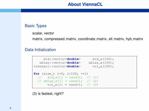
Basic Types
scalar, vector
matrix, compressed matrix, coordinate matrix, ell matrix, hyb matrix
Data Initialization
std::vector<double> std_x(100);ublas::vector<double> ublas_x(100);
viennacl::vector<double> vcl_x(100);
for (size_t i=0; i<100; ++i)// std_x[i] = rand(); // (1)// ublas_x[i] = rand(); // (2)
vcl_x[i] = rand(); // (3)
(3) is fastest, right?

9
About ViennaCLAbout ViennaCL
Basic Types
scalar, vector
matrix, compressed matrix, coordinate matrix, ell matrix, hyb matrix
Data Initialization
Using viennacl::copy()
std::vector<double> std_x(100);ublas::vector<double> ublas_x(100);
viennacl::vector<double> vcl_x(100);
/* setup of std_x and ublas_x omitted */
viennacl::copy(std_x.begin(), std_x.end(),vcl_x.begin()); //to GPU
viennacl::copy(vcl_x.begin(), vcl_x.end(),ublas_x.begin()); //to CPU
10
About ViennaCLAbout ViennaCL
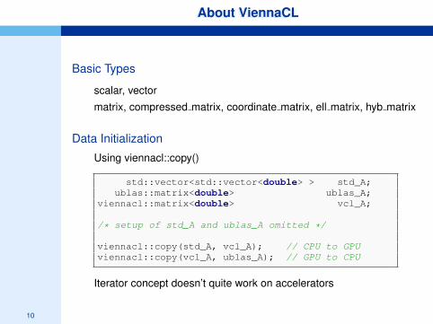
Basic Types
scalar, vector
matrix, compressed matrix, coordinate matrix, ell matrix, hyb matrix
Data Initialization
Using viennacl::copy()
std::vector<std::vector<double> > std_A;ublas::matrix<double> ublas_A;
viennacl::matrix<double> vcl_A;
/* setup of std_A and ublas_A omitted */
viennacl::copy(std_A, vcl_A); // CPU to GPUviennacl::copy(vcl_A, ublas_A); // GPU to CPU
Iterator concept doesn’t quite work on accelerators

11
InternalsInternals
Vector Addition
x = y + z;
Temporaries are costly (particularly on GPUs)
Expression Templates
Limited expansion
Map to a set of predefined kernels
vector_expression<vector<T>, op_plus, vector<T> >operator+(vector<T> & v, vector<T> & w) { ... }
vector::operator=(vector_expression<...> const & e) {viennacl::linalg::avbv(*this, 1,e.lhs(), 1,e.rhs());
}
12
BenchmarksBenchmarks
10-5
10-4
10-3
10-2
10-1
100
101
101
102
103
104
105
106
107
Execution T
ime (
sec)
Number of Unknowns
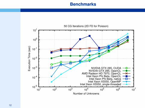
50 CG Iterations (2D FD for Poisson)
NVIDIA GTX 285, CUDANVIDIA GTX 285, OpenCL
AMD Radeon HD 7970, OpenCLIntel Xeon Phi Beta, OpenCL
Intel Xeon Phi Beta, nativeIntel Xeon X5550, OpenMP
Intel Xeon X5550, single-threaded

13
BenchmarksBenchmarks
Matrix-Matrix Multiplication
Autotuning environment
10
100
1000
10000
100 1000 10000
GF
LO
Ps
Matrix Rows/Columns
GFLOP Performance for GEMM (Higher is Better)
amdcl, out-of-the-boxViennaCL 1.4.0, out-of-the-box
ViennaCL, Work in Progress
(AMD Radeon HD 7970, single precision)

14
AcknowledgementsAcknowledgements
Contributors
Thomas Bertani
Evan Bollig
Philipp Grabenweger
Volodymyr Kysenko
Nikolay Lukash
Gunther Mader
Vittorio Patriarca
Florian Rudolf
Astrid Rupp
Philippe Tillet
Markus Wagner
Josef Weinbub
Michael Wild

15
SummarySummary
High-Level C++ Approach of ViennaCL
Convenience of single-threaded high-level libraries (Boost.uBLAS)
Header-only library for simple integration into existing code
MIT (X11) license
http://viennacl.sourceforge.net/
Selected Features
Backends: OpenMP, OpenCL, CUDA
Iterative Solvers: CG, BiCGStab, GMRES
Preconditioners: AMG, SPAI, ILU, Jacobi
BLAS: Levels 1-3

16
Part 2Part 2
PETSc
Portable Extensible Toolkit for Scientific Computing

17
PETScPETSc
Obtaining PETSc
Linux Package Managers
Web: http://mcs.anl.gov/petsc, download tarball
Git: https://bitbucket.org/petsc/petsc
Mercurial: https://bitbucket.org/petsc/petsc-hg
Installing PETSc
$> cd /path/to/petsc/workdir$> git clone \
https://bitbucket.org/petsc/petsc.git \--branch master --depth 1
$> cd petsc
$> export PETSC_DIR=$PWD PETSC_ARCH=mpich-gcc-dbg$> ./configure --with-cc=gcc --with-fc=gfortran
--download-f-blas-lapack--download-{mpich,ml,hypre}
18
PETScPETSc
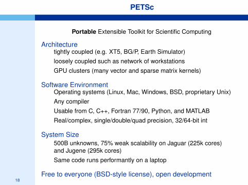
Portable Extensible Toolkit for Scientific Computing
Architecturetightly coupled (e.g. XT5, BG/P, Earth Simulator)
loosely coupled such as network of workstations
GPU clusters (many vector and sparse matrix kernels)
Software EnvironmentOperating systems (Linux, Mac, Windows, BSD, proprietary Unix)
Any compiler
Usable from C, C++, Fortran 77/90, Python, and MATLAB
Real/complex, single/double/quad precision, 32/64-bit int
System Size500B unknowns, 75% weak scalability on Jaguar (225k cores)and Jugene (295k cores)
Same code runs performantly on a laptop
Free to everyone (BSD-style license), open development

19
PETScPETSc
Portable Extensible Toolkit for Scientific Computing
Philosophy: Everything has a plugin architecture
Vectors, Matrices, Coloring/ordering/partitioning algorithms
Preconditioners, Krylov accelerators
Nonlinear solvers, Time integrators
Spatial discretizations/topology
Example
Vendor supplies matrix format and associated preconditioner,distributes compiled shared library.
Application user loads plugin at runtime, no source code in sight.

20
PETScPETSc
Portable Extensible Toolkit for Scientific Computing
Toolset
algorithms
(parallel) debugging aids
low-overhead profiling
Composability
try new algorithms by choosing from product space
composing existing algorithms (multilevel, domain decomposition,splitting)
Experimentation
Impossible to pick the solver a priori
PETSc’s response: expose an algebra of composition
keep solvers decoupled from physics and discretization

21
PETScPETSc
Portable Extensible Toolkit for Scientific ComputingComputational Scientists
PyLith (CIG), Underworld (Monash), Magma Dynamics (LDEO,Columbia), PFLOTRAN (DOE), SHARP/UNIC (DOE)
Algorithm Developers (iterative methods and preconditioning)
Package DevelopersSLEPc, TAO, Deal.II, Libmesh, FEniCS, PETSc-FEM, MagPar,OOFEM, FreeCFD, OpenFVM
FundingDepartment of Energy
SciDAC, ASCR ISICLES, MICS Program, INL Reactor ProgramNational Science Foundation
CIG, CISE, Multidisciplinary Challenge Program
Documentation and SupportHundreds of tutorial-style examples
Hyperlinked manual, examples, and manual pages for all routines
Support from [email protected]

22
Flow Control for a PETSc ApplicationFlow Control for a PETSc Application
Timestepping Solvers (TS)
Preconditioners (PC)
Nonlinear Solvers (SNES)
Linear Solvers (KSP)
Function
EvaluationPostprocessing
Jacobian
Evaluation
Application
Initialization
Main Routine
PETSc

23
PETSc PyramidPETSc Pyramid
PETSc Structure

24
Ghost ValuesGhost Values
To evaluate a local function f (x), each process requires
its local portion of the vector x
its ghost values, bordering portions of x owned by neighboringprocesses
Local Node
Ghost Node

25
DMDA Global NumberingsDMDA Global Numberings
Proc 2 Proc 325 26 27 28 2920 21 22 23 2415 16 17 18 1910 11 12 13 145 6 7 8 90 1 2 3 4
Proc 0 Proc 1Natural numbering
Proc 2 Proc 321 22 23 28 2918 19 20 26 2715 16 17 24 256 7 8 13 143 4 5 11 120 1 2 9 10
Proc 0 Proc 1PETSc numbering

26
DMDA Global vs. Local NumberingDMDA Global vs. Local Numbering
Global: Each vertex has a unique id, belongs on a unique processLocal: Numbering includes vertices from neighboring processes
These are called ghost vertices
Proc 2 Proc 3X X X X XX X X X X12 13 14 15 X8 9 10 11 X4 5 6 7 X0 1 2 3 X
Proc 0 Proc 1Local numbering
Proc 2 Proc 321 22 23 28 2918 19 20 26 2715 16 17 24 256 7 8 13 143 4 5 11 120 1 2 9 10
Proc 0 Proc 1Global numbering

27
Working with the Local FormWorking with the Local Form
Wouldn’t it be nice if we could just write our code for the naturalnumbering?
Proc 2 Proc 325 26 27 28 2920 21 22 23 2415 16 17 18 1910 11 12 13 145 6 7 8 90 1 2 3 4
Proc 0 Proc 1Natural numbering
Proc 2 Proc 321 22 23 28 2918 19 20 26 2715 16 17 24 256 7 8 13 143 4 5 11 120 1 2 9 10
Proc 0 Proc 1PETSc numbering

27
Working with the Local FormWorking with the Local Form
Wouldn’t it be nice if we could just write our code for the naturalnumbering?
Yes, that’s what DMDAVecGetArray() is for.
DMDA offers local callback functions
FormFunctionLocal(), set by DMDASetLocalFunction()
FormJacobianLocal(), set by DMDASetLocalJacobian()
Evaluating the nonlinear residual F(x)
Each process evaluates the local residualPETSc assembles the global residual automatically
Uses DMLocalToGlobal() method

28
The p-Bratu EquationThe p-Bratu Equation
p-Bratu Equation
2-dimensional model problem
−∇ ·(|∇u|p−2∇u
)− λeu − f = 0, 1 ≤ p ≤ ∞, λ < λcrit(p)
Singular or degenerate when ∇u = 0, turning point at λcrit.
Regularized Variant
Remove singularity of η using a parameter ε:
−∇ · (η∇u)− λeu − f = 0
η(γ) = (ε2 + γ)p−2
2 γ(u) =12|∇u|2
Physical interpretation: diffusivity tensor flattened in direction ∇u
29
ConclusionsConclusions
PETSc Can Help You
Solve algebraic and DAE problems in your application area
Rapidly develop efficient parallel code, can start from examples
Develop new solution methods and data structures
Debug and analyze performance
Advice on software design, solution algorithms, and performance
petsc-{users,dev,maint}@mcs.anl.gov
You Can Help PETSc
report bugs and inconsistencies, or if you think there is a better way
tell us if the documentation is inconsistent or unclear
consider developing new algebraic methods as plugins, contribute ifyour idea works
Top Related