


Languages
Pages
Legal

UvA-DARE is a service provided by the library of the University of Amsterdam (http://dare.uva.nl)
UvA-DARE (Digital Academic Repository)
Electrokinetics in porous media
Luong, D.T.
Link to publication
Citation for published version (APA):Luong, D. T. (2014). Electrokinetics in porous media.
General rightsIt is not permitted to download or to forward/distribute the text or part of it without the consent of the author(s) and/or copyright holder(s),other than for strictly personal, individual use, unless the work is under an open content license (like Creative Commons).
Disclaimer/Complaints regulationsIf you believe that digital publication of certain material infringes any of your rights or (privacy) interests, please let the Library know, statingyour reasons. In case of a legitimate complaint, the Library will make the material inaccessible and/or remove it from the website. Please Askthe Library: https://uba.uva.nl/en/contact, or a letter to: Library of the University of Amsterdam, Secretariat, Singel 425, 1012 WP Amsterdam,The Netherlands. You will be contacted as soon as possible.
Download date: 29 Aug 2019

Electrokinetics in porous media
ACADEMISCH PROEFSCHRIFT
ter verkrijging van de graad van doctor
aan de Universiteit van Amsterdam
op gezag van de Rector Magnificus
Prof. dr. D. C. van den Boom
ten overstaan van een door het college voor promoties
ingestelde commissie,
in het openbaar te verdedigen in de Agnietenkapel
op donderdag 09 Oktober 2014, te 12:00 uur.
door
Luong Duy Thanh
geboren te Thai Binh, Vietnam
i
Promotiecommissie:
Promotor: Prof. Dr. Daniel Bonn
Co-promotor: Dr. Rudolf Sprik
Overige leden:
Prof. Dr. Evert Slob
Prof. Dr. Holger Steeb
Prof. Dr. Sander Woutersen
Dr. Noushine Shahidzadeh
Faculteit der Natuurwetenschappen, Wiskunde en Informatica
Cover design by the author
@coppyright 2014 by Luong Duy Thanh. All rights reserved.
The author can be reached at:
The research reported in this thesis was carried out at the Van der Waals-Zeeman
Institute/Institute of Physics, University of Amsterdam. The work was financially
supported by Ministry of Education and Training (MOET) of Vietnam and partly
funded by Shell Oil Company and the Foundation for Fundamental Research on
Matter (FOM) in The Netherlands in the program for ’Innovative physics for oil
and gas’.

To my grandparents, my parents, my wife, my sons, my brothers, my nephews, my
nieces and my whole family.
Amsterdam, 15/08/2014
Luong Duy Thanh

Contents
Contents iii
Symbols vi
1 Introduction 11.1 Geophysical exploration . . . . . . . . . . . . . . . . . . . . . . . . 11.2 Physical chemistry of the electric double layer . . . . . . . . . . . . 31.3 Electrokinetics . . . . . . . . . . . . . . . . . . . . . . . . . . . . . . 6
1.3.1 Streaming potential (SP) . . . . . . . . . . . . . . . . . . . . 71.3.2 Electroosmosis (EO) . . . . . . . . . . . . . . . . . . . . . . 8
1.4 Microstructure parameters of porous media . . . . . . . . . . . . . . 101.5 Future works . . . . . . . . . . . . . . . . . . . . . . . . . . . . . . 121.6 The goal of this thesis . . . . . . . . . . . . . . . . . . . . . . . . . 14
2 Streaming potential and electroosmosis measurements to charac-terize porous materials 172.1 Introduction . . . . . . . . . . . . . . . . . . . . . . . . . . . . . . . 172.2 Experiment . . . . . . . . . . . . . . . . . . . . . . . . . . . . . . . 18
2.2.1 Porosity, permeability, formation factor measurements . . . . 192.2.2 Streaming potential measurement . . . . . . . . . . . . . . . 202.2.3 Electroosmosis measurement . . . . . . . . . . . . . . . . . . 20
2.3 Results and discussion . . . . . . . . . . . . . . . . . . . . . . . . . 212.3.1 Porosity, permeability, formation factor . . . . . . . . . . . . 212.3.2 Streaming Potential . . . . . . . . . . . . . . . . . . . . . . . 232.3.3 Electroosmosis . . . . . . . . . . . . . . . . . . . . . . . . . 24
2.4 Conclusions . . . . . . . . . . . . . . . . . . . . . . . . . . . . . . . 26
3 Permeability dependence of streaming potential coupling coeffi-cients 293.1 Introduction . . . . . . . . . . . . . . . . . . . . . . . . . . . . . . . 293.2 Experiment . . . . . . . . . . . . . . . . . . . . . . . . . . . . . . . 313.3 Results and discussion . . . . . . . . . . . . . . . . . . . . . . . . . 33
3.3.1 Porosity, solid density, permeability and formation factor . . 333.3.2 Streaming potential . . . . . . . . . . . . . . . . . . . . . . . 34
3.4 Conclusion . . . . . . . . . . . . . . . . . . . . . . . . . . . . . . . . 40
iii
Contents iv
4 Examination of a theoretical model of streaming potential cou-pling coefficient 434.1 Introduction . . . . . . . . . . . . . . . . . . . . . . . . . . . . . . . 434.2 Theoretical model of streaming potential . . . . . . . . . . . . . . . 454.3 Experiments . . . . . . . . . . . . . . . . . . . . . . . . . . . . . . . 474.4 Results and discussion . . . . . . . . . . . . . . . . . . . . . . . . . 50
4.4.1 Porosity, solid density, permeability and formation factor . . 504.4.2 Streaming potential as a function of electrolyte concentration 504.4.3 Streaming potential as a function of temperature . . . . . . 56
4.5 Conclusion . . . . . . . . . . . . . . . . . . . . . . . . . . . . . . . . 58
5 Zeta potential of porous rocks in contact with monovalent anddivalent electrolyte aqueous solutions 615.1 Introduction . . . . . . . . . . . . . . . . . . . . . . . . . . . . . . . 615.2 Theoretical background of the zeta potential . . . . . . . . . . . . . 63
5.2.1 For 1:1 electrolytes . . . . . . . . . . . . . . . . . . . . . . . 635.2.2 For 2:2 electrolytes . . . . . . . . . . . . . . . . . . . . . . . 645.2.3 For 1:2 or 2:1 electrolytes . . . . . . . . . . . . . . . . . . . 64
5.3 Experiments . . . . . . . . . . . . . . . . . . . . . . . . . . . . . . . 645.4 Results and discussion . . . . . . . . . . . . . . . . . . . . . . . . . 65
5.4.1 Streaming potential coupling coefficient versus electrolytetypes and and sample types . . . . . . . . . . . . . . . . . . 65
5.4.2 Zeta potential versus electrolyte types and sample types . . 655.5 Conclusion . . . . . . . . . . . . . . . . . . . . . . . . . . . . . . . . 72
6 Streaming potential measurements on the binary mixture Tri-ethylamine - water near the demixing phase transition 736.1 Introduction . . . . . . . . . . . . . . . . . . . . . . . . . . . . . . . 736.2 Experiments . . . . . . . . . . . . . . . . . . . . . . . . . . . . . . . 75
6.2.1 Setup . . . . . . . . . . . . . . . . . . . . . . . . . . . . . . 756.2.2 Materials . . . . . . . . . . . . . . . . . . . . . . . . . . . . 76
6.3 Results and discussion . . . . . . . . . . . . . . . . . . . . . . . . . 776.4 Conclusions . . . . . . . . . . . . . . . . . . . . . . . . . . . . . . . 82
A Parameters of porous samples 85A.1 Porosity . . . . . . . . . . . . . . . . . . . . . . . . . . . . . . . . . 85A.2 Solid density . . . . . . . . . . . . . . . . . . . . . . . . . . . . . . . 85A.3 Permeability . . . . . . . . . . . . . . . . . . . . . . . . . . . . . . . 86A.4 Tortuosity . . . . . . . . . . . . . . . . . . . . . . . . . . . . . . . . 87A.5 Frame and shear modulus . . . . . . . . . . . . . . . . . . . . . . . 87
B The equation to get the Stern potential for 2:2 electrolytes 93
Bibliography 97

Contents v
Summary 107
Samenvatting 111
Publications 114
Acknowledgements 115

Symbols
Symbol Description Units
T Temperature K
pH Fluid pH [-]
Cf Electrolyte concentration mol/L
CS Streaming potential coupling coefficient V/Pa
ζ Zeta potential V
η Dynamic viscosity of the fluid Pa.s
σeff Effective conductivity S/m
σf Fluid conductivity S/m
σS Conductivity of fluid saturated porous samples S/m
ρ∞i Ionic concentration of ions i in the solution C/m3
zi Valency of ions i [-]
χd Debye length m
a Average pore radius of porous samples m
ρf Fluid density kg/m3
g Acceleration due to gravity m/s2
ε0 Dielectric permittivity in vacuum F/m
εr Relative permittivity [-]
kb Boltzmann’s constant J/K
e Elementary charge C
N Avogadro’s number /mol
βNa+ Ionic mobility of Na+ in solution m2/s/V
βH+ Ionic mobility of H+ in solution m2/s/V
βCl− Ionic mobility of Cl− in solution m2/s/V
βOH− Ionic mobility of OH− in solution m2/s/V
Kw Disassociation constant of water [-]
Γs Surface site density sites/m2
KM Binding constant for Na+ adsorption [-]
vi

Symbols vii
K(−) Disassociation constant for dehydrogenization of surface sites [-]
cProt Proton surface conductance Sm2/site
βs Ionic Stern-plane mobility m2/s/V
φ Porosity of porous samples [-]
ko Permeability of porous samples m2
ρs Solid density of porous samples kg/m3
α∞ Tortuosity of porous samples [-]
F Formation factor of porous samples [-]
Σs Surface conductance of porous samples S
χζ Shear plane distance m
ϕd Stern potential V
ζo Zeta potential offset V
Qf Fluid volume flow rate m3/s
vP Compressional wave speed m/s
vS Shear wave speed m/s
KP Bulk modulus of porous samples Pa
KP Shear modulus of porous samples Pa
γ Poisson’s ratio [-]
Chapter 1
Introduction
1.1 Geophysical exploration
Electrokinetic phenomena are induced by the relative motion between a fluid and
a solid surface and are directly related to the existence of an electric double layer
between the fluid and the solid grain surface (see section 1.2). Electrokinetic phe-
nomena consist of several different effects such as seismoelectric effect, streaming
potential, electroosmosis, electrophoresis etc. (see section 1.3 for more detail).
Streaming potential and seismoelectric effects that arise due to fluids moving
through porous media (see subsection 1.3.1 for more detail) play an important
role in geophysical applications. For example, the streaming potential is used
to map subsurface flow and detect subsurface flow patterns in oil reservoirs [1].
Streaming potential is also used to monitor subsurface flow in geothermal areas
and volcanoes [2–4]. Monitoring of streaming potential anomalies has been pro-
posed as a means of predicting earthquakes [5, 6] and in studying water leakage
in water reservoirs [7]. In the environmental and engineering fields, self-potential
surveys related to streaming potential anomalies are used for the detection of seep-
age through water retention structures such as dams, dikes, reservoir floors, and
canals. Measurement of streaming potential provides information on the location,
flow magnitude and the depths and geometries and the direction of subsurface
flow paths in the structures.
Seismoelectric effects can be used in order to investigate oil and gas reservoirs
[8], hydraulic reservoirs [9–11] and downhole seismoelectric imaging [12]. In seis-
moelectric effects, a seismic source produces a seismic compression wave, which
then propagates into the ground with a seismic wave velocity depending on the
1

Chapter 1. Introduction 2
Figure 1.1: Schematic illustration of the seismoelectric exploration method. A seismicwave propagates into the ground and stresses a fluid saturated rock, for example. Therock converts some of the seismic energy to the seismmoelectric response that is detected
by electric or magnetic receivers
Figure 1.2: Schematic of the porous medium with different length scales: samplescale, grain scale and pore scale.
type of rocks through which it passes. When the initial pressure pulse reaches, for
example, a fluid saturated rock, the electrical signal is generated and transmit-
ted back to the ground surface at approximately the speed of light in the solid.
As a result, the delay between the shot moment and reception of the electrical
response is primarily due to the time taken by the seismic wave to travel from
the shot point to the target where the electrical signal (seismoelectric response) is
generated (see Fig. 1.1). The product of this delay with the seismic wave velocity
gives the distance from the source point to the target and the data from different
shot points can be used to determine location of the target. In addition, based on
the relationships between the spreading seismic wave and seismoelectric response
received by electrode arrays at the ground surface, one can determine the physical
properties of the liquid or the properties of liquid-solid systems.
Electroosmosis that arises due to the motion of liquid induced by an applied volt-
age across a porous material (see subsection 1.3.2 for more detail) is one of the
promising technologies for cleaning up low permeable soil in environmental appli-
cations. In this process, the contaminants are separated by the application of an

Chapter 1. Introduction 3
Figure 1.3: Stern model [3, 19, 20] for the charge and electric potential distributionin the electric double layer at a solid-liquid interface. In this figure, the solid surfaceis negatively charged and the mobile counter-ions in the diffuse layer are positively
charged (in most rock-water systems) [21, 22].
electric field between two electrodes inserted in the contaminated mass. Therefore,
it has been used for the removal of organic contaminants, petroleum hydrocarbons,
heavy metals and polar organic contaminants in soils, sludge and sediments by the
Holland Environment Group [13], for example (for more detail, see e.g. [14, 15]).
1.2 Physical chemistry of the electric double layer
Electrokinetic phenomena are the result of a coupling between fluid flow and elec-
tric current flow in a porous medium which is formed by mineral solid grains such
as silicates, oxides, carbonates (see Fig. 1.2). They arise due to a charge dis-
tribution known as the electric double layer (EDL) that exists at the solid-liquid
interface [16–18]. Most substances acquire a surface electric charge when brought
into contact with aqueous systems [16]. Although the presence of surface charges
is normally accepted without careful consideration of their origin in most elec-
trokinetic studies, it is still important to recognize the origin of these charges.
Surfaces may become electrically charged by a variety of mechanisms. Some of
the main mechanisms responsible for surface charges are (1) surface disassociation,
(2) ion adsorption from solution and (3) crystal lattice defects (for more detail,
see [16–18]).
To understand the origin of surface charge better, we consider the physical chem-
istry at a silica surface in the presence of the aqueous fluids. The reason for
Chapter 1. Introduction 4
considering a silica interface is that the silica is one of the most abundant min-
erals on the Earth’s crust [23]. Therefore it is the main mineral component of
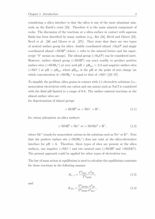
rocks. The discussion of the reactions at a silica surface in contact with aqueous
fluids has been described by many authors (e.g., Iler [24], Revil and Glover [25],
Revil et al. [26] and Glover et al. [27]). They state that there are two types
of neutral surface group for silica: doubly coordinated siloxal >Si2O0 and singly
coordinated silanol >SiOH0 (where > refer to the mineral lattice and the super-
script ”0” means no charge). The siloxal group (>Si2O0) can be considered inert.
However, surface silanol group (>SiOH0) can react readily to produce positive
surface sites (>SiOH2+) at very acid pH < pHpzc = 2-3 and negative surface sites
(>SiO−) at pH > pHpzc where pHpzc is the pH at the point of zero charge (at
which concentration of >SiOH2+ is equal to that of >SiO−)[25–27].
To simplify the problem, silica grains in contact with 1:1 electrolyte solutions (i.e.,
monovalent electrolytes with one cation and one anion) such as NaCl is considered
with the fluid pH limited to a range of 6-8. The surface mineral reactions at the
silanol surface sites are:
for deprotonation of silanol groups
> SiOH0 ⇔ > SiO− +H+, (1.1)
for cation adsorption on silica surfaces
> SiOH0 +Me+ ⇔ > SiOMe0 +H+, (1.2)
where Me+ stands for monovalent cations in the solutions such as Na+ or K+. Note
that the positive surface site (>SiOH2+) does not exist at the silica-electrolyte
interface for pH > 6. Therefore, three types of sites are present at the silica
surfaces, one negative (>SiO−) and two neutral ones (>SiOH0 and >SiOMe0).
The present approach could be applied for other types of electrolytes too.
The law of mass action at equilibrium is used to calculate the equilibrium constants
for those reactions in the following manner
K(−) =Γ0
SiO− .α0H+
Γ0SiOH
, (1.3)
and
KMe =Γ0
SiOMe.α0H+
Γ0SiOH.α0
Me+, (1.4)

Chapter 1. Introduction 5
where K(−) is the disassociation constant for deprotonation of silanol surface sites,
KMe is the binding constant for cation adsorption on the silica surfaces, Γ0i is the
surface site density of surface species i in sites/m2 and α0i is the activity of an
ionic species i at the closest approach of the mineral surface.
The total surface site density (Γ0s) is constant
Γ0s = Γ0
SiOH + Γ0SiO− + Γ0
SiOMe. (1.5)
Eq. (1.5) is a conservation equation for mineral surface groups. From Eq.(1.3)-
Eq.(1.5), the surface site density of sites Γ0SiO− and Γ0
SiOMe are obtained. The
mineral surface charge density Q0s in C/m2 can be found by summing the surface
densities of charged surface groups (only one charged surface group in this problem
- Γ0SiO−) as
Q0s = −e.Γ0
SiO− , (1.6)
where e is the elementary charge.
The mineral surface charge repels ions in the electrolyte whose charges have the
same sign as the surface charge (called the ”coions”) and attracts ions whose
charges have the opposite sign (called the ”counterions” and normally cations) in
the vicinity of the electrolyte-silica interface. This leads to the charge distribution
known as the electric double layer (EDL) (see Fig. 1.3). The EDL is made up
of the Stern layer, where cations are adsorbed on the surface and are immobile
due to the strong electrostatic attraction, and the diffuse layer, where the ions
are mobile. The distribution of ions and the electric potential within the diffuse
layer is governed by the Poisson-Boltzman (PB) equation which accounts for the
balance between electrostatic and thermal diffusional forces [16]. The solution to
the linear PB equation in one dimension perpendicular to a broad planar interface
is well-known and produces an electric potential profile that decays approximately
exponentially with distance as shown in Fig. 1.3. In the bulk liquid, the number
of cations and anions is equal so that it is electrically neutral. The closest plane
to the solid surface in the diffuse layer at which flow occurs is termed the shear
plane or the slipping plane, and the electrical potential at this plane is called the
zeta potential (ζ). As shown below, the zeta potential plays an important role in
determining magnitude of electrokinetic phenomena. Most reservoir rocks have a
negative surface charge and a negative zeta potential when in contact with ground
water [21, 22]. The characteristic length over which the EDL exponentially decays
is known as the Debye length (for more detail, see [12, 28]). It should be noted
that the Debye length depends solely on the properties of the liquid and not on

Chapter 1. Introduction 6
Figure 1.4: Development of streaming potential when an electrolyte is pumpedthrough a capillary (a porous medium is made of an array of parallel capillaries).
the properties of the surface such as its charge or potential and it is given by [29]
χd =
√ε0εrkbT∑ρ∞ie2z2i
, (1.7)
where kb is the Boltzmann’s constant, T is temperature (in K), ε0 is the dielectric
permittivity in vacuum, εr is the relative permittivity of fluids, ρ∞i is the ionic
concentration of ions i in the solution, e is the elementary charge and zi is the
valency of ions i.
For monovalent electrolytes (e.g., NaCl or KCl ) with concentrations in the range
of 1 mM to 0.1 M (typical concentrations for aqueous solutions saturating rocks
or soils), the Debye length varies between 10 nm and 1 nm at 25◦C [29]. The
Debye length is typically much smaller than pore sizes of a majority of rocks and
soils. Therefore, the solid-liquid interface in the pores can be considered planar
and semi-infinite space.
1.3 Electrokinetics
Electrokinetic phenomena are a family of several different effects (e.g., streaming
potential, electroosmosis, electrophoresis and etc.) that occur in fluids containing
particles, or in porous media filled with fluid, or in a fast flow over a flat surface
(for more details, see [18]). Electrokinetic phenomena are induced by the relative
motion between the fluid and a charged surface under application of an external
force, and they are directly related to the existence of an electric double layer be-
tween the fluid and the solid surface (see section 1.2 for more detail). This external
force might be electric, pressure gradient, concentration gradient, or gravity. In
the scope of this thesis, we just focus on streaming potential and electroosmosis
effects happening in the porous media saturated by electrolytic fluids.
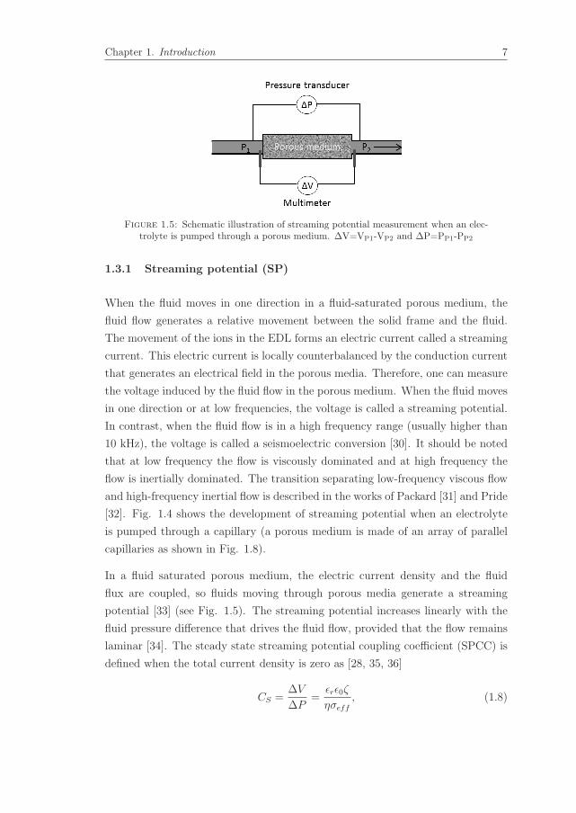
Chapter 1. Introduction 7
Figure 1.5: Schematic illustration of streaming potential measurement when an elec-trolyte is pumped through a porous medium. ΔV=VP1-VP2 and ΔP=PP1-PP2
1.3.1 Streaming potential (SP)
When the fluid moves in one direction in a fluid-saturated porous medium, the
fluid flow generates a relative movement between the solid frame and the fluid.
The movement of the ions in the EDL forms an electric current called a streaming
current. This electric current is locally counterbalanced by the conduction current
that generates an electrical field in the porous media. Therefore, one can measure
the voltage induced by the fluid flow in the porous medium. When the fluid moves
in one direction or at low frequencies, the voltage is called a streaming potential.
In contrast, when the fluid flow is in a high frequency range (usually higher than
10 kHz), the voltage is called a seismoelectric conversion [30]. It should be noted
that at low frequency the flow is viscously dominated and at high frequency the
flow is inertially dominated. The transition separating low-frequency viscous flow
and high-frequency inertial flow is described in the works of Packard [31] and Pride
[32]. Fig. 1.4 shows the development of streaming potential when an electrolyte
is pumped through a capillary (a porous medium is made of an array of parallel
capillaries as shown in Fig. 1.8).
In a fluid saturated porous medium, the electric current density and the fluid
flux are coupled, so fluids moving through porous media generate a streaming
potential [33] (see Fig. 1.5). The streaming potential increases linearly with the
fluid pressure difference that drives the fluid flow, provided that the flow remains
laminar [34]. The steady state streaming potential coupling coefficient (SPCC) is
defined when the total current density is zero as [28, 35, 36]
CS =ΔV
ΔP=
εrε0ζ
ησeff
, (1.8)
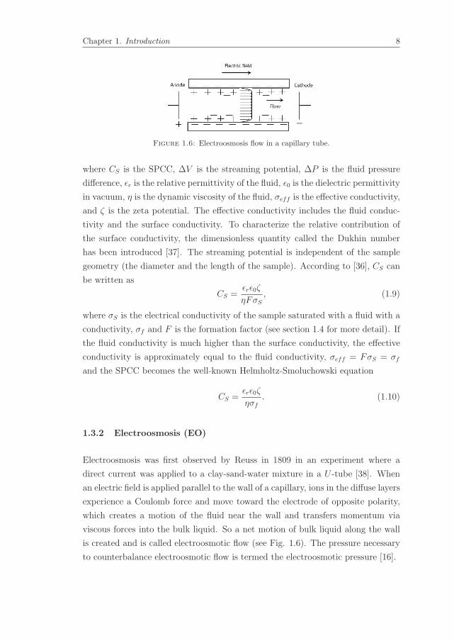
Chapter 1. Introduction 8
Figure 1.6: Electroosmosis flow in a capillary tube.
where CS is the SPCC, ΔV is the streaming potential, ΔP is the fluid pressure
difference, εr is the relative permittivity of the fluid, ε0 is the dielectric permittivity
in vacuum, η is the dynamic viscosity of the fluid, σeff is the effective conductivity,
and ζ is the zeta potential. The effective conductivity includes the fluid conduc-
tivity and the surface conductivity. To characterize the relative contribution of
the surface conductivity, the dimensionless quantity called the Dukhin number
has been introduced [37]. The streaming potential is independent of the sample
geometry (the diameter and the length of the sample). According to [36], CS can
be written as
CS =εrε0ζ
ηFσS
, (1.9)
where σS is the electrical conductivity of the sample saturated with a fluid with a
conductivity, σf and F is the formation factor (see section 1.4 for more detail). If
the fluid conductivity is much higher than the surface conductivity, the effective
conductivity is approximately equal to the fluid conductivity, σeff = FσS = σf
and the SPCC becomes the well-known Helmholtz-Smoluchowski equation
CS =εrε0ζ
ησf
. (1.10)
1.3.2 Electroosmosis (EO)
Electroosmosis was first observed by Reuss in 1809 in an experiment where a
direct current was applied to a clay-sand-water mixture in a U -tube [38]. When
an electric field is applied parallel to the wall of a capillary, ions in the diffuse layers
experience a Coulomb force and move toward the electrode of opposite polarity,
which creates a motion of the fluid near the wall and transfers momentum via
viscous forces into the bulk liquid. So a net motion of bulk liquid along the wall
is created and is called electroosmotic flow (see Fig. 1.6). The pressure necessary
to counterbalance electroosmotic flow is termed the electroosmotic pressure [16].

Chapter 1. Introduction 9
Figure 1.7: Schematic of experimental setup for electroosmosis measurements inwhich Δh and R are height difference of liquid, the radius of the tubes in both sides,
respectively.
A complex porous sample with the physical length L and cross sectional area A
can be approximated as an array of N parallel capillaries with inner radius equal
to the average pore radius a of the medium and an equal value of zeta potential
ζ. For each of these idealized capillaries, the solution for electroosmotic flow in a
single tube can be analyzed to estimate the behavior of the total flow in a porous
medium by integrating over all pores [39].
In a U -tube experiment, when an electric potential difference is applied across the
fluid saturated porous medium, the liquid rises on one side (the cathode compart-
ment for our experiment) and lowers on the other side (the anode compartment).
This height difference increases with the time and this process stops when the hy-
draulic pressure caused by the height difference equals the electroosmosis pressure
(see Fig. 1.7). At that time the height difference is maximum.
The expression for the height difference Δh as a function of time is given by [14]
Δh =ΔPeq
ρfg
[1− exp(−Nρfga
4
4ηR2Lt)
]=
ΔPeq
ρfg
[1− exp(− t
τ)
], (1.11)
with
ΔPeq =8εrε0|ζ|V
a2
[1− 2χdI1(a/χd)
aI0(a/χd)
], (1.12)
and
τ =4ηR2L
Nρfga4, (1.13)

Chapter 1. Introduction 10
where τ is response time, ΔPeq is the pressure difference caused by the electroos-
mosis flow at equilibrium which corresponds to maximum height difference, V is
the applied voltage across the porous medium, ρf is the fluid density, g is the
acceleration due to gravity, χd is the Debye length, R is the radius of the tubes in
both sides, I0 and I1 are the zero-order and the first-order modified Bessel function
of the first kind, respectively.
For a conductive liquid, the Debye length χd is about 1 nm as mentioned in Section
1.2 and a typical pore radius of the samples a is in the order of μm. In this case
the ratio I1(a/χd)/I0(a/χd) can be neglected [40]. Under these conditions, Eq.
(1.12) may be simplified to
ΔPeq =8εrε0|ζ|V
a2, (1.14)
and Eq. (1.11) can be rewritten as follows
Δh =8εrε0|ζ|Vρfga2
[1− exp(− t
τ)
]= Δhmax
[1− exp(− t
τ)
], (1.15)
with
Δhmax =8εrε0|ζ|Vρfga2
. (1.16)
1.4 Microstructure parameters of porous media
In this section, we present definitions of microstructure parameters to describe
porous media such as the porosity, permeability, tortuosity, formation factor and
solid density. Those parameters will be mentioned throughout this thesis.
Porosity
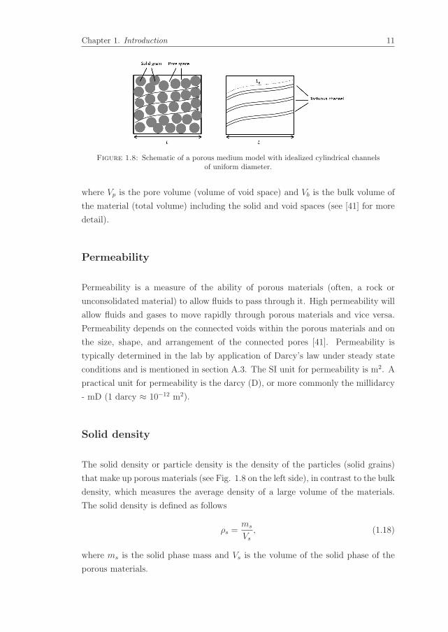
Porosity is a measure of the void spaces in a porous material, and is a fraction of
the volume of voids over the total volume, between 0 and 1, or as a percentage
between 0 and 100 % (see Fig. 1.8 on the left side). It is given by
φ =Vp
Vb
, (1.17)
Chapter 1. Introduction 11
Figure 1.8: Schematic of a porous medium model with idealized cylindrical channelsof uniform diameter.
where Vp is the pore volume (volume of void space) and Vb is the bulk volume of
the material (total volume) including the solid and void spaces (see [41] for more
detail).
Permeability
Permeability is a measure of the ability of porous materials (often, a rock or
unconsolidated material) to allow fluids to pass through it. High permeability will
allow fluids and gases to move rapidly through porous materials and vice versa.
Permeability depends on the connected voids within the porous materials and on
the size, shape, and arrangement of the connected pores [41]. Permeability is
typically determined in the lab by application of Darcy’s law under steady state
conditions and is mentioned in section A.3. The SI unit for permeability is m2. A
practical unit for permeability is the darcy (D), or more commonly the millidarcy
- mD (1 darcy ≈ 10−12 m2).
Solid density
The solid density or particle density is the density of the particles (solid grains)
that make up porous materials (see Fig. 1.8 on the left side), in contrast to the bulk
density, which measures the average density of a large volume of the materials.
The solid density is defined as follows
ρs =ms
Vs
, (1.18)
where ms is the solid phase mass and Vs is the volume of the solid phase of the
porous materials.
Chapter 1. Introduction 12
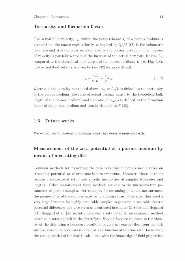
Tortuosity and formation factor
The actual fluid velocity, va, within the pores (channels) of a porous medium is
greater than the macroscopic velocity, v, implied by Qf/A (Qf is the volumetric
flow rate and A is the cross sectional area of the porous medium). The increase
of velocity is partially a result of the increase of the actual flow path length, Le,
compared to the theoretical bulk length of the porous medium, L (see Fig. 1.8).
The actual fluid velocity is given by (see [42] for more detail)
va =v
φ
Le
L=
v
φα∞, (1.19)
where φ is the porosity mentioned above, α∞ = Le/L is defined as the tortuosity
of the porous medium (the ratio of actual passage length to the theoretical bulk
length of the porous medium) and the ratio of α∞/φ is defined as the formation
factor of the porous medium and usually denoted as F [43].
1.5 Future works
We would like to present interesting ideas that deserve more research.
Measurement of the zeta potential of a porous medium by
means of a rotating disk
Common methods for measuring the zeta potential of porous media relies on
streaming potential or electroosmosis measurements. However, those methods
require a complicated setup and specific geometries of samples (diameter and
length). Other limitations of those methods are due to the microstructure pa-
rameters of porous samples. For example, for streaming potential measurement
the permeability of the samples must be in a given range. Otherwise, they need a
very large flow rate for highly permeable samples to generate measurable electric
potential differences and vice versa as mentioned in chapter 3. Sides and Hoggard
[44], Hoggard et al. [45] recently described a zeta potential measurement method
based on a rotating disk in the electrolyte. Solving Laplace equation in the vicin-
ity of the disk using a boundary condition of zero net current flow from the disk
surface, streaming potential is obtained as a function of rotation rate. From that,
the zeta potential of the disk is calculated with the knowledge of fluid properties.
Chapter 1. Introduction 13
Based on the same ideas of [44, 45], we are developing a new setup with an array
of 64 electrodes in stead of 2 electrodes as used in [44, 45]. With that setup, an
electric potential distribution beneath a rotating disk will be drawn and compared
to the theoretical predictions. From the electric potential distribution, the zeta
potential can be calculated.
The streaming potential of liquid carbon dioxide in porous
media
In response to global climate change caused by the buildup of greenhouse gasses
such as carbon dioxide (CO2), Carbon dioxide capture and storage technology
(CCS) has been used to mitigate CO2 emissions from the atmosphere. CCS is the
process of capturing waste CO2 from large point sources, such as fossil fuel power
plants, transporting it to a storage site, and depositing it where it will not enter
the atmosphere, normally an underground geological formation. For reasons such
as leakage of CO2 to the groundwater or to the atmosphere, monitoring subsurface
storage of CO2 to know migration paths of CO2 and CO2 leakages at the surface
is very important. Streaming potential is proposed as one of the methods for
identifying flow paths of CO2 through the rock matrix and measuring the change
in electrokinetic parameters due to CO2 migration [46].
During CO2 infiltration through porous rocks weak carbonic acid is formed, this
results in the change of the pH and the electrical resistivity of the pore water.
In addition, carbonic acid may dissolve some minerals that are present in rocks
and this leads to change of pore frame and therefore the change of permeability
and porosity of rocks. All parameters affect the SPCC and the zeta potential.
Therefore, we also want to use knowledge in this thesis to fully understand how
the the SPCC and the zeta potential behave in porous media during liquid CO2
injection.
Moore et al. [46] stated that even all mobile water is drained, ”trapped water”
still remains in the pores for Berea sandstone. Therefore, we would like to know if
there is a coupling between the fluid flow and electric current when nonconductive
liquid CO2 occupies and displaces all mobile pore water in porous samples. If yes,
we want to understand which parameters the SPCC depends on in this case.

Chapter 1. Introduction 14
1.6 The goal of this thesis
The streaming potential is a special case of the seismoelectric conversion at con-
stant flow rate or at low frequency. If the streaming potential in porous media
is understood, seismoelectric conversion could be effectively applied in order to
investigate oil, gas and hydraulic reservoirs, for example. Therefore, in this thesis
we mainly focus on characterizing porous media based on the streaming potential
and electroosmotic measurements and we specifically study the dependence of the
streaming potential on the permeability of rocks, the electrolyte concentration,
temperature, types of electrolyte and types of rocks. Streaming potential mea-
surements on the binary mixture triethylamine - water near the demixing phase
transition is also studied. This thesis is organized as follows:
The coupling coefficients of conversion between seismic wave and electromagnetic
wave depend strongly on microstructure parameters of porous media. Therefore,
in chapter 2 we use dc measurements of streaming potential and electroosmosis in
porous samples to characterize porous media. We can determine the parameters
such as the zeta potential, pore size, the number of pores per cross sectional
area of porous samples, porosity and permeability that are very important for the
experimental study of the seismoelectric effect.
In chapter 3, we study the permeability dependence of the streaming potential
coupling coefficient (SPCC) including the effects of the difference in the zeta po-
tential between samples and the change of surface conductance against electrolyte
concentration. To do so, the ratio of the SPCC and zeta potential is used rather
than the SPCC only. The results have shown that the SPCC strongly depends on
permeability of the samples for low fluid electrical conductivity. However, when
the fluid conductivity is larger than a certain value, the SPCC is completely inde-
pendent of permeability. The results are explained by the surface conductivity of
the rocks.
A comparison of existing theoretical models to experimental data sets from pub-
lished data for streaming potentials is also performed. However, the existing ex-
perimental data sets are based on samples with dissimilar fluid conductivity, pH
of pore fluid, temperature, and sample compositions. Those dissimilarities may
cause the observed deviations between theory and experiment. In chapter 4, we
critically assess the models by carrying out streaming potential measurement as a
function of electrolyte concentration and temperature for a set of well-defined con-
solidated samples and compare the results in a consistent manner with the models.

Chapter 1. Introduction 15
The results show that the existing theoretical models are not in good agreement
with the experimental observations when varying the electrolyte concentration,
especially at low electrolyte concentration. However, if we use a modified model
in which the zeta potential is assumed constant over the electrolyte concentration,
the model fits the experimental data well over a large range of concentrations.
The observed temperature dependence shows that the theoretical models are not
fully adequate to describe the experimental data but does describe correctly the
increasing trend of the SPCC as function of temperature.
In chapter 5, the dependence of zeta potential of porous rocks on types of elec-
trolytes (monovalent and divalent electrolyte aqueous solutions) are experimentally
and theoretically studied. The results show that the SPCC and the zeta potential
strongly depend on the mineral composition and types of electrolyte. The zeta
potential for monovalent electrolytes is higher than that for divalent electrolytes
for a given rock.
For critical binary mixtures with phase transition, the large density fluctuations
that develope near the demixing phase transition affect many physical parameters
directly related to the SPCC such as viscosity, electrical conductivity and dielectric
constant. Beside the change of the physical parameters, the properties of the
electric double layer and the debye length are expected to behave differently near
the demixing phase transition. In chapter 6, streaming potential measurements
are performed with a binary mixture through a porous material. Measurements on
such systems are unique and the behavior is not available in the existing literature
at all. The binary mixture triethylamine-water (TEA-W) with three different mass
fractions of TEA are used. This mixture is known to be a typical partially miscible
system that has a lower critical solution temperature that splits into two phases
with a temperature increase. The results show that the zeta potential changes
with composition of TEA and temperature. Interestingly, an anomaly of the zeta
potential near the critical point is observed for the critical composition. Therefore,
there may be an anomalous change of the electric double layer near the critical
point.
In Appendix A, we present the methods and the experimental setups to measure
the porosity φ, density of grains ρs, tortuosity α∞, formation factor F and steady-
state permeability ko of porous samples including unconsolidated samples and
consolidated samples. In addition, we also show laboratory measurement of the
frame and shear modulus of the consolidated samples (KP and GS).

Chapter 1. Introduction 16
In Appendix B, we derive an expression to calculate the zeta potential for diva-
lent electrolytes that has been used in chapter 5 based on the same procedures
mentioned in [25–27] for monovalent electrolytes.
Chapter 2
Streaming potential and
electroosmosis measurements to
characterize porous materials
2.1 Introduction
The coupling coefficient of conversion between seismic wave and electromagnetic
wave depends strongly on the fluid conductivity, porosity, permeability, forma-
tion factor, pore size, zeta potential of porous media and other properties of the
rock formation [32]. Therefore, determining these parameters is very important in
studying electrokinetics in general and to model seismoelectric and electroseismic
conversions. Li et al. [47] used ac measurements of streaming potential and elec-
troosmosis to determine the effective pore size and permeability of porous media.
Paillat et al. [14] used image analysis to determine the number of pores per cross
sectional area of porous samples (pore density). The pore density is especially im-
portant in processes of contaminant removal from low permeability porous media
under a dc electric field [14] and in building electroosmosis micropumps [48].
However, the method used in [14] did not work for porous media with very small
pores such as Bentonite clay soils or tight-gas sandstones (the pore radius is smaller
than 1 μm) that are relevant for application in the oil and gas industry [49]. In
oil exploration and production, the typical pore sizes in rocks is the necessary
information for considering the location of oil and fluid flow through the rocks.
The characteristics of porous media also determine differential gas pressures needed
to overcome capillary resistance of tight-gas sandstones in gas production.
17
Chapter 2. Streaming potential and electroosmosis measurements to characterizeporous materials 18
Alternative methods such as nuclear magnetic resonance (NMR) or magnetic res-
onance imaging (IRM) can also be used to determine characteristics of porous
media such as the porosity and pore size distribution, the permeability and the
water saturation [50]. But this technique is quite expensive and is not able to
determine the zeta potential - one of the most important parameters in electroki-
netic phenomena. In this chapter, we use dc measurements of streaming potential
and electroosmosis in porous samples and other simple measurements to fully
characterize porous media and determine parameters needed for the study of seis-
moelectric and electroseismic conversions. The approach works in particular well
for very small pore samples.
This chapter has three sections. Section 2.2 presents the investigated samples
and the experimental methods. Section 2.3 contains the experimental results and
discussion. Conclusions are provided in Section 2.4.
2.2 Experiment
To demonstrate that characterization of porous media can be done by obtaining
parameters such as porosity, permeability, formation factor, pore size, the number
of pores and zeta potential of porous media through electrokinetics, streaming
potential and electroosmosis measurements have been performed on 7 unconsol-
idated samples. Six are packs of spherical monodisperse particle with different
diameters of the particles (10 μm, 20 μm, 40 μm, 140 μm, 250 μm and 500 μm).
The monodisperse particles are obtained from Microbeads AS company, and are
composed of polystyrene polymers. Those samples are designated as TS10, TS20,
TS40, TS140, TS250 and TS500, respectively. It should be noted that the sample
designated TS10 corresponds to the one with 10 μm particles and the similar for
other samples. Beside monodisperse particle samples, we also use an unconsoli-
dated sample made up of blasting sand particles obtained from Unicorn ICS BV
company with diameter in the range of 200-300 μm (designated as Ssand).
Samples are constructed by filling polycarbonate plastic tubes (1 cm in inner
diameter and 7.5 cm in length) successively with 2 cm thick layers of particles
that are gently tamped down and shake by a shaker (TIRA-TV52110). Filter
paper is used in both ends of the tube to retain the particles and is permeable
enough to let the fluid pass through. The samples are then flushed with deionized
water to remove any powder or dust.

Chapter 2. Streaming potential and electroosmosis measurements to characterizeporous materials 19
Figure 2.1: Set up for measuring the electrical conductivity of a porous mediumsaturated with an electrolyte on the right. On the left hand side is the identical setup
without the porous medium for measuring the fluid conductivity.
We use a 10−3M NaCl solution of low enough conductivity of 10 × 10−3 S/m
measured by the conductivity meter (Consort C861) for the measurements. All
measurements are carried out at room temperature (22 ± 1◦C). When using low
electrical conductivity solutions such as deionized water, the magnitude of the
streaming potential coupling coefficient (SPCC) is large. However, the electri-
cal conductivity of the saturated samples slowly stabilizes in about 24h for our
samples. Perhaps due to CO2 uptake from the air, that changes the conductivity.
2.2.1 Porosity, permeability, formation factor measurements
The way to measure the porosity, permeability of porous samples are the same
as described in Appendix A for consolidated samples. Method of determining the
tortuosity was proposed by Brown [51]. The formation factor F is defined as:
F =α∞φ
=σf
σS
, (2.1)
where α∞ is the tortuosity, φ is the porosity of the sample, σf is the fluid con-
ductivity and σS is the electrical conductivity of the fluid saturated sample. It
should be noted that Eq. 2.1 is valid when surface conductivity effects become
negligible (at high fluid conductivities, σf ). For unconsolidated samples, we use
the experimental setup similar to the one described in [52] and is shown in Fig.
2.1. The electrodes, Ag/AgCl mesh disks, are placed on both sides against the
porous sample that is saturated successively with a set of aqueous NaCl solutions
with different conductivities (0.13, 0.47, 0.81, 1.23, 1.51 and 1.98 S/m). The con-
ductivities of those solutions are much higher than surface conductivity of the
material, so the surface conductivity is negligible (for more detail, see [53]). The
electrical conductivity is deduced form the resistance measurement using a Hioki
IM3570 impedance analyzer at different frequencies (varying from 100Hz to 100
kHz).
Chapter 2. Streaming potential and electroosmosis measurements to characterizeporous materials 20
Figure 2.2: Experimental setup for streaming potential measurements
2.2.2 Streaming potential measurement
The experimental setup for the measurement of the streaming potential is shown
in Fig. 2.2. The pressure differences across the sample are created by a high pres-
sure pump (LabHut, Series III- Pump) and measured by a pressure transducer
(Endress and Hauser Deltabar S PMD75). The electrical potential is measured by
two Ag/AgCl wire electrodes (A-M systems). The electrodes are put in the vicin-
ity of the end faces of the sample but not within the liquid circulation to avoid the
electrical noise from liquid movement around the electrodes [36]. The electrolyte
from the outlet tube is not in contact with electrolyte used to pump liquid through
the samples, preventing an electric current leakage through the liquid in the tube.
The solution is circulated through the samples until the electrical conductivity
and pH of the solution reache a stable value. Electrical potentials across the sam-
ples are then measured by a high input impedance multimeter (Agilent 34401A)
connected to a computer and controlled by a Labview program (National Instru-
ments). The electrical potentials at a given pressure difference fluctuate around
a specific value as shown in Fig. 2.5. The Labview program averages the value
of electrical potentials. The pH of equilibrium solutions, measured with the pH
meter (Consort C861), are in the range of 7.1 to 7.6 and the solutions are also
used for electroosmosis measurements.
2.2.3 Electroosmosis measurement
The experimental setup for the electroosmosis measurement is shown in Fig. 1.7.
The same solution which was used in the streaming potential measurement is also
used for this measurement. The zeta potential is consequently the same for both

Chapter 2. Streaming potential and electroosmosis measurements to characterizeporous materials 21
Figure 2.3: The flow rate against pressure difference. Two runs are shown for sampleTS10.
kinds of measurements. The electrodes used to apply a dc voltage across the
samples are perforated Ag/AgCl electrodes (MedCaT). To measure the maximum
height difference, Δhmax , and the height difference as a function of time at a
given voltage, cameras (Philips SPC 900NC PC) with the assistance of HandiAVI
software are used to take pictures of the heights of the liquid columns over time.
For each new measurement (new applied voltage, new sample) the samples are
dried, mounted in the setup, evacuated by a vacuum pump and fully saturated by
the same solutions.
It should be noted that when an applied voltage exceeds a critical value (1.48V
for water [54]), there will be electrolysis at the anode and the cathode. These
electrode reactions produce ions and gas in both electrodes. If these ions are not
removed, these reactions induce a low in pH at the anode and a high pH at the
cathode and a change in electrical conductivity. The rate of electrolysis reaction
is largely determined by the current. If the current density is smaller than < 35
μA per cm2 cross sectional area, the effects due to the electrolysis can be ignored
[55]. The resistances of the fully saturated samples that we use in this chapter
are about 400 kΩ, so applied voltages are limited below 10V to avoid unwanted
electrolysis effects.
2.3 Results and discussion
2.3.1 Porosity, permeability, formation factor
The measured porosity of the packs is 0.39 independently of the size of the particles
with an error of 5%. Fig. 2.3 shows the typical graph of flow rate as a function of
applied pressure difference for sample TS10.

Chapter 2. Streaming potential and electroosmosis measurements to characterizeporous materials 22
Table 2.1: Measured properties of the samples. In which d, ko, F and σS are diameter,permeability, formation factor and electrical conductivity of the saturated samples at
equilibrium for all samples, respectively.
Sample d (in μm) ko (in m2 ) F σS (in S/m)
TS10 10 0.15 ×10⁻¹² 4.0 4.1 ×10⁻³
TS20 20 0.30 ×10⁻¹² 4.2 3.6 ×10⁻³
TS40 40 0.85 ×10⁻¹² 4.2 3.0 ×10⁻³
TS140 140 1.36 ×10⁻¹² 4.3 3.1 ×10⁻³
TS250 250 1.71 ×10⁻¹² 4.0 3.5 ×10⁻³
TS500 500 2.36 ×10⁻¹² 4.3 2.9 ×10⁻³
Ssand 200-300 1.22 ×10⁻¹² 4.0 3.0 ×10⁻³
Figure 2.4: Saturated sample conductivity versus electrolyte conductivity for 2 sam-ples (red dots for TS10 and blue cross symbols for TS500). The slopes of the straight
lines yield the formation factors
The graph shows that there is a linear relationship between flow rate and pressure
difference and Darcy’s law is obeyed. So the flow is laminar and Eq. (1.8) and Eq.
(1.9) are valid. This behavior is identical for all samples. Two measurements are
performed for all samples to find the graphs of flow rate versus pressure difference.
From the slope of the graph and Darcy’s law (the viscosity of the fluid is taken as
10−3 Pa.s), the permeability of the sample is calculated. We obtain permeabilities
of all samples (see Table 2.1) with an uncertainty of 15% of the reported values.
An example of the electrical conductivity of the saturated samples versus the
electrical conductivity of the electrolyte is shown in Fig. 2.4 for the 2 samples
with the largest differences in the formation factors. We calculate the formation
factor F as the reciprocal of the slope of a linear regression through the data
points. Values of the formation factors for all samples are also reported in Table
2.1 with an error of 5%.
The measured formation factor of the samples is the range of 4.0 to 4.3 (see Table
Chapter 2. Streaming potential and electroosmosis measurements to characterizeporous materials 23
Figure 2.5: The electrical potential (V) fluctuating with time (s) at a given pressuredifference for sample TS10 is taken by Labview.
2.1). According to Archie’s law [56], F = φ−m (F is the formation factor, φ is
the porosity of the sample and m is the so-called cementation exponent), m is
found to be in the range 1.47-1.55. For unconsolidated samples made of perfect
spheres, the exponent m should be 1.5 [57]. So the measured formation factors of
the samples are in good agreement with Archie’s law. The electrical conductivities
of the samples saturated by the solutions are also shown in Table 2.1.
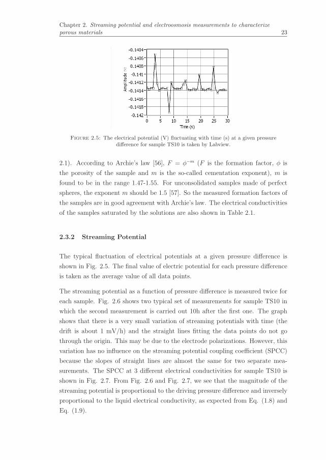
2.3.2 Streaming Potential
The typical fluctuation of electrical potentials at a given pressure difference is
shown in Fig. 2.5. The final value of electric potential for each pressure difference
is taken as the average value of all data points.
The streaming potential as a function of pressure difference is measured twice for
each sample. Fig. 2.6 shows two typical set of measurements for sample TS10 in
which the second measurement is carried out 10h after the first one. The graph
shows that there is a very small variation of streaming potentials with time (the
drift is about 1 mV/h) and the straight lines fitting the data points do not go
through the origin. This may be due to the electrode polarizations. However, this
variation has no influence on the streaming potential coupling coefficient (SPCC)
because the slopes of straight lines are almost the same for two separate mea-
surements. The SPCC at 3 different electrical conductivities for sample TS10 is
shown in Fig. 2.7. From Fig. 2.6 and Fig. 2.7, we see that the magnitude of the
streaming potential is proportional to the driving pressure difference and inversely
proportional to the liquid electrical conductivity, as expected from Eq. (1.8) and
Eq. (1.9).
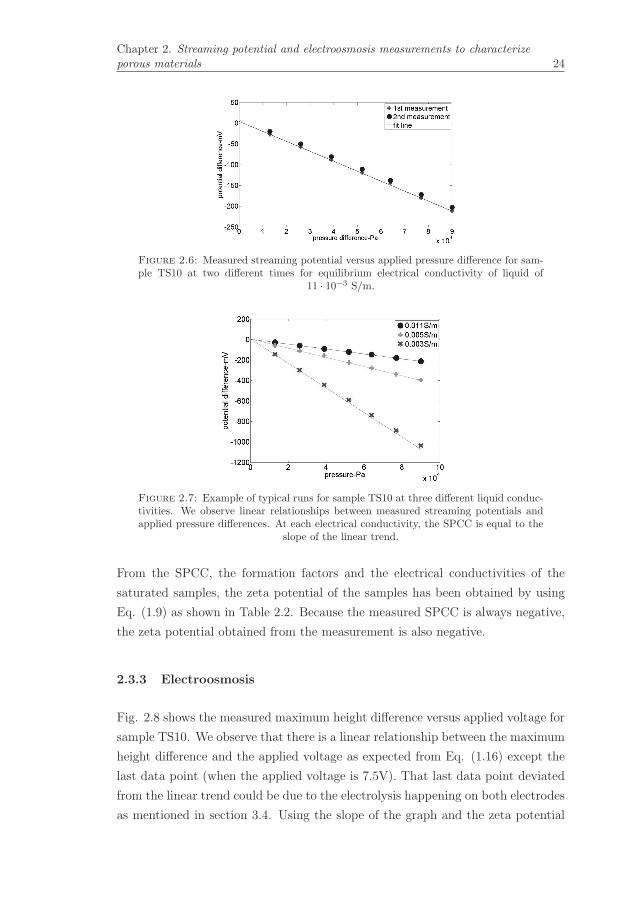
Chapter 2. Streaming potential and electroosmosis measurements to characterizeporous materials 24
Figure 2.6: Measured streaming potential versus applied pressure difference for sam-ple TS10 at two different times for equilibrium electrical conductivity of liquid of
11 · 10−3 S/m.
Figure 2.7: Example of typical runs for sample TS10 at three different liquid conduc-tivities. We observe linear relationships between measured streaming potentials andapplied pressure differences. At each electrical conductivity, the SPCC is equal to the
slope of the linear trend.
From the SPCC, the formation factors and the electrical conductivities of the
saturated samples, the zeta potential of the samples has been obtained by using
Eq. (1.9) as shown in Table 2.2. Because the measured SPCC is always negative,
the zeta potential obtained from the measurement is also negative.
2.3.3 Electroosmosis
Fig. 2.8 shows the measured maximum height difference versus applied voltage for
sample TS10. We observe that there is a linear relationship between the maximum
height difference and the applied voltage as expected from Eq. (1.16) except the
last data point (when the applied voltage is 7.5V). That last data point deviated
from the linear trend could be due to the electrolysis happening on both electrodes
as mentioned in section 3.4. Using the slope of the graph and the zeta potential

Chapter 2. Streaming potential and electroosmosis measurements to characterizeporous materials 25
Figure 2.8: Maximum height difference as a function of applied voltage for sampleTS10.
Table 2.2: Calculated parameters of the samples. In which ζ is zeta potential in mV,a is average pore radius in μm, N is the number of pores per cross sectional area of the
samples and ko is permeability of the samples in m2.
Sample TS10 TS20 TS40 TS140 TS250 TS500 Ssand
ζ -32.4 -5.2 -6.3 -12.5 -7.2 -9.1 13.7
a 2.3 3.2
N 775×103 482×103
ko 0.16×10⁻¹² 0.31×10⁻¹²
a from [58] 1.5 2.9 5.9 20.6 36.8 73.5
obtained from streaming potential measurement, we can estimate the average pore
size of the samples from eq. (1.16) as shown in Table 2.2.
Because of the limitation of applied voltage, the electroosmosis measurements are
only performed for sample TS10 and TS20. The height difference as a function
of time carried out for sample TS10 at possible maximum applied voltage of 6 V
is shown in Fig. 2.9. The graph has an exponential curve as expected from Eq.
(1.15). By using the exponential part of the graph, the response time in Eq. (1.13)
is obtained (see Fig. 2.10). From the calculated response time and parameters of
the samples, the number of pores on average can be determined by electroosmosis
measurements (see Table 2.2).
To check the validity of the pore size estimation, we use the relationship between
grain diameter and effective pore radius given by [58]
d = 2θa, (2.2)
where θ is the theta transform function that depends on parameters of the porous

Chapter 2. Streaming potential and electroosmosis measurements to characterizeporous materials 26
Figure 2.9: The dotted line is the experimental measurement of height difference asa function of time for sample TS10 at voltage of 6V (dotted line). The solid line is fit
through the data points.
Figure 2.10: The slope of the straight line is equal to the reciprocal of response time.
samples such as porosity, cementation exponent and formation factor of the sam-
ples. For the samples made of the monodisperse spherical particles arranged ran-
domly, θ is taken to be 3.4. From pore sizes determined by the electroosmosis
measurements, permeabilities of the samples are also calculated by the model of
[58] (see Table 2.2)
ko =a2φ3/2
8, (2.3)
where φ is porosity of the samples. From Table 2.2, we see that pore size estimated
from the electroosmosis measurement is in good agreement with that estimated
from the model of [58] and that in addition the calculated permeabilities are in
good agreement with measured ones in Table 2.1.
2.4 Conclusions
Streaming potential measurements have been performed for 7 unconsolidated sam-
ples fully saturated with a 10−3M NaCl solution to determine the zeta potentials.
Chapter 2. Streaming potential and electroosmosis measurements to characterizeporous materials 27
Because of the limitation of the voltage one can apply, we carry out the electroos-
mosis measurements for two smallest particle samples. This allows us to estimate
average pore sizes of the samples as well as the number of pores per cross sectional
area of porous media, which can not be determined by a method such as the image
analysis performed in [14] for very small pore porous media. The estimated pore
sizes and measured permeabilities have been compared to those calculated from
the model of [58] to check the validity of the measurements.
The comparison shows that the measured pore sizes are in good agreement with
the model of [58]. If the electroosmosis measurements can be improved e.g. by
using ion-exchange membranes or a large cross sectional area of the samples to
reduce the experimental time, this method can be effectively used to characterize
porous media by using simple measurements, in particular for very small pore
porous media that are relevant for application in the oil and gas industry.
Moreover, our measurements of streaming potential and electroosmosis also work
for the interface between a liquid and a polymeric material. The polymer may
be a more promising material for electroosmosis micropumps besides traditional
materials like silica particles. The zeta potential of the polymer material that we
use in this thesis is a little bit smaller than that of sands or sandstones.

Chapter 3
Permeability dependence of
streaming potential coupling
coefficients
3.1 Introduction
In chapter 2, streaming potential and electroosmosis measurements are carried
out to determine parameters such as the zeta potential, pore size, the number of
pores per cross sectional area of porous samples, porosity and permeability that
are very important for the seismoelectric effect [32]. However, how microstruc-
ture parameters of porous media such as permeability or porosity influence the
coupling between seismic wave and electromagnetic wave has not yet studied in
detail in the literature. In this chapter, we study the dependence of streaming
potential (seismoelectric effect at low frequency) on permeability of porous media.
In theory, the streaming potential coupling coefficient (SPCC) depends not only
on the fluids, pH, temperature and rock/fluid interface parameters but also on the
microstructure parameters of the rocks such as permeability of the rocks that par-
tially determines the effective conductivity of the rocks (see chapter 1). However,
in practice it is hard to show the permeability dependence of the SPCC because
of the variation of zeta potential from sample to sample.
Permeability dependence of the SPCC was experimentally studied by Jouniaux
and Pozzi [59] for sandstones and limestones in combination with a model to
quantify the effect of permeability on streaming potential. The authors presumed
the zeta potential to be the same for the same family of samples (for example,
29

Chapter 3. Permeability dependence of streaming potential coupling coefficients 30
Fontainebleau sandstones). However, the mineral composition is somehow differ-
ent from sample to sample even though they are taken from the same block of
rocks as shown by Pagoulatos [60] and therefore, the zeta potential that depends
on the mineral composition can vary. Perrier and Froidefond [61] also predicted
the permeability dependence of the SPCC for volcanic rocks using parameters ob-
tained in the laboratory such as the zeta potential and the rock resistivity with
two different fluid resistivities of 0.13 Ωm and 50 Ωm. Nevertheless, there is no ex-
perimental data to justify the theoretical results in [61]. Sprunt et al. [62] claimed
that the SPCC is experimentally independent of the permeability of the rock and
therefore that is contradiction to the results presented in [59] and [61].
Besides the conventional theory of streaming potential in which the zeta potential
is used, Revil and Mahardika [63] have recently presented a theory to calculate
the SPCC from the quasi-static volumetric charge density of the pore space that
depends on the permeability of rocks. Figure 3 in the work of Revil and Mahardika
[63] shows that at a given permeability, the quasi-static charge density may differ
by a factor of ten for different types of porous materials. Therefore, the SPCC
can be roughly predicted from the permeability with a deviation up to a factor
of ten. That means it could not explain the relationship between the SPCC and
the permeability in detail for a specific type of porous samples in a small range of
permeability.
In this chapter, we study permeability dependence of the SPCC including the
effects of the difference in the zeta potential between samples and the change of
surface conductance against electrolyte concentration. To do so, the ratio of the
SPCC and the zeta potential is used rather than the SPCC only. The results have
shown that the SPCC strongly depends on permeability of the samples for low
fluid electrical conductivity. However, when the fluid conductivity is larger than
a certain value that is determined by the mineral composition of the sample, the
SPCC is completely independent of permeability as explained in the theoretical
model.
This chapter has three sections. In the first we present the experimental setup and
measurements. The second section contains the experimental results, the compar-
ison between the experimental data and the theoretical model and discussion.
Conclusions are provided in the third section.

Chapter 3. Permeability dependence of streaming potential coupling coefficients 31
Table 3.1: Sample ID, mineral composition and microstructure parameters of the sam-ples. Symbols ko (in mD), φ (in %) , F (no units), α∞ (no units), ρs (in kg/m3) standfor permeability, porosity, formation factor, tortuosity and solid density, respectively.
Sample Mineral composition ko φ F α∞ ρsID
1 BereaUS1 Silica, Alumina, Ferric Oxide 120 14.5 19.0 2.8 2602Ferrous Oxide, Magnesium Oxide(www.bereasandstonecores.com)
2 BereaUS2 - 88 15.4 17.2 2.6 2576
3 BereaUS3 - 22 14.8 21.0 3.1 2711
4 BereaUS4 - 236 19.1 14.4 2.7 2617
5 BereaUS5 - 310 20.1 14.5 2.9 2514
6 BereaUS6 - 442 16.5 18.3 3.0 2541
7 DP50 Alumina and fused silica 2960 48.5 4.2 2.0 3546(see: www.tech-ceramics.co.uk)
8 DP46i - 4591 48.0 4.7 2.3 3559
9 DP217 - 370 45.4 4.5 2.0 3652
10 DP215 - 430 44.1 5.0 2.0 3453
11 DP43 - 4753 42.1 5.5 2.3 3373
12 DP172 - 5930 40.2 7.5 3.0 3258
3.2 Experiment
Streaming potential measurements have been performed on 12 consolidated sam-
ples (see Table 3.1). Natural samples numbered from 1 to 6 are Berea Sandstones
obtained from Berea Sandstone Petroleum Cores Company (USA). Artificial sam-
ples numbered from 7 to 12 are obtained from HP Technical Ceramics company
(UK). The mineral composition of all samples is also shown in the Table 3.1 (ac-
cording to the manufacturers).
For the measurements we use NaCl solutions with 7 different concentrations (4.0×10⁻⁴ M, 1.0 × 10⁻³ M, 2.5 × 10⁻³ M, 5.0 × 10⁻³ M, 1.0 × 10⁻² M, 2.0 × 10⁻² M
and 5.0× 10⁻² M). All measurements are carried out at room temperature (22 ±1◦C).
The details to measure the porosity, solid density, permeability and tortuosity of
consolidated samples are described in Appendix A. The experimental setup for
the measurement of the streaming potential is shown in Fig. 3.1. The core holder
contains a cylindrical sample of 55 mm in length and 25 mm in diameter. Each
sample is surrounded by a 4 mm thick silicone sleeve inside a conical stainless steel
cell and inserted into a stainless steel holder (see Fig. 3.2) to prevent flow along
the interface of the sample.

Chapter 3. Permeability dependence of streaming potential coupling coefficients 32
Figure 3.1: Experimental setup for streaming potential measurements. 1, Core holder;2, Ag/AgCl electrodes; 3, Pump; 4, Pressure transducer; 5, NaCl solution container.
Figure 3.2: Core holder. 1, sample; 2, silicone sleeve; 3, conical stainless steel cell; 4,stainless steel holder.
Figure 3.3: Streaming potential as a function of pressure difference for BereaUS5 atconcentration of 5.0× 10⁻² M. The inset shows an example of streaming potentials asa function of time at when pressure difference is switched from 0.72 bar to 0.94 bar.
The measurements are based on the technique mentioned in subsection 2.2.2 and
in [53]. The solution is circulated through the samples until the electrical conduc-
tivity and pH of the solution reaches a stable value. The pH values of equilibrium
solutions are in the range 6.0 to 7.5. To minimize CO2 uptake from the air that
leads to change of conductivity and pH of the solutions during the measurement,
the solution container is covered during experiment.
Electrical potential differences across the samples are then measured by a high
input impedance multimeter (Keithley Model 2700) connected to a computer.
Chapter 3. Permeability dependence of streaming potential coupling coefficients 33
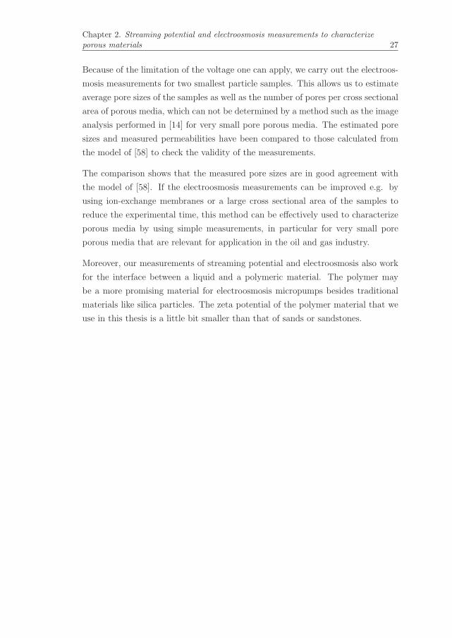
Figure 3.4: Impedance of the sample BereaUS5 as a function of frequency at differentconductivities of the electrolyte - 0.49, 0.69, 1.00 and 1.18 S/m, respectively.
The input resistance of the multimeter is larger than 10GΩ. The resistance of the
saturated samples is smaller than 200kΩ, which is low compared to input resistance
of the multimeter, therefore allowing accurate measurements of electric potentials.
The electrical potential difference at a given pressure difference fluctuates around
a specific value as shown in Fig. 3.3 (see the inset). The reason for that could be
partly due to periodic pulses of the pump when the piston switches its direction
after half a period. The values of the electrical potential difference are obtained
by a Labview program.
3.3 Results and discussion
3.3.1 Porosity, solid density, permeability and formation factor
Porosity, density and permeability of the samples are shown in Table 3.1 with
an error margin of 3%, 5% and 6% respectively. Porous sample resistances as a
function of frequency for example for the sample BereaUS5 are shown in Fig. 3.4
with 4 different conductivities - 0.49, 0.69, 1.00 and 1.18 S/m, respectively. The
resistances are seen to be frequency independent over the range 100 Hz to 100 kHz
and they are used to calculate the conductivity of the saturated samples, σS. The
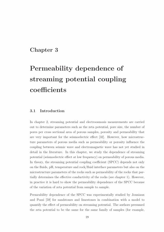
formation factor of the sample is obtained at 4 different conductivities as shown
in Fig. 3.5 and the final value is the average of all. Values of the formation factor
and corresponding tortuosity for all samples are also reported in Table 3.1 with
an error margin of 6% and 9%, respectively.
Chapter 3. Permeability dependence of streaming potential coupling coefficients 34
Figure 3.5: Formation factor of the sample BereaUS5 at different conductivities ofthe electrolyte - 0.49, 0.69, 1.00 and 1.18 S/m, respectively. The dash line is the average
value.
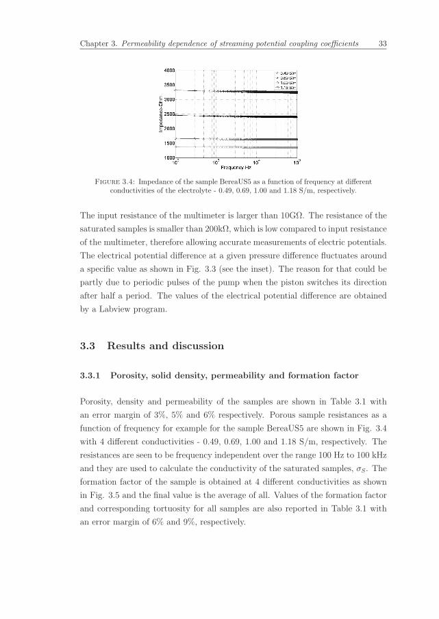
Figure 3.6: Coupling coefficient versus permeability for Berea samples at differentelectrolyte concentrations. The dash lines are the ones connecting the experimental
data points.
3.3.2 Streaming potential
The way used to collect the streaming potential is similar to that described in sub-
section 2.2.2 and in [53]. Fig. 3.3 shows streaming potentials as a function of time
at different pressure differences with a high concentration solution of 5.0×10⁻²M.
From Fig. 3.3, the streaming potential as a function of pressure difference and
therefore, the SPCC is obtained. Three measurements are performed for all sam-
ples with all solutions to find the SPCC. The SPCC for a given electrolyte concen-
tration is taken to be the average of the three values. Table 3.2 shows the SPCC for
all samples except for two samples DP43 and DP172 at electrolyte concentrations
of 2.0×10⁻²M and 5.0×10⁻²M. Because these samples are highly permeable, they
need a very large flow rate to generate measurable electric potential differences at
high concentration solutions. The maximum error of the SPCC is 15%.
Chapter 3. Permeability dependence of streaming potential coupling coefficients 35
Table 3.2: The coupling coefficients - CS(in mV/bar) for different electrolyte concen-trations of 4.0× 10⁻⁴ M, 10−3 M, 2.5× 10⁻³ M, 5.0× 10⁻³ M, 10−2 M, 2.0× 10⁻² M
and 5.0× 10⁻² M, respectively.
Sample ID 0.4 mM 1 mM 2.5 mM 5 mM 10 mM 20 mM 50 mM
BereaUS1 -65.0 -45.0 -22.0 -17.5 -9.7 -6.0 -2.8
BereaUS2 -72.0 -50.0 32.5 -20.3 -12.0 -7.0 -3.3
BereaUS3 -44.0 -33.0 -22.5 -17.8 -9.8 -6.0 -2.9
BereaUS4 -130.0 -75.0 -45.0 -27.5 -14.0 -8.4 -4.1
BereaUS5 -155.0 -100.0 -49.0 -34.0 -17.0 -9.2 -4.4
BereaUS6 -75.0 -50.0 -25.0 -16.0 -6.4 -3.9 -2.0
DP50 -260.0 -155.0 -80.0 -45.0 -19.0 -8.4 -3.0
DP46i -400.0 -230.0 -105.0 -53.0 -23.0 -12 -4.5
DP217 -280.0 -170.0 -85.0 -45.5 -24.0 -14.0 -6.0
DP215 -330.0 -190.0 -90.0 -56.0 -29.0 -12.0 -4.6
DP43 -390.0 -220.0 -78.0 -47.0 -22.0
DP172 -510.0 -300.0 -96.0 -50.0 -28.0
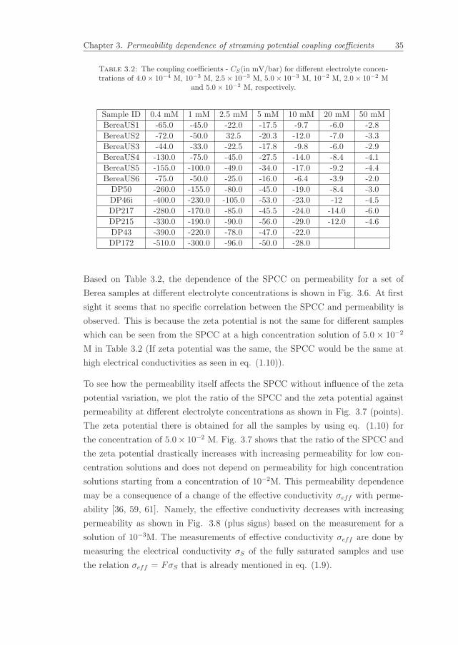
Based on Table 3.2, the dependence of the SPCC on permeability for a set of
Berea samples at different electrolyte concentrations is shown in Fig. 3.6. At first
sight it seems that no specific correlation between the SPCC and permeability is
observed. This is because the zeta potential is not the same for different samples
which can be seen from the SPCC at a high concentration solution of 5.0 × 10⁻²
M in Table 3.2 (If zeta potential was the same, the SPCC would be the same at
high electrical conductivities as seen in eq. (1.10)).
To see how the permeability itself affects the SPCC without influence of the zeta
potential variation, we plot the ratio of the SPCC and the zeta potential against
permeability at different electrolyte concentrations as shown in Fig. 3.7 (points).
The zeta potential there is obtained for all the samples by using eq. (1.10) for
the concentration of 5.0× 10⁻² M. Fig. 3.7 shows that the ratio of the SPCC and
the zeta potential drastically increases with increasing permeability for low con-
centration solutions and does not depend on permeability for high concentration
solutions starting from a concentration of 10−2M. This permeability dependence
may be a consequence of a change of the effective conductivity σeff with perme-
ability [36, 59, 61]. Namely, the effective conductivity decreases with increasing
permeability as shown in Fig. 3.8 (plus signs) based on the measurement for a
solution of 10−3M. The measurements of effective conductivity σeff are done by
measuring the electrical conductivity σS of the fully saturated samples and use
the relation σeff = FσS that is already mentioned in eq. (1.9).

Chapter 3. Permeability dependence of streaming potential coupling coefficients 36
Figure 3.7: The ratio of coupling coefficient and zeta potential versus permeabilityfor Berea samples at different concentrations. The solid lines are from the theoretical
model. The points are experimental data.
Figure 3.8: Effective conductivity versus permeability for Berea samples at 10−3Msolution.
That behavior can be theoretically explained by the effect of surface conductivity.
Effective conductivity σeff is given by [3]
σeff = σf + 2Σs
a, (3.1)
where σf is the fluid conductivity, Σs is the surface conductance and a is the pore
radius. According to [58], the permeability of the porous medium ko is related to
the pore size a by
ko =a2
8F, (3.2)

Chapter 3. Permeability dependence of streaming potential coupling coefficients 37
Table 3.3: The parameters used in eqs. (3.5 - 3.8) in the modeling of the surfaceconductance against electrolyte concentration.
Parameter Symbol Value Units
Temperature T 22 ◦CElectrolyte concentration Cf 4.0× 10⁻⁴ to 5.0× 10⁻² mol/L
Fluid pH pH 6.7 (-)Dielectric permittivity in vacuum ε0 8.854× 10⁻¹² F/m
Relative permittivity εr 80 (-)Boltzmann’s constant kb 1.381× 10⁻²³ J/KElementary charge e 1.602× 10⁻¹⁹ CAvogadro’s number N 6.022× 10²³ /mol
Ionic mobility of Na+ in solution βNa+ 5.20× 10⁻⁸ m2/s/VIonic mobility of H+ in solution βH+ 3.63× 10⁻⁷ m2/s/VIonic mobility of Cl− in solution βCl− 7.90× 10⁻⁸ m2/s/VIonic mobility of OH− in solution βOH− 2.05× 10⁻⁷ m2/s/VDisassociation constant of water Kw 9.214× 10⁻¹⁵ (-)Rock/fluid interface parameters
Surface site density Γs 10× 1018 sites/m2
Binding constant for Na+ adsorption KM 10−7.5 (-)Disassociation constant for K(−) 10−7.1 (-)
dehydrogenizationProton surface conductance cProt 12.10−28 for Bereas Sm2/site
4.10−28 for Ceramics(adjusted to fit data)
Ionic Stern-plane mobility βs 5.0×10⁻⁹ m2/s/V
where F is the formation factor of the porous medium. So eq. (3.1) can be
rewritten as
σeff = σf + 2Σs√8Fko
, (3.3)
and eq. (1.8) can be rewritten as
CS
ζ=
εrε0
η(σf + 2 Σs√8Fko
). (3.4)
According to the theory developed by [27], the zeta potential would decrease dras-
tically with increasing the electrolyte concentration. However, based on the three
measured values of the SPCC for the Berea samples in Table 3.2 at the high elec-
trolyte concentrations of 10−2M, 2.0×10⁻²M and 5.0×10⁻²M, the zeta potential of
the samples at three corresponding concentrations is calculated by using eq. (1.10).
The results show that the calculated zeta potential only slightly decreases with
increasing the concentration and can be considered as constant over the studied
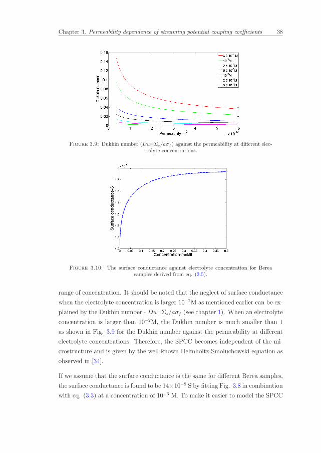
Chapter 3. Permeability dependence of streaming potential coupling coefficients 38
Figure 3.9: Dukhin number (Du=Σs/aσf ) against the permeability at different elec-trolyte concentrations.
Figure 3.10: The surface conductance against electrolyte concentration for Bereasamples derived from eq. (3.5).
range of concentration. It should be noted that the neglect of surface conductance
when the electrolyte concentration is larger 10−2M as mentioned earlier can be ex-
plained by the Dukhin number - Du=Σs/aσf (see chapter 1). When an electrolyte
concentration is larger than 10−2M, the Dukhin number is much smaller than 1
as shown in Fig. 3.9 for the Dukhin number against the permeability at different
electrolyte concentrations. Therefore, the SPCC becomes independent of the mi-
crostructure and is given by the well-known Helmholtz-Smoluchowski equation as
observed in [34].
If we assume that the surface conductance is the same for different Berea samples,
the surface conductance is found to be 14×10−9 S by fitting Fig. 3.8 in combination
with eq. (3.3) at a concentration of 10−3 M. To make it easier to model the SPCC

Chapter 3. Permeability dependence of streaming potential coupling coefficients 39
as a function of permeability, the formation factor F in eq. (3.3) and eq. (3.4) is
taken as a constant averaged over all the samples.
To take into account the change of the surface conductance with the electrolyte
concentration, we use the formulas described in [27, 64] in which the surface con-
ductance is given by
Σs = ΣEDL + ΣStern + ΣProt, (3.5)
where ΣEDL, ΣStern and ΣProt are the contributions to the surface conductivity
from ionic conduction in the EDL, in the Stern layer and associated with proton
transfer, respectively. The above formula is developed for 1:1 electrolyte of the
aqueous NaCl solution and quartz, it still works for other porous materials such
as Fontainebleau, Stainton, St.Bees sandstones or Carbonates and etc (see [27] for
more details).
Where
ΣEDL = R{[(βNa+Cf + βH+10−pH)((S(
10−pH +KMCf
2eΓsK(−)))−1/3 − 1)]
+ [(βCl−Cf + βOH−10pH−pKw)((S(10−pH +KMCf
2eΓsK(−)))+1/3 − 1)]}
(3.6)
and
ΣStern =eβsΓsKMCf
10−pH +K(−) +KMCf
, (3.7)
and
ΣProt = cProtΓs, (3.8)
in which R=√
2×10³εrε0kbTNCf+10−pH
and S=√8× 10³εrε0kbTN(Cf + 10−pH + 10pH−pKw). Where βNa+, βH+, βCl− and
βOH− are the ionic mobilities of Na+, H+, Cl− and OH−, respectively. Γs is the
surface site density of the solid surface. KM is the binding constant for Na+
adsorption. K(−) is the disassociation constant for dehydrogenization of silanol.
cProt is the proton surface conductance. βs is the ionic Stern-plane mobility. Kw
is the Disassociation constant of water. N is the Avogadro’s number (see [27] for
more details).
The parameters used in eqs. (3.5 - 3.8) are taken from [27] except the proton
surface conductance and are shown in Table 3.3. The proton surface conductance
has been adjusted to fit data based on the surface conductance of 14× 10−9 S at
10−3 M concentration and shown in Table 3.3. Fig. 3.10 shows the change of the
surface conductance over electrolyte concentration with the parameters shown in
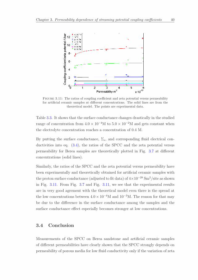
Chapter 3. Permeability dependence of streaming potential coupling coefficients 40
Figure 3.11: The ratios of coupling coefficient and zeta potential versus permeabilityfor artificial ceramic samples at different concentrations. The solid lines are from the
theoretical model. The points are experimental data.
Table 3.3. It shows that the surface conductance changes drastically in the studied
range of concentration from 4.0× 10⁻⁴M to 5.0× 10⁻²M and gets constant when
the electrolyte concentration reaches a concentration of 0.4 M.
By putting the surface conductance, Σs, and corresponding fluid electrical con-
ductivities into eq. (3.4), the ratios of the SPCC and the zeta potential versus
permeability for Berea samples are theoretically plotted in Fig. 3.7 at different
concentrations (solid lines).
Similarly, the ratios of the SPCC and the zeta potential versus permeability have
been experimentally and theoretically obtained for artificial ceramic samples with
the proton surface conductance (adjusted to fit data) of 4×10⁻²⁸ Sm2/site as shown
in Fig. 3.11. From Fig. 3.7 and Fig. 3.11, we see that the experimental results
are in very good agrement with the theoretical model even there is the spread at
the low concentrations between 4.0× 10⁻⁴M and 10−3M. The reason for that may
be due to the difference in the surface conductance among the samples and the
surface conductance effect especially becomes stronger at low concentrations.
3.4 Conclusion
Measurements of the SPCC on Berea sandstone and artificial ceramic samples
of different permeabilities have clearly shown that the SPCC strongly depends on
permeability of porous media for low fluid conductivity only if the variation of zeta
Chapter 3. Permeability dependence of streaming potential coupling coefficients 41
potential between the samples is taken into account. When the fluid conductivity
is larger than 0.13 S/m (NaCl concentration is higher than 0.01 M), the SPCC
is completely independent of permeability. We use a theoretical model to explain
the relationship between the SPCC and permeability. In the model we take into
account the change of surface conductivity over electrolyte concentration and the
variation of zeta potential from sample to sample. Consequently, the modeled
results are in better agrement with the experimental results for two sets of samples.
This study demonstrates that the permeability of the reservoir rock for liquid is
an important parameter influencing the SPCC for low conductivity liquid. In
regions where sea water (around 5 S/m in conductivity) is dominant, the SPCC
is probably not affected by changes of permeability because the ratio of surface
conductivity to fluid conductivity is very low.


Chapter 4
Examination of a theoretical
model of streaming potential
coupling coefficient
4.1 Introduction
Characterization of porous media and permeability dependence of the streaming
potential coupling coefficient (SPCC) are studied in chapter 2 and chapter 3,
respectively. In those chapters, the SPCC is experimentally measured and the
zeta potential is deduced from that with knowledge of the electrical conductivity,
viscosity and electrical permittivity of the fluid. That is the most commonly used
approach to obtain the SPCC and the zeta potential of electrolyte saturated rocks.
Glover et al. [27] developed a theoretical model to calculate the zeta potential
and the SPCC of reservoir rocks and other porous media. By using reasonable
values of input parameters that are supported by independent measurements or
theory, Glover et al. [27] have obtained and compared the theoretical results
to an experimental data set of 290 SPCC measurements and 269 zeta potential
measurements using data from 29 publications. The comparison shows that the
theoretical model can reproduce the main features of the experimental data.
However, the experimental data set was collected from different sources that may
lead to a dissimilarity in fluid conductivity, in pH of pore fluid (a big range of pH
from 5.5 to 11), in temperature and sample compositions. Some microstructure pa-
rameters that are needed to model were also not given in the original publications.
The zeta potential and surface conductance themselves may be also different from
43
Chapter 4. Examination of a theoretical model of streaming potential couplingcoefficient 44
sample to sample [65]. Therefore, All those dissimilarities may cause the observed
deviations.
In this chapter we want to examine how well the model work for 20 consolidated
samples with 7 different concentrations of a NaCl solution and 9 different tem-
peratures. To do so, firstly the SPCC and the zeta potential are experimentally
measured as a function of the electrolyte concentration and temperature. After-
wards the model is used by taking fluid parameters, rock-fluid interface parameters
already provided in [27] and rock microstructure parameters (porosity, permeabil-
ity and formation factor) measured by ourself for all samples. The proton surface
conductance is adjusted to fit the experimental data. The comparisons are carried
out for each sample.
For electrolyte concentration dependence of the SPCC, the comparison shows that
the theoretical model is not in agreement with the experimental data, especially in
low concentration range. However, if the zeta potential is considered to be constant
over electrolyte concentration at fixed temperature the model fits the experimental
data very well in a whole range of concentration. This leads to the suggestion that
the formula of the zeta potential against electrolyte concentration in the model
needs to be adjusted accordingly. Beside the model given in [27], we also use other
empirical models from Pride and Morgan [66], Vinogradov et al. [67], Jaafar et al.
[68] and Jouniaux and Ishido [69] to predict the SPCC as a function of electrolyte
concentration. But none of them can fit experimental data at low electrolyte
concentration. For temperature dependence of the SPCC, we implement a zeta
potential offset to the model which improves the fit to experimental data. The
comparison shows that the theoretical model does not fit the experimental data
well but it can show the increase of the SPCC with increasing temperature as
measured.
This chapter includes five sections. Section 4.2 describes the theoretical back-
ground of streaming potential including the calculation of the Stern potential, the
zeta potential, fluid relative electric permittivity, fluid viscosity, fluid electrical
conductivity and disassociation constant of water. Section 4.3 presents the exper-
imental measurements. Section 4.4 contains the experimental results, discussion
and comparisons between the experimental data and the results of the theoretical
model. Conclusions are provided in Section 4.5.
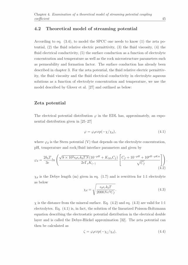
Chapter 4. Examination of a theoretical model of streaming potential couplingcoefficient 45
4.2 Theoretical model of streaming potential
According to eq. (3.4), to model the SPCC one needs to know (1) the zeta po-
tential, (2) the fluid relative electric permittivity, (3) the fluid viscosity, (4) the
fluid electrical conductivity, (5) the surface conduction as a function of electrolyte
concentration and temperature as well as the rock microstructure parameters such
as permeability and formation factor. The surface conduction has already been
described in chapter 3. For the zeta potential, the fluid relative electric permittiv-
ity, the fluid viscosity and the fluid electrical conductivity in electrolyte aqueous
solutions as a function of electrolyte concentration and temperature, we use the
model described by Glover et al. [27] and outlined as below:
Zeta potential
The electrical potential distribution ϕ in the EDL has, approximately, an expo-
nential distribution given in [25–27]
ϕ = ϕdexp(−χ/χd), (4.1)
where ϕd is the Stern potential (V) that depends on the electrolyte concentration,
pH, temperature and rock/fluid interface parameters and given by
ϕd =2kbT
3eln
(√8× 10³ε0εrkbTN(10−pH +KMeCf )
2eΓsK(−)
[Cf + 10−pH + 10pH−pKw√
Cf
]).
(4.2)
χd is the Debye length (m) given in eq. (1.7) and is rewritten for 1:1 electrolyte
as below
χd =
√ε0εrkbT
2000Ne2Cf
. (4.3)
χ is the distance from the mineral surface. Eq. (4.2) and eq. (4.3) are valid for 1:1
electrolytes. Eq. (4.1) is, in fact, the solution of the linearized Poisson-Boltzmann
equation describing the electrostatic potential distribution in the electrical double
layer and is called the Debye-Huckel approximation [32]. The zeta potential can
then be calculated as
ζ = ϕdexp(−χζ/χd), (4.4)
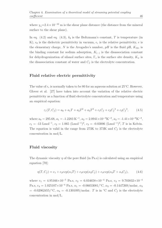
Chapter 4. Examination of a theoretical model of streaming potential couplingcoefficient 46
where χζ=2.4×10⁻¹⁰ m is the shear plane distance (the distance from the mineral
surface to the shear plane).
In eq. (4.2) and eq. (4.3), kb is the Boltzmann’s constant, T is temperature (in
K), ε0 is the dielectric permittivity in vacuum, εr is the relative permittivity, e is
the elementary charge, N is the Avogadro’s number, pH is the fluid pH, KMe is
the binding constant for sodium adsorption, K(−) is the disassociation constant
for dehydrogenization of silanol surface sites, Γs is the surface site density, Kw is
the disassociation constant of water and Cf is the electrolyte concentration.
Fluid relative electric permittivity
The value of εr is normally taken to be 80 for an aqueous solution at 25◦C. However,
Glover et al. [27] have taken into account the variation of the relative electric
permittivity as a function of fluid electrolyte concentration and temperature using
an empirical equation:
εr(T,Cf ) = a0 + a1T + a2T2 + a3T
3 + c1Cf + c2Cf2 + c3Cf
3, (4.5)
where a0 = 295.68, a1 = -1.2283 K−1, a2 = 2.0941×10⁻³K−2, a3 = -1.41×10⁻⁶K−3,
c1 = -13 Lmol−1, c2 = 1.065 (Lmol−1)2, c3 = -0.03006 (Lmol−1)3, T is in Kelvin.
The equation is valid in the range from 273K to 373K and Cf is the electrolyte
concentration in mol/L.
Fluid viscosity
The dynamic viscosity η of the pore fluid (in Pa.s) is calculated using an empirical
equation [70]:
η(T,Cf ) = e1 + e2exp(α1T ) + e3exp(α2Cf ) + e4exp(α3T + α4Cf ), (4.6)
where e1 = 4.95166×10⁻⁵ Pa.s, e2 = 6.034658×10⁻⁴ Pa.s, e3 = 9.703832×10⁻⁴
Pa.s, e4 = 1.025107×10⁻⁴ Pa.s, α1 = -0.06653081/◦C, α2 = -0.1447269/molar, α3
= -0.02062455/◦C, α4 = -0.1301095/molar. T is in ◦C and Cf is the electrolyte
concentration in mol/L.

Chapter 4. Examination of a theoretical model of streaming potential couplingcoefficient 47
Fluid electrical conductivity
The fluid electrical conductivity (in S/m) is given in [27, 71] as a function of fluid
concentration and temperature
σf (T,Cf ) = (d1 + d2T + d3T2)Cf − (
d4 + d5T
1 + d6√Cf
)Cf3/2, (4.7)
where d1 = 5.6 (S.L/m.mol), d2 = 0.27 (S.L/m.mol)/◦C, d3 = −1.51 × 10⁻⁴
(S.L/m.mol)/◦C2, d4 = 2.36 (S/m/(mol/L)3/2), d5 = 0.099 (S/m/(mol/L)3/2/◦C),
d6 = 0.214 ((mol/L)−1/2). T is in ◦C and Cf is the electrolyte concentration in
mol/L.
Disassociation constant
This parameter defines the fluid pH which is required to calculate the Stern po-
tential and the surface conductance. The value of Kw varies with temperature and
is approximately in the range of 0◦C to 100◦C as follows [54]
Kw = 6.9978×10⁻¹⁶+5.0178×10⁻¹⁶T−2.4434×10⁻¹⁷T 2+7.1948×10⁻¹⁹T 3 (4.8)
where T is in ◦C.
Indeed, the fluid pH is also defined by the reaction of water with carbon dioxide
from the air which generates bicarbonate (HCO3) and hydrogen ions (H+) [27].
This leads to that water exposed to air is slightly acidic. In the model, one needs
to know the pH to calculate the concentrations of hydrogen ions (10−pH) and
hydroxyl ions (10pH−pKw) in the fluid. The pH values required to model is directly
measured by a pH meter.
4.3 Experiments
Streaming potential measurements have been performed on 20 consolidated sam-
ples (55 mm in length and 25 mm in diameter as shown in Fig. 4.1) including
both natural and artificial samples from different sources. Beside 12 consolidated
samples used in chapter 3 for the study of permeability dependence of the SPCC
(see Table 3.1), we use 8 more samples for the experimental examination of the
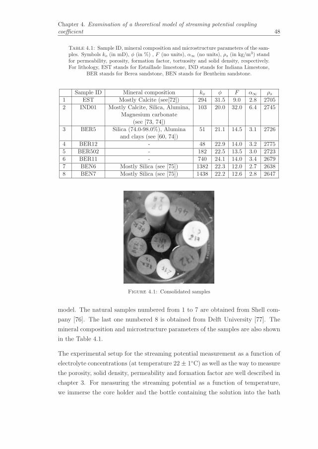
Chapter 4. Examination of a theoretical model of streaming potential couplingcoefficient 48
Table 4.1: Sample ID, mineral composition and microstructure parameters of the sam-ples. Symbols ko (in mD), φ (in %) , F (no units), α∞ (no units), ρs (in kg/m3) standfor permeability, porosity, formation factor, tortuosity and solid density, respectively.For lithology, EST stands for Estaillade limestone, IND stands for Indiana Limestone,
BER stands for Berea sandstone, BEN stands for Bentheim sandstone.
Sample ID Mineral composition ko φ F α∞ ρs1 EST Mostly Calcite (see[72]) 294 31.5 9.0 2.8 2705
2 IND01 Mostly Calcite, Silica, Alumina, 103 20.0 32.0 6.4 2745Magnesium carbonate
(see [73, 74])
3 BER5 Silica (74.0-98.0%), Alumina 51 21.1 14.5 3.1 2726and clays (see [60, 74])
4 BER12 - 48 22.9 14.0 3.2 2775
5 BER502 - 182 22.5 13.5 3.0 2723
6 BER11 - 740 24.1 14.0 3.4 2679
7 BEN6 Mostly Silica (see [75]) 1382 22.3 12.0 2.7 2638
8 BEN7 Mostly Silica (see [75]) 1438 22.2 12.6 2.8 2647
Figure 4.1: Consolidated samples
model. The natural samples numbered from 1 to 7 are obtained from Shell com-
pany [76]. The last one numbered 8 is obtained from Delft University [77]. The
mineral composition and microstructure parameters of the samples are also shown
in the Table 4.1.
The experimental setup for the streaming potential measurement as a function of
electrolyte concentrations (at temperature 22 ± 1◦C) as well as the way to measure
the porosity, solid density, permeability and formation factor are well described in
chapter 3. For measuring the streaming potential as a function of temperature,
we immerse the core holder and the bottle containing the solution into the bath
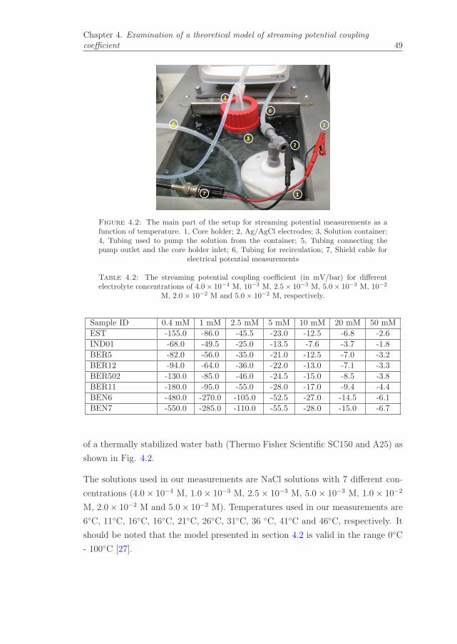
Chapter 4. Examination of a theoretical model of streaming potential couplingcoefficient 49
Figure 4.2: The main part of the setup for streaming potential measurements as afunction of temperature. 1, Core holder; 2, Ag/AgCl electrodes; 3, Solution container;4, Tubing used to pump the solution from the container; 5, Tubing connecting thepump outlet and the core holder inlet; 6, Tubing for recirculation; 7, Shield cable for
electrical potential measurements
Table 4.2: The streaming potential coupling coefficient (in mV/bar) for differentelectrolyte concentrations of 4.0× 10⁻⁴ M, 10−3 M, 2.5× 10⁻³ M, 5.0× 10⁻³ M, 10−2
M, 2.0× 10⁻² M and 5.0× 10⁻² M, respectively.
Sample ID 0.4 mM 1 mM 2.5 mM 5 mM 10 mM 20 mM 50 mM
EST -155.0 -86.0 -45.5 -23.0 -12.5 -6.8 -2.6
IND01 -68.0 -49.5 -25.0 -13.5 -7.6 -3.7 -1.8
BER5 -82.0 -56.0 -35.0 -21.0 -12.5 -7.0 -3.2
BER12 -94.0 -64.0 -36.0 -22.0 -13.0 -7.1 -3.3
BER502 -130.0 -85.0 -46.0 -24.5 -15.0 -8.5 -3.8
BER11 -180.0 -95.0 -55.0 -28.0 -17.0 -9.4 -4.4
BEN6 -480.0 -270.0 -105.0 -52.5 -27.0 -14.5 -6.1
BEN7 -550.0 -285.0 -110.0 -55.5 -28.0 -15.0 -6.7
of a thermally stabilized water bath (Thermo Fisher Scientific SC150 and A25) as
shown in Fig. 4.2.
The solutions used in our measurements are NaCl solutions with 7 different con-
centrations (4.0× 10⁻⁴ M, 1.0× 10⁻³ M, 2.5× 10⁻³ M, 5.0× 10⁻³ M, 1.0× 10⁻²
M, 2.0× 10⁻² M and 5.0× 10⁻² M). Temperatures used in our measurements are
6◦C, 11◦C, 16◦C, 16◦C, 21◦C, 26◦C, 31◦C, 36 ◦C, 41◦C and 46◦C, respectively. It
should be noted that the model presented in section 4.2 is valid in the range 0◦C
- 100◦C [27].
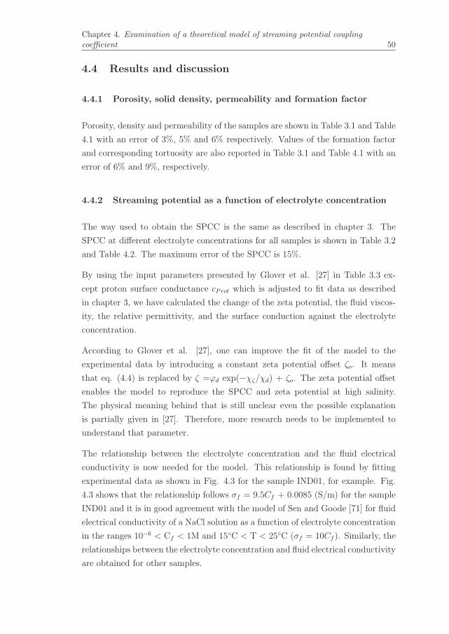
Chapter 4. Examination of a theoretical model of streaming potential couplingcoefficient 50
4.4 Results and discussion
4.4.1 Porosity, solid density, permeability and formation factor
Porosity, density and permeability of the samples are shown in Table 3.1 and Table
4.1 with an error of 3%, 5% and 6% respectively. Values of the formation factor
and corresponding tortuosity are also reported in Table 3.1 and Table 4.1 with an
error of 6% and 9%, respectively.
4.4.2 Streaming potential as a function of electrolyte concentration
The way used to obtain the SPCC is the same as described in chapter 3. The
SPCC at different electrolyte concentrations for all samples is shown in Table 3.2
and Table 4.2. The maximum error of the SPCC is 15%.
By using the input parameters presented by Glover et al. [27] in Table 3.3 ex-
cept proton surface conductance cProt which is adjusted to fit data as described
in chapter 3, we have calculated the change of the zeta potential, the fluid viscos-
ity, the relative permittivity, and the surface conduction against the electrolyte
concentration.
According to Glover et al. [27], one can improve the fit of the model to the
experimental data by introducing a constant zeta potential offset ζo. It means
that eq. (4.4) is replaced by ζ =ϕd exp(−χζ/χd) + ζo. The zeta potential offset
enables the model to reproduce the SPCC and zeta potential at high salinity.
The physical meaning behind that is still unclear even the possible explanation
is partially given in [27]. Therefore, more research needs to be implemented to
understand that parameter.
The relationship between the electrolyte concentration and the fluid electrical
conductivity is now needed for the model. This relationship is found by fitting
experimental data as shown in Fig. 4.3 for the sample IND01, for example. Fig.
4.3 shows that the relationship follows σf = 9.5Cf + 0.0085 (S/m) for the sample
IND01 and it is in good agreement with the model of Sen and Goode [71] for fluid
electrical conductivity of a NaCl solution as a function of electrolyte concentration
in the ranges 10−6 < Cf < 1M and 15◦C < T < 25◦C (σf = 10Cf ). Similarly, the
relationships between the electrolyte concentration and fluid electrical conductivity
are obtained for other samples.
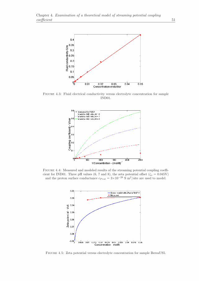
Chapter 4. Examination of a theoretical model of streaming potential couplingcoefficient 51
Figure 4.3: Fluid electrical conductivity versus electrolyte concentration for sampleIND01.
Figure 4.4: Measured and modeled results of the streaming potential coupling coeffi-cient for IND01. Three pH values (6, 7 and 8), the zeta potential offset (ζo = 0.045V)and the proton surface conductance cProt = 3×10⁻²⁸ S m2/site are used to model.
Figure 4.5: Zeta potential versus electrolyte concentration for sample BereaUS5.
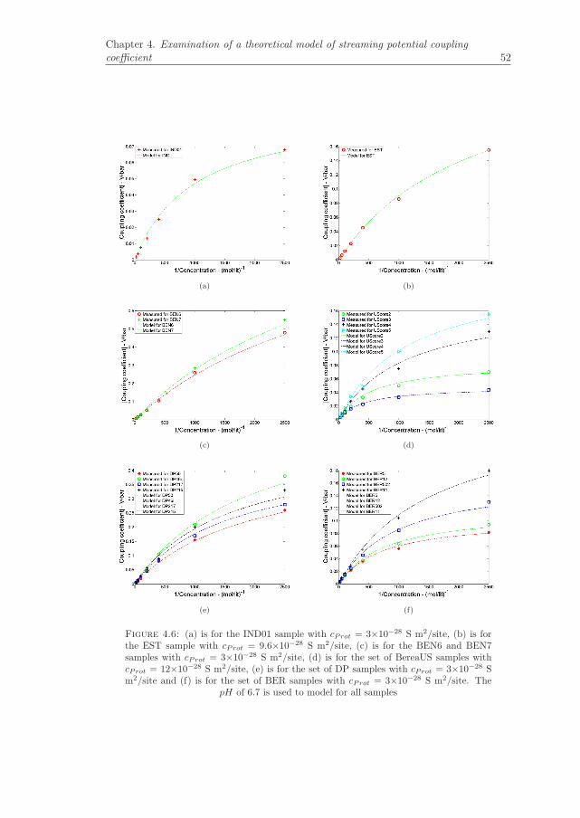
Chapter 4. Examination of a theoretical model of streaming potential couplingcoefficient 52
(a) (b)
(c) (d)
(e) (f)
Figure 4.6: (a) is for the IND01 sample with cProt = 3×10⁻²⁸ S m2/site, (b) is forthe EST sample with cProt = 9.6×10⁻²⁸ S m2/site, (c) is for the BEN6 and BEN7samples with cProt = 3×10⁻²⁸ S m2/site, (d) is for the set of BereaUS samples withcProt = 12×10−28 S m2/site, (e) is for the set of DP samples with cProt = 3×10⁻²⁸ Sm2/site and (f) is for the set of BER samples with cProt = 3×10⁻²⁸ S m2/site. The
pH of 6.7 is used to model for all samples

Chapter 4. Examination of a theoretical model of streaming potential couplingcoefficient 53
All data is now sufficient to model the SPCC as a function of electrolyte concen-
tration from eq. (3.4) in combination with input parameters given by [27] in Table
3.3. Fig. 4.4 shows the experimental and modeled results of the SPCC for sample
IND01. The modeled result is implemented for three values of pH (pH = 6, 7 and
8) with the zeta potential offset ζo = 0.045V and the proton surface conductance
cProt = 3×10⁻²⁸ S m2/site. Fig. 4.4 shows that the model of the SPCC against
the electrolyte concentration is very sensitive to the pH of the fluid as expected in
[27]. The model is not in good agreement with the experimental result in partic-
ular at a low concentration where the deviation of SPCC from experimental data
increases.
The deviation between the modeled and experimental results could arise from the
formula proposed to calculate the zeta potential in eqs. (4.2 - 4.4). According
to the model, the zeta potential in magnitude would decrease drastically with
increasing the electrolyte concentration as shown in Fig. 4.5 (the solid line).
However, based on the three measured values of the SPCC for all samples in Table
4.2 at the high electrolyte concentrations of 10−2M, 2×10⁻²M and 5×10⁻²M, the
zeta potential at those corresponding concentrations is calculated by using eq.
(1.10) as shown in Fig. 4.5 (the dashed line) for sample BereaUS5, for example. It
is worthwhile noting that the surface conductance is neglected when the electrolyte
concentration is higher than 10−2M as mentioned in chapter 3. It is obvious
that the measured zeta potential slightly decreases with increasing concentration
and can be roughly considered constant over the studied range of the electrolyte
concentration. Similarly, the zeta potentials are experimentally obtained for other
samples.
We therefore assume the zeta potential to be constant over the electrolyte concen-
tration and that is also inferred from the collected experimental data presented in
[69]. The dependence of the SPCC on the electrolyte concentration for all samples
with corresponding proton surface conductance is experimentally and theoretically
shown in Fig. 4.6 in which Fig. 4.6(a) is for the IND01 sample, Fig. 4.6(b) is
for the EST sample, Fig.4.6(c) is for the BEN6 and BEN7 samples, Fig. 4.6(d)
is for the set of BereaUS samples, Fig. 4.6(e) is for the set of DP samples and
Fig. 4.6(f) is for the set of BER samples, respectively. To avoid the overlap of
the experimental data shown in Fig. 4.6(d) and Fig. 4.6(e), we only show the
experimental graphs for four out of six samples for the sets of BereaUS and DP
samples, respectively. All theoretical results are carried out for pH of 6.7 because
this value is the average of measured values (between 6 and 7.5). For reasons of
clarity, the SPCC is plotted against the reverse of the electrolyte concentration
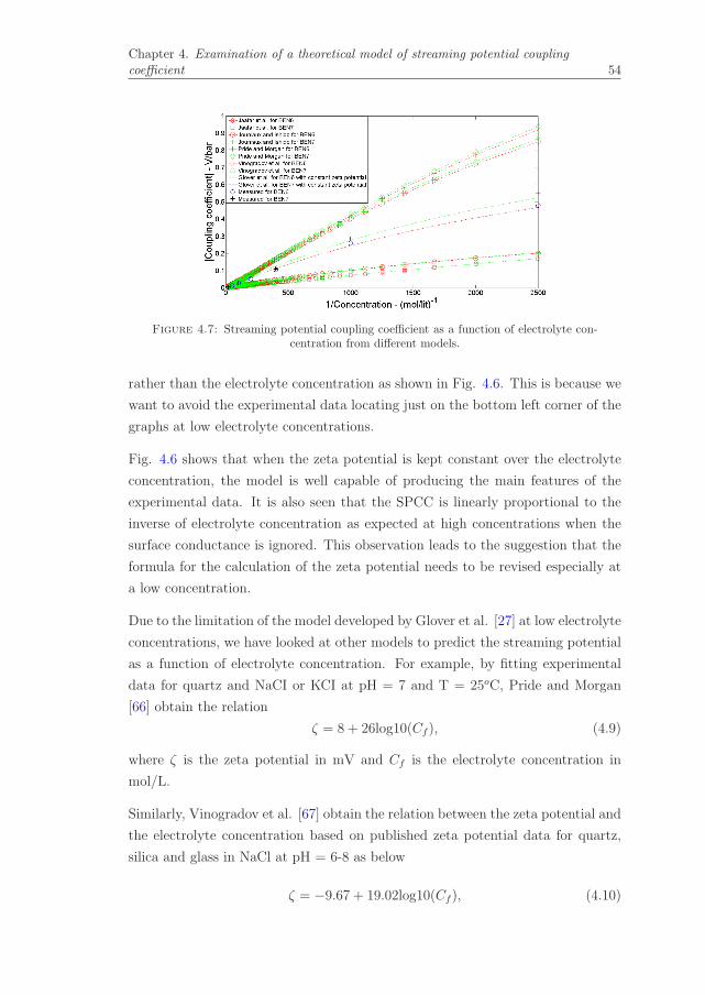
Chapter 4. Examination of a theoretical model of streaming potential couplingcoefficient 54
Figure 4.7: Streaming potential coupling coefficient as a function of electrolyte con-centration from different models.
rather than the electrolyte concentration as shown in Fig. 4.6. This is because we
want to avoid the experimental data locating just on the bottom left corner of the
graphs at low electrolyte concentrations.
Fig. 4.6 shows that when the zeta potential is kept constant over the electrolyte
concentration, the model is well capable of producing the main features of the
experimental data. It is also seen that the SPCC is linearly proportional to the
inverse of electrolyte concentration as expected at high concentrations when the
surface conductance is ignored. This observation leads to the suggestion that the
formula for the calculation of the zeta potential needs to be revised especially at
a low concentration.
Due to the limitation of the model developed by Glover et al. [27] at low electrolyte
concentrations, we have looked at other models to predict the streaming potential
as a function of electrolyte concentration. For example, by fitting experimental
data for quartz and NaCI or KCI at pH = 7 and T = 25oC, Pride and Morgan
[66] obtain the relation
ζ = 8 + 26log10(Cf ), (4.9)
where ζ is the zeta potential in mV and Cf is the electrolyte concentration in
mol/L.
Similarly, Vinogradov et al. [67] obtain the relation between the zeta potential and
the electrolyte concentration based on published zeta potential data for quartz,
silica and glass in NaCl at pH = 6-8 as below
ζ = −9.67 + 19.02log10(Cf ), (4.10)

Chapter 4. Examination of a theoretical model of streaming potential couplingcoefficient 55
By fitting experimental data collected for sandstone, sand, silica nanochannels,
Stainton, and Fountainbleau with electrolytes of NaCl and KCl at pH = 6-8, Jaafar
et al. [68] obtain an empirical expression between the SPCC and the electrolyte
concentration
CS = −1.36Cf−0.9123, (4.11)
where CS is expressed in mV MPa−1.
Jouniaux and Ishido [69] obtain the other relation to predict the SPCC from fluid
conductivity based on numerous measurements of the streaming potential on sand
with NaCl at pH = 7-8 which have been published
CS =−1.2× 10⁻⁸
σf
, (4.12)
where σf is the fluid electrical conductivity and CS is in V Pa−1.
Putting eq. (4.9) and eq. (4.10) into eq. (3.4), the SPCC as a function of
electrolyte concentration (CS-Cf ) is obtained for the models of Pride and Morgan
and Vinogradov et al., respectively. From eq. (4.11), CS-Cf is directly obtained for
model of Jaafar et al. To plot CS-Cf for the model of Jouniaux and Ishido from eq.
(4.12), the fluid electrical conductivity as a function of electrolyte concentration
obtained by fitting experimental data as shown in Fig. 4.3 is used. The prediction
of the SPCC as a function of electrolyte concentration from all four empirical
models is shown in Fig. 4.7.
Because all empirical models are mostly obtained for the silica based samples,
experimental data for Bentheim sandstone mainly made up by silica (see Table
4.1) is used for the comparison as shown in Fig. 4.7. The prediction from the model
of Glover et al. with the adjustment of the constant zeta potential for Bentheim
sandstone shown Fig.4.6(c) is also repeated in Fig. 4.7. The comparison shows
that the SPCC from all models converges and agrees with the experimental data at
high electrolyte concentrations. However, at low concentrations (smaller than 10−2
M) the SPCC diverges from each other and does not agree with experimental data.
Theoretical values from the models of Pride and Morgan as well as Vinogradov et
al. are approximately twice as high as experimental values (see upper curves in
Fig. 4.7). While theoretical values from the models of Jouniaux and Ishido and
Jaafar et al. are approximately half of the experimental values (see lower curves
in Fig. 4.7). Therefore, all four empirical models fail to predict the SPCC as
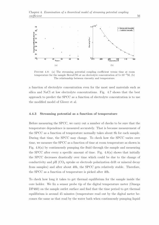
Chapter 4. Examination of a theoretical model of streaming potential couplingcoefficient 56
(a) (b)
Figure 4.8: (a) The streaming potential coupling coefficient versus time at roomtemperature for the sample BereaUS5 at an electrolyte concentration of 5×10⁻³M, (b)
The relationship between viscosity and temperature.
a function of electrolyte concentration even for the most used materials such as
silica and NaCl at low electrolyte concentrations. Fig. 4.7 shows that the best
approach to predict the SPCC as a function of electrolyte concentration is to use
the modified model of Glover et al.
4.4.3 Streaming potential as a function of temperature
Before measuring the SPCC, we carry out a number of checks to be sure that the
temperature dependence is measured accurately. That is because measurement of
the SPCC as a function of temperature normally takes about 8h for each sample.
During that time, the SPCC may change. To check how the SPCC varies over
time, we measure the SPCC as a function of time at room temperature as shown in
Fig. 4.8(a) by continuously pumping the fluid through the sample and measuring
the SPCC after every a specific amount of time. Fig. 4.8(a) shows that initially
the SPCC decreases drastically over time which could be due to the change of
conductivity and pH (CO2 uptake or electrode polarization drift or mineral decay
from samples) and after about 40h, the SPCC gets relatively stable. Therefore,
the SPCC as a function of temperature is picked after 40h.
To check how long it takes to get thermal equilibrium for the sample inside the
core holder. We fix a sensor probe tip of the digital temperature meter (Omega
DP460) on the sample outlet surface and find that the time period to get thermal
equilibrium is around 45 minutes (temperature read out by the digital meter be-
comes the same as that read by the water bath when continuously pumping liquid
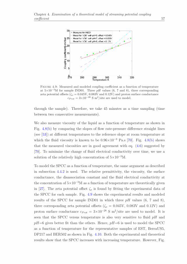
Chapter 4. Examination of a theoretical model of streaming potential couplingcoefficient 57
Figure 4.9: Measured and modeled coupling coefficient as a function of temperatureat 5×10⁻³M for sample IND01. Three pH values (6, 7 and 8), three correspondingzeta potential offsets (ζo = 0.045V, 0.083V and 0.12V) and proton surface conductance
cProt = 3×10⁻²⁸ S m2/site are used to model.
through the sample). Therefore, we take 45 minutes as a time sampling (time
between two consecutive measurements).
We also measure viscosity of the liquid as a function of temperature as shown in
Fig. 4.8(b) by comparing the slopes of flow rate-pressure difference straight lines
(see [53]) at different temperatures to the reference slope at room temperature at
which the fluid viscosity is known to be 0.96×10⁻³ Pa.s [70]. Fig. 4.8(b) shows
that the measured viscosities are in good agreement with eq. (4.6) suggested by
[70]. To minimize the change of fluid electrical conductivity over time, we use a
solution of the relatively high concentration of 5×10⁻³M.
To model the SPCC as a function of temperature, the same argument as described
in subsection 4.4.2 is used. The relative permittivity, the viscosity, the surface
conductance, the disassociation constant and the fluid electrical conductivity at
the concentration of 5×10⁻³M as a function of temperature are theoretically given
in [27]. The zeta potential offset ζo is found by fitting the experimental data of
the SPCC for each sample. Fig. 4.9 shows the experimental results and modeled
results of the SPCC for sample IND01 in which three pH values (6, 7 and 8),
three corresponding zeta potential offsets (ζo = 0.045V, 0.083V and 0.12V) and
proton surface conductance cProt = 3×10⁻²⁸ S m2/site are used to model. It is
seen that the SPCC versus temperature is also very sensitive to fluid pH and
pH=6 gives better fit than the others. Hence, pH=6 is used to model the SPCC
as a function of temperature for the representative samples of EST, BereaUS5,
DP217 and BER502 as shown in Fig. 4.10. Both the experimental and theoretical
results show that the SPCC increases with increasing temperature. However, Fig.

Chapter 4. Examination of a theoretical model of streaming potential couplingcoefficient 58
(a) (b)
(c) (d) Third caption
Figure 4.10: (a) is for the EST sample, (b) is for the BereaUS5 sample, (c) is for theDP217 sample and (d) is for the BER502 sample.
4.10 shows a essential deviation between the experimental data and the model.
The origin of that deviation is still unclear. One of the reasons may be due to a
temperature activated transport process happening around 300 K, which obviously
can not be explained by the model and requires further exploration.
4.5 Conclusion
We have measured the SPCC for 20 consolidated samples with 7 different concen-
tration NaCl solutions and 9 different temperatures under well controlled condi-
tions (pH, temperature, quality of distilled water). Afterwards the model is used
by taking fluid parameters, rock-fluid interface parameters already provided in [27]
and rock microstructure parameters (porosity, permeability and formation factor)
measured by ourself for all samples. The comparisons are carried out for each
sample.
Chapter 4. Examination of a theoretical model of streaming potential couplingcoefficient 59
For the concentration dependence of the SPCC, the comparison shows that the
theoretical model is not in agreement with the experimental data, especially in low
concentration range. However, if the zeta potential is considered to be constant
over a small range of electrolyte concentration the model fits the experimental data
very well. It leads to the suggestion that the formula of the zeta potential against
electrolyte concentration in the model needs to be recalculated and adjusted ac-
cordingly. In addition to the model given in [27], we also use other models to
predict the streaming potential as a function of electrolyte concentration. But all
applied models fail to fit the experimental data at low electrolyte concentration.
Therefore, further revisions of those models need to be carried out for a better fit
at low electrolyte concentration. Of all the models used for the comparison, the
modified model of Glover et al. [27] with assuming of constant zeta potential that
is experimentally measured is the best approach to predict the SPCC as a function
of electrolyte concentration. The modified model will in particular be useful in
situations where experiments are difficult to perform for a big range of electrolyte
concentration.
For temperature dependence of the SPCC, we implement a zeta potential offset
to the model which improve the fit to experimental data. The comparison shows
that the theoretical model does not fit well experimental data but it can repro-
duce the main trend of the experimental data. The reason for that could be due
to the variation of the input parameters over temperature because the streaming
potential coupling coefficient is sensitive to changes of the input parameters that
describe the rock/fluid interface, such as the surface site density (Γs), the binding
constant (KMe) and the disassociation constant (K(−)) [27]. Therefore, more re-
search about the change of the input parameters versus temperature needs to be
be carried out for a better explanation. A possible explanation of the deviation
at around 300K could be a temperature activated transport process. The results
also show that the model is very sensitive to the pH of the fluid, especially for the
streaming potential coupling coefficient as a function of temperature. So the fluid
pH needs to be carefully taken into account during measurements.

Chapter 5
Zeta potential of porous rocks in
contact with monovalent and
divalent electrolyte aqueous
solutions
5.1 Introduction
In chapter 2, chapter 3 and chapter 4, all streaming potential measurements of
porous media are carried out for NaCl solution only. However, in reality most
reservoir rocks are saturated or partially saturated by natural waters. Natural
waters normally contain mineral substances in the dissolved state (in the form of
ions, complex ions). The main cations contained in natural waters are Ca2+, Na+,
Mg2+ and K+ (mostly monovalent and divalent cations) and the main anions are
Cl−, SO42−, HCO3
− and CO32− [43]. Therefore, the study of how the streaming
potential coupling coefficient (SPCC) changes for different types of electrolytes is
very important in geophysical applications.
In electrolytes, cations normally called counterions for the systems of reservoir
rocks and electrolyte aqueous solutions influence the zeta potential most by affect-
ing the surface charge, by changing the thickness of the electric double layer and the
exact location of the shear plane [78]. The effect of counterions on the zeta poten-
tial on glass microchannels has been studied with Li+/Na+/K+/Ca2+/Ba2+[79],
Al3+/Na+[80], K+/Mg2+[81], Ca2+/Mg2+[82] and La3+/Na+[83]. Those studies
show that properties of counterions like ionic strength, ionic valence, ionic size
61
Chapter 5. Zeta potential of porous rocks in contact with monovalent and divalentelectrolyte aqueous solutions 62
and type of ions (monovalent, divalent or trivalent ions) affect the zeta potential.
The study of the zeta potential as a function of the electrolyte resistivity, pH,
and ionic compositions has also been carried out by Lorne et al. [84] for crushed
rocks. In this chapter, we study the dependence of types of electrolytes on the zeta
potential systematically for real porous reservoir rocks which are more relevant in
geophysical applications.
To do so, streaming potential measurements are carried out for 5 representative
consolidated samples (Bentheim Sandstone, Berea sandstone, Estaillade limestone,
Indiana Limestone and Artificial ceramic core) that are also used in chapter 4
with 11 different monovalent and divalent electrolyte aqueous solutions at the
concentration of 10−3 M. The electrolyte solutions used for the measurements are
NaI, NaCl, Na2SO4, KI, KCl, KNO3, CsCl, MgSO4, MgCl2, CaCl2 and CaSO4.
The reason for using the concentration of 10−3 M for all electrolytes is because
that concentration is a typical value normally found in water that is in contact
with the hydrocarbon-bearing formation [85]. From the SPCC with knowledge of
the electrical conductivity, viscosity and electrical permittivity of the fluid, the
zeta potential is obtained. Afterwards, the experimental results are analyzed in
combination with theoretical models.
For 1:1 electrolytes, a theoretical formula for the zeta potential that has been
already described in chapter 4 is used. For 2:2 electrolytes, we develop a new
model based on the same procedures mentioned in [25–27] for divalent electrolytes.
It should be noted that the models may not predict exactly absolute values of the
zeta potentials especially at low electrolyte concentration as shown in chapter 4
but they can explain quantitatively the change of the zeta potential against types
of electrolytes and types of rock. For a given electrolyte, the difference in the zeta
potential can be explained by the difference in the surface site density and the
disassociation constant for different kinds of porous rocks (mineral compositions).
For a given porous sample, the difference in the zeta potential can be explained by
the difference in the binding constant of cations and in cation types of electrolytes
(monovalent or divalent cations).
This chapter has four remaining sections. In the first we briefly describe theo-
retical models to calculate the zeta potential for both monovalent and divalent
electrolytes. In the second we present the experimental measurements. The third
section contains the experimental results, the comparison between the experimen-
tal and the theoretical results and the discussion. Conclusions are provided in the
final section.

Chapter 5. Zeta potential of porous rocks in contact with monovalent and divalentelectrolyte aqueous solutions 63
5.2 Theoretical background of the zeta potential
To calculate the zeta potential, one needs to know the Debye length (χd) and the
Stern potential (ϕd) as mentioned in chapter 4 (ζ =ϕdexp(−χζ/χd)). It should be
noted that the shear plane distance (χζ) is assumed to be constant for different
types of electrolytes [27].
For 1:1 electrolytes, NaCl for example, the denominator of the formula of the
Debye length mentioned in eq. (1.7) can be written as
∑ρ∞ie
2z2i = [Na+]e212 + [Cl−]e212 = 2[Na+]e2, ([Na+] = [Cl−])
= 2000CfNe2, ([Na+] is in ions/m3)(5.1)
where e is the elementary charge, N is the Avogadro’s number, [Na+] and [Cl−]
is the ionic concentrations of Na+ and Cl− in the bulk, respectively and Cf is
electrolyte concentration in mol/L.
Similarly, we obtain the expression of∑
ρ∞ie2z2i for 1:2 and 2:1 electrolytes and
2:2 electrolytes. Putting∑
ρ∞ie2z2i into eq. (1.7), the Debye length is expanded
for different types of electrolytes as below
χd =
⎧⎪⎪⎪⎪⎪⎪⎪⎨⎪⎪⎪⎪⎪⎪⎪⎩
√ε0εrkbT
2000Ne2Cf, For 1:1 electrolytes such as NaCl, KCl, NaI, KI, KNO3 and CsCl
√ε0εrkbT
6000Ne2Cf, For 1:2 and 2:1 electrolytes such as Na2SO4, MgCl2 and CaCl2√
ε0εrkbT8000Ne2Cf
, For 2:2 electrolytes such as CaSO4 and MgSO4
(5.2)
The Stern potential for different types of electrolytes is calculated as follows:
5.2.1 For 1:1 electrolytes
For 1:1 electrolytes, the Stern potential, ϕd, has an analytical form (see chapter 4
for more details):
ϕd =2kbT
3eln
(√8× 10³ε0εrkbTN(10−pH +KMeCf )
2eΓsK(−)
[Cf + 10−pH + 10pH−pKw√
Cf
]),
(5.3)
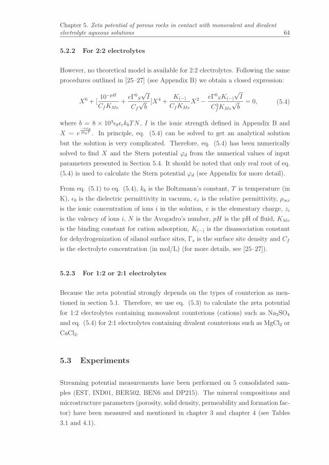
Chapter 5. Zeta potential of porous rocks in contact with monovalent and divalentelectrolyte aqueous solutions 64
5.2.2 For 2:2 electrolytes
However, no theoretical model is available for 2:2 electrolytes. Following the same
procedures outlined in [25–27] (see Appendix B) we obtain a closed expression:
X6 + [10−pH
CfKMe
+eΓ0
S
√I
Cf
√b]X4 +
K(−)CfKMe
X2 − eΓ0SK(−)
√I
C2fKMe
√b
= 0, (5.4)
where b = 8 × 10³ε0εrkbTN , I is the ionic strength defined in Appendix B and
X = e−eϕd2kbT . In principle, eq. (5.4) can be solved to get an analytical solution
but the solution is very complicated. Therefore, eq. (5.4) has been numerically
solved to find X and the Stern potential ϕd from the numerical values of input
parameters presented in Section 5.4. It should be noted that only real root of eq.
(5.4) is used to calculate the Stern potential ϕd (see Appendix for more detail).
From eq. (5.1) to eq. (5.4), kb is the Boltzmann’s constant, T is temperature (in
K), ε0 is the dielectric permittivity in vacuum, εr is the relative permittivity, ρ∞i
is the ionic concentration of ions i in the solution, e is the elementary charge, zi
is the valency of ions i, N is the Avogadro’s number, pH is the pH of fluid, KMe
is the binding constant for cation adsorption, K(−) is the disassociation constant
for dehydrogenization of silanol surface sites, Γs is the surface site density and Cf
is the electrolyte concentration (in mol/L) (for more details, see [25–27]).
5.2.3 For 1:2 or 2:1 electrolytes
Because the zeta potential strongly depends on the types of counterion as men-
tioned in section 5.1. Therefore, we use eq. (5.3) to calculate the zeta potential
for 1:2 electrolytes containing monovalent counterions (cations) such as Na2SO4
and eq. (5.4) for 2:1 electrolytes containing divalent counterions such as MgCl2 or
CaCl2.
5.3 Experiments
Streaming potential measurements have been performed on 5 consolidated sam-
ples (EST, IND01, BER502, BEN6 and DP215). The mineral compositions and
microstructure parameters (porosity, solid density, permeability and formation fac-
tor) have been measured and mentioned in chapter 3 and chapter 4 (see Tables
3.1 and 4.1).

Chapter 5. Zeta potential of porous rocks in contact with monovalent and divalentelectrolyte aqueous solutions 65
The experimental setup for the streaming potential measurement (at room tem-
perature - 22◦C) is shown in Fig. 3.1. The solutions used in the measurements
are 11 monovalent and divalent electrolyte aqueous solutions (NaCl, KCl, NaI,
Na2SO4, KNO3, CaSO4, CsCl, MgCl2, MgSO4, CaCl2 and KI) at the concentra-
tion of 10−3 M. All procedures of the measurement are the same as mentioned in
previous chapters.
5.4 Results and discussion
5.4.1 Streaming potential coupling coefficient versus electrolyte types
and and sample types
The way used to obtain the SPCC is the same as described in chapter 3 and chap-
ter 4. The SPCC for different electrolytes and different rocks is shown in Table
5.1. Based on Table 5.1, the dependence of the SPCC on types of electrolyte
for different samples is shown in Fig. 5.1. It shows that at a given sample, the
absolute values of the SPCC (|CS|) for monovalent electrolytes are higher than
that for divalent electrolytes. At a given electrolyte, |CS| is the highest for the
sample BEN6 (mostly silica) and the smallest for the sample IND (mostly calcite).
In other words, |CS| of the sample BEN6 saturated by monovalent electrolytes is
around 35 times as high as that of the sample IND saturated by divalent elec-
trolytes. This means that the coupling between the fluid flow and the electric
potential strongly depends on the mineral compositions of the rocks and types of
electrolytes. Because the coupling coefficient of the conversion between seismic
waves and electromagnetic waves is theoretically the product of a complicated ex-
pression of frequency and the SPCC [32], the system of Bentheim sandstone and
NaCl or NaI is one of the best ones for experimentally studying seismoelectric
effects.
5.4.2 Zeta potential versus electrolyte types and sample types
Viscosity, relative permittivity of electrolyte aqueous solutions and the formation
factor of the samples are already known (see Tables 3.1 and 4.1). The electrical
conductivity of the fully saturated samples are deduced from the sample resistances
measured by an impedance analyzer (Hioki IM3570) [65]. Therefore, the zeta
potential for different electrolytes is obtained based on eq. 1.9 as reported in
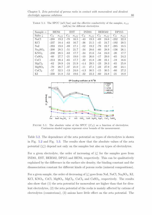
Chapter 5. Zeta potential of porous rocks in contact with monovalent and divalentelectrolyte aqueous solutions 66
Table 5.1: The SPCC (mV/bar) and the effective conductivity of the samples, σeff
(mS/m) for different electrolytes
Sample→ BEN6 EST IND01 BER502 DP215
Salts ↓ CS σeff CS σeff CS σeff CS σeff CS σeffNaCl -288 19.2 -78 16.5 -43 19.3 -69 24.6 -232 22.3KCl -237 18.4 -63 16.7 -36 21.5 -45 24.7 -192 20.5NaI -293 19.8 -89 17.1 -52 19.2 -79 23.7 -285 18.5Na2SO4 -200 28.5 -51 21.7 -34 28.6 -60 28.9 -136 26.1KNO3 -230 20.5 -63 17.7 -34 21.6 -54 24.0 -20 17.7CaSO4 -60 27.7 -21 19.0 -10 26.0 -17 29.0 -65 24.2CsCl -213 20.4 -65 17.7 -32 21.8 -39 23.1 -19 16.6MgCl2 -62 28.9 -24 21.9 -4.4 29.5 -23 28.3 -65 25.8MgSO4 -70 28.7 -37 21.0 -11 27.1 -23 27.9 -80 24.1CaCl2 -57 32.5 -13 24.0 -4.3 30.5 -15 30.5 -60 27.2KI -230 21.8 -52 19.6 -32 22.3 -60 24.8 -21 18.8
Figure 5.1: The absolute value of the SPCC (|CS |) as a function of electrolytes.Continuous shaded regions represent error bounds of the measurement.
Table 5.2. The dependence of the zeta potential on types of electrolytes is shown
in Fig. 5.2 and Fig. 5.3. The results show that the absolute values of the zeta
potential (|ζ|) depend not only on the samples but also on types of electrolytes.
For a given electrolyte, the order of increasing of |ζ| for the samples goes from
IND01, EST, BER502, DP215 and BEN6, respectively. This can be qualitatively
explained by the difference in the surface site density, the binding constant and the
disassociation constant for different kinds of porous rocks (mineral compositions).
For a given sample, the order of decreasing of |ζ| goes from NaI, NaCl, Na2SO4, KI,
KCl, KNO3, CsCl, MgSO4, MgCl2, CaCl2 and CaSO4, respectively. The results
also show that (1) the zeta potential for monovalent are higher than that for diva-
lent electrolytes, (2) the zeta potential of the rocks is mainly affected by cations of
electrolytes (counterions), (3) anions have little effect on the zeta potential. The

Chapter 5. Zeta potential of porous rocks in contact with monovalent and divalentelectrolyte aqueous solutions 67
Table 5.2: Zeta potential (mV)
�����������SaltsSample
BEN6 EST IND01 BER502 DP215
NaCl -78.1 -18.1 -11.6 -23.9 -73.2KCl -65.9 -14.8 -10.9 -15.6 -55.5NaI -84.3 -21.5 -14.1 -26.5 -74.5
Na2SO4 -80.5 -15.6 -13.6 -24.4 -50.1KNO3 -66.7 -15.6 -10.5 -18.2 -50.8CaSO4 -23.3 -5.7 -4.0 -6.8 -22.6CsCl -61.4 -16.1 -9.7 -12.6 -44.5MgCl2 -25.8 -7.3 -1.8 -9.3 -23.3MgSO4 -28.2 -11.0 -4.2 -9.1 -27.2CaCl2 -26.3 -4.3 -1.9 -6.6 -23.0KI -70.7 -14.3 -10.2 -21.0 -56.7
Figure 5.2: The absolute value of the zeta potential as a function of electrolytes.Continuous shaded regions represent error bounds of the measurement.
Figure 5.3: The absolute value of the zeta potential as a function of electrolytes

Chapter 5. Zeta potential of porous rocks in contact with monovalent and divalentelectrolyte aqueous solutions 68
difference in the zeta potential for a given sample can be qualitatively explained
by the difference in the binding constant of cations and in types of cations (mono-
valent or divalent cations). For example, for the same type of cations (monovalent
cations), the binding constant of K+ is larger than Na+ [27]. Therefore, at the
same concentration more cations of K+ are absorbed on the negative solid surface
than cations of Na+. This makes the electric potential on the shear plane (the
zeta potential) smaller in the electrolyte containing K+ that that in the electrolyte
containing Na+.
To quantitatively explain the behaviors in Fig. 5.2 and Fig. 5.3, we use the
theoretical formulas mentioned in Section 5.2 to calculate the zeta potential us-
ing the input parameters that are already available in literature. For the sample
BEN6, the mineral composition is mainly silica (see Table 4.1). Thus, we use input
parameters given in the work of Glover at al. [27] for silica. The value of the dis-
association constant, K(−), for dehydrogenization of silanol surface sites is taken
as 10−7.1. The shear plane distance, χζ , is taken as 2.4×10⁻¹⁰m. The surface site
density, Γs, is taken as 5×10¹⁸ site/m2. The disassociation constant of water, Kw,
at 22◦C is 9.22×10⁻¹⁵. The fluid pH is 6.7. The binding constant for cation adsorp-
tion on silica varies according to which is the dominant cations in the electrolyte
and it is not well known. For example, KMe(Li+)=10−7.8 and KMe(Na
+)=10−7.1
for silica given by Dove Rimstidt [86], KMe(Li+)=10−7.7, KMe(Na
+)=10−7.5 and
KMe(Cs+)=10−7.2 given by Kosmulski and Dahlsten [87], KMe(Na
+)=10−3.25 and
KMe(K+)=10−2.8 given by Revil et al. [26]. By fitting experimental data for the
zeta potential as shown in Fig. 5.4 for the sample BEN6, the binding constants for
cations are obtained as KMe(Na+)=10−5.5, KMe(K
+)=10−3.3, KMe(Cs+)=10−2.9,
KMe(Mg2+)=10−5.2 and KMe(Ca2+)=10−5.0. The binding constants for Na+, K+
and Cs+ are in very good agreement with those given by Scales et al. [88]
(KMe(Na+)=10−5.5, KMe(K
+)=10−3.2, KMe(Cs+)=10−2.8). The binding constant
of Mg2+ is lower than that of Ca2+ due to the stronger absorption of Ca2+ as
shown in [82].
For the sample DP215, because its mineral composition (mostly alumina and fused
silica as shown in see Table 4.1) is not the same as that of the sample BEN6, the
rock/fluid interface parameters of the sample DP215 will be different from the
sample BEN6. However, based on the theoretical model mentioned in Section 5.2,
it is seen that the surface site density affects the zeta potential much more than
the disassociation constant and the binding constant. Therefore, we keep all input
parameters the same as above for the sample BEN6 except the surface site density.
By fitting the experimental data (see Fig. 5.5), the surface site density for sample

Chapter 5. Zeta potential of porous rocks in contact with monovalent and divalentelectrolyte aqueous solutions 69
Figure 5.4: The absolute value of the zeta potential as a function of electrolytes for thesample BEN6. Continuous shaded regions represent error bounds of the measurement.
Figure 5.5: The absolute value of the zeta potential as a function of electrolytes for thesample DP215. Continuous shaded regions represent error bounds of the measurement
DP215 is found to be Γs=2.5×10¹⁸ site/m2. That value is lower than that of the
sample BEN6.
For the samples BER502, EST and IND01, it is hard to quantitatively explain the
experimental data by the models. The reason is that the mineral composition of
those samples is a mixture of several minerals. Therefore, all input parameters such
as the surface site density, the disassociation constant and the binding constant or
the shear plane distance are not known well enough to be applied in the models.
It should be noted that the theoretical predictions do not show the effect of anions
on the zeta potential as shown Fig. 5.4 and Fig. 5.5 (for example, the zeta
potential is the same for NaCl and NaI). However, the experimental data shows
that anions have a little effect on the zeta potential. Criscenti and Sverjensky [89]
also show that electrolyte anions play a role in metal cation adsorption on the
solid surfaces in salt solutions. Therefore, they influence the zeta potential. It
suggests that the models need to be improved to take into account the effect of
electrolyte anions.

Chapter 5. Zeta potential of porous rocks in contact with monovalent and divalentelectrolyte aqueous solutions 70
Figure 5.6: Zeta potential as a function of electrolyte concentration for 1:1 electrolytesand 2:2 electrolytes
To predict how the zeta potential behaves against the electrolyte concentration
and the fluid pH for 2:2 electrolytes, we solve eq. (5.4) numerically to find X.
The silica based sample and the 2:2 electrolyte of MgSO4, for example, are used
for the prediction. Therefore, input parameters for eq. (5.4) are K(−)= 10−7.1,
χζ=2.4×10⁻¹⁰m, Γs=5×10¹⁸ site/m2, andKMe=10−5.2 (for the adsorption of coun-
terion Mg2+ on the silica surface). From the solution X, the Stern potential ϕd
and therefore the zeta potential have been obtained as a function of electrolyte
concentration (the solid line in Fig. 5.6) and pH (the solid line in Fig. 5.7).
Based on Eq. (4.4), Eq. (5.2) and Eq. (5.3), we also predict the change of the zeta
potential against the electrolyte concentration and the fluid pH for 1:1 electrolytes.
The same argument for 2:2 electrolytes is used for the silica based sample and the
1:1 electrolyte of KCl. Therefore, the same input parameters as above (K(−), χζ ,
Γs) are used except KMe=10−3.3 (for the adsorption of counterion K+ on the silica
surface). The change of the zeta potential against electrolyte concentration and
fluid pH for 1:1 electrolytes are shown in Fig. 5.6 (the dashed line) and Fig. 5.7
(the dashed line), respectively.
Fig. 5.6 and Fig. 5.7 show that the zeta potential as a function of electrolyte
concentration and pH have the same behaviors for both 1:1 and 2:2 electrolytes.
The zeta potential in magnitude decreases with increasing electrolyte concentra-
tion and with decreasing fluid pH for both types of electrolytes. The theoretical
values of the zeta potential for 2:2 electrolytes are less dependent on the fluid pH
than those for 1:1 electrolytes. The reason is that the absorption process of the
divalent cations is much less sensitive to pH as stated in [82].
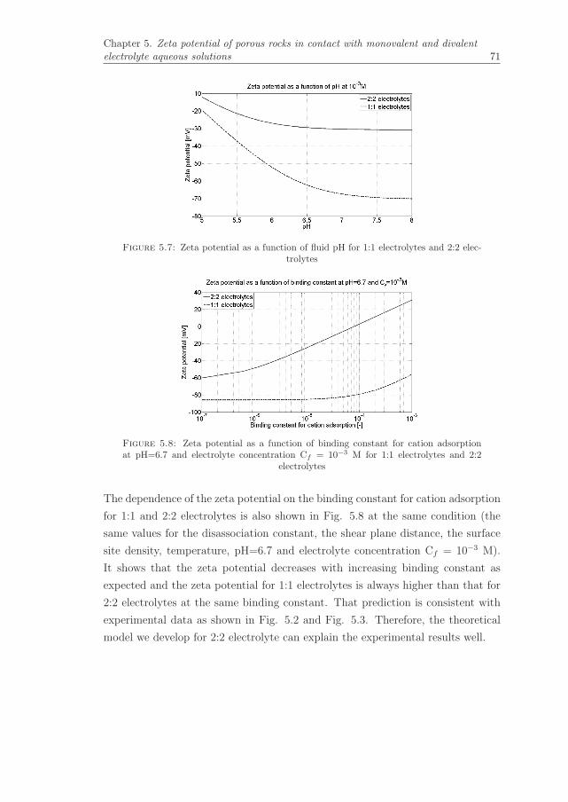
Chapter 5. Zeta potential of porous rocks in contact with monovalent and divalentelectrolyte aqueous solutions 71
Figure 5.7: Zeta potential as a function of fluid pH for 1:1 electrolytes and 2:2 elec-trolytes
Figure 5.8: Zeta potential as a function of binding constant for cation adsorptionat pH=6.7 and electrolyte concentration Cf = 10−3 M for 1:1 electrolytes and 2:2
electrolytes
The dependence of the zeta potential on the binding constant for cation adsorption
for 1:1 and 2:2 electrolytes is also shown in Fig. 5.8 at the same condition (the
same values for the disassociation constant, the shear plane distance, the surface
site density, temperature, pH=6.7 and electrolyte concentration Cf = 10−3 M).
It shows that the zeta potential decreases with increasing binding constant as
expected and the zeta potential for 1:1 electrolytes is always higher than that for
2:2 electrolytes at the same binding constant. That prediction is consistent with
experimental data as shown in Fig. 5.2 and Fig. 5.3. Therefore, the theoretical
model we develop for 2:2 electrolyte can explain the experimental results well.
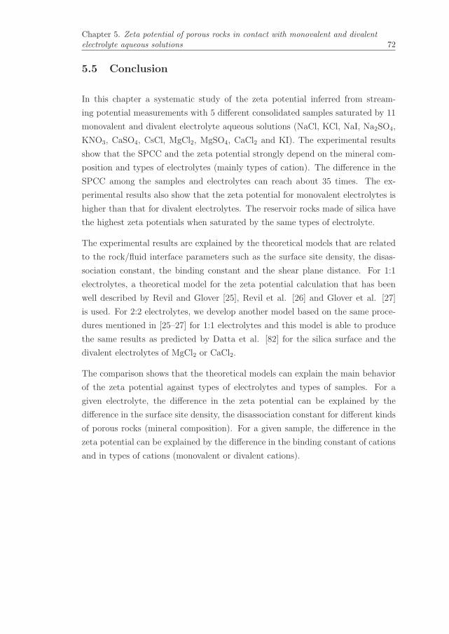
Chapter 5. Zeta potential of porous rocks in contact with monovalent and divalentelectrolyte aqueous solutions 72
5.5 Conclusion
In this chapter a systematic study of the zeta potential inferred from stream-
ing potential measurements with 5 different consolidated samples saturated by 11
monovalent and divalent electrolyte aqueous solutions (NaCl, KCl, NaI, Na2SO4,
KNO3, CaSO4, CsCl, MgCl2, MgSO4, CaCl2 and KI). The experimental results
show that the SPCC and the zeta potential strongly depend on the mineral com-
position and types of electrolytes (mainly types of cation). The difference in the
SPCC among the samples and electrolytes can reach about 35 times. The ex-
perimental results also show that the zeta potential for monovalent electrolytes is
higher than that for divalent electrolytes. The reservoir rocks made of silica have
the highest zeta potentials when saturated by the same types of electrolyte.
The experimental results are explained by the theoretical models that are related
to the rock/fluid interface parameters such as the surface site density, the disas-
sociation constant, the binding constant and the shear plane distance. For 1:1
electrolytes, a theoretical model for the zeta potential calculation that has been
well described by Revil and Glover [25], Revil et al. [26] and Glover et al. [27]
is used. For 2:2 electrolytes, we develop another model based on the same proce-
dures mentioned in [25–27] for 1:1 electrolytes and this model is able to produce
the same results as predicted by Datta et al. [82] for the silica surface and the
divalent electrolytes of MgCl2 or CaCl2.
The comparison shows that the theoretical models can explain the main behavior
of the zeta potential against types of electrolytes and types of samples. For a
given electrolyte, the difference in the zeta potential can be explained by the
difference in the surface site density, the disassociation constant for different kinds
of porous rocks (mineral composition). For a given sample, the difference in the
zeta potential can be explained by the difference in the binding constant of cations
and in types of cations (monovalent or divalent cations).

Chapter 6
Streaming potential
measurements on the binary
mixture Triethylamine - water
near the demixing phase
transition
6.1 Introduction
In previous chapters, electrolyte aqueous solutions have been used for the stream-
ing potential and electroosmosis measurements. However, in reality the liquids
found underground can be a complicated mixture of water, crude oil and gas. It
should be noted that at a certain condition (high temperature and high pressure),
oil and water can mix together [90]. Therefore, it is worthwhile studying elec-
trokinetic phenomena in liquid mixtures. The effect of the compositions on the
electrokinetic phenomena happening in some liquid mixtures have been reported in
the literature. For example, the influences of the compositions on the electrophore-
sis [91, 92], on the electroosmosis [93, 94], and on the streaming potential [93] have
been carried out with liquid mixtures such as methanol-water, ethanol-water,
2-propanol-water, 1-propanol-water, methanol-acetone-water, alcohol-water and
acetone-water. The results of those studies have shown that the compositions
of the mixtures affect the electrokinetic coupling coefficient. The changes of the
electrokinetic coupling coefficient have been explained by both the change of the
73
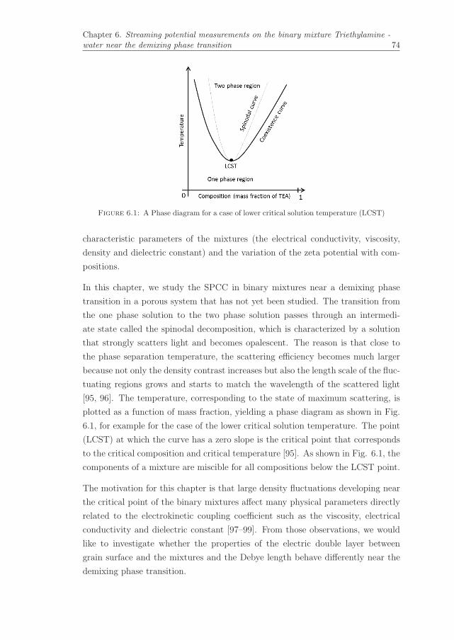
Chapter 6. Streaming potential measurements on the binary mixture Triethylamine -water near the demixing phase transition 74
Figure 6.1: A Phase diagram for a case of lower critical solution temperature (LCST)
characteristic parameters of the mixtures (the electrical conductivity, viscosity,
density and dielectric constant) and the variation of the zeta potential with com-
positions.
In this chapter, we study the SPCC in binary mixtures near a demixing phase
transition in a porous system that has not yet been studied. The transition from
the one phase solution to the two phase solution passes through an intermedi-
ate state called the spinodal decomposition, which is characterized by a solution
that strongly scatters light and becomes opalescent. The reason is that close to
the phase separation temperature, the scattering efficiency becomes much larger
because not only the density contrast increases but also the length scale of the fluc-
tuating regions grows and starts to match the wavelength of the scattered light
[95, 96]. The temperature, corresponding to the state of maximum scattering, is
plotted as a function of mass fraction, yielding a phase diagram as shown in Fig.
6.1, for example for the case of the lower critical solution temperature. The point
(LCST) at which the curve has a zero slope is the critical point that corresponds
to the critical composition and critical temperature [95]. As shown in Fig. 6.1, the
components of a mixture are miscible for all compositions below the LCST point.
The motivation for this chapter is that large density fluctuations developing near
the critical point of the binary mixtures affect many physical parameters directly
related to the electrokinetic coupling coefficient such as the viscosity, electrical
conductivity and dielectric constant [97–99]. From those observations, we would
like to investigate whether the properties of the electric double layer between
grain surface and the mixtures and the Debye length behave differently near the
demixing phase transition.

Chapter 6. Streaming potential measurements on the binary mixture Triethylamine -water near the demixing phase transition 75
Figure 6.2: The core holder
We perform the streaming potential measurements with the Triethylamine-water
binary mixture (TEA-W) using an artificial ceramic porous sample. This mixture
is a typical partially miscible system that has a lower critical solution temperature
near room temperature at atmospheric pressure. The critical composition and
critical temperature of the mixture are Cc = 32.1 % of TEA mass fraction and
18.24oC < Tc < 18.40oC, respectively [97, 99]. Three different mass fractions
of TEA (20%, 32.1% and 70%) are used for the measurements. Based on the
measured streaming potential coupling coefficient (SPCC) with the knowledge of
the electrical conductivity, viscosity and dielectric constant, the zeta potentials
are obtained.
This chapter includes four sections. Section 6.2 presents the experimental setup,
materials and procedures for collecting experimental data. Section 6.3 contains
the experimental results and discussion. Conclusions are provided in Section 6.4.
6.2 Experiments
6.2.1 Setup
The experimental setup for the measurement of the streaming potential is similar
as described in chapter 4 for measuring the SPCC as a function of temperature.
To control temperature of the mixture, the core holder (see Fig. 6.2) and the

Chapter 6. Streaming potential measurements on the binary mixture Triethylamine -water near the demixing phase transition 76
solution container in which a mixture of TEA and water has been mixed together
is immersed in a thermally stabilized water bath (Thermo Fisher Scientific SC150
and A25). The sample in the core holder is surrounded by a conical teflon sleeve
inserted into a teflon cell as shown in Fig. 6.2. By tightly twisting the caps, the
fluid can be prevented to flow along the interface of the sample. Rubber seals are
not used in the setup because TEA dissolves rubber.
The pressure differences across the sample are created by the high pressure pump
(LabHut Series III- Pump) and measured by the pressure transducer (Endress and
Hauser Deltabar S PMD75). The electrical potential difference across the sample
is measured by two Ag/AgCl wire electrodes. The Ag/AgCl electrodes are made
by electrolysis of a wire of clean silver from VWR company in 0.1M NaCl with an
electrical current of 20 mA and in 2 minutes [3]. The electrodes are covered by
heat shrinkable teflon tubings and their tips are put in the vicinity of each face of
the sample but not within the liquid circulation to avoid the electrical noise from
liquid movement around the electrodes [36]. The way used to obtain the SPCC as
a function of temperature is described in chapter 4.
6.2.2 Materials
The triethylamine (TEA) is purchased from VWR (Merck). The purity is stated to
be 99.95 %. The TEA is used without further purification. The water used in this
work is deionized water. All mixtures are prepared from weighed amounts of the
pure components. Besides the critical composition (32.1% mass fraction of TEA),
two other mass fractions (20% and 70%) are also used for the measurements. It
should be noted that the mixture of TEA and water used in this chapter may be
not really clean because of mineral substances of the sample that may dissolve
in the mixture or impurities (e.g., CO2, H2O) of the mixtures. Therefore, 32.1%
mass fraction of TEA may not exactly be the critical composition as stated in
literature, for example in [97–99].
The porous sample is a cylindrical artificial core made of alumina (72%) and fused
silica (28%) from HP Technical Ceramics (55 mm in length and 25mm in diameter).
The properties of the sample have been reported in Table 3.1 for the one labeled
DP217: the permeability of 370 mD, the porosity of 45.4%, the solid density of
3652 kg/m3 and the formation factor of 4.5.

Chapter 6. Streaming potential measurements on the binary mixture Triethylamine -water near the demixing phase transition 77
Figure 6.3: Streaming potential coupling coefficient as a function of temperature at 3different mass fractions of TEA (20%, 32.1% and 70% mass). The disconnected points
are the measured data points. The solid lines are the fitted lines
6.3 Results and discussion
The experimental measurements are carried out in the single phase in the neigh-
borhood of the demixing phase transition temperature and relatively far from this
temperature. The transition temperature for the 32.1% composition is visually
identified to be 20.2◦ C in our laboratory when the opalescence is well developed
in the glass container that can be seen through. If the mixture is cooled down to
10◦ C and stirred, a single phase solution is formed in the container. The con-
tainer is then slowly heated up until the entire volume of the solutions becomes
white and the opalescence is easily visible due to strong light scattering. The
critical temperature is shifted to a higher value compared to the known critical
temperature Tc = 18.4o C [97] or 18.242oC < Tc < 18.253oC [99]. The reason
for this discrepancy is likely due to impurities (e.g., CO2, H2O) of the mixtures
and the ability of the strongly basic triethylamine to attack glass [95]. Using the
same procedure to obtain the demixing temperatures (Tdemix) for two other mass
fractions, we get the Tdemix of 21◦ C and 19◦ C for the mass fractions of 20% and
70%, respectively.
To see how the SPCC and the zeta potential behave around the phase transition
point, temperature is scanned from 10◦ C to Tdemix (21◦ C, 20.2◦ and 19◦ C for
the mass fractions of 20%, 32.1% and 70%, respectively). If temperature was
raised higher than the Tdemix, the solution pumped through the sample would be
either TEA or water rather than the mixture due to the phase separation. The
separation between mixed and demixed mixtures is roughly indicated by the faint
lines as shown in Fig. 6.3 and Fig. 6.4.

Chapter 6. Streaming potential measurements on the binary mixture Triethylamine -water near the demixing phase transition 78
Figure 6.4: Electrical conductivity of the mixtures as a function of temperature at3 different mass fraction of TEA (20%, 32.1% and 70%). The disconnected points are
the measured data points and the solid lines are the fitted lines
The SPCC as a function of temperature in one phase solution at 3 different mass
fractions of TEA is shown in Fig. 6.3 by the points. It is seen that the SPCC in
magnitude decreases with increasing temperature. This observation is opposite to
what has been observed in our earlier work (see chapter 4) for the same sample
(DP217) but with the NaCl solution in which the SPCC increases with increasing
temperature. It suggests that there is a difference in the properties of the EDL
between using the TEA-W mixture and using the NaCl solution. Fig. 6.3 also
shows that there seems to be no an anomaly of the SPCC when temperature
approaches the Tdemix.
In order to calculate the zeta potential from the measured SPCC, one needs to
know the electrical conductivity, viscosity and dielectric constant of the mixtures.
The electrical conductivity of the mixtures as a function of temperature is directly
measured by the conductivity meter (Consort C861) and is shown in Fig. 6.4 by
the points. It shows that the electrical conductivity of the binary mixture increases
with increasing temperature as expected in [100] in which the relationship between
the electrical conductivity and temperature is given by Vogel-Fulcher-Tammann
(VFT) equation
σ = A exp(− B
T − Tg
), (6.1)
where A, B and Tg are fitting parameters. By fitting the experimental data to
eq. (6.1), the values of the parameters A, B and Tg at 3 different mass fractions
of TEA (20%, 32.1% and 70%) are found to be 0.42 mS/cm, 78.0K−1, 238.0K;
0.37mS/cm, 102.0K−1, 241.0K and 0.04mS/cm, 68.0K−1, 249.5K, respectively.
According to [100], close to the demixing temperature the electrical conductivity
deviates slightly from the regular VFT behavior. This deviation becomes bigger

Chapter 6. Streaming potential measurements on the binary mixture Triethylamine -water near the demixing phase transition 79
Figure 6.5: Viscosity of the mixtures as a function of temperature at 3 differentmass fraction of TEA (20%, 32.1% and 70%). The experimental data is obtained from[97, 100] for clean mixtures. The dash lines are the ones connecting the experimental
points.
when the temperature of the mixture approaches the demixing temperature. How-
ever, the deviation of the electrical conductivity from the regular VFT behavior
is not really clear around the demixing point as observed in [100]. Therefore, we
use the VFT equation only to relate the electrical conductivity of binary fluid
mixtures to temperature in the single phase region (T ≤ Tdemix) as shown in Fig.
6.4 (the solid lines).
Temperature dependence of viscosity of the binary mixtures in the single phase
has been experimentally measured at 3 different mass fractions of TEA (20%,
32.1% and 70%) in the works of [97, 100] for the clean mixtures as shown in Fig.
6.5. It is shown that when the temperature approaches the critical temperature
(TC), the critical fluctuations cause a further increase of the viscosity for the
critical composition (32.1%). It is also seen that viscosity is maximum at a critical
composition (32.1%) of three mass fractions of TEA. That could be explained by
the model suggested by [101] in which the viscosity of the liquid mixtures at a
given temperature can be calculated by
ln η = w1 ln η1 + w2 ln η2 + w1w2G12, (6.2)
where w1, w2, η1 and η2 are mass fraction of TEA, mass fraction of water, viscosity
of TEA and viscosity of water, respectively. G12 is a parameter depending on
temperature. For example, G12 = 9.01 at 10◦C (see [101]. From eq. (6.2) the
variation of the viscosity versus TEA mass fraction for Triethylamine (1) + water
(2) mixture at 10◦C is shown in Fig. 6.6.
The dielectric constant as a function of temperature in the single phase region

Chapter 6. Streaming potential measurements on the binary mixture Triethylamine -water near the demixing phase transition 80
Figure 6.6: The variation of the viscosity versus TEA mass fraction for Triethylamine(1) + water (2) mixture at 10◦C, G12 = 9.01 (see [101]).
of the binary mixture for the critical composition has been reported by [99]. By
extrapolating the experimental data of [99], the temperature dependence of dielec-
tric constant of the mixture at the critical composition is shown in Fig. 6.7. The
result shows that the dielectric constant fluctuates near the critical point.
Since the dielectric constants of the binary mixtures at the other two mass fractions
(20% and 70%) are not yet available in literatures, we use a parallel plate copper
capacitor to measure them. When the plate capacitor is gradually immersed, the
capacitance changes in proportion to the depth by which the plates are immersed
into the dielectric liquid. Fig. 6.8 shows the capacitance against the depth for TEA
only and 70% mass fraction of TEA at 10◦C. From the slopes of the straight lines,
the dielectric constants of TEA only and 70% mass fraction of TEA are determined
to be 16.2 and 2.6, respectively. The dielectric constant of 2.6 for TEA only is
in good agreement with that mentioned in [54] (2.42). That shows the validity of
the dielectric constant measurement. For 20% mass fraction of TEA, the electrical
conductivity of the mixture is too high to measure the dielectric constant for our
setup. We approximately use the dielectric constant of water (80) for the mixture
of 20% mass fraction of TEA. According to [54], the dielectric constants of TEA
only and water change only 0.8% in the temperature range 10◦C to 21◦C. We
therefore assume that the dielectric constants are constant over temperature for
the purpose of calculating the zeta potential.
Because the binary mixtures that we use for the measurements may be different
from those used in the works of [97, 100] and [99] due to the impurities. This
is indicated by the shift of TC to higher temperatures at the nominal critical
composition of 32.1%. The variations of viscosity and dielectric constant of the
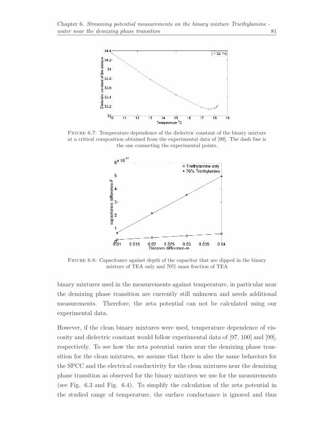
Chapter 6. Streaming potential measurements on the binary mixture Triethylamine -water near the demixing phase transition 81
Figure 6.7: Temperature dependence of the dielectric constant of the binary mixtureat a critical composition obtained from the experimental data of [99]. The dash line is
the one connecting the experimental points.
Figure 6.8: Capacitance against depth of the capacitor that are dipped in the binarymixture of TEA only and 70% mass fraction of TEA
binary mixtures used in the measurements against temperature, in particular near
the demixing phase transition are currently still unknown and needs additional
measurements. Therefore, the zeta potential can not be calculated using our
experimental data.
However, if the clean binary mixtures were used, temperature dependence of vis-
cosity and dielectric constant would follow experimental data of [97, 100] and [99],
respectively. To see how the zeta potential varies near the demixing phase tran-
sition for the clean mixtures, we assume that there is also the same behaviors for
the SPCC and the electrical conductivity for the clean mixtures near the demixing
phase transition as observed for the binary mixtures we use for the measurements
(see Fig. 6.3 and Fig. 6.4). To simplify the calculation of the zeta potential in
the studied range of temperature, the surface conductance is ignored and thus

Chapter 6. Streaming potential measurements on the binary mixture Triethylamine -water near the demixing phase transition 82
Figure 6.9: The prediction of the zeta potential as a function of temperature at threedifferent mass fractions of TEA for clean binary mixtures. The dash lines are the ones
connecting the experimental points.
the zeta potential is calculated using eq. (1.2). By fitting the experimental data
shown in Fig. 6.3 and Fig. 6.4 (see solid lines), the relationship between the
SPCC and the electrical conductivity against temperature at three different mass
fractions of clean mixtures are obtained. With the knowledge of viscosity and di-
electric constant obtained from [97, 100] and [99], the zeta potential as a function
of temperature at three different mass fractions is obtained and shown in Fig. 6.9.
The prediction shows that zeta potential at the critical composition (32.1%) for
clean mixture may behave differently around the critical point if the viscosity and
dielectric constant follow what has been measured in [97, 100] and [99]. However,
it seems that there is no an anomaly happening around the demixing point for
the other two mass fractions. Absolute values of the zeta potential decreases
with increasing temperature. That is opposite to what has been observed in our
earlier work (see chapter 4) in which the zeta potential increases with increasing
temperature for the NaCl solution. It means that the TEA-W binary mixtures
change the properties of the electric double layer and the zeta potential compared
to normal aqueous electrolytes. Fig. 6.9 also shows that the zeta potential varies
with compositions of the mixtures as observed [91–94] for liquid mixtures such
as methanol-water, ethanol-water, 2-propanol-water, 1-propanol-water, methanol-
acetone-water, alcohol-water and acetone-water.
6.4 Conclusions
The streaming potential measurements for the porous material saturated with a
binary mixture of triethylamine-water with three different mass fractions have
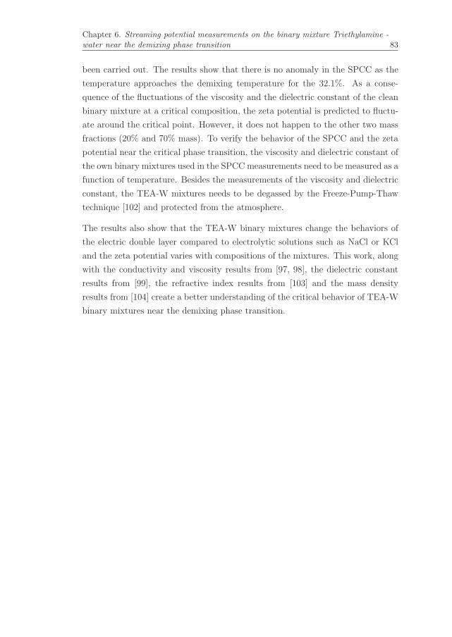
Chapter 6. Streaming potential measurements on the binary mixture Triethylamine -water near the demixing phase transition 83
been carried out. The results show that there is no anomaly in the SPCC as the
temperature approaches the demixing temperature for the 32.1%. As a conse-
quence of the fluctuations of the viscosity and the dielectric constant of the clean
binary mixture at a critical composition, the zeta potential is predicted to fluctu-
ate around the critical point. However, it does not happen to the other two mass
fractions (20% and 70% mass). To verify the behavior of the SPCC and the zeta
potential near the critical phase transition, the viscosity and dielectric constant of
the own binary mixtures used in the SPCC measurements need to be measured as a
function of temperature. Besides the measurements of the viscosity and dielectric
constant, the TEA-W mixtures needs to be degassed by the Freeze-Pump-Thaw
technique [102] and protected from the atmosphere.
The results also show that the TEA-W binary mixtures change the behaviors of
the electric double layer compared to electrolytic solutions such as NaCl or KCl
and the zeta potential varies with compositions of the mixtures. This work, along
with the conductivity and viscosity results from [97, 98], the dielectric constant
results from [99], the refractive index results from [103] and the mass density
results from [104] create a better understanding of the critical behavior of TEA-W
binary mixtures near the demixing phase transition.


Appendix A
Parameters of porous samples
In our study, we use two types of porous samples including unconsolidated samples
and consolidated samples. The parameters used to characterize porous media are
the porosity φ, density of grains ρs, tortuosity α∞, formation factor F and steady-
state permeability ko. All parameters are measured by independent laboratory
experiments for both types of porous samples. In addition, we also measure the
frame and the shear modulus of the consolidated samples (KP and GS). Here we
present the approaches and experimental setups to measure those parameters.
A.1 Porosity
The porosity is measured by a simple method [48]: The sample is first dried in
oven for 24 hours, cooled to room temperature and fully saturated with deionized
water under vacuum. The sample is weighed before (mdry) and after saturation
(mwet), and the porosity is determined as:
φ =(mwet −mdry)/ρ
AL, (A.1)
A.2 Solid density
The solid density ρs is determined from
ρs =mdry
(1− φ)AL, (A.2)
85

Appendix A. Parameters of porous samples 86
Figure A.1: Constant flow-rate setup for permeability measurement
where ρ is density of the deionized water, A and L are the cross sectional area and
the physical length of the samples, respectively.
A.3 Permeability
Steady-state permeability can be determined by a constant flow-rate experiment
as shown in Fig. A.1. A high pressure pump (LabHut, Series III- Pump) ensures a
constant flow through the sample, a high precision differential pressure transducer
(Endress and Hauser Deltabar S PMD75) is used to measure the pressure drop.
For low velocities, Darcy’s law holds
Qf = −k0A
η
ΔP
L, (A.3)
where Qf is the fluid volume flow rate, k0 is the permeability, ΔP is the differential
pressure imposed across the sample, η is the viscosity of the fluid. Fig. A.2 plots
the flow rate against pressure difference for repeated experiments on the sample
BereaUS5. The permeability is determined from the slope of the straight lines
shown in Fig. A.2. The final permeability is the mean value of two calculated
permeabilities. The linear trend verifies the applicability of Darcy’s law as ex-
pected from the maximum Reynolds number of 0.05 for our study. That value is
much smaller than the critical maximum value, Re = 1 below which fluid flows
are creeping flows (for more details, see [105]). The Reynolds number is defined
as [106]
Re =ρvl
η, (A.4)
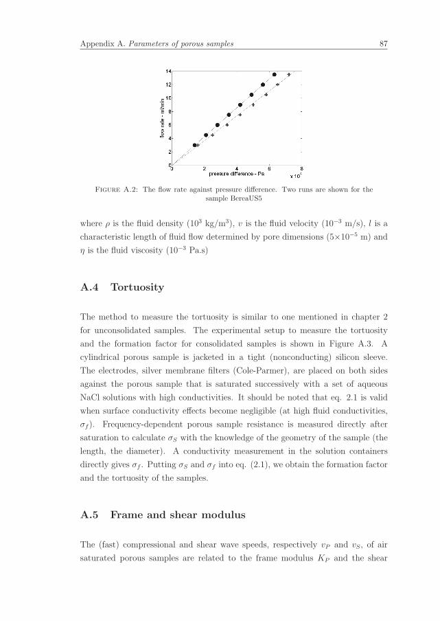
Appendix A. Parameters of porous samples 87
Figure A.2: The flow rate against pressure difference. Two runs are shown for thesample BereaUS5
where ρ is the fluid density (103 kg/m3), v is the fluid velocity (10−3 m/s), l is a
characteristic length of fluid flow determined by pore dimensions (5×10⁻⁵ m) and
η is the fluid viscosity (10−3 Pa.s)
A.4 Tortuosity
The method to measure the tortuosity is similar to one mentioned in chapter 2
for unconsolidated samples. The experimental setup to measure the tortuosity
and the formation factor for consolidated samples is shown in Figure A.3. A
cylindrical porous sample is jacketed in a tight (nonconducting) silicon sleeve.
The electrodes, silver membrane filters (Cole-Parmer), are placed on both sides
against the porous sample that is saturated successively with a set of aqueous
NaCl solutions with high conductivities. It should be noted that eq. 2.1 is valid
when surface conductivity effects become negligible (at high fluid conductivities,
σf ). Frequency-dependent porous sample resistance is measured directly after
saturation to calculate σS with the knowledge of the geometry of the sample (the
length, the diameter). A conductivity measurement in the solution containers
directly gives σf . Putting σS and σf into eq. (2.1), we obtain the formation factor
and the tortuosity of the samples.
A.5 Frame and shear modulus
The (fast) compressional and shear wave speeds, respectively vP and vS, of air
saturated porous samples are related to the frame modulus KP and the shear
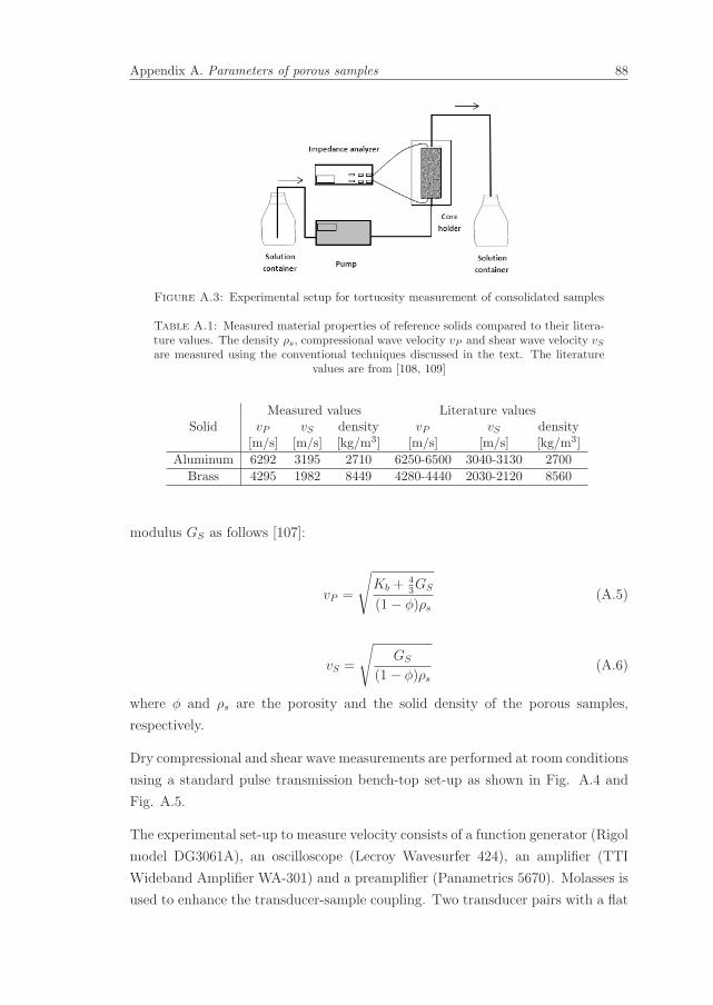
Appendix A. Parameters of porous samples 88
Figure A.3: Experimental setup for tortuosity measurement of consolidated samples
Table A.1: Measured material properties of reference solids compared to their litera-ture values. The density ρs, compressional wave velocity vP and shear wave velocity vSare measured using the conventional techniques discussed in the text. The literature
values are from [108, 109]
Measured values Literature valuesSolid vP vS density vP vS density
[m/s] [m/s] [kg/m3] [m/s] [m/s] [kg/m3]
Aluminum 6292 3195 2710 6250-6500 3040-3130 2700
Brass 4295 1982 8449 4280-4440 2030-2120 8560
modulus GS as follows [107]:
vP =
√Kb +
43GS
(1− φ)ρs(A.5)
vS =
√GS
(1− φ)ρs(A.6)
where φ and ρs are the porosity and the solid density of the porous samples,
respectively.
Dry compressional and shear wave measurements are performed at room conditions
using a standard pulse transmission bench-top set-up as shown in Fig. A.4 and
Fig. A.5.
The experimental set-up to measure velocity consists of a function generator (Rigol
model DG3061A), an oscilloscope (Lecroy Wavesurfer 424), an amplifier (TTI
Wideband Amplifier WA-301) and a preamplifier (Panametrics 5670). Molasses is
used to enhance the transducer-sample coupling. Two transducer pairs with a flat

Appendix A. Parameters of porous samples 89
Figure A.4: Schematic of the ultrasonic setup for measurement of frame and shearmodulus
Figure A.5: Photo of the ultrasonic setup. A sample (1) is clamped between twoidentical P-wave transducers (2) and (3). The sending transducer is connected to thefunction generater (4) through the voltage amplifier (5), while the receiving transducer
is connected to the oscilloscope (7) through the preamplifier (6).
Figure A.6: Compressional wave result for BereaUS5
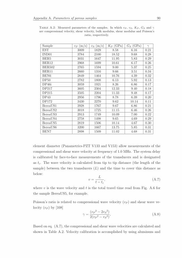
Appendix A. Parameters of porous samples 90
Table A.2: Measured parameters of the samples. In which vP , vS , KP , GS and γare compressional velocity, shear velocity, bulk modulus, shear modulus and Poisson’s
ratio, respectively.
Sample vP (m/s) vS (m/s) KP (GPa) GS (GPa) γ
EST 3009 1829 8.58 6.16 0.21
IND01 3784 2100 18.52 9.68 0.28
BER5 3031 1647 11.95 5.83 0.29
BER12 2968 1699 10.61 6.17 0.26
BER502 2765 1594 9.00 5.37 0.25
BER11 2660 1316 9.66 3.51 0.34
BEN6 2849 1464 10.76 4.39 0.32
DP50 2782 1808 6.13 5.92 0.13
DP46i 3059 1921 8.26 6.86 0.17
DP217 3605 2304 12.33 9.40 0.18
DP215 3505 2204 11.33 9.48 0.17
DP43 2956 1796 8.78 6.39 0.20
DP172 3430 2270 9.62 10.14 0.11
BereaUS1 2928 1767 9.67 6.86 0.21
BereaUS2 3018 1725 11.15 6.46 0.26
BereaUS3 2913 1749 10.09 7.00 0.22
BereaUS4 2758 1498 9.65 4.69 0.29
BereaUS5 2819 1506 10.14 4.67 0.30
BereaUS6 3200 1667 13.75 5.85 0.31
BEN7 2898 1509 11.02 4.68 0.31
element diameter (Panametrics-PZT V133 and V153) allow measurements of the
compressional and shear wave velocity at frequency of 1.0 MHz. The system delay
is calibrated by face-to-face measurements of the transducers and is designated
as tc. The wave velocity is calculated from tip to tip distance (the length of the
sample) between the two transducers (L) and the time to cover this distance as
below:
v =L
t− tc, (A.7)
where v is the wave velocity and t is the total travel time read from Fig. A.6 for
the sample BereaUS5, for example.
Poisson’s ratio is related to compressional wave velocity (vP ) and shear wave ve-
locity (vP ) by [108]
γ =(vP
2 − 2vS2)
2(vP 2 − vS2), (A.8)
Based on eq. (A.7), the compressional and shear wave velocities are calculated and
shown in Table A.2. Velocity calibration is accomplished by using aluminum and

Appendix A. Parameters of porous samples 91
copper blocks of different lengths. The compressional and shear wave velocities
for the reference solids are in agreement with the values from literature, as shown
in table A.1.
For each porous sample, the porosity and the solid density is known as shown
in Table 3.1 and Table 4.1. Therefore, the bulk modulus, shear modulus and
Poisson’s ratio for all samples are obtained and shown in Table A.2.

Appendix B
The equation to get the Stern
potential for 2:2 electrolytes
For 2:2 electrolytes, beside the deprotonation of silanol groups happening on the
silica surface as mentioned in eq.(1.1), the cation adsorption of divalent cations in
the solution happens as follows:
> SiOH0 +Me2+ ⇔ > SiOMe+ +H+ (B.1)
Therefore, there are three types of sites on the surface (one neutral >SiOH0 and
two negative >SiO− and >SiOMe+). The total mineral surface charge density Q0s
in C/m2 beomes
Q0s = −e(Γ0
SiO− − Γ0SiOMe+), (B.2)
where e is the elementary charge.
Based on the same arguments and notations described in [26] (see eq.(3)-11), the
surface site density of sites Γ0SiO− and Γ0
SiOMe are obtained as follows, respectively.
Γ0SiO− =
K(−)Γ0S
α0H+A
(B.3)
Γ0SiOMe+ = α0
Me2+KMe2+Γ
0S
α0H+A
(B.4)
where
A = 1 +K(−)α0
H+
+ α0Me2+
K(−)α0
Me2+, (B.5)
According to [26], the relationship between the activity of the ions α0H+ and α0
Me2+
at the mineral surface and the activity of the same those ions in the free electrolyte
93
Appendix B. The equation to get the Stern potential for 2:2 electrolytes 94
αfH+ and αf
Me2+ are related by
α0H+ = αf
H+e−eϕdkbT = αf
H+X2 = 10−pHX2, (B.6)
and
α0Me2+ = αf
Me2+e−2eϕdkbT = αf
Me2+X4 = CfX
4, (B.7)
with
X = e−eϕd2kbT , (B.8)
and Cf is the electrolyte concentration and ϕd is the Stern potential at the mineral
interface.
Using eqs. (B.3) to (B.8), the surface charge density is obtained as:
Q0s = −eΓ0
S
K(−) − CfKMeX4
K(−) + 10−pHX2 + CfKMeX4, (B.9)
The ionic strength, I, in the bulk solution is defined by
I =1
2
i=n∑i=1
z2iCfi (B.10)
where zi and Cfi are the valence and the concentration of ionic species i in mol/L,
respectively. Here, we ignore the reaction between pore water and atmospheric
CO2 which generates HCO3− and CO3
2− because this reaction is important only at
low electrolyte concentrations [26, 27]. Therefore, there are 4 types of ions in the
bulk solution (H+, OH−, Me2+, An2− and CH+=COH− and CMe2+=CAn2−=Cf ).
Now eq. (B.10) becomes
I =1
2{22CMe2+ + 22CAn2− + 12CH+ + 12COH−}
=1
2{8CMe2+ + CH+ + COH−} = 4Cf + 10−pH
(B.11)
The charge density in the diffuse layer is obtained in the same procedure as [26]
and defined by
Qs = 2χd
[2eCMe2+e
− 2eϕdkbT − 2eCAn2−e
2eϕdkbT + eCH+e
−−eϕd2kbT − eCOH−e
− eϕd2kbT
]
= 2χd
[2eCf (X
2 − 1
X2) + e10−pH(X − 1
X)
] (B.12)
Appendix B. The equation to get the Stern potential for 2:2 electrolytes 95
where χd is the Debye length already mentioned in chapter 1 and can be rewritten
in terms of the ionic strength
χd =
√ε0εrkbT
2e2I, (B.13)
Qs =
√b√I[Cf (X
2 − 1
X2) +
1
210−pH(X − 1
X)] (B.14)
b = 8× 10³ε0εrkbTN, (B.15)
At equilibrium conditions the charges on the mineral surface and in the diffuse
layer must be electrically neutral. That means
Qs +Q0s = 0 (B.16)
Putting eq. (B.9) and eq. (B.14) into eq. (B.16), we have
X6 +1
2
10−pH
Cf
X5 + [10−pH
CfKMe
+eΓ0
S
√I
Cf
√b]X4 +
1
2
10−2.pH
C2fKMe
X3
+K(−)
CfKMe
X2 +1
2
10−pHK(−)C2
fKMe
X − eΓ0SK(−)
√I
C2fKMe
√b
= 0
(B.17)
In eq. (B.17), we have used the same assumption mentioned in [26] that the
mineral surface potential (Stern potential) is such that 1/X << X or |ϕd| ≥ 20
mV. By using the numerical values of input parameters given in Table 3.3, we
see that odd terms are much smaller than even terms in eq. (B.17) (10−5 times
smaller) so odd terms can be ignored. Eq. (B.17) is written as
X6 + [10−pH
CfKMe
+eΓ0
S
√I
Cf
√b]X4 +
K(−)CfKMe
X2 − eΓ0SK(−)
√I
C2fKMe
√b
= 0 (B.18)
Putting t=X2, A= [ 10−pH
CfKMe+ eΓ0
S
√I
Cf
√b], B=
K(−)
CfKMeand C=− eΓ0
SK(−)
√I
C2fKMe
√b, eq. (B.18)
reduces to the cubic equation as follows:
t3 + At2 +Bt+ C = 0 (B.19)
We use a matlab code to solve a cubic equation eq. (B.19) and only take a
real solution. From that, the Stern potential and therefore the zeta potential are
obtained.

Bibliography
[1] B. Wurmstich and F. D. Morgan. Modeling of streaming potential responses
caused by oil well pumping. Geophysics, 59(1):46–56, 1994.
[2] R. F. Corwin and D. B. Hoover. The self-potential method in geothermal
exploration. Geophysics, 44(2):226–245, 1979.
[3] F. D. Morgan, E. R. Williams, and T. R. Madden. Streaming potential prop-
erties of westerly granite with applications. Journal of Geophysical Research,
94(B9):12.449–12.461, 1989.
[4] A. Revil and P. A. Pezard. Streaming electrical potential anomaly along
faults in geothermal areas. Geophysical Research Letters, 25(16):3197–3200,
1998.
[5] H. Mizutani, T. Ishido, T. Yokokura, and S. Ohnishi. Electrokinetic phe-
nomena associated with earthquakes. Geophys. Res. Lett., 3(2), 1976.
[6] M. Trique, P. Richon, F. Perrier, J.P. Avouac, and J.C.Sabroux. Radon
emanation and electric potential variations associated with transient defor-
mation near reservoir lakes. Nature, pages 137–141, 1999.
[7] A. A. Ogilvy, M. A. Ayed, and V. A. Bogoslovsky. Geophysical studies of
water leakages from reservoirs. Geophysical Prospecting, 17(1):36–62, 1969.
[8] A. Thompson, S. Hornbostel, J. Burns, and et al. Field tests of electroseismic
hydrocarbon detection. SEG Technical Program Expanded Abstracts, 2005.
[9] S.S. Haines, A. Guitton, and B. Biondi. Seismoelectric data processing for
surface surveys of shallow targets. Geophysics, 72(2):G1–G8, 2007.
[10] M. Strahser, L. Jouniaux, P. Sailhac, P.D. Matthey, and M. Zillmer. Depen-
dence of seismoelectric amplitudes on water content. Geophysical Journal
International, 187(2):1378–1392, 2011.
97

Bibliography 98
[11] S. Garambois and M. Dietrich. Seismoelectric wave conversions in porous
media: field measurements and transfer function analysis. Geophysics, 66
(2):1417–1430, 2001.
[12] P. Glover and M. Jackson. Borehole electrokinetics. The Leading Edge, 29
(6):724–728, 2010.
[13] http://www.hollandenvironment.com/soilreferences.html, .
[14] T. Paillat, E. Moreau, P.O.Grimaud, and G. Touchard. Electrokinetic phe-
nomena in porous media applied to soil decontamination. IEEE Transactions
on Dielectrics and Electrical Insulation, 7(5):693–704, 2000.
[15] C. Cameselle and K. R. Reddy. Development and enhancement of electro-
osmotic flow for the removal of contaminants from soils. Electrochimica Acta,
86:10–22, 2012.
[16] H. M Jacob and B. Subirm. Electrokinetic and Colloid Transport Phenom-
ena. Wiley-Interscience, 2006.
[17] R. J. Hunter. Foundations of Colloid Science. Oxford University Press, 1986.
[18] J. Lyklema. Fundamentals of Interface and Colloid Science. Academic Press,
1995.
[19] O. Stern. Zur theorie der electrolytischen doppelschist. Z. Elektrochem, 30:
508–516, 1924.
[20] T. Ishido and H. Mizutani. Experimental and theoretical basis of electroki-
netic phenomena in rock-water systems and its applications to geophysics.
Journal of Geophysical Research, 86:1763–1775, 1981.
[21] K. E. Butler. Seismoelectric effects of electrokinetic origin. PhD thesis,
University of British Columbia, 1996.
[22] H. Hase, T. Ishido, S. Takakura, T. Hashimoto, K. Sato, and Y. Tanaka.
Zeta potential measurement of volcanic rocks from aso caldera. Geophysical
Research Letters, 30(23):3197–3200, 2003.
[23] P. J. Heaney, C. T. Prewitt, and G. V. Gibbs. Silica. Mineralogical Society
of America, 29:606 pages, 1994.
[24] R. K. Iler. The Chemistry of Silica. John Wiley and Sons, New York, 1979.
Bibliography 99
[25] A. Revil and P. W. J. Glover. Theory of ionic-surface electrical conduction
in porous media. Physical Review B, 55(3):1757–1773, 1997.
[26] A. Revil, P. A. Pezard, and P. W. J. Glover. Streaming potential in porous
media 1. theory of the zeta potential. Journal of Geophysical Research, 104
(B9):20021–20031, 1999.
[27] P. W. J. Glover, E. Walker, and M.D. Jackson. Streaming-potential coef-
ficient of reservoir rock: A theoretical model. Geophysics, 77(2):D17–D43,
2012.
[28] R. J. Hunter. Zeta Potential in Colloid Science. Academic, New York, 1981.
[29] Jacob Israelachvili. Intermolecular and Surface Forces. Academic Press,
1992.
[30] Z. Zhui and M. N. Toksoz. Experimental measurements of the streaming
potential and seismoelectric conversion in berea sandstone. Geophysical
Prospecting, 61:688–700, 2013.
[31] R. G. Packard. Streaming potentials across glass capillaries for sinusoidal
pressure. The Journal of Chemical Physics, 21(2):303–307, 1953.
[32] S. Pride. Governing equations for the coupled electromagnetics and acoustics
of porous media. Physical Review B, 50(21):15678–15696, 1994.
[33] B. Nourbehecht. Irreversible thermodynamic effects in inhomogeneous media
and their applications in certain geoelectric problems. PhD thesis, MIT Press,
Cambridge, Mass, USA, 1963.
[34] A. Boleve, A. Crespy, A. Revil, F. Janod, and J. L. Mattiuzzo. Streaming
potentials of granular media: Influence of the dukhin and reynolds numbers.
J. Geophys. Res., B08204(6), 2007.
[35] J.T.G. Overbeek. Electrochemistry of the double layer: in Colloid Science,
Irreversible Systems, H. R. Kruyt, Ed. Elsevier, 1952.
[36] L. Jouniaux, M. L. Bernard, M. Zamora, and J. P. Pozzi. Streaming potential
in volcanic rocks from mount pelee. Journal of Geophysical Research B, 105
(4):8391–8401, 2000.
[37] S.S. Dukhin and V.N. Shilov. Dielectric Phenomena and the Double Layer
in Disperse Systems and Polyelectrolytes. John Wiley and Sons, New York,
1974.
Bibliography 100
[38] F. Reuss. Sur un nouvel effet de l’electricite galvanique. Memoires de la
Societe Imperiale de Naturalistes de Moscou, 2(6):327–336, 1809.
[39] Shuhuai Yao and Juan G. Santiago. Porous glass electroosmotic pumps:
theory. J. Colloid Interface Sci, 268(6):133–142, 2003.
[40] C.L. Rice and R. Whitehead. Electrokinetic flow in a narrow cylindrical
capillary. J. Phys. Chem., 69(11):4017–4024, 1965.
[41] R. Berg Robert. Reservoir Sandstones. Prentice Hall College Div, 1985.
[42] Zaki Bassiouni. Theory, Measurement, and Interpretation of Well Logs.
Henry L. Doherty Memorial Fund of AIME, Society of Petroleum Engineers,
1994.
[43] Abhijit Y. Dandekar. Petroleum Reservoir Rock and Fluid Properties. CRC
Press, 2013.
[44] P.J. Sides and J. D. Hoggard. Measurement of the zeta potential of planar
solid surfaces by means of a rotating disk. Langmuir, 20(26):11493–11498,
2004.
[45] J. D. Hoggard, P.J. Sides, and D. C. Prieve. Measurement of the streaming
potential and streaming current near a rotating disk to determine its zeta
potential. Langmuir, 21(16):7433–7438, 2005.
[46] J.R. Moore, S.D. Glaser, H.F Morrison, and G.M. Hoversten. The streaming
potential of liquid carbon dioxide in berea sandstone. Geophysical Research
Letters, 31(L17610), 2004.
[47] S. X. Li, D. B. Pengra, and P.Z.Wong. Onsager’s reciprocal relation and the
hydraulic permeability of porous media. Physical Review E, 51(6):5748–5751,
1995.
[48] S. Zeng, C. H. Chen, J. C. Mikkelsen, and J. G. Santiago. Fabrication and
characterization of electroosmotic micropumps. Sens. Actuators B, 79(2):
107–114, 2001.
[49] P. H. Nelson. Pore-throat sizes in sandstones, tight sandstones, and shales.
American Association of Petroleum Geologists Bulletin, 93(3):329–340, 2009.
[50] D. Bonn, S. Rodts, M. Groenink, R. Salima, N.S. Bonn, and P. Coussot.
Some applications of magnetic resonance imaging in fluid mechanics: com-
plex flows and complex fluids. Annu. Rev. Fluid Mech., 40:209–233, 2008.

Bibliography 101
[51] R. Brown. Connection between formation factor for electrical resistivity and
fluid solid coupling factor in biot’s equations for acoustic waves in fluid-filled
porous media. Geophysics, 45(8):1269–1275, 1980.
[52] F.B.J. Barends and P.M.P.C Steijger. Learned and Applied Soil Mechanics
- Tortuosity measurement and Its Spin-off to a new electrical conductivity
standard. Taylor and Francis, 2002.
[53] D. T. Luong and R. Sprik. Streaming potential and electroosmosis mea-
surements to characterize porous materials. ISRN Geophysics, Article ID
496352:8 pages, 2013.
[54] David R. Lide. CRC Handbook of Chemistry and Physics. CRC Press, 2004.
[55] D. H. Gray and J. K. Mitchell. Fundamental aspects of electro-osmosis in
soils. Journal of the Soil Mechanics and foundations Division, 93:209–236,
1967.
[56] G. E. Archie. The electrical resistivity log as an aid in determining some
reservoir characteristics. Petroleum Transactions of AIME, 146:54–62, 1942.
[57] P.N. Sen, C. Scala, and M. H. Cohen. A self-similar model for sedimentary
rocks with application to the dielectric constant of fused glass beads. Journal
of the Soil Mechanics and foundations Division, 46(5):781–795, 1981.
[58] P. W. J. Glover and E. Walker. Grain-size to effective pore-size transforma-
tion derived from electrokinetic theory. Geophysics, 74(1):E17–E19, 2009.
[59] L. Jouniaux and J.P. Pozzi. Permeability dependence of streaming potential
in rocks for various fluid conductivities. Geophysical Research Letters, 22(4):
485–488, 1995.
[60] Aristotelis Pagoulatos. Evaluation of multistage Triaxial Testing on Berea
sandstone. Degree of Master of Science, Oklahoma, 2004.
[61] F. Perrier and T. Froidefond. Electrical conductivity and streaming potential
coefficient in a moderately alkaline lava series. Earth and Planetary Science
Letters, 210:351–363, 2003.
[62] E. S. Sprunt, T.B. Mercer, and N.F. Djabbarah. Streaming potential from
multiphase flow. Geophysics, 59(5):707–711, 1994.
[63] A. Revil and H. Mahardika. Coupled hydromechanical and electromagnetic
disturbances in unsaturated porous materials. Water Resources Research,
49:744–766, 2013.
Bibliography 102
[64] A. Revil and P. W. J. Glover. Nature of surface electrical conductivity in
natural sands, sandstones, and clays. Geophysical Research Letters, 25(5):
691–694, 1998.
[65] D. T. Luong and R. Sprik. Permeability dependence of streaming potential
coupling coefficient. Submitted to Geophysics, 2014.
[66] S. R. Pride and F. D. Morgan. Electrokinetic dissipation induced by seismic
waves. Geophysics, 56(7):914–925, 1991.
[67] J. Vinogradov, M. Z. Jaafar, and M. D. Jackson. Measurement of streaming
potential coupling coefficient in sandstones saturated with natural and arti-
ficial brines at high salinity. Journal of Geophysical Research, 115(B12204):
doi:10.1029/2010JB007593, 2010.
[68] M. Z. Jaafar, J. Vinogradov, and M. D. Jackson. Measurement of streaming
potential coupling coefficient in sandstones saturated with high salinity nacl
brine. Geophysical Research Letters, 36(L21306):doi:10.1029/2009GL040549,
2009.
[69] L. Jouniaux and T.Ishido. Electrokinetics in earth sciences: A tutorial.
International Journal of Geophysics, 2012.
[70] S. L. Phillips, H. Ozbek, and R.J. Otto. Basic energy properties of elec-
trolytic solutions database. paper presented at Sixth International CODATA
Conference, 1978.
[71] P. N. Sen and P. A. Goode. Influence of temperature on electrical conduc-
tivity on shaly sands. Geophysics, 57(1):89–96, 1992.
[72] E. Bemer, O. Vincke, and P. Longuemare. Geomechanical log deduced from
porosity and mineralogical content. Oil and Gas Science and Technology, 59
(4):405–426, 2004.
[73] ILI Technical Committee. Indiana Limestone Handbook. Indiana Limestone
Institute of America, Inc., 2007.
[74] P.L. Churcher, P.R. French, J.C. Shaw, and L.L. Schramm. Rock properties
of berea sandstone, baker dolomite, and indiana limestone. SPE Interna-
tional Symposium, 1991.
[75] Alexei A. Tchistiakov. Physico-chemical aspects of clay migration and injec-
tivity decrease of geothermal clastic reservoirs. Proceedings World Geother-
mal Congress, 2000.

Bibliography 103
[76] Boris N. Kuvshinov. Shell international exploration and production, 2280ab
rijswijk, the netherlands. Shell International Exploration and Production,
2280AB Rijswijk, The Netherlands, 2012.
[77] Karel Heller. Department of geoscience and engineering, delft university of
technology. Department of Geoscience and Engineering, Delft University of
Technology, the Netherlands, 2012.
[78] Brian J. Kirby and E.F. Jr. Hasselbrink. Zeta potential of microfluidic sub-
strates: 1. theory, experimental techniques, and effects on separations. Elec-
trophoresis, 25:187–202, 2004.
[79] J.E. Dickens, J. Gorse, J.A. Everhart, and M. Ryan. Dependence of elec-
troosmotic flow in capillary electrophoresis on group i and ii metal ions.
Journal of Chromatography B, 657:401–407, 1994.
[80] Yongan Gu and Dongqing Li. The zeta potential of glass surface in contact
with aqueous solutions. Journal of Colloid and Interface Science, 226:328–
339, 2000.
[81] M. Lobbus, J. Sonnfeld, H.P. Van Leeuwen, W. Vogelsberger, and J. Lyk-
lema. An improved method for calculating zeta-potentials from measure-
ments of the electrokinetic sonic amplitude. Journal of Colloid and Interface
Science, 229:174–183, 2000.
[82] S. Datta, A.T. Conlisk, H.F. Li, and M. Yoda. Effect of divalent ions on
electroosmotic flow in microchannels. Mechanics Research Communications,
36:65–74, 2009.
[83] A. Sze, D. Erickson, L. Ren, and D. Li. Zeta-potential measurement using
the smoluchowski equation and the slope of the current–time relationship in
electroosmotic flow. Journal of Colloid and Interface Science, 261:402–410,
2004.
[84] B. Lorne, F. Perrier, and J. P. Avouac. Streaming potential measurements.
Journal of Geophysical Research, 104(B8):17.857–17.877, 1999.
[85] K. Guerra, K. Dahm, and S. Dundorf. Oil and gas produced water manage-
ment and beneficial use in the western united states. Science and Technology
Program Report, (157), 2011.
[86] P. M. Dove and J. D. Rimstidt. Silica-water interactions. Reviews in Min-
eralogy and Geochemistry, 29:259–308, 1994.
Bibliography 104
[87] M. Kosmulski and D. Dahlsten. High ionic strength electrokinetics of clay
minerals. Colloids and Surfaces, A: Physicocemical and Engineering Aspects,
291:212–218, 2006.
[88] P. J. Scales. Electrokinetics of the muscovite mica-aqueous solution interface.
Langmuir, 6:582–589, 1990.
[89] L. J. Criscenti and D. A. Sverjensky. The role of electrolyte anions (ClO4−,
NO4− , and Cl− ) in divalent metal (M2+ ) adsorption on oxide and hydroxide
surfaces in salt solutions. American Journal of Science, 299:828–899, 1999.
[90] http://gtresearchnews.gatech.edu/newsrelease/NEARCRIT.html, .
[91] R. Hidalgo-Alvarez, A. Delgado, J. Callejas, and F. Gonzalez-Caballero.
Electrophoretic behaviour of calcium oxalate monohydrate in liquid mix-
tures. Colloid and Polymer Science, 263:941–947, 1985.
[92] Francisco Jose Rubio Hernandez. Dependence of the electrophoretic coeffi-
cient of polystyrene model colloids on the solvent composition. Journal of
Colloid and Interface Science, 203:208–213, 1998.
[93] Roque Hidalgo-Alvarez, Francisco Javier de las Nieves, and Gerardo Pardo.
Concentration dependence of electrokinetic transport coefficients of non-
aqueous binary mixtures through weakly charged porous plugs. Journal
of the Chemical Society, Faraday Transactions 1: Physical Chemistry in
Condensed Phases, 81:609–619, 1998.
[94] M.L. Srivastava and S.N. Lal. Electro-kinetic transport of acetone, water
and their binary mixtures. Colloid and Polymer Science, 258:877–882, 1980.
[95] Chris Stenland and B. Montgomery Pettitt. Binary-solution critical opales-
cence: Mole fraction versus temperature phase diagram. Journal of Chemical
Education, 72(6):560–564, 1995.
[96] E. S.R Gopal. Critical opalescence. Resonance, 5(4):37–45, 2000.
[97] N. Hafaiedh, A. Toumi, and M. Bouanz. Dynamic viscosity study of binary
mixtures triethylamine + water at temperatures ranging from (283.15 to
291.35) k. Journal of Chemical and Engineering Data, 54(8):2195–2199,
2009.
Bibliography 105
[98] N. Hafaiedh, A. Toumi, and M. Bouanz. Electrical conductivity investi-
gation of diluted potassium chloride solutions in binary mixture triethy-
lamine–water near its consolute point k. Fluid Phase Equilibria, 305(305):
185–191, 2011.
[99] J. Hamelin, T.K. Bose, and J. Thoen. Critical behavior of the dielectric
constant in the triethylamine-water binary liquid mixture: Evidence of an
intrinsic effect. Physical Review E, 53(1):779–784, 1996.
[100] A. Toumi, N. Hafaiedh, and M. Bouanz. Study of the transport properties
of the critical binary mixture triethylamine – water with an ionic impurity.
Ukrainian Journal of Physics, 56(8):816–823, 2011.
[101] L. Grunberg and A. H. Nissan. Mixture law for viscosities. Nature, 164(16):
799–802, 1949.
[102] F. Kohler and O. K. Rice. Coexistence curve of the triethylamine-water
system. Journal of Chemical Physics, 26(6):1614–1618, 1957.
[103] C. Pepin, T. K. Bose, and J. Thoen. Evidence for an intrinsic refractive-
index anomaly in a critical binary liquid mixture. Physical Review Letters,
60(24):2507–2510, 1988.
[104] G. P. Furrow and S. C. Greer. Critical behavior of the density, heat capacity,
and refractive index for triethylamine + water. Journal of Chemical Physics,
79(7):3474–3481, 1983.
[105] G. Mavko, T. Mukerj, and J. Dvorkin. The Rock Physics Handbook - Tools
for Seismic Analysis in Porous Media. Cambridge University Press, 2003.
[106] Osborne Reynolds. An experimental investigation of the circumstances which
determine whether the motion of water shall be direct or sinuous, and of the
law of resistance in parallel channels. Philosophical Transactions of the Royal
Society, 174:935–982, 1883.
[107] C.J. Wisse. On frequency dependence of acoustic waves in porous cylinders.
PhD thesis, Delft University of Technology, the Netherlands, 1999.
[108] A. Kumar, T. Jayakumar, B. Raj, and K.K Ray. Correlation between ul-
trasonic shear wave velocity and poisson’s ratio for isotropic solid materials.
Acta Materialia, 51:2417–2426, 2003.
[109] T. Kundu. Ultrasonic Nondestructive Evaluation: Engineering and Biologi-
cal Material Characterization. CRC Press, New York, USA, 2003.

Summary
This thesis presents the PhD research on electrokinetics in porous media. Elec-
trokinetic phenomena are induced by the relative motion between a fluid and a
solid surface and are directly related to the existence of an electric double layer
between the fluid and the solid grain surface. Electrokinetic phenomena consist of
several different effects such as streaming potential, electroosmosis, electrophore-
sis. The thesis only focuses on streaming potential and electroosmosis effects in
porous media. Below is the summary of the research.
Chapter 1 introduces the applications of electrokinetic phenomena in geophysical
applications and environmental applications, physical chemistry of the interface
between solid grains and fluids, and the theoretical backgrounds of streaming po-
tential and electroosmosis effects happening in porous media saturated by fluids.
This chapter also presents definitions of microstructure parameters used through-
out the thesis to describe porous media such as the porosity, permeability, tortu-
osity, formation factor and solid density. Some interesting ideas that deserve more
research are also shown in this chapter.
The coupling coefficients of conversion between seismic wave and electromagnetic
wave depend strongly on the fluid conductivity, porosity, permeability, formation
factor, pore size, zeta potential of porous media and other properties of the rock
formation. Therefore, determining these parameters is very important in studying
electrokinetics in general and to model seismoelectric and electroseismic conver-
sions. Chapter 2 presents an approach to characterize porous media using dc
measurements of streaming potential and electroosmosis effects. The experimen-
tal results are in good agreement with the theoretical model. In particular, the
approach works in particular well for very small pore samples.
Permeability is one of the most important physical parameters to describe reser-
voir rocks. In theory, the streaming potential coupling coefficient depends not
only on the zeta potential but also on the permeability of the rocks that partially
107

Summary 108
determines the surface conductivity of the rocks. However, in practice it is hard
to show the permeability dependence of streaming potential coupling coefficients
because of the variation of zeta potential from sample to sample. In chapter 3, we
study permeability dependence of streaming potential including the effects of the
variation of the zeta potential and surface conductance due to the difference in
mineral compositions between samples. We perform measurements on 12 consol-
idated samples including natural and artificial samples saturated with 7 different
NaCl solutions to determine streaming potential coupling coefficients. The re-
sults have shown that the coupling coefficients strongly depend on permeability
of the samples for low fluid conductivity. When the fluid conductivity is larger
than 0.13 S/m (0.01M NaCl solution), the coupling coefficient is independent of
permeability. This observation is quantitatively explained by a theoretical model.
In chapter 2 and chapter 3, the streaming potential coupling coefficient is experi-
mentally measured and the zeta potential is deduced from that. That is the most
commonly used approach to obtain the coupling coefficient and the zeta potential
of electrolyte saturated rocks. Glover et al. [27] developed a theoretical model to
calculate the zeta potential and streaming potential coefficient of reservoir rocks
and other porous media. The authors have compared the theoretical results to an
experimental data set from available published data. The comparison shows that
the theoretical model can reproduce the main features of the experimental data.
However, the existing experimental data sets are based on samples with dissim-
ilar fluid conductivity, pH of pore fluid, temperature and sample compositions.
All those dissimilarities may cause the observed deviations. To critically assess
the model, in chapter 4 we have carried out streaming potential measurement as
a function of electrolyte concentration and temperature for a set of well-defined
consolidated samples. The results show that the theoretical model is not in good
agreement with the experimental observations when varying the electrolyte con-
centration. If we use a modified model in which the zeta potential is considered
to be constant over the electrolyte concentration, the model fits the experimental
data well. Also for temperature dependence, the comparison shows that the the-
oretical model is not fully adequate to describe the experimental data, but does
describe correctly the increasing trend of the coupling coefficient as function of
temperature.
In chapter 2, chapter 3 and chapter 4, all streaming potential measurements are
carried out for NaCl solution only. In reality most reservoir rocks are saturated
or partially saturated by natural waters that normally contain monovalent and
divalent electrolytes. Therefore, in chapter 5 we study the dependence of the zeta

Summary 109
potential on types of electrolytes systematically using streaming potential mea-
surements. The experimental results show that the coupling coefficient and the
zeta potential depend not only on the mineral compositions but also on types of
electrolyte (mainly types of cation). The experimental results also show that the
zeta potential for monovalent electrolytes is higher than that for divalent elec-
trolytes. The reservoir rocks made of silica have the highest zeta potentials when
saturated by the same type of electrolyte. The experimental results are explained
by theoretical models. For monovalent electrolytes, we use a theoretical model
that is available in literature. For divalent electrolytes, we develop another model
to explain the experimental data. The results shows that the theoretical models
can explain the main behavior of the zeta potential against types of electrolyte
and types of sample. For a given electrolyte, the difference in the zeta potential
can be explained by the difference in the surface site density and disassociation
constant for different kinds of porous rocks (mineral compositions). For a given
sample, the difference in the zeta potential can be explained by the difference in
binding constants of cations and in types of cations.
In previous chapters, aqueous electrolytes have been used to study the streaming
potential. In chapter 6, we carry out the streaming potential measurements for
an artificial sandstone sample saturated with a binary mixture of triethylamine-
water with three different mass fractions. The results show that the zeta potential
changes with compositions of TEA and temperature. Interestingly, an anomaly
of the zeta potential has been predicted near the critical point for the critical
composition. Therefore, there may be an anomalous change of the electric double
layer and the Debye length near the critical point.
In Appendix A, we present the approaches and setups to determine parameters of
porous media such as the porosity, density of grains, tortuosity, formation factor
and steady-state permeability. Those parameters are already used and mentioned
in previous chapters. In addition, we also determine the frame and shear modulus
of the consolidated samples.
In Appendix B, we derive an expression to calculate the zeta potential for divalent
electrolytes that is applied in chapter 5 to explain the experimental data.

Samenvatting
Dit proefschrift presenteert het onderzoek naar elektrokinetica in poreuze materi-
alen gedaan tijdens mijn promotie. Elektrokinetische fenomenen worden veroorza-
akt door de relatieve beweging van een vloeistof langs een vast oppervlak en is
direct gerelateerd aan de elektrische dubbellaag tussen de vloeistof en vaste stof.
Elektrokinetische fenomenen bestaan uit verschillende effecten, bijvoorbeeld: het
stromingspotentiaal, elektro-osmose en elektroforese. Deze dissertatie focust op
het stromingspotentiaal en elektro-osmotische effecten in poreuze materialen. Hi-
eronder volgt een samenvatting van het onderzoek.
Hoofdstuk 1 introduceert de toepassing van elektrokinetische fenomenen in de
geofysica , milieu wetenschappen, fysische chemie van het oppervlak tussen een
poreuze vaste stof en een vloeistof en de theoretische achtergrond van het stromings
potentiaal en elektro-osmotische effecten die plaats vinden in poreuze materialen
verzadigd met een vloeistof. Dit hoofdstuk behandelt tevens de microstructuur pa-
rameters die gebruikt worden in deze dissertatie om poreuze materialen te beschri-
jven zoals porositeit, permeabiliteit, tortuosity, formatie factor en dichtheid van
de vaste stof. Een aantal interessante ideeie meer onderzoek vereisen worden ook
behandeld in dit hoofdstuk.
De koppelingscoefficient voor conversie tussen seismische golven en elektromag-
netische golven hangt sterk af van de elektrische geleiding van de vloeistof, de
porositeit, de permeabiliteit, de formatie factor, de ruimte tussen de korrels, de
zeta potentiaal van poreuze materialen en andere eigenschappen van het gesteente.
Daarom is het bepalen van deze parameters zeer belangrijk in de elektrokinetica en
om seismo-elektrische en elektro-seismische conversie te modelleren. Hoofdstuk 2
behandelt een methode om poreuze materialen te karakteriseren aan de hand van
dc metingen van de stromings potentiaal en elektro-osmotische effecten. De ex-
perimentele resultaten zijn in goede overeenstemming met het theoretische model.
De methode werkt in het bijzonder goed voor materialen met kleine ruimtes tussen
de korrels.
111
Samenvatting 112
Permeabiliteit is een van de belangrijkste fysische parameters voor het beschrijven
van reservoir gesteente. In theorie hangt de stromingspotentiaal koppeling coef-
ficient niet alleen van de zeta potentiaal af, maar ook van de permeabiliteit van
het gesteente wat gedeeltelijk de oppervlakte geleiding van het gesteente bepaalt.
Echter, in de praktijk is het moeilijk om de permeabiliteits afhankelijkheid van
de koppeling coefficient te bepalen, omdat de zeta potentiaal varieert van sample
to sample. In hoofstuk 3 bestuderen we de permeabiliteit afhankelijkheid van de
stromingspotentiaal, waaronder ook het effect van variatie in de zeta potentiaal en
oppervlakte geleiding door wisselende mineraal composities tussen samples. We
doen metingen aan 12 samples, waaronder natuurlijke en kunstmatige samples
verzadigd met 7 verschillende NaCl oplossingen om de koppeling coefficient te
bepalen. De resultaten laten zien dat de koppeling coefficient sterk afhangt van de
permeabliteit van de samples voor lage vloeistof geleiding. Voor vloeistof geleiding
groter dan 0.13 S/m (0.01M NaCl solution) is de koppeling coefficient onafhanke-
lijk van de permeabiliteit. Deze observatie is in kwantitatieve overeenstemming
met een theoretisch model.
In hoofdstuk 2 en 3 wordt de koppeling coefficient experimenteel gemeten en wordt
de zeta potentiaal hiervan afgeleid. Dit is de meest gebruikelijke aanpak om de
koppeling coefficient en de zeta potentiaal van gesteente verzadigd met elektrolyten
te bepalen. Glover et al. [27] ontwikkelde een theoretisch model om de koppeling
coefficient en zeta potentiaal van reservoir gesteente en andere poreuze materialen
te berekenen. De auteuren van dat werk vergelijken hun theoretische voorspellin-
gen met experimentele data uit reeds gepubliceerd werk. De vergelijking laat zien
dat het theoretische model de belangrijkste eigenschappen van de experimentele
data kan reproduceren. Echter, de bestaande experimentele data is gebaseerd op
samples met verschillende vloeistof geleiding, pH van de vloeistof, temperatuur
en sample compositie. Al die verschillen zijn mogelijk de oorzaak van de afwijk-
ing tussen theorie en experiment. Om het model kritisch te kunnen beoordelen
beschrijven we in hoofdstuk 4 metingen van de stromings potentiaal als functie
van elektrolyt concentratie en temperatuur van goed gedefinieerde geconsolideerde
samples. Als we een aangepast model gebruiken waarin de zeta potentiaal con-
stant is over de elektrolyt concentratie, fit de theorie de data goed. Een vergelijking
van experimentele data en theorie voor de temperatuur afhankelijkheid laat zien
dat het model niet volledig adequaat is, maar dat het model de stijging van de
koppeling coefficient als functie van de temperatuur goed beschrijft.
In de hoofdstukken 2, 3 en 4 zijn alle metingen uitgevoerd met NaCl oplossingen.
In de realiteit zijn de meeste reservoir gesteente verzadigd of gedeeltelijk verzadigd

Samenvatting 113
met natuurlijk water dat monovalente en divalente elektrolyten bevat. Daarom
beschrijven we in hoofdstuk 5 systematische metingen van de zeta potentiaal voor
verschillende elektrolyten gebruikmakend van de stromingspotentiaal. De experi-
mentele resultaten laten zien dat de zeta potentiaal voor monovalente elektrolyten
hoger is dan voor divalente elektrolyten. De reservoir gesteente gemaakt van sili-
cium hebben het hoogste zeta potentiaal wanneer verzadigd met dezelfde soort
elektrolyt. De experimentele resultaten worden uitgelegd aan de hand van the-
oretische modellen. Voor monovalente elektrolyten gebruiken we een theoretisch
model uit de literatuur. Voor divalente elektrolyten ontwikkelen we een andere
methode om de experimentele data te verklaren. De resultaten laten zien dat de
theoretische modellen het gedrag van de zeta potentiaal voor verschillende type
elektrolyten en samples in grote lijnen kunnen verklaren. Voor een gegeven elek-
trolyt kan het verschil in zeta potentiaal worden verklaard door het verschil in op-
pervlakte dichtheid en disassociatie constante voor verschillende soorten poreuze
gesteente (mineraal compositie). Voor een gegeven sample kan het verschil in zeta
potentiaal worden uitgelegd door het verschil in bindingsconstante voor verschil-
lende kationen.
In de voorgaande hoofdstukken gebruikten we elektrolyten opgelost in water om de
stromingspotentiaal te bestuderen. In hoofdstuk 6 voeren we experimenten uit om
de stromingspotentiaal te bepalen in kunstmatige zandstenen verzadigd met een
binaire mix van triethylamine-water met drie verschillende massa concentraties.
De resultaten laten zien dat de zeta potentiaal verandert met compositie van TEA
en temperatuur. Een interessante anomalie in de zeta potentiaal is aangetoond
bij het kritische punt voor de kritische compositie. Daarom is er wellicht een
afwijkende verandering in de elektrische dubbellaag en de Debye lengte in de buurt
van het kritische punt.
In Appendix A presenteren we de aanpak en experimentele opstelling gebruikt
om de karakteristieke parameters van poreuze materialen te bepalen zoals de
porositeit, dichtheid van de korrels, tortuosity, formatie factor en steady-state
permeabiliteit. Deze parameters zijn al genoemd en gebruikt in de voorgaande
hoofdstukken. Daarbij hebben we ook de compressie modulus van het poreuze
frame en de schuifmodulus bepaald voor geconsolideerde samples.
In Appendix B lijden we een uitdrukking af om de zeta potentiaal voor divalente
elektrolyten te berekenen, die wordt toegepast in hoofdstuk 5 om de experimentele
data te verklaren.

Publications
1. D. T. Luong and R. Sprik, ”Streaming Potential and Electroosmosis Measure-
ments to Characterize Porous Materials”, ISRN Geophysics, vol. 2013, Article ID
496352, 8 pages, 2013. doi:10.1155/2013/496352
2. D. T. Luong and R. Sprik, ”Examination of a Theoretical Model of Streaming
Potential Coupling Coefficient”, International Journal of Geophysics, vol. 2014,
Article ID 471819, 12 pages, 2014. doi:10.1155/2014/471819
3. D. T. Luong and R. Sprik, ”Permeability dependence of streaming potential
in porous media”, Geophysics (undergoing review).
4. D. T. Luong and R. Sprik, ”Zeta potential of porous rocks in contact with
monovalent and divalent electrolyte aqueous solutions” ( in preparation).
5. D. T. Luong and R. Sprik, ”Streaming potential with binary mixture - Tri-
ethylamine and water near the demixing phase transition” (in preparation).
114

Acknowledgements
I want to take this opportunity to thank all people who turned my dream into a fact
during more than 4 years in Amsterdam.
First and foremost, I would like to express my special appreciation and thanks to my
supervisor, Dr. Rudolf Sprik, you have been a big mentor for me. You always listened
to me to understand what I really needed and guided me to overcome all the problems
and difficulties I encountered during my PhD. Without your support, I could not have
done what I was able to do. Dear Rudolf, again thank you very much for accepting me
as a PhD student at University of Amsterdam, being patient with me and showing me
how to do research.
Additionally, I am very grateful to my promotor, Prof. Dr. Daniel Bonn for helping and
providing me both academic guidance and financial support. Without your help and
support, pursuing a PhD degree would have been much more difficult for me. Thank
you very much for understanding. I will always remember what you asked me sometimes
”Are you hungry ?” and of course I could not say ”No”.
I would like to thank Dr. Peter schall and Dr. Noushine Shahidzadeh for nice conversa-
tions and fruitful comments you gave me in the group meetings.
I would also like to thank my committee members for serving as my committee members
and their helpful comments and suggestions that helped me improve my thesis.
I would be remiss if I did not acknowledge Ngo Ngoc Ha for introducing me to Rudolf
Sprik and helping me when I fist came to Amsterdam.
Many thanks are given to my dear colleagues in the Soft Matter group of the Van der
Waals-Zeeman Institute for their helps and nice talks: Daniel, Dmitry, Bart, Christiaan,
Henri, Sareh, Triet, Mehdi, Julie, Odile, Marius, Marthe, Jose, Duc, Anh, Maureen,
Janaina, Rojman, Dominik, Nick, Bruce, Katie, Mounir, Kinga, Oleg, Yasser and San-
dra.
A special thanks to Dmitry, Bart and in particular Daniel Miedema for reading my
papers, giving me very helpful comments, having very nice talks in ”tijd voor een bakkie”
and etc. Christiaan, thank you very much for giving me nice suggestions and useful
discussion about building the experimental set-up.
I would also like to thank Daniel Miedema and Marius for being my paranymphs. I am
very happy to have your support on the 9th of October which will stick to my memory
forever.
115

Acknowledgements 116
This thesis would have been impossible without the help of Rita, Ineke, Luuk, Natalie,
Anne-Marieke, Yocklang and Joost. Thanks a lot for your willingness to always help me.
A special thanks goes to Rita, Luuk and especially Ineke for your kindness, supports
and nice talks of course.
I would also like to thank Christel van der Storm, Truc Ngo, Arend van Leeuwen, Niels
Molenaar, Erith Boniel for helping me deal with paper work, visa, residence permit,
housing etc.
In the Institute of Physics there are some people I have met during my PhD, with whom
I have had nice talks in social gatherings: coffee/tea/beer etc. A special thanks is given
to Rens, Kat, Richard, Chris, Elinore, Tuan, Chung, Bay, Dr. Anne de Visser, Prof.
Tom Gregorkiewicz and Prof. Mark Golden.
I would also like to thank all people in the workshop of the University of Amsterdam,
especially Hans Ellermeijer, Hans Agema, Wim van Aartsen, Joost Overtoom, Gert Jan
Bon, Harry Beukers and Ron Manuputy for the countless times they helped me with
supplies in building the set-ups.
I would like to thank Prof. Kees Wapenaar, Prof. Evert Slob and Niels Grobbe for
fruitful discussions and suggestions in periodic meetings in Shell oil company, Technical
University of Delft (TU Delft) and University of Amsterdam. I would also like to thank
Karel Heller (TU Delft) for showing me how to measure tortuosity of porous samples
and giving me suggestions to improve the set-ups.
Many thanks are given to people of the Shell Oil Company and the Foundation for
Fundamental Research on Matter (FOM) in The Netherlands for getting me involved in
the project. A special thanks is given to Boris N. Kuvshinov (Shell) for providing me
the samples.
I would like to thank Ministry of Education and Training (MOET) of Vietnam for
granting me a scholarship to study abroad. A special thanks is given to Tran Thi Nga
(MOET) for her helps with paper work, quick responds to my queries and etc. I would
also like to thank Water Resources University (WRU) for facilitating my study and the
supports. I am also very grateful to my colleagues at Physics Division (WRU) for their
helps and taking over the tasks I left behind during my PhD.
I would like to thank all of my Vietnamese friends in the Netherlands for your helps and
very nice time we had in parties, barbecue, new year, football, tennis, table tennis and
etc.
A special thanks to my family. Words can not express how grateful I am to my parents
for all of their sacrifices and their enduring love for me. I would also like to thank my

Acknowledgements 117
parents-in law, my brothers, my grandparents, my uncles, my aunts, my brother in law
and my sister in law for their supports.
Last but not least, I would like express my deep appreciation to my wife, Tuoi and my
children, Duy Vinh and Khoi Nguyen who have supported me constantly and always
shared the hard moments with me. Thanks for loving me and for being there any single
moment I need.

Top Related