


Languages
Pages
Legal


Using Random Numbers
Modeling and Simulation of Biological Systems 21-366B
Lecture 2-3
A textbook on probability:G.R. Grimmett and D.R. Stirzaker
Probability and Random Processes OXFORD
MotivationWhy randomness?
It seems to be present everywhere.It may be a useful approach to simplify modelsIt may address our limited knowledge about a systemIt may be useful to express variability in a population…..
Examples:
stock market behavior, individual stocks and averagesmotion of microscopic particles in waterbacterium trajectory in a fluidAffinity maturation of B cell antibodiestraffic behavior….

Cont.
Randomness may be in the structure (spatial) or dynamics
Even deterministic models may exhibit an apparently random behavior
Atomistic models of fluids and solids (movies later)
Insufficient sampling of a phenomenon (movies later)
Grain boundaries in polycrystalline materials (pictures)

Cont.
Large networks of biochemical reactions seem to have randomness in its connectivity
metabolic networksprotein-protein interactions
Internet connectivity
……

Random Number Generation
Uniform distribution
MATLAB function:
rand : gives a single number in (0,1), distributed uniformly in [0,1]
rand(n,1) : give a vector of n numbers, …
rand(n) : gives a n by n matrix ….

Random Variables Attaining a few values
Let a random variable attain two values,
To generate such a random variable:
Later we will regard the event X=1 as a jump.

Basic MATLAB (use MATLAB help!!)
Vectors:v = ones(n,1); %generate a row vector of onesa = v’; % a is a column vector of onesb = zeros(n,1); % a row vector of zeroesv = [1:10]; % a vector [1 2 3 .. 10]a = [1 2 3; 4 5 6]; % a 2 by 3 matrix
Matrix Operations:A = B + C; A = B – C;A*v; % v must be a column vector
Loops:for i=1:10
….end

more MATLAB commands
C = fix(10*rand(3,2)); %create a 3 by 2 matrix, of integers 0->9
fix: %round toward zeroplot(x); % plot the values in a vector xbar(x); % create a bar graph form a vectorsum(x); %hist(x); % create a histogram from the values of xhist(x,n); % histogram with n binsx = rand(n,1); % a vector of n random numbers U[0,1]Ind = find(x>=0.5); % ind is an array of indices satisfying ….clear all; % clear memory

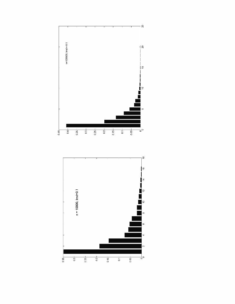
Studying Jump Time Intervals
%jumpTime.m% find the distribution of jump time intervalsn=10000;Lamd = 0.1;r = rand(n,1);Ind = find(r<=Lamd); %Ind is an array of indices at which jumps will
%occurfor i=1:length(Ind)-1
j(i) = Ind(i+1)-Ind(i);endv = hist(j,20); %construct histogram of the j valuesw = v/sum(v); %normalizebar(w);

Normal distribution:
MATLAB function
randn : a single random numberrandn(n,1) : n vector of n random numbersrandn(n) : an n by n matrix of random numbers
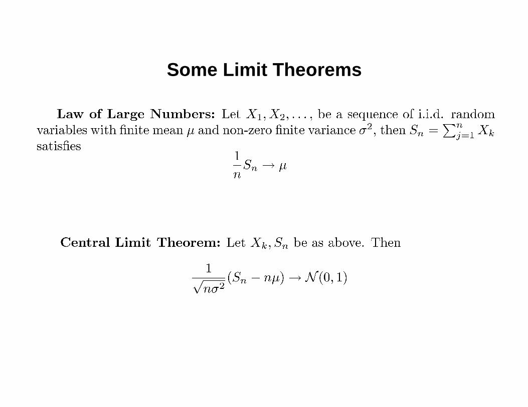
Some Limit Theorems
Converges of Averages (LLN)
% average.mn=1000;y = rand(n,1);s(1)=y(1);for i=2:n
s(i) = s(i-1)+y(i);endfor i=2:n
s(i) = s(i)/i;endplot(s);

Behavior of Averages (CLT)% CLT.mn=1; s = zeros(n,1);c = ['r','g','b','c','m','y','k'];for l=1:20000
y = rand(n,1);s(1)=y(1);for i=2:n
s(i) = s(i-1)+y(i);endz(l) = (s(n)-0.5*n)/sqrt(n);
endm=25;w=hist(z, m);v=linspace(-0.5,0.5,m);bar(v,w/m);

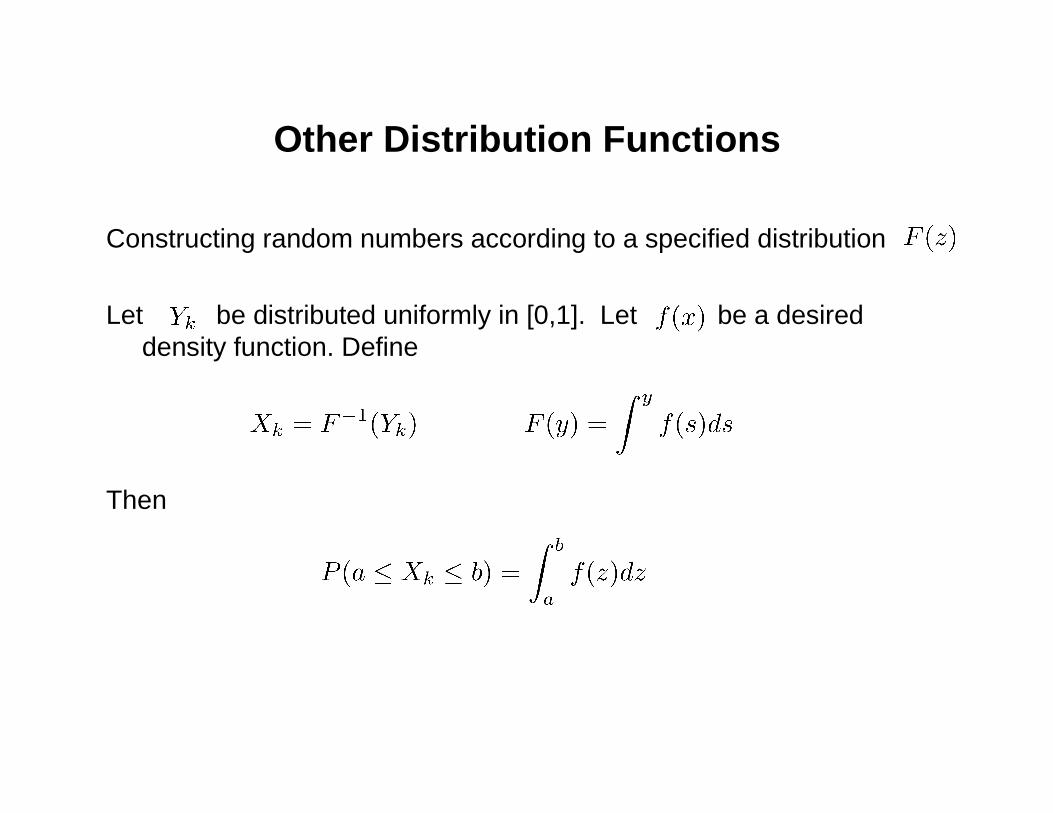
Other Distribution Functions
Constructing random numbers according to a specified distribution
Let be distributed uniformly in [0,1]. Let be a desired density function. Define
Then
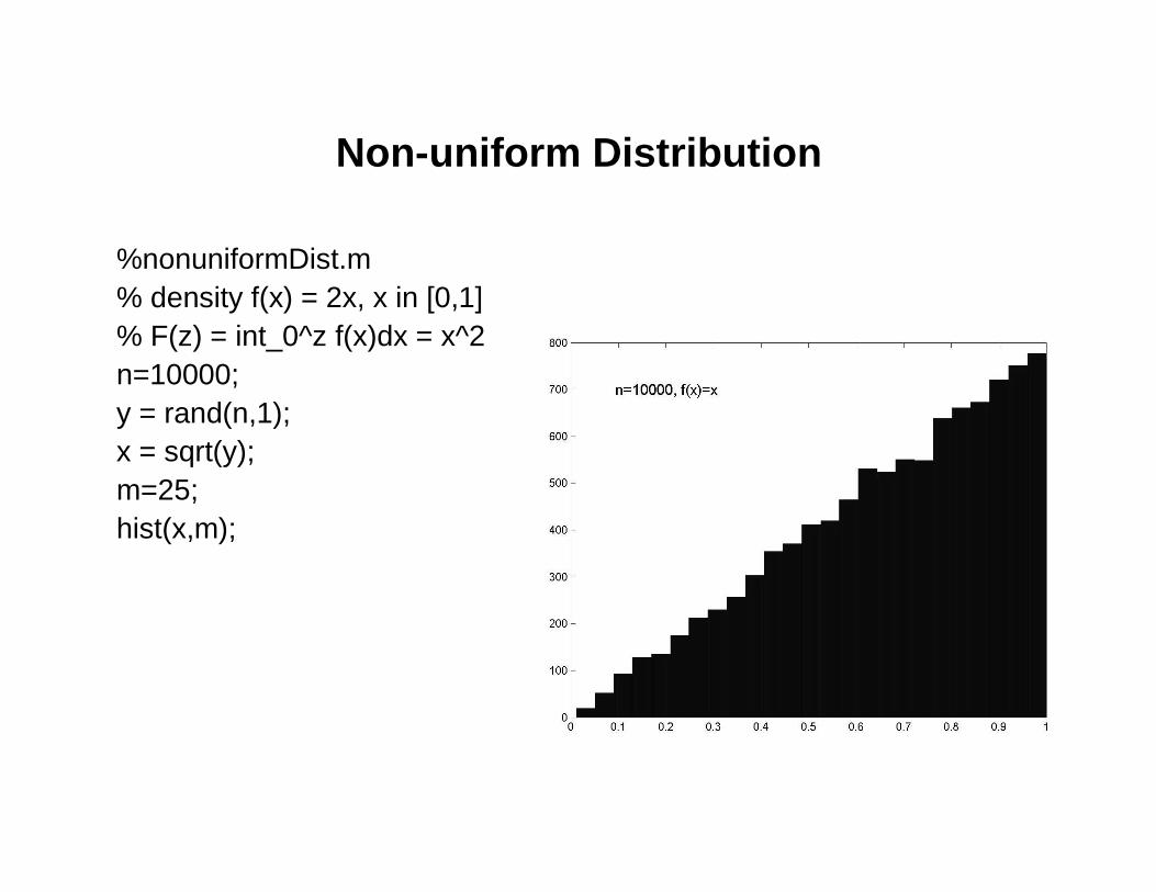
Non-uniform Distribution
%nonuniformDist.m% density f(x) = 2x, x in [0,1]% F(z) = int_0^z f(x)dx = x^2n=10000;y = rand(n,1);x = sqrt(y);m=25; hist(x,m);
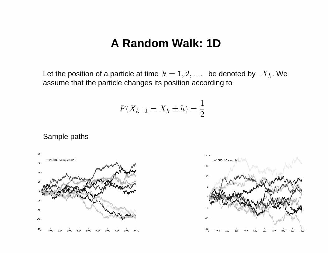
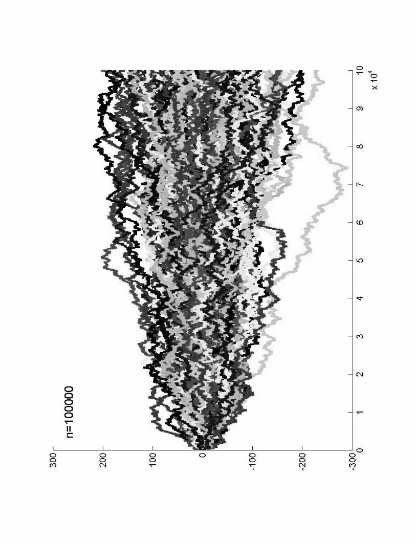
A Random Walk: 1D
Let the position of a particle at time be denoted by . We assume that the particle changes its position according to
Sample paths

MATLAB code
% randWalk1D.m% (symmetric) random walk in 1Dn=100000; %number of stepsfigure;hold on;c = ['r','g','b','c','m','y','k'];for l=1:100
%x = (rand(n,1) - 0.5*ones(n,1)); %uniformly distributed jumps%x = randn(n,1); % normal
%jumps are +-1x = (rand(n,1) - 0.5*ones(n,1));indP = find(x>0);indM = find(x<=0);x(indP) = 1;x(indM) = -1;z = zeros(n,1);for i=2:n
z(i) = z(i-1)+ x(i);endplot(z,'Color', c(mod(l,7)+1),'LineWidth',2);
end
Random Walk: 2D
Let the position of a particle at time be denoted by We assume that the particle changes its position according to
Sample paths:
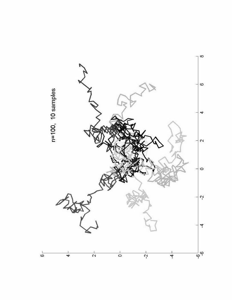


randWalk2D.m%random walk in 2D, uniformly dist jumps%random walk in 2D, uniformly dist jumpsn=100000;n=100000;figure;figure;hold on;hold on;c = ['c = ['r','g','b','c','m','y','kr','g','b','c','m','y','k'];'];for l=1:10for l=1:10
x = (rand(n,1) x = (rand(n,1) -- 0.5*ones(n,1));0.5*ones(n,1));y = (rand(n,1) y = (rand(n,1) -- 0.5*ones(n,1)); 0.5*ones(n,1)); z1 = zeros(n,1);z1 = zeros(n,1);z2 = zeros(n,1);z2 = zeros(n,1);for i=2:nfor i=2:n
z1(i) = z1(iz1(i) = z1(i--1) + 1) + x(ix(i););z2(i) = z2(iz2(i) = z2(i--1) + 1) + y(iy(i););
endendplot(z1,z2,'Color', plot(z1,z2,'Color', c(mod(l,7)+1),'LineWidth',2);c(mod(l,7)+1),'LineWidth',2);endend
Can change the jump Can change the jump distribution to be normal distribution to be normal ((randnrandn), ),
Or just +=1 jumpsOr just +=1 jumps
Code for this is on the web Code for this is on the web page!page!

Some Questions
Starting from the origin, what is the probability that a particle will reach a specified location (area), during a given time interval?
1. What is the probability of a molecule to reach the nucleus using random walk, starting from the membrane?
2. Can a macrophage find a bacterium, using just a random walk?
Starting from the origin, what is the average time that it takes a particle to reach a specific location (area)?
1. How long on the average it takes a signaling protein to reach the nucleus, starting from the membrane, if only random walk is used?

Questions (cont.)
How do populations of particles behave? How do particles (viruses, bacteria) spread (based on random walk only)? Can this explain actual observations?
Given observations (real data), can we approximate the process by some random walk?
Are there more random walks that are interesting to study? Yes!!!

Master Equation
Back to 1D random walk. (more general than before). Let and assume the following transition probabilities
Position j correspond to a distance jh from the origin.
A particle at position j and time n, was at position j-1, j+1,j at time n-1. Let be the probability of finding a particle at position j and time n . The following equation is satisfied,

Master Equation cont.
If the domain is bounded we need to supply also equations at theboundaries.
Particles may have different behaviorabsorption by boundaryreflection from boundary
periodic domain (a particle that leaves form j=N, comes back at j=1)

Master Equation: matrix form
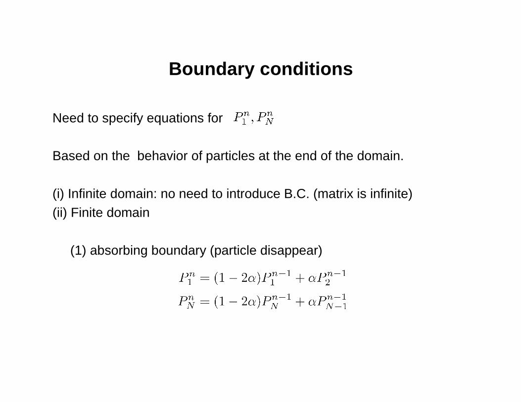
Boundary conditions
Need to specify equations for
Based on the behavior of particles at the end of the domain.
(i) Infinite domain: no need to introduce B.C. (matrix is infinite)(ii) Finite domain
(1) absorbing boundary (particle disappear)

cont..
Matrix A:

B.C. (cont.)
(2) reflecting boundary

B.C. cont.
(3) periodic B.C.
First and last rows in A change

Evolution
Where will a particle be at time n, if at time n=0 it was at position j=0?We will answer this it in two ways:
simulation using particles here we have to modify our MATLAB code randWalk1D.m to treat the different boundaries.
using the master equationhere we will use sparse matrices in MATLAB for efficient calculation. Essentially we need to apply A to the initial data n times.
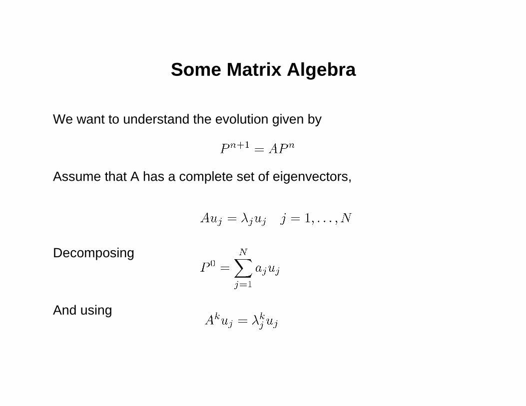
Some Matrix Algebra
We want to understand the evolution given by
Assume that A has a complete set of eigenvectors,
Decomposing
And using
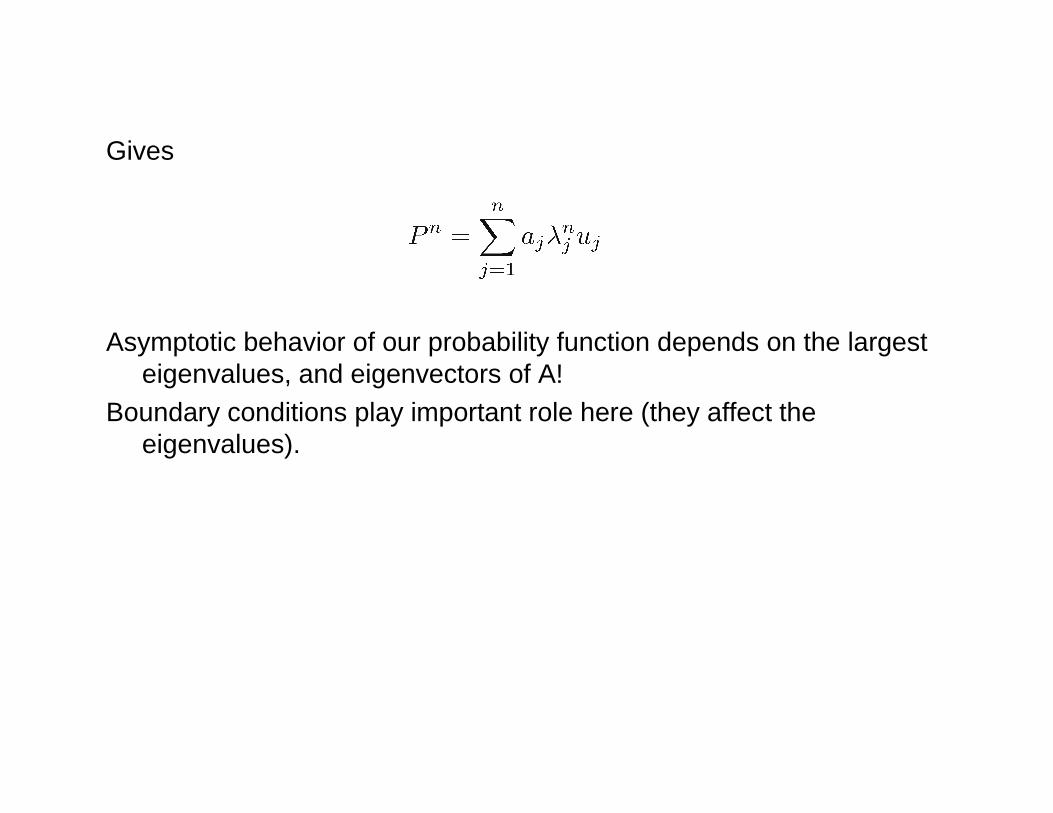
Gives
Asymptotic behavior of our probability function depends on the largest eigenvalues, and eigenvectors of A!
Boundary conditions play important role here (they affect the eigenvalues).
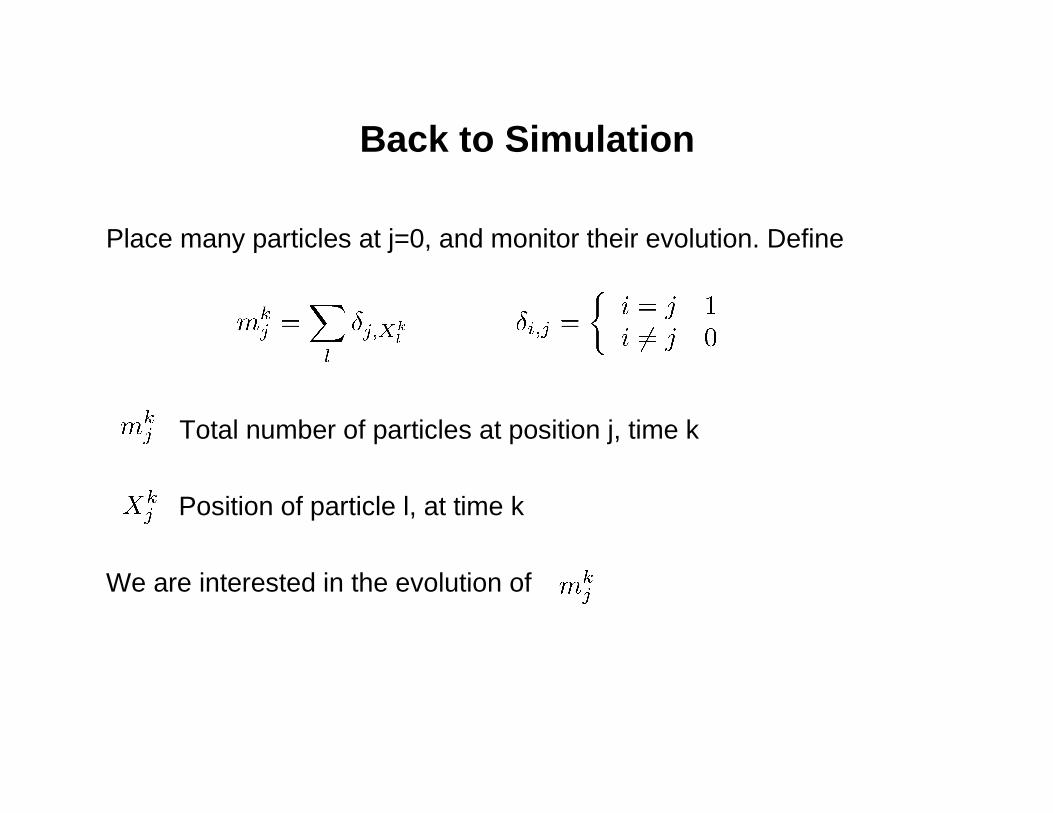
Back to Simulation
Place many particles at j=0, and monitor their evolution. Define
Total number of particles at position j, time k
Position of particle l, at time k
We are interested in the evolution of
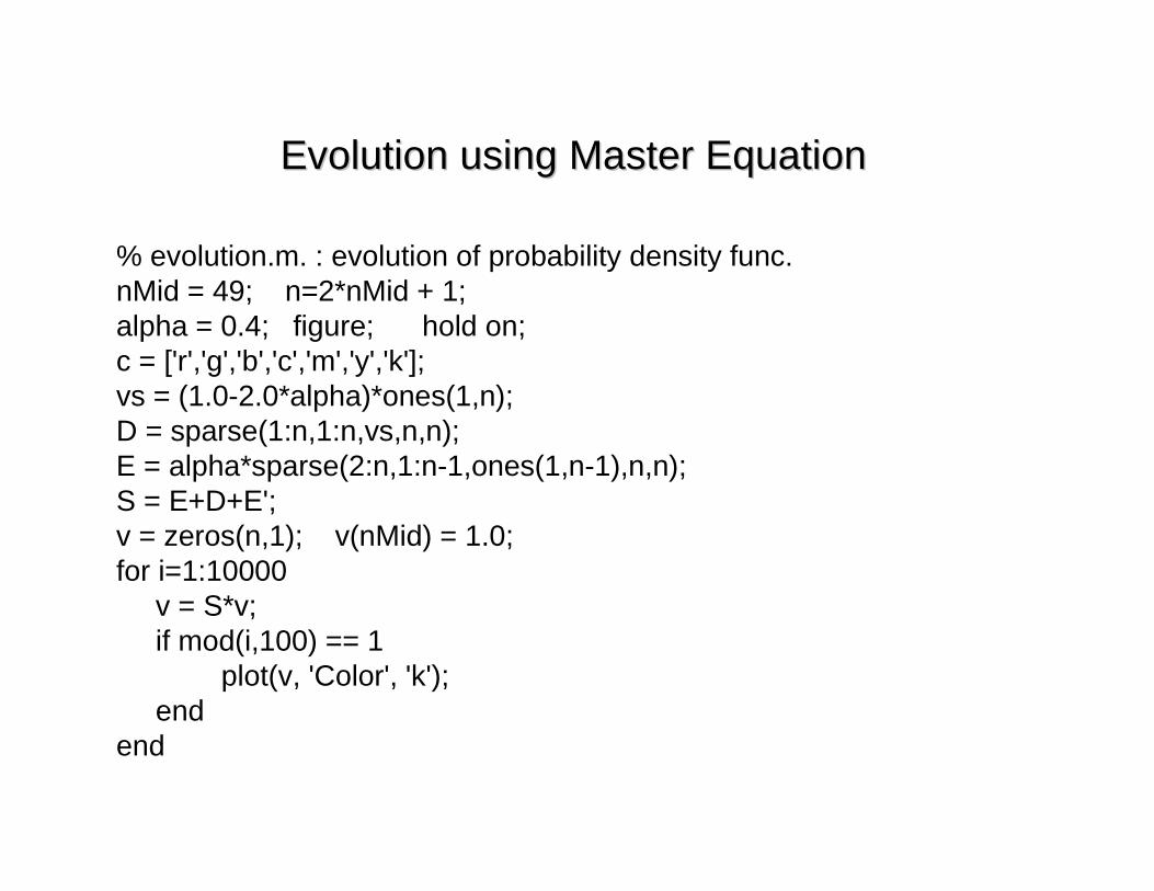
% evolution.m. : evolution of probability density func.nMid = 49; n=2*nMid + 1;alpha = 0.4; figure; hold on;c = ['r','g','b','c','m','y','k'];vs = (1.0-2.0*alpha)*ones(1,n);D = sparse(1:n,1:n,vs,n,n);E = alpha*sparse(2:n,1:n-1,ones(1,n-1),n,n);S = E+D+E';v = zeros(n,1); v(nMid) = 1.0;for i=1:10000
v = S*v;if mod(i,100) == 1
plot(v, 'Color', 'k');end
end
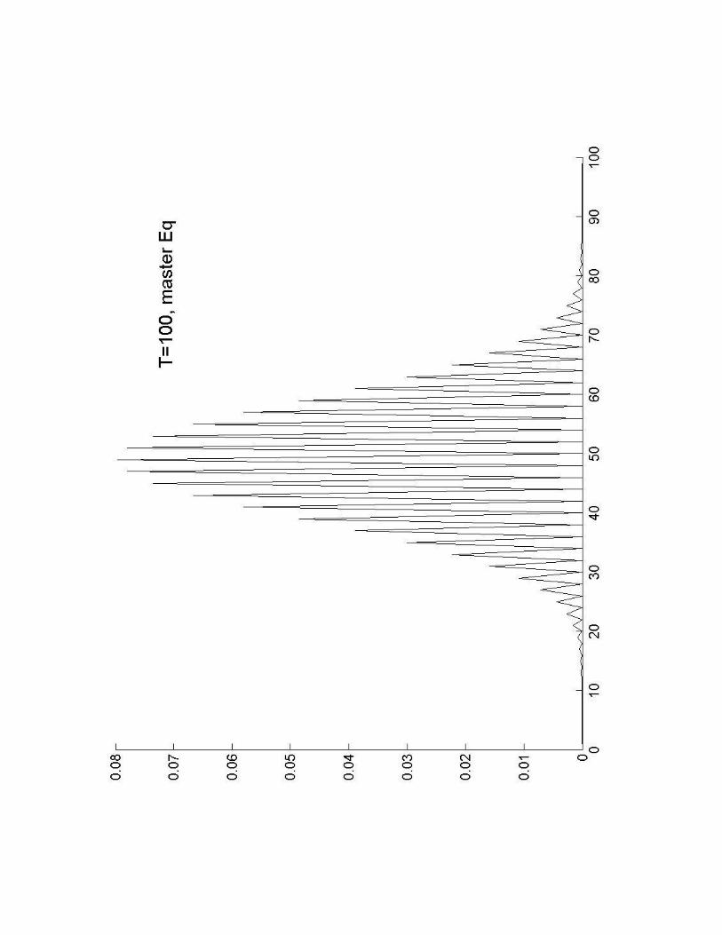
Evolution using Master EquationEvolution using Master Equation

Questions
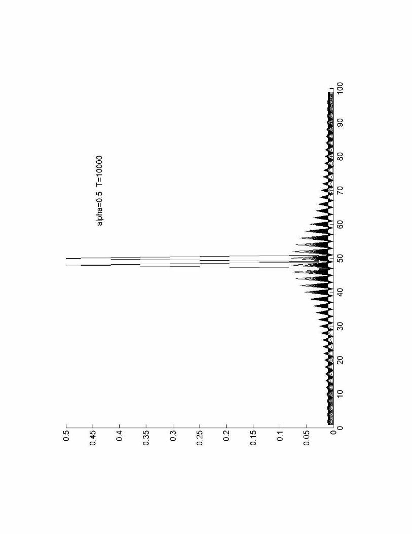
The computation shows the evolution of the probability density function, starting from a configuration where all particles are at the origin.
1. Where do the oscillation come from? 2. Can we predict the appearance of such oscillations? 3. What is the effect of different BC?
absorbing BC reflecting BC
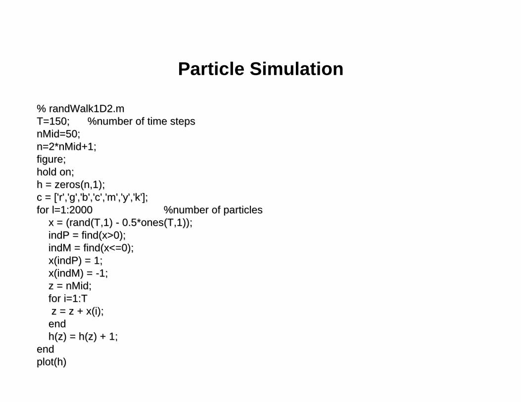
Particle Simulation
% randWalk1D2.m% randWalk1D2.mT=150; %number of time stepsT=150; %number of time stepsnMidnMid=50;=50;n=2*nMid+1;n=2*nMid+1;figure;figure;hold on;hold on;h = zeros(n,1);h = zeros(n,1);c = ['c = ['r','g','b','c','m','y','kr','g','b','c','m','y','k'];'];for l=1:2000 %number of particles for l=1:2000 %number of particles
x = (rand(T,1) x = (rand(T,1) -- 0.5*ones(T,1));0.5*ones(T,1));indPindP = = find(xfind(x>0);>0);indMindM = = find(xfind(x<=0);<=0);x(indPx(indP) = 1;) = 1;x(indMx(indM) = ) = --1;1;z = z = nMidnMid;;for i=1:Tfor i=1:Tz = z + z = z + x(ix(i););
endendh(zh(z) = ) = h(zh(z) + 1;) + 1;
endendplot(hplot(h))

Probability to Capture
Suppose that we start a random walk at the origin. What is the probability of reaching a target at x=b, by a prescribed time T?Assume also that a particle that reach x=b does not move anymore.
Using a particle simulation: start with many particle at the origin and simulate until time T. Check the fraction of particles that reached b.
Sounds easy
Can we do it using the master Equation? We need to express the fact that a particle that reaches the target disappears.

Time to Capture
Suppose that we start a random walk at the origin. What is the mean time to reach a target at x=b?
Top Related