


Languages
Pages
Legal


Use of Probabilistic Statistical Techniques in AERMOD
Modeling Evaluations
A&WMA’s 108th Annual Conference & Exhibition, Raleigh, NC, 2015
Paper #207
Sergio A. Guerra
CPP, Inc., 2400 Midpoint Drive, Suite 190, Fort Collins, CO 80525
Jesse Thé
Lakes Environmental, 60 Bathurst Drive, Unit 6, Waterloo, Ontario N2V 2A9, Canada
ABSTRACT
The advent of the short term National Ambient Air Quality Standards (NAAQS) prompted
modelers to reassess the common practices in dispersion modeling analyses. The probabilistic
nature of the new short term standards also opens the door to alternative modeling techniques
that are based on probability. One of these is the Monte Carlo technique that can be used to
account for emission variability in permit modeling.
Currently, it is assumed that a given emission unit is in operation at its maximum capacity every
hour of the year. This assumption may be appropriate for facilities that operate at full capacity
most of the time. However, in most cases, emission units operate at variable loads that produce
variable emissions. Thus, assuming constant maximum emissions is overly conservative for
facilities such as power plants that are not in operation all the time and which exhibit high
concentrations during very short periods of time.
Another element of conservatism in NAAQS demonstrations relates to combining predicted
concentrations from the AMS/EPA Regulatory Model (AERMOD) with observed (monitored)
background concentrations. Normally, some of the highest monitored observations are added to
the AERMOD results yielding a very conservative combined concentration.
A case study is presented to evaluate the use of alternative probabilistic methods to complement
the shortcomings of current dispersion modeling practices. This case study includes the use of
the Monte Carlo technique and the use of a reasonable background concentration to combine
with the AERMOD predicted concentrations. The use of these methods is in harmony with the

probabilistic nature of the NAAQS and can help demonstrate compliance through dispersion
modeling analyses, while still being protective of the NAAQS.
INTRODUCTION
Annual ambient standards have historically been addressed with deterministic methods. Under
these standards, the highest predicted concentration is compared to a set threshold. However,
this paradigm has changed with short term probabilistic NAAQS. Instead of comparing the
maximum value to a given threshold, with probabilistic standards we compare a percentile value
from the predicted concentrations to a specific threshold. For example, for the 1-hour SO2
NAAQS, the high-fourth-high (H4H) predicted concentration is compared to the 1-hour NAAQS
of 196 g/m3. That is the case because the distribution of maximum hourly values each day is
equal to 365 values (one per day) and the 99th
percentile value from such a distribution is the
3.6th
highest value which rounds to 4th
highest value also referred to as the high-fourth-high
(H4H). The aim of probabilistic standards is to reduce the likelihood of concentrations
exceeding a threshold. This means that for a modeling evaluation with a H4H concentration at
the level of the 1-hour SO2 NAAQS, the likelihood of exceeding 196 g/m3 is less than 1% (1.0-
0.99). Thus, probabilistic standards provide a stringent level of protection based on the
likelihood of complying with the NAAQS. The switch from deterministic to probabilistic
standards allows for alternative modeling techniques that are based on probability.
Whereas the use of probability in modeling demonstrations may seem foreign in dispersion
modeling, probability has been used for a long time to evaluate AERMOD’s performance.
Additionally, EPA allows the use of probabilistic methods such as the Monte Carlo approach in
other fields including health risk assessments. More recently EPA used this method in the
modeling guidance for 1-hour SO2 non-attainment designations. With this in mind, the use of
the Monte Carlo statistical technique for permitting dispersion modeling evaluations should also
be allowed. Justification for the use of a reasonable background concentration to combine with
the AERMOD predicted concentrations is included in this analysis. The use of these two
methods is in line with the probabilistic nature of the short term NAAQS and can help
demonstrate compliance through dispersion modeling analyses while still being protective of the
NAAQS.

AERMOD’s Probabilistic Performance Evaluations
The American Meteorological Society/Environmental Protection Agency Regulatory Model
(AERMOD) was rigorously evaluated before it was incorporated by EPA as the preferred near-
field dispersion model for regulatory applications in the Guideline on Air Quality Models
(Appendix W to 40 CFR Part 51). These evaluations involved comparisons between predicted
(modeled) and observed (monitored) concentrations from 17 studies. The databases from these
studies are available in EPA’s Support Center for Regulatory Atmospheric Modeling.1
EPA employed Quantile-Quantile (Q-Q) plots to evaluate AERMOD’s performance for
predicting compliance with air quality regulations.2 These plots compare predicted and observed
concentrations from the databases available. While these values are originally paired in time and
space, the spatial and temporal alignment is lost in the ranking process. That is the case because
Q-Q plots compare the sorted list of predicted concentrations with the sorted list of observed
concentrations.
A more rigorous test would involve comparing predicted and observed concentrations on a
scatterplot with data paired in time and space. However, AERMOD has been shown to have
poor correlation on a spatial and temporal basis. 3-7
Nonetheless, EPA uses Q-Q plots to evaluate
model performance because the distribution of maximum and minimum values tends to follow a
similar pattern between predicted and observed concentrations. This means that, whereas the
model is not able to predict the exact location and the exact time of a maximum concentration,
the model is able to provide with good accuracy the likelihood of experiencing a maximum
occurrence within a given time period (5 years or 1 year if using on-site meteorological data).
Section 9.1.2 Studies of Model Accuracy from Appendix W summarizes this as follows:
Models are reasonably reliable in estimating the magnitude of highest concentrations
occurring sometime, somewhere within an area.
This means that we cannot assume that the highest concentration obtained with AERMOD will
be located at the exact receptor and at the exact time identified by AERMOD. On the other
hand, measured concentration distribution is similar to the one predicted in AERMOD. Thus, it
should be recognized that the results from AERMOD are probabilistic in nature. With this in
mind, the EPA has established probabilistic standards (e.g., 98th
percentile) for the new NAAQS
(e.g., 1-hour NO2, 24-hour PM2.5).
Regardless of the lack of temporal and spatial correlation between predicted and observed
concentrations, AERMOD is able to predict the likelihood of exceedances happening in a given
receptor grid over a given period of time (e.g., 5 years).
Monte Carlo Statistical Technique
The Monte Carlo technique is the probabilistic technique proposed to address some of
AERMOD’s conservative assumptions is. Numerous fields of science and industry widely use
and accept this statistical procedure. The Manhattan Project scientists developed this statistical
approach in the 1940’s to estimate neutron multiplication rates to predict the explosive behavior
of neutron chain reactions in fission weapons.8 The EPA already has a long standing policy in
place to allow Monte Carlo analyses in risk assessments.9,10,11
More recently, EPA pioneered the
use of the Monte Carlo technique in its evaluation included in the Guidance for 1-hr SO2
Nonattainment Area SIP Submissions.12
In Appendix B of this guidance EPA introduces the
concept of using of a longer term average emission limit to be comparable in stringency with the
1-hour average limit. EPA performed a Monte Carlo analysis to justify this approach by using
100 randomly reassigned emission data and single years of emissions data to characterize
emission variability over a 5‐year period of meteorology. This evaluation concluded that if
periods of hourly emissions above the critical emission value were rare occurrences at a source,
these periods would be unlikely to have a significant impact on air quality, insofar as they would
be very unlikely to occur repeatedly at the times when the meteorology is conducive for high
ambient concentrations. In other words, the method outlined by EPA allows for sporadic
emission spikes that would not be allowed with a 1‐hr limit, but compensates by adopting a
lower average emission rate over a longer averaging time such that the likelihood (probability) of
having high emissions and poor dispersion characteristics is minimized.
Emission Variability Processor (EMVAP)
The Electric Power Research Institute (EPRI) commissioned the EMVAP technique a tool to
incorporate the transient and variable operations of emission units in a modeling analysis.

EMVAP employs the Monte Carlo statistical technique, which as discussed earlier, has been
allowed by EPA for risk assessments and 1-hr SO2 non-attainment modeling. EMVAP creates a
frequency distribution from given emission sources by assigning emission rates from a pool of
emissions (usually from CEMS data) at random over numerous iterations. The resulting
distribution yields a more realistic approximation of actual modeled impacts. EMVAP has been
evaluated extensively13-15
for dispersion modeling applications.
The assumption of constant emissions is not appropriate for emission units that operate
infrequently, at variable loads, or that have infrequent high emissions. For these cases the
EMVAP probabilistic approach is more suitable to accurately characterize the effect from these
emission profiles.
Combining Background Concentrations in NAAQS Modeling Evaluations
Background concentrations are commonly obtained from representative ambient monitors.
However, most of these monitors are sited to capture maximum impacts in a given area16
. Thus,
finding ambient monitors that are truly representative of background levels of ambient air is
challenging. Additionally, it is a common practice to pair predicted concentration from
AERMOD with maximum recorded observation from the ambient monitor. EPA made some
concessions on this practice17,18
and now allows a Tier 2 approach where a reduced subset of
monitored observations are grouped by seasons and combined with predicted AERMOD
concentrations on a seasonal basis. This approach assumes that AERMOD concentrations are
sufficiently correlated with monitored concentrations on a temporal basis (hour by hour).
However, as discussed previously, AERMOD results are evaluated irrespective of time and space
(i.e., with Q-Q plots) since model performance significantly decreases when analyzed on a
temporal basis3-7
. Thus, temporal pairing of modeled and monitored concentrations is
unjustified.
Screening of Background Concentrations
When meteorological data is available, it may be possible to exclude the monitored observations
that occur when the monitor is being impacted from these sources.
Nicholson19
described a screening technique to obtain a representative background concentration
by analyzing hourly PM2.5 monitored data from the Santa Fe, New Mexico airport monitoring
site. Nicholson screened out monitoring observations from unusual events and occurrences
when the monitor was downwind of a major emission source. After screening out exceptional
events, the resulting 98th
percentile concentration was 6 g/m3 compared to 18 g/m
3 obtained
from the unscreened data set. Nicholson cautioned against the use of background concentrations
based upon extreme values since these are not representative of the background in a dispersion
modeling domain.
The EPA defines exceptional events as unusual or naturally occurring events that can affect air
quality but are not reasonably controllable.20
However, the flagging of exceptional events is only
performed by State agencies when there are attainment issues. Therefore, the data collected from
these monitors contains observations that overpredict background concentrations.
The challenge in determining a representative background value is how to screen out the
observations from times when the monitor is downwind from a given emission source to avoid
double counting emissions. However, it is possible to filter out the effects from explicitly
modeled sources and exceptional events (e.g., forest fires, sand storms, etc.) by analyzing the
distribution of monitored observations as proposed below.
Combining Modeled Results and Background Concentrations
The 1-hour SO2 NAAQS was promulgated as the 99th
percentile of maximum daily
concentrations. Thus, the probability of this standard is 1.00 - 0.99 = 0.01. This is equivalent to
1 exceedance every 100 days (1/100 = 0.01). When we extrapolate this ratio to the number of
days in a year (365) we get 3.6 exceedances in a year which is rounded up to the 4th highest
value in a year. Thus, the form of the standard is the high-fourth-high (H4H) value from the daily
maximum 1-hour values across a year. However, by assuming that the 99th
percentile modeled
concentration is combined with the 99th
percentile background concentration, the probability
equals 0.0001 or (0.01) * (0.01). This is equivalent to the 99.99th
percentile or one exceedance
every 10,000 days (1/10,000 = .0001), representing one exceedance every 27 years. The
probabilistic inappropriateness of such an approach has been described previously.6

Furthermore, this degree of conservatism is well beyond the level necessary to protect the
NAAQS.
A more realistic approach in NAAQS dispersion modeling analyses is to combine AERMOD’s
concentrations with the 50th
percentile background concentration.21
This approach conserves the
use of the modeled 99th
percentile value from AERMOD and allows for a more representative
background level by selecting the median instead of the tail of the distribution. Additionally, this
approach will still be protective of the NAAQS because it results in a marginal probability of
0.005 or (0.01) * (0 .50). This is equivalent to the 99.5th
percentile combined concentration
which is more conservative than the 99th
percentile standard. Therefore, this method is
statistically sound and provides a reasonable level of conservatism that ensures the protection of
the NAAQS.
EXPERIMENTAL METHODS
The current study evaluates the predicted concentrations based on three cases:
1. Using AERMOD by assuming a constant maximum emission rate (current modeling
practice)
2. Using AERMOD by assuming a variable emission rate
3. Using EMVAP to account for emission variability
The modeling evaluation is based on one year of emission data from a power plant. These data
were scaled up for the following example. In other words, its emission profile is the same but the
magnitude has been adjusted. A graphical representation of the emission profile for this
hypothetical power plant is shown in Figure 1.
The assumptions and the modeling parameters for these cases are summarized in Table 1.
AERMOD version 14134 was used with meteorological data processed for one year with
AERMET version 12345. The receptor grid is comprised of 1,080 polar receptors extending
7,500 meters from the source.

Table 1. Three cases used to model the power plant.
Input parameter Case 1 Case 2 Case 3
Description of
Dispersion
Modeling
Current
Modeling
Practices
AERMOD with
hourly emission
EMVAP
(500 iterations)
SO2 Emission rate
(g/s) 478.7
Actual emission
rates from
CEMS data
Bin1: 478.7
(5.0% time)
Bin 2: 228.7
(95% time)
Stack height (m) 122
Exit temperature
(degrees K) 416
Diameter (m) 5.2
Exit velocity (m/s) 23
Figure 1. Emission distribution by percentiles.
RESULTS AND DISCUSSION
The results for the three cases described are summarized below (Table 2). Case 1 produced the
highest concentrations and exceeded the NAAQS. This is not surprising given that Case 1
assumes continuous emissions at the highest emission rate. Case 2 resulted in the lowest
concentration; about 40% of the NAAQS. However, this is presented for comparison purposes
only and should be viewed with caution because AERMOD has negligible correlation with

monitored concentrations on a temporal basis. Case 3 was calculated from 500 iterations in
EMVAP and resulted in a 99th
percentile concentration that is 92% of the NAAQS. These results
do not include impacts from neighboring sources and background concentrations.
Table 2. Results of 1-hour SO2 concentrations for the three cases.
Case 1
(µg/m3)
Case 2
(µg/m3)
Case 3
(µg/m3)
Description of
Dispersion
Modeling
Current
Modeling
Practices
AERMOD
with hourly
emission
EMVAP
(500 iterations)
H4H 229.9 78.6 179.3
Percent of
NAAQS 117% 40% 92%
Background Concentrations
According to the Annual Air Monitoring Network Plan for Minnesota,22
the MPCA monitors
SO2 at six sites. The 2011-2013 average 99th
percentile 1-hr SO2 concentrations range from 5.2
µg/m3
to 89.0 µg/m3. Out of these, the Saint Paul Park 436 monitor was selected since it records
the second highest three year average concentration (26.2 µg/m3). The Saint Paul Park 436
monitor is located about 9 miles southeast of downtown St. Paul, Minnesota. The location is east
of the Mississippi River and is surrounded by industrial land including an oil refinery (Figure 2).

Figure 2. St. Paul Park 436 ambient monitor location.
Hourly ambient air monitoring data was obtained from EPA’s Airdata web site23
for the Saint
Paul Park 436 monitor for the years 2011 through 2013. The monitoring data is recorded in parts
per billion (ppb) and contained only the maximum hourly observations by day. Therefore, there
were 365 maximum hourly values for 2011 and 2013, and 366 maximum values for 2012 (leap
year). These values were analyzed to find a representative 1-hour background concentration.
The observations were analyzed in the histogram below (Figure 3). The histogram exhibits a
long right tail due to few very high observations. However, the most frequent observation
recorded was 2.6 g/m3 (1 ppb) which occurred 40 percent of the time. Table 3 presents the
distribution of concentrations at different percentiles. The Annual Air Monitoring Network Plan
for Minnesota shows the three-year average of the annual 99th
percentile daily maximum 1-hour
SO2 concentrations to be 10 ppb (about 26.2 g/m3), which is one order of magnitude higher
than the most frequent observation (1 ppb). Thus, from the histogram below, it is overly
conservative to assume that a 10 ppb concentration is present every hour of the year.
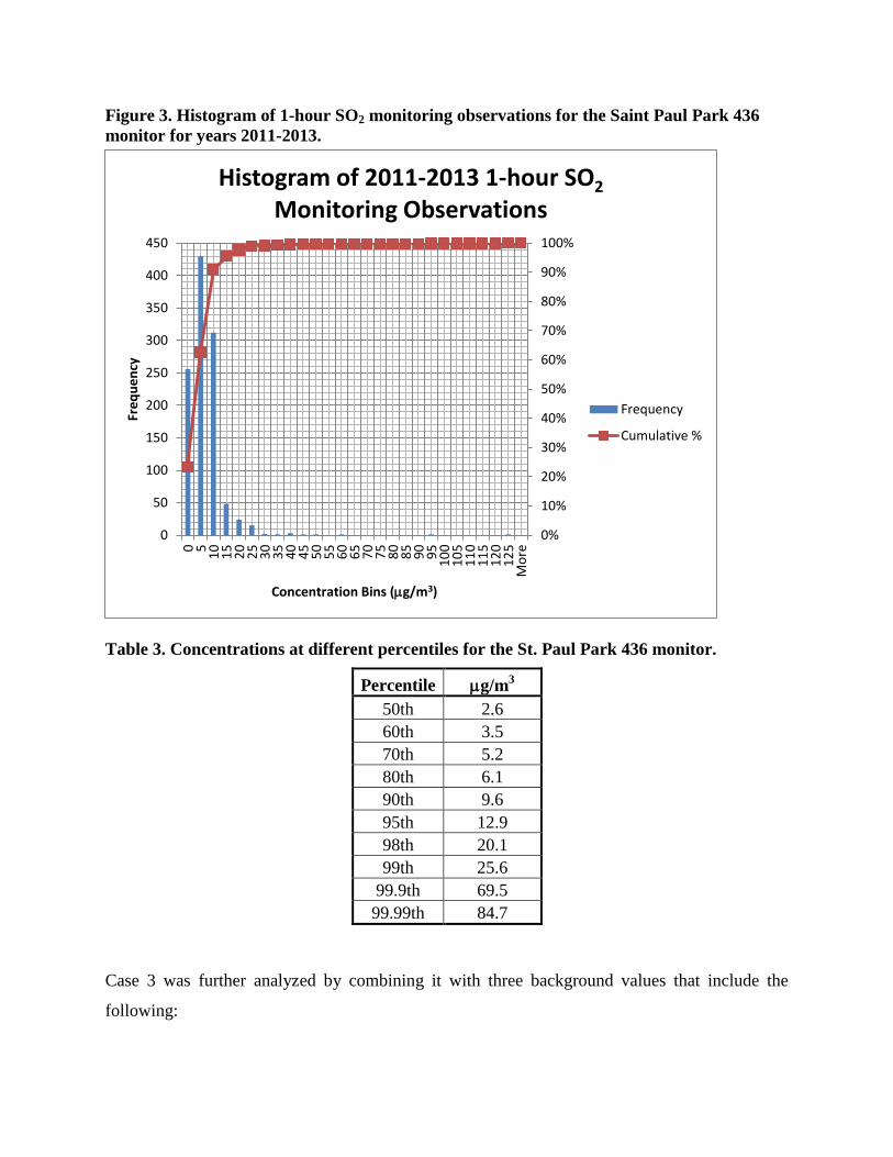
Figure 3. Histogram of 1-hour SO2 monitoring observations for the Saint Paul Park 436
monitor for years 2011-2013.
Table 3. Concentrations at different percentiles for the St. Paul Park 436 monitor.
Percentile g/m3
50th 2.6
60th 3.5
70th 5.2
80th 6.1
90th 9.6
95th 12.9
98th 20.1
99th 25.6
99.9th 69.5
99.99th 84.7
Case 3 was further analyzed by combining it with three background values that include the
following:
0%
10%
20%
30%
40%
50%
60%
70%
80%
90%
100%
0
50
100
150
200
250
300
350
400
450
0 51
01
52
02
53
03
54
04
55
05
56
06
57
07
58
08
59
09
51
00
10
51
10
11
51
20
12
5M
ore
Fre
qu
en
cy
Concentration Bins (g/m3)
Histogram of 2011-2013 1-hour SO2 Monitoring Observations
Frequency
Cumulative %

1. Bkg 1: Three year average of maximum daily 1-hour SO2 observations.
2. Bkg 2: Three year average of the 99th
percentile daily maximum 1-hour
SO2 observations.
3. Bkg 3: Three year average of the 50th
percentile daily maximum 1-hour
SO2 observations.
Bkg 1 is representative of the value initially recommended by EPA (Tier 1). In more recent
guidance14
EPA allowed the use of the three year average 99th
percentile daily maximum
observations for the 1-hour SO2 concentrations. However, as discussed previously, assuming
that two exceptional events occur at the same time is excessively conservative. Thus, the use of
the 50th
percentile is a more reasonable assumption that was evaluated as Bkg 3. The results in
Table 4 show that Bkg 1 and Bkg 2 exceed the 1-hour SO2 NAAQS. However, by assuming a
more reasonable background concentration (i.e., Bkg 3), the 1-hour SO2 NAAQS are met in this
hypothetical analysis.
Table 4. Case 3 with three different background values.
Case 3 with Bkg 1
(µg/m3)
Case 3 with Bkg 2
(µg/m3)
Case 3 with Bkg 3
(µg/m3)
H4H 179.3 179.3 179.3
Background 86.4 25.6 2.6
Total 265.7 204.9 181.9
Percent of NAAQS 135.6% 104.5% 92.8%
SUMMARY
The newly promulgated NAAQS herald a new era of dispersion modeling with its probabilistic
nature. The use of probabilistic techniques is consistent with the evaluations performed to
validate the use of AERMOD. Combining the use of AERMOD with the Monte Carlo technique
is appropriate when used to account for emission variability inherent in many emission sources.
Furthermore, this technique is already allowed by EPA for risk assessments and more recently
for modeling of non-attainment modeling of 1-hour SO2. Consequently, the use of EMVAP to
account for the emission variability of emission units allows for more reasonable results in
dispersion modeling analyses. EMVAP is especially useful in cases where the emission units
evaluated have an infrequent use or variable load. The use of this modeling technique can result

in more reasonable predicted concentrations that are still protective of the NAAQS.
Furthermore, as shown in this study, combining the 50th
percentile monitored concentration with
the 99th
percentile predicted concentration (1-hr SO2) should be considered in regulatory
applications. In summary, more realistic results can be obtained from AERMOD by addressing
emission variability with a Monte Carlo approach and by pairing predicted concentrations with
the median observed values.
REFERENCES
1. U.S. EPA SCRAM web site: http://www.epa.gov/ttn/scram/dispersion_prefrec.htm
(Accessed February 2015)
2. AERMOD: Latest Features and Evaluation Results. EPA-454/R-03-003, June 2003.
3. Bowne, N.E. and R.J. Londergan, 1983. Overview, Results, and Conclusions for the EPRI
Plume Model Validation and Development Project: Plains Site. EPRI EA–3074. Electric
Power Research Institute, Palo Alto, CA.
4. Moore, G.E., T.E. Stoeckenius and D.A. Stewart, 1982. A Survey of Statistical Measures of
Model Performance and Accuracy for Several Air Quality Models. Publication No. EPA–
450/4–83–001. Office of Air Quality Planning & Standards, Research Triangle Park, NC.
(NTIS No. PB 83–260810).
5. EPRI, 1988. Urban Power Plant Plume Studies. EPRI EA-5468. Electric Power Research
Institute, Palo Alto, CA.
6. Murray, D. R.; Newman, M. B. (2014). “Probability Analyses of Combining Background
Concentrations with Model Predicted Concentrations.” Journal of Air & Waste Management
Association.
7. Frost, K. D. (2014). “AERMOD Performance Evaluation for three Coal-fired Electrical
generating Units in Southwest Indiana.” Journal of Air & Waste Management Association.
8. Eckhardt, R. “Stan Ulam, John von Neumann, and the Monte Carlo Method.” Los Alamos
Science, Special Issue, 1987.
Available from: http://library.lanl.gov/cgi-bin/getfile?15-13.pdf
9. U.S. EPA, “Policy for use of Probabilistic Analysis in Risk Assessment”, may 15, 1997.
10. U.S. EPA, “Guiding Principles for Monte Carlo Analysis”, EPA/630/R-97/001, March, 1997.
11. U.S. EPA, “Draft Guidance for Submission of Probabilistic Exposure Assessments to the
Office of Pesticide Programs’ Health Effects Division”, February 6, 1998.
12. U.S. EPA (2014), “Guidance for 1-hr SO2 Nonattainment Area SIP Submissions”, Stephen
Page guidance dated April 23, 2014. Office of Air Quality Planning and Standards, Research
Triangle Park, NC.
13. Paine, R.; Hamel, R.; Heinold, D.; Knipping, E.; Kumar, N. “Early Experiences with
EMVAP Implementation and Testing.” Paper 12827. In Proceedings of the Air & Waste

Management Association’s Annual Conference and Exhibition in Chicago, IL. June 25-28,
2013.
14. Kumar, N. “Development, Testing and Evaluation of EMVAP and SCICHEM.“ Presented at
the EPA Regional/State/Local Modelers Workshop in Dallas, TX. April 23, 2013.
15. Paine, R.; Hamel, R.; Kaplan, M.; Heinold, D.; Knipping, E.; Kumar, N. Progress Report:
Further EMVAP Development, Testing, and Evaluation.” Presented at the Air & Waste
Management Association’s Specialty Conference in Raleigh, NC. March 19-21, 2013.
16. U.S. EPA. (1987). “Ambient Monitoring Guidelines for Prevention of Significant
Deterioration (PSD).” EPA‐450/4‐87‐007, Research Triangle Park, NC.
17. U.S. EPA. (2011). “Additional Clarification Regarding Application of Appendix W
Modeling Guidance for the 1-hour NO2 NAAQS.” Tyler Fox memorandum dated March 1,
2011.
18. U.S. EPA. (2011). “Guidance for PM2.5 Permit Modeling.” Stephen Page guidance dated
May 20, 2014. EPA-454/B-14-001, Research Triangle Park, NC.
19. Nicholson, B. R., (2013). “Background Concentration and Methods to Establish Background
Concentrations in Modeling.” Presented at the Guideline on Air Quality Models: The Path
Forward. Raleigh, NC.
20. U.S. EPA (2007) "Treatment of Data Influenced by Exceptional Events; Final Rule" (72 FR
13560) pursuant to the 2005 amendment of CAA Section 319.
21. Guerra, S.A.; Olsen, S.; Anderson, J., (2014). ” Evaluation of the SO2 and NOx Offset Ratio
Method to Account for Secondary PM2.5 Formation.” Journal of Air & Waste Management
Association.
22. Gavin, K.; McMahon, C., (2014). ”Annual Air Monitoring Network Plan for Minnesota”,
Minnesota Pollution Control Agency, Saint Paul, MN.
23. U.S. EPA Airdata web site: http://www.epa.gov/airquality/airdata/
(Accessed September 2014)
KEYWORDS
Monte Carlo, AERMOD, background concentrations, EMVAP
Top Related