


Languages
Pages
Legal


UNIVERSITY OF OKLAHOMA
GRADUATE COLLEGE
INTERACTIVE WEB-BASED TOOL FOR CREATING 3-D ENGINEERING
SIMULATIONS USING FLASH
A THESIS
SUBMITTED TO THE GRADUATE FACULTY
in partial fulfillment of the requirements for the
Degree of
MASTER OF SCIENCE
By
SUYOG LOKHANDE
Norman, Oklahoma
2010

INTERACTIVE WEB-BASED TOOL FOR CREATING 3-D ENGINEERING
SIMULATIONS USING FLASH
A THESIS APPROVED FOR THE
SCHOOL OF AEROSPACE AND MECHANICAL ENGINEERING
BY
Dr. Kurt Gramoll, Chair
Dr. Harold Stalford
Dr. Zahed Siddique

© Copyright by SUYOG LOKHANDE 2010
All Rights Reserved.

iv
Acknowledgements
It was a great journey of doing Masters at University of Oklahoma. I would like to
express my utmost gratitude to Prof. Gramoll for his guidance and all the support he
provided during this master‟s thesis. I am also grateful for Prof. Stalford and Prof.
Siddique for providing the valuable guidance, suggestion, and comments throughout the
thesis.
I also like to convey my sincere thanks to my co-workers in Engineering Media
Lab (EML) for offering valuable suggestions and for making my Masters as a pleasant
journey.
It was almost impossible for me to finish my graduation without the valuable
support of my cousin Dr. Mangesh Edke and my friends Dr. Alok Tongaonkar, Lalit
Deshpande, Aashish Wadke. I also wish to extend my heartfelt gratitude to my friends,
Parag Gujar, Gauri Gujar, Arindam Basu, and Indrani Basu for making my stay
comfortable and enjoyable at US.
Above all, I sincerely thank my parents, Mr. Subhash Lokhande, Mrs. Sujata
Lokhande and my sisters, Shilpa and Kavita for supporting me throughout this time.
Without which, this thesis and the masters program would not have been a great success.
v
Table of Contents
List of Illustrations ............................................................................................................ vii
Abstract .............................................................................................................................. ix
Chapter 1: Introduction ....................................................................................................... 1
1.1 Background .......................................................................................................... 1
1.2 Implementation of 3-D ......................................................................................... 3
1.3 Research Objective ............................................................................................... 7
1.4 Thesis Outline ...................................................................................................... 9
Chapter 2: Literature Review ............................................................................................ 10
Chapter 3: Parametric Modeling ....................................................................................... 13
3.1 Curves in Parametric Modeling .......................................................................... 14
3.2 Curve Restrictions Imposed ............................................................................... 17
Chapter 4: 3-D Modeling Using Adobe Flash .................................................................. 19
4.1 Sandy Pipeline Running Behind ........................................................................ 20
4.2 Procedure to Display 3-D Objects ...................................................................... 21
4.3 Creation of 3-D Cone ......................................................................................... 22
Chapter 5: Detection of a 3-D Object on a Surface and Finding the Slope of a Surface .. 24
5.1 Importance of a Triangular Surface for Creating a 3-D Surface ........................ 24
5.2 Sphere Inside the Triangle .................................................................................. 25
Area Technique.......................................................................................................... 25
Same side Technique ................................................................................................. 26
Barycentric Technique ............................................................................................... 27
5.3 Finding the Slope of 3-D Surface ....................................................................... 31
Chapter 6: Motion Detection between a 3-D Object and a 3-D Surface .......................... 33
6.1 Find the 3-D Surface and Move the 3-D Sphere Approach ............................... 33
6.2 Find the Adjacent Triangles of the Parent Triangle Approach .......................... 34
6.3 Projecting the Sphere inside the Triangle Approach .......................................... 36
6.4 Restricting the Sphere inside a Triangle Approach ............................................ 39
Chapter 7: Testing and Performance ................................................................................. 41
7.1 Zero Initial Velocity in X and Y Direction to the Sphere Test .......................... 41
7.2 Moving the Sphere across a Simple Cone .......................................................... 42

vi
7.3 Moving the Sphere across the Cone with Initial Velocity in X and Y Direction45
7.4 Moving the Sphere across the Cone having „U‟ section and with Initial
Velocity in X Direction ......................................................................................... 46
Chapter 8: Conclusion....................................................................................................... 49
8.1 Summary ............................................................................................................ 49
8.2 Recommendations and Future Scopes................................................................ 50
References ......................................................................................................................... 51
Appendices .................................................................................................................... 53
Appendix 1: ActionScript code for creating a Bezier Curve ........................................ 53
Appendix 2: ActionScript code for creating 3-D Cone ................................................. 54
Appendix 3: ActionScript code for the 3-D Sphere Movement on a 3-D Surface ........ 58
vii
List of Illustrations
Figure 1: Example showing use of electronic media in teaching engineering concepts
from eCourses.ou.edu .......................................................................................... 3
Figure 2: Example showing use of Director for displaying 3-D objects ............................ 5
Figure 3: Example showing use of Java3-D for displaying 3-D objects over the Internet . 6
Figure 4: Different views of a 3-D cone created in Adobe Flash ....................................... 8
Figure 5: Cubic Bezier curve (light blue color) with four control points ......................... 15
Figure 6: Twisted Bezier curve (light blue color) with four control points ...................... 16
Figure 7: Restriction imposed for creating Bezier curve .................................................. 17
Figure 8: Different Bezier curves obtained after restrictions imposed on control points . 18
Figure 9 : Cone creation by rotating a Bezier curve ......................................................... 23
Figure 10: Area technique to determine whether point is inside the triangle ................... 25
Figure 11: Same side technique to determine whether point is inside the triangle ........... 26
Figure 12: Cross product technique for determining point position ................................. 27
Figure 13: Barycentric technique - checking point position (condition - 1) ..................... 28
Figure 14: Barycentric technique - checking point position (condition - 2) ..................... 30
Figure 15: Barycentric technique - checking point position (condition - 3) ..................... 30
Figure 16: Finding the slope of a 3-D surface .................................................................. 32
Figure 17: Flowchart for finding the slope of 3-D surface and moving the 3-D sphere
approach ............................................................................................................. 34
Figure 18: Flowchart for find the adjacent triangles of the parent triangle approach ....... 35
Figure 19: Projecting a point on a plane ........................................................................... 36

viii
Figure 20: Flowchart for projecting the sphere inside the triangle ................................... 38
Figure 21: Black-hole position for a 3-D sphere .............................................................. 39
Figure 22: Flowchart for restricting the sphere inside a triangle approach ...................... 40
Figure 23: Zero initial velocity in X and Y direction to the sphere test ........................... 42
Figure 24: Straight edge cone for test case scenario ......................................................... 43
Figure 25: Moving the sphere across a straight line cone. ................................................ 44
Figure 26: Moving the sphere across the cone with initial velocity in X and Y direction 46
Figure 27: Moving the sphere across the cone having „U‟ section and with initial
velocity in X direction ....................................................................................... 47

ix
Abstract
Numerous companies and universities have adopted web-based education because
of its ability to overcome the barriers of distance, time, and various operating platforms.
One of the key challenges in delivering engineering education online is direct simulation
of 3-D engineering models through a web browser. Therefore, developing interactive 3-D
learning tools is important for enriching learning experience for engineering students as
well as facilitating communication within the engineering industry. The primary
objective of this research is to develop interactive, web-based tool for creating 3-D
technical models for engineering learning and training.
Currently, Adobe Flash CS3 (or CS4) and third party classes from Sandy3D can
be used for modeling basic 3-D shapes, such as cubes, spheres, cylinders and cones.
However, these models are developed for advertisement or gaming purposes and rarely
satisfy the needs of engineers. Also, there is no „revolve‟ function present in their models
which can be used for generating complicated mechanical shapes.
In this thesis, an interactive 3-D cone like funnel shape was created by rotating a
„Bezier curve.‟ To ensure geometric feasibility, limitations on the movement of the
control points for the „Bezier curve‟ were imposed. Mechanical assembly could not be
completed without interacting more than two models. To illustrate this functionality, a
sphere was created and placed on the top edge of the cone. The sphere slides inside the
cone using the slope of the cone as the boundary condition. The sphere‟s velocity
increases over time because of the slope of the cone.

x
Development of 3-D technical models in Adobe Flash was the main
accomplishment of this thesis. 3-D interactive technical models were created using
Adobe Flash CS3 (also referred as Flash 9), Sandy3D, and the ActionScript 3.0 language
(part of Adobe Flash). A graphical user interface was developed in Flash and the code
was tested using different cross sections of the funnel. The results agree well with the
prediction and are documented in this thesis. The code developed in this research can be
used to model similar problems involving different 3-D geometric shapes. Also, this
research explores different possible usage of this 3-D technical model generating code to
enhance better displays of 3-D engineering models on web pages.

1
Chapter 1
Introduction
1.1 Background
Due to tremendous advancement in technology, the emergence of the global
knowledge economy is placing an increasing importance on lifelong learning. Continuing
education, which is a new trend in the engineering field, can be defined as a formal
education, provided by an employer or from a traditional educational system, beyond the
bachelor‟s degree other than the master‟s and doctorial programs. Education and training
are two closely related terms but there is a slight difference between the two. Education is
a broader learning experience covering a particular field of study, whereas training
targets specific skills required to perform job activities. In the knowledge economy, this
distinction quickly breaks down. In engineering, yesterday‟s education can become
today‟s training. Lectures and laboratories are two major ways to deliver engineering
education, but they are not efficient and cannot be scaled to teach large numbers of
students. Also, they are not suitable to teach small batches where employees join an
organization at different times of the year. So, organizations establish computer-based
learning centers where employees can learn new technologies at their convenience, time,
and place (Bourne, et al. 1997).
To satisfy the increasing demand of education from corporations as well as
individuals who cannot attend a university, corporate universities have entered the
market. The main purpose of corporate universities is to design and deliver cost-effective
learning to cater to the corporate goals. These universities generally adopt the web-based

2
learning style because of the flexibility it offers in terms of distance and time. Some
corporate universities are nearly 100 percent web-based and almost all have some web-
based elements. It is estimated that almost 50 to 75 percent of corporate education is web-
based (Bourne, Harris and Mayadas 2005). Companies can also reduce their cost to
update the skills of their employees through web-based education. According to
American Society for Training and Development, the Internet-based learning will
continue to grow in the future (Tampone 2009).
To successfully implement web-based learning in engineering, the fundamental
modes in which engineering education is traditionally delivered, namely lectures and
laboratory education, must be updated. Researchers have started thinking about different
possible ways to deliver laboratory-based education in a web-based environment. The
Accreditation Board for Engineering and Technology (ABET), which accredits programs
in engineering and technology, has started working on developing this new way of
delivering engineering education. ABET also came up with the final list of learning
objectives for engineering education laboratories during the conference funded by Alfred
P. Sloan Foundation (Peterson and Feisel 2004).
The Engineering Media Lab (EML) at the University of Oklahoma has been
developing different online engineering courses which help engineering students to
understand mechanical engineering concepts. EML has developed online learning courses
called eCourses to teach basic engineering classes, such as Statics, Dynamics, Fluids,
Thermodynamics, Mathematics, Mechanics, MEMS, and Multimedia. The eCourses
website (eCourses.ou.edu) has a variety of learning resources like eBooks, homework,
quizzes, solutions, and simulations. Figure 1 shows a screen shot of the website,

3
eCourses.ou.edu (Mechanics eBook, Chapter 4), which provides ideas to use an
electronic media in teaching the mechanical engineering concepts.
Figure 1: Example showing use of electronic media in teaching
engineering concepts from eCourses.ou.edu
1.2 Implementation of 3-D
A critical difference between engineering education and other education is that it
involves laboratory work and explanation of engineering concepts that often requires 3-D
visualization, which is hard for students to imagine. Web-based engineering education
will be effective if a 3-D interactive tool is available. However, it is found that most of
the current web-based educational websites do not present 3-D objects (Sun, Stubblefield
4
and Gramoll 2000). One of the important factors for accessing a web site having 3-D
objects is the constraint on bandwidth. For a fixed bandwidth, if the size of the 3-D object
is large, it will require too much time to load and students will lose interest.
Another important challenge in engineering education is the difficulty involved in
showing interactive 3-D models over the Internet. Although, numerous Mechanical
Engineering tools like Pro/E, CATIA, and SolidWorks are available for creation of 3-D
engineering models, they are not useful for showing 3-D interactive models over the
Internet. There are two reasons behind this: (i) the file size is large, and (ii) the model
must be exported to a web-compatible file format (for example, VRML) where unique
information is lost. Also, it is not possible to make changes or manipulate the model on
the web. Although Internet connection speeds have grown from kB/sec to MB/sec, it is
still not feasible to use this software to interact with 3-D models in real time for online
education.
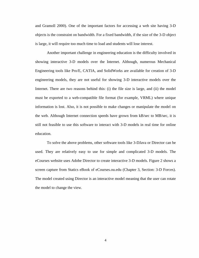
To solve the above problems, other software tools like 3-DJava or Director can be
used. They are relatively easy to use for simple and complicated 3-D models. The
eCourses website uses Adobe Director to create interactive 3-D models. Figure 2 shows a
screen capture from Statics eBook of eCourses.ou.edu (Chapter 3, Section: 3-D Forces).
The model created using Director is an interactive model meaning that the user can rotate
the model to change the view.

5
Figure 2: Example showing use of Director for
displaying 3-D objects
Java programming language can be used to create and display 3-D models over
the Internet. Sun Microsystems developed Java 3-D API to create and manipulate 3-D
geometry over the web (Sun Microsystems). Java 3-D API is a hierarchy of Java classes
and serves as the interface to a sophisticated 3-D graphics and rendering system. Figure 3
shows a screen capture of one of the 3-D game of tic-tac-toe on a 4 x 4 x 4 cube posted
on java.net website.

6
Figure 3: Example showing use of Java3-D for displaying 3-D
objects over the Internet
Although 3-D models can be created and displayed over the Internet using
Director and Java3D, these tools required different plug-ins. For example, the Adobe
Shockwave player plug-in is required for Director to show 3-D objects or the Java plug-in
to display any content created by the Java language. Frequently, neither the students nor
the teachers of the online courses have the computer privilege level to install the required
plug-ins. This situation is more common in industries where companies block unknown
plug-ins for security reasons. Also, after Adobe purchased Macromedia, which owns
Director, there were delays in launching new versions of Director. Because of all these
issues, neither Director nor Java3D was used for this research project (Wikipedia, Adobe
Director).
The next feasible solution was to use Collada file format which is an „open source
format‟ used by Google for their Google Map. But, when this research was started, there
were problems regarding the rendering of 3-D surfaces using Collada. Also, the need to

7
transfer the data from one file format to another to show it on the webpage makes it
difficult to use Collada file format to create 3-D objects.
Another possible solution was to use Adobe Flash for creating 3-D engineering
models. Most personal computers (99% which are connected to Internet) around the
globe have Flash player installed and is free for the user (Adobe Flash Player PC
Penetration 2009). This eliminates the need for the user to download and install a new
plug-in which was a major problem with both Director and Java3D. Flash has a strong a
programming language, ActionScript, that can be used to create and display Flash
models, and uses a special file format for the displaying the models over the Internet,
called „swf‟. The size of the swf files is relatively small; hence, it is suitable to display 3-
D models over the Internet. Because of these advantages, it was decided to use Adobe
Flash for creating interactive 3-D models for this thesis.
1.3 Research Objective
One of the research objectives of this thesis is to develop „Internet-based, user
interactive 3-D engineering models‟. The 3-D models should be easily displayed over the
Internet and should have user interaction facility. The file size of the 3-D model should
be as small as possible so that it does not take excessively long time to load a web page
The second objective is to check the feasibility of Adobe Flash CS3 (henceforth
referred to as Flash), to display 3-D models. Currently, Flash is mainly used for
displaying user interactive 2-D objects over the Internet. When this research started, the
3-D capabilities in Flash were primitive and not conducive for modeling requirements of
engineering industry.

8
Another research objective is to demonstrate collision detection of 3-D models in
Flash. The collision detection technique will help engineering students while doing
assembly of 3-D engineering models. Modeling this problem was especially challenging
since there were no books available and there are few researchers who are working on 3-
D Flash.
Adobe Flash was selected to create interactive web-based 3D models since its
scripting language, ActionScript, can handle vector mathematics. Further, file size is
small and it can be displayed over the web pages to demonstrate 3D modeling
capabilities. A 3D cone shaped funnel (referred to as „cone‟ in this thesis) was created in
Adobe Flash, using Sandy3D engine as shown in Figure 4. The cross-section of the 3D
cone is a Bezier curve whose end control points are fixed and the middle control points
can be manipulated by users. A sphere that rolls along the inner surface of the cone was
used to demonstrate the collision detection technique (not shown in Figure 4).
Figure 4: Different views of a 3-D cone created in Adobe Flash

9
1.4 Thesis Outline
The thesis includes eight chapters, including the current one, and three
appendices. Chapter two reviews the literature related to this research. It also talks about
the reason behind selecting Sandy 3-D engine among all the available Flash 3-D engines.
Chapter three discusses about the parametric modeling, which is the basis for this
research. It also demonstrates how Bezier curve are drawn and the constraints imposed on
the Bezier curve.
Chapter four presents different techniques available to create 3-D models inside
Adobe Flash and then talks more about the Sandy3-D Flash engine chosen for this
research. It then discuss briefly about how a complex shape like 3-D cone can be created.
In modeling 3-D objects, collision detection is an important consideration. Hence
finding the position of a 3-D object with respect to another 3-D object is important. This
is discussed in Chapter five. It also talks about how to find the slope of a 3-D object.
Chapter six talks about the algorithm used to determine motion detection of a 3-D
object with respect to other 3-D object. Chapter seven talks about the results of this
research work and also give the snapshots of the actual running program. Chapter eight
presents conclusions and also talks about the future work needed to be done in this
research field.
The three appendices show the coding for the more important functions written in
ActionScript 3.0.

10
Chapter 2
Literature Review
This research introduces the development of interactive 3-D engineering models
using Adobe Flash CS3 and independent classes from Sandy (Sandy 3D engine 2007).
Sandy is an open source library of ActionScript classes useful for creating 3-D surfaces.
At the commencement of this research work, Adobe Flash lacked true 3D capabilities.
The new Flash version (Flash CS4) has limited 3-D facility which can be used for
modeling basic 3-D objects like 3-D name plates. Also, Flash CS4 gives a 3-D feeling to
some of the 2D objects by changing their depth perception. Change in depth perception is
achieved by making the object look smaller in size as it goes away from the user but the
object itself is not in 3-D. There are different ways for creating 3-D engineering models
like Pro/E, CATIA, AutoCAD; but none of those efforts were directed towards the
creation of interactive web-based 3-D engineering models.
The use of Adobe Flash for creating 3-D engineering models was a major
challenge in this research work since there was no published literature or reliable online
resources. To help solve this issue, open source 3-D engines were created by different
developers. While these are a good starting point, these lack the standardization, and
support that are characteristic of a typical software product launched by a corporation. In
open source technology, all code is open to the developer and they do not need special
permission to use or modify the code from the creator of that technology. Open source
technology also kindles horizontal development, meaning, instead of developing
complete technology by a single person or organization, different ideas came from
various program developers working globally and the product gets more advanced. If one

11
branch of idea is growing faster than the other, then the first group may join in
developing that idea, and thus, helps in developing the whole technology in a faster way.
The drawback is that different developers might be working on the same problem from
different places, so it may waste time and money by engaging more developers
(Wikipedia, Open Source). Still, because of the advantages, open source technologies are
commonly used in the development of 3-D Flash engines. The operating system Linux
and browser Firefox are other prominent examples of open source software collaboration.
The outcome from an open source technology is generally new and it is always
evolving. Hence it is hard to find printed materials or books. When this research started,
there were only a handful of Flash 3-D engines on the development including
PaperVision3D, Away3D and Sandy3D. While the availability of software code was
helpful, there were no books which offered insight into 3-D modeling using Flash. The
availability of the code helped the author to understand the basic concepts of creating 3-D
surfaces inside Flash. This was also crucial in understanding the state of the art and
determining scope and direction of this research.
During the review of these open source codes, it was observed that all 3-D
engines were capable of modeling basic 3-D objects. While the methods used were
different, their overall modeling capabilities were quite similar. For example, all engines
were able to create a planar surface based on coordinates of vertices and direction of the
normal to that surface. The selection of 3D engine for Flash was made by comparing
Papervision3D, Away3D, and Sandy3D against different criteria mentioned in following
paragraphs.
12
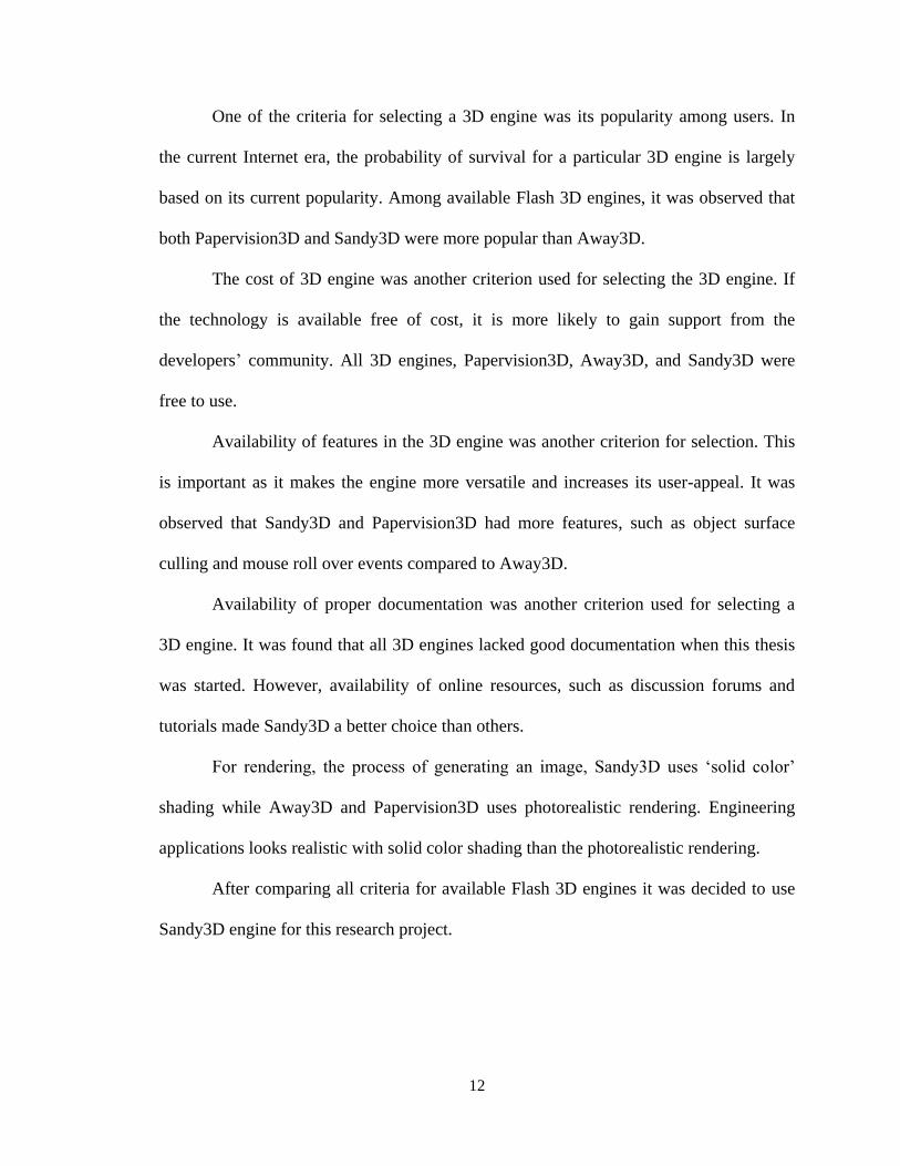
One of the criteria for selecting a 3D engine was its popularity among users. In
the current Internet era, the probability of survival for a particular 3D engine is largely
based on its current popularity. Among available Flash 3D engines, it was observed that
both Papervision3D and Sandy3D were more popular than Away3D.
The cost of 3D engine was another criterion used for selecting the 3D engine. If
the technology is available free of cost, it is more likely to gain support from the
developers‟ community. All 3D engines, Papervision3D, Away3D, and Sandy3D were
free to use.
Availability of features in the 3D engine was another criterion for selection. This
is important as it makes the engine more versatile and increases its user-appeal. It was
observed that Sandy3D and Papervision3D had more features, such as object surface
culling and mouse roll over events compared to Away3D.
Availability of proper documentation was another criterion used for selecting a
3D engine. It was found that all 3D engines lacked good documentation when this thesis
was started. However, availability of online resources, such as discussion forums and
tutorials made Sandy3D a better choice than others.
For rendering, the process of generating an image, Sandy3D uses „solid color‟
shading while Away3D and Papervision3D uses photorealistic rendering. Engineering
applications looks realistic with solid color shading than the photorealistic rendering.
After comparing all criteria for available Flash 3D engines it was decided to use
Sandy3D engine for this research project.

13
Chapter 3
Parametric Modeling
Geometric modeling is widely used in the creation and manipulation of shapes,
particularly in three dimensions. Geometric modeling is an important step in the
engineering design process and it helps to overcome the problems encountered with the
use of physical models (Lee 1999). Parametric modeling, introduced by Parametric
Technology Corporation (PTC), is a type of geometric modeling where a desired shape is
obtained by changing the parameters of the object, like geometric constraints and/or
dimension data (Paramteric Modelling History 2005). Geometric constraint is the relation
between different shape elements such as parallel or perpendicularity between two lines.
The dimension data, provided by the designer, includes the information about the
dimensions assigned to the shape as well as relations between the dimensions which are
expressed in mathematical form. In summary, parametric modeling constructs a shape by
solving the mathematical equations involving geometric constraints.
Parametric modeling generally involves some basic steps to construct a shape.
Firstly, two-dimensional shape is formed in a rough manner. Geometric constraints and
dimensional data are added to the created shape. The shape is reconstructed using these
added parameters. This step is repeated as more and more data is added to the shape.
Then 3-D shape is created by sweeping or rotating this parametric model. As parametric
modeling is linked with data management and collaboration to improve the product
development process, it has remained an important step in the mechanical designing of
the component (Paramteric Modelling History 2005). Because of all these advantages it
was decided to use parametric modeling techniques, to create 3-D model, for this thesis.

14
3.1 Curves in Parametric Modeling
The „curve‟ geometry is one of the primary used geometries for creating
engineering models. Most of the CAD software uses a curve of degree three, represented
by a cubic equation. Two or more cubic curves can be combined seamlessly as second
derivatives of the curves matches with each other. The same continuity can be obtained
for higher degree curves but small oscillations in curve shape may occur. Also additional
computation is required for higher degree curves (Lee 1999). Hence, it was decided to
use curve of degree three for this thesis.
The parametric equation of degree three involves four geometric
coefficients, , , and which can be written as shown in (3.1) and is called a
Hermite curve equation.
Even though the Hermite equation allows curve modification with the geometric
parameters, like tangent at the end points, it is not easy to predict the curve shape as the
magnitude of the tangent vectors, and increases (Lee 1999). To overcome this
drawback, a French engineer Pierre Bezier suggested a new curve, which is called a
Bezier Curve (Wikipedia, Bezier Curve). A Bezier curve is a parametric curve defined by
the vertices of a polygon, called control points, which encloses the resulting curve. The
Bezier curve always passes through the first and the last control point and it is tangent
with the first and the last line segments of the control polygon at the start and the end
(3.1)
15
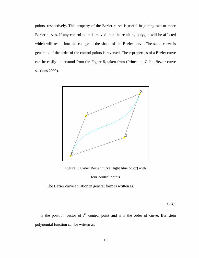
points, respectively. This property of the Bezier curve is useful in joining two or more
Bezier curves. If any control point is moved then the resulting polygon will be affected
which will result into the change in the shape of the Bezier curve. The same curve is
generated if the order of the control points is reversed. These properties of a Bezier curve
can be easily understood from the Figure 5, taken from (Princeton, Cubic Bezier curve
sections 2009).
Figure 5: Cubic Bezier curve (light blue color) with
four control points
The Bezier curve equation in general form is written as,
is the position vector of ith
control point and n is the order of curve. Bernstein
polynomial function can be written as,
(3.2)

16
and
For a Bezier curve of degree equal to three (n = 3), the number of control points
are (n + 1) four. By substituting n = 3 and doing some simple mathematics, the Bezier
curve equation in Matrix form can be written as,
where and are control points of the Bezier curve.
Complicated curves can be formed by moving the control points of the Bezier
curve as shown in the Figure 6.
Figure 6: Twisted Bezier curve (light blue color) with
four control points
(3.3)

17
3.2 Curve Restrictions Imposed
Certain positions of the control points may produce a surface that is twisted or
warped when the Bezier curve is as shown in Figure 6 hence; it was decided to impose
restrictions on the movement of the control points for this thesis without compromising
the complexity of the curve obtained. The end control points (red color) of the Bezier
curve were fixed at top most right corner as well as bottom most left corner of the
polygon. Also, movement of the inside control points (blue color) is restricted. Point 1
will always remain above the bottom most left corner (Point 0) and below the top most
right corner (Point 3) of the polygon. The similar restrictions will apply for other
movable control point, Point 2. Also, control Point 1 cannot go to the left side of the end
control point, Point 0 and it cannot go to the right side of the control Point 2. Similar
restriction for control Point 2, that is, Point 2 cannot go the right side of the end control
Point 3 and also it cannot go to the left side of the control Point 1 is applied. The resulted
restrictions for Point 1 and Point 2 are shown with green and orange color respectively in
Figure 7.
Figure 7: Restriction imposed for creating
Bezier curve

18
Different Bezier curves obtained with the restrictions are showed in the Figure 8.
Figure 8: Different Bezier curves obtained after restrictions imposed on control points
The actual plotted curve is obtained by joining small segments along the Bezier
curve. The curve becomes smoother as the numbers of segments increases. But as the
number of segment increases, there is also an increase in the calculations which may
result in the sluggish operation of the 3-D modeling tool. Since, the curve will be rotated
to construct the 3-D cone, the total number of surfaces and thus calculations can quickly
multiple out of control. So, the number of segments for a Bezier curve was restricted to a
maximum sixteen.

19
Chapter 4
3-D Modeling Using Adobe Flash
Although Adobe Flash CS3 itself does not have native 3-D capabilities, it can
display vector based shapes and can handle mathematical calculations which can be used
to show 3-D models. Generally, it is accomplish in one of two ways, creating 3-D objects
outside the Flash and bringing them back in as a pre-rendered 3-D object or by
dynamically creating the models mathematically as 3-D objects using ActionScript.
With the pre-rendered option, the developer can use Swift 3-D, which will render
out 3-D scenes created within its environment and then exported into „swf‟ files, movie
files, or just sequential images which can be imported and manipulated by Flash.
Sometimes users even do not need to use Flash. This is one of the best solutions for 3-D
animated movies but it can limit the user-interactivity with the 3-D object which is one of
the objectives of this thesis.
The other option of creating 3-D objects dynamically requires basic vector
mathematics for handling 3-D rendering. Since Flash can perform mathematics,
developers can create 3-D models dynamically. Depending upon the complexity of 3-D
users want to show, the mathematics involved may become more complicated. Different
open source 3-D engines have been created for 3-D modeling in Flash. Their benefit is
that they are open source, so any one can modify the source code as needed.
Papervision3D is one of the Flash 3-D open source engines that create and display
3-D in Adobe Flash. The main advantage of Papervision3D is it can handle „collada‟ file
format to display 3-D. Collada files format is used by Google to show 3-D images inside
Google Earth software. But two drawbacks of Papervision3D, is it cannot render solid

20
colors which gives feel of solid engineering model and the lack of documentation. Hence,
Papervision3D was not used for this thesis.
Away3D is another 3-D engine available for creating 3-D using Adobe Flash.
Although, it has solid colors, it lacked good documentation and hence it was not the used
for creating 3-D models.
The other major open source 3-D engine available was Sandy3D. It solved both
the problems, namely, it has solid colors and there are reasonable amount of
documentation available. Sandy3D can handle around 2,000 – 5,000 polygons on a
common duo-core Intel processor computer (Sandy 3D engine 2007). This was one of the
major factors for selecting the 3-D engine since engineering shapes are complicated and
require more polygons to display the 3-D object.
4.1 Sandy Pipeline Running Behind
In Sandy3D, the geometry is first created using a basic class. Then the actual
geometry is attached to a 3-D shape. This step also includes the creation of 3-D vertices.
Each vertex gets a unique ID and then using these vertices (three or four) different 3-D
surfaces are created. A new surface IDs is assigned to the surface and „appearance‟ with
„material‟ properties is created. Different properties like, color, outline, and the „alpha‟
property, used for „opacity‟, of the 3-D surfaces are associated with „material‟. The two
materials are required for the front and back side of a single polygon.
The rear surface is not displayed if it goes behind another surface. This is known
as „back face culling,‟ and is used to detect whether surface is behind any other the
surface or not. Depending upon the answer, the display calculations are done. This saves
CPU usage if there are a large number of surfaces. The „appearance‟ is linked to the

21
„shape‟ namely, cube, sphere, and cylinder. Each polygon of that „shape‟ will have its
own „appearance‟.
All 3-D models are displayed using „scene‟ (Scene 3-D object from Sandy‟s
library) and a „camera‟ is attached to it. A „camera‟ is the viewer‟s eye which is
positioned in a space using x, y, and z coordinates. A „camera‟ can be a static object
looking at a stage or it can be a dynamic object which can rotate, roll, or tilt around the
other 3-D models. A 3-D model can be seen from all sides either by moving it or by
moving the „camera‟. The user can use it in either way, but it is better to move the camera
if the stage is holding a large number of 3-D objects. The user can set the light direction,
by setting the x, y, z co-ordinates of the light source. Because of this 3-D model appears
like a „real object‟ as some part of it will have bright surfaces and others will have darker
depending upon the position of the light source.
Sandy3D also has a „World 3-D‟ object which can be used as a stage for
displaying all 3-D models. The drawback of using „World3-D‟ object is that, the user
cannot move one 3-D object with respect to another 3-D object. User need to delete both
3-D objects and then draw/render again. This process works well if there are less 3-D
surfaces present on the stage. But, as the number of 3-D surfaces increases, the time
requiring for rendering those 3-D surfaces increases and the animation look sluggish.
Because of this, all 3-D models are created using „Scene 3-D‟ objects for this thesis.
4.2 Procedure to Display 3-D Objects
Once the scene is created, still there are four steps needed to display the 3-D
object. The first one is to update the local transformation of each transformable node. The
second step is to compute the scene tree transformation concatenation and proceed to the
22
culling of objects/surfaces if it is not visible. This step will save the processor time for
showing a 3-D model. The third step, rendering, is vital to show the geometry
transformation. If the user does any modification, such as, rotate the object, then
rendering again is essential. If this step is forgotten then old 3-D objects will be
displayed. There might be a possibility that all calculations for new positions are done,
but is not displayed because this step is missing. The next step is of displaying the
material which will show the polygons associated with it. This step is an integral part of
the rendering step.
4.3 Creation of 3-D Cone
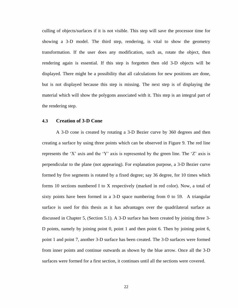
A 3-D cone is created by rotating a 3-D Bezier curve by 360 degrees and then
creating a surface by using three points which can be observed in Figure 9. The red line
represents the „X‟ axis and the „Y‟ axis is represented by the green line. The „Z‟ axis is
perpendicular to the plane (not appearing). For explanation purpose, a 3-D Bezier curve
formed by five segments is rotated by a fixed degree; say 36 degree, for 10 times which
forms 10 sections numbered I to X respectively (marked in red color). Now, a total of
sixty points have been formed in a 3-D space numbering from 0 to 59. A triangular
surface is used for this thesis as it has advantages over the quadrilateral surface as
discussed in Chapter 5, (Section 5.1). A 3-D surface has been created by joining three 3-
D points, namely by joining point 0, point 1 and then point 6. Then by joining point 6,
point 1 and point 7, another 3-D surface has been created. The 3-D surfaces were formed
from inner points and continue outwards as shown by the blue arrow. Once all the 3-D
surfaces were formed for a first section, it continues until all the sections were covered.

23
Figure 9 : Cone creation by rotating a Bezier curve
After taking the input for number of sections and number of line segments in a
Bezier curve from the user, the code develops the 3-D cone dynamically.

24
Chapter 5
Detection of a 3-D Object on a Surface and Finding the
Slope of a Surface
Collision detection is an important aspect for creating 3-D models by checking
whether a 3-D object is touching or intersecting with another. Since all the engineering
objects are generally solids and interaction between them can be modeled using dynamic
constraints and contact analysis, it is important to involve a collision detection algorithm
in this thesis. Since the physical simulations need to simulate the real world physics as
precisely as possible, it is important to include the collision detection techniques in real
time. A virtual object can feel solid and it is possible to find the relative position of a 3-D
object with respect to other using the collision detection. In this thesis, this technique is
used to identify the sphere position respective to different 3-D surfaces created for the
cone. Once the 3-D surface is identified then the sphere can be moved depending upon
the slope of the 3-D surface and the initial velocity of the sphere.
5.1 Importance of a Triangular Surface for Creating a 3-D Surface
Sandy3D can create 3-D surfaces using four points (quad-surface) or by three
points (triangular surface). It is difficult to find the plane of a 3-D quad-surface as four
points can belongs to a single plane or lie in different planes. This will not be the case for
triangular surfaces as all of its vertices would always define one and only one plane.
Hence, triangular surfaces are used for creating the 3-D surfaces in this thesis. This
property also helped in finding the slope of the 3-D surface, essential for moving the
sphere inside the 3-D funnel shaped cone created using a large number of small 3-D

25
triangles. Different ways for finding the position of the sphere respective to the 3-D
triangle are discussed in the following paragraphs.
5.2 Sphere Inside the Triangle
A common way to check whether the sphere lies inside a triangle is by treating
the sphere as a point and then finding the vectors connecting the point to each of the
triangle vertices. If the sum of the angles is 360 degrees then the sphere lies inside the
triangle. This technique is easy to understand but slow in execution and hence cannot be
implemented for this thesis (Blackpawn.com 2001). The different techniques which
would give the results faster are discussed in the following paragraphs.
Area Technique
In an area technique, a point is connected to three vertices of the triangle and three
different triangles, namely, triangle APC, triangle BPA, and triangle CPB are formed as
shown in Figure 10.
Figure 10: Area technique to determine
whether point is inside the triangle

26
Then, area of three triangles is calculated and equated it to with the area of the
original triangle as shown,
The point lies inside the triangle if the condition in (5.1) is satisfied. The
disadvantage of an area technique is the high CPU time required to determine the area of
four triangles which determines whether the point lies inside a single triangle. Since the
code for the 3-D cone have large number of triangles, this process will consume a
considerable amount of time. Hence, this technique is not used for determining whether
the sphere is inside the 3-D triangle.
Same side Technique
In this technique, the point will be inside the triangle if it is on the same side of
each edge of the triangle. This can be explained by forming a triangle (yellow) by three
lines, AB, BC, and CA as shown in Figure 11. Lines, AB, BC and CA each split the
space in half, and one of those halves is entirely outside the triangle. For a point to lie
inside the triangle ABC, it must be below AB, left of BC and right of CA.
Figure 11: Same side technique to determine
whether point is inside the triangle
(5.1)

27
Cross product technique can be used to determine whether the point is on the
correct side of a line or not as shown in Figure 12. The cross product of (B – A) and (P‟ –
A) will be a vector pointing outside the plane, and the cross product of (B – A) and (P –
A) will be a vector pointing inside the plane. The correct direction of the vector is
determined with the help of the third point of a triangle, point C. If the cross product of
(B – A) and (P – A) is pointing in the same direction as the cross product of (B – A) and
(C – A), then point P is on the correct side of the line AB.
Figure 12: Cross product technique for
determining point position
If the point is on the same side of AB as C, on the same side of BC as A, and on
the same side of CA as B, then it is inside the triangle. This process involves at least six
cross products for one surface and there will be large number of surfaces involved in
creating a single 3-D cone. Hence, this technique is not used to determine whether the
point lies inside the 3-D triangle.
Barycentric Technique
Since the three points of the triangle defines a plane in space, by choosing one
point as a reference, the co-ordinate of any point can be found relative to that point using

28
two vectors. Using these vectors and it is possible to determine whether the point lies
inside the triangle.
For example, taking point A as our reference point and the two edges that touch
A, (C – A) and (B – A) as basis vectors, as shown in Figure 13, the user can determine
the co-ordinate of any point P as shown,
where the conditions of the point P to be inside the triangle are,
Figure 13: Barycentric technique - checking point
position (condition - 1)
To find the values of u and v from equation (5.2), some simple mathematics are
required as shown below,
(5.2)
(5.3)

29
Let , , and . So the above equation, (5.4)
can be written as,
To get the values of unknowns, and , two equations are needed, which can be
obtained by doing a dot product on both sides by and
Solving the above two equations, the values of and are obtained as,
This technique can be easily understood using a Flash interactive example
(Blackpawn.com 2001). If the point is outside the triangle, the value of u is less than one
which can be observed in Figure 13 (here ).
Both and are positive when the point is inside the triangle. Also, notice
that . This condition is shown in Figure 14.
(5.4)
(5.5)
(5.6)
(5.7)

30
Figure 14: Barycentric technique - checking
point position (condition - 2)
If the point is outside the triangle, as shown in the Figure 15, then although the values of
u and v are both positive, it does not satisfy the third condition as 1.
Figure 15: Barycentric technique - checking
point position (condition - 3)

31
Although, Barycentric technique involves some more mathematics, it is easy to
understand and relatively faster to execute, which is one of the requirements of this thesis
due to the large numbers of triangular surfaces involved for a 3-D surface. Hence,
Barycentric technique method was selected for this thesis.
5.3 Finding the Slope of 3-D Surface
The new sphere location for next time interval is determined after confirming that
it is inside the triangle. The new sphere location depends upon; initial position, initial
velocity and slope of the triangle. The slope of the triangle can be determined by finding
the slope of the 3-D plane passing through the three vertices of it. This is illustrated in the
Figure 16. After knowing the co-ordinates, the normal to that triangle is calculated by
taking the cross product of any two edges, say, and , having a common vertex, .
For the illustrated example cross product of represents the normal to the 3-D
plane shown in orange color. Then the cross product of the gravity vector (g) in the
direction of z (not shown) and the normal vector of the 3-D surface (orange color) is
calculated and is shown in green color. The cross product of this vector (green vector)
and the vector normal to the plane (orange vector), shown in red color in the Figure 16,
gives the slope of the 3-D triangle.

32
Figure 16: Finding the slope of a 3-D surface
Once the slope of a 3-D surface is known then the sphere will move in that
direction for the next time increment. The new velocity of the sphere, v can be calculated
by using the initial velocity and this slope vector, , as shown,
(5.8)
where, is final velocity of the sphere, is initial velocity of the sphere, is acceleration
of the sphere and ∆t is time increment between initial and current state. The new position
of the sphere can be found using this velocity as,
(5.9)
where, and is final and initial position of the sphere respectively. Since is small,
the last term is ignored and the new sphere position is found by,
(5.10)
33
Chapter 6
Motion Detection between a 3-D Object and a 3-D Surface
A 3-D funnel shaped cone‟s surface is created using a number of small triangles.
The new position of the sphere depends on slope of the triangular surface in which it is
lying, velocity and the initial position of the sphere. Different approaches for moving the
sphere inside the cone are discussed in following paragraphs.
6.1 Find the 3-D Surface and Move the 3-D Sphere Approach
In this approach the initial 3-D triangle in which the sphere is laying, called the
“parent triangle”, is determined. The sphere is moved by calculating the slope of the
parent 3-D triangle. These two things, finding the parent triangle and finding the slope of
the 3-D triangle, are done repeatedly to move the sphere inside the 3-D cone. The
flowchart for this approach is illustrated in Figure 17.

34
Find the triangular
surface in which the
sphere is residing
Make that triangle
as a parent
triangle
Find the slope of
the parent triangle
Find the new position of
the sphere using the
slope, initial velocity.
Is the sphere
position is inside
the triangle?
Yes
Stop
No
Start
Figure 17: Flowchart for finding the slope of 3-D surface
and moving the 3-D sphere approach
The program take too much time to find out the triangular surface in which the
sphere is laying as complicated surfaces are formed by large number of 3-D triangles.
Hence, this approach was not used for moving the sphere inside the 3D cone.
6.2 Find the Adjacent Triangles of the Parent Triangle Approach
In this approach, the adjacent triangles of the parent triangles are determined and
once the sphere is outside the parent triangle then these adjacent triangles are checked to
determine if they contain the sphere. Determining the adjacent triangles is done by
naming each node/vertex of a 3-D surface by a unique number and then finding all
triangles which consists one of the parent triangle nodes. Once the 3-D sphere moves out
of first parent triangle, the program will only check for the neighboring triangles. If the

35
difference between the new position of the sphere and the initial position of the sphere,
step size, is small than the size of the 3-D triangular surface then the sphere will lay in the
neighboring triangles once it leaves the parent triangle. This approach reduces a
computational work by doing fewer calculations and hence can be used for a surface
having large number of triangles. The flow chart for this approach is shown in Figure 18.
Find the triangular
surface in which the
sphere is residing
Make that triangle
as a parent
triangle
Find the slope of
the parent triangle
Find the new position of
the sphere using the
slope, initial velocity.
Is the sphere
position is inside
the triangle?
Yes
Stop
No
Is the sphere is
inside the adjacent
triangle?
Yes
No
Start
Figure 18: Flowchart for find the adjacent triangles of the
parent triangle approach

36
A 3-D cone consists of a large number of triangular surfaces oriented in
differently in 3-D space and this method did not have solution for transferring the sphere
to those surfaces. Hence, this method is not suitable for moving the sphere inside the 3-D
cone.
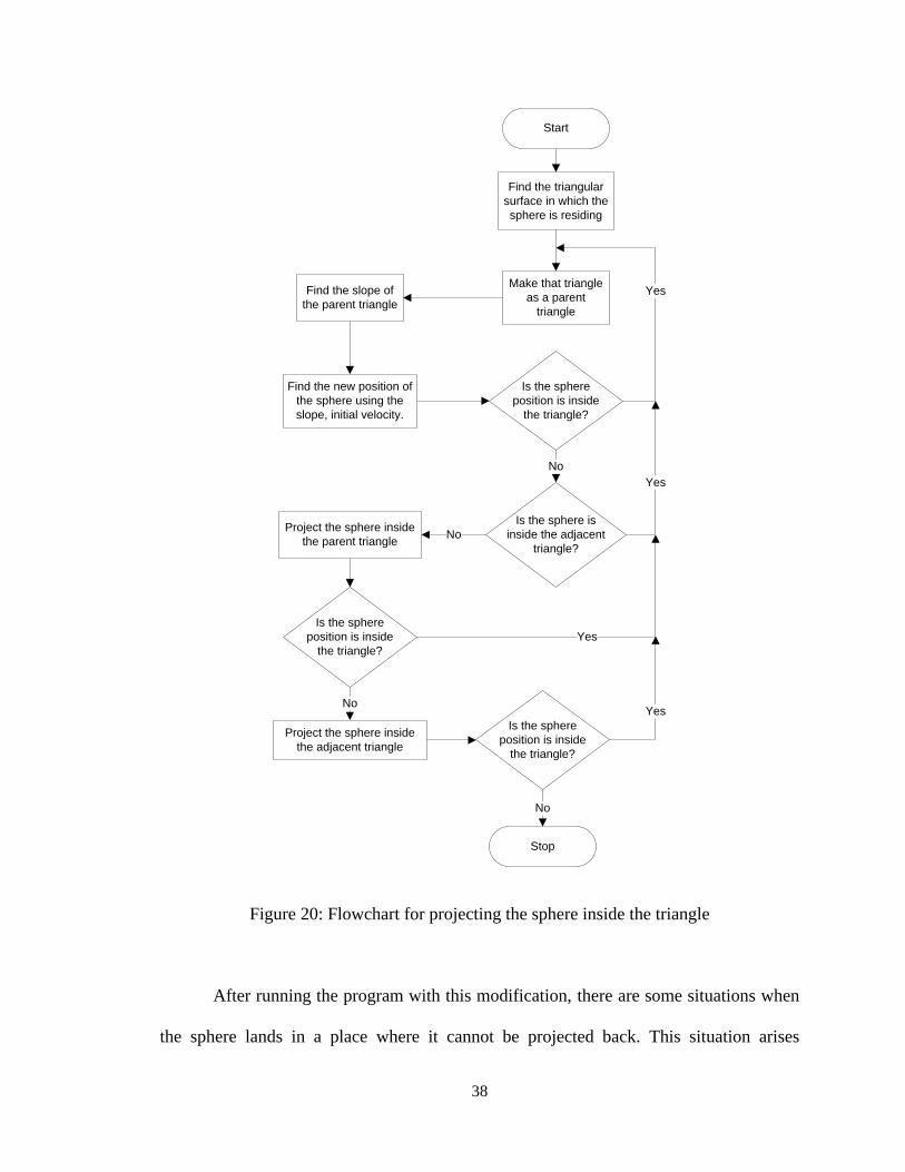
6.3 Projecting the Sphere inside the Triangle Approach
As discussed earlier in Chapter 4 (Creation of 3-D Cone3-D Modeling Using Adobe
Flash), a 3-D cone is formed by rotating a Bezier curve which consists of small segments.
Hence, all 3-D triangles are not in a single plane. As the 3-D sphere leaves a parent
triangle ABD it is supposed to go inside the other triangle BCD. But, the triangle BCD is
oriented differently in 3-D space. So, the sphere lands in a space (B‟) which is not
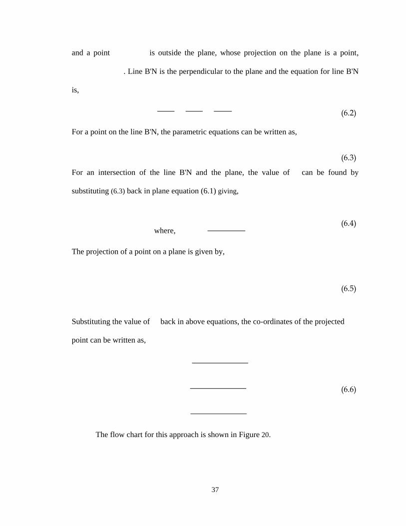
included in any triangle as shown in the Figure 19.
Figure 19: Projecting a point on a plane
To overcome this problem, a function is added which would project the sphere
inside the plane using a simple calculations. Consider the equation of plane (p) as
(6.1)
37
and a point is outside the plane, whose projection on the plane is a point,
. Line B'N is the perpendicular to the plane and the equation for line B'N
is,
(6.2)
For a point on the line B'N, the parametric equations can be written as,
For an intersection of the line B'N and the plane, the value of can be found by
substituting (6.3) back in plane equation (6.1) giving,
where, (6.4)
The projection of a point on a plane is given by,
(6.5)
Substituting the value of back in above equations, the co-ordinates of the projected
point can be written as,
(6.6)
The flow chart for this approach is shown in Figure 20.
(6.3)
38
Find the triangular
surface in which the
sphere is residing
Make that triangle
as a parent
triangle
Find the slope of
the parent triangle
Find the new position of
the sphere using the
slope, initial velocity.
Is the sphere
position is inside
the triangle?
Yes
Stop
No
Is the sphere is
inside the adjacent
triangle?
Yes
NoProject the sphere inside
the parent triangle
Is the sphere
position is inside
the triangle?
Project the sphere inside
the adjacent triangle
Yes
No
Is the sphere
position is inside
the triangle?
No
Yes
Start
Figure 20: Flowchart for projecting the sphere inside the triangle
After running the program with this modification, there are some situations when
the sphere lands in a place where it cannot be projected back. This situation arises

39
because of the orientation of certain triangles as shown in Figure 21. Assumed the sphere
is rolling from triangle ABC along the edge AB. After the sphere leaves triangle ABC
somewhere near point B, it‟s new position is point P. After projecting the sphere on the
plane same as triangle BDC, the new position will be point P‟. Point P‟ is in the same
plane as triangle BDC but it is outside the triangle BDC.
Figure 21: Black-hole position for a 3-D sphere
The sphere projection is not possible in this situation, referred as a black hole
situation. Hence this method was not used to move the sphere inside the 3-D cone.
6.4 Restricting the Sphere inside a Triangle Approach
In this approach, after finding the new position for the sphere the program checks
whether the new position of the sphere is inside the parent triangle. If it is inside the
triangle, then the sphere‟s new position is updated. But, if the sphere‟s new position is
outside the parent triangle then the program finds out the edge of the parent triangle from
where the sphere exited. Once that edge is found out, the sphere location is updated at the
point where the sphere leaves the parent triangle. Then the adjacent triangle to that edge
is searched, and that adjacent triangle will become the parent triangle for the next
iteration. Velocity vector is projected on this new parent triangle. Searching of new
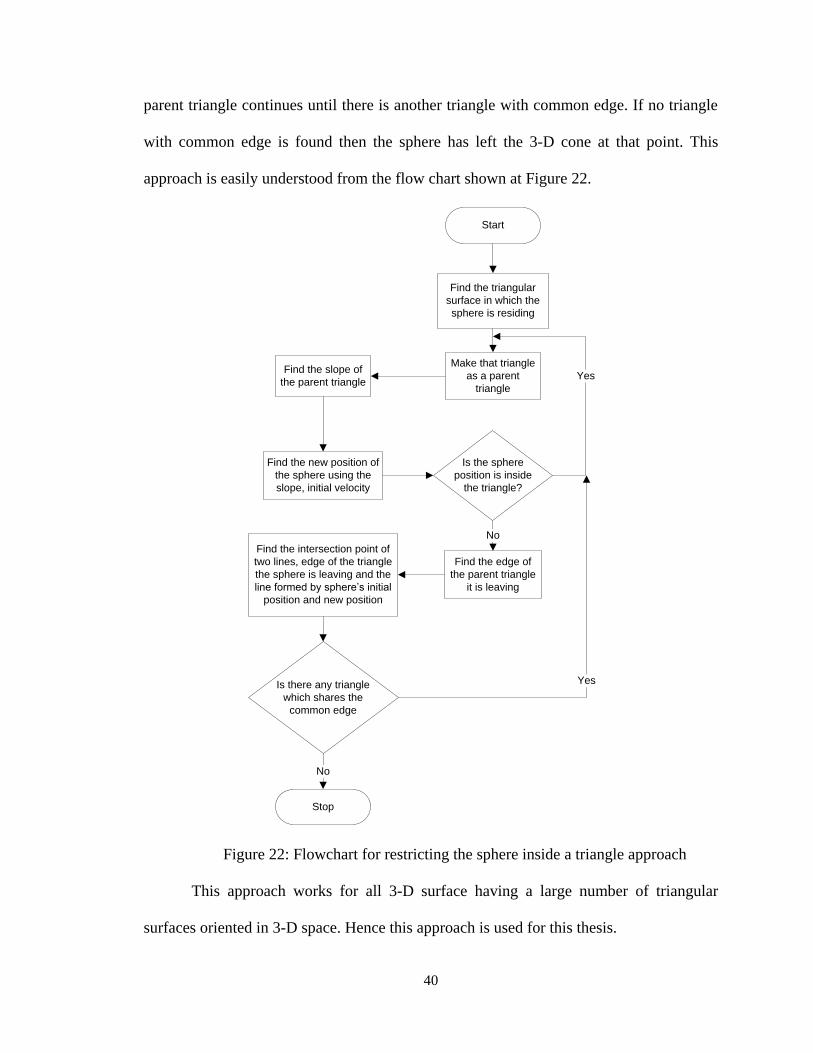
40
parent triangle continues until there is another triangle with common edge. If no triangle
with common edge is found then the sphere has left the 3-D cone at that point. This
approach is easily understood from the flow chart shown at Figure 22.
Find the triangular
surface in which the
sphere is residing
Make that triangle
as a parent
triangle
Find the slope of
the parent triangle
Find the new position of
the sphere using the
slope, initial velocity
Is the sphere
position is inside
the triangle?
Yes
Stop
Is there any triangle
which shares the
common edge
No
Find the edge of
the parent triangle
it is leaving
Find the intersection point of
two lines, edge of the triangle
the sphere is leaving and the
line formed by sphere’s initial
position and new position
No
Yes
Start
Figure 22: Flowchart for restricting the sphere inside a triangle approach
This approach works for all 3-D surface having a large number of triangular
surfaces oriented in 3-D space. Hence this approach is used for this thesis.

41
Chapter 7
Testing and Performance
The interactive web-based tool created for this thesis is tested considering
different test scenarios. Some of the test scenarios are discussed in the following
paragraphs.
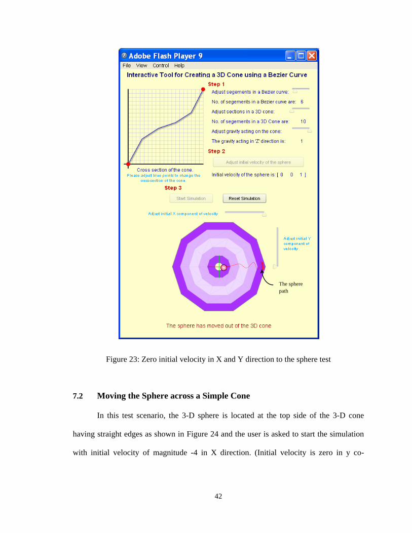
7.1 Zero Initial Velocity in X and Y Direction to the Sphere Test
In this test case, the 3-D sphere is located at the top side of the 3-D cone (default
initial position of the sphere) and the user asked to start the simulation without giving an
initial velocity. (Initial velocity in x, and y co-ordinates is zero.) Since there is no velocity
present in X and Y direction, the sphere is expected to move slowly during initial part of
simulation. The sphere will gain velocity in later part of simulation and is expected to
move out of the cone.
Expected results were obtained from the tool when this test was conducted. The
sphere appears to be stable during the initial period of simulation but gained the velocity
as the time increases and moves fast in later period of the simulation. The path of the
sphere is shown in red color in Figure 23 When the sphere is out of the cone then the
message saying „The sphere has moved out of the 3D cone‟ got displayed as shown in the
Figure 23. The user can change the velocity by using „Adjust initial velocity of the
sphere‟ button from the top. This button was enabled after the user clicks on the „Reset
Simulation‟ button.
42
Figure 23: Zero initial velocity in X and Y direction to the sphere test
7.2 Moving the Sphere across a Simple Cone
In this test scenario, the 3-D sphere is located at the top side of the 3-D cone
having straight edges as shown in Figure 24 and the user is asked to start the simulation
with initial velocity of magnitude -4 in X direction. (Initial velocity is zero in y co-
The sphere
path

43
ordinates). As there is no velocity present in Y direction, the sphere is expected to move
in a straight line and should come out of the cone from the bottom side.
Figure 24: Straight edge cone for test case scenario
Satisfactory results were obtained after conducting this test on the Flash tool. The
sphere moved in „zic-zag‟ pattern, shown in red color in Figure 25, as the sphere was on
the edge of two section of the cone (Please see section 4.3: Creation of 3-D Cone for the
explanation about the sections of the cone). As the sphere moved down from the top, it

44
actually shifted from one section to other and vice-versa depending upon the slope of the
triangle in which the sphere was positioned. The „zic-zag‟ pattern was observed as the
step size, difference between new position of the sphere relative with the earlier position
of the sphere, increases. When the sphere reached the bottom of the cone then the
message saying, „The sphere has moved out of the 3-D cone‟ got displayed as shown in
Figure 25.
Figure 25: Moving the sphere across a straight line cone.
The sphere
path

45
7.3 Moving the Sphere across the Cone with Initial Velocity in X and Y
Direction
In this test scenario, the 3-D sphere is located at the top side of the 3-D cone and
the initial velocity in both X and Y direction is given. Then the user asked to start the
simulation. The expected result from this test case scenario is that the sphere should
move down in a curve path depending upon the magnitude of initial velocity and
eventually will get out of the cone.
Actual test results for this scenario matched perfectly to the expected results. The
sphere took a curved path, shown in red color in Figure 26, before going out of the 3-D
cone from the bottom side and the correct message of „The 3-D sphere has moved out of
the cone‟ got displayed as shown in the Figure 26.

46
Figure 26: Moving the sphere across the cone with initial velocity in X and Y direction
7.4 Moving the Sphere across the Cone having ‘U’ section and with Initial
Velocity in X Direction
In this test scenario, the 3-D sphere is located at the top side of the 3-D cone
having a cross section of „U‟ shape. This cross section is obtained by controlling control
points of a Bezier curve. Then initial velocity in only X direction is given and then the
The sphere
path
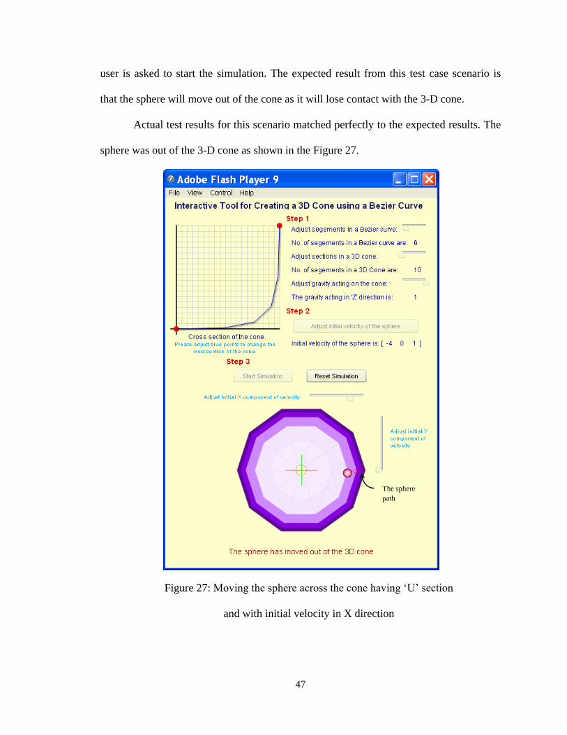
47
user is asked to start the simulation. The expected result from this test case scenario is
that the sphere will move out of the cone as it will lose contact with the 3-D cone.
Actual test results for this scenario matched perfectly to the expected results. The
sphere was out of the 3-D cone as shown in the Figure 27.
Figure 27: Moving the sphere across the cone having „U‟ section
and with initial velocity in X direction
The sphere
path

48
From the results discussed above, it is clear that the tool developed using Adobe
Flash completely satisfies all the research objectives for this thesis.

49
Chapter 8
Conclusion
8.1 Summary
The primary objective of this research was to develop web-based 3-D engineering
simulations. Since there are few studies available for creating 3-D engineering
simulations on a web-based environment, this thesis is a pioneer study in this area. The
major part of this research was spent on developing a code using ActionScript, a scripting
language used by Adobe Flash, for creating 3-D models. The other focus was to develop
a code to detect collision between two 3-D objects using Adobe Flash.
For use to understand 3D dynamics, 3-D funnel shaped cone is created using the
Adobe Flash CS3, Sandy3D, and the ActionScript 3.0 language (part of Flash). The cross
section of the 3-D cone is controlled by the Bezier curve and a sphere is positioned at the
top edge of the cone. The sphere moved inside the 3-D cone depending upon the cross
section of the 3-D cone and the initial velocity given by the user.
The tool developed with all the requirements set for this thesis has the file size of
only 80kB (kilo bytes). Because of such a small size, it is easy to upload on the web page
and there are almost no chances that the user will observe sluggish behavior of the web
page.
The tool developed for this research work was tested extensively by the author
and it satisfies all the expectations puts before this research work has begun. Different
test scenarios are developed and documented in this thesis. There were no major
problems observed during the testing and few recommendations were suggested.

50
8.2 Recommendations and Future Scopes
The primary objective of this research was to develop web-based 3-D engineering
models using Adobe Flash. Although all the objectives of this research were achieved the
author will suggest that more research is still necessary in this field for more efficient
way for creation of 3-D surfaces to reduce the computing time and to display more
complicated 3-D shapes over the Internet.
The author will also recommend using collaborative technique to get all the
benefits from this tool. The research carried out on different collaborative techniques
especially at Engineering Media Lab of University of Oklahoma can be applied for 3-D
engineering models.

51
References
Adobe Flash. Adobe Flash Player PC Penetration. Adobe. March 2009.
http://www.adobe.com/products/player_census/flashplayer/PC.html (accessed September 09,
2009).
Blackpawn.com. Point in triangle test. November 16, 2001.
http://www.blackpawn.com/texts/pointinpoly/default.html (accessed September 21, 2009).
Bourne, J. R., A. J. Brodersen, J. O. Campbell, M. M. Dawant, and R. G. Shiavi. "A Model for
On-Line Learning Networks in Engineerring Education." Journal of Asynchronous Learning
Networks 1, no. 1 (March 1997).
Bourne, John, Dale Harris, and Frank Mayadas. "Online Engineering Education: Learning
Anywhere, Anytime." JALN 9, no. 1 (March 2005): 15-41.
Gramoll, Kurt. eCourses.ou.edu. Edited by Kurt Gramoll. http://ecourses.ou.edu (accessed
September 09, 2009).
Lee, Kunwoo. Principles of CAD/CAM/CAE. Prentice Hall, 1999.
Peterson, George D, and Lyle D Feisel. "e-Learning: The Challenge for Engineering Education."
Edited by Jack R. Lohmann and Michael L. Corradini. 2002 ECI Conference on e-Technologies
in Engineering Education: Learning Outcomes Providing Future Possibilities. Davos,
Switzerland, 2004. 164-169.
Princeton, Cubic Bezier curve sections. Cubic Bezier curve section. November 19, 2009.
http://www.cs.princeton.edu/~min/cs426/jar/bezier.html (accessed September 14, 2009).
Saitz, Robin. Paramteric Modelling History. December 15, 2005.
http://www.mcadonline.com/index.php?option=com_content&task=view&id=177&Itemid=1
(accessed September 13, 2009).
Sandy 3D engine. Sandy 3D engine tutorials. November 11, 2007. http://www.flashsandy.org/
(accessed September 21, 2009).
Sun Microsystems. Java 3D. Sun microsystems. https://java3d.dev.java.net/ (accessed September
09, 2009).
Sun, Qiuli, Kevin Stubblefield, and Kurt Gramoll. "Internet-based Simulation and Virtual City for
Engineering Education." American Society of Engineering Education (ASEE). St. Louis, MS:
American Society of Engineering Education (ASEE), 2000.
Tampone, Kevin. Online Learning Growing in Prominence. September 08, 2009.
http://findarticles.com/p/articles/mi_qa3718/is_200510/ai_n15740171/.

52
Wikipedia, Adobe Director. Adobe Director. Wikipedia .
http://en.wikipedia.org/wiki/Adobe_Director (accessed September 09, 2009).
Wikipedia, Bezier Curve. Bezier Curve. http://en.wikipedia.org/wiki/Bezier_curve (accessed
September 13, 2009).
Wikipedia, Open Source. Open Source - Wikipedia. January 21, 2010.
http://en.wikipedia.org/wiki/Open_source (accessed January 24, 2010).

53
Appendices
Appendix 1: ActionScript code for creating a Bezier Curve
After drawing the control points pt1, pt2, pt3 and pt4 for a Bezier curve, a Bezier Curve is drawn
using the draw_curve function which is shown below,
function draw_curve(event:Sprite):void {// Draw bezier curve using equation (3.3),
//To draw a Bezier curve use the syntax as: var BezCurve:Sprite = new Sprite();
BezCurve.graphics.lineStyle(1.2,0x0000CC,1);
BezCurve.graphics.moveTo(pt1.x, pt1.y);
//Declaring constant variables, which will require in the bezier curve equation.
var const_1 = -1 * pt1.x + 3 * pt2.x + -3 * pt3.x + 1 * pt4.x;
var const_2 = 3 * pt1.x + -6 * pt2.x + 3 * pt3.x + 0 * pt4.x;
var const_3 = -3 * pt1.x + 3 * pt2.x + 0 * pt3.x + 0 * pt4.x;
var const_4 = 1 * pt1.x + 0 * pt2.x + 0 * pt3.x + 0 * pt4.x;
var const_5 = -1 * pt1.y + 3 * pt2.y + -3 * pt3.y + 1 * pt4.y;
var const_6 = 3 * pt1.y + -6 * pt2.y + 3 * pt3.y + 0 * pt4.y;
var const_7 = -3 * pt1.y + 3 * pt2.y + 0 * pt3.y + 0 * pt4.y;
var const_8 = 1 * pt1.y + 0 * pt2.y + 0 * pt3.y + 0 * pt4.y;
var z:Number = 1;
for (var k:Number = 0; k <= 1; k = k + (1 /Parts)){
points_array_x[k] = [Math.pow(k,3)* ( const_1)+ Math.pow(k,2)* ( const_2)+
Math.pow(k,1)* ( const_3)+ Math.pow(k,0)* ( const_4)];
points_array_y[k] = [Math.pow(k,3)* ( const_5)+ Math.pow(k,2)* ( const_6)+
Math.pow(k,1)* ( const_7)+ Math.pow(k,0)* ( const_8)];
event.graphics.lineTo(points_array_x[k],points_array_y[k]);
//The following information will be used later in drawing the cone again.
interRad[k] = "Radius " + z;
radZ[z] = points_array_y[k];
interRadValue[z] = points_array_x[k];
trace("Internal radius " +interRad[k]+ " is " +interRadValue[z]);
z++;
}
event.graphics.lineTo(pt4.x,pt4.y);
BezCurve.filters = [CurveShadow]; //Drawing a shadow of curve.
//Attaching curve to 'Graph' sprite for display on stage
Graph.addChild(event);
}

54
Appendix 2: ActionScript code for creating 3-D Cone
The ActionScript code to draw a 3-D cone is shown below. All the comments are shown in grey
color.
/*
This code generates cone if 4 points are given in a row.. (If points are linear then it will be plane
cone and if points are non-linear then cone will have curve cross-section).
Cone3-D = new Pipe3-D( "Title", Point1 X co-ordinate, Point1 Y co-ordinate, Point2 X co-
ordinate, Point2 Y co-ordinate, Point3 X co-ordinate, Point3 Y co-ordinate, Point4 X co-ordinate,
Point4 Y co-ordinate, Arc of cone (Max. will be 360), No. of side segments, No. of horizontal
segments);
e.g.
Cone3-D = new Pipe3-D( "pipe", (pt11), (pt12), (pt21), (pt22), (pt31), (pt32), (pt41), (pt42), 360,
36, 10);
Code has two options by which it will create surface. First option is by triangular section and
second option is by quadrilateral section. Default is kept at triangular section because of the
advantages mentioned in section 5.1Importance of a Triangular Surface for Creating a 3-D
Surface
*/
package
{
import sandy.core.scenegraph.Geometry3-D;
import sandy.core.scenegraph.Shape3-D;
public class Pipe3-D extends Shape3-D {
private var rPt1x:Number;
private var rPt1y:Number;
private var rPt2x:Number;
private var rPt2y:Number;
private var rPt3x:Number;
private var rPt3y:Number;
private var rPt4x:Number;
private var rPt4y:Number;
//Variables used in cone3-D click handler..
var X_radius:Array = new Array(); //To store X co-ordinate of internal radius
var Y_radius:Array = new Array(); //To store Y co-ordinats of internal radius
var Z_radius:Array = new Array(); //Array for height of the points
private var a:int = 0;
private var b:Number = 0;
private var Parts:Number; //No. of divisions of a line
private var arcRot:Number; // arc of open cylinder (10 - 360)
private var segNum:uint; //number of side segments

55
var interRad:Array = new Array(); //Array for internal radius variables
var interRadValue:Array = new Array(); //Array to store internal radius value
var radZ:Array = new Array(); //Array for height of the points
private var points_array_x:Array = new Array(); //Array used to store different points' X
co-ordinats from which curve is drawn
private var points_array_y:Array = new Array(); //Array used to store different points' X
co-ordinats from which curve is drawn
var radX:Array = new Array(); //To store X co-ordinate of internal radius
var radY:Array = new Array(); //To store Y co-ordinats of internal radius
private var new_position:Array = new Array(3); //Array used to store numbers obtained
from 'calculation_about_normal_vector' function. It is then 'returned' as an output.
public function Pipe3-D(p_sName:String = null,
p_rPt1x:Number = 0, p_rPt1y:Number = 210,
p_rPt2x:Number = 50, p_rPt2y:Number = 60,
p_rPt3x:Number = 150, p_rPt3y:Number = 160,
p_rPt4x:Number = 190, p_rPt4y:Number = 0,
p_arcRot:Number = 360, p_segNum:uint = 36,
p_Parts:Number = 30){
super( p_sName );
rPt1x = p_rPt1x;
rPt1y = p_rPt1y;
rPt2x = p_rPt2x;
rPt2y = p_rPt2y;
rPt3x = p_rPt3x;
rPt3y = p_rPt3y;
rPt4x = p_rPt4x;
rPt4y = p_rPt4y;
arcRot = p_arcRot;
segNum = p_segNum;
Parts = p_Parts;
geometry = generate();}
//Generates the geometry for this Shape3-D
public function generate( ...arguments ):Geometry3-D {
var l_geometry:Geometry3-D = new Geometry3-D();
var const_1:Number = -1 * rPt1x + 3 * rPt2x + -3 * rPt3x + 1 * rPt4x;
var const_2:Number = 3 * rPt1x + -6 * rPt2x + 3 * rPt3x + 0 * rPt4x;
var const_3:Number = -3 * rPt1x + 3 * rPt2x + 0 * rPt3x + 0 * rPt4x;
var const_4:Number = 1 * rPt1x + 0 * rPt2x + 0 * rPt3x + 0 * rPt4x;
var const_5:Number = -1 * rPt1y + 3 * rPt2y + -3 * rPt3y + 1 * rPt4y;
var const_6:Number = 3 * rPt1y + -6 * rPt2y + 3 * rPt3y + 0 * rPt4y;

56
var const_7:Number= -3 * rPt1y + 3 * rPt2y + 0 * rPt3y + 0 * rPt4y;
var const_8:Number = 1 * rPt1y + 0 * rPt2y + 0 * rPt3y + 0 * rPt4y;
var z:Number = 1; //storing radius, this is essential as earlier points are stored in
fraction (0 to 1) now I want everything in integers from 1 to no. of parts.
//Calculating X & Y co-ordinates of different points of the Bezier curve
for (var k:Number = 0; k <=1; k = k + (1 /Parts)){
points_array_x[k] = [Math.pow(k,3)* ( const_1)+ Math.pow(k,2)* ( const_2)+
Math.pow(k,1)* (const_3)+ Math.pow(k,0)* ( const_4)];
points_array_y[k] = [Math.pow(k,3)* ( const_5)+ Math.pow(k,2)* ( const_6)+
Math.pow(k,1)* ( const_7)+ Math.pow(k,0)* ( const_8)];
interRad[k] = "Radius " + z;
radZ[z] = points_array_y[k];
interRadValue[z] = points_array_x[k];
z++; }
var segRad:Number = arcRot/360 * 2*Math.PI / segNum;
var closed:Boolean = false;
if (arcRot > 359.9) { closed = true;}
//////////////////////////
// Each surface is independent of other surfaces
//This is done to make sure solid hard edge between surfaces
//Downside is vertices are duplicated on edges
//////////////////////////
//var xTop:Number, yTop:Number, xBot:Number, yBot:Number, xMid:Number,
yMid:Number;
var i:uint;
var node_number:Number;
// outside surface
var v_OUT:Number = 0; //start vertex number for outside surface
for( i = 0; i < segNum; i++ ){
//Finding X and Y co-ordinates for intermediate segments
for ( z = 1; z <= (Parts + 1) ;z++){
//Finding X co-ordinate on each segment
radX[z] = [interRadValue[z]*Math.cos(i*segRad)];
//Finding Y co-ordinate on each segment
radY[z] = [interRadValue[z]*Math.sin(i*segRad)];
//Setting Vertex at each point and assigning depth to point also
l_geometry.setVertex( l_geometry.getNextVertexID(),
radX[z], radY[z], radZ[z] );
node_number = l_geometry.getNextVertexID() - 1;
//Finding X co-ordinate on each segment
X_radius [node_number] = [node_number,
signi_digits(interRadValue[z]*Math.cos(i*segRad))];

57
//Finding Y co-ordinate on each segment
Y_radius [node_number] = [node_number,
signi_digits(interRadValue[z]*Math.sin(i*segRad))];
Z_radius [node_number] = [node_number, signi_digits(radZ[z])* (1)]; }
}
//Tri surface starts here..............
for( i=0; i < segNum; i++ ) {
if (i<segNum-1){
for(k = 0; k < Parts; k++ ){
//Creating surface using THREE points, using left hand rule to draw a surface
l_geometry.setFaceVertexIds( l_geometry.getNextFaceID(),
(i*(Parts + 1)+k), ((i*(Parts+1))+ k +1) , ((i*(Parts+1))+k+(Parts+1)) );
//Creating surface using THREE points, using left hand rule to draw a surface
l_geometry.setFaceVertexIds( l_geometry.getNextFaceID(),
((i*(Parts + 1))+k+(Parts+1)), ((i*(Parts+1))+k+1),
((i*(Parts+1))+k+(Parts+2)) );}
else {
// last face, back to start vertices
if (closed) {
for(k = 0; k < Parts; k++ ){
l_geometry.setFaceVertexIds( l_geometry.getNextFaceID(),
(i*(Parts + 1)+k) , ((i*(Parts+1))+ k +1), ( k ) );
l_geometry.setFaceVertexIds( l_geometry.getNextFaceID(),
( k ), ((i*(Parts+1))+ k +1), (k+1) ); }
}
}
//...End for tri surface
}
return (l_geometry);
}
}
}

58
Appendix 3: ActionScript code for the 3-D Sphere Movement on a 3-D
Surface
A new position of the sphere is calculated using the logic described in this thesis. The
ActionScript function created for this is given below,
function find_new_position(){
var temp_2:Number = 0;
temp_4 = 0;
var temp_5:int = 0; //Used to check whether a new adjacent triangle is found or not
//Check whether red sphere is in the triangle or not
point_on_same_side(X_radius[tri_num [temp_3][1]][1],
Y_radius[tri_num [temp_3][1]][1], Z_radius[tri_num [temp_3][1]][1],
X_radius[tri_num [temp_3][2]][1], Y_radius[tri_num [temp_3][2]][1],
Z_radius[tri_num [temp_3][2]][1], X_radius[tri_num [temp_3][3]][1],
Y_radius[tri_num [temp_3][3]][1], Z_radius[tri_num [temp_3][3]][1],
mySphere_xlocation, mySphere_ylocation, mySphere_zlocation);
if (check_variable == 1) //If sphere is inside the triangle....
{
time = time + time_increment;
temp_2 = 1;
temp_4 = 1;
calculation_about_normal_vector(X_radius[tri_num [temp_3][1]][1],
Y_radius[tri_num [temp_3][1]][1], Z_radius[tri_num [temp_3][1]][1],
X_radius[tri_num [temp_3][3]][1], Y_radius[tri_num [temp_3][3]][1],
Z_radius[tri_num [temp_3][3]][1], X_radius[tri_num [temp_3][2]][1],
Y_radius[tri_num [temp_3][2]][1], Z_radius[tri_num [temp_3][2]][1] );
//Calculate unit vector along the slope of the cream triangle
mySphere_xlocation_temp = signi_digits(mySphere_xlocation +
vel_array [0] * time + 0.5 * time * time * new_position [0] * acc_mag);
mySphere_ylocation_temp = signi_digits(mySphere_ylocation +
vel_array [1] * time + 0.5 * time * time * new_position [1] * acc_mag);
mySphere_zlocation_temp = signi_digits(mySphere_zlocation +
vel_array [2] * time + 0.5 * time * time * new_position [2] * acc_mag);
//Change the velocity of red sphere as per the slope..
vel_x_array_temp = signi_digits(vel_array [0] + acc_array1[0] * time);
vel_y_array_temp = signi_digits(vel_array [1] + acc_array1[1] * time);
vel_z_array_temp = signi_digits(vel_array [2] + acc_array1[2] * time);
//Check whether red sphere is in the triangle or not
point_on_same_side(X_radius[tri_num [temp_3][1]][1],
Y_radius[tri_num [temp_3][1]][1], Z_radius[tri_num [temp_3][1]][1],
X_radius[tri_num [temp_3][2]][1], Y_radius[tri_num [temp_3][2]][1],
Z_radius[tri_num [temp_3][2]][1], X_radius[tri_num [temp_3][3]][1],

59
Y_radius[tri_num [temp_3][3]][1], Z_radius[tri_num [temp_3][3]][1],
mySphere_xlocation_temp, mySphere_ylocation_temp,
mySphere_zlocation_temp);
if (check_variable == 1) //If red sphere is in triangle....
{
mySphere_xlocation = mySphere_xlocation_temp;
mySphere_ylocation = mySphere_ylocation_temp;
mySphere_zlocation = mySphere_zlocation_temp;
//Change the position of red sphere as per the slope..
vel_array [0] = vel_x_array_temp;
vel_array [1] = vel_y_array_temp;
vel_array [2] = vel_z_array_temp;
tri_1 = tri_num [temp_3][1];//Storing respective node nos. of the triangle.
tri_2 = tri_num [temp_3][2];//Storing respective node nos. of the triangle.
tri_3 = tri_num [temp_3][3];//Storing respective node nos. of the triangle.
time_n++;
}
else{
//Find the point of intersection of earlier position (mySphere_xlocation) & temp. new
position (mySphere_xlocation_temp) and edge of the triangle and make other triangle (adjacent to
that edge) as default triangle..................
determine_adjacent_triangle_of_common_edge (
X_radius[tri_num [temp_3][1]][1],Y_radius[tri_num [temp_3][1]][1],
Z_radius[tri_num [temp_3][1]][1], X_radius[tri_num [temp_3][2]][1],
Y_radius[tri_num [temp_3][2]][1], Z_radius[tri_num [temp_3][2]][1],
X_radius[tri_num [temp_3][3]][1], Y_radius[tri_num [temp_3][3]][1],
Z_radius[tri_num [temp_3][3]][1], mySphere_xlocation, mySphere_ylocation,
mySphere_zlocation, mySphere_xlocation_temp, mySphere_ylocation_temp,
mySphere_zlocation_temp )
if (edge_number == 1){
for(var j:int = 1; j<tri_num.length; j++){
if((tri_num [j][1] == tri_1 && (tri_num [j][2] == tri_2 || tri_num [j][3] == tri_2)) ||
(tri_num [j][2] == tri_1 && (tri_num [j][1] == tri_2 || tri_num [j][3] == tri_2)) || (tri_num [j][3]
== tri_1 && (tri_num [j][1] == tri_2 || tri_num [j][2] == tri_2)) ){
if(temp_5 == 0){
if(tri_1 != tri_num [j][1] || tri_2 != tri_num [j][2] || tri_3 != tri_num [j][3]){
temp_5 = 1;
temp_3 = tri_num [j][0]; //Variable to store Ball's current triangle
tri_1 = tri_num [temp_3][1];
tri_2 = tri_num [temp_3][2];
tri_3 = tri_num [temp_3][3];
mySphere_xlocation = intersection_point[0];
mySphere_ylocation = intersection_point[1];
60
mySphere_zlocation = intersection_point[2];
//Check whether red sphere is in the triangle or not
point_on_same_side(X_radius[tri_num [temp_3][1]][1],
Y_radius[tri_num [temp_3][1]][1], Z_radius[tri_num [temp_3][1]][1],
X_radius[tri_num [temp_3][2]][1], Y_radius[tri_num [temp_3][2]][1],
Z_radius[tri_num [temp_3][2]][1], X_radius[tri_num [temp_3][3]][1],
Y_radius[tri_num [temp_3][3]][1], Z_radius[tri_num [temp_3][3]][1],
mySphere_xlocation, mySphere_ylocation, mySphere_zlocation);
project_velocity_on_plane (X_radius[tri_num [temp_3][1]][1],
Y_radius[tri_num [temp_3][1]][1], Z_radius[tri_num [temp_3][1]][1],
X_radius[tri_num [temp_3][3]][1], Y_radius[tri_num [temp_3][3]][1],
Z_radius[tri_num [temp_3][3]][1], X_radius[tri_num [temp_3][2]][1],
Y_radius[tri_num [temp_3][2]][1], Z_radius[tri_num [temp_3][2]][1],
vel_x_array_temp, vel_y_array_temp, vel_z_array_temp)
vel_array [0] = adjusted_velocity [0];
vel_array [1] = adjusted_velocity [1];
vel_array [2] = adjusted_velocity [2];
}
}
}
}
}
if (edge_number == 2){
for(j = 1; j<tri_num.length; j++){
if((tri_num [j][1] == tri_1 && (tri_num [j][2] == tri_3 || tri_num [j][3] == tri_3)) ||
(tri_num [j][2] == tri_1 && (tri_num [j][1] == tri_3 || tri_num [j][3] == tri_3)) || (tri_num [j][3]
== tri_1 && (tri_num [j][1] == tri_3 || tri_num [j][2] == tri_3)) ){
if(temp_5 == 0){
if(tri_1 != tri_num [j][1] || tri_2 != tri_num [j][2] || tri_3 != tri_num [j][3]){
temp_5 = 1;
temp_3 = tri_num [j][0]; //Variable to store Ball's current triangle
tri_1 = tri_num [temp_3][1];
tri_2 = tri_num [temp_3][2];
tri_3 = tri_num [temp_3][3];
mySphere_xlocation = intersection_point[0];
mySphere_ylocation = intersection_point[1];
mySphere_zlocation = intersection_point[2];
//Check whether red sphere is in the triangle or not
point_on_same_side(X_radius[tri_num [temp_3][1]][1],
Y_radius[tri_num [temp_3][1]][1], Z_radius[tri_num [temp_3][1]][1],
X_radius[tri_num [temp_3][2]][1], Y_radius[tri_num [temp_3][2]][1],
Z_radius[tri_num [temp_3][2]][1], X_radius[tri_num [temp_3][3]][1],

61
Y_radius[tri_num [temp_3][3]][1], Z_radius[tri_num [temp_3][3]][1],
mySphere_xlocation, mySphere_ylocation, mySphere_zlocation);
project_velocity_on_plane (X_radius[tri_num [temp_3][1]][1],
Y_radius[tri_num [temp_3][1]][1], Z_radius[tri_num [temp_3][1]][1],
X_radius[tri_num [temp_3][3]][1], Y_radius[tri_num [temp_3][3]][1],
Z_radius[tri_num [temp_3][3]][1], X_radius[tri_num [temp_3][2]][1],
Y_radius[tri_num [temp_3][2]][1], Z_radius[tri_num [temp_3][2]][1],
vel_x_array_temp, vel_y_array_temp, vel_z_array_temp)
vel_array [0] = adjusted_velocity [0];
vel_array [1] = adjusted_velocity [1];
vel_array [2] = adjusted_velocity [2];}
}
}
}
}
if (edge_number == 3){
for(j = 1; j<tri_num.length; j++){
//if((tri_num [j][1] == tri_2 || tri_num [j][2] == tri_2 || tri_num [j][3] == tri_2) &&
(tri_num [j][1] == tri_3 || tri_num [j][2] == tri_3 || tri_num [j][3] == tri_3) )
if((tri_num [j][1] == tri_2 && (tri_num [j][2] == tri_3 || tri_num [j][3] == tri_3)) ||
(tri_num [j][2] == tri_2 && (tri_num [j][1] == tri_3 || tri_num [j][3] == tri_3)) || (tri_num [j][3]
== tri_2 && (tri_num [j][1] == tri_3 || tri_num [j][2] == tri_3)) )
{
if(temp_5 == 0){
if(tri_1 != tri_num [j][1] || tri_2 != tri_num [j][2] || tri_3 != tri_num [j][3]){
temp_5 = 1;
temp_3 = tri_num [j][0]; //Variable to store Ball's current triangle
tri_1 = tri_num [temp_3][1];
tri_2 = tri_num [temp_3][2];
tri_3 = tri_num [temp_3][3];
mySphere_xlocation = intersection_point[0];
mySphere_ylocation = intersection_point[1];
mySphere_zlocation = intersection_point[2];
//Check whether red sphere is in the triangle or not
point_on_same_side(X_radius[tri_num [temp_3][1]][1],
Y_radius[tri_num [temp_3][1]][1], Z_radius[tri_num [temp_3][1]][1],
X_radius[tri_num [temp_3][2]][1], Y_radius[tri_num [temp_3][2]][1],
Z_radius[tri_num [temp_3][2]][1], X_radius[tri_num [temp_3][3]][1],
Y_radius[tri_num [temp_3][3]][1], Z_radius[tri_num [temp_3][3]][1],
mySphere_xlocation, mySphere_ylocation, mySphere_zlocation);
project_velocity_on_plane (X_radius[tri_num [temp_3][1]][1],
Y_radius[tri_num [temp_3][1]][1],Z_radius[tri_num [temp_3][1]][1],

62
X_radius[tri_num [temp_3][3]][1], Y_radius[tri_num [temp_3][3]][1],
Z_radius[tri_num [temp_3][3]][1], X_radius[tri_num [temp_3][2]][1],
Y_radius[tri_num [temp_3][2]][1], Z_radius[tri_num[temp_3][2]][1],
vel_x_array_temp, vel_y_array_temp, vel_z_array_temp)
vel_array [0] = adjusted_velocity [0];
vel_array [1] = adjusted_velocity [1];
vel_array [2] = adjusted_velocity [2];
}
}
}
}
}
}
}
} //function find_new_position() ends here............
Top Related