


Languages
Pages
Legal

Unemployment, Labour Market Institutions and Shocks∗
Luca Nunziata†
April 24, 2003
Abstract
This paper aims to investigate the determinants of OECD unemployment from 1960
to 1995 with a special focus on labour market institutions. We want to know if the
evolution of OECD unemployment can be accounted for by changes in labour market
institutions, and by the interactions of institutions and macroeconomic shocks. Our
findings suggest that labour market institutions have a direct significant impact on un-
employment in a fashion that is broadly consistent with their impact on real labour costs.
Broad movements in unemployment across the OECD can be explained by shifts in labour
market institutions, although this explanation relies on high levels of endogenous persis-
tence. We also identify a significant role for institutions through their interaction with
adverse macroeconomic shocks, although the estimates do not appear extremely robust
in this case. In contrast, the direct effect of institutions still holds when we include the
possibility of interactions between shocks and institutions.
∗I wish to thank Steve Nickell, John Muellbauer, Andrew Glyn, Jan VanOurs and Claudio Lucifora forcomments and very helpful discussions. Thanks also to Olivier Blanchard, Justin Wolfers, Giuseppe Nicoletti,Stefano Scarpetta and Michèle Belot for making available their data. The usual disclaimer applies.
†London Business School, Regent’s Park, London NW1 4SA, UK and Nuffield College, Oxford OX1 1NF,UK. Email for correspondence: [email protected] .
1
1 Introduction
The multi-country empirical literature on unemployment and labour market institutions ex-
perienced a recent boost when new data on time varying institutional indicators were made
available by the OECD and other researchers. Following the taxonomy proposed by Blanchard
and Wolfers (2000), we can classify the analysis explaining OECD unemployment into three
broad categories: the ones that focus on the role of adverse macroeconomic scenarios, the
ones that focus on the role of institutions and the ones that focus on the interaction between
institutions and macroeconomic conditions. In this paper we concentrate on the second and
the third categories, since in our belief the third encompasses the first. Indeed, as noted before
in the literature, trying to explain OECD unemployment through focusing solely on the role of
adverse macroeconomic shocks is problematic. The differences in the shocks across countries
are not sufficient to explain the variation in OECD unemployment.
The first works that investigate the role played by institutions date from around the early
1990s and rely on simple cross sectional regressions. Nickell (1997) proposes a refutation of
the widespread picture of a flexible North American labour market versus a rigid European
one, and of the explanation of the diversities in the unemployment performances of the two
continents based on this assumption. The main argument of this influential paper is that
European markets are characterized by an enormous variation in unemployment rates, and
the countries with the highest unemployment rates are not necessarily the rigid ones. The
empirical results are consistent across different models, and suggest that high unemployment
is associated with generous unemployment benefits, high unionization associated with low
bargaining coordination and high taxes. On the contrary, labour market rigidities that do not
raise unemployment significantly include strict employment protection or labour standards
regulations, high benefits associated with pressure on the unemployed to take jobs1 and high
unionization levels accompanied by high levels of bargaining coordination.
Elmeskov et al. (1998) propose an empirical analysis of the effects of labour market in-
stitutions on OECD structural unemployment, extending previous work by Scarpetta2. Their
1This is enforced through reducing the duration of benefits or influencing the ability (or willingness) of theunemployed to take jobs.
2See Scarpetta (1996).
2
results are in line with the findings of Nickell (1997), although they identify a positive sig-
nificant coefficient on employment protection regulations and provide evidence in support of
significant interaction effects between institutions. The claim of the paper is that some Eu-
ropean countries3 have been successful in reducing unemployment in recent years thanks to
their labour market reforms, particularly oriented towards the insiders. Some of the change in
regulations that might have reduced unemployment are stricter unemployment benefits provi-
sion (both through tightened eligibility conditions and reduced replacement rates) and looser
fixed term contracts regulations.
Belot and Van Ours (2000, 2001) insist on the potential relevance of complementarities
between institutions and propose a static fixed effect multi-country unemployment model that
includes institutions and a set of interactions among institutions as explanatory variables.
The results of their model suggest that in some countries institutions have a direct effect on
unemployment while in others the interaction effects are more important. The tax rate and the
replacement rate are found to be the most important factors in determining unemployment,
and in general the impact of labour market reforms is affected by the institutional factors that
determine the bargaining position of the worker.
Blanchard andWolfers (2000)4 concentrate on the combined role played by institutions and
macroeconomic conditions. They identify a set of macroeconomic variables that could have
played a role in the explanation of European unemployment. These are the decline in total
factor productivity growth, the real interest rate and the adverse shifts in labour demand.
The authors argue that although the effect of these shocks is not supposed to persist in the
long run, their interaction could explain part of the European unemployment time series in
recent decades. Broadly speaking, a decline in TFP, accompanied by slow wage adjustment to
the new equilibrium, could have pushed up unemployment in the 1970s. Then, the real interest
rate increases in the 1980s could have negatively affected capital accumulation, maintaining
high levels of unemployment in that period. Finally, an adverse shift in labour demand may
be responsible for the high unemployment levels of the 1990s.
The main idea in the paper is that these trended variables may explain the general increase
3These are Australia, Denmark, Ireland, The Netherlands, New Zealand and United-Kingdom.4Two papers with a similar approach are Fitoussi et al. (2000) and Bertola et al. (2001).
3

in unemployment in Europe, while the cross sectional variation across countries can be imputed
to their different institutions. In order to test this assumption they estimate an unemployment
equation where the impact of the institutions is interacted with the vector of macroeconomic
shocks. They first treat the shocks as unobservable but common to all countries, interacting
the time dummies with a vector of time invariant institutions5 and then they substitute the
time dummies with the country specific series of TFP growth, real interest rate and labour
demand shift.
The estimation of the simple time dummies specification yields significant effects, with the
expected signs, for all institutions excluding union coverage. Moreover, the time effects, for
average levels of the institutional indicators, account for a 7.3% rise in unemployment from
the 1960s to the 1990s. The impact of the shocks on unemployment is mediated by labour
market institutions. This implies that, for example, a 1 percent increase in unemployment
for average levels of institutions, becomes 0.58 when employment protection is at a minimum
and 1.42 when employment protection is at a maximum. When substituting the time invari-
ant employment protection and unemployment benefit variables with analogous time varying
indicators, the results are similar, although the estimated effect is weaker.
Overall, the approach based on both macroeconomic shocks and institutions looks appeal-
ing, since it relies on a simple mechanism that accounts for both the evolution of unemployment
and its variation across countries. However, much of the success of this kind of explanation
for European unemployment relies on the identification of sensible macroeconomic variables
to be interacted with institutions.
In what follows we first produce an empirical test of the ability of institutions to explain the
time pattern of unemployment in OECD countries. Subsequently, we compare the approach
based on institutions alone with the one where institutions are interacted with shocks, and
investigate which one performs better.
Section 2.1 presents our main econometric analysis, including a set of dynamic simulations
that examine the explanatory power of our model. Section 3 extends the analysis in order
to test the role played by the interaction of institutions and macroeconomic shocks. Finally,
5These are the indicators in Nickell (1997).
4
section 4 contains some concluding remarks6.
2 The Explanatory Power of Labour Market Institu-
tions
2.1 The Model
We follow the theoretical framework depicted in Nickell (1998), estimating an unemployment
model where the explanatory variables are represented by all factors influencing the equilib-
rium level of unemployment and the shocks that cause unemployment to deviate from the
equilibrium. The general unemployment equation has the form:
Uit = β0+ β
1Uit−1 + γ ′
zw,it + λ′hit + ϑ′
sit + φiti + µi + λt + εit (1)
where Uit is the unemployment rate in percentage points, zw,it is a vector of labour market
institutions, hit is a vector of interactions among institutions, sit is a vector of controls for
macroeconomic shocks, ti is a country specific time trend, µi is a fixed country effect, λt is a
year dummy and εit is the stochastic residual.
More specifically, the vector of labour market institutions includes the following elements:
γ ′zw,it = γ
1EPit + γ
2BRRit + γ
3BDit + γ
4∆UDit + γ
5COit + γ
6TWit (2)
where EPit is employment protection, BRRit is the unemployment benefit replacement
rate, BDit is the unemployment benefit duration, UDit is net union density, COit is bargaining
coordination, and TWit is the tax wedge, i.e. direct + indirect +labour tax rate.
The vector of institutional interactions in the benchmark model has the following form:
λ′hit = λ1BRRBDit + λ2UDCOit + λ3TWCOit (3)
6A simpler analysis of some of the baseline models discussed in the paper can be found in Nickell et al.(2002).
5
where the notation is self-explanatory. Each element is expressed as an interaction between
deviations from world averages. In this way the coefficient of each institution in levels can be
read as the coefficient of the ”average” country, i.e. the country characterized by the average
level of that specific institutional indicator, since for this average country, the interaction terms
are zero.
The vector of controls for macroeconomic shocks contains the following elements:
ϑ′sit = θ1LDSit + θ2TFPSit + θ3D2MSit + θ4RIRLit + θ5TTSit (4)
where LDSit is a labour demand shock, TFPSit is a total factor productivity shock,
D2MSit is a money supply shock, RIRLit is the long term real interest rate, and TTSit is a
terms of trade shock7. These are all mean reverting, except for the real interest rate.
The institutional indicators and the macroeconomic variables are provided by assembling
the works of different researchers and institutions. All the data definitions and sources are
contained in the appendix to Nunziata (2001).
In what follows we use a semi-pooled specification for (1), correcting for heteroskedasticity
and serial correlation of the disturbances. We first present a set of specification and diagnostic
tests that justify our choice8 and then we illustrate the estimation results and the dynamic
simulations of the benchmark model.
2.2 Specification and Diagnostic Tests
If parameter heterogeneity is ignored in a fixed effects multi-country dynamic setting like
ours, the pooled estimator is inconsistent even when T → ∞, as shown by Pesaran and Smith
(1995). As noted by Baltagi (1995), a pooled model can yield more efficient estimates at the
expenses of bias. McElroy (1977) suggests three tests based on weaker mean square errors
7The definition of each shock is as follows: (i) LDS is measured by the residuals of 20 national labourdemand equations; (ii) TFPS is measured by the deviations from the total factor productivity trend; (iii)
D2MS is equal to the acceleration of the money supply; (iv) TTS is(imports
GDP
)∆log
(PimportPGDP
)where Pimport
is the imports deflator and PGDP is the GDP deflator at factor cost. See also Nunziata (2001) for datadefinitions and sources.
8A detailed account of each test can be found in a longer version of this paper, Nunziata (2002).
6
(MSE) criteria that do not test the falsity of the poolability hypothesis, but allow a choice
between the constrained and unconstrained estimator on a pragmatic basis, i.e. on the basis
of the trade-off between bias and efficiency, under the general assumption of ε N (0,Ω).
According to the tests, the pooled model is preferable to the unconstrained model under
the first and second Weak MSE criteria. In other words, the pooled model yields more efficient
estimates than the individual country regressions.
In order to balance the efficiency gains obtained using a pooled empirical approach with
the need to avoid the bias produced by an homogeneity assumption, we set up a semi-pooled
specification for the model, introducing a set of interactions among institutions. In this way
we allow some institutional coefficients to vary across countries and over time, and we are
also able to control for the institutional complementarity effects suggested by the theory.
The institutional coefficients are free to vary across countries and over time, according to the
restrictions imposed by the homogeneous coefficients of each interaction.
Our dynamic model includes fixed effects in order to control for country specific effects.
This is a potential source of bias, as suggested by Nickell (1981), although the bias becomes
less important as T grows. Indeed, Judson and Owen (1999) suggest that the fixed effects
estimator performs as well as or better than many alternatives when T = 30, i.e. with a T
dimension similar to ours.
If the residuals are not homoskedastic, the estimates will still be consistent but inefficient.
We performed a groupwise likelihood ratio heteroskedasticity test performed on the residuals
of the baseline model estimated by OLS. The null hypothesis of homoskedasticity across groups
is rejected.
Using a Baltagi and Li (1995) serial correlation test the null hypothesis of no serial corre-
lation in the disturbances is rejected.
Given the results of the heteroskedasticity and autocorrelation tests, the feasible GLS es-
timator in this paper is constructed assuming country groupwise heteroskedasticity, and an
AR(1) structure in the disturbances, εit. Since we model contemporaneous cross country
correlations through the inclusion of time dummies, the variance covariance matrix Ω is char-
acterized by N × 2 parameters only. This implies that our model is immune of the potential
7

bias affecting feasible GLS time-series cross-sectional models, described by Beck and Katz
(1995)9.
Given the large T dimension of our model, we check its cointegration properties by means
of a simple Fisher-Maddala-Wu test10 that combines the results of N individual country unit
roots tests of any kind, each with P-value Pi , in the statistic −2∑
logPi , shown to be χ2
distributed with 2N degrees of freedom11.The null hypothesis of no cointegration is rejected
using both the Dickey Fuller and the Phillips Perron version of the test.
2.3 The Estimation Results
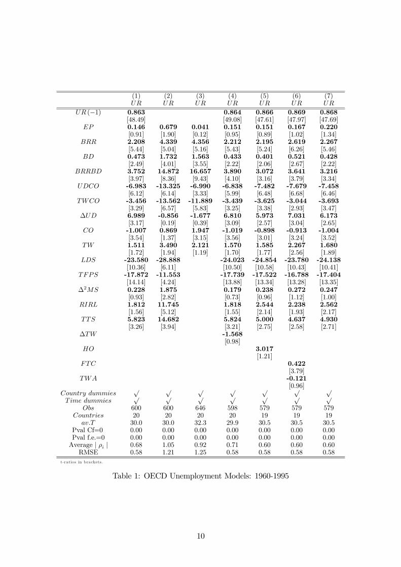
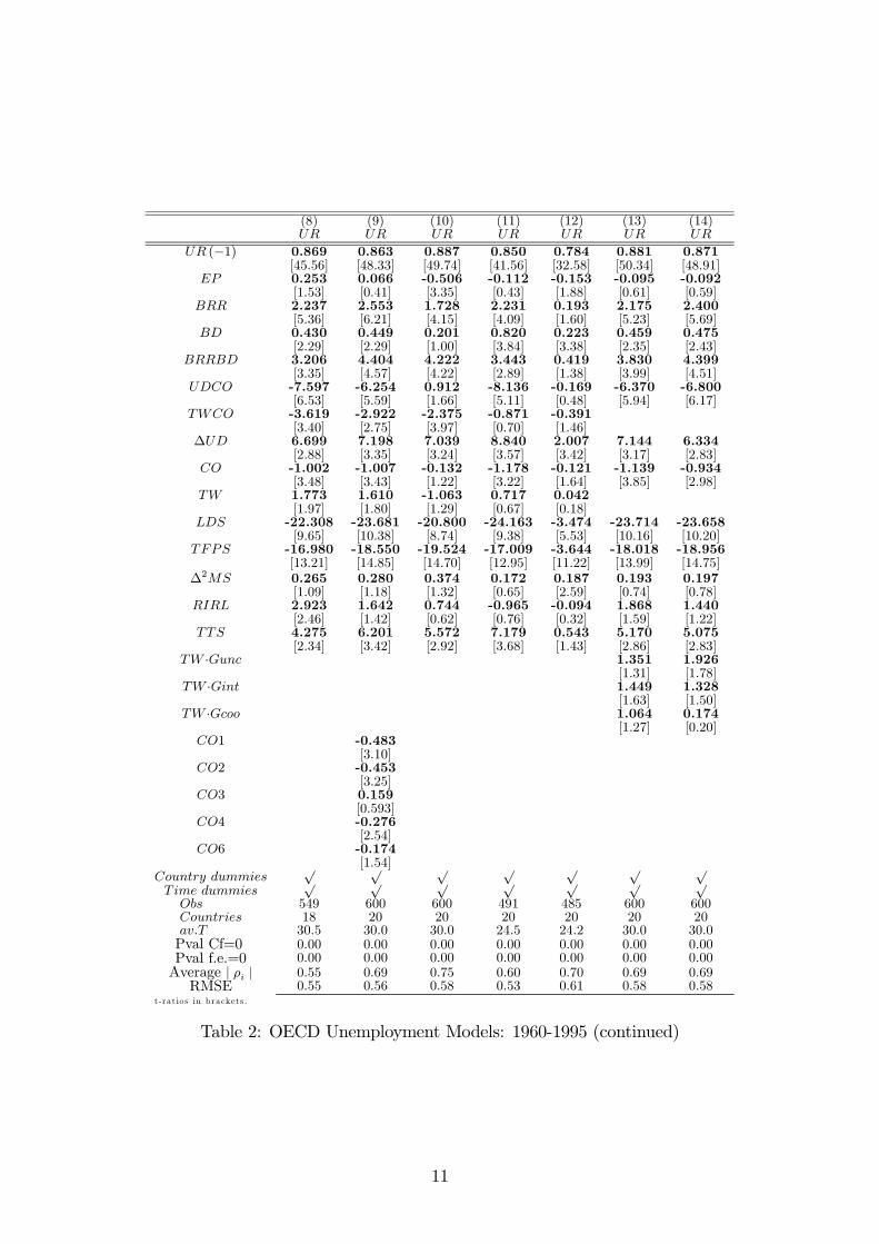
Tables 1, 2 and 3 present the estimation output from a set of alternative specifications of the
unemployment model of equation (1). These are:
1. the baseline model;
2. a static model;
3. a static model with no macroeconomic shocks;
4. a model including changes in the tax wedge, ∆TW ;
5. a model including Oswald’s Home Ownership variable12 (Portugal excluded) which rep-
resents the proportion of owner occupier households and is a proxy for labour mobility;
6. a model including an indicator of fixed term contracts and temporary work agencies
regulations (Portugal excluded);
7. a model excluding Portugal for a comparison with the previous model;
9See the argument contained in Nunziata (2001).10See Maddala and Wu (1996) and Fisher (1932).11The test relies on the assumption of no cross country correlation and whenever this assumption is not met
Maddala and Wu suggest bootstrapping to define the critical values. In our model we control for cross countrycorrelation by means of time dummies, and therefore we assume we are free to use the exact distribution ofthe test for inference.
12See Oswald (1996).
8

8. a model excluding Portugal and Spain in order to check for the impact of the non
democratic regimes in these countries in the 1970s and the transition to democracy
afterwards;
9. a model including coordination types dummies;
10. a model using an alternative measure of bargaining coordination;
11. a model estimated on a subsample from 1970;
12. a model estimated on a subsample from 1970, using unemployment in logs;
13. a model including a test of the hump shaped effect of taxation on unemployment, dividing
the countries into three groups according to their degree of bargaining coordination13;
14. a model including a second test of the hump shaped effect of taxation on unemploy-
ment, dividing the countries into three groups according to their degree of bargaining
centralization;
15. a model including union density in levels;
16. a model where macroeconomic shocks are substituted with the change in inflation;
17. the baseline model estimated by OLS;
18. the baseline model using 5 years averaged data;
19. the baseline model using 5 years averaged data, including union density in levels;
20. the baseline model using 5 years averaged data, including union density in levels and
Oswald’s Home Ownership variable.
All models are estimated by fixed effects GLS, with the correction for heteroskedasticity
and serial correlation commented on above, except for Model 17 which is estimated by OLS.
Model 1 is the benchmark specification. It is characterized by a significant effect for most
labour market institutions, except employment protection. Although the cointegration tests
13See Alesina and Perotti (1997) and Daveri and Tabellini (2000) for some empirical evidence on this.
9
(1) (2) (3) (4) (5) (6) (7)UR UR UR UR UR UR UR
UR (−1) 0.863 0.864 0.866 0.869 0.868
[48.49] [49.08] [47.61] [47.97] [47.69]EP 0.146 0.679 0.041 0.151 0.151 0.167 0.220
[0.91] [1.90] [0.12] [0.95] [0.89] [1.02] [1.34]BRR 2.208 4.339 4.356 2.212 2.195 2.619 2.267
[5.44] [5.04] [5.16] [5.43] [5.24] [6.26] [5.46]BD 0.473 1.732 1.563 0.433 0.401 0.521 0.428
[2.49] [4.01] [3.55] [2.22] [2.06] [2.67] [2.22]BRRBD 3.752 14.872 16.657 3.890 3.072 3.641 3.216
[3.97] [8.36] [9.43] [4.10] [3.16] [3.79] [3.34]UDCO -6.983 -13.325 -6.990 -6.838 -7.482 -7.679 -7.458
[6.12] [6.14] [3.33] [5.99] [6.48] [6.68] [6.46]TWCO -3.456 -13.562 -11.889 -3.439 -3.625 -3.044 -3.693
[3.29] [6.57] [5.83] [3.25] [3.38] [2.93] [3.47]∆UD 6.989 -0.856 -1.677 6.810 5.973 7.031 6.173
[3.17] [0.19] [0.39] [3.09] [2.57] [3.04] [2.65]CO -1.007 0.869 1.947 -1.019 -0.898 -0.913 -1.004
[3.54] [1.37] [3.15] [3.56] [3.01] [3.24] [3.52]TW 1.511 3.490 2.121 1.570 1.585 2.267 1.680
[1.72] [1.94] [1.19] [1.70] [1.77] [2.56] [1.89]LDS -23.580 -28.888 -24.023 -24.854 -23.780 -24.138
[10.36] [6.11] [10.50] [10.58] [10.43] [10.41]TFPS -17.872 -11.553 -17.739 -17.522 -16.788 -17.404
[14.14] [4.24] [13.88] [13.34] [13.28] [13.35]∆2MS 0.228 1.875 0.179 0.238 0.272 0.247
[0.93] [2.82] [0.73] [0.96] [1.12] [1.00]RIRL 1.812 11.745 1.818 2.544 2.238 2.562
[1.56] [5.12] [1.55] [2.14] [1.93] [2.17]TTS 5.823 14.682 5.824 5.000 4.637 4.930
[3.26] [3.94] [3.21] [2.75] [2.58] [2.71]∆TW -1.568
[0.98]HO 3.017
[1.21]FTC 0.422
[3.79]TWA -0.121
[0.96]Country dummies
√ √ √ √ √ √ √Time dummies
√ √ √ √ √ √ √Obs 600 600 646 598 579 579 579
Countries 20 20 20 20 19 19 19av.T 30.0 30.0 32.3 29.9 30.5 30.5 30.5
Pval Cf=0Pval f.e.=0
0.000.00
0.000.00
0.000.00
0.000.00
0.000.00
0.000.00
0.000.00
Average | ρi| 0.68 1.05 0.92 0.71 0.60 0.60 0.60
RMSE 0.58 1.21 1.25 0.58 0.58 0.58 0.58
t-ratios in brackets.
Table 1: OECD Unemployment Models: 1960-1995
10
(8) (9) (10) (11) (12) (13) (14)UR UR UR UR UR UR UR
UR (−1) 0.869 0.863 0.887 0.850 0.784 0.881 0.871
[45.56] [48.33] [49.74] [41.56] [32.58] [50.34] [48.91]EP 0.253 0.066 -0.506 -0.112 -0.153 -0.095 -0.092
[1.53] [0.41] [3.35] [0.43] [1.88] [0.61] [0.59]BRR 2.237 2.553 1.728 2.231 0.193 2.175 2.400
[5.36] [6.21] [4.15] [4.09] [1.60] [5.23] [5.69]BD 0.430 0.449 0.201 0.820 0.223 0.459 0.475
[2.29] [2.29] [1.00] [3.84] [3.38] [2.35] [2.43]BRRBD 3.206 4.404 4.222 3.443 0.419 3.830 4.399
[3.35] [4.57] [4.22] [2.89] [1.38] [3.99] [4.51]UDCO -7.597 -6.254 0.912 -8.136 -0.169 -6.370 -6.800
[6.53] [5.59] [1.66] [5.11] [0.48] [5.94] [6.17]TWCO -3.619 -2.922 -2.375 -0.871 -0.391
[3.40] [2.75] [3.97] [0.70] [1.46]∆UD 6.699 7.198 7.039 8.840 2.007 7.144 6.334
[2.88] [3.35] [3.24] [3.57] [3.42] [3.17] [2.83]CO -1.002 -1.007 -0.132 -1.178 -0.121 -1.139 -0.934
[3.48] [3.43] [1.22] [3.22] [1.64] [3.85] [2.98]TW 1.773 1.610 -1.063 0.717 0.042
[1.97] [1.80] [1.29] [0.67] [0.18]LDS -22.308 -23.681 -20.800 -24.163 -3.474 -23.714 -23.658
[9.65] [10.38] [8.74] [9.38] [5.53] [10.16] [10.20]TFPS -16.980 -18.550 -19.524 -17.009 -3.644 -18.018 -18.956
[13.21] [14.85] [14.70] [12.95] [11.22] [13.99] [14.75]∆2MS 0.265 0.280 0.374 0.172 0.187 0.193 0.197
[1.09] [1.18] [1.32] [0.65] [2.59] [0.74] [0.78]RIRL 2.923 1.642 0.744 -0.965 -0.094 1.868 1.440
[2.46] [1.42] [0.62] [0.76] [0.32] [1.59] [1.22]TTS 4.275 6.201 5.572 7.179 0.543 5.170 5.075
[2.34] [3.42] [2.92] [3.68] [1.43] [2.86] [2.83]TW ·Gunc 1.351 1.926
[1.31] [1.78]TW ·Gint 1.449 1.328
[1.63] [1.50]TW ·Gcoo 1.064 0.174
[1.27] [0.20]CO1 -0.483
[3.10]CO2 -0.453
[3.25]CO3 0.159
[0.593]CO4 -0.276
[2.54]CO6 -0.174
[1.54]Country dummies
√ √ √ √ √ √ √Time dummies
√ √ √ √ √ √ √ObsCountriesav.T
5491830.5
6002030.0
6002030.0
4912024.5
4852024.2
6002030.0
6002030.0
Pval Cf=0Pval f.e.=0
0.000.00
0.000.00
0.000.00
0.000.00
0.000.00
0.000.00
0.000.00
Average | ρi|
RMSE0.550.55
0.690.56
0.750.58
0.600.53
0.700.61
0.690.58
0.690.58
t-ratios in brackets.
Table 2: OECD Unemployment Models: 1960-1995 (continued)
11

(15) (16) (17) (18) (19) (20)UR UR UR UR UR UR
UR (−1) 0.859 0.876 0.867
[47.16] [41.81] [42.27]EP 0.257 -0.053 -0.254 0.935 0.966 0.955
[1.47] [0.34] [0.95] [2.45] [2.54] [2.08]BRR 2.457 1.977 2.783 3.123 3.068 3.846
[6.05] [4.87] [5.17] [2.59] [2.85] [3.40]BD 0.560 0.006 0.335 2.496 2.794 3.228
[2.84] [0.04] [1.07] [3.65] [3.99] [4.42]BRRBD 4.067 3.952 4.316 5.731 5.841 7.607
[4.31] [4.16] [3.36] [2.57] [2.72] [3.35]UDCO -7.224 -3.679 -4.472 -15.655 -14.925 -14.527
[6.01] [3.15] [2.87] [5.57] [5.22] [4.79]TWCO -3.620 -1.748 -1.836 -15.788 -16.132 -17.160
[3.40] [1.61] [1.27] [4.92] [5.53] [5.79]∆UD 7.138 4.247 1.028
[3.16] [1.64] [0.10]CO -0.947 -0.492 -0.958 0.212 0.210 0.126
[3.38] [1.60] [2.98] [0.29] [0.31] [0.18]TW 1.488 1.839 2.224 1.491 1.839 1.272
[1.70] [2.00] [1.93] [0.66] [0.85] [0.57]LDS -25.903 -22.847 -86.342 -85.754 -84.199
[11.18] [8.80] [8.37] [8.51] [7.45]TFPS -18.257 -20.422 -26.515 -32.340 -33.949
[14.24] [12.41] [3.05] [3.27] [2.77]∆2MS 0.385 0.456 12.731 12.762 14.586
[1.48] [1.72] [2.38] [2.62] [2.48]RIRL 1.505 0.713 27.528 29.244 31.334
[1.28] [0.52] [4.82] [5.62] [5.22]TTS 5.927 5.782 79.703 78.062 73.510
[3.32] [2.87] [10.75] [10.59] [9.23]UD -0.224 2.581 2.049
[0.24] [1.38] [1.04]HO -1.517
[0.29]∆2p -0.170
[4.10]Country dummies
√ √ √ √ √ √Time dummies
√ √ √ √ √ √Obs 600 636 600 127 127 123
Countries 20 20 20 20 20 19av.T 30.0 31.8 30.0 30.0 30.0 30.0
Pval Cf=0Pval f.e.=0
0.000.00
0.000.00
0.000.00
0.000.00
0.000.00
0.000.00
Average | ρi| 0.70 0.68 0.57
RMSE 0.58 0.58 0.69 0.56 0.62 0.62
t-ratios in brackets.
Table 3: OECD Unemployment Models: 1960-1995 (continued)
12

Time dummies
1966 0.07 (0.3) 1976 0.69 (0.6) 1986 0.62 (0.3)1967 0.02 (0.1) 1977 0.61 (0.5) 1987 0.79 (0.4)1968 0.11 (0.3) 1978 0.72 (0.5) 1988 0.56 (0.3)1969 -0.06 (0.1) 1979 0.59 (0.4) 1989 0.53 (0.2)1970 0.11 (0.2) 1980 0.55 (0.4) 1990 0.98 (0.4)1971 0.37 (0.6) 1981 1.14 (0.7) 1991 1.33 (0.5)1972 0.5 (0.7) 1982 1.41 (0.8) 1992 1.62 (0.6)1973 0.28 (0.3) 1983 1.21 (0.7) 1993 1.55 (0.6)1974 0.08 (0.1) 1984 0.69 (0.4) 1994 1.14 (0.4)1975 0.92 (0.9) 1985 0.52 (0.3) 1995 0.58 (0.2)
t-ratios in brackets.
Table 4: Time dummies from model (1)
Time Trends
Australia -0.054 (0.5) Japan -0.059 (0.6)Austria -0.059 (0.6) Netherlands -0.045 (0.5)Belgium -0.022 (0.2) Norway -0.067 (0.7)Canada -0.072 (0.8) New Zealand 0.003 (0.0)
Denmark -0.078 (0.8) Portugal -0.107 (1.1)Finland 0.017 (0.2) Spain 0.042 (0.4)France -0.019 (0.2) Sweden -0.078 (0.8)
Germany -0.006 (0.1) Switzerland -0.041 (0.4)Ireland 0.022 (0.2) UK -0.007 (0.1)
Italy -0.015 (0.2) US -0.026 (0.3)
t-ratios in brackets.
Table 5: Time trends from model (1)
13
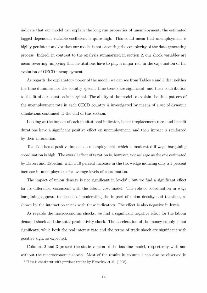
indicate that our model can explain the long run properties of unemployment, the estimated
lagged dependent variable coefficient is quite high. This could mean that unemployment is
highly persistent and/or that our model is not capturing the complexity of the data generating
process. Indeed, in contrast to the analysis summarized in section 2, our shock variables are
mean reverting, implying that institutions have to play a major role in the explanation of the
evolution of OECD unemployment.
As regards the explanatory power of the model, we can see from Tables 4 and 5 that neither
the time dummies nor the country specific time trends are significant, and their contribution
to the fit of our equation is marginal. The ability of the model to explain the time pattern of
the unemployment rate in each OECD country is investigated by means of a set of dynamic
simulations contained at the end of this section.
Looking at the impact of each institutional indicator, benefit replacement rates and benefit
durations have a significant positive effect on unemployment, and their impact is reinforced
by their interaction.
Taxation has a positive impact on unemployment, which is moderated if wage bargaining
coordination is high. The overall effect of taxation is, however, not as large as the one estimated
by Daveri and Tabellini, with a 10 percent increase in the tax wedge inducing only a 1 percent
increase in unemployment for average levels of coordination.
The impact of union density is not significant in levels14, but we find a significant effect
for its difference, consistent with the labour cost model. The role of coordination in wage
bargaining appears to be one of moderating the impact of union density and taxation, as
shown by the interaction terms with these indicators. The effect is also negative in levels.
As regards the macroeconomic shocks, we find a significant negative effect for the labour
demand shock and the total productivity shock. The acceleration of the money supply is not
significant, while both the real interest rate and the terms of trade shock are significant with
positive sign, as expected.
Columns 2 and 3 present the static version of the baseline model, respectively with and
without the macroeconomic shocks. Most of the results in column 1 can also be observed in
14This is consistent with previous results by Elmeskov et al. (1998).
14

column 2, except that there is now a significant positive effect for employment protection, but
no effect from the change in union density, and coordination in levels. Column 3 indicates,
instead, that once we omit the controls for macro shocks, the model produces inconsistent
results, especially regarding the tax wedge and the coordination indicators. This result sug-
gests that the macro controls are needed in order to obtain a clean estimate of the long run
relationship between unemployment and institutions.
In column 4 we check for a rate of change effect in the tax wedge, which is not found
significant. Column 5 indicates a positive although weak impact of home ownership15. Column
6 shows that strict fixed term contract regulations have a positive impact on unemployment,
while temporary agency regulations are not significant. This result is consistent with the
empirical findings of Nunziata and Staffolani (2003) on a sample of ten European countries.
The last two models are estimated excluding Portugal because no data are available on
these indicators for that country. We check, therefore, the effect of omitting Portugal in
column 7, and of omitting both Portugal and Spain in column 8. This is also to ensure that
the inclusion of two countries characterized by non democratic regimes up to the mid 1970s
does not affect our estimates. The main results are very stable, and all our findings are
confirmed if not reinforced.
Model 9 includes a set of coordination dummies proposed by Traxler and Kittel16 that
describe the type of coordination which is prevalent in each country at any time. These are:
CO1=inter-associational coordination, i.e. coordination by the major confederations of
employers and labour;
CO2=intra-associational coordination, i.e. within the major confederations of employers
and labour;
CO3=pattern setting coordination, i.e. actions by a dominant sector establishing a pattern
for other sectors;
CO4=state imposed coordination;
15As we will see below, the high interpolation of this institutional indicator does not seem to be enough toaccount for this explanatory weakness.
16See Traxler (1996) and Traxler and Kittel (2000). We include five of the six categorical variables originallyset by these authors, excluding CO5, non-coordination, in order to avoid multicollinearity.
15
CO6=state sponsored coordination, i.e. with the state joining the bargaining process as
an additional party.
The coordination types that have a significant and negative effect on unemployment are
inter-associational, intra-associational and state imposed coordination.
In model 10 we check the robustness of the coordination effect using an alternative indicator
provided by Nickell et al. (2002) that accounts for short term variation in coordination. The
effect, in levels, of coordination, as well as the effect of the interaction with union density,
disappear. However, the interaction with the tax wedge is robust to the change in the indicator,
remaining negative and significant.
Model 11 is the baseline equation estimated from 1970 onwards. After dropping almost 20
percent of the observations, most of the institutional effects are confirmed, although the tax
wedge effect is not significant both in levels and interacted with coordination. If we estimate
the model over the same period but using unemployment in logs17, as in column 12, the effect
of institutions appears to be moderately weaker.
Columns 13 and 14 present a test of the Alesina and Perotti and Daveri and Tabellini
hypothesis18 of a hump shaped effect of taxation on unemployment. In the first case we divide
the observations into three groups according to the degree of wage bargaining coordination.
Each group is defined, respectively, as uncoordinated, intermediate and highly coordinated.
We then construct a dummy for each group and interact it with the tax wedge indicator. The
numerical criteria defining each group are the same as in the wage equation19. The tax wedge
effect is only vaguely hump shaped in model 13, with a 10% level significant positive effect on
intermediate countries only. If we substitute our coordination measure with a centralization
indicator, as in column 14, we find instead a positive significant impact in countries with
decentralized bargaining only. In addition, the tax effect is weaker the higher is centralization.
Model 15 contains the union density indicator in levels, which is found to be insignificant.
Model 16 substitutes the macroeconomic shock controls with an inflation change variable
17Using logs of unemployment from 1970 onwards is not problematic (as it is in the full sample case) sincesome countries are characterized by unemployment rates close to zero in the early 1960s only.
18See Alesina and Perotti (1997) and Daveri and Tabellini (2000).19Gunc is the dummy for the group of uncoordinated countries, characterized by a coordination level CO <
1.5. Gint is the indicator for the intermediate countries, with 1.5 ≤ CO ≤ 2, and Gcoo is the indicator forhighly coordinated countries with CO > 2.
16

in order to replicate the results of previous models, such as Nickell (1997). The variable’s
coefficient is negative and significant and the institutional coefficients are robust to this change,
apart from that on the benefit durations indicator, which becomes insignificant.
The OLS estimation of the baseline model, i.e. without taking into account the problems of
heteroskedasticity and serial correlation, is presented in column 17. The estimates of columns
1 and 17 are very similar, apart from the lack of significance of the benefit duration indicator.
Another robustness check is presented in the last three columns of Table 3. These models
are estimated using five years averaged data, reducing the number of observations from 600
to 127. The 5 years averaged version of the baseline model, presented in column 18, confirms
most of our previous results, apart from the lack of significance of the tax wedge in levels and
the rate of change in union density. Model 19 includes union density in levels which has a
weak positive effect. The home ownership variable effect is estimated in model 20. Although
the 5 years averaging reduces the degree of interpolation in the home ownership indicator, the
coefficient is still not statistically significant.
Summarizing the results above, our models are able to produce a quite satisfactory expla-
nation of the unemployment patterns in OECD countries. The empirical results are largely
consistent with the findings of a similar analysis of OECD labour costs presented in Nunziata
(2001). It is possible that with better institutional indicators on unions and with information
on the enforcement of the unemployment benefits we would be able to produce better results
that do not have to rely on such a high level of endogenous persistence to fit the data.
The next section contains a set of dynamic simulations of the baseline model in order
to assess how much of the unemployment evolution in each country can be explained by
institutions.
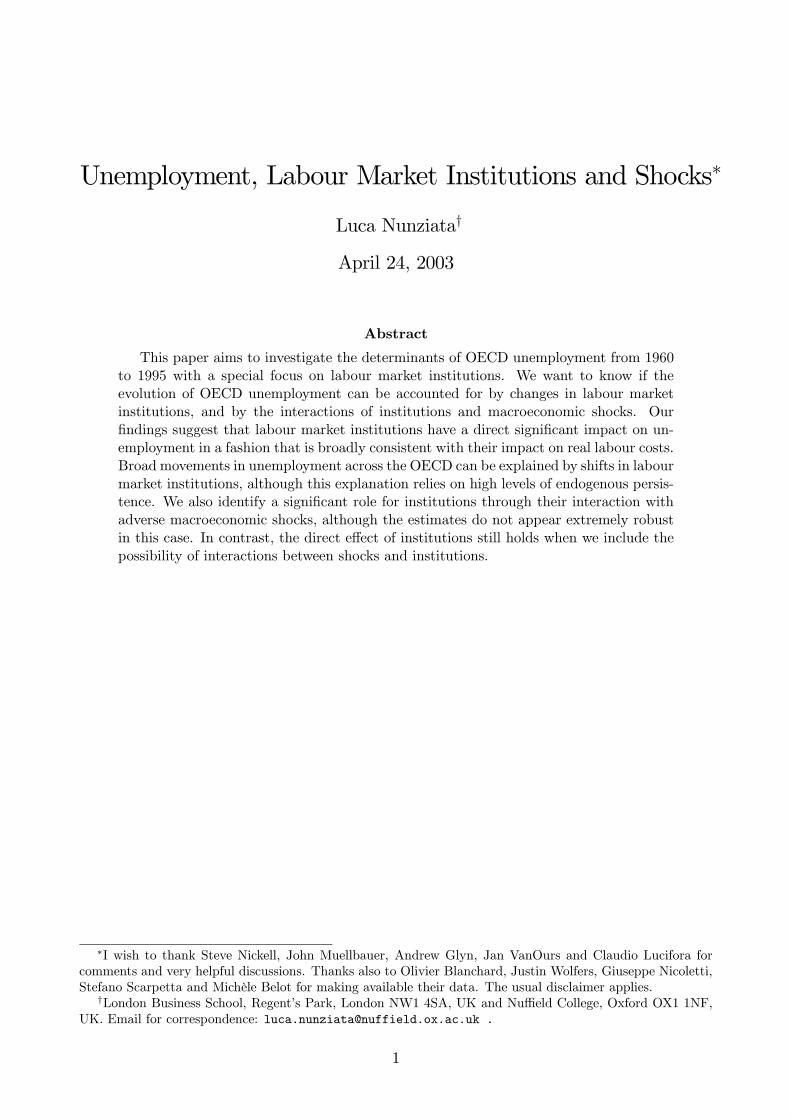
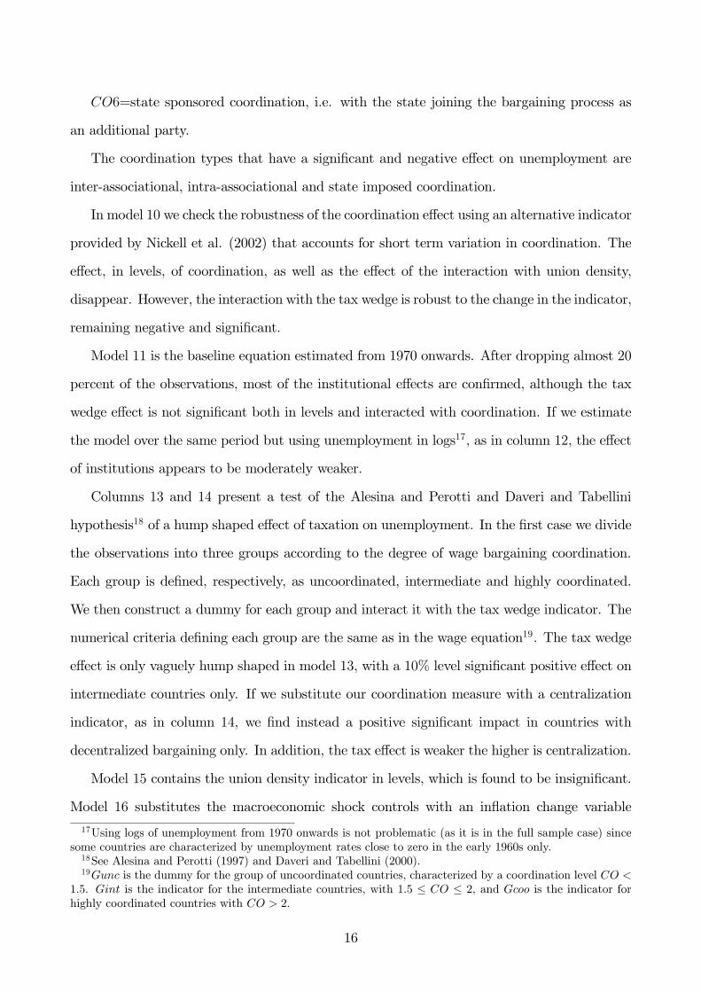
2.4 Dynamic Simulations
The model simulations generate an unemployment series for each country through a recursive
procedure that substitutes the lagged dependent variable with the previous year’s predicted
value obtained from the baseline model20. Figure 1 displays actual unemployment and the
20This is the same procedure employed in Nunziata (2001).
17
Une
mpl
oym
ent R
ate
Year
Actual unemployment rate Standard dynamic simulation
Australia
1970 1975 1980 1985
2468
10
Austria
1960 1970 1980 19902000
1
2
3
4
Belgium
1960 1970 1980 199020000
5
10
15
Canada
1960 1970 1980 199020000
5
10
15
Denmark
1960 1970 1980 199020000
5
10
Finland
1960 1970 1980 1990200005
101520
France
1960 1970 1980 199020000
5
10
15
Germany
1960 1970 1980 1990200002468
Ireland
1960 1970 1980 1990200005
101520
Italy
1960 1970 1980 199020002468
10
Japan
1960 1970 1980 19902000-20246
Netherlands
1960 1970 1980 199020000
5
10
15
Norway
1960 1970 1980 199020000
2
4
6
New Zealand
1975 1980 19850
2
4
6
Portugal
1975 1980 1985 199019954
6
8
10
Spain
1960 1970 1980 199020000
10
20
30
Sweden
1960 1970 1980 199020000
5
10
Switzerland
1960 1970 1980 19902000-2
0
2
4
United Kingdom
1960 1970 1980 199020000
5
10
15
United States
1960 1970 1980 199020002468
10
Figure 1: The unemployment model fit: actual and simulated unemployment
Une
mpl
oym
ent R
ate
Year
Standard dynamic simulation All institutions fixed
Australia
1970 1975 1980 1985
2468
10
Austria
1960 1970 1980 19902000
-4-2024
Belgium
1960 1970 1980 199020000
5
10
15
Canada
1960 1970 1980 19902000-5
0
5
10
Denmark
1960 1970 1980 19902000-5
0
5
10
Finland
1960 1970 1980 199020000
5
10
15
France
1960 1970 1980 199020000
5
10
15
Germany
1960 1970 1980 1990200002468
Ireland
1960 1970 1980 1990200005
101520
Italy
1960 1970 1980 199020000
5
10
Japan
1960 1970 1980 19902000
-20246
Netherlands
1960 1970 1980 199020000
5
10
Norway
1960 1970 1980 19902000-20246
New Zealand
1975 1980 19850
2
4
6
Portugal
1975 1980 1985 19901995-5
0
5
10
Spain
1960 1970 1980 199020000
10
20
30
Sweden
1960 1970 1980 19902000
-5
0
5
10
Switzerland
1960 1970 1980 19902000-4-2024
United Kingdom
1960 1970 1980 199020000
5
10
15
United States
1960 1970 1980 19902000
4
6
8
10
Figure 2: Dynamic simulations keeping all isntitutions fixed at average 1960s values
18

Une
mpl
oym
ent R
ate
chan
ge
-4
-2
0
2
4
6
8
10
Unemployment Benefits Tax Wedge Coordination Union Density Employment Protection Real Interest Rate
ALAU
BECA
DKFN
FRGE
IRIT
JANL
NWNZ
PGSP
SWSZ
UKUS
Figure 3: Dynamic simulations with regressors fixed at 1960s average values: changes inunemployment in the 1980s imputed to specific institutional dimensions
Une
mpl
oym
ent R
ate
chan
ge
-8
-4
0
4
8
12
16
Unemployment Benefits Tax Wedge Coordination Union Density Employment Protection Real Interest Rate
ALAU
BECA
DKFN
FRGE
IRIT
JANL
NWNZ
PGSP
SWSZ
UKUS
Figure 4: Dynamic simulations with regressors fixed at 1960s average values: changes inunemployment in the 1990s imputed to specific institutional dimensions
19

simulated series for each country, showing a good overall fit for each country, apart from
Portugal and, to a lesser extent, Japan.
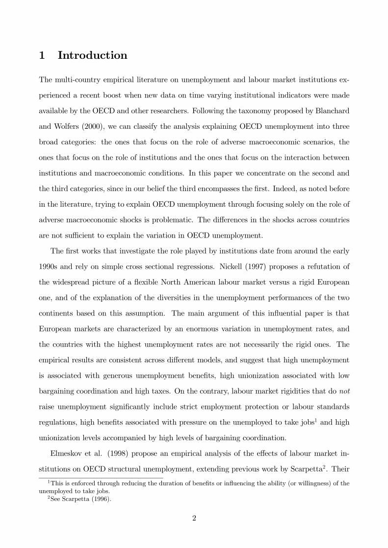
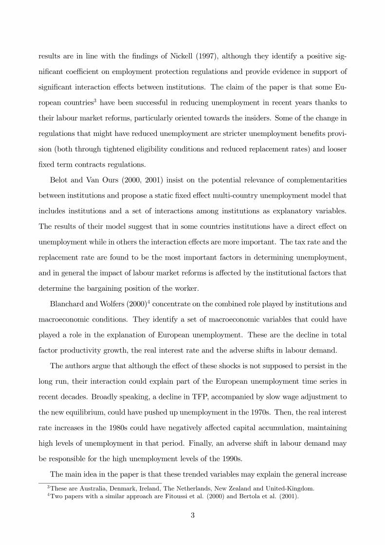
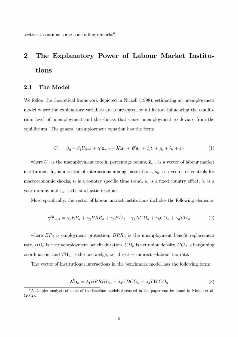
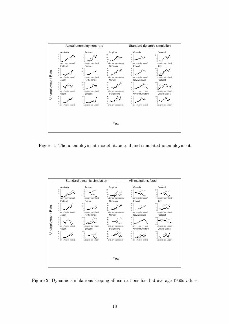
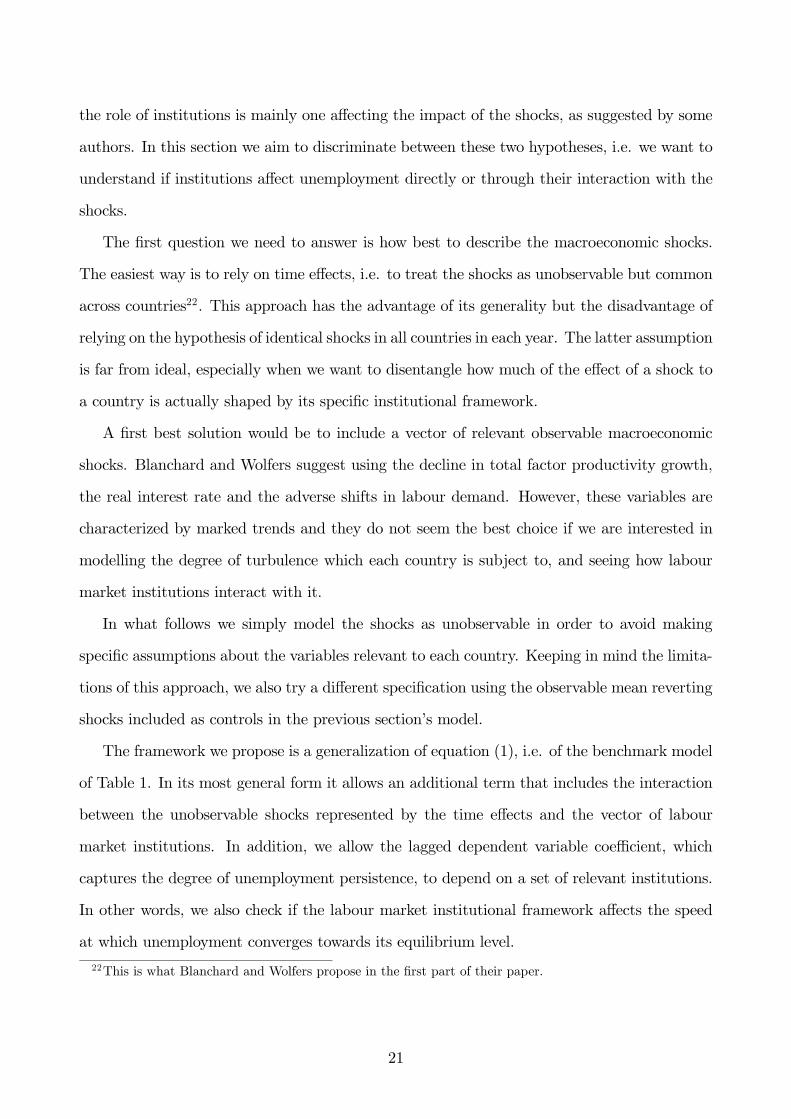
A summary account of the dynamic simulations is contained in Figures 3 and 4, where the
impact of each institution is assessed in a comparative way. We constrain each regressor at its
average 1960s value and the impact of each institutional dimension is stacked on each country
bar. In this way we calculate the variation in unemployment that can be attributed to the
evolution of specific regressors over the estimation period.
Overall, the institutions seem to explain a significant part of the change in unemploy-
ment since the 1960s in Australia, Belgium, Denmark, Finland, France, Italy, Netherlands,
Norway, Spain, Switzerland and the UK. They probably explain too much in Austria, Portu-
gal and Sweden, while they are unsuccessful in explaining unemployment in Germany, New
Zealand and the US. The last case is not a surprise given the mainly cyclical nature of US
unemployment.
Looking at the simulation figures we notice that the labour market institutions can explain
around 55 percent of the 6.8 percent increase in the average European unemployment rate from
the 1960s to the 1990s21. The model’s explanatory power is therefore very good, especially
considering the fact that the early 1990s were characterized by a deep recession in most
European countries. If we exclude Germany from this calculation, a country for which our
model is not able to say much, we explain 63 percent of the rise in unemployment in the rest
of Europe.
The combination of benefits and taxes are responsible for two-thirds of that part of the
long-term rise in European unemployment that our institutions explain.
3 Institutions and Shocks: a General Framework
In the previous section we proposed a model whose explanation of the evolution of unemploy-
ment in OECD countries is based on the direct effect of institutions, controlling for a set of
mean reverting macroeconomic shocks. What we have not examined is the hypothesis that
21Note that we consider European OECD countries only, therefore excluding Greece and Eastern Europe.
20
the role of institutions is mainly one affecting the impact of the shocks, as suggested by some
authors. In this section we aim to discriminate between these two hypotheses, i.e. we want to
understand if institutions affect unemployment directly or through their interaction with the
shocks.
The first question we need to answer is how best to describe the macroeconomic shocks.
The easiest way is to rely on time effects, i.e. to treat the shocks as unobservable but common
across countries22. This approach has the advantage of its generality but the disadvantage of
relying on the hypothesis of identical shocks in all countries in each year. The latter assumption
is far from ideal, especially when we want to disentangle how much of the effect of a shock to
a country is actually shaped by its specific institutional framework.
A first best solution would be to include a vector of relevant observable macroeconomic
shocks. Blanchard and Wolfers suggest using the decline in total factor productivity growth,
the real interest rate and the adverse shifts in labour demand. However, these variables are
characterized by marked trends and they do not seem the best choice if we are interested in
modelling the degree of turbulence which each country is subject to, and seeing how labour
market institutions interact with it.
In what follows we simply model the shocks as unobservable in order to avoid making
specific assumptions about the variables relevant to each country. Keeping in mind the limita-
tions of this approach, we also try a different specification using the observable mean reverting
shocks included as controls in the previous section’s model.
The framework we propose is a generalization of equation (1), i.e. of the benchmark model
of Table 1. In its most general form it allows an additional term that includes the interaction
between the unobservable shocks represented by the time effects and the vector of labour
market institutions. In addition, we allow the lagged dependent variable coefficient, which
captures the degree of unemployment persistence, to depend on a set of relevant institutions.
In other words, we also check if the labour market institutional framework affects the speed
at which unemployment converges towards its equilibrium level.
22This is what Blanchard and Wolfers propose in the first part of their paper.
21

In analytical terms, the model in equation (1) is generalized as follows:
Uit = β0+ β
1tUit−1 + γ′
1z1w,it + λ′
hit + ϑ′sit + φiti + µi + λt
(1 + γ′
2zd2w,it
)+ εit (5)
where β1t =
(α0 + γ ′
3zd3w,it
), and the superscript d stands for deviation from the world
average.
Equation (5) suggests that institutions may have three distinct roles in explaining OECD
unemployment:
1. they may directly affect unemployment as in model (1) through the vectors γ′
1z1w,it and
λ′hit;
2. they may shape the impact of the shocks through the interaction with the time effects
λt
(1 + γ ′
2zd2w,it
);
3. they may affect unemployment persistence through the lagged dependent variable coef-
ficient β1t =
(α0 + γ′
3zd3w,it
).
Note that the two vectors of interacted institutions zd2w,it and z
d3w,it are expressed as devi-
ations from the world average so that we may interpret the coefficients on the institutions in
levels as the coefficients of the average country.
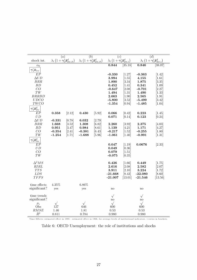
The results of our estimations are presented in Tables 6, 7 and 8. They include, in addition
to the general model of equation (5), a range of alternative specifications in order to check the
robustness of our findings23.
We first try to replicate Blanchard and Wolfers’ results estimating an analogous model, i.e.
regressing unemployment on a constant, the country dummies and the time effects interacted
with institutions:
Uit = β0+ µi + λt (1 + γ′
2z2w,it) + εit . (6)
23In order to avoid confusion with the previous section, we denote each model in this section with a letterinstead of a number.
22

Their sample of countries and the time period is the same as ours, although they use 5 years
averaged data instead of annual data. Model a is the replica of their model on our (averaged)
data. Our specification differ from theirs because we end up having 127 observations instead of
15924, and because our institutional indicators are all time varying25. In column b we estimate
the same model on annual data. Both models include union density in delta form since we do
not find a significant effect for the level.
Our results in column a are broadly in line with the findings of Blanchard and Wolfers.
Each institution enters significantly with the expected sign with the exception of union density,
which is not significant, and the tax wedge which has a negative coefficient. The fit of the
equation is also comparable, with an R2 equal to 0.811 instead of 0.863. These results are
confirmed when we use annual data as in column b, with the addition of a significant effect
of union density in delta form and a slightly worse fit. The time effects are significant in
each model and they account, respectively, for a 4.35% and a 6.86% rise in unemployment
for average values of all institutional indicators26. This is less than the 7.3% estimated by
Blanchard and Wolfers.
This simple specification offers a good description of the data. The task now is to assess
whether what matters more in explaining OECD unemployment is the direct role of institu-
tional changes, or the role of the interactions between institutions and shocks. Columns c to n
in the tables present a set of alternative specifications of equation (5) in order to discriminate
between these two hypotheses. Following Blanchard and Wolfers we first present a simpler
version of the model interacting both the LDV and the time effects with a set of time invariant
institutional indicators27. We then proceed to use the time varying indicators.
Model c is estimated using time invariant indicators in the interactions. Among the in-
teracted institutions only, the benefit indicators are significant with expected sign, and most
of the results of section 3 are confirmed. In addition, the time effects are not significant. If
24The reason for the limited sample is twofold: we have 7 observations per country while Blanchard andWolfers have 8, and our panel is unbalanced. Some of the regressors are not available for some years, in someof the countries.
25Blanchard and Wolfers present a version of their model including time varying indicators for the benefitreplacement rates and employment protection only.
26The impact of the time effects is calculated as estimated time effect in 1995 minus estimated time effectin the first available year.
27These are calculated as country averages of each indicator over the sample.
23

we reduce the model, and interact the lagged dependent variable with employment protection
only, as in column d, we also find that the latter is significant with the expected positive sign.
In other words, stricter employment protection increases unemployment persistence.
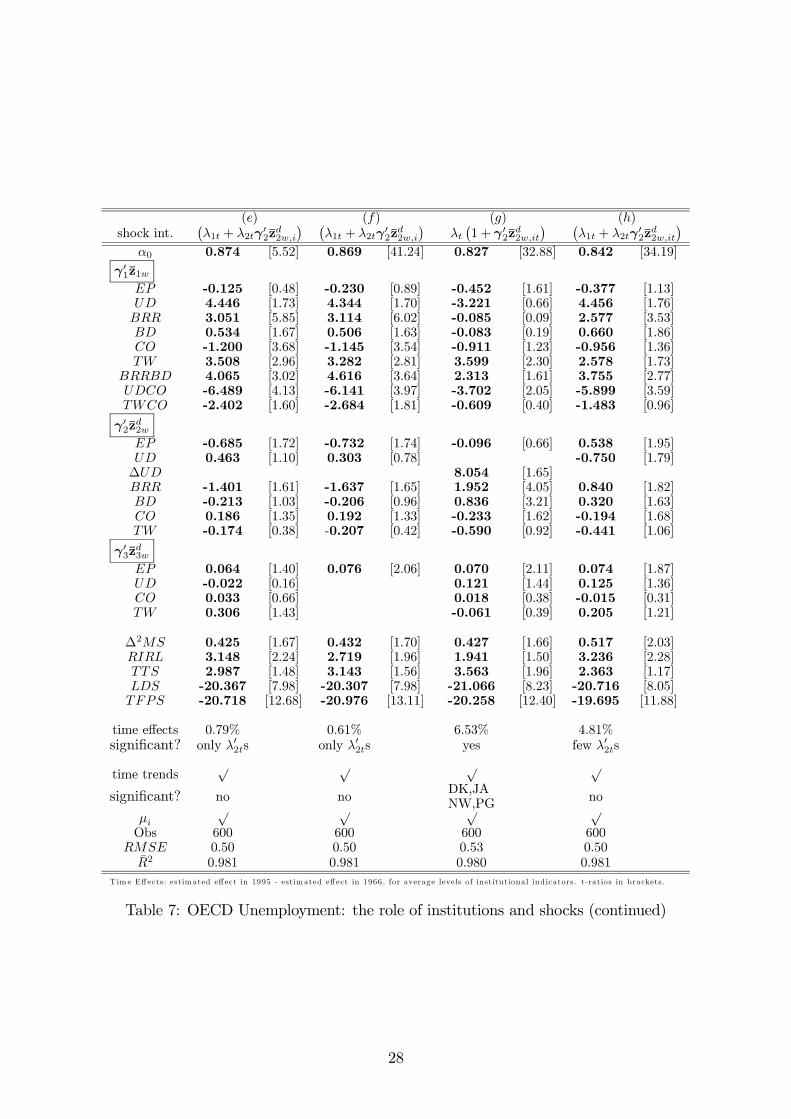
The characterization of the interactions between institutions and shocks adopted in columns
c and d is the same as Blanchard and Wolfers’, i.e. λt
(1 + γ′
2zd2w,it
). This specification im-
plicitly assumes that each shock is shaped by institutions in the same fashion at any time.
Models e and f relax this assumption, allowing the effect of each time dummy to depend dif-
ferently on the interacted institutions in each year. In analytical terms, we use a more general
specification such as(λ1t + λ2tγ
′
2zd2w,it
)that accounts for a partition of the effect of each shock
into two bits, one interacted with institutions and one not. Every year, a different fraction
of the shock will impact unemployment through its interaction with institutions. In this way
we control for the possibility that the interactions may have a different degree of importance
when a country faces shocks of different nature.
The estimation results of columns e and f provide a further, even more impressive, confir-
mation of the direct effect of institutions analysed in section 3. As regards the interactions,
most institutions are not significant, with the exception of employment protection which has
a negative coefficient28. Again, however, the time effects are not significant, and in model f
stricter employment protection reduces the adjustment speed of unemployment.
Blanchard and Wolfers typically obtain weaker results when interacting the shocks with
time varying institutions. This is not necessarily true in our case. Models g and h use time
varying institutional indicators in the interactions. They include, respectively, the simple and
the more general characterization of the interactions depicted above.
Model g is the only specification where the interacted institutions seem to play a more
important role than the institutions in levels. The tax wedge and the interaction between
coordination and union density are the only variables that show up in levels rather than as
interactions. The time effects are significant, and they account for a 6.53% rise in unemploy-
ment at average values of all institutions. The significant impact of employment protection
on unemployment persistence is confirmed.
28These results are confirmed when we drop the controls for the mean reverting macro shocks ϑ′sit.
24

When we adopt the more general specification for the interactions, as in column h, these
results are partially reversed. The institutions in levels are now significant with expected
sign, with the only exception being a weak effect from coordination29. In addition, we find
several significant interacted effects and again a significant impact of employment protection
on unemployment persistence. The time effects account for a 4.81% rise in unemployment at
average institutional levels. In contrast to the previous results, the coefficient on interacted
union density is negative.
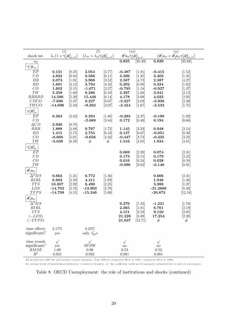
The specifications in columns i and l are the same as the ones in columns g and h, but
without including the lagged dependent variable. In these columns, both institutions in levels
and interacted are significant with expected sign, except for coordination in levels and the
interacted tax wedge in column i. In addition, the time effects can explain a rise in unem-
ployment equal, respectively, to 2.17% and 8.23%. Employment protection is now significant
in levels in column l.
Finally, modelsm and n provide an attempt to substitute the interactions with time effects
with a set of observable shocks. The variables we use are the ones contained in the vector
sit, i.e. a labour demand shock, a total factor productivity shock, a money supply shock, the
long term interest rate, and a terms of trade shock30. Each variable in the new vector sit is
constructed in order to be an adverse shock31. The main difference compared to variables used
by Blanchard and Wolfers is the fact that our shocks are mean reverting.
As with the time effects, we provide two alternative specifications for the interactions be-
tween institutions and shocks. Model m contains a simple interaction of the form ϑ′sitγ
′
2z2w,it
as in Blanchard and Wolfers, while model n contains a more general specification of the form
(ϑ′
1sit + ϑ′
2sitγ
′
2z2w,it). Both models contain non-interacted time dummies as controls. These
do not yield significant coefficients.
The estimation results show a significant effect of expected sign for interacted coordination
and benefit replacement rates, and this is common to both models. As regards the institutions
in levels, the tax wedge and the benefit replacement rates are significant in both specifications,
29Note that employment protection was also insignificant in Table 1.30See the definition of each shock on page 6.31This means that ϑ′
sit = θ1LDS∗
it+θ2TFPSH∗
it+θ3D2MSit+θ4RIRLit+θ5TTSit, with LDS∗
it=−LDSit
and TFPSH∗
it=−TFPSHit .
25
Une
mpl
oym
ent R
ate
Year
Standard dynamic simulation With shocks constant
Australia
1970 1975 1980 19850
5
10
Austria
1960 1970 1980 199020000
2
4
Belgium
1960 1970 1980 199020000
5
10
Canada
1960 1970 1980 19902000
468
1012
Denmark
1960 1970 1980 199020000
5
10
Finland
1960 1970 1980 199020000
5
10
15
France
1960 1970 1980 199020000
5
10
15
Germany
1960 1970 1980 1990200002468
Ireland
1960 1970 1980 199020000
5
10
15
Italy
1960 1970 1980 199020002468
10
Japan
1960 1970 1980 1990200001234
Netherlands
1960 1970 1980 199020000
5
10
Norway
1960 1970 1980 199020000
2
4
6
New Zealand
1975 1980 19850
2
4
6
Portugal
1975 1980 1985 199019952468
10
Spain
1960 1970 1980 199020000
10
20
30
Sweden
1960 1970 1980 199020000
5
10
Switzerland
1960 1970 1980 19902000-2
0
2
4
United Kingdom
1960 1970 1980 199020000
5
10
15
United States
1960 1970 1980 19902000
4
6
8
10
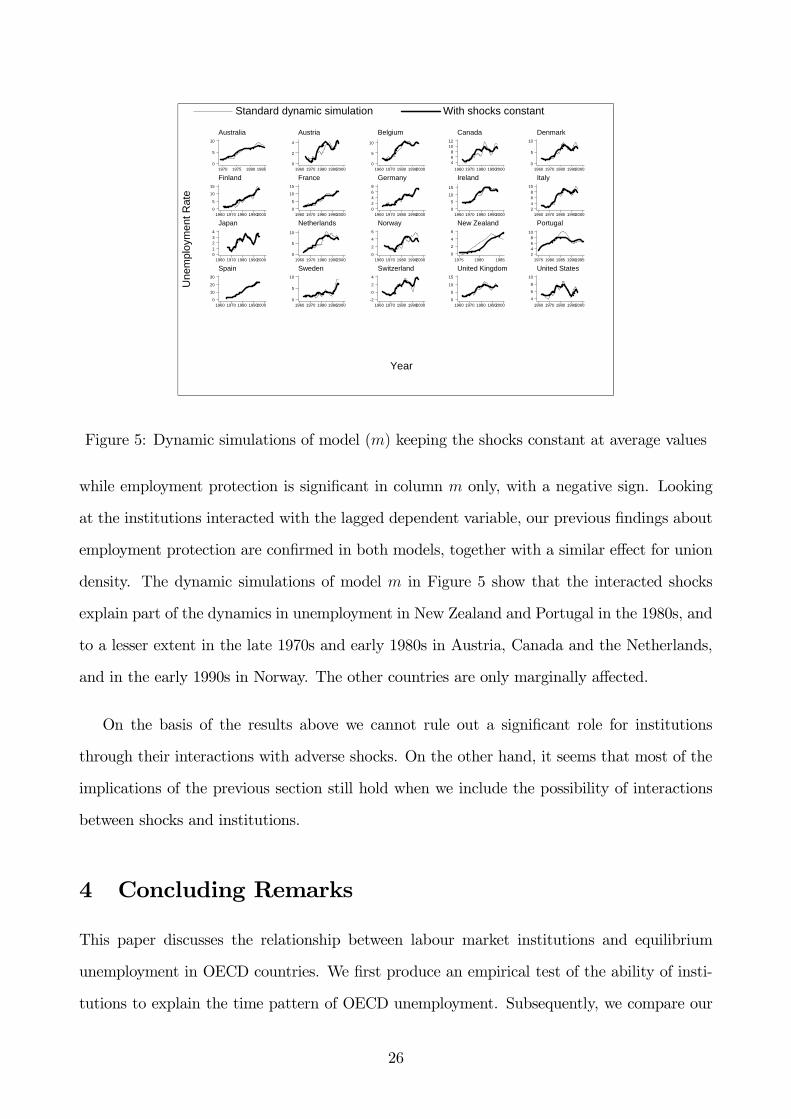
Figure 5: Dynamic simulations of model (m) keeping the shocks constant at average values
while employment protection is significant in column m only, with a negative sign. Looking
at the institutions interacted with the lagged dependent variable, our previous findings about
employment protection are confirmed in both models, together with a similar effect for union
density. The dynamic simulations of model m in Figure 5 show that the interacted shocks
explain part of the dynamics in unemployment in New Zealand and Portugal in the 1980s, and
to a lesser extent in the late 1970s and early 1980s in Austria, Canada and the Netherlands,
and in the early 1990s in Norway. The other countries are only marginally affected.
On the basis of the results above we cannot rule out a significant role for institutions
through their interactions with adverse shocks. On the other hand, it seems that most of the
implications of the previous section still hold when we include the possibility of interactions
between shocks and institutions.
4 Concluding Remarks
This paper discusses the relationship between labour market institutions and equilibrium
unemployment in OECD countries. We first produce an empirical test of the ability of insti-
tutions to explain the time pattern of OECD unemployment. Subsequently, we compare our
26
(a) (b) (c) (d)shock int. λt
(1 + γ′
2zd2w,it
)λt
(1 + γ′
2zd2w,it
)λt
(1 + γ′
2zd2w,i
)λt
(1 + γ′
2zd2w,i
)
α0 0.844 [35.18] 0.846 [38.07]
γ′
1z1w
EP -0.330 [1.27] -0.363 [1.42]∆UD 3.994 [1.55] 4.155 [1.61]BRR 1.890 [3.34] 1.875 [3.35]BD 0.452 [1.41] 0.341 [1.09]CO -0.647 [2.08] -0.701 [2.27]TW 1.494 [1.31] 1.490 [1.33]
BRRBD 2.663 [1.90] 2.565 [1.91]UDCO -5.800 [3.52] -5.499 [3.42]TWCO -1.354 [0.94] -1.485 [1.04]
γ′
2zd2w
EP 0.358 [2.12] 0.430 [5.92] 0.066 [0.42] 0.223 [1.45]UD 0.071 [0.14] 0.123 [0.24]∆UD -0.331 [0.78] 6.032 [2.79]BRR 1.668 [3.52] 1.308 [6.82] 2.260 [3.92] 2.375 [4.03]BD 0.951 [3.47] 0.984 [8.61] 1.139 [4.21] 1.171 [4.27]CO -0.354 [2.41] -0.381 [6.43] -0.217 [1.52] -0.255 [1.80]TW -1.254 [1.71] -1.688 [5.96] -1.061 [1.40] -0.991 [1.31]
γ′
3zd3w
EP 0.047 [1.19] 0.0676 [2.33]UD 0.049 [0.36]CO 0.079 [1.51]TW -0.075 [0.35]
∆2MS 0.426 [1.66] 0.449 [1.75]RIRL 2.616 [2.08] 2.582 [2.07]TTS 3.911 [2.10] 3.224 [1.72]LDS -21.668 [8.43] -22.080 [8.60]TFPS -21.007 [13.01] -21.546 [13.56]
time effects 4.35% 6.86%significant? yes yes no no
time trends√ √
significant? no noµi
√ √ √ √
Obs 127 646 600 600RMSE 1.46 1.81 0.53 0.53
R2 0.811 0.784 0.980 0.980
Tim e Eff ects: estimated eff ect in 1995 - estim ated eff ect in 1966, for average leve ls of institutional indicators. t-ratios in brackets.
Table 6: OECD Unemployment: the role of institutions and shocks
27
(e) (f) (g) (h)shock int.
(λ1t + λ2tγ
′
2zd2w,i
) (λ1t + λ2tγ
′
2zd2w,i
)λt
(1 + γ′
2zd2w,it
) (λ1t + λ2tγ
′
2zd2w,it
)
α0 0.874 [5.52] 0.869 [41.24] 0.827 [32.88] 0.842 [34.19]
γ′
1z1w
EP -0.125 [0.48] -0.230 [0.89] -0.452 [1.61] -0.377 [1.13]UD 4.446 [1.73] 4.344 [1.70] -3.221 [0.66] 4.456 [1.76]BRR 3.051 [5.85] 3.114 [6.02] -0.085 [0.09] 2.577 [3.53]BD 0.534 [1.67] 0.506 [1.63] -0.083 [0.19] 0.660 [1.86]CO -1.200 [3.68] -1.145 [3.54] -0.911 [1.23] -0.956 [1.36]TW 3.508 [2.96] 3.282 [2.81] 3.599 [2.30] 2.578 [1.73]
BRRBD 4.065 [3.02] 4.616 [3.64] 2.313 [1.61] 3.755 [2.77]UDCO -6.489 [4.13] -6.141 [3.97] -3.702 [2.05] -5.899 [3.59]TWCO -2.402 [1.60] -2.684 [1.81] -0.609 [0.40] -1.483 [0.96]
γ′
2zd2w
EP -0.685 [1.72] -0.732 [1.74] -0.096 [0.66] 0.538 [1.95]UD 0.463 [1.10] 0.303 [0.78] -0.750 [1.79]∆UD 8.054 [1.65]BRR -1.401 [1.61] -1.637 [1.65] 1.952 [4.05] 0.840 [1.82]BD -0.213 [1.03] -0.206 [0.96] 0.836 [3.21] 0.320 [1.63]CO 0.186 [1.35] 0.192 [1.33] -0.233 [1.62] -0.194 [1.68]TW -0.174 [0.38] -0.207 [0.42] -0.590 [0.92] -0.441 [1.06]
γ′
3zd3w
EP 0.064 [1.40] 0.076 [2.06] 0.070 [2.11] 0.074 [1.87]UD -0.022 [0.16] 0.121 [1.44] 0.125 [1.36]CO 0.033 [0.66] 0.018 [0.38] -0.015 [0.31]TW 0.306 [1.43] -0.061 [0.39] 0.205 [1.21]
∆2MS 0.425 [1.67] 0.432 [1.70] 0.427 [1.66] 0.517 [2.03]RIRL 3.148 [2.24] 2.719 [1.96] 1.941 [1.50] 3.236 [2.28]TTS 2.987 [1.48] 3.143 [1.56] 3.563 [1.96] 2.363 [1.17]LDS -20.367 [7.98] -20.307 [7.98] -21.066 [8.23] -20.716 [8.05]TFPS -20.718 [12.68] -20.976 [13.11] -20.258 [12.40] -19.695 [11.88]
time effects 0.79% 0.61% 6.53% 4.81%significant? only λ′
2ts only λ′
2ts yes few λ′
2ts
time trends√ √ √ √
significant? no noDK,JANW,PG
no
µi
√ √ √ √
Obs 600 600 600 600RMSE 0.50 0.50 0.53 0.50
R2 0.981 0.981 0.980 0.981
Tim e Effects: estim ated eff ect in 1995 - estimated eff ect in 1966, for average levels of institutional ind icators. t-ratios in brackets.
Table 7: OECD Unemployment: the role of institutions and shocks (continued)
28
(i) (l) (m) (n)shock int. λt
(1 + γ′
2zd2w,it
) (λ1t + λ2tγ
′
2zd2w,it
)ϑ′sitγ
′
2zd2w,it
(ϑ′
1sit + ϑ′
2sitγ
′
2zd2w,it
)
α0 0.835 [35.49] 0.839 [35.66]
γ′
1z1w
EP 0.131 [0.25] 2.054 [3.77] -0.487 [1.81] -0.415 [1.53]UD 4.832 [0.82] 0.566 [0.11] 3.396 [1.35] 3.403 [1.35]BR 3.073 [1.91] 3.968 [3.52] 2.587 [4.73] 2.387 [4.27]BD 1.681 [2.12] 3.794 [4.32] 0.292 [0.89] 0.334 [1.02]CO 1.602 [2.15] -1.671 [2.27] -0.795 [1.18] -0.927 [1.37]TW 5.259 [1.69] 0.286 [0.10] 2.397 [1.68] 3.041 [2.13]
BRRBD 14.586 [5.39] 15.446 [6.14] 4.178 [3.09] 4.033 [2.95]UDCO -7.696 [2.37] 0.227 [0.07] -3.327 [2.03] -3.936 [2.39]TWCO -14.696 [5.10] -9.302 [3.07] -2.424 [1.67] -2.532 [1.75]
γ′
2zd2w
EP 0.363 [2.82] 0.294 [1.86] -0.283 [2.37] -0.198 [1.92]UD -2.689 [3.84] 0.172 [0.49] 0.194 [0.66]∆UD 2.936 [0.78]BRR 1.888 [4.88] 0.767 [1.72] 1.145 [3.23] 0.948 [3.14]BD 1.415 [5.74] 2.755 [6.43] 0.137 [0.67] -0.051 [0.30]CO -0.668 [5.01] -0.656 [4.32] -0.447 [3.73] -0.335 [3.22]TW -3.636 [6.28] # # 1.516 [3.05] 1.834 [4.01]
γ′
3zd3w
EP 0.069 [2.20] 0.074 [2.31]UD 0.173 [2.15] 0.179 [2.22]CO 0.016 [0.34] 0.028 [0.59]TW -0.096 [0.62] -0.146 [0.91]
ϑ′
1sit
∆2MS 0.663 [1.31] 0.772 [1.56] 0.666 [2.31]RIRL 6.683 [2.59] 4.411 [1.69] 1.948 [1.38]TTS 10.307 [2.92] 8.490 [2.25] 3.988 [1.97]LDS -14.702 [2.78] -13.903 [2.76] -21.2668 [8.39]TFPS -14.709 [4.55] -15.346 [5.00] -20.873 [12.16]
ϑ′
2sit
∆2MS 0.276 [1.32] -1.231 [1.78]RIRL 2.365 [1.81] 6.761 [2.19]TTS 4.151 [2.53] 9.150 [2.05]
(−LDS) 21.228 [8.89] 17.254 [2.20](−TFPS) 21.637 [12.71] # #
time effects 2.17% 8.23%significant? yes only λ′
2ts
time trends√ √ √ √
significant? yes SP,SW no noRMSE 1.09 0.96 0.53 0.52
R2 0.921 0.932 0.981 0.981
All m odels have 600 obs and include country dumm ies. T im e Effects: estim ated eff ect in 1995 - estimated eff ect in 1966,
for average levels of institutional ind icators. t-ratios in brackets. # : the co effi cient could not be prop erly estimated due to lack of convergence.
Table 8: OECD Unemployment: the role of institutions and shocks (continued)
29
analysis with a broader model where we allow a set of interactions between institutions and
macroeconomic shocks, investigating which one performs better.
Our analysis is based on a sample of 20 OECD countries observed for the period 1960-1995.
Our estimation method is semi-pooled fixed effect GLS, accounting for heteroskedasticity and
serial correlation. We include time dummies in order to control for contemporaneous correla-
tions, and we present a set of specification tests in order to justify the choice of estimator.
The main findings of the paper are the following:
1. Labour market institutions have a direct significant impact on unemployment in a fashion
that is broadly consistent with their impact on real labour costs in Nunziata (2001).
2. The benefit variables have a significant positive effect, reinforced by their interactions.
3. The tax wedge has a positive effect which is lowered by high levels of coordination. The
hump shaped hypothesis, however, is not confirmed.
4. The increase in union density has a positive effect that is offset by high levels of coordi-
nation.
5. Coordination in wage bargaining has a direct negative effect, and a negative effect
through the interactions with taxation and union density.
6. Employment protection plays a significant role in increasing unemployment persistence.
7. Stricter fixed term contract regulations have a significant positive impact on unemploy-
ment. The regulations of temporary work agencies are not significant.
8. Oswald’s home ownership variable does not appear significant.
9. The effects of controls for the labour demand shock, the terms of trade shock and the
TFP shock are consistently significant, and have expected sign.
10. The significant effects of institutions are robust to different specifications, including the
static version of the model, the one estimated from the 1970s and the one using 5 years
averaged data.
30

11. Broad movements in unemployment across the OECD can be explained by shifts in
labour market institutions. To be more precise, changes in labour market institutions
explain around 55 per cent of the rise in European unemployment from the 1960s to the
first half of the 1990s, much of the remainder being due to the deep recession observed
during the latter period.
12. We do not rule out a significant role for institutions through their interactions with
adverse shocks. On the other hand, the direct effect of institutions still holds when we
include the possibility of interactions between shocks and institutions.
31

References
[1] A. Alesina and R. Perotti. The welfare state and competitiveness. American Economic
Review, December 1997.
[2] B. Baltagi. Econometric Analysis of Panel Data. Wiley, 1995.
[3] N. Beck and J. Katz. What to do (and not to do) with time-series cross-section data.
American Political Science Review, 89(3):634—647, September 1995.
[4] M. Belot and J.C. Van Ours. Does the Recent Success of Some OECD Countries in
Lowering their Unemployment Rates Lie in the Clever Design of their Labour Market
Reforms? IZA Discussion Paper, (147), 2000.
[5] M. Belot and J.C. Van Ours. Unemployment and Labour Market Institutions: an Em-
pirical Analysis. Journal of Japanese and International Economics, (15):1—16, 2001.
[6] O. Blanchard and J. Wolfers. The Role of Shocks and Institutions in the Rise of European
Unemployment: the Aggregate Evidence. The Economic Journal, (110):1—33, March
2000.
[7] F. Daveri and G. Tabellini. Unemployment, growth and taxation in industrial countries.
Economic Policy, 30:47—104, 2000.
[8] J. Elmeskov, J.P. Martin, and S. Scarpetta. Key Lessons for Labour Market Reforms:
Evidence from OECD Countries’ Experiences. Economic Council of Sweden, IVA, Stock-
holm, pages 1—39, 1998.
[9] R.A. Fisher. Statistical Methods for Research Workers. Oliver and Boyd, Edinbourgh,
4th edition, 1932.
[10] J.P. Fitoussi, D. Jestaz, E.S. Phelps, and G. Zoega. Roots of the recent recoveries: Labor
reforms or private sector forces? Brookings Papers on Economic Activity, 1:237—311,
2000.
32
[11] R.A. Judson and A.L. Owen. Estimating dynamic panel data models: a guide for macro-
economists. Economic Letters, 65:9—15, 1999.
[12] G.S. Maddala and S. Wu. A comparative study of unit root tests with panel data and
a new simple test. Oxford Bulletin of Economics and Statistics, Special Issue, pages
631—652, 1999.
[13] M. McElroy. Weaker MSE criteria and tests for linear restrictions in regression models
with non-spherical disturbances. Journal of Econometrics, 6, 1977.
[14] S. J. Nickell. Unemployment: Questions and some answers. The Economic Journal,
108(448):802—816, 1998.
[15] S.J. Nickell. Biases in Dynamic Models with Fixed Effects. Econometrica, 49(6):1417—
1426, November 1981.
[16] S.J. Nickell. Unemployment and Labor Market Rigidities: Europe versus North America.
Journal of Economic Perspectives, (3):55—73, 1997.
[17] S.J. Nickell, L. Nunziata, and W. Ochel. Unemployment in the OECD since
the 1960s. What do we know? Bank of England, 2002. Downloadable at:
http://www.nuff.ox.ac.uk/users/nunziata/.
[18] L. Nunziata. Institutions and Wage Determination: a Multi-Country Approach. Nuffield
College Working Papers in Economics, (2001-W29), December 2001.
[19] L. Nunziata. Unemployment, labour market institutions and shocks. Nuffield College
Working Papers in Economics, (2002-W16), 2002.
[20] L. Nunziata and S. Staffolani. Short term contracts regulations and dynamic labour
demand: Theory and evidence. London Business School, mimeo.
[21] A. Oswald. A Conjecture on the Explanation for High Unemployment in the Industrialised
Nations. Warwick Economic Research Papers, 475, 1996.
33
[22] H. Pesaran and R. Smith. Estimating long-run relationships from dynamic heterogeneous
panels. Journal of Econometrics, 68, 1995.
[23] S. Scarpetta. Assessing the role of labour market policies and institutional settings on
unemployment: A cross-country study. OECD Economic Studies, 2(26):43—82, 1996.
[24] F. Traxler. Collective Bargaining and Industrial Change: A Case of Disorganization? A
Comparative Analysis of Eighteen OECD Countries. European Sociological Review, 3(12),
1996.
[25] F. Traxler and B. Kittel. The Bargaining System and Performance: A Comparison of 18
OECD Countries. Comparative Political Studies (forthcoming), 33(9):1154—1190, 2000.
34
Top Related