


![INDEX [tgpcet.com]tgpcet.com/NAAC-Criteria/7/7.1.17.pdf · 7.1.17 Human Values and Professional Ethics INDEX Sr. No. Particulars Page No. 1 Helping Hand to Kerala, God’s Own Country](https://static.fdocuments.us/doc/165x107/6069f06245200e56ed2012c8/index-7117-human-values-and-professional-ethics-index-sr-no-particulars.jpg)


Languages
Pages
Legal

TGPCET/CSE/Solution Set-S 16
DSPD Ms. Neha V. Mogre Page 1
Tulsiramji Gaikwad-Patil College of Engineering and Technology
Department of Computer Science and Engineering
Semester : B.E. Fourth Semester
Subject : DSPD
Solution Set: Summer 2016
1. Give the snapshot of following elements using quick sort. Algo specify its time
complexity in all cases.
21 06 56 61 44 07 09 76 75 32
The quick sort uses divide and conquer to gain the same advantages as the merge sort, while not using
additional storage. As a trade-off, however, it is possible that the list may not be divided in half. When
this happens, we will see that performance is diminished.
A quick sort first selects a value, which is called the pivot value. Although there are many different
ways to choose the pivot value, we will simply use the first item in the list. The role of the pivot value
is to assist with splitting the list. The actual position where the pivot value belongs in the final sorted
list, commonly called the split point, will be used to divide the list for subsequent calls to the quick
sort.
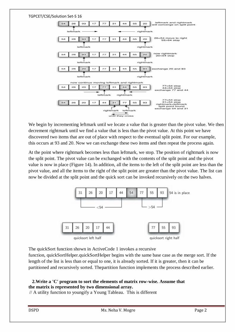
Figure 12 shows that 54 will serve as our first pivot value. Since we have looked at this example a few
times already, we know that 54 will eventually end up in the position currently holding 31.
The partitionprocess will happen next. It will find the split point and at the same time move other
items to the appropriate side of the list, either less than or greater than the pivot value.
Partitioning begins by locating two position markers—let’s call them leftmark and rightmark—at the
beginning and end of the remaining items in the list (positions 1 and 8 in Figure 13). The goal of the
partition process is to move items that are on the wrong side with respect to the pivot value while also
converging on the split point. Figure 13 shows this process as we locate the position of 54.
TGPCET/CSE/Solution Set-S 16
DSPD Ms. Neha V. Mogre Page 2
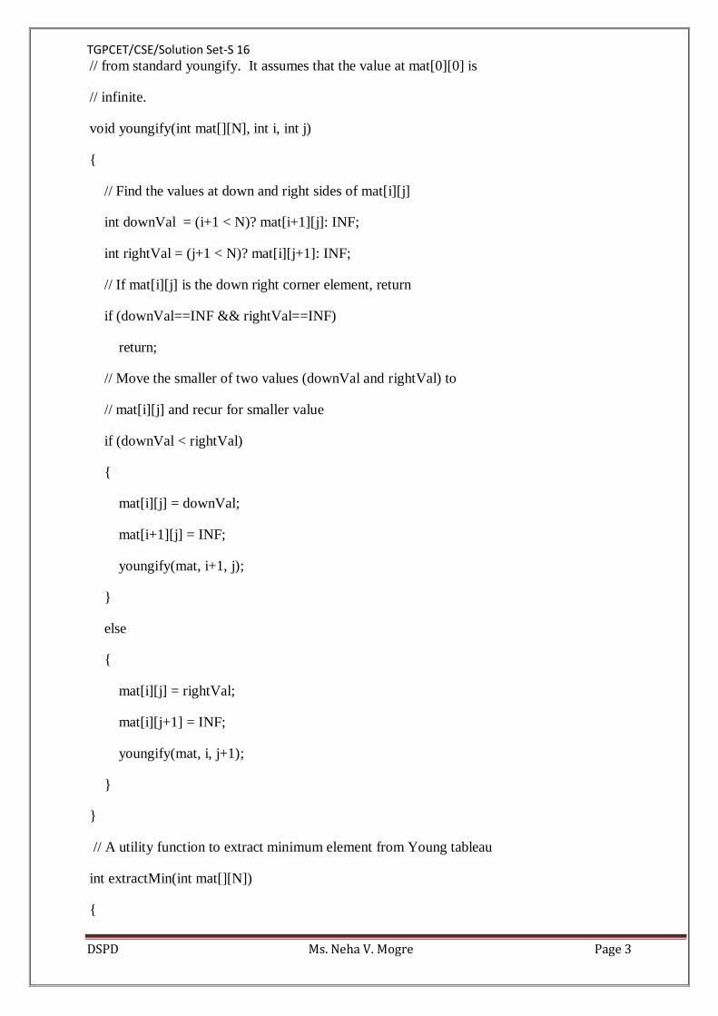
We begin by incrementing leftmark until we locate a value that is greater than the pivot value. We then
decrement rightmark until we find a value that is less than the pivot value. At this point we have
discovered two items that are out of place with respect to the eventual split point. For our example,
this occurs at 93 and 20. Now we can exchange these two items and then repeat the process again.
At the point where rightmark becomes less than leftmark, we stop. The position of rightmark is now
the split point. The pivot value can be exchanged with the contents of the split point and the pivot
value is now in place (Figure 14). In addition, all the items to the left of the split point are less than the
pivot value, and all the items to the right of the split point are greater than the pivot value. The list can
now be divided at the split point and the quick sort can be invoked recursively on the two halves.
The quickSort function shown in ActiveCode 1 invokes a recursive
function, quickSortHelper.quickSortHelper begins with the same base case as the merge sort. If the
length of the list is less than or equal to one, it is already sorted. If it is greater, then it can be
partitioned and recursively sorted. Thepartition function implements the process described earlier.
2.Write a 'C' program to sort the elements of matrix row-wise. Assume that
the matrix is represented by two dimensional array.
// A utility function to youngify a Young Tableau. This is different
TGPCET/CSE/Solution Set-S 16
DSPD Ms. Neha V. Mogre Page 3
// from standard youngify. It assumes that the value at mat[0][0] is
// infinite.
void youngify(int mat[][N], int i, int j)
{
// Find the values at down and right sides of mat[i][j]
int downVal = (i+1 < N)? mat[i+1][j]: INF;
int rightVal = (j+1 < N)? mat[i][j+1]: INF;
// If mat[i][j] is the down right corner element, return
if (downVal==INF && rightVal==INF)
return;
// Move the smaller of two values (downVal and rightVal) to
// mat[i][j] and recur for smaller value
if (downVal < rightVal)
{
mat[i][j] = downVal;
mat[i+1][j] = INF;
youngify(mat, i+1, j);
}
else
{
mat[i][j] = rightVal;
mat[i][j+1] = INF;
youngify(mat, i, j+1);
}
}
// A utility function to extract minimum element from Young tableau
int extractMin(int mat[][N])
{
TGPCET/CSE/Solution Set-S 16
DSPD Ms. Neha V. Mogre Page 4
int ret = mat[0][0];
mat[0][0] = INF;
youngify(mat, 0, 0);
return ret;
}
// This function uses extractMin() to print elements in sorted order
void printSorted(int mat[][N])
{
cout << "Elements of matrix in sorted order \n";
for (int i=0; i<N*N; i++)
cout << extractMin(mat) << " ";
}
// driver program to test above function
int main()
{
int mat[N][N] = { {10, 20, 30, 40},
{15, 25, 35, 45},
{27, 29, 37, 48},
{32, 33, 39, 50},
};
printSorted(mat);
return 0;
}
Run on IDE
Output:
Elements of matrix in sorted order
10 15 20 25 27 29 30 32 33 35 37 39 40 45 48 50

TGPCET/CSE/Solution Set-S 16
DSPD Ms. Neha V. Mogre Page 5
2. Search the following elements using linear search as well as binary search.
Give the step by step representation for successful as well as unsuccessful
search. Algo specify time complexity of both
80 75 45 90 30 40 12 15 93 08
bool jw_search ( int *list, int size, int key, int*& rec )
{
// Linear Search
bool found = false;
int i;
for ( i = 0; i < size; i++ ) {
if ( key == list[i] )
break;
}
if ( i < size ) {
found = true;
rec = &list[i];
}
return found;
}
Complexity
Best case: 1 step
Average case: n/2 steps
Worse case: n steps
Binary search
bool jw_search ( int *list, int size, int key, int*& rec )
{
// Binary search
bool found = false;
int low = 0, high = size - 1;
TGPCET/CSE/Solution Set-S 16
DSPD Ms. Neha V. Mogre Page 6
while ( high >= low ) {
int mid = ( low + high ) / 2;
if ( key < list[mid] )
high = mid - 1;
else if ( key > list[mid] )
low = mid + 1;
else {
found = true;
rec = &list[mid];
break;
}
}
return found;
}
Best case: log2n steps (could be 1 step)
Average case: log2n steps (could be log2n / 2 steps)
Worse case: log2n steps
3A)
Explain with example:
i) Circular linked list
In a standard queue data structure re-buffering problem occurs for each dequeue operation. To solve
this problem by joining the front and rear ends of a queue to make the queue as a circular queue
Circular queue is a linear data structure. It follows FIFO principle.
In circular queue the last node is connected back to the first node to make a circle.
Circular linked list fallow the First In First Out principle
Elements are added at the rear end and the elements are deleted at front end of the queue
Both the front and the rear pointers points to the beginning of the array.
It is also called as “Ring buffer”.
Items can inserted and deleted from a queue in O(1) time.
Circular Queue can be created in three ways they are
Using single linked list
TGPCET/CSE/Solution Set-S 16
DSPD Ms. Neha V. Mogre Page 7
Using double linked list
Using arrays
Using single linked list:
It is an extension for the basic single linked list. In circular linked list Instead of storing a Null value in
the last node of a single linked list, store the address of the 1st node (root) forms a circular linked list.
Using circular linked list it is possible to directly traverse to the first node after reaching the last node.
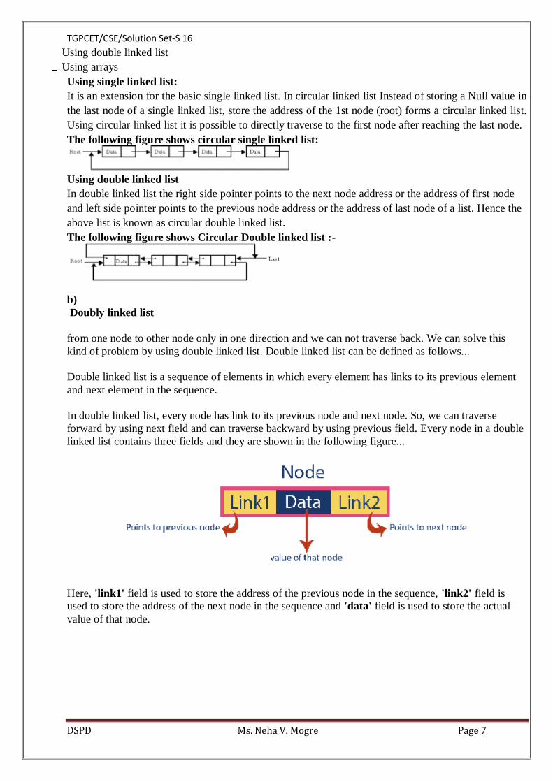
The following figure shows circular single linked list:
Using double linked list
In double linked list the right side pointer points to the next node address or the address of first node
and left side pointer points to the previous node address or the address of last node of a list. Hence the
above list is known as circular double linked list.
The following figure shows Circular Double linked list :-
b)
Doubly linked list
from one node to other node only in one direction and we can not traverse back. We can solve this
kind of problem by using double linked list. Double linked list can be defined as follows...
Double linked list is a sequence of elements in which every element has links to its previous element
and next element in the sequence.
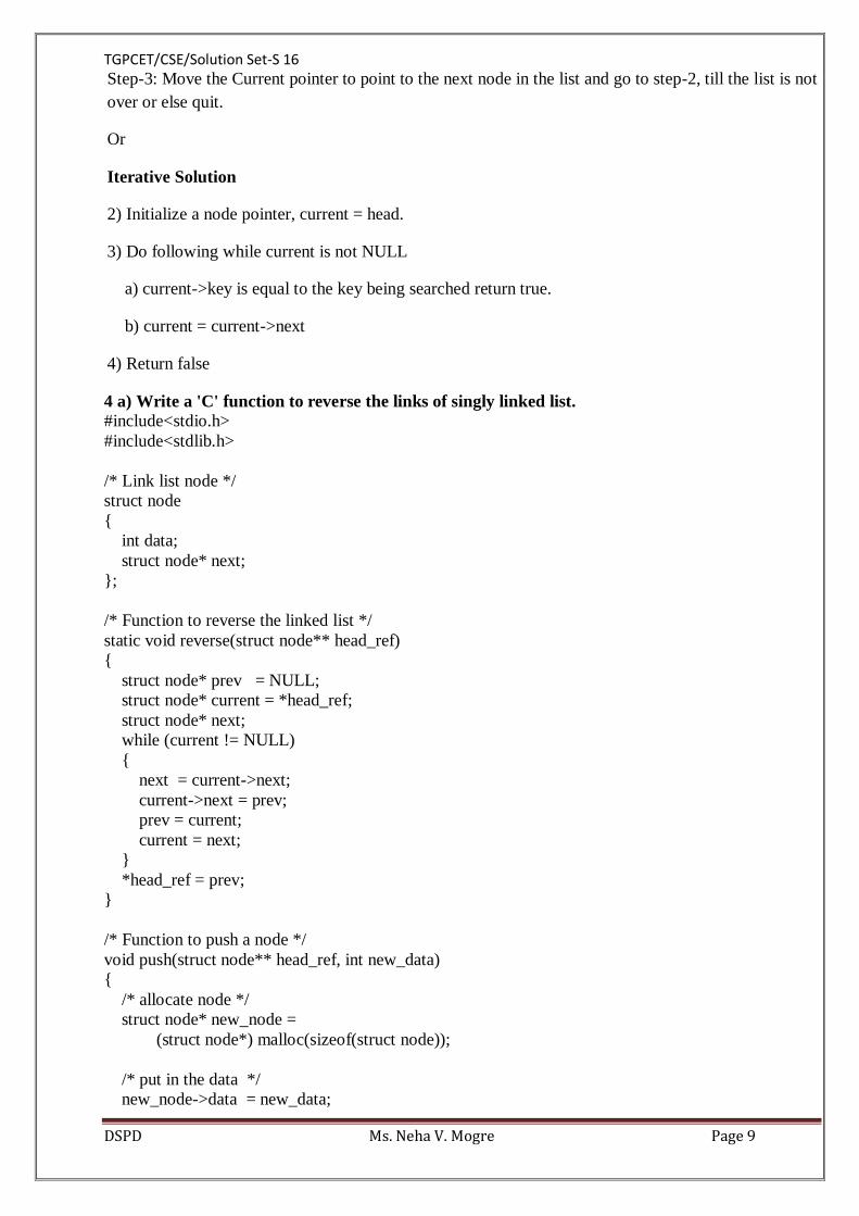
In double linked list, every node has link to its previous node and next node. So, we can traverse
forward by using next field and can traverse backward by using previous field. Every node in a double
linked list contains three fields and they are shown in the following figure...
Here, 'link1' field is used to store the address of the previous node in the sequence, 'link2' field is
used to store the address of the next node in the sequence and 'data' field is used to store the actual
value of that node.

TGPCET/CSE/Solution Set-S 16
DSPD Ms. Neha V. Mogre Page 8
Example
NOTE
☀ In double linked list, the first node must be always pointed by head.
☀ Always the previous field of the first node must be NULL.
☀ Always the next field of the last node must be NULL.
Operations
In a double linked list, we perform the following operations...
1. Insertion
2. Deletion
3. Display
4.
3) Generalized linked list
Current implementation of lists: – Finite sequence of zero or more atomic elements A = (a 0, a 1, a
2 …. an-1 ) – Elements of list are restricted to atoms: • Individual pieces of information – An
integer, A Rectangle • Only structural property of a list is position – Given position, can easily
access data • Very much like arrays Generalized Lists • Relax the assumption of atomic elements: –
Lists can now be composed of atoms or lists – Definition: A generalized list A is a finite sequence
of zero or more elements a 0, a 1, …, an-1 where ai is either an atom or a list. Elements that are not
atomic are called sublists of A. Generalized Lists • Conventions for Generalized Lists: – List names
are represented in capital letters – Atom names are lowercase letters • Definitions for Generalized
Lists: Length – Number of elements (atoms or sublists) in the list If length > 0 Head – First element
of the list Tail – List composed of all elements except first of list Generalized Lists • Examples of
Generalized Lists: – D = ( ) Length 0, Null List – A = (a, (b,c)) Length 2 Head = a Tail = ((b,c)) – B
= (A, A, ()) Length 3 Head = A Tail = (A,()) – C = (a, C) Length 2 Head = a Tail = (C)
b) Write an algorithm to search an element in singly linked list.
Step-1: Initialise the Current pointer with the beginning of the List.
Step-2: Compare the KEY value with the Current node value;
if they match then quit there
else go to step-3.
TGPCET/CSE/Solution Set-S 16
DSPD Ms. Neha V. Mogre Page 9
Step-3: Move the Current pointer to point to the next node in the list and go to step-2, till the list is not
over or else quit.
Or
Iterative Solution
2) Initialize a node pointer, current = head.
3) Do following while current is not NULL
a) current->key is equal to the key being searched return true.
b) current = current->next
4) Return false
4 a) Write a 'C' function to reverse the links of singly linked list.
#include<stdio.h>
#include<stdlib.h>
/* Link list node */
struct node
{
int data;
struct node* next;
};
/* Function to reverse the linked list */
static void reverse(struct node** head_ref)
{
struct node* prev = NULL;
struct node* current = *head_ref;
struct node* next;
while (current != NULL)
{
next = current->next;
current->next = prev;
prev = current;
current = next;
}
*head_ref = prev;
}
/* Function to push a node */
void push(struct node** head_ref, int new_data)
{
/* allocate node */
struct node* new_node =
(struct node*) malloc(sizeof(struct node));
/* put in the data */
new_node->data = new_data;
TGPCET/CSE/Solution Set-S 16
DSPD Ms. Neha V. Mogre Page 10
/* link the old list off the new node */
new_node->next = (*head_ref);
/* move the head to point to the new node */
(*head_ref) = new_node;
}
/* Function to print linked list */
void printList(struct node *head)
{
struct node *temp = head;
while(temp != NULL)
{
printf("%d ", temp->data);
temp = temp->next;
}
}
/* Driver program to test above function*/
int main()
{
/* Start with the empty list */
struct node* head = NULL;
push(&head, 20);
push(&head, 4);
push(&head, 15);
push(&head, 85);
printf("Given linked list\n");
printList(head);
reverse(&head);
printf("\nReversed Linked list \n");
printList(head);
getchar();
}
Run on IDE
Given linked list
85 15 4 20
Reversed Linked list
20 4 15 85
Time Complexity: O(n) Space Complexity: O(1)
b) Write an algorithm for insertion in the doubly linked list.
i) Insertion at beginning.
ii) Insertion at eng
iii) Insertion at specific location.
TGPCET/CSE/Solution Set-S 16
DSPD Ms. Neha V. Mogre Page 11
Inserting At Beginning of the list
We can use the following steps to insert a new node at beginning of the double linked list...
Step 1: Create a newNode with given value and newNode → previous as NULL.
Step 2: Check whether list is Empty (head == NULL)
Step 3: If it is Empty then, assign NULL to newNode → next and newNode to head.
Step 4: If it is not Empty then, assign head to newNode → next and newNode to head.
Inserting At End of the list
We can use the following steps to insert a new node at end of the double linked list...
Step 1: Create a newNode with given value and newNode → next as NULL.
Step 2: Check whether list is Empty (head == NULL)
Step 3: If it is Empty, then assign NULL to newNode → previous and newNode to head.
Step 4: If it is not Empty, then, define a node pointer temp and initialize with head.
Step 5: Keep moving the temp to its next node until it reaches to the last node in the list (until
temp → next is equal to NULL).
Step 6: Assign newNode to temp → next and temp to newNode → previous.
Inserting At Specific location in the list (After a Node)
We can use the following steps to insert a new node after a node in the double linked list...
Step 1: Create a newNode with given value.
Step 2: Check whether list is Empty (head == NULL)
Step 3: If it is Empty then, assign NULL to newNode → previous & newNode → next and
newNode to head.
Step 4: If it is not Empty then, define two node pointers temp1 & temp2 and initialize temp1
with head.
Step 5: Keep moving the temp1 to its next node until it reaches to the node after which we
want to insert the newNode (until temp1 → data is equal to location, here location is the node
value after which we want to insert the newNode).
Step 6: Every time check whether temp1 is reached to the last node. If it is reached to the last
node then display 'Given node is not found in the list!!! Insertion not possible!!!' and
terminate the function. Otherwise move the temp1 to next node.
Step 7: Assign temp1 → next to temp2, newNode to temp1 → next, temp1 to newNode →
previous, temp2 to newNode → next and newNode to temp2 → previous.
5) In a circular queue represented by an array, how can one specify the number of elements in
the queue in terms of front, rear and MaxQ? Write a 'C' function to delete the element from the
circular queue.
A Circular Queue can be defined as follows...
TGPCET/CSE/Solution Set-S 16
DSPD Ms. Neha V. Mogre Page 12
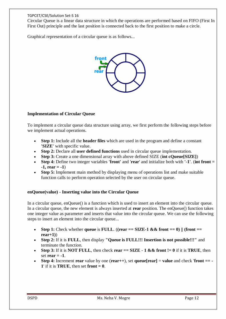
Circular Queue is a linear data structure in which the operations are performed based on FIFO (First In
First Out) principle and the last position is connected back to the first position to make a circle.
Graphical representation of a circular queue is as follows...
Implementation of Circular Queue
To implement a circular queue data structure using array, we first perform the following steps before
we implement actual operations.
Step 1: Include all the header files which are used in the program and define a constant
'SIZE' with specific value.
Step 2: Declare all user defined functions used in circular queue implementation.
Step 3: Create a one dimensional array with above defined SIZE (int cQueue[SIZE])
Step 4: Define two integer variables 'front' and 'rear' and initialize both with '-1'. (int front =
-1, rear = -1)
Step 5: Implement main method by displaying menu of operations list and make suitable
function calls to perform operation selected by the user on circular queue.
enQueue(value) - Inserting value into the Circular Queue
In a circular queue, enQueue() is a function which is used to insert an element into the circular queue.
In a circular queue, the new element is always inserted at rear position. The enQueue() function takes
one integer value as parameter and inserts that value into the circular queue. We can use the following
steps to insert an element into the circular queue...
Step 1: Check whether queue is FULL. ((rear == SIZE-1 && front == 0) || (front ==
rear+1))
Step 2: If it is FULL, then display "Queue is FULL!!! Insertion is not possible!!!" and
terminate the function.
Step 3: If it is NOT FULL, then check rear == SIZE - 1 && front != 0 if it is TRUE, then
set rear = -1.
Step 4: Increment rear value by one (rear++), set queue[rear] = value and check 'front == -
1' if it is TRUE, then set front = 0.

TGPCET/CSE/Solution Set-S 16
DSPD Ms. Neha V. Mogre Page 13
deQueue() - Deleting a value from the Circular Queue
In a circular queue, deQueue() is a function used to delete an element from the circular queue. In a
circular queue, the element is always deleted from front position. The deQueue() function doesn't take
any value as parameter. We can use the following steps to delete an element from the circular queue...
Step 1: Check whether queue is EMPTY. (front == -1 && rear == -1)
Step 2: If it is EMPTY, then display "Queue is EMPTY!!! Deletion is not possible!!!" and
terminate the function.
Step 3: If it is NOT EMPTY, then display queue[front] as deleted element and increment the
front value by one (front ++). Then check whether front == SIZE, if it is TRUE, then set
front = 0. Then check whether both front - 1 and rear are equal (front -1 == rear), if it
TRUE, then set both front and rear to '-1' (front = rear = -1).
display() - Displays the elements of a Circular Queue
We can use the following steps to display the elements of a circular queue...
Step 1: Check whether queue is EMPTY. (front == -1)
Step 2: If it is EMPTY, then display "Queue is EMPTY!!!" and terminate the function.
Step 3: If it is NOT EMPTY, then define an integer variable 'i' and set 'i = front'.
Step 4: Check whether 'front <= rear', if it is TRUE, then display 'queue[i]' value and
increment 'i' value by one (i++). Repeat the same until 'i <= rear' becomes FALSE.
Step 5: If 'front <= rear' is FALSE, then display 'queue[i]' value and increment 'i' value by
one (i++). Repeat the same until'i <= SIZE - 1' becomes FALSE.
Step 6: Set i to 0.
Step 7: Again display 'cQueue[i]' value and increment i value by one (i++). Repeat the same
until 'i <= rear' becomes FALSE.
6. a) Explain :
i) Priority queue
ii) Double ended queue
Double Ended Queue (Dequeue):- Double Ended Queue is also a Queue data structure in which the
insertion and deletion operations are performed at both the ends (front and rear). That means, we can
insert at both front and rear positions and can delete from both front and rear positions.
Double Ended Queue can be represented in TWO ways, those are as follows...
1. Input Restricted Double Ended Queue
2. Output Restricted Double Ended Queue
TGPCET/CSE/Solution Set-S 16
DSPD Ms. Neha V. Mogre Page 14
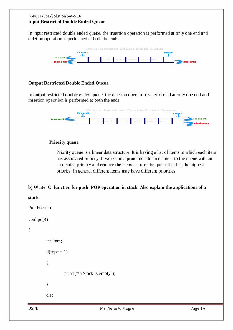
Input Restricted Double Ended Queue
In input restricted double ended queue, the insertion operation is performed at only one end and
deletion operation is performed at both the ends.
Output Restricted Double Ended Queue
In output restricted double ended queue, the deletion operation is performed at only one end and
insertion operation is performed at both the ends.
Priority queue
Priority queue is a linear data structure. It is having a list of items in which each item
has associated priority. It works on a principle add an element to the queue with an
associated priority and remove the element from the queue that has the highest
priority. In general different items may have different priorities.
b) Write 'C' function for push' POP operation in stack. Also explain the applications of a
stack.
Pop Fuction
void pop()
{
int item;
if(top==-1)
{
printf("\n Stack is empty");
}
else
TGPCET/CSE/Solution Set-S 16
DSPD Ms. Neha V. Mogre Page 15
{
item=stack[top];
printf("\n item popped is=%d", item);
top--;
}
}
Implementation of stack using'c'
/* static implementation of stack*/
#include<stdio.h>
#include<conio.h>
#define size 5
int stack[size];
int top;
void push()
{
int n;
printf("\n Enter item in stack");
scanf("%d",&n);
if(top==size-1)
{
printf("\nStack is Full");
}
else

TGPCET/CSE/Solution Set-S 16
DSPD Ms. Neha V. Mogre Page 16
{
top=top+1;
stack[top]=n;
}
}
void pop()
{
int item;
if(top==-1)
{
printf("\n Stack is empty");
}
else
{
item=stack[top];
printf("\n item popped is=%d", item);
top--;
}
}
void display()
{
int i;
printf("\n item in stack are");
for(i=top; i>=0; i--)
printf("\n %d", stack[i]);
}
TGPCET/CSE/Solution Set-S 16
DSPD Ms. Neha V. Mogre Page 17
void main()
{
char ch,ch1;
ch ='y';
ch1='y';
top=-1;
clrscr();
while(ch!='n')
{
push();
printf("\n Do you want to push any item in stack y/n");
ch=getch();
}
display();
while(ch1!='n')
{
printf("\n Do you want to delete any item in stack y/n");
ch1=getch();
pop();
}
display();
getch();
}
7b) Write a 'C' function to determine the depth of the binary tree as well as to count the
number of leaf nodes in the tree.

TGPCET/CSE/Solution Set-S 16
DSPD Ms. Neha V. Mogre Page 18
/*
* C Program to Find the Number of Nodes in a Binary Tree
*/
#include <stdio.h>
#include <stdlib.h>
/*
* Structure of node
*/
struct btnode
{
int value;
struct btnode *l;
struct btnode *r;
};
void createbinary();
void preorder(node *);
int count(node*);
node* add(int);
typedef struct btnode node;
node *ptr, *root = NULL;
int main()
{
int c;
createbinary();
preorder(root);
c = count(root);
printf("\nNumber of nodes in binary tree are:%d\n", c);

TGPCET/CSE/Solution Set-S 16
DSPD Ms. Neha V. Mogre Page 19
}
/*
* constructing the following binary tree
* 50
* / \
* 20 30
* / \
* 70 80
* / \ \
*10 40 60
*/
void createbinary()
{
root = add(50);
root->l = add(20);
root->r = add(30);
root->l->l = add(70);
root->l->r = add(80);
root->l->l->l = add(10);
root->l->l->r = add(40);
root->l->r->r = add(60);
}
/*
* Add the node to binary tree
*/
node* add(int val)
{

TGPCET/CSE/Solution Set-S 16
DSPD Ms. Neha V. Mogre Page 20
ptr = (node*)malloc(sizeof(node));
if (ptr == NULL)
{
printf("Memory was not allocated");
return;
}
ptr->value = val;
ptr->l = NULL;
ptr->r = NULL;
return ptr;
}
/*
* counting the number of nodes in a tree
*/
int count(node *n)
{
int c = 1;
if (n == NULL)
return 0;
else
{
c += count(n->l);
c += count(n->r);
return c;
}
}
TGPCET/CSE/Solution Set-S 16
DSPD Ms. Neha V. Mogre Page 21
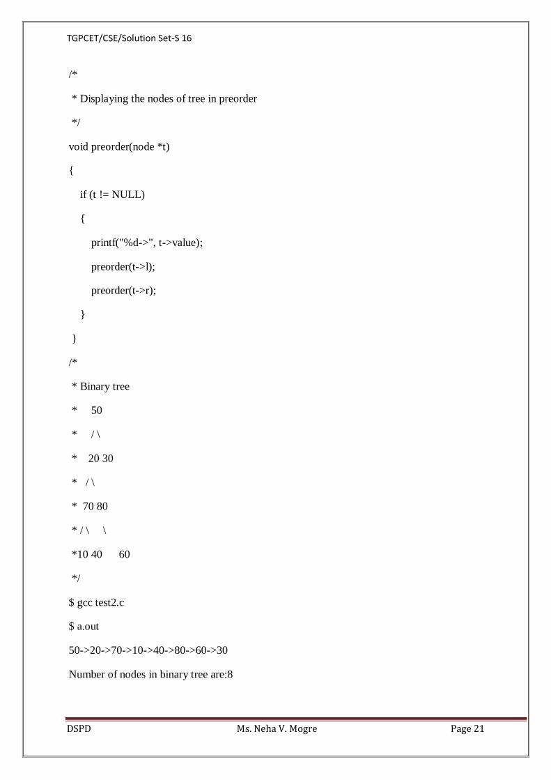
/*
* Displaying the nodes of tree in preorder
*/
void preorder(node *t)
{
if (t != NULL)
{
printf("%d->", t->value);
preorder(t->l);
preorder(t->r);
}
}
/*
* Binary tree
* 50
* / \
* 20 30
* / \
* 70 80
* / \ \
*10 40 60
*/
$ gcc test2.c
$ a.out
50->20->70->10->40->80->60->30
Number of nodes in binary tree are:8

TGPCET/CSE/Solution Set-S 16
DSPD Ms. Neha V. Mogre Page 22
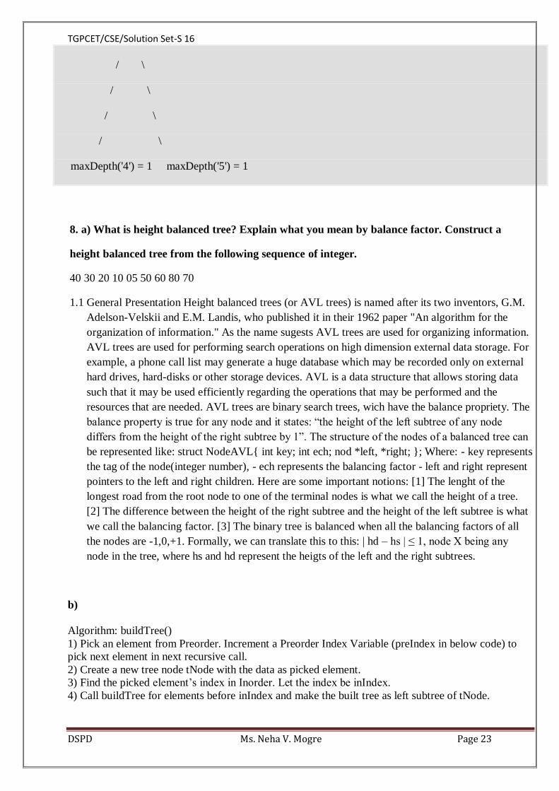
maxDepth()
1. If tree is empty then return 0
2. Else
(a) Get the max depth of left subtree recursively i.e.,
call maxDepth( tree->left-subtree)
(a) Get the max depth of right subtree recursively i.e.,
call maxDepth( tree->right-subtree)
(c) Get the max of max depths of left and right
subtrees and add 1 to it for the current node.
max_depth = max(max dept of left subtree,
max depth of right subtree)
+ 1
(d) Return max_depth
See the below diagram for more clarity about execution of the recursive function maxDepth() for
above example tree.
maxDepth('1') = max(maxDepth('2'), maxDepth('3')) + 1
= 2 + 1
/ \
/ \
/ \
/ \
/ \
maxDepth('1') maxDepth('3') = 1
= max(maxDepth('4'), maxDepth('5')) + 1
= 1 + 1 = 2
/ \
TGPCET/CSE/Solution Set-S 16
DSPD Ms. Neha V. Mogre Page 23
/ \
/ \
/ \
/ \
maxDepth('4') = 1 maxDepth('5') = 1
8. a) What is height balanced tree? Explain what you mean by balance factor. Construct a
height balanced tree from the following sequence of integer.
40 30 20 10 05 50 60 80 70
1.1 General Presentation Height balanced trees (or AVL trees) is named after its two inventors, G.M.
Adelson-Velskii and E.M. Landis, who published it in their 1962 paper "An algorithm for the
organization of information." As the name sugests AVL trees are used for organizing information.
AVL trees are used for performing search operations on high dimension external data storage. For
example, a phone call list may generate a huge database which may be recorded only on external
hard drives, hard-disks or other storage devices. AVL is a data structure that allows storing data
such that it may be used efficiently regarding the operations that may be performed and the
resources that are needed. AVL trees are binary search trees, wich have the balance propriety. The
balance property is true for any node and it states: “the height of the left subtree of any node
differs from the height of the right subtree by 1”. The structure of the nodes of a balanced tree can
be represented like: struct NodeAVL{ int key; int ech; nod *left, *right; }; Where: - key represents
the tag of the node(integer number), - ech represents the balancing factor - left and right represent
pointers to the left and right children. Here are some important notions: [1] The lenght of the
longest road from the root node to one of the terminal nodes is what we call the height of a tree.
[2] The difference between the height of the right subtree and the height of the left subtree is what
we call the balancing factor. [3] The binary tree is balanced when all the balancing factors of all
the nodes are -1,0,+1. Formally, we can translate this to this: | hd – hs | ≤ 1, node X being any
node in the tree, where hs and hd represent the heigts of the left and the right subtrees.
b)
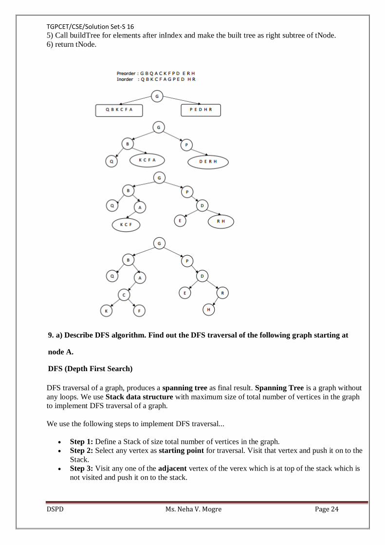
Algorithm: buildTree()
1) Pick an element from Preorder. Increment a Preorder Index Variable (preIndex in below code) to
pick next element in next recursive call.
2) Create a new tree node tNode with the data as picked element.
3) Find the picked element’s index in Inorder. Let the index be inIndex.
4) Call buildTree for elements before inIndex and make the built tree as left subtree of tNode.
TGPCET/CSE/Solution Set-S 16
DSPD Ms. Neha V. Mogre Page 24
5) Call buildTree for elements after inIndex and make the built tree as right subtree of tNode.
6) return tNode.
9. a) Describe DFS algorithm. Find out the DFS traversal of the following graph starting at
node A.
DFS (Depth First Search)
DFS traversal of a graph, produces a spanning tree as final result. Spanning Tree is a graph without
any loops. We use Stack data structure with maximum size of total number of vertices in the graph
to implement DFS traversal of a graph.
We use the following steps to implement DFS traversal...
Step 1: Define a Stack of size total number of vertices in the graph.
Step 2: Select any vertex as starting point for traversal. Visit that vertex and push it on to the
Stack.
Step 3: Visit any one of the adjacent vertex of the verex which is at top of the stack which is
not visited and push it on to the stack.

TGPCET/CSE/Solution Set-S 16
DSPD Ms. Neha V. Mogre Page 25
Step 4: Repeat step 3 until there are no new vertex to be visit from the vertex on top of the
stack.
Step 5: When there is no new vertex to be visit then use back tracking and pop one vertex
from the stack.
Step 6: Repeat steps 3, 4 and 5 until stack becomes Empty.
Step 7: When stack becomes Empty, then produce final spanning tree by removing unused edges from
the graph
b) Write an Bellman ford Algorithm to find single source shortest path in a graph.
Introduction
This post about Bellman Ford Algorithm is a continuation of the post Shortest Path Using Dijkstra’s
Algorithm. While learning about the Dijkstra’s way, we learnt that it is really efficient an algorithm to
find the single source shortest path in any graph provided it has no negative weight edges and no
negative weight cycles.
The running time of the Dijkstra’s Algorithm is also promising, O(E +VlogV) depending on our
choice of data structure to implement the required Priority Queue.
Why Bellman Ford Algorithm?
There can be scenarios where a graph may contain negative weight cycles, of course we do not see this
in a real life simpler graph problems where we need to find the shortest or the cheapest paths between
cities etc. But yes, there are complex real life applications where we will have scenarios like negative
edges and negative edge cycles. Few of them are Linear Programming or Solving the Difference
Constraints (for VLSI designs etc) or Detecting Network Failures.
Understanding the meaning of negative edge weights in a graph
I am sure at first it is very difficult to understand the significance of a negative edge weight. But
consider the below scenario:
A student trying to manage his expenses, where he has to work part time to pay for his fee. His
situation and the maintenance of account can be represented by a graph where the money he earns
during a period can be represented by a positive edge weight and the money he spends can be a
negative edge weight.
There can be many similar situations where we can see negative edge weights and sometimes negative
weight cycles.

TGPCET/CSE/Solution Set-S 16
DSPD Ms. Neha V. Mogre Page 26
What is Negative Weight Cycle
A negative weight cycle means that if we add the weights of all the edges in the cycle the sum will
turn up to be a negative number. See the below graph, it contains a negative weight cycle (C, G, H, C)
with weight -4.
So, how is Bellman Ford solving the negative weight cycles problem?
Actually its not, the algorithm cannot solve this problem and cannot give you a definite path. It is
theoretically impossible to find out the shortest path if there exists a negative weight cycle. If you
happen to find the shortest path, then you can go through the negative cycle once more and get a
smaller path. You can keep repeating this step and go through the cycle every time and reduce the total
weight of the path to negative infinity.
So, in practical scenarios, this algorithm will either give you a valid shortest path or will indicate
that there is a negative weight cycle. Explanation – Shortest Path Using Bellman Ford Algorithm
We can use Bellman Ford for directed as well as un-directed graphs. Let us solve a problem using
directed graphs here. The idea of the algorithm is fairly simple.
1. It maintains a list of unvisited vertices.
2. It chooses a vertex (the source) and assigns a maximum possible cost (i.e. infinity) to every
other vertex.
3. The cost of the source remains zero as it actually takes nothing to reach from the source vertex
to itself.
TGPCET/CSE/Solution Set-S 16
DSPD Ms. Neha V. Mogre Page 27
4. In every subsequent iteration of the algorithm it tries to relax each edge in the graph (by
minimizing the cost of the vertex on which the edge is incident).
5. It repeats step 4 for |V|-1 times. By the last iteration we would have gotten some shortest path
from Source to each vertex.
The formula for relaxation remains same as Dijkstra’s Algorithm.
So, why does the outer loop runs |V| – 1 times?
The argument would be, that the shortest path in the graph with |V| vertices cannot be more lengthy
than |V| – 1. So, if we relax all the edges |V| – 1 times, we would have covered all possibilities of
relaxing the edges and we would be left with all shortest paths. There are many proofs by Induction
available in case you are more interested. Or you can look forward for my next post about “The
correctness of Bellman Ford Algorithm”.
10. a) Explain with example.
i) Hamiltonian cycle
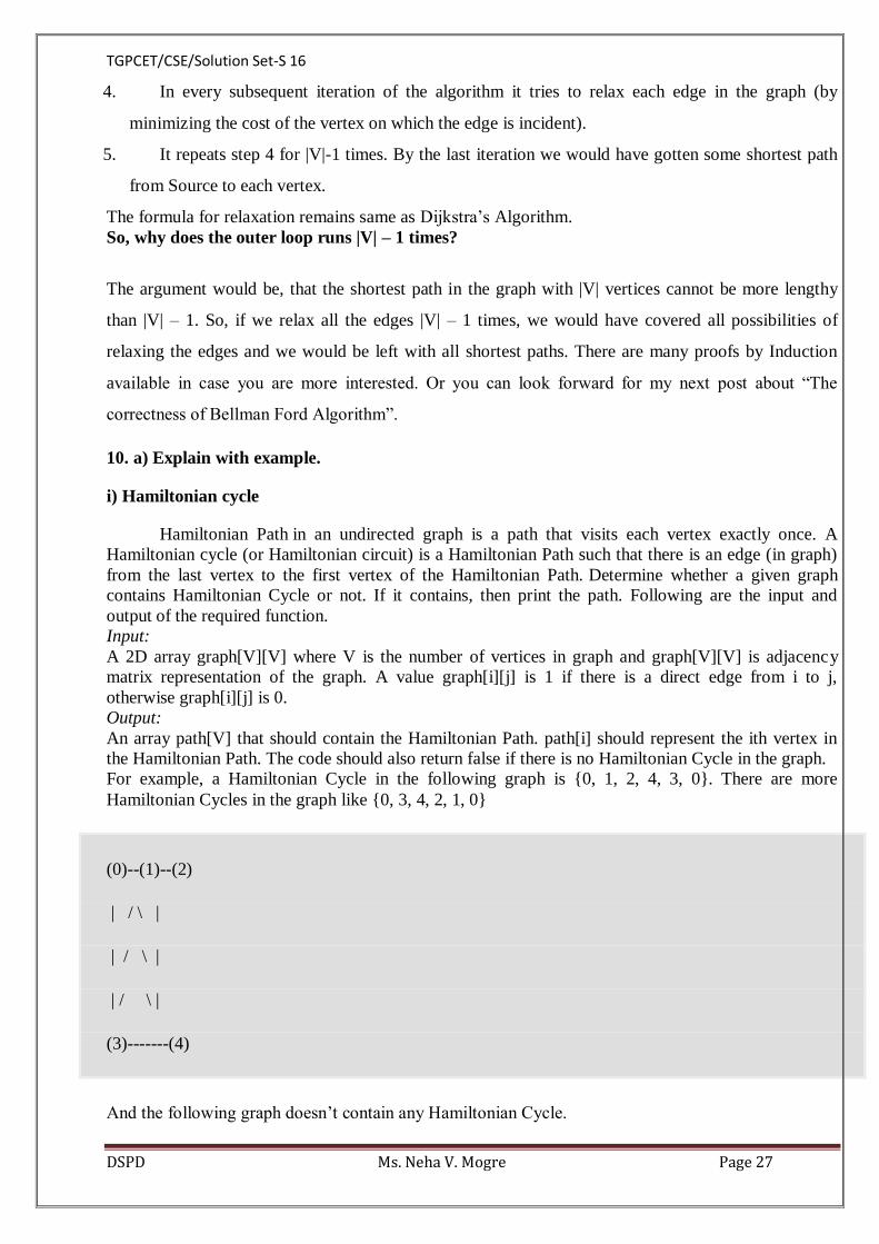
Hamiltonian Path in an undirected graph is a path that visits each vertex exactly once. A
Hamiltonian cycle (or Hamiltonian circuit) is a Hamiltonian Path such that there is an edge (in graph)
from the last vertex to the first vertex of the Hamiltonian Path. Determine whether a given graph
contains Hamiltonian Cycle or not. If it contains, then print the path. Following are the input and
output of the required function.
Input:
A 2D array graph[V][V] where V is the number of vertices in graph and graph[V][V] is adjacency
matrix representation of the graph. A value graph[i][j] is 1 if there is a direct edge from i to j,
otherwise graph[i][j] is 0.
Output:
An array path[V] that should contain the Hamiltonian Path. path[i] should represent the ith vertex in
the Hamiltonian Path. The code should also return false if there is no Hamiltonian Cycle in the graph.
For example, a Hamiltonian Cycle in the following graph is {0, 1, 2, 4, 3, 0}. There are more
Hamiltonian Cycles in the graph like {0, 3, 4, 2, 1, 0}
(0)--(1)--(2)
| / \ |
| / \ |
| / \ |
(3)-------(4)
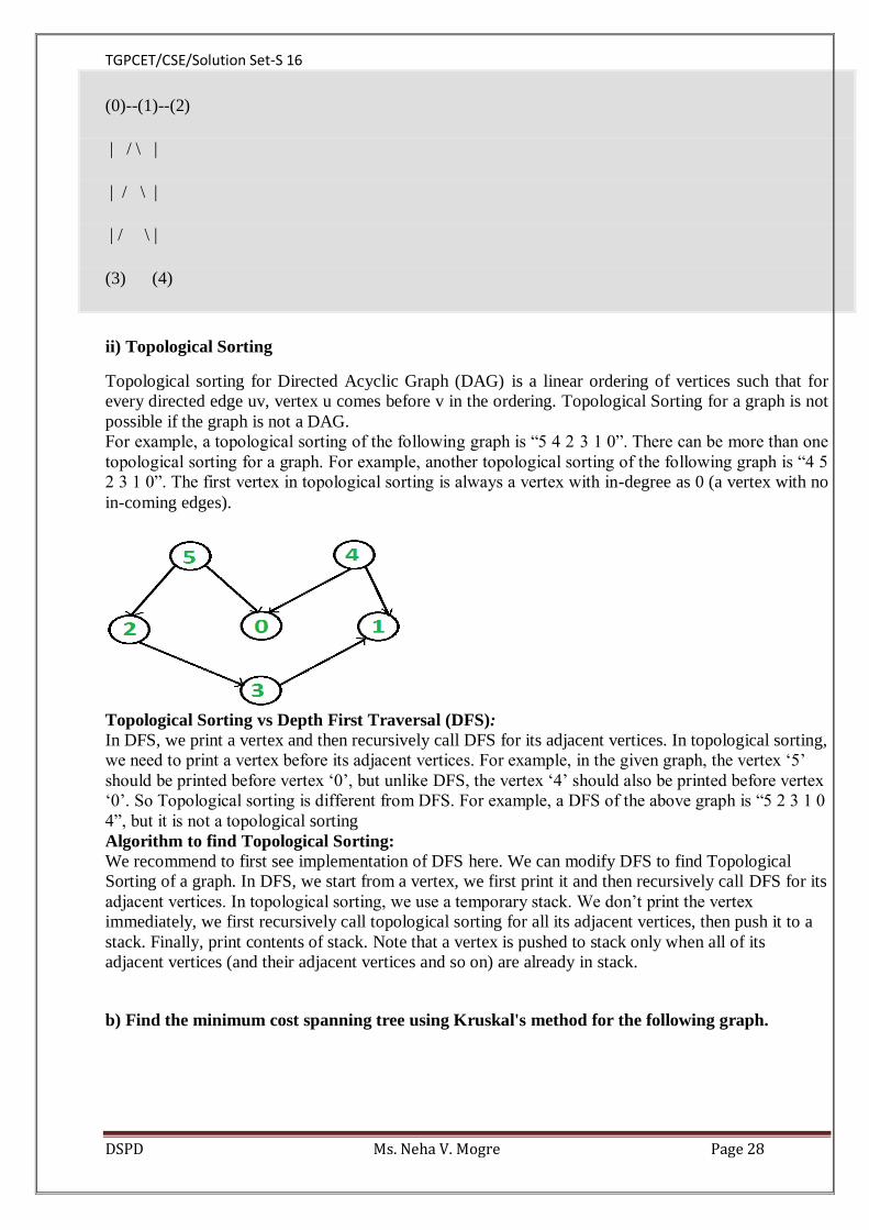
And the following graph doesn’t contain any Hamiltonian Cycle.
TGPCET/CSE/Solution Set-S 16
DSPD Ms. Neha V. Mogre Page 28
(0)--(1)--(2)
| / \ |
| / \ |
| / \ |
(3) (4)
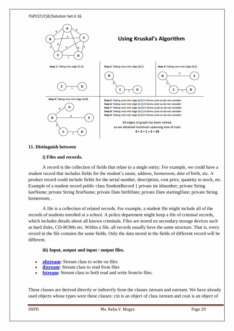
ii) Topological Sorting
Topological sorting for Directed Acyclic Graph (DAG) is a linear ordering of vertices such that for
every directed edge uv, vertex u comes before v in the ordering. Topological Sorting for a graph is not
possible if the graph is not a DAG.
For example, a topological sorting of the following graph is “5 4 2 3 1 0”. There can be more than one
topological sorting for a graph. For example, another topological sorting of the following graph is “4 5
2 3 1 0”. The first vertex in topological sorting is always a vertex with in-degree as 0 (a vertex with no
in-coming edges).
Topological Sorting vs Depth First Traversal (DFS):
In DFS, we print a vertex and then recursively call DFS for its adjacent vertices. In topological sorting,
we need to print a vertex before its adjacent vertices. For example, in the given graph, the vertex ‘5’
should be printed before vertex ‘0’, but unlike DFS, the vertex ‘4’ should also be printed before vertex
‘0’. So Topological sorting is different from DFS. For example, a DFS of the above graph is “5 2 3 1 0
4”, but it is not a topological sorting
Algorithm to find Topological Sorting:
We recommend to first see implementation of DFS here. We can modify DFS to find Topological
Sorting of a graph. In DFS, we start from a vertex, we first print it and then recursively call DFS for its
adjacent vertices. In topological sorting, we use a temporary stack. We don’t print the vertex
immediately, we first recursively call topological sorting for all its adjacent vertices, then push it to a
stack. Finally, print contents of stack. Note that a vertex is pushed to stack only when all of its
adjacent vertices (and their adjacent vertices and so on) are already in stack.
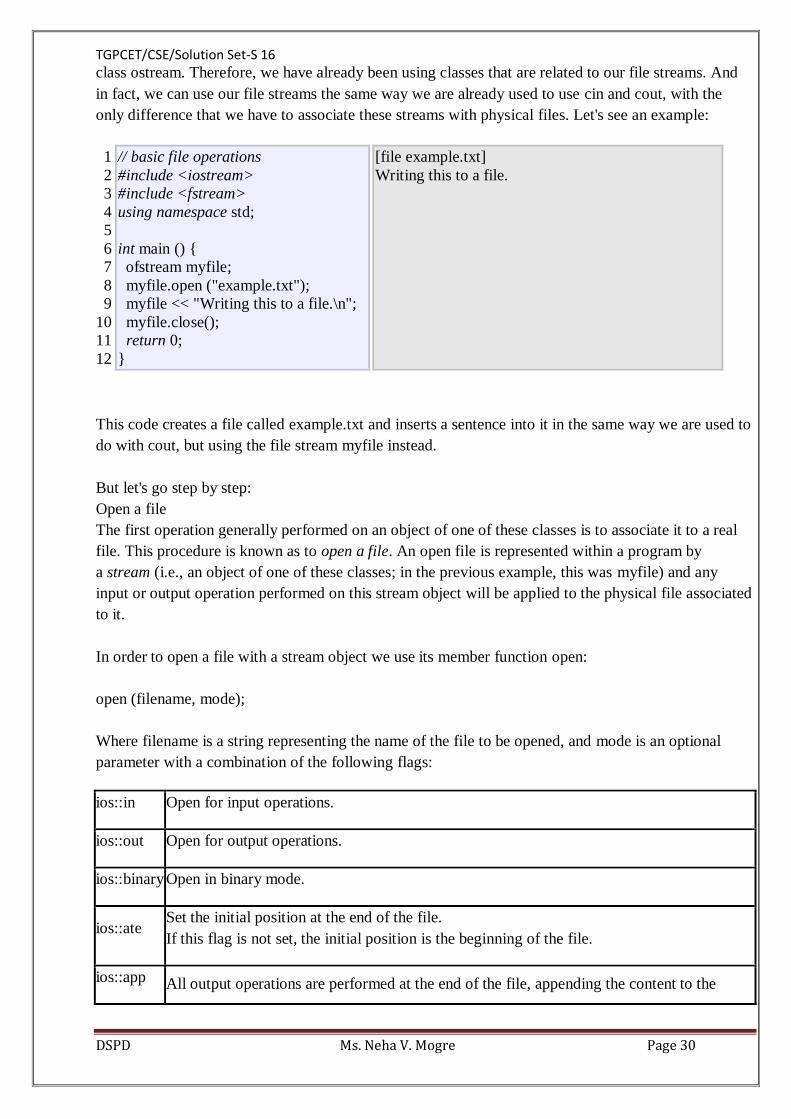
b) Find the minimum cost spanning tree using Kruskal's method for the following graph.
TGPCET/CSE/Solution Set-S 16
DSPD Ms. Neha V. Mogre Page 29
11. Distinguish between
i) Files and records.
A record is the collection of fields that relate to a single entity. For example, we could have a
student record that includes fields for the student’s name, address, homeroom, date of birth, etc. A
product record could include fields for the serial number, description, cost price, quantity in stock, etc.
Example of a student record public class StudentRecord { private int idnumber; private String
lastName; private String firstName; private Date birthDate; private Date startingDate; private String
homeroom; .
A file is a collection of related records. For example, a student file might include all of the
records of students enrolled at a school. A police department might keep a file of criminal records,
which includes details about all known criminals. Files are stored on secondary storage devices such
as hard disks, CD-ROMs etc. Within a file, all records usually have the same structure. That is, every
record in the file contains the same fields. Only the data stored in the fields of different record will be
different.
iii) Input, output and input / output files.
ofstream: Stream class to write on files
ifstream: Stream class to read from files
fstream: Stream class to both read and write from/to files.
These classes are derived directly or indirectly from the classes istream and ostream. We have already
used objects whose types were these classes: cin is an object of class istream and cout is an object of
TGPCET/CSE/Solution Set-S 16
DSPD Ms. Neha V. Mogre Page 30
class ostream. Therefore, we have already been using classes that are related to our file streams. And
in fact, we can use our file streams the same way we are already used to use cin and cout, with the
only difference that we have to associate these streams with physical files. Let's see an example:
1
2
3
4
5
6
7
8
9
10
11
12
// basic file operations
#include <iostream>
#include <fstream>
using namespace std;
int main () {
ofstream myfile;
myfile.open ("example.txt");
myfile << "Writing this to a file.\n";
myfile.close();
return 0;
}
[file example.txt]
Writing this to a file.
This code creates a file called example.txt and inserts a sentence into it in the same way we are used to
do with cout, but using the file stream myfile instead.
But let's go step by step:
Open a file
The first operation generally performed on an object of one of these classes is to associate it to a real
file. This procedure is known as to open a file. An open file is represented within a program by
a stream (i.e., an object of one of these classes; in the previous example, this was myfile) and any
input or output operation performed on this stream object will be applied to the physical file associated
to it.
In order to open a file with a stream object we use its member function open:
open (filename, mode);
Where filename is a string representing the name of the file to be opened, and mode is an optional
parameter with a combination of the following flags:
ios::in Open for input operations.
ios::out Open for output operations.
ios::binary Open in binary mode.
ios::ate Set the initial position at the end of the file.
If this flag is not set, the initial position is the beginning of the file.
ios::app All output operations are performed at the end of the file, appending the content to the

TGPCET/CSE/Solution Set-S 16
DSPD Ms. Neha V. Mogre Page 31
current content of the file.
ios::trunc If the file is opened for output operations and it already existed, its previous content is
deleted and replaced by the new one.
ii) Sequential and Random access.
a sequential file is one where you start at the beginning and read each record IN SEQUENCE.
The same idea as playing a song on a Tape, or a movie on a VCR - in order to read record 12, you
MUST read records 1 through 11, in that precise order, first.
A random access file allows you to read ANY record, in ANY order, with having to have read any
other records first.
Think of it like houses along a street. You can go up to any house, without having to have gone up to
any other house, first.
With a Random Access file, you MUST know how long a record is, and the ALL MUST be tha same
length, so that you can easily go to the 12th record, without having to read the first 11.
In a Sequential fiel, each record can be of different length, because the length of arecord is not
important. In order to read the 12th record, you MUST read the first 11 records, no matter how long
each to those 11 records is.
the lof function returns the Length Of The file (LOF=LengthOfFile), in bytes.
12. a) Why B+ tree is considered a better structure than B-tree for implementation of an
indexed sequential.
B-tree is a tree data structure that keeps data sorted and allows searches, sequential access,
insertions, and deletions in logarithmic amortized time. The B-tree is a generalization of a binary
search tree in that a node can have more than two children.
B+ tree or B plus tree is a type of tree which represents sorted data in a way that allows for
efficient insertion, retrieval and removal of records, each of which is identified by a key. It is a
dynamic, multilevel index, with maximum and minimum bounds on the number of keys in each index
segment (usually called a "block" or "node").
In a B+ tree, in contrast to a B-tree, all records are stored at the leaf level of the tree; only keys
are stored in interior nodes.
Advantages of B+-trees:1) Any record can be fetched in equal number of disk accesses.2)
Range queries can be performed easily as leaves are linked up3) Height of the tree is less as only keys
are used for indexing4) Supports both random and sequential access

TGPCET/CSE/Solution Set-S 16
DSPD Ms. Neha V. Mogre Page 32
.Disadvantages of B+-trees:Insert and delete operations are complicatedRoot node becomes a
hotspot
OR
Key difference: In computers, the binary trees are tree data structures that store the data, and
allow the user to access, search, insert and delete the data at the algorithmic time. The difference
between a B and B+ tree is that, in a B-tree, both the keys and data in the internal/leaf nodes can be
stored, whereas in a B+ tree only the leaf nodes can be stored.
The Binary trees are balanced search trees, which are designed to work well on direct access
secondary storage devices such as the magnetic disks. Rudolf Bayer and Ed McCreight invented the
concept of a B-tree.
B Tree
b) Explain collision resolution and hash function.
HASH TABLE:
It is a Data structure where the data elements are stored(inserted), searched, deleted based on the keys
generated for each element, which is obtained from a hashing function. In a hashing system the keys
are stored in an array which is called the Hash Table. A perfectly implemented hash table would
always promise an average insert/delete/retrieval time of O(1).
HASHING FUNCTION:
TGPCET/CSE/Solution Set-S 16
DSPD Ms. Neha V. Mogre Page 33
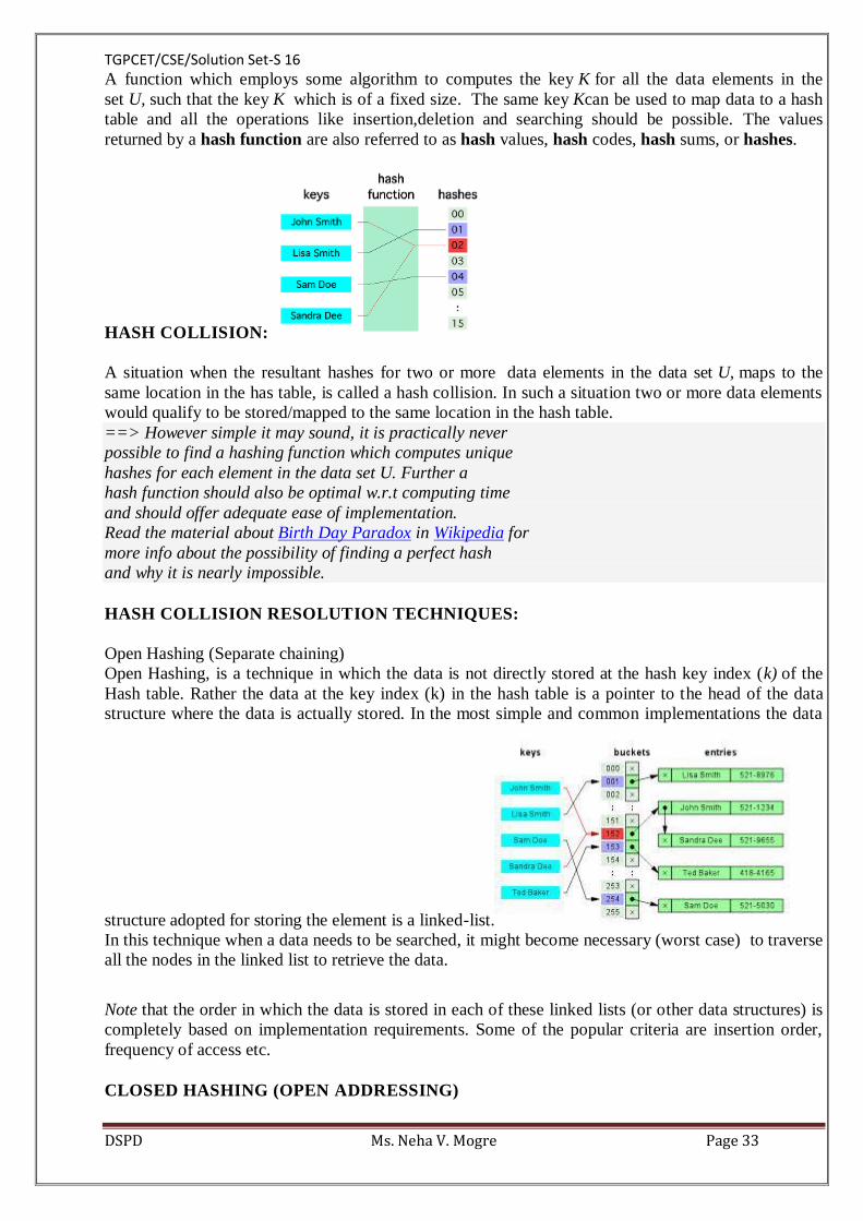
A function which employs some algorithm to computes the key K for all the data elements in the
set U, such that the key K which is of a fixed size. The same key Kcan be used to map data to a hash
table and all the operations like insertion,deletion and searching should be possible. The values
returned by a hash function are also referred to as hash values, hash codes, hash sums, or hashes.
HASH COLLISION:
A situation when the resultant hashes for two or more data elements in the data set U, maps to the
same location in the has table, is called a hash collision. In such a situation two or more data elements
would qualify to be stored/mapped to the same location in the hash table.
==> However simple it may sound, it is practically never
possible to find a hashing function which computes unique
hashes for each element in the data set U. Further a
hash function should also be optimal w.r.t computing time
and should offer adequate ease of implementation.
Read the material about Birth Day Paradox in Wikipedia for
more info about the possibility of finding a perfect hash
and why it is nearly impossible.
HASH COLLISION RESOLUTION TECHNIQUES:
Open Hashing (Separate chaining)
Open Hashing, is a technique in which the data is not directly stored at the hash key index (k) of the
Hash table. Rather the data at the key index (k) in the hash table is a pointer to the head of the data
structure where the data is actually stored. In the most simple and common implementations the data
structure adopted for storing the element is a linked-list.
In this technique when a data needs to be searched, it might become necessary (worst case) to traverse
all the nodes in the linked list to retrieve the data.
Note that the order in which the data is stored in each of these linked lists (or other data structures) is
completely based on implementation requirements. Some of the popular criteria are insertion order,
frequency of access etc.
CLOSED HASHING (OPEN ADDRESSING)

TGPCET/CSE/Solution Set-S 16
DSPD Ms. Neha V. Mogre Page 34
In this technique a hash table with pre-identified size is considered. All items are stored in the hash
table itself. In addition to the data, each hash bucket also maintains the three states: EMPTY,
OCCUPIED, DELETED. While inserting, if a collision occurs, alternative cells are tried until an
empty bucket is found. For which one of the following technique is adopted.
1. Liner Probing (this is prone to clustering of data + Some other constrains. Refer Wiki)
2. Quadratic probing (for more detail refer Wiki)
3. Double hashing (in short in case of collision another hashing function is used with the key
value as an input to identify where in the open addressing scheme the data should actually be
stored.)
A comparative analysis of Closed Hashing vs Open Hashing
Open Addressing Closed Addressing
All elements would be
stored in the Hash table
itself. No additional data
structure is needed.
Additional Data
structure needs to be
used to accommodate
collision data.
In cases of collisions, a
unique hash key must be
obtained.
Simple and effective
approach to collision
resolution. Key may or
may not be unique.
Determining size of the
hash table, adequate
enough for storing all
the data is difficult.
Performance
deterioration of closed
addressing much slower
as compared to Open
addressing.
State needs be
maintained for the data
(additional work)
No state data needs to be
maintained (easier to
maintain)
Uses space efficiently Expensive on space
12) Explain difference between static bee table and dynamic pee table
The key thing in hashing is to find an easy to compute hash function. However, collisions cannot be
avoided. Here we discuss three strategies of dealing with collisions, linear probing, quadratic probing
and separate chaining.
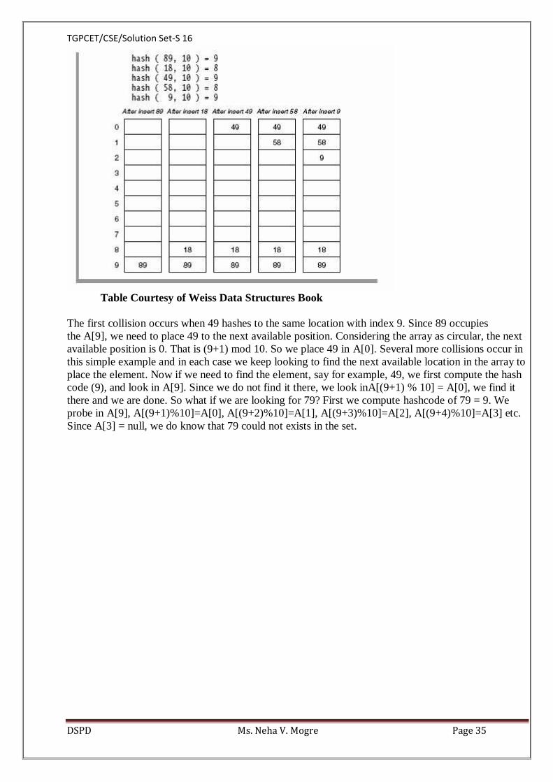
Linear Probing Suppose that a key hashes into a position that is already occupied. The simplest strategy is to look for
the next available position to place the item. Suppose we have a set of hash codes consisting of {89,
18, 49, 58, 9} and we need to place them into a table of size 10. The following table demonstrates this
process.
TGPCET/CSE/Solution Set-S 16
DSPD Ms. Neha V. Mogre Page 35
Table Courtesy of Weiss Data Structures Book
The first collision occurs when 49 hashes to the same location with index 9. Since 89 occupies
the A[9], we need to place 49 to the next available position. Considering the array as circular, the next
available position is 0. That is (9+1) mod 10. So we place 49 in A[0]. Several more collisions occur in
this simple example and in each case we keep looking to find the next available location in the array to
place the element. Now if we need to find the element, say for example, 49, we first compute the hash
code (9), and look in A[9]. Since we do not find it there, we look inA[(9+1) % 10] = A[0], we find it
there and we are done. So what if we are looking for 79? First we compute hashcode of 79 = 9. We
probe in A[9], A[(9+1)%10]=A[0], A[(9+2)%10]=A[1], A[(9+3)%10]=A[2], A[(9+4)%10]=A[3] etc.
Since A[3] = null, we do know that 79 could not exists in the set.
TGPCET/CSE/ Solution Set-S 17
DSPD Ms. Neha V. Mogre Page 1
Tulsiramji Gaikwad-Patil College of Engineering and Technology
Department of Computer Science and Engineering
Semester : B.E. Fourth Semester
Subject : DSPD
Solution Set: Summer – 2017
1a) Explain the various sorting techniques. Give its time complexities.
Bubble Sort [Best: O(n), Worst:O(N^2)]
Starting on the left, compare adjacent items and keep “bubbling” the larger one to the right (it’s in
its final place). Bubble sort the remaining N -1 items.
Though “simple” I found bubble sort nontrivial. In general, sorts where you iterate
backwards (decreasing some index) were counter-intuitive for me. With bubble-sort, either
you bubble items “forward” (left-to-right) and move the endpoint backwards (decreasing),
or bubble items “backward” (right-to-left) and increase the left endpoint. Either way, some
index is decreasing.
You also need to keep track of the next-to-last endpoint, so you don’t swap with a non-
existent item.
Selection Sort [Best/Worst: O(N^2)]
Scan all items and find the smallest. Swap it into position as the first item. Repeat the selection sort
on the remaining N-1 items.
I found this the most intuitive and easiest to implement — you always iterate forward (i
from 0 to N-1), and swap with the smallest element (always i).
Insertion Sort [Best: O(N), Worst:O(N^2)]
Start with a sorted list of 1 element on the left, and N-1 unsorted items on the right. Take the first
unsorted item (element #2) and insert it into the sorted list, moving elements as necessary. We now
have a sorted list of size 2, and N -2 unsorted elements. Repeat for all elements.
Like bubble sort, I found this counter-intuitive because you step “backwards”
This is a little like bubble sort for moving items, except when you encounter an item smaller
than you, you stop. If the data is reverse-sorted, each item must travel to the head of the list,
and this becomes bubble-sort.
There are various ways to move the item leftwards — you can do a swap on each iteration,
or copy each item over its neighbor
Radix sort [Best/Avg/Worst: O(N)]
Get a series of numbers, and sort them one digit at a time (moving all the 1000’s ahead of the
2000’s, etc.). Repeat the sorting on each set of digits.
Radix sort uses counting sort for efficient O(N) sorting of the digits (k = 0…9)
Actually, radix sort goes from least significant digit (1’s digit) to most significant, for
reasons I’ll explain later (see CLRS book)
TGPCET/CSE/ Solution Set-S 17
DSPD Ms. Neha V. Mogre Page 2
Radix & counting sort are fast, but require structured data, external memory and do not have
the caching benefits of quicksort.
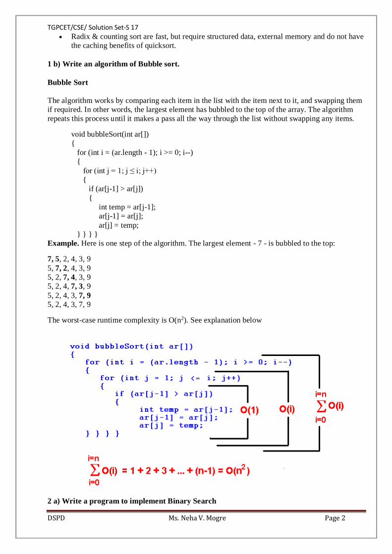
1 b) Write an algorithm of Bubble sort.
Bubble Sort
The algorithm works by comparing each item in the list with the item next to it, and swapping them
if required. In other words, the largest element has bubbled to the top of the array. The algorithm
repeats this process until it makes a pass all the way through the list without swapping any items.
void bubbleSort(int ar[])
{
for (int i = (ar.length - 1); i >= 0; i--)
{
for (int j = 1; j ≤ i; j++)
{
if (ar[j-1] > ar[j])
{
int temp = ar[j-1];
ar[j-1] = ar[j];
ar[j] = temp;
} } } }
Example. Here is one step of the algorithm. The largest element - 7 - is bubbled to the top:
7, 5, 2, 4, 3, 9
5, 7, 2, 4, 3, 9
5, 2, 7, 4, 3, 9
5, 2, 4, 7, 3, 9
5, 2, 4, 3, 7, 9
5, 2, 4, 3, 7, 9
The worst-case runtime complexity is O(n2). See explanation below
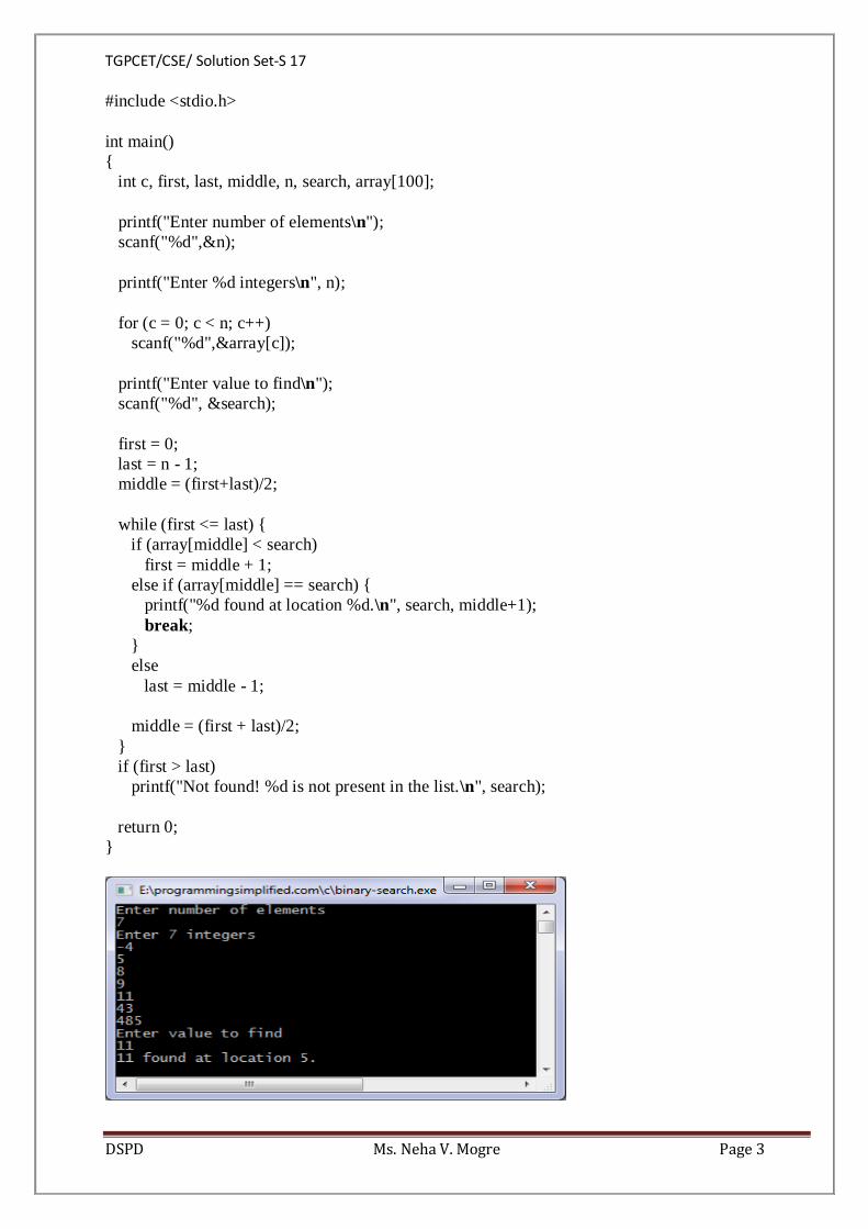
2 a) Write a program to implement Binary Search
TGPCET/CSE/ Solution Set-S 17
DSPD Ms. Neha V. Mogre Page 3
#include <stdio.h>
int main()
{
int c, first, last, middle, n, search, array[100];
printf("Enter number of elements\n");
scanf("%d",&n);
printf("Enter %d integers\n", n);
for (c = 0; c < n; c++)
scanf("%d",&array[c]);
printf("Enter value to find\n");
scanf("%d", &search);
first = 0;
last = n - 1;
middle = (first+last)/2;
while (first <= last) {
if (array[middle] < search)
first = middle + 1;
else if (array[middle] == search) {
printf("%d found at location %d.\n", search, middle+1);
break;
}
else
last = middle - 1;
middle = (first + last)/2;
}
if (first > last)
printf("Not found! %d is not present in the list.\n", search);
return 0;
}
TGPCET/CSE/ Solution Set-S 17
DSPD Ms. Neha V. Mogre Page 4
2b) Explain the following terms :––
i)Sparse Matrix.
What is Sparse Matrix?
In computer programming, a matrix can be defined with a 2-dimensional array. Any array with 'm'
columns and 'n' rows represents a mXn matrix. There may be a situation in which a matrix contains
more number of ZERO values than NON-ZERO values. Such matrix is known as sparse matrix.
Sparse matrix is a matrix which contains very few non-zero elements.
When a sparse matrix is represented with 2-dimensional array, we waste lot of space to represent
that matrix. For example, consider a matrix of size 100 X 100 containing only 10 non-zero
elements. In this matrix, only 10 spaces are filled with non-zero values and remaining spaces of
matrix are filled with zero. That means, totally we allocate 100 X 100 X 2 = 20000 bytes of space to
store this integer matrix. And to access these 10 non-zero elements we have to make scanning for
10000 times.
Sparse Matrix Representations
A sparse matrix can be represented by using TWO representations, those are as follows...
1. Triplet Representation
2. Linked Representation
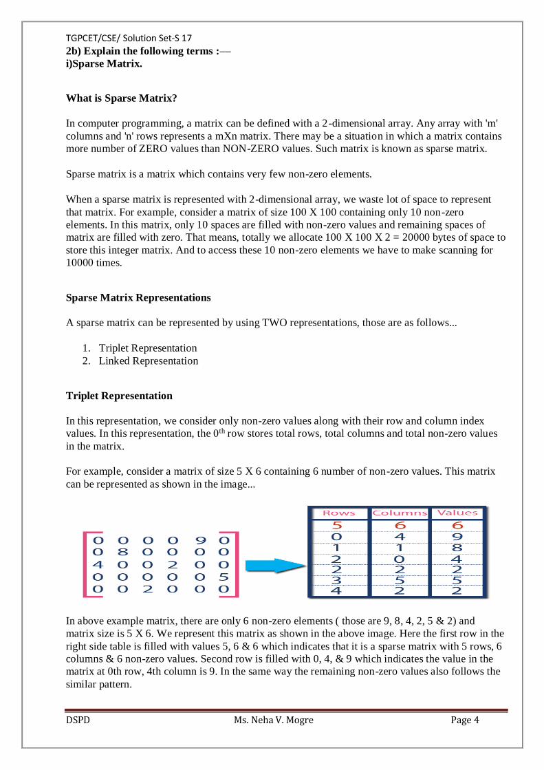
Triplet Representation
In this representation, we consider only non-zero values along with their row and column index
values. In this representation, the 0th row stores total rows, total columns and total non-zero values
in the matrix.
For example, consider a matrix of size 5 X 6 containing 6 number of non-zero values. This matrix
can be represented as shown in the image...
In above example matrix, there are only 6 non-zero elements ( those are 9, 8, 4, 2, 5 & 2) and
matrix size is 5 X 6. We represent this matrix as shown in the above image. Here the first row in the
right side table is filled with values 5, 6 & 6 which indicates that it is a sparse matrix with 5 rows, 6
columns & 6 non-zero values. Second row is filled with 0, 4, & 9 which indicates the value in the
matrix at 0th row, 4th column is 9. In the same way the remaining non-zero values also follows the
similar pattern.
TGPCET/CSE/ Solution Set-S 17
DSPD Ms. Neha V. Mogre Page 5
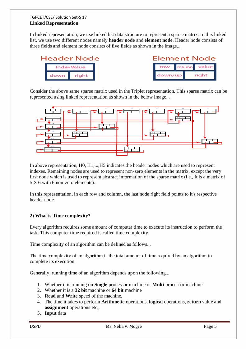
Linked Representation
In linked representation, we use linked list data structure to represent a sparse matrix. In this linked
list, we use two different nodes namely header node and element node. Header node consists of
three fields and element node consists of five fields as shown in the image...
Consider the above same sparse matrix used in the Triplet representation. This sparse matrix can be
represented using linked representation as shown in the below image...
In above representation, H0, H1,...,H5 indicates the header nodes which are used to represent
indexes. Remaining nodes are used to represent non-zero elements in the matrix, except the very
first node which is used to represent abstract information of the sparse matrix (i.e., It is a matrix of
5 X 6 with 6 non-zero elements).
In this representation, in each row and column, the last node right field points to it's respective
header node.
2) What is Time complexity?
Every algorithm requires some amount of computer time to execute its instruction to perform the
task. This computer time required is called time complexity.
Time complexity of an algorithm can be defined as follows...
The time complexity of an algorithm is the total amount of time required by an algorithm to
complete its execution.
Generally, running time of an algorithm depends upon the following...
1. Whether it is running on Single processor machine or Multi processor machine.
2. Whether it is a 32 bit machine or 64 bit machine
3. Read and Write speed of the machine.
4. The time it takes to perform Arithmetic operations, logical operations, return value and
assignment operations etc.,
5. Input data

TGPCET/CSE/ Solution Set-S 17
DSPD Ms. Neha V. Mogre Page 6
NOTE
☀ When we calculate time complexity of an algorithm, we consider only input data and ignore the
remaining things, as they are machine dependent. We check only, how our program is behaving for
the different input values to perform all the operations like Arithmetic, Logical, Return value and
Assignment etc.,
Calculating Time Complexity of an algorithm based on the system configuration is a very difficult
task because, the configuration changes from one system to another system. To solve this problem,
we must assume a model machine with specific configuration. So that, we can able to calculate
generalized time complexity according to that model machine.
To calculate time complexity of an algorithm, we need to define a model machine. Let us assume a
machine with following configuration...
1. Single processor machine
2. 32 bit Operating System machine
3. It performs sequential execution
4. It requires 1 unit of time for Arithmetic and Logical operations
5. It requires 1 unit of time for Assignment and Return value
6. It requires 1 unit of time for Read and Write operations
Now, we calculate the time complexity of following example code by using the above defined
model machine...
Example 1
Consider the following piece of code...
int sum(int a, int b)
{
return a+b;
}
In above sample code, it requires 1 unit of time to calculate a+b and 1 unit of time to return the
value. That means, totally it takes 2 units of time to complete its execution. And it does not change
based on the input values of a and b. That means for all input values, it requires same amount of
time i.e. 2 units.
If any program requires fixed amount of time for all input values then its time complexity is said to
be Constant Time Complexity.
For the above code, time complexity can be calculated as follows...
TGPCET/CSE/ Solution Set-S 17
DSPD Ms. Neha V. Mogre Page 7
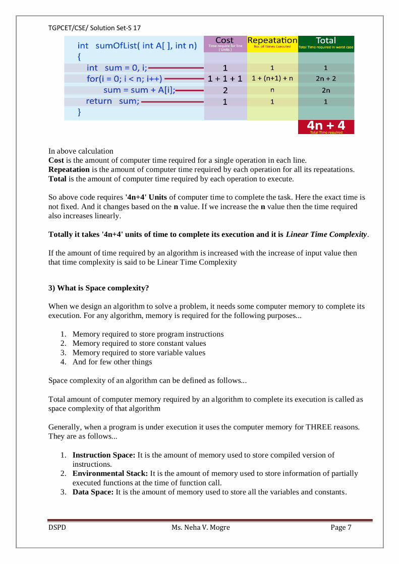
In above calculation
Cost is the amount of computer time required for a single operation in each line.
Repeatation is the amount of computer time required by each operation for all its repeatations.
Total is the amount of computer time required by each operation to execute.
So above code requires '4n+4' Units of computer time to complete the task. Here the exact time is
not fixed. And it changes based on the n value. If we increase the n value then the time required
also increases linearly.
Totally it takes '4n+4' units of time to complete its execution and it is Linear Time Complexity.
If the amount of time required by an algorithm is increased with the increase of input value then
that time complexity is said to be Linear Time Complexity
3) What is Space complexity?
When we design an algorithm to solve a problem, it needs some computer memory to complete its
execution. For any algorithm, memory is required for the following purposes...
1. Memory required to store program instructions
2. Memory required to store constant values
3. Memory required to store variable values
4. And for few other things
Space complexity of an algorithm can be defined as follows...
Total amount of computer memory required by an algorithm to complete its execution is called as
space complexity of that algorithm
Generally, when a program is under execution it uses the computer memory for THREE reasons.
They are as follows...
1. Instruction Space: It is the amount of memory used to store compiled version of
instructions.
2. Environmental Stack: It is the amount of memory used to store information of partially
executed functions at the time of function call.
3. Data Space: It is the amount of memory used to store all the variables and constants.

TGPCET/CSE/ Solution Set-S 17
DSPD Ms. Neha V. Mogre Page 8
NOTE
☀ When we want to perform analysis of an algorithm based on its Space complexity, we consider
only Data Space and ignore Instruction Space as well as Environmental Stack.
That means we calculate only the memory required to store Variables, Constants, Structures, etc.,
To calculate the space complexity, we must know the memory required to store different datatype
values (according to the compiler). For example, the C Programming Language compiler requires
the following...
1. 2 bytes to store Integer value,
2. 4 bytes to store Floating Point value,
3. 1 byte to store Character value,
4. 6 (OR) 8 bytes to store double value
Example 1
Consider the following piece of code...
int square(int a)
{
return a*a;
}
In above piece of code, it requires 2 bytes of memory to store variable 'a' and another 2 bytes of
memory is used for return value.
That means, totally it requires 4 bytes of memory to complete its execution. And this 4 bytes
of memory is fixed for any input value of 'a'. This space complexity is said to be Constant
Space Complexity.
If any algorithm requires a fixed amount of space for all input values then that space complexity is
said to be Constant Space Complexity
Example 2
Consider the following piece of code...
int sum(int A[], int n)
{
int sum = 0, i;
for(i = 0; i < n; i++)
sum = sum + A[i];
return sum;
}
In above piece of code it requires
TGPCET/CSE/ Solution Set-S 17
DSPD Ms. Neha V. Mogre Page 9
'n*2' bytes of memory to store array variable 'a[]'
2 bytes of memory for integer parameter 'n'
4 bytes of memory for local integer variables 'sum' and 'i' (2 bytes each)
2 bytes of memory for return value.
That means, totally it requires '2n+8' bytes of memory to complete its execution. Here, the
amount of memory depends on the input value of 'n'. This space complexity is said to be
Linear Space Complexity.
If the amount of space required by an algorithm is increased with the increase of input value, then
that space complexity is said to be Linear Space Complexity
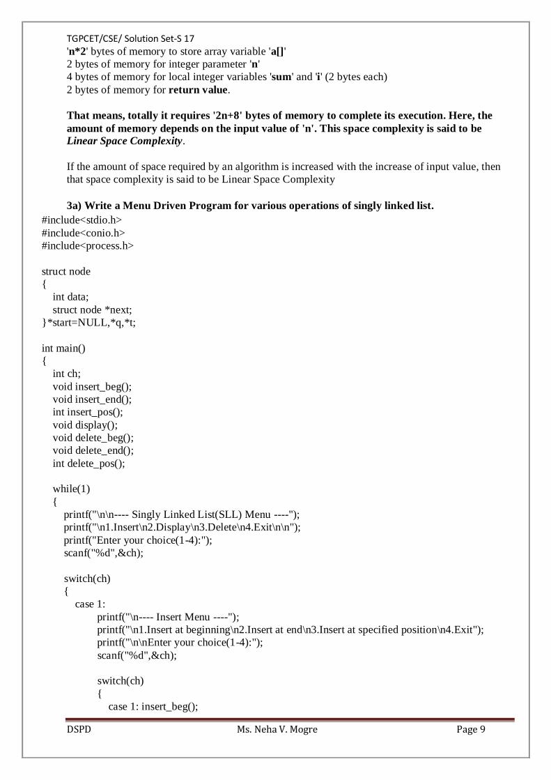
3a) Write a Menu Driven Program for various operations of singly linked list.
#include<stdio.h>
#include<conio.h>
#include<process.h>
struct node
{
int data;
struct node *next;
}*start=NULL,*q,*t;
int main()
{
int ch;
void insert_beg();
void insert_end();
int insert_pos();
void display();
void delete_beg();
void delete_end();
int delete_pos();
while(1)
{
printf("\n\n---- Singly Linked List(SLL) Menu ----");
printf("\n1.Insert\n2.Display\n3.Delete\n4.Exit\n\n");
printf("Enter your choice(1-4):");
scanf("%d",&ch);
switch(ch)
{
case 1:
printf("\n---- Insert Menu ----");
printf("\n1.Insert at beginning\n2.Insert at end\n3.Insert at specified position\n4.Exit");
printf("\n\nEnter your choice(1-4):");
scanf("%d",&ch);
switch(ch)
{
case 1: insert_beg();

TGPCET/CSE/ Solution Set-S 17
DSPD Ms. Neha V. Mogre Page 10
break;
case 2: insert_end();
break;
case 3: insert_pos();
break;
case 4: exit(0);
default: printf("Wrong Choice!!");
}
break;
case 2: display();
break;
case 3: printf("\n---- Delete Menu ----");
printf("\n1.Delete from beginning\n2.Delete from end\n3.Delete from specified
position\n4.Exit");
printf("\n\nEnter your choice(1-4):");
scanf("%d",&ch);
switch(ch)
{
case 1: delete_beg();
break;
case 2: delete_end();
break;
case 3: delete_pos();
break;
case 4: exit(0);
default: printf("Wrong Choice!!");
}
break;
case 4: exit(0);
default: printf("Wrong Choice!!");
}
}
return 0;
}
void insert_beg()
{
int num;
t=(struct node*)malloc(sizeof(struct node));
printf("Enter data:");
scanf("%d",&num);
t->data=num;
if(start==NULL) //If list is empty
{
t->next=NULL;
start=t;
}
else
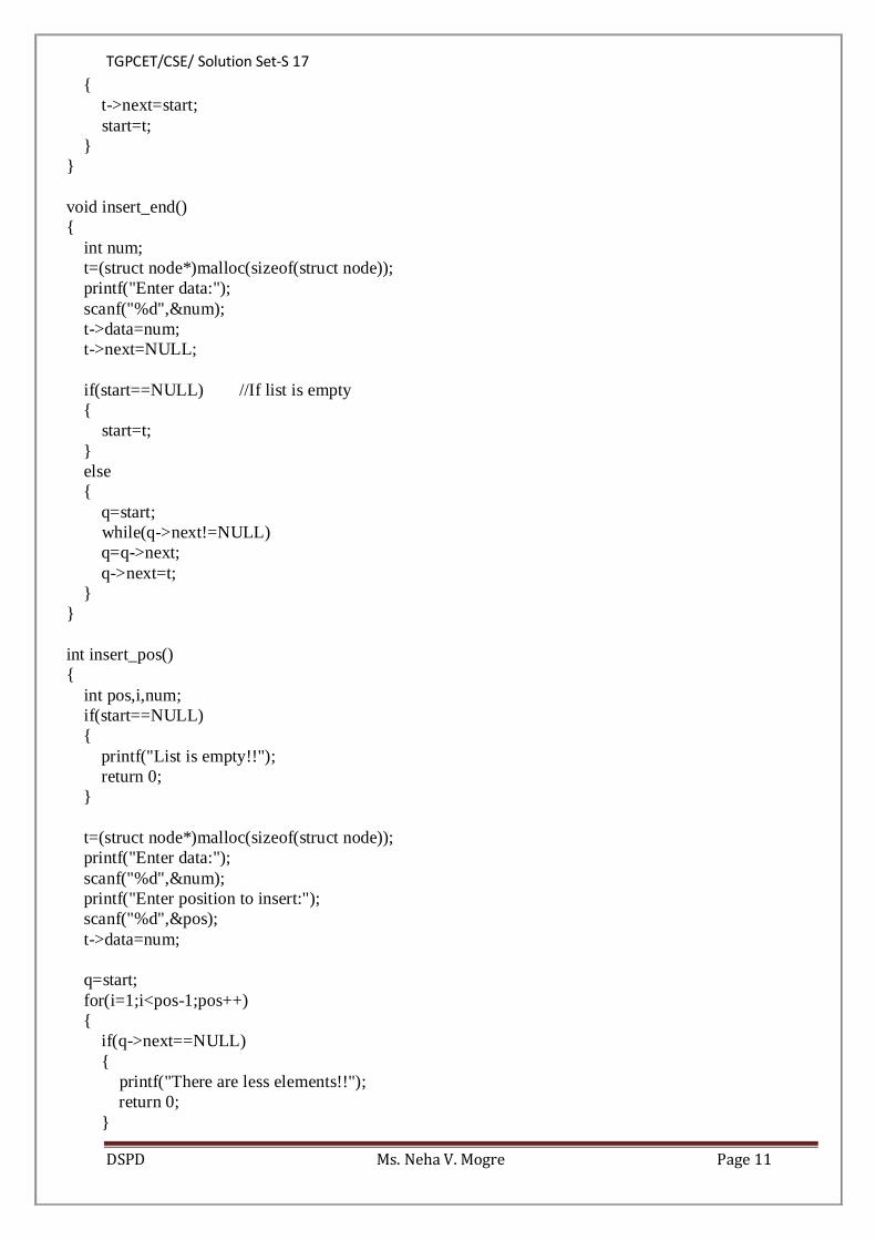
TGPCET/CSE/ Solution Set-S 17
DSPD Ms. Neha V. Mogre Page 11
{
t->next=start;
start=t;
}
}
void insert_end()
{
int num;
t=(struct node*)malloc(sizeof(struct node));
printf("Enter data:");
scanf("%d",&num);
t->data=num;
t->next=NULL;
if(start==NULL) //If list is empty
{
start=t;
}
else
{
q=start;
while(q->next!=NULL)
q=q->next;
q->next=t;
}
}
int insert_pos()
{
int pos,i,num;
if(start==NULL)
{
printf("List is empty!!");
return 0;
}
t=(struct node*)malloc(sizeof(struct node));
printf("Enter data:");
scanf("%d",&num);
printf("Enter position to insert:");
scanf("%d",&pos);
t->data=num;
q=start;
for(i=1;i<pos-1;pos++)
{
if(q->next==NULL)
{
printf("There are less elements!!");
return 0;
}
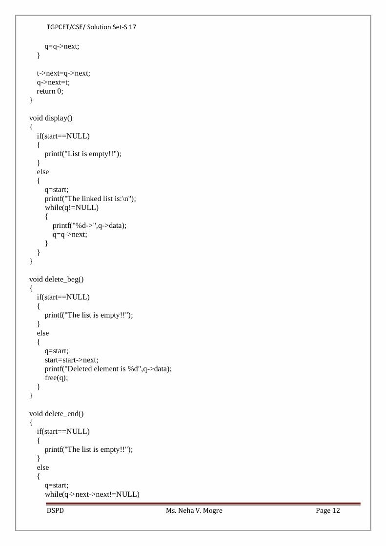
TGPCET/CSE/ Solution Set-S 17
DSPD Ms. Neha V. Mogre Page 12
q=q->next;
}
t->next=q->next;
q->next=t;
return 0;
}
void display()
{
if(start==NULL)
{
printf("List is empty!!");
}
else
{
q=start;
printf("The linked list is:\n");
while(q!=NULL)
{
printf("%d->",q->data);
q=q->next;
}
}
}
void delete_beg()
{
if(start==NULL)
{
printf("The list is empty!!");
}
else
{
q=start;
start=start->next;
printf("Deleted element is %d",q->data);
free(q);
}
}
void delete_end()
{
if(start==NULL)
{
printf("The list is empty!!");
}
else
{
q=start;
while(q->next->next!=NULL)

TGPCET/CSE/ Solution Set-S 17
DSPD Ms. Neha V. Mogre Page 13
q=q->next;
t=q->next;
q->next=NULL;
printf("Deleted element is %d",t->data);
free(t);
}
}
int delete_pos()
{
int pos,i;
if(start==NULL)
{
printf("List is empty!!");
return 0;
}
printf("Enter position to delete:");
scanf("%d",&pos);
for(i=1;i<pos-1;pos++)
{
if(q->next==NULL)
{
printf("There are less elements!!");
return 0;
}
q=q->next;
}
t=q->next;
q->next=t->next;
printf("Deleted element is %d",t->data);
free(t);
return 0;
}
Output —- Singly Linked List(SLL) Menu —-
1.Insert
2.Display
3.Delete
4.ExitEnter your choice(1-4):1—- Insert Menu —-
1.Insert at beginning
2.Insert at end
3.Insert at specified position
4.Exit
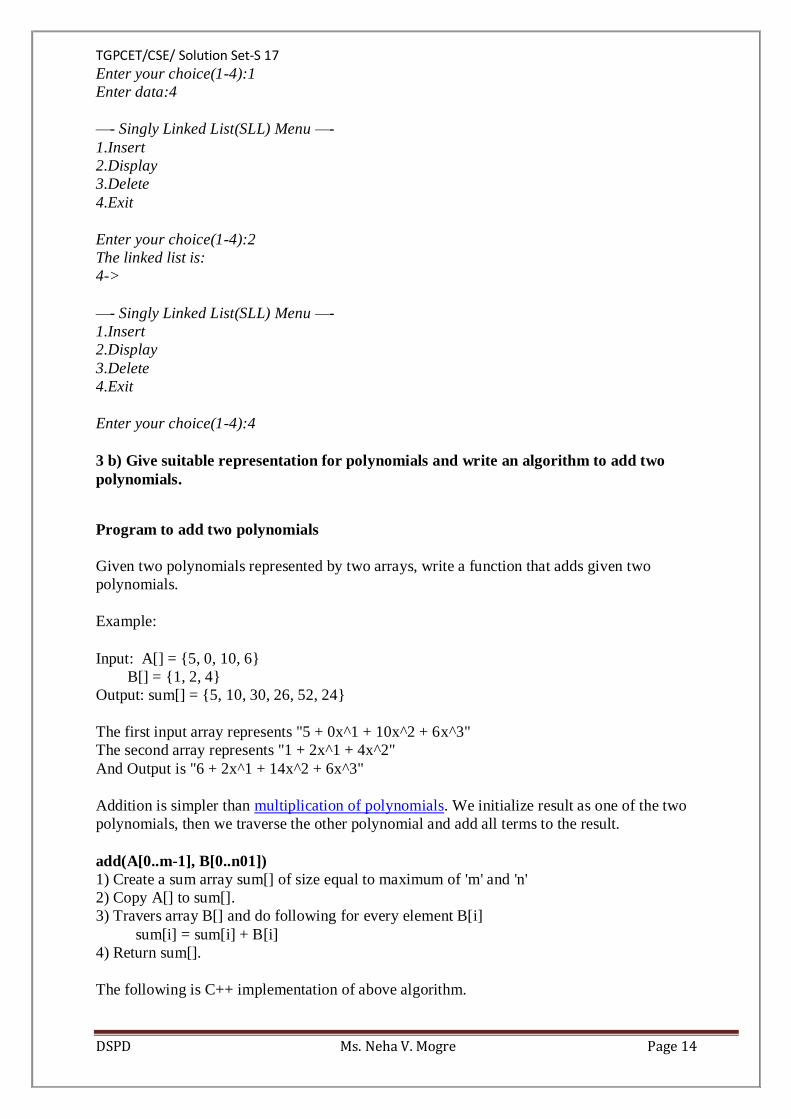
TGPCET/CSE/ Solution Set-S 17
DSPD Ms. Neha V. Mogre Page 14
Enter your choice(1-4):1
Enter data:4
—- Singly Linked List(SLL) Menu —-
1.Insert
2.Display
3.Delete
4.Exit
Enter your choice(1-4):2
The linked list is:
4->
—- Singly Linked List(SLL) Menu —-
1.Insert
2.Display
3.Delete
4.Exit
Enter your choice(1-4):4
3 b) Give suitable representation for polynomials and write an algorithm to add two
polynomials.
Program to add two polynomials
Given two polynomials represented by two arrays, write a function that adds given two
polynomials.
Example:
Input: A[] = {5, 0, 10, 6}
B[] = {1, 2, 4}
Output: sum[] = {5, 10, 30, 26, 52, 24}
The first input array represents "5 + 0x^1 + 10x^2 + 6x^3"
The second array represents "1 + 2x^1 + 4x^2"
And Output is "6 + 2x^1 + 14x^2 + 6x^3"
Addition is simpler than multiplication of polynomials. We initialize result as one of the two
polynomials, then we traverse the other polynomial and add all terms to the result.
add(A[0..m-1], B[0..n01])
1) Create a sum array sum[] of size equal to maximum of 'm' and 'n'
2) Copy A[] to sum[].
3) Travers array B[] and do following for every element B[i]
sum[i] = sum[i] + B[i]
4) Return sum[].
The following is C++ implementation of above algorithm.
TGPCET/CSE/ Solution Set-S 17
DSPD Ms. Neha V. Mogre Page 15
// Simple C++ program to add two polynomials
#include <iostream>
using namespace std;
// A utility function to return maximum of two integers
int max(int m, int n) { return (m > n)? m: n; }
// A[] represents coefficients of first polynomial
// B[] represents coefficients of second polynomial
// m and n are sizes of A[] and B[] respectively
int *add(int A[], int B[], int m, int n)
{
int size = max(m, n);
int *sum = new int[size];
// Initialize the porduct polynomial
for (int i = 0; i<m; i++)
sum[i] = A[i];
// Take ever term of first polynomial
for (int i=0; i<n; i++)
sum[i] += B[i];
return sum;
}
// A utility function to print a polynomial
void printPoly(int poly[], int n)
{
for (int i=0; i<n; i++)

TGPCET/CSE/ Solution Set-S 17
DSPD Ms. Neha V. Mogre Page 16
{
cout << poly[i];
if (i != 0)
cout << "x^" << i ;
if (i != n-1)
cout << " + ";
}
}
// Driver program to test above functions
int main()
{
// The following array represents polynomial 5 + 10x^2 + 6x^3
int A[] = {5, 0, 10, 6};
// The following array represents polynomial 1 + 2x + 4x^2
int B[] = {1, 2, 4};
int m = sizeof(A)/sizeof(A[0]);
int n = sizeof(B)/sizeof(B[0]);
cout << "First polynomial is \n";
printPoly(A, m);
cout << "\nSecond polynomial is \n";
printPoly(B, n);
int *sum = add(A, B, m, n);
int size = max(m, n);
cout << "\nsumuct polynomial is \n";
printPoly(sum, size);
TGPCET/CSE/ Solution Set-S 17
DSPD Ms. Neha V. Mogre Page 17
return 0;
}
Output:
First polynomial is
5 + 0x^1 + 10x^2 + 6x^3
Second polynomial is
1 + 2x^1 + 4x^2
Sum polynomial is
6 + 2x^1 + 14x^2 + 6x^3
Time complexity of the above algorithm and program is O(m+n) where m and n are orders of two
given polynomials.
4) Write a function to :––
(i) Insert a node at end in doubly linked list
Insertion At Last in doubly linked list
Algorithm
1. InsertAtEndDll(info,prev,next,start,end)
2. 1.create a new node and address in assigned to ptr.
3. 2.check[overflow] if(ptr=NULL)
4. write:overflow and exit
5. 3.set Info[ptr]=item;
6. 4.if(start=NULL)
7. set prev[ptr] = next[ptr] = NULL
8. set start = end = ptr
9. else
10. set prev[ptr] = end
11. next[end] = ptr
12. set ptr[next] = NULL
13. set end = ptr
14. [end if]
15. 5.Exit.
b)Delete a node from a specific position from doubly linked list.
Algorithm to delete node from any position of a doubly linked list
Algorithm to delete node from any position %% Input : head {Pointer to the first node of the list}

TGPCET/CSE/ Solution Set-S 17
DSPD Ms. Neha V. Mogre Page 18
last {Pointer to the last node of the list}
N {Position to be deleted from list}
Begin:
current ← head;
For i ← 1 to N and current != NULL do
current ← current.next;
End for If (N == 1) then
deleteFromBeginning()
End if Else if (current == last) then
deleteFromEnd()
End if Else if (current != NULL) then
current.prev.next ← current.next
If (current.next != NULL) then
current.next.prev ← current.prev;
End if
unalloc (current)
write ('Node deleted successfully from ', N, ' position')
End if
Else then
write ('Invalid position')
End if
End
4b) What is static memory allocation and dynamic memory allocation ? What are the
functions used for dynamic memory allocation in ''C'' ? Give examples.
static memory allocation and dynamic memory allocation:-
Static Memory Allocation: Memory is allocated for the declared variable by the compiler. The
address can be obtained by using ‘address of’ operator and can be assigned to a pointer. The
memory is allocated during compile time. Since most of the declared variables have static memory,
this kind of assigning the address of a variable to a pointer is known as static memory allocation.
Dynamic Memory Allocation: Allocation of memory at the time of execution (run time) is known
as dynamic memory allocation. The functions calloc() and malloc() support allocating of dynamic
memory. Dynamic allocation of memory space is done by using these functions when value is
returned by functions and assigned to pointer variables.
In C, the exact size of array is unknown until compile time, i.e., the time when a compiler compiles
your code into a computer understandable language. So, sometimes the size of the array can be
insufficient or more than required.
Dynamic memory allocation allows your program to obtain more memory space while running, or
to release it if it's not required.
In simple terms, Dynamic memory allocation allows you to manually handle memory space for
your program.
TGPCET/CSE/ Solution Set-S 17
DSPD Ms. Neha V. Mogre Page 19
Although, C language inherently does not have any technique to allocate memory dynamically,
there are 4 library functions under "stdlib.h" for dynamic memory allocation.
Function Use of Function
malloc() Allocates requested size of bytes and returns a pointer first byte of allocated space
calloc()
Allocates space for an array elements, initializes to zero and then returns a pointer to
memory
free() deallocate the previously allocated space
realloc() Change the size of previously allocated space
C malloc()
The name malloc stands for "memory allocation".
The function malloc() reserves a block of memory of specified size and return a pointer of type void
which can be casted into pointer of any form.
Syntax of malloc()
ptr = (cast-type*) malloc(byte-size)
Here, ptr is pointer of cast-type. The malloc() function returns a pointer to an area of memory with
size of byte size. If the space is insufficient, allocation fails and returns NULL pointer.
ptr = (int*) malloc(100 * sizeof(int));
This statement will allocate either 200 or 400 according to size of int 2 or 4 bytes respectively and
the pointer points to the address of first byte of memory.
C calloc()
The name calloc stands for "contiguous allocation".
The only difference between malloc() and calloc() is that, malloc() allocates single block of
memory whereas calloc() allocates multiple blocks of memory each of same size and sets all bytes
to zero.
Syntax of calloc()
ptr = (cast-type*)calloc(n, element-size);
This statement will allocate contiguous space in memory for an array of n elements. For example:
ptr = (float*) calloc(25, sizeof(float));
This statement allocates contiguous space in memory for an array of 25 elements each of size of
float, i.e, 4 bytes.
TGPCET/CSE/ Solution Set-S 17
DSPD Ms. Neha V. Mogre Page 20
C free()
Dynamically allocated memory created with either calloc() or malloc() doesn't get freed on its own.
You must explicitly use free() to release the space.
syntax of free()
free(ptr);
This statement frees the space allocated in the memory pointed by ptr.
5a) Write an algorithm which convert infix expression into postfix from using stack and give
steps of each.
nfix to Postfix Conversion
Procedure for Postfix Conversion
1. Scan the Infix string from left to right.
2. Initialize an empty stack.
3. If the scanned character is an operand, add it to the Postfix string.
4. If the scanned character is an operator and if the stack is empty push the character to stack.
5. If the scanned character is an Operator and the stack is not empty, compare the precedence of
the character with the element on top of the stack.
6.
If top Stack has higher precedence over the scanned character pop the stack else push the
scanned character to stack. Repeat this step until the stack is not empty and top Stack has
precedence over the character.
7. Repeat 4 and 5 steps till all the characters are scanned.
8. After all characters are scanned, we have to add any character that the stack may have to the
Postfix string.
9. If stack is not empty add top Stack to Postfix string and Pop the stack.
10. Repeat this step as long as stack is not empty.
Algorithm for Postfix Conversion
1. S:stack
2. while(more tokens)
3. x<=next token
4. if(x == operand)
5. print x
6. else
7. while(precedence(x)<=precedence(top(s)))
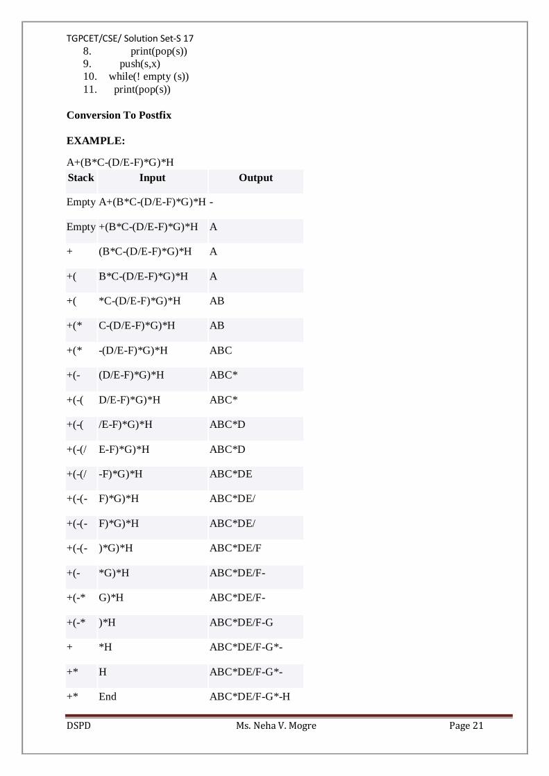
TGPCET/CSE/ Solution Set-S 17
DSPD Ms. Neha V. Mogre Page 21
8. print(pop(s))
9. push(s,x)
10. while(! empty (s))
11. print(pop(s))
Conversion To Postfix
EXAMPLE:
A+(B*C-(D/E-F)*G)*H
Stack Input Output
Empty A+(B*C-(D/E-F)*G)*H -
Empty +(B*C-(D/E-F)*G)*H A
+ (B*C-(D/E-F)*G)*H A
+( B*C-(D/E-F)*G)*H A
+( *C-(D/E-F)*G)*H AB
+(* C-(D/E-F)*G)*H AB
+(* -(D/E-F)*G)*H ABC
+(- (D/E-F)*G)*H ABC*
+(-( D/E-F)*G)*H ABC*
+(-( /E-F)*G)*H ABC*D
+(-(/ E-F)*G)*H ABC*D
+(-(/ -F)*G)*H ABC*DE
+(-(- F)*G)*H ABC*DE/
+(-(- F)*G)*H ABC*DE/
+(-(- )*G)*H ABC*DE/F
+(- *G)*H ABC*DE/F-
+(-* G)*H ABC*DE/F-
+(-* )*H ABC*DE/F-G
+ *H ABC*DE/F-G*-
+* H ABC*DE/F-G*-
+* End ABC*DE/F-G*-H
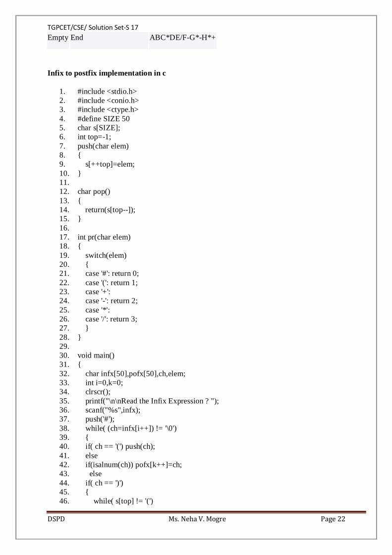
TGPCET/CSE/ Solution Set-S 17
DSPD Ms. Neha V. Mogre Page 22
Empty End ABC*DE/F-G*-H*+
Infix to postfix implementation in c
1. #include <stdio.h>
2. #include <conio.h>
3. #include <ctype.h>
4. #define SIZE 50
5. char s[SIZE];
6. int top=-1;
7. push(char elem)
8. {
9. s[++top]=elem;
10. }
11.
12. char pop()
13. {
14. return(s[top--]);
15. }
16.
17. int pr(char elem)
18. {
19. switch(elem)
20. {
21. case '#': return 0;
22. case '(': return 1;
23. case '+':
24. case '-': return 2;
25. case '*':
26. case '/': return 3;
27. }
28. }
29.
30. void main()
31. {
32. char infx[50],pofx[50],ch,elem;
33. int i=0,k=0;
34. clrscr();
35. printf("\n\nRead the Infix Expression ? ");
36. scanf("%s",infx);
37. push('#');
38. while( (ch=infx[i++]) != '\0')
39. {
40. if( ch == '(') push(ch);
41. else
42. if(isalnum(ch)) pofx[k++]=ch;
43. else
44. if( ch == ')')
45. {
46. while( s[top] != '(')
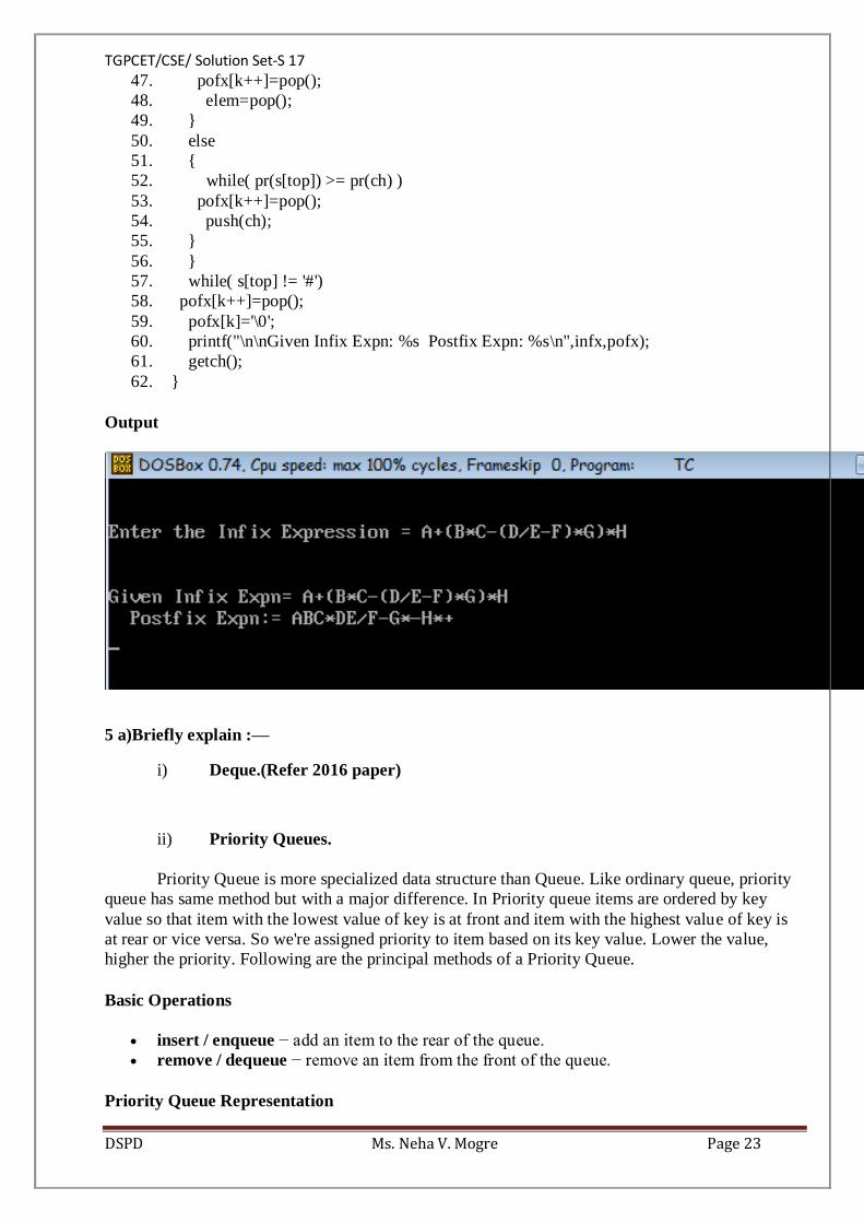
TGPCET/CSE/ Solution Set-S 17
DSPD Ms. Neha V. Mogre Page 23
47. pofx[k++]=pop();
48. elem=pop();
49. }
50. else
51. {
52. while( pr(s[top]) >= pr(ch) )
53. pofx[k++]=pop();
54. push(ch);
55. }
56. }
57. while( s[top] != '#')
58. pofx[k++]=pop();
59. pofx[k]='\0';
60. printf("\n\nGiven Infix Expn: %s Postfix Expn: %s\n",infx,pofx);
61. getch();
62. }
Output
5 a)Briefly explain :––
i) Deque.(Refer 2016 paper)
ii) Priority Queues.
Priority Queue is more specialized data structure than Queue. Like ordinary queue, priority
queue has same method but with a major difference. In Priority queue items are ordered by key
value so that item with the lowest value of key is at front and item with the highest value of key is
at rear or vice versa. So we're assigned priority to item based on its key value. Lower the value,
higher the priority. Following are the principal methods of a Priority Queue.
Basic Operations
insert / enqueue − add an item to the rear of the queue.
remove / dequeue − remove an item from the front of the queue.
Priority Queue Representation

TGPCET/CSE/ Solution Set-S 17
DSPD Ms. Neha V. Mogre Page 24
We're going to implement Queue using array in this article. There is few more operations supported
by queue which are following.
Peek − get the element at front of the queue.
isFull − check if queue is full.
isEmpty − check if queue is empty.
Insert / Enqueue Operation
Whenever an element is inserted into queue, priority queue inserts the item according to its order.
Here we're assuming that data with high value has low priority.
6a) What do you mean by circular queues ? Give the array implementation of it and write an
algorithm for insertion and deletion of elements from circular queues.
Circular Queue
In a normal Queue Data Structure, we can insert elements until queue becomes full. But once if
queue becomes full, we can not insert the next element until all the elements are deleted from the
queue. For example consider the queue below...
After inserting all the elements into the queue.
Now consider the following situation after deleting three elements from the queue...

TGPCET/CSE/ Solution Set-S 17
DSPD Ms. Neha V. Mogre Page 25
This situation also says that Queue is Full and we can not insert the new element because, 'rear' is
still at last position. In above situation, even though we have empty positions in the queue we can
not make use of them to insert new element. This is the major problem in normal queue data
structure. To overcome this problem we use circular queue data structure.
Implementation of Circular Queue
To implement a circular queue data structure using array, we first perform the following steps
before we implement actual operations.
Step 1: Include all the header files which are used in the program and define a constant
'SIZE' with specific value.
Step 2: Declare all user defined functions used in circular queue implementation.
Step 3: Create a one dimensional array with above defined SIZE (int cQueue[SIZE])
Step 4: Define two integer variables 'front' and 'rear' and initialize both with '-1'. (int
front = -1, rear = -1)
Step 5: Implement main method by displaying menu of operations list and make suitable
function calls to perform operation selected by the user on circular queue.
enQueue(value) - Inserting value into the Circular Queue
In a circular queue, enQueue() is a function which is used to insert an element into the circular
queue. In a circular queue, the new element is always inserted at rear position. The enQueue()
function takes one integer value as parameter and inserts that value into the circular queue. We can
use the following steps to insert an element into the circular queue...
Step 1: Check whether queue is FULL. ((rear == SIZE-1 && front == 0) || (front ==
rear+1))
Step 2: If it is FULL, then display "Queue is FULL!!! Insertion is not possible!!!" and
terminate the function.
Step 3: If it is NOT FULL, then check rear == SIZE - 1 && front != 0 if it is TRUE,
then set rear = -1.
Step 4: Increment rear value by one (rear++), set queue[rear] = value and check 'front ==
-1' if it is TRUE, then set front = 0.
deQueue() - Deleting a value from the Circular Queue
In a circular queue, deQueue() is a function used to delete an element from the circular queue. In a
circular queue, the element is always deleted from front position. The deQueue() function doesn't
take any value as parameter. We can use the following steps to delete an element from the circular
queue...
Step 1: Check whether queue is EMPTY. (front == -1 && rear == -1)

TGPCET/CSE/ Solution Set-S 17
DSPD Ms. Neha V. Mogre Page 26
Step 2: If it is EMPTY, then display "Queue is EMPTY!!! Deletion is not possible!!!"
and terminate the function.
Step 3: If it is NOT EMPTY, then display queue[front] as deleted element and increment
the front value by one (front ++). Then check whether front == SIZE, if it is TRUE, then
set front = 0. Then check whether both front - 1 and rear are equal (front -1 == rear), if it
TRUE, then set both front and rear to '-1' (front = rear = -1).
display() - Displays the elements of a Circular Queue
We can use the following steps to display the elements of a circular queue...
Step 1: Check whether queue is EMPTY. (front == -1)
Step 2: If it is EMPTY, then display "Queue is EMPTY!!!" and terminate the function.
Step 3: If it is NOT EMPTY, then define an integer variable 'i' and set 'i = front'.
Step 4: Check whether 'front <= rear', if it is TRUE, then display 'queue[i]' value and
increment 'i' value by one (i++). Repeat the same until 'i <= rear' becomes FALSE.
Step 5: If 'front <= rear' is FALSE, then display 'queue[i]' value and increment 'i' value by
one (i++). Repeat the same until'i <= SIZE - 1' becomes FALSE.
Step 6: Set i to 0.
Step 7: Again display 'cQueue[i]' value and increment i value by one (i++). Repeat the
same until 'i <= rear' becomes FALSE.
Program to implement Queue using Array
#include<stdio.h>
#include<conio.h>
#define SIZE 5
void enQueue(int);
void deQueue();
void display();
int cQueue[SIZE], front = -1, rear = -1;
void main()
{
int choice, value;
clrscr();
while(1){
printf("\n****** MENU ******\n");
printf("1. Insert\n2. Delete\n3. Display\n4. Exit\n");
printf("Enter your choice: ");
scanf("%d",&choice);
switch(choice){
case 1: printf("\nEnter the value to be insert: ");
scanf("%d",&value);
enQueue(value);
break;
case 2: deQueue();
break;
case 3: display();
break;

TGPCET/CSE/ Solution Set-S 17
DSPD Ms. Neha V. Mogre Page 27
case 4: exit(0);
default: printf("\nPlease select the correct choice!!!\n");
}
}
}
void enQueue(int value)
{
if((front == 0 && rear == SIZE - 1) || (front == rear+1))
printf("\nCircular Queue is Full! Insertion not possible!!!\n");
else{
if(rear == SIZE-1 && front != 0)
rear = -1;
cQueue[++rear] = value;
printf("\nInsertion Success!!!\n");
if(front == -1)
front = 0;
}
}
void deQueue()
{
if(front == -1 && rear == -1)
printf("\nCircular Queue is Empty! Deletion is not possible!!!\n");
else{
printf("\nDeleted element : %d\n",cQueue[front++]);
if(front == SIZE)
front = 0;
if(front-1 == rear)
front = rear = -1;
}
}
void display()
{
if(front == -1)
printf("\nCircular Queue is Empty!!!\n");
else{
int i = front;
printf("\nCircular Queue Elements are : \n");
if(front <= rear){
while(i <= rear)
printf("%d\t",cQueue[i++]);
}
else{
while(i <= SIZE - 1)
printf("%d\t", cQueue[i++]);
i = 0;
while(i <= rear)
printf("%d\t",cQueue[i++]);
}
}
}

TGPCET/CSE/ Solution Set-S 17
DSPD Ms. Neha V. Mogre Page 28
Output
7) Explain the terms :––
i) Polish Notations
The name comes from the Polish mathematician/logician Lukasiewicz, who introduced it. Three
types:
Infix form
Prefix form
Postfix form
TGPCET/CSE/ Solution Set-S 17
DSPD Ms. Neha V. Mogre Page 29
Infix form
Is exactly the fully parenthesized notation we have just introduced. Let me remind you once again
the Recursive definition
infix-expression := (infix-expression operand infix-expression)
infix-expression := atom
Examples
(3 * 7)
((1 + 3) * 2)
((1 + 3) * ( 2 - 3))
Main Feature: the binary operator is between the two operands.
Question: what if we do not put all the parentheses? Then there are ambiguities on how to interpret
an expression: is 1+2*3 the same as (1+2)*3 or the same as 1+(2*3)? The precedence of operators
solves this problem.
Prefix form
Main Feature: the operator preceeds the two operands.
Recursive definition of fully parenthesized version:
prefix-expression := (operand prefix-expression prefix-expression)
prefix-expression := atom
Recursive definition of classic version, without parentheses (we do not need them, because there is
no longer any ambiguity on how to match the operands to the operators):
prefix-expression := operand prefix-expression prefix-expression
prefix-expression := atom
Examples
(* 3 7) or simply * 3 7
(* ( + 1 3) 2) or simply * + 1 3 2
( * ( + 1 3) ( - 2 3)) or simply * + 1 3 - 2 3
Postfix form
Main Feature: the operator is after the two operands. Recursive definition
postfix-expression := (operand postfix-expression postfix-expression)
postfix-expression := atom

TGPCET/CSE/ Solution Set-S 17
DSPD Ms. Neha V. Mogre Page 30
Recursive definition of classic version, without parentheses (we do not need them, because there is
no longer any ambiguity on how to match the operands to the operators):
postfix-expression := operand postfix-expression postfix-expression
postfix-expression := atom
Examples
(3 7 *) or simply 3 7 *
((1 3 + ) 2 *) or simply 1 3 + 2 *
((1 3 +) ( 2 3 -) * ) or simply 1 3 + 2 3 - *
b) Push and POP Algorithm.
A stack is an Abstract Data Type (ADT), commonly used in most programming languages. It is
named stack as it behaves like a real-world stack, for example – a deck of cards or a pile of plates,
etc.A real-world stack allows operations at one end only. For example, we can place or remove a
card or plate from the top of the stack only. Likewise, Stack ADT allows all data operations at one
end only. At any given time, we can only access the top element of a stack.
This feature makes it LIFO data structure. LIFO stands for Last-in-first-out. Here, the element
which is placed (inserted or added) last, is accessed first. In stack terminology, insertion operation
is called PUSH operation and removal operation is called POP operation.
Stack Representation
The following diagram depicts a stack and its operations −
A stack can be implemented by means of Array, Structure, Pointer, and Linked List. Stack can
either be a fixed size one or it may have a sense of dynamic resizing. Here, we are going to
implement stack using arrays, which makes it a fixed size stack implementation.
TGPCET/CSE/ Solution Set-S 17
DSPD Ms. Neha V. Mogre Page 31
Basic Operations
Stack operations may involve initializing the stack, using it and then de-initializing it. Apart from
these basic stuffs, a stack is used for the following two primary operations −
push() − Pushing (storing) an element on the stack.
pop() − Removing (accessing) an element from the stack.
When data is PUSHed onto stack.
To use a stack efficiently, we need to check the status of stack as well. For the same purpose, the
following functionality is added to stacks −
peek() − get the top data element of the stack, without removing it.
isFull() − check if stack is full.
isEmpty() − check if stack is empty.
At all times, we maintain a pointer to the last PUSHed data on the stack. As this pointer always
represents the top of the stack, hence named top. The top pointer provides top value of the stack
without actually removing it.
First we should learn about procedures to support stack functions −
peek()
Algorithm of peek() function −
begin procedure peek
return stack[top]
end procedure
Implementation of peek() function in C programming language −
Example
int peek() {
return stack[top];
}
isfull()
Algorithm of isfull() function −
begin procedure isfull
if top equals to MAXSIZE
return true
else
return false
endif

TGPCET/CSE/ Solution Set-S 17
DSPD Ms. Neha V. Mogre Page 32
end procedure
Implementation of isfull() function in C programming language −
Example
bool isfull() {
if(top == MAXSIZE)
return true;
else
return false;
}
isempty()
Algorithm of isempty() function −
begin procedure isempty
if top less than 1
return true
else
return false
endif
end procedure
Implementation of isempty() function in C programming language is slightly different. We initialize
top at -1, as the index in array starts from 0. So we check if the top is below zero or -1 to determine
if the stack is empty. Here's the code −
Example
bool isempty() {
if(top == -1)
return true;
else
return false;
}
Push Operation
The process of putting a new data element onto stack is known as a Push Operation. Push operation
involves a series of steps −
Step 1 − Checks if the stack is full.
Step 2 − If the stack is full, produces an error and exit.
Step 3 − If the stack is not full, increments top to point next empty space.
Step 4 − Adds data element to the stack location, where top is pointing.
Step 5 − Returns success.

TGPCET/CSE/ Solution Set-S 17
DSPD Ms. Neha V. Mogre Page 33
If the linked list is used to implement the stack, then in step 3, we need to allocate space
dynamically.
Algorithm for PUSH Operation
A simple algorithm for Push operation can be derived as follows −
begin procedure push: stack, data
if stack is full
return null
endif
top ← top + 1
stack[top] ← data
end procedure
Implementation of this algorithm in C, is very easy. See the following code −
Example
void push(int data) {
if(!isFull()) {
top = top + 1;
stack[top] = data;
} else {
printf("Could not insert data, Stack is full.\n");
}
}
Pop Operation
Accessing the content while removing it from the stack, is known as a Pop Operation. In an array
implementation of pop() operation, the data element is not actually removed, instead top is
decremented to a lower position in the stack to point to the next value. But in linked-list
implementation, pop() actually removes data element and deallocates memory space.

TGPCET/CSE/ Solution Set-S 17
DSPD Ms. Neha V. Mogre Page 34
A Pop operation may involve the following steps −
Step 1 − Checks if the stack is empty.
Step 2 − If the stack is empty, produces an error and exit.
Step 3 − If the stack is not empty, accesses the data element at which top is pointing.
Step 4 − Decreases the value of top by 1.
Step 5 − Returns success.
Algorithm for Pop Operation
A simple algorithm for Pop operation can be derived as follows −
begin procedure pop: stack
if stack is empty
return null
endif
data ← stack[top]
top ← top - 1
return data
end procedure
Implementation of this algorithm in C, is as follows −
Example
int pop(int data) {
if(!isempty()) {
data = stack[top];
top = top - 1;
return data;
} else {
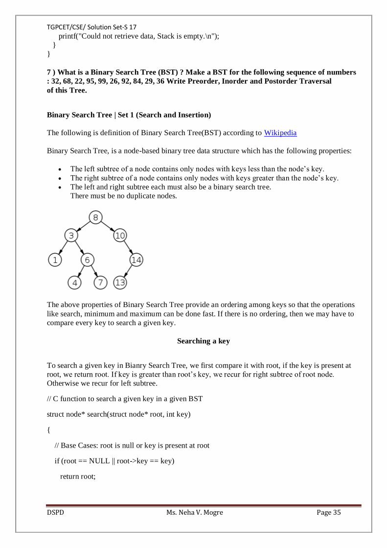
TGPCET/CSE/ Solution Set-S 17
DSPD Ms. Neha V. Mogre Page 35
printf("Could not retrieve data, Stack is empty.\n");
}
}
7 ) What is a Binary Search Tree (BST) ? Make a BST for the following sequence of numbers
: 32, 68, 22, 95, 99, 26, 92, 84, 29, 36 Write Preorder, Inorder and Postorder Traversal
of this Tree.
Binary Search Tree | Set 1 (Search and Insertion)
The following is definition of Binary Search Tree(BST) according to Wikipedia
Binary Search Tree, is a node-based binary tree data structure which has the following properties:
The left subtree of a node contains only nodes with keys less than the node’s key.
The right subtree of a node contains only nodes with keys greater than the node’s key.
The left and right subtree each must also be a binary search tree.
There must be no duplicate nodes.
The above properties of Binary Search Tree provide an ordering among keys so that the operations
like search, minimum and maximum can be done fast. If there is no ordering, then we may have to
compare every key to search a given key.
Searching a key
To search a given key in Bianry Search Tree, we first compare it with root, if the key is present at
root, we return root. If key is greater than root’s key, we recur for right subtree of root node.
Otherwise we recur for left subtree.
// C function to search a given key in a given BST
struct node* search(struct node* root, int key)
{
// Base Cases: root is null or key is present at root
if (root == NULL || root->key == key)
return root;

TGPCET/CSE/ Solution Set-S 17
DSPD Ms. Neha V. Mogre Page 36
// Key is greater than root's key
if (root->key < key)
return search(root->right, key);
// Key is smaller than root's key
return search(root->left, key);
}
Time Complexity: The worst case time complexity of search and insert operations is O(h) where h
is height of Binary Search Tree. In worst case, we may have to travel from root to the deepest leaf
node. The height of a skewed tree may become n and the time complexity of search and insert
operation may become O(n).
Some Interesting Facts:

TGPCET/CSE/ Solution Set-S 17
DSPD Ms. Neha V. Mogre Page 37
Inorder traversal of BST always produces sorted output.
We can construct a BST with only Preorder or Postorder or Level Order traversal. Note that
we can always get inorder traversal by sorting the only given traversal.
Number of unique BSTs with n distinct keys is Catalan Number
b) Explain the AVL Tree and Complete Binary Tree.
Ans:- Refer previous year solved solution paper.
8) What is threaded binary tree ?
Ans:- Refer previous year solved solution paper.
9) Write an algorithm for following (Any One) :–
i) BFS
(ii) DFS
Also discuss suitable example of it.
Ans:- Refer previous year solved solution paper.
10. (a) Define and explain following terminology of a graph as a data structure with example
:––
(i) Path and cycle.
A graph is a pictorial representation of a set of objects where some pairs of objects are connected by
links. The interconnected objects are represented by points termed as vertices, and the links that
connect the vertices are called edges.
Formally, a graph is a pair of sets (V, E), where V is the set of vertices and E is the set of edges,
connecting the pairs of vertices. Take a look at the following graph −
In the above graph,
V = {a, b, c, d, e}
E = {ab, ac, bd, cd, de}
Graph Data Structure
Mathematical graphs can be represented in data structure. We can represent a graph using an array
of vertices and a two-dimensional array of edges. Before we proceed further, let's familiarize
ourselves with some important terms −

TGPCET/CSE/ Solution Set-S 17
DSPD Ms. Neha V. Mogre Page 38
Vertex − Each node of the graph is represented as a vertex. In the following example, the
labeled circle represents vertices. Thus, A to G are vertices. We can represent them using an
array as shown in the following image. Here A can be identified by index 0. B can be
identified using index 1 and so on.
Edge − Edge represents a path between two vertices or a line between two vertices. In the
following example, the lines from A to B, B to C, and so on represents edges. We can use a
two-dimensional array to represent an array as shown in the following image. Here AB can
be represented as 1 at row 0, column 1, BC as 1 at row 1, column 2 and so on, keeping other
combinations as 0.
Adjacency − Two node or vertices are adjacent if they are connected to each other through
an edge. In the following example, B is adjacent to A, C is adjacent to B, and so on.
Path − Path represents a sequence of edges between the two vertices. In the following
example, ABCD represents a path from A to D.
Basic Operations
Following are basic primary operations of a Graph −
Add Vertex − Adds a vertex to the graph.
Add Edge − Adds an edge between the two vertices of the graph.
Display Vertex − Displays a vertex of the graph.
B) Shortest Path Problem
Shortest paths.
An edge-weighted digraph is a digraph where we associate weights or costs with each edge. A
shortest path from vertex s to vertex t is a directed path from s to t with the property that no other
such path has a lower weight.
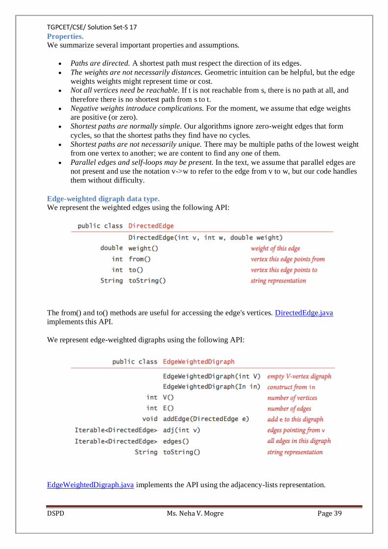
TGPCET/CSE/ Solution Set-S 17
DSPD Ms. Neha V. Mogre Page 39
Properties.
We summarize several important properties and assumptions.
Paths are directed. A shortest path must respect the direction of its edges.
The weights are not necessarily distances. Geometric intuition can be helpful, but the edge
weights weights might represent time or cost.
Not all vertices need be reachable. If t is not reachable from s, there is no path at all, and
therefore there is no shortest path from s to t.
Negative weights introduce complications. For the moment, we assume that edge weights
are positive (or zero).
Shortest paths are normally simple. Our algorithms ignore zero-weight edges that form
cycles, so that the shortest paths they find have no cycles.
Shortest paths are not necessarily unique. There may be multiple paths of the lowest weight
from one vertex to another; we are content to find any one of them.
Parallel edges and self-loops may be present. In the text, we assume that parallel edges are
not present and use the notation v->w to refer to the edge from v to w, but our code handles
them without difficulty.
Edge-weighted digraph data type.
We represent the weighted edges using the following API:
The from() and to() methods are useful for accessing the edge's vertices. DirectedEdge.java
implements this API.
We represent edge-weighted digraphs using the following API:
EdgeWeightedDigraph.java implements the API using the adjacency-lists representation.
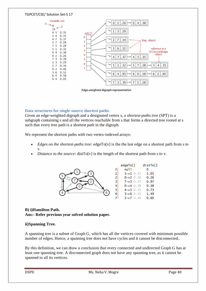
TGPCET/CSE/ Solution Set-S 17
DSPD Ms. Neha V. Mogre Page 40
Data structures for single-source shortest paths.
Given an edge-weighted digraph and a designated vertex s, a shortest-paths tree (SPT) is a
subgraph containing s and all the vertices reachable from s that forms a directed tree rooted at s
such that every tree path is a shortest path in the digraph.
We represent the shortest paths with two vertex-indexed arrays:
Edges on the shortest-paths tree: edgeTo[v] is the the last edge on a shortest path from s to
v.
Distance to the source: distTo[v] is the length of the shortest path from s to v.
B) i)Hamilton Path.
Ans:- Refer previous year solved solution paper.
ii)Spanning Tree.
A spanning tree is a subset of Graph G, which has all the vertices covered with minimum possible
number of edges. Hence, a spanning tree does not have cycles and it cannot be disconnected..
By this definition, we can draw a conclusion that every connected and undirected Graph G has at
least one spanning tree. A disconnected graph does not have any spanning tree, as it cannot be
spanned to all its vertices.

TGPCET/CSE/ Solution Set-S 17
DSPD Ms. Neha V. Mogre Page 41
We found three spanning trees off one complete graph. A complete undirected graph can have
maximum nn-2 number of spanning trees, where n is the number of nodes. In the above addressed
example, 33−2 = 3 spanning trees are possible.
General Properties of Spanning Tree
We now understand that one graph can have more than one spanning tree. Following are a few
properties of the spanning tree connected to graph G −
A connected graph G can have more than one spanning tree.
All possible spanning trees of graph G, have the same number of edges and vertices.
The spanning tree does not have any cycle (loops).
Removing one edge from the spanning tree will make the graph disconnected, i.e. the
spanning tree is minimally connected.
Adding one edge to the spanning tree will create a circuit or loop, i.e. the spanning tree is
maximally acyclic.
Mathematical Properties of Spanning Tree
Spanning tree has n-1 edges, where n is the number of nodes (vertices).
From a complete graph, by removing maximum e - n + 1 edges, we can construct a
spanning tree.
A complete graph can have maximum nn-2 number of spanning trees.
Thus, we can conclude that spanning trees are a subset of connected Graph G and disconnected
graphs do not have spanning tree.
Application of Spanning Tree
Spanning tree is basically used to find a minimum path to connect all nodes in a graph. Common
application of spanning trees are −
Civil Network Planning
Computer Network Routing Protocol
Cluster Analysis
Let us understand this through a small example. Consider, city network as a huge graph and now
plans to deploy telephone lines in such a way that in minimum lines we can connect to all city
nodes. This is where the spanning tree comes into picture.
TGPCET/CSE/ Solution Set-S 17
DSPD Ms. Neha V. Mogre Page 42
Minimum Spanning Tree (MST)
In a weighted graph, a minimum spanning tree is a spanning tree that has minimum weight than all
other spanning trees of the same graph. In real-world situations, this weight can be measured as
distance, congestion, traffic load or any arbitrary value denoted to the edges.
Minimum Spanning-Tree Algorithm
We shall learn about two most important spanning tree algorithms here −
Kruskal's Algorithm
Prim's Algorithm
Both are greedy algorithms.
11A)What is collision in hashing ? How can it be avoided ? What are the different collision
handling mechanisms ? Explain each with suitable example
Ans:- Refer previous year solved solution paper.
12) What is symbol table ? What are different data structures used for symbol table ? Discuss.
In computer science, a symbol table is a data structure used by a language translator such as a
compiler or interpreter, where each identifier in a program's source code is associated with
information relating to its declaration or appearance in the source.
Implementation
A common implementation technique is to use a hash table. A compiler may use one large symbol
table for all symbols or use separated, hierarchical symbol tables for different scopes. There are also
trees, linear lists and self-organizing lists which can be used to implement a symbol table. It also
simplifies the classification of literals in tabular format. The symbol table is accessed by most
phases of a compiler, beginning with the lexical analysis to optimization.
Uses
An object file will contain a symbol table of the identifiers it contains that are externally visible.
During the linking of different object files, a linker will use these symbol tables to resolve any
unresolved references.
A symbol table may only exist during the translation process, or it may be embedded in the output
of that process for later exploitation, for example, during an interactive debugging session, or as a
resource for formatting a diagnostic report during or after execution of a program.
While reverse engineering an executable, many tools refer to the symbol table to check what
addresses have been assigned to global variables and known functions. If the symbol table has been
stripped or cleaned out before being converted into an executable, tools will find it harder to
determine addresses or understand anything about the program.
At that time of accessing variables and allocating memory dynamically, a compiler should perform
many works and as such the extended stack model requires the symbol table.
Example
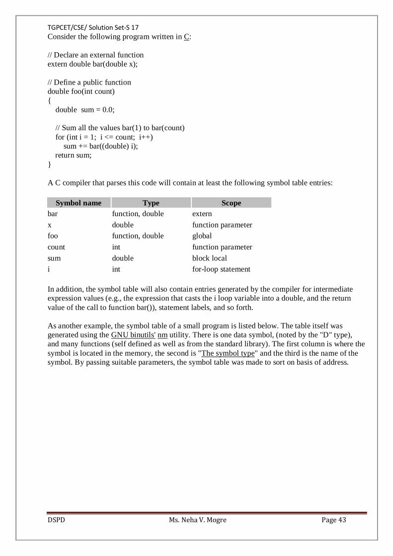
TGPCET/CSE/ Solution Set-S 17
DSPD Ms. Neha V. Mogre Page 43
Consider the following program written in C:
// Declare an external function
extern double bar(double x);
// Define a public function
double foo(int count)
{
double sum = 0.0;
// Sum all the values bar(1) to bar(count)
for (int i = 1; i <= count; i++)
sum += bar((double) i);
return sum;
}
A C compiler that parses this code will contain at least the following symbol table entries:
Symbol name Type Scope
bar function, double extern
x double function parameter
foo function, double global
count int function parameter
sum double block local
i int for-loop statement
In addition, the symbol table will also contain entries generated by the compiler for intermediate
expression values (e.g., the expression that casts the i loop variable into a double, and the return
value of the call to function bar()), statement labels, and so forth.
As another example, the symbol table of a small program is listed below. The table itself was
generated using the GNU binutils' nm utility. There is one data symbol, (noted by the "D" type),
and many functions (self defined as well as from the standard library). The first column is where the
symbol is located in the memory, the second is "The symbol type" and the third is the name of the
symbol. By passing suitable parameters, the symbol table was made to sort on basis of address.

TGPCET/CSE/ Solution Set-W 17
DSPD Ms. Neha V. Mogre Page 1
Tulsiramji Gaikwad-Patil College of Engineering and Technology
Department of Computer Science and Engineering
Semester : B.E. Fourth Semester
Subject : DSPD
Solution Set: Winter – 2017
1a) Explain the various sorting techniques. Give its time complexities.
Bubble Sort [Best: O(n), Worst:O(N^2)]
Starting on the left, compare adjacent items and keep “bubbling” the larger one to the right (it’s in
its final place). Bubble sort the remaining N -1 items.
Though “simple” I found bubble sort nontrivial. In general, sorts where you iterate
backwards (decreasing some index) were counter-intuitive for me. With bubble-sort, either
you bubble items “forward” (left-to-right) and move the endpoint backwards (decreasing),
or bubble items “backward” (right-to-left) and increase the left endpoint. Either way, some
index is decreasing.
You also need to keep track of the next-to-last endpoint, so you don’t swap with a non-
existent item.
Selection Sort [Best/Worst: O(N^2)]
Scan all items and find the smallest. Swap it into position as the first item. Repeat the selection sort
on the remaining N-1 items.
I found this the most intuitive and easiest to implement — you always iterate forward (i
from 0 to N-1), and swap with the smallest element (always i).
Insertion Sort [Best: O(N), Worst:O(N^2)]
Start with a sorted list of 1 element on the left, and N-1 unsorted items on the right. Take the first
unsorted item (element #2) and insert it into the sorted list, moving elements as necessary. We now
have a sorted list of size 2, and N -2 unsorted elements. Repeat for all elements.
Like bubble sort, I found this counter-intuitive because you step “backwards”
This is a little like bubble sort for moving items, except when you encounter an item smaller
than you, you stop. If the data is reverse-sorted, each item must travel to the head of the list,
and this becomes bubble-sort.
There are various ways to move the item leftwards — you can do a swap on each iteration,
or copy each item over its neighbor
Radix sort [Best/Avg/Worst: O(N)]
Get a series of numbers, and sort them one digit at a time (moving all the 1000’s ahead of the
2000’s, etc.). Repeat the sorting on each set of digits.
Radix sort uses counting sort for efficient O(N) sorting of the digits (k = 0…9)
Actually, radix sort goes from least significant digit (1’s digit) to most significant, for
reasons I’ll explain later (see CLRS book)
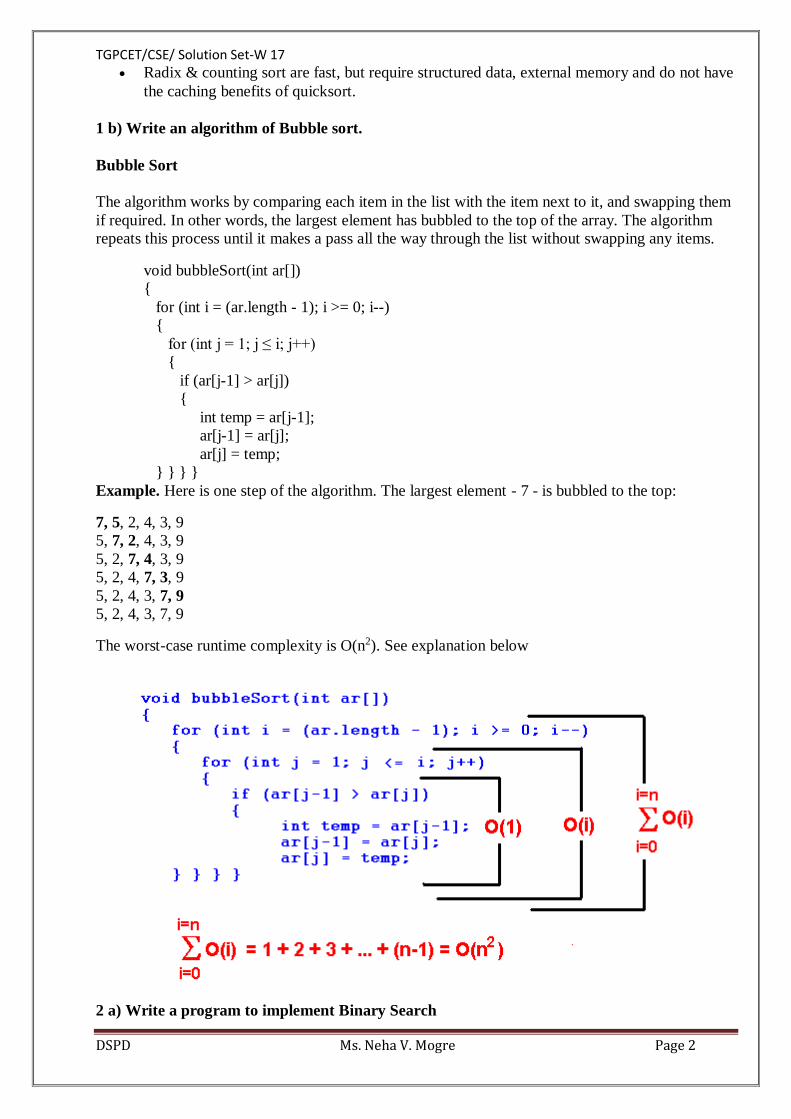
TGPCET/CSE/ Solution Set-W 17
DSPD Ms. Neha V. Mogre Page 2
Radix & counting sort are fast, but require structured data, external memory and do not have
the caching benefits of quicksort.
1 b) Write an algorithm of Bubble sort.
Bubble Sort
The algorithm works by comparing each item in the list with the item next to it, and swapping them
if required. In other words, the largest element has bubbled to the top of the array. The algorithm
repeats this process until it makes a pass all the way through the list without swapping any items.
void bubbleSort(int ar[])
{
for (int i = (ar.length - 1); i >= 0; i--)
{
for (int j = 1; j ≤ i; j++)
{
if (ar[j-1] > ar[j])
{
int temp = ar[j-1];
ar[j-1] = ar[j];
ar[j] = temp;
} } } }
Example. Here is one step of the algorithm. The largest element - 7 - is bubbled to the top:
7, 5, 2, 4, 3, 9
5, 7, 2, 4, 3, 9
5, 2, 7, 4, 3, 9
5, 2, 4, 7, 3, 9
5, 2, 4, 3, 7, 9
5, 2, 4, 3, 7, 9
The worst-case runtime complexity is O(n2). See explanation below
2 a) Write a program to implement Binary Search
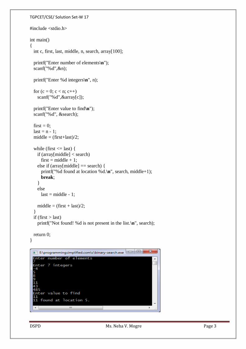
TGPCET/CSE/ Solution Set-W 17
DSPD Ms. Neha V. Mogre Page 3
#include <stdio.h>
int main()
{
int c, first, last, middle, n, search, array[100];
printf("Enter number of elements\n");
scanf("%d",&n);
printf("Enter %d integers\n", n);
for (c = 0; c < n; c++)
scanf("%d",&array[c]);
printf("Enter value to find\n");
scanf("%d", &search);
first = 0;
last = n - 1;
middle = (first+last)/2;
while (first <= last) {
if (array[middle] < search)
first = middle + 1;
else if (array[middle] == search) {
printf("%d found at location %d.\n", search, middle+1);
break;
}
else
last = middle - 1;
middle = (first + last)/2;
}
if (first > last)
printf("Not found! %d is not present in the list.\n", search);
return 0;
}
TGPCET/CSE/ Solution Set-W 17
DSPD Ms. Neha V. Mogre Page 4
2b) Explain the following terms :––
i)Sparse Matrix.
What is Sparse Matrix?
In computer programming, a matrix can be defined with a 2-dimensional array. Any array with 'm'
columns and 'n' rows represents a mXn matrix. There may be a situation in which a matrix contains
more number of ZERO values than NON-ZERO values. Such matrix is known as sparse matrix.
Sparse matrix is a matrix which contains very few non-zero elements.
When a sparse matrix is represented with 2-dimensional array, we waste lot of space to represent
that matrix. For example, consider a matrix of size 100 X 100 containing only 10 non-zero
elements. In this matrix, only 10 spaces are filled with non-zero values and remaining spaces of
matrix are filled with zero. That means, totally we allocate 100 X 100 X 2 = 20000 bytes of space to
store this integer matrix. And to access these 10 non-zero elements we have to make scanning for
10000 times.
Sparse Matrix Representations
A sparse matrix can be represented by using TWO representations, those are as follows...
1. Triplet Representation
2. Linked Representation
Triplet Representation
In this representation, we consider only non-zero values along with their row and column index
values. In this representation, the 0th row stores total rows, total columns and total non-zero values
in the matrix.
For example, consider a matrix of size 5 X 6 containing 6 number of non-zero values. This matrix
can be represented as shown in the image...
In above example matrix, there are only 6 non-zero elements ( those are 9, 8, 4, 2, 5 & 2) and
matrix size is 5 X 6. We represent this matrix as shown in the above image. Here the first row in the
right side table is filled with values 5, 6 & 6 which indicates that it is a sparse matrix with 5 rows, 6
columns & 6 non-zero values. Second row is filled with 0, 4, & 9 which indicates the value in the
matrix at 0th row, 4th column is 9. In the same way the remaining non-zero values also follows the
similar pattern.
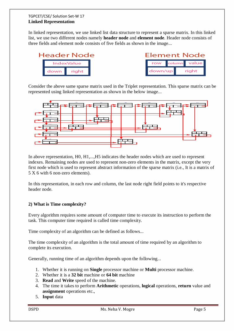
TGPCET/CSE/ Solution Set-W 17
DSPD Ms. Neha V. Mogre Page 5
Linked Representation
In linked representation, we use linked list data structure to represent a sparse matrix. In this linked
list, we use two different nodes namely header node and element node. Header node consists of
three fields and element node consists of five fields as shown in the image...
Consider the above same sparse matrix used in the Triplet representation. This sparse matrix can be
represented using linked representation as shown in the below image...
In above representation, H0, H1,...,H5 indicates the header nodes which are used to represent
indexes. Remaining nodes are used to represent non-zero elements in the matrix, except the very
first node which is used to represent abstract information of the sparse matrix (i.e., It is a matrix of
5 X 6 with 6 non-zero elements).
In this representation, in each row and column, the last node right field points to it's respective
header node.
2) What is Time complexity?
Every algorithm requires some amount of computer time to execute its instruction to perform the
task. This computer time required is called time complexity.
Time complexity of an algorithm can be defined as follows...
The time complexity of an algorithm is the total amount of time required by an algorithm to
complete its execution.
Generally, running time of an algorithm depends upon the following...
1. Whether it is running on Single processor machine or Multi processor machine.
2. Whether it is a 32 bit machine or 64 bit machine
3. Read and Write speed of the machine.
4. The time it takes to perform Arithmetic operations, logical operations, return value and
assignment operations etc.,
5. Input data
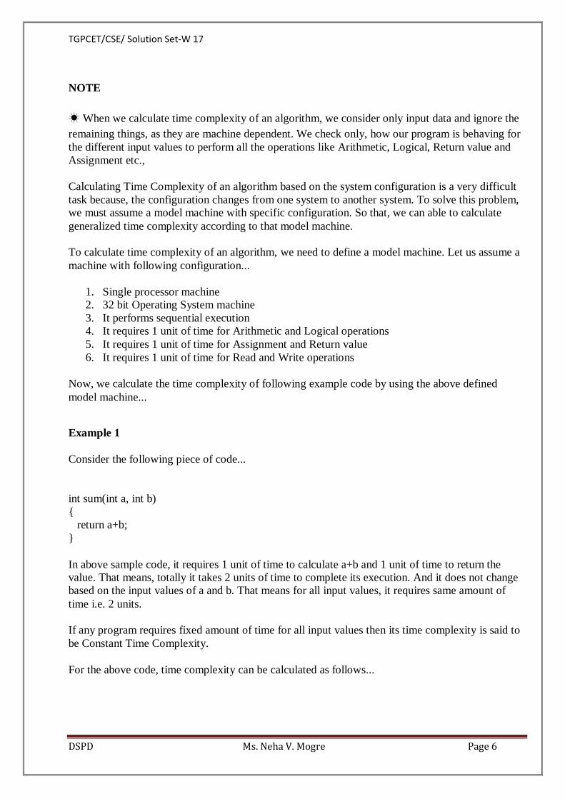
TGPCET/CSE/ Solution Set-W 17
DSPD Ms. Neha V. Mogre Page 6
NOTE
☀ When we calculate time complexity of an algorithm, we consider only input data and ignore the
remaining things, as they are machine dependent. We check only, how our program is behaving for
the different input values to perform all the operations like Arithmetic, Logical, Return value and
Assignment etc.,
Calculating Time Complexity of an algorithm based on the system configuration is a very difficult
task because, the configuration changes from one system to another system. To solve this problem,
we must assume a model machine with specific configuration. So that, we can able to calculate
generalized time complexity according to that model machine.
To calculate time complexity of an algorithm, we need to define a model machine. Let us assume a
machine with following configuration...
1. Single processor machine
2. 32 bit Operating System machine
3. It performs sequential execution
4. It requires 1 unit of time for Arithmetic and Logical operations
5. It requires 1 unit of time for Assignment and Return value
6. It requires 1 unit of time for Read and Write operations
Now, we calculate the time complexity of following example code by using the above defined
model machine...
Example 1
Consider the following piece of code...
int sum(int a, int b)
{
return a+b;
}
In above sample code, it requires 1 unit of time to calculate a+b and 1 unit of time to return the
value. That means, totally it takes 2 units of time to complete its execution. And it does not change
based on the input values of a and b. That means for all input values, it requires same amount of
time i.e. 2 units.
If any program requires fixed amount of time for all input values then its time complexity is said to
be Constant Time Complexity.
For the above code, time complexity can be calculated as follows...
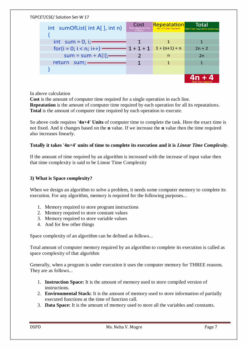
TGPCET/CSE/ Solution Set-W 17
DSPD Ms. Neha V. Mogre Page 7
In above calculation
Cost is the amount of computer time required for a single operation in each line.
Repeatation is the amount of computer time required by each operation for all its repeatations.
Total is the amount of computer time required by each operation to execute.
So above code requires '4n+4' Units of computer time to complete the task. Here the exact time is
not fixed. And it changes based on the n value. If we increase the n value then the time required
also increases linearly.
Totally it takes '4n+4' units of time to complete its execution and it is Linear Time Complexity.
If the amount of time required by an algorithm is increased with the increase of input value then
that time complexity is said to be Linear Time Complexity
3) What is Space complexity?
When we design an algorithm to solve a problem, it needs some computer memory to complete its
execution. For any algorithm, memory is required for the following purposes...
1. Memory required to store program instructions
2. Memory required to store constant values
3. Memory required to store variable values
4. And for few other things
Space complexity of an algorithm can be defined as follows...
Total amount of computer memory required by an algorithm to complete its execution is called as
space complexity of that algorithm
Generally, when a program is under execution it uses the computer memory for THREE reasons.
They are as follows...
1. Instruction Space: It is the amount of memory used to store compiled version of
instructions.
2. Environmental Stack: It is the amount of memory used to store information of partially
executed functions at the time of function call.
3. Data Space: It is the amount of memory used to store all the variables and constants.
TGPCET/CSE/ Solution Set-W 17
DSPD Ms. Neha V. Mogre Page 8
NOTE
☀ When we want to perform analysis of an algorithm based on its Space complexity, we consider
only Data Space and ignore Instruction Space as well as Environmental Stack.
That means we calculate only the memory required to store Variables, Constants, Structures, etc.,
To calculate the space complexity, we must know the memory required to store different datatype
values (according to the compiler). For example, the C Programming Language compiler requires
the following...
1. 2 bytes to store Integer value,
2. 4 bytes to store Floating Point value,
3. 1 byte to store Character value,
4. 6 (OR) 8 bytes to store double value
Example 1
Consider the following piece of code...
int square(int a)
{
return a*a;
}
In above piece of code, it requires 2 bytes of memory to store variable 'a' and another 2 bytes of
memory is used for return value.
That means, totally it requires 4 bytes of memory to complete its execution. And this 4 bytes
of memory is fixed for any input value of 'a'. This space complexity is said to be Constant
Space Complexity.
If any algorithm requires a fixed amount of space for all input values then that space complexity is
said to be Constant Space Complexity
Example 2
Consider the following piece of code...
int sum(int A[], int n)
{
int sum = 0, i;
for(i = 0; i < n; i++)
sum = sum + A[i];
return sum;
}
In above piece of code it requires
TGPCET/CSE/ Solution Set-W 17
DSPD Ms. Neha V. Mogre Page 9
'n*2' bytes of memory to store array variable 'a[]'
2 bytes of memory for integer parameter 'n'
4 bytes of memory for local integer variables 'sum' and 'i' (2 bytes each)
2 bytes of memory for return value.
That means, totally it requires '2n+8' bytes of memory to complete its execution. Here, the
amount of memory depends on the input value of 'n'. This space complexity is said to be
Linear Space Complexity.
If the amount of space required by an algorithm is increased with the increase of input value, then
that space complexity is said to be Linear Space Complexity
3a) Write a Menu Driven Program for various operations of singly linked list.
#include<stdio.h>
#include<conio.h>
#include<process.h>
struct node
{
int data;
struct node *next;
}*start=NULL,*q,*t;
int main()
{
int ch;
void insert_beg();
void insert_end();
int insert_pos();
void display();
void delete_beg();
void delete_end();
int delete_pos();
while(1)
{
printf("\n\n---- Singly Linked List(SLL) Menu ----");
printf("\n1.Insert\n2.Display\n3.Delete\n4.Exit\n\n");
printf("Enter your choice(1-4):");
scanf("%d",&ch);
switch(ch)
{
case 1:
printf("\n---- Insert Menu ----");
printf("\n1.Insert at beginning\n2.Insert at end\n3.Insert at specified position\n4.Exit");
printf("\n\nEnter your choice(1-4):");
scanf("%d",&ch);
switch(ch)
{
case 1: insert_beg();
TGPCET/CSE/ Solution Set-W 17
DSPD Ms. Neha V. Mogre Page 10
break;
case 2: insert_end();
break;
case 3: insert_pos();
break;
case 4: exit(0);
default: printf("Wrong Choice!!");
}
break;
case 2: display();
break;
case 3: printf("\n---- Delete Menu ----");
printf("\n1.Delete from beginning\n2.Delete from end\n3.Delete from specified
position\n4.Exit");
printf("\n\nEnter your choice(1-4):");
scanf("%d",&ch);
switch(ch)
{
case 1: delete_beg();
break;
case 2: delete_end();
break;
case 3: delete_pos();
break;
case 4: exit(0);
default: printf("Wrong Choice!!");
}
break;
case 4: exit(0);
default: printf("Wrong Choice!!");
}
}
return 0;
}
void insert_beg()
{
int num;
t=(struct node*)malloc(sizeof(struct node));
printf("Enter data:");
scanf("%d",&num);
t->data=num;
if(start==NULL) //If list is empty
{
t->next=NULL;
start=t;
}
else

TGPCET/CSE/ Solution Set-W 17
DSPD Ms. Neha V. Mogre Page 11
{
t->next=start;
start=t;
}
}
void insert_end()
{
int num;
t=(struct node*)malloc(sizeof(struct node));
printf("Enter data:");
scanf("%d",&num);
t->data=num;
t->next=NULL;
if(start==NULL) //If list is empty
{
start=t;
}
else
{
q=start;
while(q->next!=NULL)
q=q->next;
q->next=t;
}
}
int insert_pos()
{
int pos,i,num;
if(start==NULL)
{
printf("List is empty!!");
return 0;
}
t=(struct node*)malloc(sizeof(struct node));
printf("Enter data:");
scanf("%d",&num);
printf("Enter position to insert:");
scanf("%d",&pos);
t->data=num;
q=start;
for(i=1;i<pos-1;pos++)
{
if(q->next==NULL)
{
printf("There are less elements!!");
return 0;
}
TGPCET/CSE/ Solution Set-W 17
DSPD Ms. Neha V. Mogre Page 12
q=q->next;
}
t->next=q->next;
q->next=t;
return 0;
}
void display()
{
if(start==NULL)
{
printf("List is empty!!");
}
else
{
q=start;
printf("The linked list is:\n");
while(q!=NULL)
{
printf("%d->",q->data);
q=q->next;
}
}
}
void delete_beg()
{
if(start==NULL)
{
printf("The list is empty!!");
}
else
{
q=start;
start=start->next;
printf("Deleted element is %d",q->data);
free(q);
}
}
void delete_end()
{
if(start==NULL)
{
printf("The list is empty!!");
}
else
{
q=start;
while(q->next->next!=NULL)
TGPCET/CSE/ Solution Set-W 17
DSPD Ms. Neha V. Mogre Page 13
q=q->next;
t=q->next;
q->next=NULL;
printf("Deleted element is %d",t->data);
free(t);
}
}
int delete_pos()
{
int pos,i;
if(start==NULL)
{
printf("List is empty!!");
return 0;
}
printf("Enter position to delete:");
scanf("%d",&pos);
for(i=1;i<pos-1;pos++)
{
if(q->next==NULL)
{
printf("There are less elements!!");
return 0;
}
q=q->next;
}
t=q->next;
q->next=t->next;
printf("Deleted element is %d",t->data);
free(t);
return 0;
}
Output —- Singly Linked List(SLL) Menu —-
1.Insert
2.Display
3.Delete
4.ExitEnter your choice(1-4):1—- Insert Menu —-
1.Insert at beginning
2.Insert at end
3.Insert at specified position
4.Exit

TGPCET/CSE/ Solution Set-W 17
DSPD Ms. Neha V. Mogre Page 14
Enter your choice(1-4):1
Enter data:4
—- Singly Linked List(SLL) Menu —-
1.Insert
2.Display
3.Delete
4.Exit
Enter your choice(1-4):2
The linked list is:
4->
—- Singly Linked List(SLL) Menu —-
1.Insert
2.Display
3.Delete
4.Exit
Enter your choice(1-4):4
3 b) Give suitable representation for polynomials and write an algorithm to add two
polynomials.
Program to add two polynomials
Given two polynomials represented by two arrays, write a function that adds given two
polynomials.
Example:
Input: A[] = {5, 0, 10, 6}
B[] = {1, 2, 4}
Output: sum[] = {5, 10, 30, 26, 52, 24}
The first input array represents "5 + 0x^1 + 10x^2 + 6x^3"
The second array represents "1 + 2x^1 + 4x^2"
And Output is "6 + 2x^1 + 14x^2 + 6x^3"
Addition is simpler than multiplication of polynomials. We initialize result as one of the two
polynomials, then we traverse the other polynomial and add all terms to the result.
add(A[0..m-1], B[0..n01])
1) Create a sum array sum[] of size equal to maximum of 'm' and 'n'
2) Copy A[] to sum[].
3) Travers array B[] and do following for every element B[i]
sum[i] = sum[i] + B[i]
4) Return sum[].
The following is C++ implementation of above algorithm.

TGPCET/CSE/ Solution Set-W 17
DSPD Ms. Neha V. Mogre Page 15
// Simple C++ program to add two polynomials
#include <iostream>
using namespace std;
// A utility function to return maximum of two integers
int max(int m, int n) { return (m > n)? m: n; }
// A[] represents coefficients of first polynomial
// B[] represents coefficients of second polynomial
// m and n are sizes of A[] and B[] respectively
int *add(int A[], int B[], int m, int n)
{
int size = max(m, n);
int *sum = new int[size];
// Initialize the porduct polynomial
for (int i = 0; i<m; i++)
sum[i] = A[i];
// Take ever term of first polynomial
for (int i=0; i<n; i++)
sum[i] += B[i];
return sum;
}
// A utility function to print a polynomial
void printPoly(int poly[], int n)
{
for (int i=0; i<n; i++)
TGPCET/CSE/ Solution Set-W 17
DSPD Ms. Neha V. Mogre Page 16
{
cout << poly[i];
if (i != 0)
cout << "x^" << i ;
if (i != n-1)
cout << " + ";
}
}
// Driver program to test above functions
int main()
{
// The following array represents polynomial 5 + 10x^2 + 6x^3
int A[] = {5, 0, 10, 6};
// The following array represents polynomial 1 + 2x + 4x^2
int B[] = {1, 2, 4};
int m = sizeof(A)/sizeof(A[0]);
int n = sizeof(B)/sizeof(B[0]);
cout << "First polynomial is \n";
printPoly(A, m);
cout << "\nSecond polynomial is \n";
printPoly(B, n);
int *sum = add(A, B, m, n);
int size = max(m, n);
cout << "\nsumuct polynomial is \n";
printPoly(sum, size);
TGPCET/CSE/ Solution Set-W 17
DSPD Ms. Neha V. Mogre Page 17
return 0;
}
Output:
First polynomial is
5 + 0x^1 + 10x^2 + 6x^3
Second polynomial is
1 + 2x^1 + 4x^2
Sum polynomial is
6 + 2x^1 + 14x^2 + 6x^3
Time complexity of the above algorithm and program is O(m+n) where m and n are orders of two
given polynomials.
4) Write a function to :––
(i) Insert a node at end in doubly linked list
Insertion At Last in doubly linked list
Algorithm
1. InsertAtEndDll(info,prev,next,start,end)
2. 1.create a new node and address in assigned to ptr.
3. 2.check[overflow] if(ptr=NULL)
4. write:overflow and exit
5. 3.set Info[ptr]=item;
6. 4.if(start=NULL)
7. set prev[ptr] = next[ptr] = NULL
8. set start = end = ptr
9. else
10. set prev[ptr] = end
11. next[end] = ptr
12. set ptr[next] = NULL
13. set end = ptr
14. [end if]
15. 5.Exit.
b)Delete a node from a specific position from doubly linked list.
Algorithm to delete node from any position of a doubly linked list
Algorithm to delete node from any position
%% Input : head {Pointer to the first node of the list}

TGPCET/CSE/ Solution Set-W 17
DSPD Ms. Neha V. Mogre Page 18
last {Pointer to the last node of the list}
N {Position to be deleted from list}
Begin:
current ← head;
For i ← 1 to N and current != NULL do
current ← current.next;
End for
If (N == 1) then
deleteFromBeginning()
End if Else if (current == last) then
deleteFromEnd()
End if
Else if (current != NULL) then
current.prev.next ← current.next
If (current.next != NULL) then
current.next.prev ← current.prev;
End if unalloc (current)
write ('Node deleted successfully from ', N, ' position')
End if
Else then
write ('Invalid position')
End if
End
4b) What is static memory allocation and dynamic memory allocation ? What are the
functions used for dynamic memory allocation in ''C'' ? Give examples.
static memory allocation and dynamic memory allocation:-
Static Memory Allocation: Memory is allocated for the declared variable by the compiler. The
address can be obtained by using ‘address of’ operator and can be assigned to a pointer. The
memory is allocated during compile time. Since most of the declared variables have static memory,
this kind of assigning the address of a variable to a pointer is known as static memory allocation.
Dynamic Memory Allocation: Allocation of memory at the time of execution (run time) is known
as dynamic memory allocation. The functions calloc() and malloc() support allocating of dynamic
memory. Dynamic allocation of memory space is done by using these functions when value is
returned by functions and assigned to pointer variables.
In C, the exact size of array is unknown until compile time, i.e., the time when a compiler compiles
your code into a computer understandable language. So, sometimes the size of the array can be
insufficient or more than required.
Dynamic memory allocation allows your program to obtain more memory space while running, or
to release it if it's not required.
In simple terms, Dynamic memory allocation allows you to manually handle memory space for
your program.
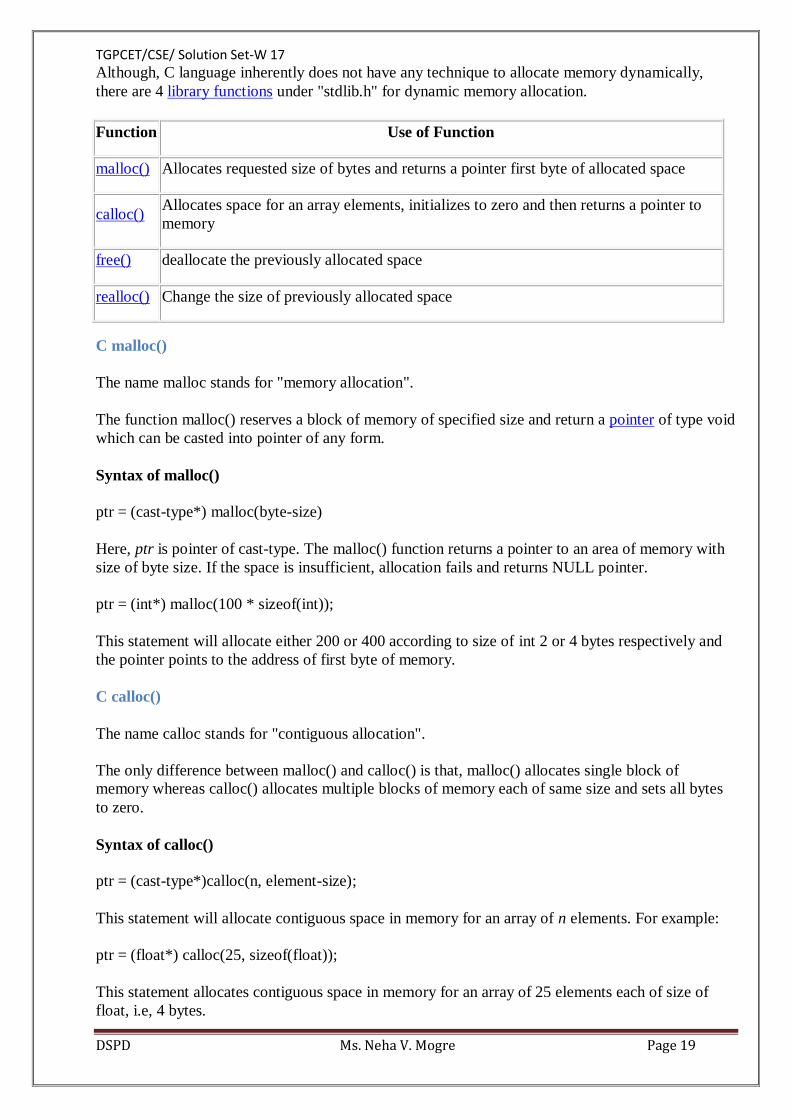
TGPCET/CSE/ Solution Set-W 17
DSPD Ms. Neha V. Mogre Page 19
Although, C language inherently does not have any technique to allocate memory dynamically,
there are 4 library functions under "stdlib.h" for dynamic memory allocation.
Function Use of Function
malloc() Allocates requested size of bytes and returns a pointer first byte of allocated space
calloc()
Allocates space for an array elements, initializes to zero and then returns a pointer to
memory
free() deallocate the previously allocated space
realloc() Change the size of previously allocated space
C malloc()
The name malloc stands for "memory allocation".
The function malloc() reserves a block of memory of specified size and return a pointer of type void
which can be casted into pointer of any form.
Syntax of malloc()
ptr = (cast-type*) malloc(byte-size)
Here, ptr is pointer of cast-type. The malloc() function returns a pointer to an area of memory with
size of byte size. If the space is insufficient, allocation fails and returns NULL pointer.
ptr = (int*) malloc(100 * sizeof(int));
This statement will allocate either 200 or 400 according to size of int 2 or 4 bytes respectively and
the pointer points to the address of first byte of memory.
C calloc()
The name calloc stands for "contiguous allocation".
The only difference between malloc() and calloc() is that, malloc() allocates single block of
memory whereas calloc() allocates multiple blocks of memory each of same size and sets all bytes
to zero.
Syntax of calloc()
ptr = (cast-type*)calloc(n, element-size);
This statement will allocate contiguous space in memory for an array of n elements. For example:
ptr = (float*) calloc(25, sizeof(float));
This statement allocates contiguous space in memory for an array of 25 elements each of size of
float, i.e, 4 bytes.
TGPCET/CSE/ Solution Set-W 17
DSPD Ms. Neha V. Mogre Page 20
C free()
Dynamically allocated memory created with either calloc() or malloc() doesn't get freed on its own.
You must explicitly use free() to release the space.
syntax of free()
free(ptr);
This statement frees the space allocated in the memory pointed by ptr.
5a) Write an algorithm which convert infix expression into postfix from using stack and give
steps of each.
nfix to Postfix Conversion
Procedure for Postfix Conversion
1. Scan the Infix string from left to right.
2. Initialize an empty stack.
3. If the scanned character is an operand, add it to the Postfix string.
4. If the scanned character is an operator and if the stack is empty push the character to stack.
5. If the scanned character is an Operator and the stack is not empty, compare the precedence of
the character with the element on top of the stack.
6.
If top Stack has higher precedence over the scanned character pop the stack else push the
scanned character to stack. Repeat this step until the stack is not empty and top Stack has
precedence over the character.
7. Repeat 4 and 5 steps till all the characters are scanned.
8. After all characters are scanned, we have to add any character that the stack may have to the
Postfix string.
9. If stack is not empty add top Stack to Postfix string and Pop the stack.
10. Repeat this step as long as stack is not empty.
Algorithm for Postfix Conversion
1. S:stack
2. while(more tokens)
3. x<=next token
4. if(x == operand)
5. print x
6. else
7. while(precedence(x)<=precedence(top(s)))

TGPCET/CSE/ Solution Set-W 17
DSPD Ms. Neha V. Mogre Page 21
8. print(pop(s))
9. push(s,x)
10. while(! empty (s))
11. print(pop(s))
Conversion To Postfix
EXAMPLE:
A+(B*C-(D/E-F)*G)*H
Stack Input Output
Empty A+(B*C-(D/E-F)*G)*H -
Empty +(B*C-(D/E-F)*G)*H A
+ (B*C-(D/E-F)*G)*H A
+( B*C-(D/E-F)*G)*H A
+( *C-(D/E-F)*G)*H AB
+(* C-(D/E-F)*G)*H AB
+(* -(D/E-F)*G)*H ABC
+(- (D/E-F)*G)*H ABC*
+(-( D/E-F)*G)*H ABC*
+(-( /E-F)*G)*H ABC*D
+(-(/ E-F)*G)*H ABC*D
+(-(/ -F)*G)*H ABC*DE
+(-(- F)*G)*H ABC*DE/
+(-(- F)*G)*H ABC*DE/
+(-(- )*G)*H ABC*DE/F
+(- *G)*H ABC*DE/F-
+(-* G)*H ABC*DE/F-
+(-* )*H ABC*DE/F-G
+ *H ABC*DE/F-G*-
+* H ABC*DE/F-G*-
+* End ABC*DE/F-G*-H
TGPCET/CSE/ Solution Set-W 17
DSPD Ms. Neha V. Mogre Page 22
Empty End ABC*DE/F-G*-H*+
Infix to postfix implementation in c
1. #include <stdio.h>
2. #include <conio.h>
3. #include <ctype.h>
4. #define SIZE 50
5. char s[SIZE];
6. int top=-1;
7. push(char elem)
8. {
9. s[++top]=elem;
10. }
11.
12. char pop()
13. {
14. return(s[top--]);
15. }
16.
17. int pr(char elem)
18. {
19. switch(elem)
20. {
21. case '#': return 0;
22. case '(': return 1;
23. case '+':
24. case '-': return 2;
25. case '*':
26. case '/': return 3;
27. }
28. }
29.
30. void main()
31. {
32. char infx[50],pofx[50],ch,elem;
33. int i=0,k=0;
34. clrscr();
35. printf("\n\nRead the Infix Expression ? ");
36. scanf("%s",infx);
37. push('#');
38. while( (ch=infx[i++]) != '\0')
39. {
40. if( ch == '(') push(ch);
41. else
42. if(isalnum(ch)) pofx[k++]=ch;
43. else
44. if( ch == ')')
45. {
46. while( s[top] != '(')
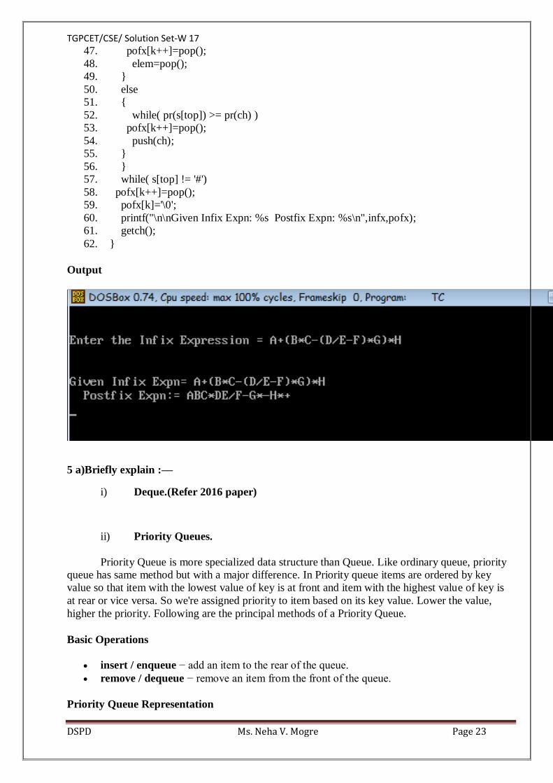
TGPCET/CSE/ Solution Set-W 17
DSPD Ms. Neha V. Mogre Page 23
47. pofx[k++]=pop();
48. elem=pop();
49. }
50. else
51. {
52. while( pr(s[top]) >= pr(ch) )
53. pofx[k++]=pop();
54. push(ch);
55. }
56. }
57. while( s[top] != '#')
58. pofx[k++]=pop();
59. pofx[k]='\0';
60. printf("\n\nGiven Infix Expn: %s Postfix Expn: %s\n",infx,pofx);
61. getch();
62. }
Output
5 a)Briefly explain :––
i) Deque.(Refer 2016 paper)
ii) Priority Queues.
Priority Queue is more specialized data structure than Queue. Like ordinary queue, priority
queue has same method but with a major difference. In Priority queue items are ordered by key
value so that item with the lowest value of key is at front and item with the highest value of key is
at rear or vice versa. So we're assigned priority to item based on its key value. Lower the value,
higher the priority. Following are the principal methods of a Priority Queue.
Basic Operations
insert / enqueue − add an item to the rear of the queue.
remove / dequeue − remove an item from the front of the queue.
Priority Queue Representation
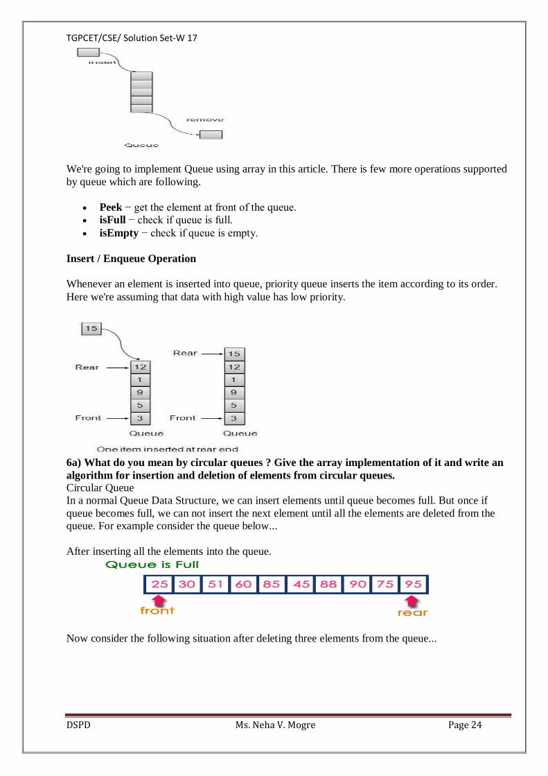
TGPCET/CSE/ Solution Set-W 17
DSPD Ms. Neha V. Mogre Page 24
We're going to implement Queue using array in this article. There is few more operations supported
by queue which are following.
Peek − get the element at front of the queue.
isFull − check if queue is full.
isEmpty − check if queue is empty.
Insert / Enqueue Operation
Whenever an element is inserted into queue, priority queue inserts the item according to its order.
Here we're assuming that data with high value has low priority.
6a) What do you mean by circular queues ? Give the array implementation of it and write an
algorithm for insertion and deletion of elements from circular queues.
Circular Queue
In a normal Queue Data Structure, we can insert elements until queue becomes full. But once if
queue becomes full, we can not insert the next element until all the elements are deleted from the
queue. For example consider the queue below...
After inserting all the elements into the queue.
Now consider the following situation after deleting three elements from the queue...
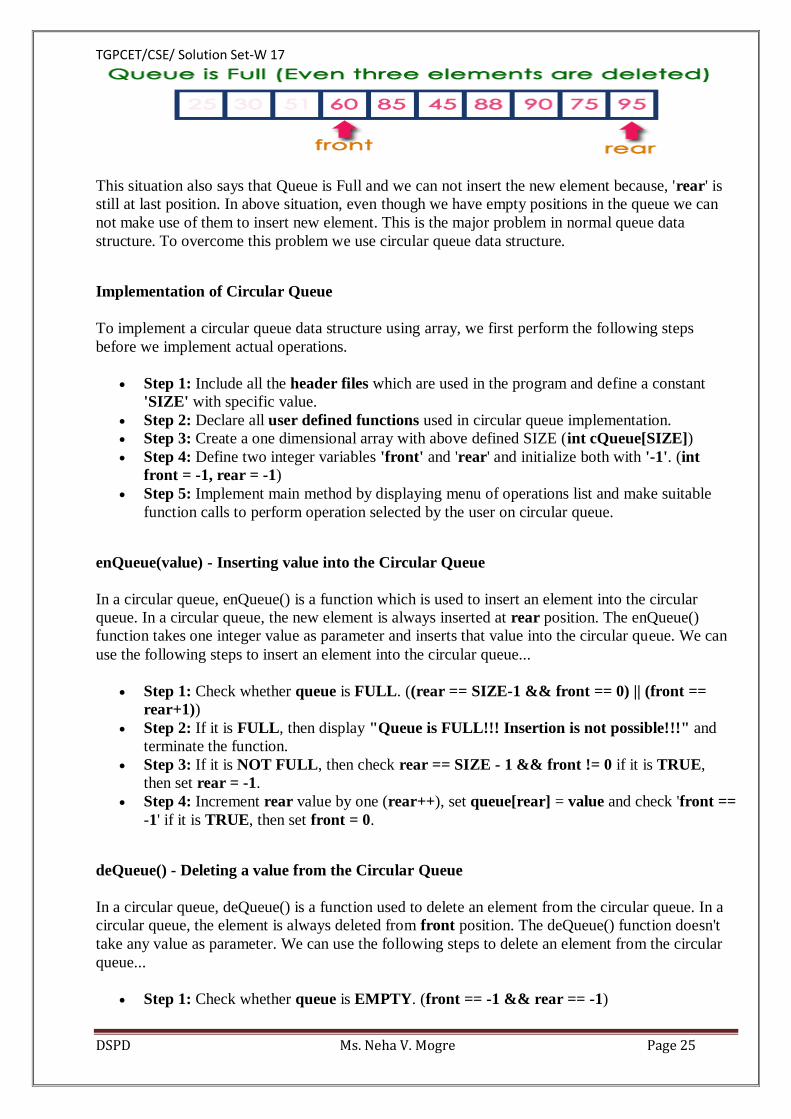
TGPCET/CSE/ Solution Set-W 17
DSPD Ms. Neha V. Mogre Page 25
This situation also says that Queue is Full and we can not insert the new element because, 'rear' is
still at last position. In above situation, even though we have empty positions in the queue we can
not make use of them to insert new element. This is the major problem in normal queue data
structure. To overcome this problem we use circular queue data structure.
Implementation of Circular Queue
To implement a circular queue data structure using array, we first perform the following steps
before we implement actual operations.
Step 1: Include all the header files which are used in the program and define a constant
'SIZE' with specific value.
Step 2: Declare all user defined functions used in circular queue implementation.
Step 3: Create a one dimensional array with above defined SIZE (int cQueue[SIZE])
Step 4: Define two integer variables 'front' and 'rear' and initialize both with '-1'. (int
front = -1, rear = -1)
Step 5: Implement main method by displaying menu of operations list and make suitable
function calls to perform operation selected by the user on circular queue.
enQueue(value) - Inserting value into the Circular Queue
In a circular queue, enQueue() is a function which is used to insert an element into the circular
queue. In a circular queue, the new element is always inserted at rear position. The enQueue()
function takes one integer value as parameter and inserts that value into the circular queue. We can
use the following steps to insert an element into the circular queue...
Step 1: Check whether queue is FULL. ((rear == SIZE-1 && front == 0) || (front ==
rear+1))
Step 2: If it is FULL, then display "Queue is FULL!!! Insertion is not possible!!!" and
terminate the function.
Step 3: If it is NOT FULL, then check rear == SIZE - 1 && front != 0 if it is TRUE,
then set rear = -1.
Step 4: Increment rear value by one (rear++), set queue[rear] = value and check 'front ==
-1' if it is TRUE, then set front = 0.
deQueue() - Deleting a value from the Circular Queue
In a circular queue, deQueue() is a function used to delete an element from the circular queue. In a
circular queue, the element is always deleted from front position. The deQueue() function doesn't
take any value as parameter. We can use the following steps to delete an element from the circular
queue...
Step 1: Check whether queue is EMPTY. (front == -1 && rear == -1)
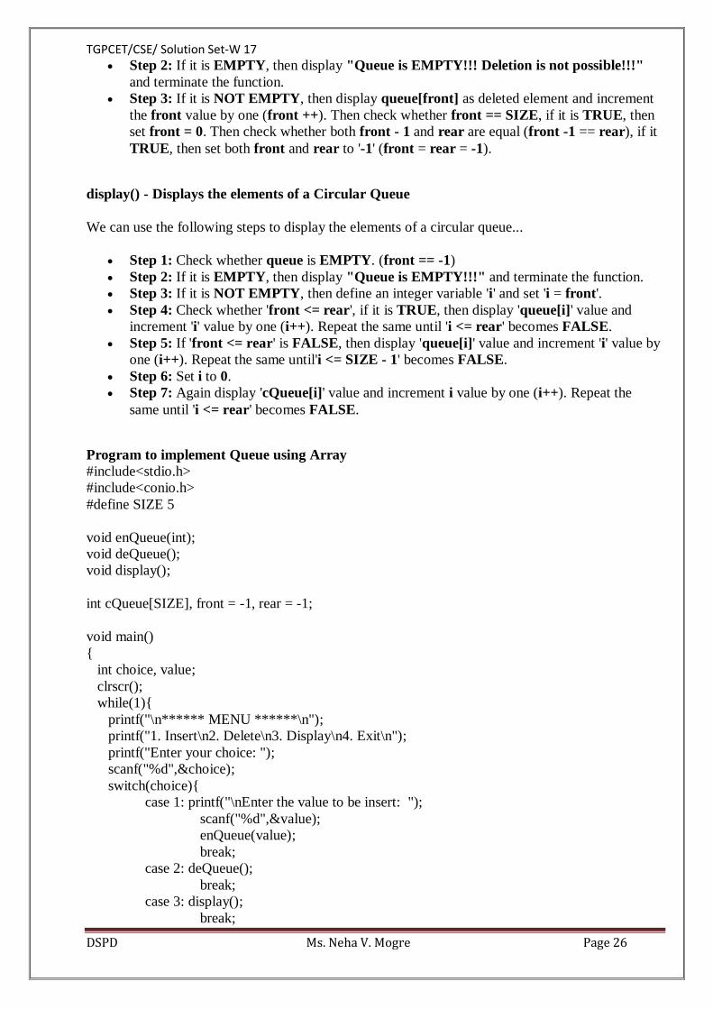
TGPCET/CSE/ Solution Set-W 17
DSPD Ms. Neha V. Mogre Page 26
Step 2: If it is EMPTY, then display "Queue is EMPTY!!! Deletion is not possible!!!"
and terminate the function.
Step 3: If it is NOT EMPTY, then display queue[front] as deleted element and increment
the front value by one (front ++). Then check whether front == SIZE, if it is TRUE, then
set front = 0. Then check whether both front - 1 and rear are equal (front -1 == rear), if it
TRUE, then set both front and rear to '-1' (front = rear = -1).
display() - Displays the elements of a Circular Queue
We can use the following steps to display the elements of a circular queue...
Step 1: Check whether queue is EMPTY. (front == -1)
Step 2: If it is EMPTY, then display "Queue is EMPTY!!!" and terminate the function.
Step 3: If it is NOT EMPTY, then define an integer variable 'i' and set 'i = front'.
Step 4: Check whether 'front <= rear', if it is TRUE, then display 'queue[i]' value and
increment 'i' value by one (i++). Repeat the same until 'i <= rear' becomes FALSE.
Step 5: If 'front <= rear' is FALSE, then display 'queue[i]' value and increment 'i' value by
one (i++). Repeat the same until'i <= SIZE - 1' becomes FALSE.
Step 6: Set i to 0.
Step 7: Again display 'cQueue[i]' value and increment i value by one (i++). Repeat the
same until 'i <= rear' becomes FALSE.
Program to implement Queue using Array
#include<stdio.h>
#include<conio.h>
#define SIZE 5
void enQueue(int);
void deQueue();
void display();
int cQueue[SIZE], front = -1, rear = -1;
void main()
{
int choice, value;
clrscr();
while(1){
printf("\n****** MENU ******\n");
printf("1. Insert\n2. Delete\n3. Display\n4. Exit\n");
printf("Enter your choice: ");
scanf("%d",&choice);
switch(choice){
case 1: printf("\nEnter the value to be insert: ");
scanf("%d",&value);
enQueue(value);
break;
case 2: deQueue();
break;
case 3: display();
break;
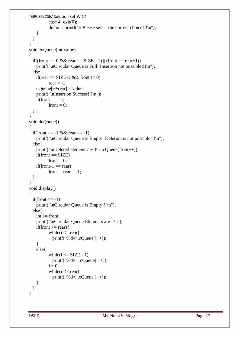
TGPCET/CSE/ Solution Set-W 17
DSPD Ms. Neha V. Mogre Page 27
case 4: exit(0);
default: printf("\nPlease select the correct choice!!!\n");
}
}
}
void enQueue(int value)
{
if((front == 0 && rear == SIZE - 1) || (front == rear+1))
printf("\nCircular Queue is Full! Insertion not possible!!!\n");
else{
if(rear == SIZE-1 && front != 0)
rear = -1;
cQueue[++rear] = value;
printf("\nInsertion Success!!!\n");
if(front == -1)
front = 0;
}
}
void deQueue()
{
if(front == -1 && rear == -1)
printf("\nCircular Queue is Empty! Deletion is not possible!!!\n");
else{
printf("\nDeleted element : %d\n",cQueue[front++]);
if(front == SIZE)
front = 0;
if(front-1 == rear)
front = rear = -1;
}
}
void display()
{
if(front == -1)
printf("\nCircular Queue is Empty!!!\n");
else{
int i = front;
printf("\nCircular Queue Elements are : \n");
if(front <= rear){
while(i <= rear)
printf("%d\t",cQueue[i++]);
}
else{
while(i <= SIZE - 1)
printf("%d\t", cQueue[i++]);
i = 0;
while(i <= rear)
printf("%d\t",cQueue[i++]);
}
}
}
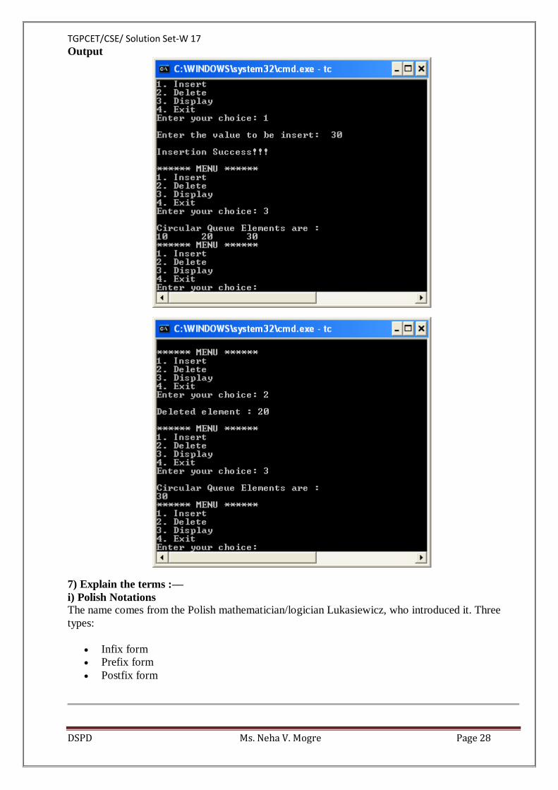
TGPCET/CSE/ Solution Set-W 17
DSPD Ms. Neha V. Mogre Page 28
Output
7) Explain the terms :––
i) Polish Notations
The name comes from the Polish mathematician/logician Lukasiewicz, who introduced it. Three
types:
Infix form
Prefix form
Postfix form

TGPCET/CSE/ Solution Set-W 17
DSPD Ms. Neha V. Mogre Page 29
Infix form
Is exactly the fully parenthesized notation we have just introduced. Let me remind you once again
the Recursive definition
infix-expression := (infix-expression operand infix-expression)
infix-expression := atom
Examples
(3 * 7)
((1 + 3) * 2)
((1 + 3) * ( 2 - 3))
Main Feature: the binary operator is between the two operands.
Question: what if we do not put all the parentheses? Then there are ambiguities on how to interpret
an expression: is 1+2*3 the same as (1+2)*3 or the same as 1+(2*3)? The precedence of operators
solves this problem.
Prefix form
Main Feature: the operator preceeds the two operands.
Recursive definition of fully parenthesized version:
prefix-expression := (operand prefix-expression prefix-expression)
prefix-expression := atom
Recursive definition of classic version, without parentheses (we do not need them, because there is
no longer any ambiguity on how to match the operands to the operators):
prefix-expression := operand prefix-expression prefix-expression
prefix-expression := atom
Examples
(* 3 7) or simply * 3 7
(* ( + 1 3) 2) or simply * + 1 3 2
( * ( + 1 3) ( - 2 3)) or simply * + 1 3 - 2 3
Postfix form
Main Feature: the operator is after the two operands. Recursive definition
postfix-expression := (operand postfix-expression postfix-expression)
postfix-expression := atom
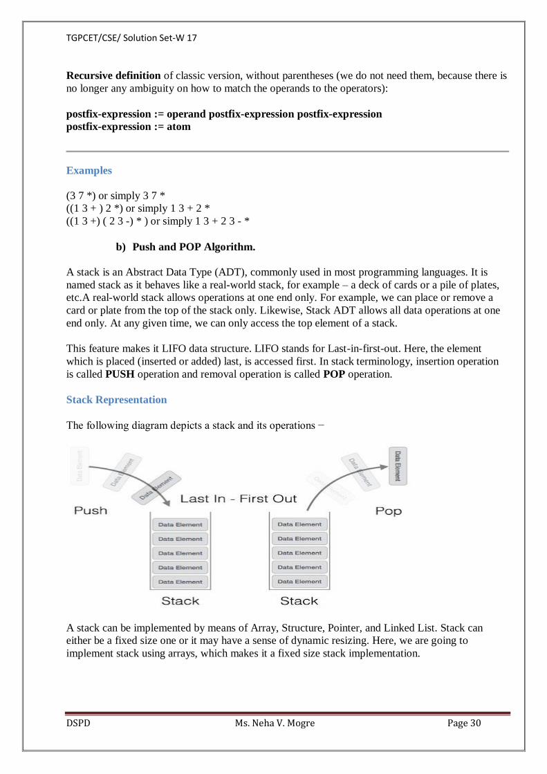
TGPCET/CSE/ Solution Set-W 17
DSPD Ms. Neha V. Mogre Page 30
Recursive definition of classic version, without parentheses (we do not need them, because there is
no longer any ambiguity on how to match the operands to the operators):
postfix-expression := operand postfix-expression postfix-expression
postfix-expression := atom
Examples
(3 7 *) or simply 3 7 *
((1 3 + ) 2 *) or simply 1 3 + 2 *
((1 3 +) ( 2 3 -) * ) or simply 1 3 + 2 3 - *
b) Push and POP Algorithm.
A stack is an Abstract Data Type (ADT), commonly used in most programming languages. It is
named stack as it behaves like a real-world stack, for example – a deck of cards or a pile of plates,
etc.A real-world stack allows operations at one end only. For example, we can place or remove a
card or plate from the top of the stack only. Likewise, Stack ADT allows all data operations at one
end only. At any given time, we can only access the top element of a stack.
This feature makes it LIFO data structure. LIFO stands for Last-in-first-out. Here, the element
which is placed (inserted or added) last, is accessed first. In stack terminology, insertion operation
is called PUSH operation and removal operation is called POP operation.
Stack Representation
The following diagram depicts a stack and its operations −
A stack can be implemented by means of Array, Structure, Pointer, and Linked List. Stack can
either be a fixed size one or it may have a sense of dynamic resizing. Here, we are going to
implement stack using arrays, which makes it a fixed size stack implementation.
TGPCET/CSE/ Solution Set-W 17
DSPD Ms. Neha V. Mogre Page 31
Basic Operations
Stack operations may involve initializing the stack, using it and then de-initializing it. Apart from
these basic stuffs, a stack is used for the following two primary operations −
push() − Pushing (storing) an element on the stack.
pop() − Removing (accessing) an element from the stack.
When data is PUSHed onto stack.
To use a stack efficiently, we need to check the status of stack as well. For the same purpose, the
following functionality is added to stacks −
peek() − get the top data element of the stack, without removing it.
isFull() − check if stack is full.
isEmpty() − check if stack is empty.
At all times, we maintain a pointer to the last PUSHed data on the stack. As this pointer always
represents the top of the stack, hence named top. The top pointer provides top value of the stack
without actually removing it.
First we should learn about procedures to support stack functions −
peek()
Algorithm of peek() function −
begin procedure peek
return stack[top]
end procedure
Implementation of peek() function in C programming language −
Example
int peek() {
return stack[top];
}
isfull()
Algorithm of isfull() function −
begin procedure isfull
if top equals to MAXSIZE
return true
else
return false
endif
TGPCET/CSE/ Solution Set-W 17
DSPD Ms. Neha V. Mogre Page 32
end procedure
Implementation of isfull() function in C programming language −
Example
bool isfull() {
if(top == MAXSIZE)
return true;
else
return false;
}
isempty()
Algorithm of isempty() function −
begin procedure isempty
if top less than 1
return true
else
return false
endif
end procedure
Implementation of isempty() function in C programming language is slightly different. We initialize
top at -1, as the index in array starts from 0. So we check if the top is below zero or -1 to determine
if the stack is empty. Here's the code −
Example
bool isempty() {
if(top == -1)
return true;
else
return false;
}
Push Operation
The process of putting a new data element onto stack is known as a Push Operation. Push operation
involves a series of steps −
Step 1 − Checks if the stack is full.
Step 2 − If the stack is full, produces an error and exit.
Step 3 − If the stack is not full, increments top to point next empty space.
Step 4 − Adds data element to the stack location, where top is pointing.
Step 5 − Returns success.

TGPCET/CSE/ Solution Set-W 17
DSPD Ms. Neha V. Mogre Page 33
If the linked list is used to implement the stack, then in step 3, we need to allocate space
dynamically.
Algorithm for PUSH Operation
A simple algorithm for Push operation can be derived as follows −
begin procedure push: stack, data
if stack is full
return null
endif
top ← top + 1
stack[top] ← data
end procedure
Implementation of this algorithm in C, is very easy. See the following code −
Example
void push(int data) {
if(!isFull()) {
top = top + 1;
stack[top] = data;
} else {
printf("Could not insert data, Stack is full.\n");
}
}
Pop Operation
Accessing the content while removing it from the stack, is known as a Pop Operation. In an array
implementation of pop() operation, the data element is not actually removed, instead top is
decremented to a lower position in the stack to point to the next value. But in linked-list
implementation, pop() actually removes data element and deallocates memory space.
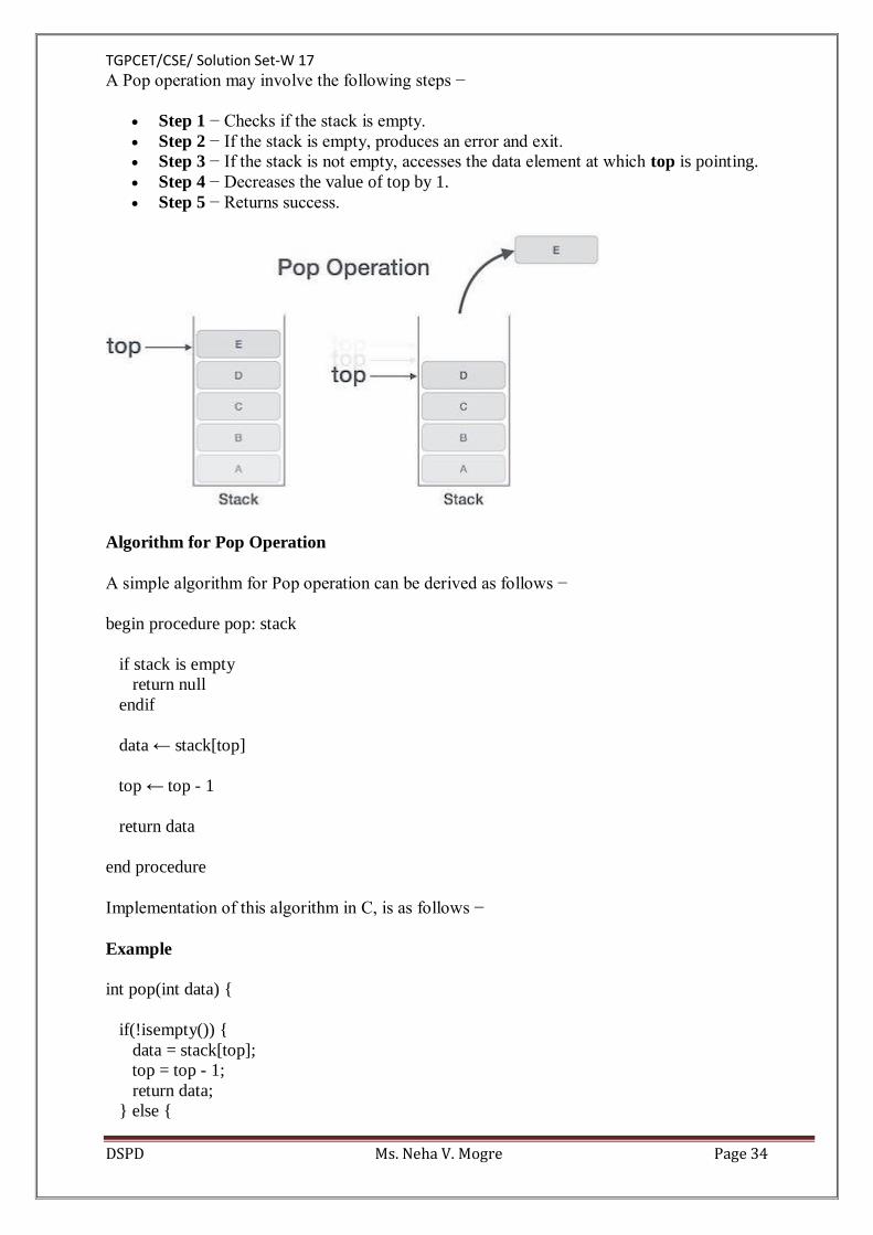
TGPCET/CSE/ Solution Set-W 17
DSPD Ms. Neha V. Mogre Page 34
A Pop operation may involve the following steps −
Step 1 − Checks if the stack is empty.
Step 2 − If the stack is empty, produces an error and exit.
Step 3 − If the stack is not empty, accesses the data element at which top is pointing.
Step 4 − Decreases the value of top by 1.
Step 5 − Returns success.
Algorithm for Pop Operation
A simple algorithm for Pop operation can be derived as follows −
begin procedure pop: stack
if stack is empty
return null
endif
data ← stack[top]
top ← top - 1
return data
end procedure
Implementation of this algorithm in C, is as follows −
Example
int pop(int data) {
if(!isempty()) {
data = stack[top];
top = top - 1;
return data;
} else {

TGPCET/CSE/ Solution Set-W 17
DSPD Ms. Neha V. Mogre Page 35
printf("Could not retrieve data, Stack is empty.\n");
}
}
7 ) What is a Binary Search Tree (BST) ? Make a BST for the following sequence of numbers
: 32, 68, 22, 95, 99, 26, 92, 84, 29, 36 Write Preorder, Inorder and Postorder Traversal
of this Tree.
Binary Search Tree | Set 1 (Search and Insertion)
The following is definition of Binary Search Tree(BST) according to Wikipedia
Binary Search Tree, is a node-based binary tree data structure which has the following properties:
The left subtree of a node contains only nodes with keys less than the node’s key.
The right subtree of a node contains only nodes with keys greater than the node’s key.
The left and right subtree each must also be a binary search tree.
There must be no duplicate nodes.
The above properties of Binary Search Tree provide an ordering among keys so that the operations
like search, minimum and maximum can be done fast. If there is no ordering, then we may have to
compare every key to search a given key.
Searching a key
To search a given key in Bianry Search Tree, we first compare it with root, if the key is present at
root, we return root. If key is greater than root’s key, we recur for right subtree of root node.
Otherwise we recur for left subtree.
// C function to search a given key in a given BST
struct node* search(struct node* root, int key)
{
// Base Cases: root is null or key is present at root
if (root == NULL || root->key == key)
return root;

TGPCET/CSE/ Solution Set-W 17
DSPD Ms. Neha V. Mogre Page 36
// Key is greater than root's key
if (root->key < key)
return search(root->right, key);
// Key is smaller than root's key
return search(root->left, key);
}
Time Complexity: The worst case time complexity of search and insert operations is O(h) where h
is height of Binary Search Tree. In worst case, we may have to travel from root to the deepest leaf
node. The height of a skewed tree may become n and the time complexity of search and insert
operation may become O(n).
Some Interesting Facts:
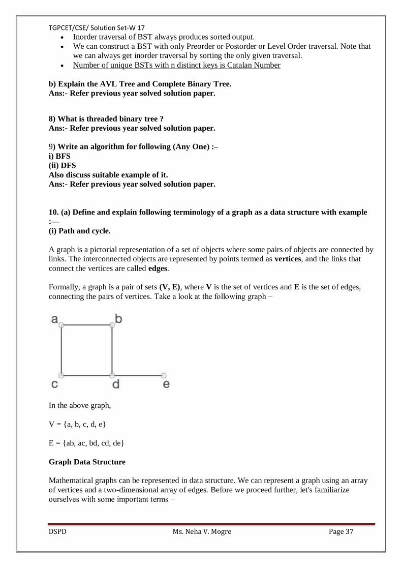
TGPCET/CSE/ Solution Set-W 17
DSPD Ms. Neha V. Mogre Page 37
Inorder traversal of BST always produces sorted output.
We can construct a BST with only Preorder or Postorder or Level Order traversal. Note that
we can always get inorder traversal by sorting the only given traversal.
Number of unique BSTs with n distinct keys is Catalan Number
b) Explain the AVL Tree and Complete Binary Tree.
Ans:- Refer previous year solved solution paper.
8) What is threaded binary tree ?
Ans:- Refer previous year solved solution paper.
9) Write an algorithm for following (Any One) :–
i) BFS
(ii) DFS
Also discuss suitable example of it.
Ans:- Refer previous year solved solution paper.
10. (a) Define and explain following terminology of a graph as a data structure with example
:––
(i) Path and cycle.
A graph is a pictorial representation of a set of objects where some pairs of objects are connected by
links. The interconnected objects are represented by points termed as vertices, and the links that
connect the vertices are called edges.
Formally, a graph is a pair of sets (V, E), where V is the set of vertices and E is the set of edges,
connecting the pairs of vertices. Take a look at the following graph −
In the above graph,
V = {a, b, c, d, e}
E = {ab, ac, bd, cd, de}
Graph Data Structure
Mathematical graphs can be represented in data structure. We can represent a graph using an array
of vertices and a two-dimensional array of edges. Before we proceed further, let's familiarize
ourselves with some important terms −

TGPCET/CSE/ Solution Set-W 17
DSPD Ms. Neha V. Mogre Page 38
Vertex − Each node of the graph is represented as a vertex. In the following example, the
labeled circle represents vertices. Thus, A to G are vertices. We can represent them using an
array as shown in the following image. Here A can be identified by index 0. B can be
identified using index 1 and so on.
Edge − Edge represents a path between two vertices or a line between two vertices. In the
following example, the lines from A to B, B to C, and so on represents edges. We can use a
two-dimensional array to represent an array as shown in the following image. Here AB can
be represented as 1 at row 0, column 1, BC as 1 at row 1, column 2 and so on, keeping other
combinations as 0.
Adjacency − Two node or vertices are adjacent if they are connected to each other through
an edge. In the following example, B is adjacent to A, C is adjacent to B, and so on.
Path − Path represents a sequence of edges between the two vertices. In the following
example, ABCD represents a path from A to D.
Basic Operations
Following are basic primary operations of a Graph −
Add Vertex − Adds a vertex to the graph.
Add Edge − Adds an edge between the two vertices of the graph.
Display Vertex − Displays a vertex of the graph.
B) Shortest Path Problem
Shortest paths.
An edge-weighted digraph is a digraph where we associate weights or costs with each edge. A
shortest path from vertex s to vertex t is a directed path from s to t with the property that no other
such path has a lower weight.
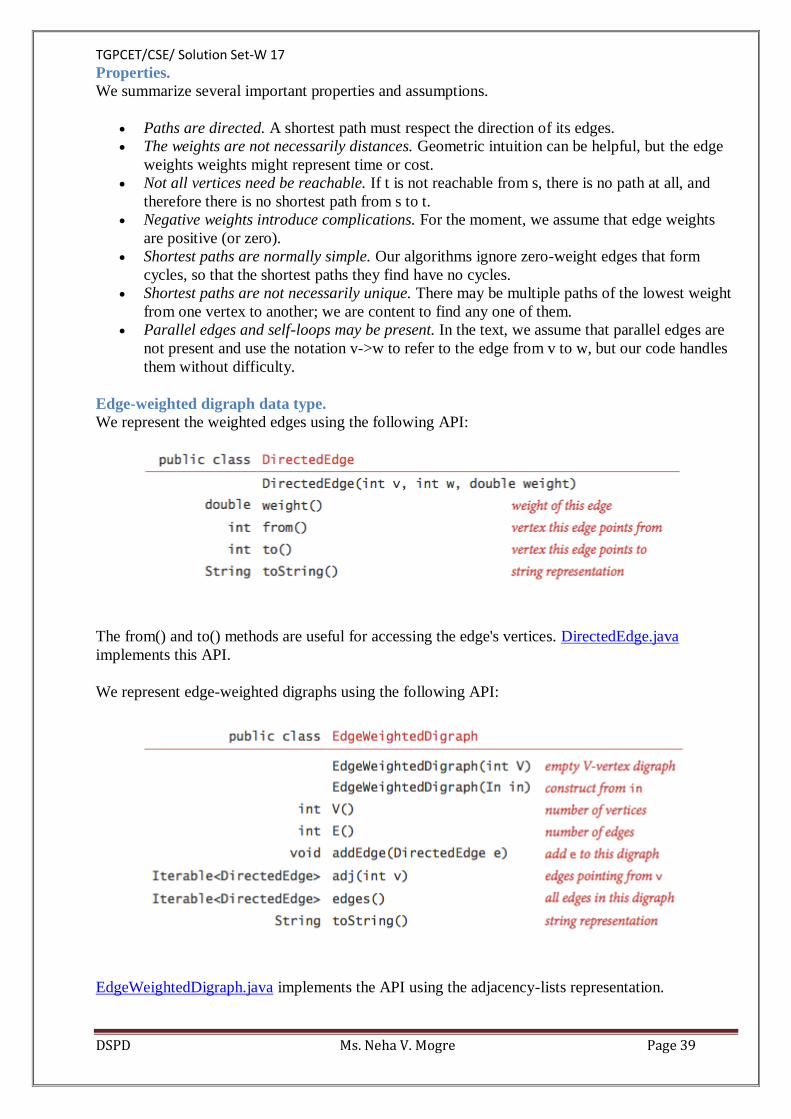
TGPCET/CSE/ Solution Set-W 17
DSPD Ms. Neha V. Mogre Page 39
Properties.
We summarize several important properties and assumptions.
Paths are directed. A shortest path must respect the direction of its edges.
The weights are not necessarily distances. Geometric intuition can be helpful, but the edge
weights weights might represent time or cost.
Not all vertices need be reachable. If t is not reachable from s, there is no path at all, and
therefore there is no shortest path from s to t.
Negative weights introduce complications. For the moment, we assume that edge weights
are positive (or zero).
Shortest paths are normally simple. Our algorithms ignore zero-weight edges that form
cycles, so that the shortest paths they find have no cycles.
Shortest paths are not necessarily unique. There may be multiple paths of the lowest weight
from one vertex to another; we are content to find any one of them.
Parallel edges and self-loops may be present. In the text, we assume that parallel edges are
not present and use the notation v->w to refer to the edge from v to w, but our code handles
them without difficulty.
Edge-weighted digraph data type.
We represent the weighted edges using the following API:
The from() and to() methods are useful for accessing the edge's vertices. DirectedEdge.java
implements this API.
We represent edge-weighted digraphs using the following API:
EdgeWeightedDigraph.java implements the API using the adjacency-lists representation.
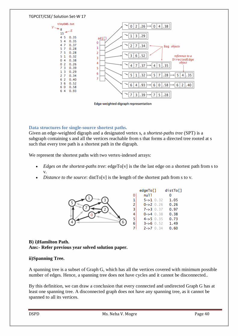
TGPCET/CSE/ Solution Set-W 17
DSPD Ms. Neha V. Mogre Page 40
Data structures for single-source shortest paths.
Given an edge-weighted digraph and a designated vertex s, a shortest-paths tree (SPT) is a
subgraph containing s and all the vertices reachable from s that forms a directed tree rooted at s
such that every tree path is a shortest path in the digraph.
We represent the shortest paths with two vertex-indexed arrays:
Edges on the shortest-paths tree: edgeTo[v] is the the last edge on a shortest path from s to
v.
Distance to the source: distTo[v] is the length of the shortest path from s to v.
B) i)Hamilton Path.
Ans:- Refer previous year solved solution paper.
ii)Spanning Tree.
A spanning tree is a subset of Graph G, which has all the vertices covered with minimum possible
number of edges. Hence, a spanning tree does not have cycles and it cannot be disconnected..
By this definition, we can draw a conclusion that every connected and undirected Graph G has at
least one spanning tree. A disconnected graph does not have any spanning tree, as it cannot be
spanned to all its vertices.
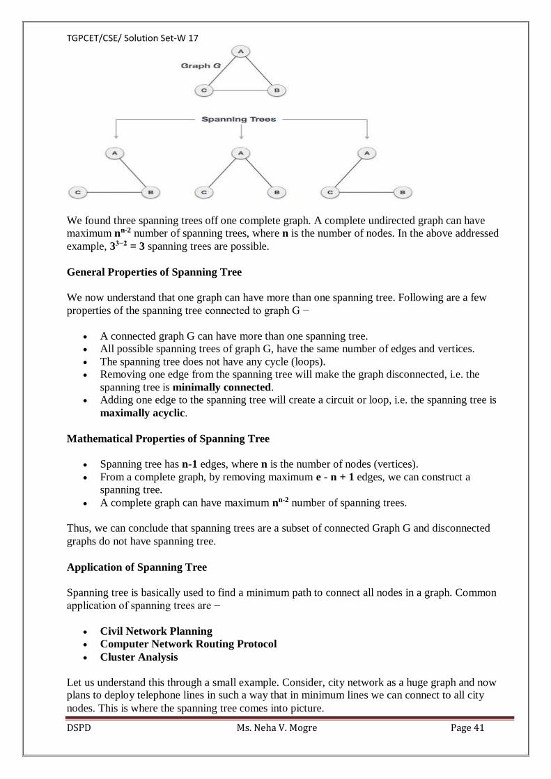
TGPCET/CSE/ Solution Set-W 17
DSPD Ms. Neha V. Mogre Page 41
We found three spanning trees off one complete graph. A complete undirected graph can have
maximum nn-2 number of spanning trees, where n is the number of nodes. In the above addressed
example, 33−2 = 3 spanning trees are possible.
General Properties of Spanning Tree
We now understand that one graph can have more than one spanning tree. Following are a few
properties of the spanning tree connected to graph G −
A connected graph G can have more than one spanning tree.
All possible spanning trees of graph G, have the same number of edges and vertices.
The spanning tree does not have any cycle (loops).
Removing one edge from the spanning tree will make the graph disconnected, i.e. the
spanning tree is minimally connected.
Adding one edge to the spanning tree will create a circuit or loop, i.e. the spanning tree is
maximally acyclic.
Mathematical Properties of Spanning Tree
Spanning tree has n-1 edges, where n is the number of nodes (vertices).
From a complete graph, by removing maximum e - n + 1 edges, we can construct a
spanning tree.
A complete graph can have maximum nn-2 number of spanning trees.
Thus, we can conclude that spanning trees are a subset of connected Graph G and disconnected
graphs do not have spanning tree.
Application of Spanning Tree
Spanning tree is basically used to find a minimum path to connect all nodes in a graph. Common
application of spanning trees are −
Civil Network Planning
Computer Network Routing Protocol
Cluster Analysis
Let us understand this through a small example. Consider, city network as a huge graph and now
plans to deploy telephone lines in such a way that in minimum lines we can connect to all city
nodes. This is where the spanning tree comes into picture.

TGPCET/CSE/ Solution Set-W 17
DSPD Ms. Neha V. Mogre Page 42
Minimum Spanning Tree (MST)
In a weighted graph, a minimum spanning tree is a spanning tree that has minimum weight than all
other spanning trees of the same graph. In real-world situations, this weight can be measured as
distance, congestion, traffic load or any arbitrary value denoted to the edges.
Minimum Spanning-Tree Algorithm
We shall learn about two most important spanning tree algorithms here −
Kruskal's Algorithm
Prim's Algorithm
Both are greedy algorithms.
11A)What is collision in hashing ? How can it be avoided ? What are the different collision
handling mechanisms ? Explain each with suitable example
Ans:- Refer previous year solved solution paper.
12) What is symbol table ? What are different data structures used for symbol table ? Discuss.
In computer science, a symbol table is a data structure used by a language translator such as a
compiler or interpreter, where each identifier in a program's source code is associated with
information relating to its declaration or appearance in the source.
Implementation
A common implementation technique is to use a hash table. A compiler may use one large symbol
table for all symbols or use separated, hierarchical symbol tables for different scopes. There are also
trees, linear lists and self-organizing lists which can be used to implement a symbol table. It also
simplifies the classification of literals in tabular format. The symbol table is accessed by most
phases of a compiler, beginning with the lexical analysis to optimization.
Uses
An object file will contain a symbol table of the identifiers it contains that are externally visible.
During the linking of different object files, a linker will use these symbol tables to resolve any
unresolved references.
A symbol table may only exist during the translation process, or it may be embedded in the output
of that process for later exploitation, for example, during an interactive debugging session, or as a
resource for formatting a diagnostic report during or after execution of a program.
While reverse engineering an executable, many tools refer to the symbol table to check what
addresses have been assigned to global variables and known functions. If the symbol table has been
stripped or cleaned out before being converted into an executable, tools will find it harder to
determine addresses or understand anything about the program.
At that time of accessing variables and allocating memory dynamically, a compiler should perform
many works and as such the extended stack model requires the symbol table.
Example

TGPCET/CSE/ Solution Set-W 17
DSPD Ms. Neha V. Mogre Page 43
Consider the following program written in C:
// Declare an external function
extern double bar(double x);
// Define a public function
double foo(int count)
{
double sum = 0.0;
// Sum all the values bar(1) to bar(count)
for (int i = 1; i <= count; i++)
sum += bar((double) i);
return sum;
}
A C compiler that parses this code will contain at least the following symbol table entries:
Symbol name Type Scope
bar function, double extern
x double function parameter
foo function, double global
count int function parameter
sum double block local
i int for-loop statement
In addition, the symbol table will also contain entries generated by the compiler for intermediate
expression values (e.g., the expression that casts the i loop variable into a double, and the return
value of the call to function bar()), statement labels, and so forth.
As another example, the symbol table of a small program is listed below. The table itself was
generated using the GNU binutils' nm utility. There is one data symbol, (noted by the "D" type),
and many functions (self defined as well as from the standard library). The first column is where the
symbol is located in the memory, the second is "The symbol type" and the third is the name of the
symbol. By passing suitable parameters, the symbol table was made to sort on basis of address.
Top Related