


Languages
Pages
Legal


Jeffrey F. Williamson, Ph.D.
Monte Carlo and Experimental Dosimetry of Low-energy Brachytherapy Sources
Jeffrey F. Williamson, Ph.D. Virginia Commonwealth University
Mark R. Rivard, Ph.D.Tufts-New England Medical Center
Quantitative Dosimetry Methods for Brachytherapy
AAPM Summer School19 July 2005
Virginia Commonwealth UniversityVCU Radiation Oncology

What is “Quantitative Dosimetry?”
• Williamson’s definition: absorbed dose estimation method providing
– Accurate representation of well-defined physical quality– Rigorous uncertainty analysis ⇒ <10% uncertainty 0.5 to
5 cm in liquid water – Traceable to NIST primary standards (SK,N99)
• Applications– Single-source dose-rate arrays for TG-43 parameter
determination (“Reference quality” dose distributions)– Direct treatment planning– Validating semi-empirical algorithms

Outline
• Experimental Techniques– TLD dosimetry: current standard of practice– Emerging experimental techniques
• Monte Carlo-based dosimetry• Results of TLD and MC dosimetry
– Uncertainty analysis– Agreement

Quantitative Dosimetry Era: 1980-• 1955 Tochlin: Film Dosimetry• 1966 Lin & Kenny: TLD dosimetry in
medium• 1983 Ling: Diode dosimetry of I-125
seeds• 1985 Loftus: I-125 exposure standard• 1986 NIH ICWG contract
– Nath, Anderson, Weaver: Validation of TLD dosimetry
• 1983 Williamson: Monte Carlo dosimetry• 1994 Task Group 43 Report

TLD dose measurements around 226Ra NeedleLin and Cameron: Univ. of Wisconsin, 1965

Dosimetric Environment• Large Dose Gradients
– Wide Range of Dose Rates– Positioning accuracy needed for 2 % dose
accuracy 2 mm Distance ±20 μm5 mm Distance ±50 μm
10 mm Distance ±100 μm– Large Number of Measurements Needed
• Low Photon Energies• Relatively Low Dose Rates

Criteria for experimental dosimeters
• Signal stability and reproducibility– Spatially and temporally constant Sensitivity (signal/dose) – Free of fading, dose-rate effects– Good signal-to-noise ratio (SNR)
• Small size, high sensitivity, large dynamic range– Small size: avoid averaging dose gradients– Large size: Good signal at low doses
• Good positioning accuracy• Support measurements at many points

Sensitivity (10 cm)/Sensitivity (1 cm) vs energy
0.75
1.00
1.25
1.50
1.75
2.00
2.25
2.50
100 1000
LiF TLDPolyvinyl TolueneSilicon diode
Sens
itivi
ty (r
eadi
ng/D
wat
): 1
0 cm
/1 c
m
Energy (KeV)20 200 500

Localization via Digital Dosimeters
X Axis (mm)
Y A
xis
(mm
)
2D dose distribution
10 20 30 40 50 60 70
10
20
30
40
50
60
70
A
B
Yc
Xc10 20 30 40 50 60 70
10
20
30
40
50
60
X Axis (mm)
Dos
e (G
y)
Profile A
Xc = (X2 -X1)/2
X1 X2Xc
30-100 μm positional accuracy achievable

Solid Water Phantoms for TLD Dosimetry
Transverse Axis Measurement Phantom
90 o
60 o
45 o
20 o
0 o
120 o
135 o
160 o
180 o
Polar Dose Profile Measurement Phantom
100-200 μm positional accuracy achievable

TLD Detectors• Use TLD-100 LiF extruded ribbons (‘chips’)
1 x 1 x 1 mm3 at distances < 2 cm3 x 3 x 0.9 mm3 at distances ≥ 2 cm
• Use RMI 453 Machined Solid Water Phantom– Composition (CaCO3 + organic foam) not stable– Either perform chemical assay or use high purity PMMA
• Annealing protocol1 hour 400° C followed by 24 hours of 80° C pre-irradiation
OR1 hour 400° C pre-irradiation followed by 10 minutes at 100°
C Post-irradiation

Brachytherapy Dosimetry
• Given: Relative solid state dosimeter reading (TLD or Diode)
• Desired: absorbed dose to water
• Corrected for:– Detector sensitivity– Measurement vs reference geometry– Radiation field Perturbation – Detector response artifacts
Solid Water Phantom
Detector at (x,y,z)
Source
Dose rate to Water at (x,y,z)
Liquid Water Reference Sphere
Dwat (r r )
Rdet (r r )

Brachytherapy Dose Measurement
is measured Response in calibration beam, λ
is relative detector response at in Brachytherapy geometry
BRx
wat det
K Kmeas
D (r ) R (r ) g(T)S S E(r )λ
⎡ ⎤ ⋅=⎢ ⎥ ⋅ ε ⋅⎣ ⎦
r r&r
ελ = Rdet Dmed[ ]measλ
E(r r ) =Rdet Dwat[ ]BRx at r r
ελ
r r
• SK = Measured Air-Kerma Strength• g(T) = 1/effective exposure time (decay correction)

TLD readings
• TLi is Measured Response of i-th detector at r
• Flin(TL) is non-linearity correction for net response TL
• Si is relative sensitivity of i-th detector derived from reading TLDs exposed to uniform doses
• TG-43 recommends n = 5-15
n i bkgdTLD
lin ii 1
(TL TL )R (r) 1/ n
F S=
−=
⋅∑r

Relative Energy Response
[ ][ ]
wat
med
BRx 00
0
TL(r) / D (r) for Brachy SourceE(r)
TL / D for Calibration Beam(TL ,r) for same TL(TL )λ
=λ
ε=
ε
r rr
r
• E(d) obtained by– Measuring TLD response in free air as function of
average energy in low energy x-ray beams– Monte Carlo calculations– Analytic calculations
• Generally assumed to be independent of position

Compare detector to “matched”X-ray Beam calibration in Free-Air
hυ = 40-120 kVp
ted ion chamber Scintillator Detector
( )
FSair
h hair wat MC
FS repl dispair Meas
TL TLD mean net reading
K measured air kerma
K DTLE(r)c c (r)K
ν ν
λ
=
=
⎛ ⎞= ⋅⎜ ⎟⎜ ⎟ ⋅ ⋅ ε⎝ ⎠
watrepl FS
wat
disp wat watV(r)
D in mediumc 0.97K in cavity
1c (r) D (r) at point D (r')dV' (0.80 1.00)V(r)
=
⎡ ⎤⎢ ⎥= ∈ −⎢ ⎥⎣ ⎦
∫r
r rr

Measured E factors
• Conventional choice: E=1.4 w/o regard to details• Hence, 2004 TG-43 has assigned 5% uncertainty to E
0.9
1.0
1.1
1.2
1.3
1.4
1.5
101 102 103 104
Best fit lineReft 1988Muench 1991Hartmann 1983Weaver 1984Meigooni 1988b
0.9
1.0
1.1
1.2
1.3
1.4
1.5
Photon energy (KeV)
Rel
ativ
e En
ergy
Res
pons
e

Monte Carlo Evaluation of E(d)• E(d) Corrects for
– Measurement medium and geometry vs water – Calibration medium vs. water– Detector artifacts: Energy response, volume averaging,
angular anisotropy, self attenuation • Assume: Detector response energy imparted to
active volume for beam qualities λ
[ ][ ]
MCBRx
MC
det det
det wat
det med
If R D
D (r) / D (r)Then E(r)
D / D λ
λ λ= α ⋅
Δ Δ=
Δ Δ
r rr

Measured vs. Calculated E(d) Davis 2003 and Das 1995
Energy linearity of TLD is controversial
0.90
0.95
1.00
1.05
1.10
1.15
10 100 1000
Davis (3x3x0.4 mm3)Das (3x3x0.9 mm3)Das (1x1x1 mm3)R
elat
ive
Ener
gy R
espo
nse
Mea
sure
d/M
onte
Car
lo
Photon Energy (keV)
( )( )
air
air Meas
TLD air MC
R TL at energy
K measured air kerma
TL K
D K
λλ
λ
λ λ
= λ
=
α =

I-125 Seed E(d) in Solid Water
1.05
1.15
1.25
1.35
1.45
0 1 2 3 4 5
LiF Point Detector
1x1x1 mm3 TLD-100
1x1x1 mm3 TLD-100Rel
ativ
e En
ergy
Res
pons
e: E
(d)
Distance (cm), d
⎧⎨⎩
Chemical Analysis: 1.6% Ca
RMI Specifications: 2.3% Ca {
• Solid-to-Liquid Water correction: 4%-15% at 1-5 cm • 10-30% variations in SW composition reported: 5%-20%
dosimetric errors

Summary: TLD phantom dosimetry
• 1-3 mm size ⇒ precision: 2-5% above 1 cGy• Energy response corrections
– Distance independent, excluding phantom corrections– Energy linearity is controversial (<10%)– Many corrections routinely ignored
• Widely-used SW phantom has uncertain composition– High-purity industrial plastics recommended
• Extensive benchmarking of TLD vs Monte Carlo – 3-10% agreement for Pd-103 and I-125 sources– 7%-10% absolute dose measurement uncertainty

Other dosimetry systems
• Plastic scintillator (PS) and diode probes– High sensitivity, small size, good SNR, and waterproof– Single element detectors requiring water scanning system
• PS: established as transfer/relative dosimeter for beta sources
» Large (30%) energy nonlinearity• Diode: underutilized in presenter’s opinion
– Energy linearity well established– Large E(d) variation for medium energy sources– Well established as relative dosimeter

Emerging Dosimetry Systems2D RadioChromic Film
Ir-192 HDR Source

Absolute RCF Dose Measurement vs
Monte CarloHDR 192Ir Source
RCF 2σ uncertainty: 4.6%
-5 -4 -3 -2 -1 00.95
1
1.05
Away [cm]
Dos
e [G
y]

Absolute RCF dosimetry for LDR SourcesCs-137: RCF/MC vs. Exposure-to-densitometry
time interval
• Mean error vs dose• 6 day exposure• Very high 100 μm
spatial resolution• Fading artifacts not
significant• Energy linearity
within 5%

Monte Carlo Simulation Typical Trajectory
Heterogeneity
Photon Collision
Ti capsuleScoring Bin, ΔV
I-125 Seed
Ag coreAg core
(r0,Ω0,E 0,W0) Ω0,E0
(r1,Ω1,E1,W1) →r1
Ω1,E1
Ω3,E3
r3 Ω2,E2

Monte Carlo Technical IssuesMonte Carlo Technical Issues
Particle Collision DynamicsTotal and differential cross sections for all collision processes and media
Particle Collision DynamicsTotal and differential cross sections for all collision processes and media
Geometric ModelSize, location, shape, composition and topology
of each material object
Geometric ModelSize, location, shape, composition and topology
of each material object
Detector Model relationship between dose and collision density
Detector Model relationship between dose and collision density

Collisional Physics Requirements for Low-Energy Brachytherapy
• Only photon transport needed– Secondary CPE obtains (Dose ≈ Kerma)– Neutral-particle variance reduction techniques useful
• Comprehensive model of photon collisions– NIST EXCOM or EPDL97 Cross sections are essential!!– Coherent scattering and electron binding corrections
» Use molecular/condensed medium form factors– Characteristic x-ray emission from photo effect– Approximations OK for some RTP applications
• Options: MCNP, EGSnrc and VCU’s PTRAN_CCG

Geometric Model Validation
DraxImage I-125 Seed
Contact Radiograph Final Model
6711 silver rod endElectron microscopy
6711 contact radiographs
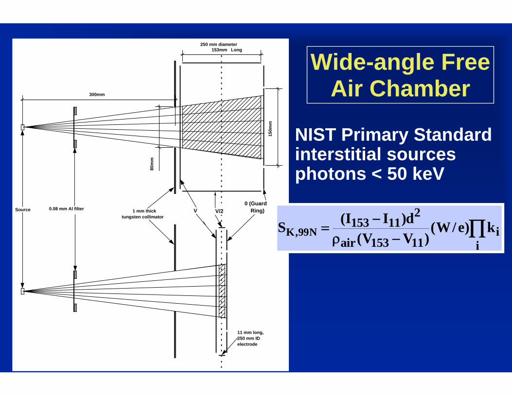
Wide-angle FreeAir Chamber
NIST Primary Standardinterstitial sourcesphotons < 50 keV
V V/20 (Guard Ring)
300mm
80m
m
150m
m
153mm
1 mm thick tungsten collimator
250 mm diameterLong
Source
11 mm long, 250 mm ID electrode
0.08 mm Al filter
K,99N
2153 11
iair 153 11 i
(I I )dS (W/e) k(V V )
−=ρ − ∏

Analog and Tracklength Dose Estimation
=
Δ∝ ⋅
2,3
1,41,4 n
3 3
D
Energy in - Energy out from n+1voxel mass
sD from n E
vo
Need cubic array of voxels: 1x1x1 mm to 2x2x2 mm
Analogue Estimator (EGS method)
Expected Value Tracklength Estimator
( )⋅ μ ρenxel volume
rn
rn+1
( ,E )Ωn n
( )Ωn+1 n+1,E
j=1 2 3
4
S1,4ΔS1,4

Estimator Use• Tracklength estimators
– 20-50X more efficient than analog– Models volume averaging and medium replacement by
extended detectors– 3D patient (voxel array) calculations
• Next flight estimators: dose-at-a-point– Condensed-medium dose calculations at least 1-2 mm
from interfaces– Dilute-medium (air) kerma calculations– 0.1% - 2% statistical precision for I-125 dosimetry
• Kalli/Cashwell “Once-more-collided Flux”– Point doses near media interfaces– Energy imparted to small detectors

Monte Carlo quantities for typical seed study
{wat
ab
Bounded next-flight estimator for most distances
Transverse axisD (cGy/simulated photon): angular dose profiles
E Energy imparted to WAFAC volume/simulated photon Track -leng
Δ
Δ
air
th estimator when fluence varies over detector Next-flight point dose estimator for TLD/dio
Transverse-axis at geometric points
de detectors > 2 cm from s
K in free ai
ource
r angΔ { Track length for WAFAC Next-flight for tr
ular fluence pr
ansverse axis
ofile (
distrib
30 cm)
ution

Calculation of TG-43 Parameters by MCPT
Calculation of TG-43 Parameters by MCPT
MCPT calculates per disintegration within source:- Dose to medium, ΔDmed(r), near source in phantom
geometry: usually 30 cm liquid water sphere- Air-kerma strength, ΔSK, in free-air geometry usually
5 m air sphere or detailed model of calibration vault
watK
watwat
D (r 1 cm, / 2)S
D (r, / 2) G(1 cm, / 2)g(r)D (1 cm, / 2) G(r, / 2)
Δ = θ = πΛ =
Δ
Δ π ⋅ π=Δ π ⋅ π

Calculation of ΔSKExtrapolated Point-Kerma method
• Place sealed source model at center of large air sphere• Calculate air-kerma/disintegration, ΔKair(d), as function
transverse axis distance, d• Extrapolate to free-space geometry by curve fitting
Where ΔSK and α are unknowns(1 + αd) - SPR accounts for scatter buildupμ = primary photon attenuation coefficient
2 dair KK (d) d S (1 d) e−μΔ ⋅ = Δ ⋅ + α ⋅&

Models 200 (103Pd), 6702 (125I) and 6711 (125I) Seeds
4.50
0 0.826 0.612
3.14
0
0.89
0
0.560
1.09
0
0.510
Graphite pelletPb marker
3.50
0
4.50
0
2.20
0
0.60
0
0.700 0.800
Ti CapsuleResin spheres
3.50
0
4.50
0
0.700 0.800
3.00
0
0.500
Ag RodAg-halide layer
• Model 200– 103Pd distributed in
thin (2-25 μm) Pd metal coating of right circular graphite cylinder
• Model 6702– 125I distributed on
surface of radio transparent resin spheres
• Model 6711– 125I distributed in thin
(≈3 μm) silver-halide coating of right circular Ag cylinder

Sharp corners and opaque coatings
Thin High-density coating
Low-density core
High-density cylinder
Low-density core
Near transverse-axis:Anisotropic at long distancesIsotropic at short distancesInverse square-law deviations
Anisotropic at long and short distances
1
Circular ends contribute at 8 d 1 cmLtan
2 d 0.3 d 30 cm− ° =⎧⎡ ⎤θ = = ⎨⎢ ⎥× ° =⎣ ⎦ ⎩
Isotropic at both long and short distances

Polar Anisotropy in Air (30 cm)
0.00
0.25
0.50
0.75
1.00
1.25
0 10 20 30 40 50 60 70 80 90
Model 6702 I-125
Model 6711 I-125
Model 200 Pd-103
Pola
r Kai
r pro
file
(30
cm in
air)
Polar angle (degrees)

ΔSK: Point-Extrapolation Method
0.40
0.50
0.60
0.70
0.80
0.90
1.00
1.10
1.20
0 20 40 60 80 100
Model 200 ( 2 μm Pd) Pd-103 Model 6702 I-125 Model 6711 I-125
ΔK
air(d
) ⋅ d
2
cGy⋅
cm2 ⋅h
-1/(m
Ci⋅h
)
Distance (cm)
Data Points: MCPTSolid Lines: Fit

‘WAFAC:’ Wide Angle Free-Air Chamber
Rotating Seed Holder
V
V/2
0 (Guard Ring)
300mm
80m
m
150m
m
153mm
1 mm thick tungsten collimator
250 mm diameterLong
Source
Collecting volume
I
0.08 mm Al filter
100mm

WAFAC Simulation Method153 11 2ab ab
K inv attair 153 11
( E E ) dS k k(V V )
Δ − Δ ⋅Δ = ⋅ ⋅
ρ ⋅ −
( ) {
xab
K extratt 2
inv WFC
inv
where E Energy absorbed/disintegration in WAFAC volume of length xd 38 cm seed-to-WAFAC volume center
( S ) 1.025 Pd-103k for a point source 1.013 I-125k K d
k inverse squa
Δ =
= =
⎫Δ ⎪= =⎬
⋅ Δ ⋅ ⎪⎭
= − A( ) dA
re correction 1.0089(d) A
Φ ⋅= =
Φ ⋅
∫ l
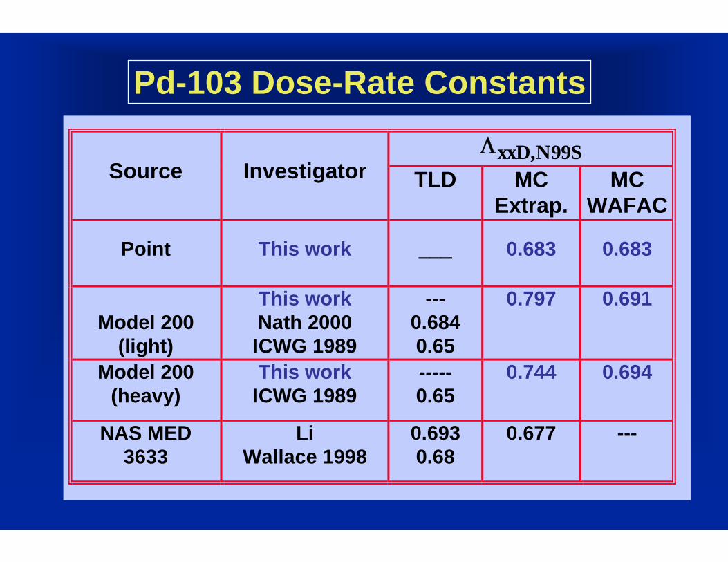
Pd-103 Dose-Rate Constants
xxD,N99SΛ Source
Investigator TLD MC
Extrap.MC
WAFAC
Point
This work
___
0.683
0.683
Model 200
(light)
This work Nath 2000 ICWG 1989
--- 0.684 0.65
0.797 0.691
Model 200 (heavy)
This work ICWG 1989
----- 0.65
0.744 0.694
NAS MED 3633
Li Wallace 1998
0.693 0.68
0.677 ---

Monte Carlo vs. TLD: 125I Seeds• 14 Seed models, 38 Candidate datasets
0.4
0.6
0.8
1.0
1.2
1.4
1.6
0 2 4 6 8 10
distance, r [cm]
dose
-rat
e ra
tios,
Mon
te C
arlo
/ ex
perim
enta
l

Monte Carlo/TLD Dose Rates: 125I Seeds

Monte Carlo/TLD Dose Rates: 125I Seeds

TLD and Monte Carlo Uncertainty Analysis

Monte Carlo vs TLD
• Measurement Pros and Cons– Large uncertainties and many artifacts– Tests conjunction of all a priori assumptions: seed
geometry, detector response corrections, etc• Monte Carlo Pros and Cons
– Artifact free and low uncertainty– Garbage in-Garbage out
» Seed geometry errors» Will not anticipate contaminant radionuclides etc.,
SK errors– Does not model detector signal formation

Conclusions
• Low energy brachytherapy: main catalyst for improving dosimetry and source standardization for 30 years
– Single-source dose distributions have 5% uncertainty– Both MC and measurement have important roles
• Current Role– Monte Carlo: primary source of dosimetric data– Measurement: Confirm assumptions underlying Monte
Carlo model• Major needs: more accurate and efficient dose-
measurement systems for low energy sources– Test source-to-source variations during manufacturing
process
Top Related