


Languages
Pages
Legal

December 2010Jeffrey W. BermanBo-Shiuan WangCharles W. RoederAaron W. OlsonDawn E. Lehman
WA-RD 757.1
Office of Research & Library Services
WSDOT Research Report
Triage Evaluation ofGusset Plates inSteel Truss Bridges

Research Report Research Project T4118, Task 44
Gusset Plates
December 2010
TRIAGE EVALUATION OF GUSSET PLATES IN STEEL TRUSS BRIDGES
by
Jeffrey W. Berman Assistant Professor
Bo-Shiuan Wang Graduate Research Assistant
Charles W. Roeder Professor
Aaron W. Olson Graduate Research Assistant
Dawn E. Lehman Associate Professor
Department of Civil and Environmental Engineering University of Washington, Box 352700
Seattle, Washington 98195
Washington State Transportation Center (TRAC) University of Washington, Box 354802
University District Building 1107 NE 45th Street, Suite 535
Seattle, Washington 98105-4631
Washington State Department of Transportation Technical Monitor Harvey Coffman
Bridge Preservation Engineer, Bridge and Structures Division
Prepared for
The State of Washington Department of Transportation
Paula J. Hammond, Secretary

TECHNICAL REPORT STANDARD TITLE PAGE
1. REPORT NO. 2. GOVERNMENT ACCESSION NO. 3. RECIPIENT'S CATALOG NO.
WA-RD 757.1 4. TITLE AND SUBTITLE 5. REPORT DATE
TRIAGE EVALUATION OF GUSSET PLATES IN STEEL TRUSS BRIDGES
December 2010 6. PERFORMING ORGANIZATION CODE
7. AUTHOR(S) 8. PERFORMING ORGANIZATION REPORT NO.
Jeffrey W. Berman, Bo-Shiuan Wang, Charles W. Roeder, Aaron W. Olson, Dawn E. Lehman 9. PERFORMING ORGANIZATION NAME AND ADDRESS 10. WORK UNIT NO.
Washington State Transportation Center (TRAC) University of Washington, Box 354802 University District Building; 1107 NE 45th Street, Suite 535 Seattle, Washington 98105-4631
11. CONTRACT OR GRANT NO.
Agreement T4118, Task 44
12. SPONSORING AGENCY NAME AND ADDRESS 13. TYPE OF REPORT AND PERIOD COVERED
Research Office Washington State Department of Transportation Transportation Building, MS 47372 Olympia, Washington 98504-7372 Project Manager: Kim Willoughby, 360.705.7978
Final Research Report 14. SPONSORING AGENCY CODE
15. SUPPLEMENTARY NOTES
This study was conducted in cooperation with the U.S. Department of Transportation, Federal Highway Administration. 16. ABSTRACT:
Following research into the collapse of the I-35W steel truss bridge in Minneapolis, Minnesota, FHWA released recommendations for load rating the gusset plates of steel truss bridges. The recommendations include evaluation of several limit states, one of which requires the consideration of multiple load cases and possible lines failure, making the procedures somewhat difficult and time consuming to employ. Given the large inventory of steel truss bridges in Washington state and around the country, and the large number of unique joints and gusset plates on each bridge, a more expedient method for evaluating gusset plate resistance is highly desirable. The objective of this study is to develop a procedure to rapidly evaluate gusset plates in steel truss bridges. The procedure should be appropriately conservative and easy to apply and should be able to be implemented instead of the current FHWA recommendations. This study used analytical methods, originally developed for analysis of gusset plates in braced frames, to develop a rapid gusset plate assessment tool that meets that objective.
To develop a rapid gusset plate assessment procedure, denoted the Triage Evaluation Procedure (TEP), specific gusset plate joints from Washington state bridges were analyzed in detail. The TEP contains three primary checks, namely, gusset plate yielding, gusset plate buckling, and fastener strength. Analysis showed that the TEP is conservative in relation to the FHWA recommendations for evaluating gusset plate strength and, when applied at service loads, identifies the same joint with a rating factor of less than 1.0 as the FHWA recommendations applied at strength loads. The researchers concluded that gusset plates on steel truss bridge may be safely and conservatively load rated by using the TEP. When applied at service loads, the TEP will result in a minimum number of joints falsely identified as yielding. Furthermore, the TEP was found to be considerably more efficient than the FHWA recommendations.
17. KEY WORDS 18. DISTRIBUTION STATEMENT
Gusset plates, steel truss bridges, load rating No restrictions. This document is available to the public through the National Technical Information Service, Springfield, VA 22616
19. SECURITY CLASSIF. (of this report) 20. SECURITY CLASSIF. (of this page) 21. NO. OF PAGES 22. PRICE
None None
iii
Disclaimer
The contents of this report reflect the views of the authors, who are responsible
for the facts and the accuracy of the data presented herein. The contents do not
necessarily reflect the official views or policies of the Washington State Department of
Transportation or Federal Highway Administration. This report does not constitute a
standard, specification, or regulation.

iv

v
Contents
EXECUTIVE SUMMARY ....................................................................................... x SECTION 1 INTRODUCTION ................................................................................ 1 1.1 Problem Statement ............................................................................................... 1 1.2 Objectives ............................................................................................................ 1 1.3 Scope of Work ..................................................................................................... 2 SECTION 2 REVIEW OF PREVIOUS RESEARCH AND RECOMMENDATIONS 3 2.1 Previous Gusset Plate Research ........................................................................... 3 2.2 FHWA Load Rating Guidance ............................................................................. 6 SECTION 3 GLOBAL BRIDGE ANALYSES AND JOINT SELECTION ............ 8 3.1 General ................................................................................................................. 8 3.2 Global Bridge Modeling Approach ..................................................................... 8 3.3 Selected WSDOT Bridges ................................................................................... 8 3.3.1 Bridge BR 90-134N .............................................................................. 8 3.3.2 Bridge BR 31-36 ................................................................................... 9 3.3.3 Bridge BR 101-217 ............................................................................... 11 3.4 Bridge and Joint Loads ........................................................................................ 12 3.4.1 Bridge Dead and Live Loads ................................................................ 12 3.4.2 Joint Load Cases ................................................................................... 13 3.5 Global Model Verification ................................................................................... 13 3.6 Joint Selection ...................................................................................................... 14 SECTION 4 FINITE ELEMENT MODEL DEVELOPMENT, VALIDATION AND
IMPLEMENTATION .................................................................................... 17 4.1 Finite Element Model Development .................................................................... 17 4.2 Validation of Finite Element Models ................................................................... 22 4.3 Parameters Considered ......................................................................................... 24 SECTION 5 BEHAVIOR OF TRUSS BRIDGE JOINTS, OBSERVATIONS, AND
DEVELOPMENT OF THE TRIAGE EVALUATION PROCEDURE ........ 27 5.1 Gusset Plate Yielding ........................................................................................... 27 5.1.1 Observed Behavior................................................................................ 27 5.1.2 Proposed Triage Evaluation Procedure: Yielding ................................. 29 5.1.3 Comparison with the TEP and FHWA Guide: Yielding ...................... 31 5.2 Gusset Plate Buckling .......................................................................................... 33 5.2.1 Observed Behavior................................................................................ 33 5.2.2 Comparison with Simplified Calculations for Gusset Plate Buckling
Capacity ......................................................................................................... 36 5.3 Comparison of Block Shear and the TEP Yield Check ....................................... 37 SECTION 6 APPLICATION OF THE TEP ............................................................. 42 6.1 General ................................................................................................................. 42
vi
6.2 Joint U10 of I-35W .............................................................................................. 42 6.3 WSDOT Bridges .................................................................................................. 43 6.3.1 TEP Load Ratings ................................................................................. 43 6.3.2 Comparison with FHWA Load Ratings ................................................ 49 6.3.3 Load Ratings Including Rivets.............................................................. 51 SECTION 7 HISTORICAL EVALUATION OF RIVET STRENGTH ................... 54 7.1 Historical Rivet Testing Programs ....................................................................... 54 7.2 Effective Rivet Yield ........................................................................................... 55 7.3 Collected Rivet Connection Data ......................................................................... 56 SECTION 8 CONCLUSIONS AND RECOMMENDATIONS ............................... 58 8.1 Conclusions .......................................................................................................... 58 8.2 Recommendations ................................................................................................ 59 8.3 Recommendations for Future Research ............................................................... 59 SECTION 9 REFERENCES...................................................................................... 61 APPENDIX A THE TEP SPREADSHEET .............................................................. A-1

vii
List of Figures
2-1 (a) The Whitmore Effective Width Concept, (b) Thornton Method for Unbraced Length, (c) Modified Thornton Method for Unbraced Length, (d) Yoo Method for Unbraced Length ............ 4 2-2 Typical Sections for Evaluating Shear Strength ..................................................................... 7 3-1 Photo of BR 90-134N ............................................................................................................. 9 3-2 Schematic of BR 09-134N ...................................................................................................... 9 3-3 Photo of BR 31-36 ................................................................................................................ 10 3-4 Schematic of BR 31-36 ......................................................................................................... 10 3-5 Photo of BR 101-217 ............................................................................................................ 11 3-6 Schematic of BR 101-217 ..................................................................................................... 11 3-7 HS-20 Live Loading .............................................................................................................. 13 3-8 Joint L2 from BR 90-134N ................................................................................................... 14 3-9 Joint L9 from BR 31-36 ........................................................................................................ 15 3-10 Joint L5 from BR 101-217 .................................................................................................. 16 3-11 Joint U10 from I-35W in Minneapolis ................................................................................ 16 4-1 General Gusset Plate Connection Model .............................................................................. 18 4-2 Mesh Refinements Considered: (a) 38.1 mm (1.5 in.) Average Element Edge Length, (b)
25.4 mm (1 in.) Average Element Edge Length, and (c) 12.7 mm (0.5 in.) Average Element Edge Length ............................................................................................................................................ 20 4-3 Von Mises Stress Distributions (ksi) for (a) 38.1 mm (1.5 in.) Average Element Edge
Length Mesh, (b) 25.4 mm (1 in.) Average Element Edge Length Mesh, and (c) 12.7 mm (0.5 in.) Average Element Edge Length Mesh ............................................................................................ 21 4-4 Truss Bridge Joint Models (a) Joint L2 from BR 90-134N, (b) Joint L9 from BR 31-36, and
(c) Joint L5 from BR 101-217. ...................................................................................................... 22 4-5 Comparison of Gusset Plate Stresses and Whitewash Flaking from Yoo et al. (2008) ........ 23 4-6 Comparison of Stresses along the Horizontal Line Just Below the Chord in Joint U10
between the Current Study and Results Reported in Ocel and Wright (2008). ............................. 24 4-7 Comparison of Stresses along the Vertical Line Adjacent to the Hanger in Joint U10
between the Current Study and Results Reported in Ocel and Wright (2008). ............................. 24 5-1 Progression of Gusset Plate with Increase in Truss Member Loads. Stress Contours Show
Von Mises Stress in MPa. (a) 0% Yielded Area, (b) 0.3% Yielded Area, (c) 6.5% Yielded Area, (d) 12% Yielded Area and (e) Force in the Compression Diagonal vs. Gusset Plate Yielded Area
....................................................................................................................................................... 28 5-2 Illustration of 0.5% of Gusset Plate Area Yielding for (a) Joint L2 of BR 90-134N, (b) Joint
L9 of BR 31-36, (c) Joint L5 of BR 101-217 and (d) Joint U10 of I-35 ....................................... 29 5-3 Interference of Stresses in Gusset Plate Connections ........................................................... 30 5-4 Interference of Stresses in Gusset Plate Connections ........................................................... 31 5-5 Comparison of Demand-to-Capacity Ratios for the TEP and the FHWA Guide for Load
Case 1 at the Onset of Yield (a) Joint L2 of BR 90-134N, (b) Joint L9 of BR 31-36, (c) Joint L5 of BR 101-217 and (d) Joint U10 of I-35 ...................................................................................... 33 5-6 Buckled Shapes of (a) Joint L2 of BR 90-134N and (b) Joint U10 of I-35 .......................... 34 5-7 (a) Lines Where Out-of-Plane Displacements were Monitored (b) Typical Progression of
Out-of-Plane Displacement along the Compression Diagonal ...................................................... 35 5-8 Determination of the Buckling Load from the Compressive Force versus Out-of-Plane
Displacement Results .................................................................................................................... 35 5-9 Comparison of Buckling Stress versus Effective Length from Analysis with Buckling Stress
Predicted Using (a) the Thornton Method, (b) the Modified Thornton Method, and (c) the Yoo Method ........................................................................................................................................... 37 5-10 Basic Connection Geometry and Definitions ...................................................................... 38

viii
5-11 (a) Block Shear Failure Surface for Chord and (b) Whitmore Section for Chord Used for TEP Stress Calculation .................................................................................................................. 39 5-12 Ratio of Block Shear Strength to TEP Yield Strength for Chord Connections and Various
Connection Parameters .................................................................................................................. 40 5-13 (a) Block Shear Failure Surface for Diagonal or Hanger and (b) Whitmore Section for
Diagonal or Hanger Used for TEP Stress Calculation .................................................................. 40 5-14 Ratio of Block Shear Strength to TEP Yield Strength for Diagonal or Hanger Connections
and Various Connection Parameters ............................................................................................. 41 6-1 Example of Joint with Milled-to-Bear Compression Chords from BR 101-217. ................. 48 6-2 Example of Joint with Chords Spliced Outside Interference Zone from BR 101-217. ......... 48 7-1 General Rivet Shear Stress vs. Joint Slip Behavior. ............................................................. 55 A-1 First Input Cells in the TEP Spreadsheet. ............................................................................ 58 A-2 LL Input and RF Summary Table in the TEP Spreadsheet. ................................................. 58 A-3 Gusset Plate Property Input in the TEP Spreadsheet. .......................................................... 58 A-4 Connection Information Input in the TEP Spreadsheet. ....................................................... 58 A-5 TEP Yield Check in the TEP Spreadsheet. .......................................................................... 58 A-6 Buckling Check in the TEP Spreadsheet. ............................................................................. 58 A-7 Rivet Check in the TEP Spreadsheet. ................................................................................... 58 A-8 Controlling Resistance in the TEP Spreadsheet. .................................................................. 58 A-9 Dead and Live Load Factor Inputs in the TEP Spreadsheet. ................................................ 58 A-10 Rating Factor Summary Table in the TEP Spreadsheet. .................................................... 58 A-11 Executive Summary Table in the TEP Spreadsheet. .......................................................... 58
ix
List of Tables
4-1 Member Loads for Different Load Distribution Cases (kN) ................................................. 26 4-2 Member Loads for Different Load Distribution Cases for U10 from I-35 (kN) ................... 26 5-1 Maximum Shear and Whitmore Stresses per the FHWA Guide at the Onset of Significant Gusset Plate Yielding .................................................................................................................... 32 6-1 Demand-to-Capacity Ratios for Joint U10 of I-35 for Load Steps 2, 3, and 4 from Ocel and Wright (2008) ................................................................................................................................ 43 6-2 Load Factors for Load Rating with Different Load Rating Procedures ................................ 44 6-3 Rating Factors for BR 90-134N Joints Using the TEP .......................................................... 46 6-4 Rating Factors for BR 31-36 Joints Using the TEP .............................................................. 46 6-5 Rating Factors for BR 101-217 Joints Using the TEP ........................................................... 47 6-6 Rating factors for BR 90-134N Joint from the TEP with Service II Loads at Inventory Level and the FHWA Guide with Strength I Loads at Inventory Level .................................................. 49 6-7 Rating factors for BR 31-36 Joints from the TEP with Service II Loads at Inventory Level and the FHWA Guide with Strength I Loads at Inventory Level .................................................. 50 6-8 Rating factors for BR 101-217 Joints from the TEP with Service II Loads at Inventory Level and the FHWA Guide with Strength I Loads at Inventory Level .................................................. 50 6-9 Rivet Shear Strengths as Given by the FHWA Guide ........................................................... 52 6-10 Rating Factors Considering only Rivet Strength for BR 90-134N Joints ........................... 52 6-11 Rating Factors Considering only Rivet Strength for BR 31-36 Joints ................................ 52 6-12 Rating Factors Considering only Rivet Strength for BR 101-217 Joints ............................ 53 7-1 Rivet Shear Strengths Data Collected from the Literature .................................................... 57

x
Executive Summary
Objectives
The objective of this study is to develop a procedure to rapidly evaluate gusset plates in
steel truss bridges. The procedure should be appropriately conservative and easy to apply and
should be able to be implemented instead of the current Federal Highway Administration
(FHWA) recommendations.
Background
Research into the collapse of the I-35W Bridge, a large steel truss bridge in Minneapolis,
Minnesota, has indicated that several of the gusset plates at various joints were highly stressed
and were a likely cause of failure. Following these outcomes, FHWA released recommendations
for load rating the gusset plates of steel truss bridges. The recommendations include evaluation of
several limit states, one of which requires the consideration of multiple load cases and possible
lines failure, making the procedures somewhat difficult and time consuming to employ. Given the
large inventory of steel truss bridges in Washington state and around the country, and the large
number of unique joints and gusset plates on each bridge, a more expedient method for evaluating
gusset plate resistance is highly desirable. This study used analytical methods, originally
developed for analysis of gusset plates in braced frames, to develop a rapid gusset plate
assessment tool that meets the objectives above.
Research Activities
To develop a rapid gusset plate assessment procedure, denoted the Triage Evaluation
Procedure (TEP), specific gusset plate joints from Washington state bridges were analyzed in
detail. To identify appropriate joints for the study, three bridges were selected from the WSDOT
inventory and analyzed for the applicable loading. Member forces from these analyses were used
to identify joints on each bridge with relatively large stresses. This, combined with consideration
of unique geometry, led to the selection of one joint from each bridge for detailed finite element
(FE) modeling. The suspect joint from the I-35W Bridge was also modeled. The detailed FE
models were validated through comparison with experiments and other analyses. Observations
from the analyses were then used to develop simple checks for the onset of gusset plate yielding
and gusset plate buckling that make up the TEP. The TEP was then implemented on the three
WSDOT bridges and compared with the FHWA load rating recommendations. Finally, historical
xi
rivet strengths from the literature were collected and compared to the recommended rivet
strengths given by HFWA.
Results
The TEP was developed for evaluating the strength of gusset plates in steel truss bridges
and contains three primary checks, namely, gusset plate yielding, gusset plate buckling, and
fastener strength. For checking the strength of the plates the recommendations are:
1. Gusset plate compression and tension yielding: Compare the maximum Whitmore stress,
using a 30° dispersion angle, from any connected member with 3yF , where Fy is the yield
stress of the gusset.
2. Gusset plate buckling: The buckling equations in the AASHTO LRFD (AASHTO 2007)
are recommended for evaluating gusset plate buckling with an effective length factor, K, of 1.0.
The unbraced length is recommended as the distance from the end of the compression member
connection to the next line of gusset plate support (typically a gusset-to-chord connection rivet
line). A 45° dispersion angle is recommended to determining the applied stress and buckling
stress.
The TEP was found to be conservative in relation to the FHWA recommendations for evaluating
gusset plate strength and when applied at service loads was found to identify the same joint with a
rating factor of less than 1.0 as the FHWA recommendations applied at strength loads.
Furthermore, gusset plate yielding was not consistently identified by the FHWA
recommendations. Rivet strengths recommended by FHWA were found to be very conservative
relative to those from historical test data. Furthermore, the rivet strength was found to control a
majority of gusset plate connections in the three WSDOT bridges, resulting in many joints being
assigned a rating factor less than 1.0.
Conclusions
Gusset plates on steel truss bridge may be safely and conservatively load rated with the
TEP. When applied at service loads, the TEP will result in a minimum number of joints falsely
identified as yielding. The FHWA recommendations were found to be unconservative with
respect to identifying gusset plates that may be yielding. Furthermore, the TEP was found to be
considerably more efficient than the FHWA recommendations.

xii
It is recommended that a study of rivet strengths from older steel truss bridges be conducted, as
recommended strengths seem low relative to historical data. Using the historical data directly is
not necessarily recommended, as the rivets used in those tests were in pristine condition and
installed in very controlled environments.

1
Section 1 Introduction
1.1 Problem Statement
A Federal Highway Administration (FHWA) report (Ocel and Wright 2008) has demonstrated
that several of the gusset plates in the I-35 Mississippi River Bridge in Minneapolis were
significantly overstressed and has identified the inelastic buckling of one of the gusset plates as a
likely initiator of the bridge collapse. Thus, there is an urgent need to evaluate the safety of gusset
plates on such bridges across the county. In response, FHWA has released Load Rating Guidance
and Examples for Bolted and Riveted Gusset Plates in Truss Bridges (FHWA Guide, FHWA
2009), which provides Departments of Transportation (DOTs) with guidance for gusset plate
evaluation. In addition to checking the resistance of fasteners, the recommended approach
includes four plate checks: compressive buckling, tension, shear and block shear. The shear check
requires point-in-time truss element loads (denoted as concurrent loads) for consistent estimation
of the shear stress, rather than envelope loads. This requirement can make the check cumbersome
and time consuming. While it is important that gusset plates be evaluated for safety, the number
of truss bridges that have failed relative to the total number of truss bridges in service suggests
that the number of overstressed gusset plates on steel truss bridges throughout the U.S. is small.
Thus, a rapid evaluation procedure that is appropriately conservative but can be easily and cost-
effectively applied is needed. The procedure should identify gusset plates that may be
overstressed and that warrant more detailed investigation, while permitting identification of the
many others that clearly do not have a safety concern.
1.2 Objectives
The primary objective of this study is to develop a procedure for the safe, consistent and rapid
evaluation of gusset plate connections in steel truss bridges. The method will be broadly
applicable and utilize member envelope loads rather than concurrent loads to minimize the
number of load cases that must be considered for each joint. The procedure will also be
demonstrated to be conservative relative to those in the FHWA Guide such that it may be
employed in lieu of those methods.

2
1.3 Scope of Work
To achieve the objective above the following tasks have been executed:
1. Review of FHWA methods for evaluating steel truss bridge gusset plate connections and
other pertinent previous research and on-going studies.
2. Select joints from WSDOT bridges, in collaboration with WSDOT engineers, to study in
detail for the development of the rapid joint evaluation procedure.
3. Develop detailed finite element models of the selected joints to study the general joint
behavior including the onset of gusset plate yielding and buckling. Consider the effects of
parameters such as joint geometry, gusset plate thickness and distribution of connecting
member loads explicitly in a parametric study using the developed finite element models.
4. Develop a rapid evaluation procedure, denoted the triage evaluation procedure (TEP)
based on simple mechanics and observations from the simulations. Both checks for
gusset plate yielding and gusset plate buckling are included.
5. Use the finite element models to compare the ability of the TEP and the methods in the
FHWA Guide to predict the onset of gusset plate yielding and buckling.
6. Apply the TEP to load rate three WSDOT bridges to ensure it is conservative relative to
the FHWA Guide procedures and to ensure it is not overly conservative.
7. Load rate the same bridges considering the rivet strength limit state to investigate the
conservativeness of the rivet strengths given in the FHWA Guide.
8. Review rivet test data from the literature on rivet yield and ultimate strengths and
compare them with the FHWA Guide recommendations.
9. Develop a spreadsheet for implementation of the TEP and provide it to the WSDOT
Bridge Preservation Office.
10. Formulate conclusions and recommendations for future research.
3
Section 2 Review of Previous Research and Recommendations
2.1 Previous Gusset Plate Research
The strength and behavior gusset plate connections in both steel truss bridges and braced frames
in steel buildings have been studied, with the latter being the focus of the majority studies. Bridge
gusset plates differ from those in buildings because: (i) they typically have multiple diagonal
members connected, (ii) they often serve as chord splices, (iii) are subjected to fatigue (iv) are
used in gusset pairs rather than single plates, and (v) are expected remain essentially elastic (in a
building, braced frame gusset plates designed for seismic loading are expected to withstand
significant inelastic deformation). Whitmore (1952) proposed that the maximum uniaxial stress in
a gusset plate at the end of a connected axially loaded member can be approximated by assuming
a uniform distribution over a defined width, known as the Whitmore effective width. A 30°
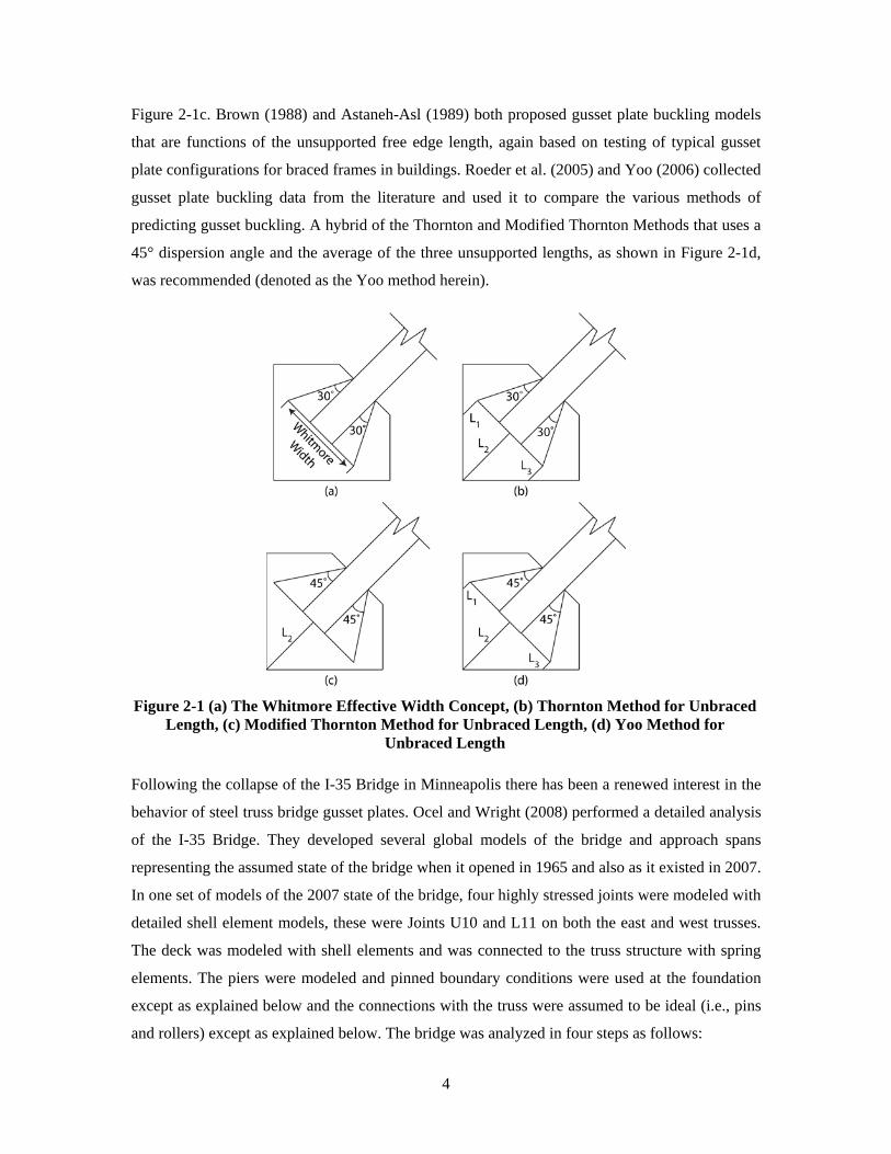
dispersion angle is assumed to calculate the Whitmore effective width as shown in Figure 2-1a.
The connection length in the longitudinal direction of the member is taken as the distance from
the first connector (e.g. bolt, rivet, or initiation of weld) to the end of the connection or last
connector. The predicted maximum uniaxial stress is the member axial load divided by the
Whitmore width times the gusset plate thickness. In his experiments, Whitmore demonstrated that
this assumption provided a conservative estimate of the maximum uniaxial gusset plate stresses at
the ends of members. Bjorhovde and Chakrabarti (1985) demonstrated that the Whitmore width
concept was valid for gusset plates in braced frames and also demonstrated the method was
appropriate for predicting net section fracture. Hardash and Bjorhovde (1985) studied braced
frame gusset plate connections in tension and developed a block shear model based on a
combination of shear and tension net section fracture. Other recent studies such as Yam and
Chang (2002), Sheng et al (2002), and Yoo et al. (2008) have investigated the seismic
performance of gusset plate connections in braced frames under inelastic tension, compression,
and/or cyclic loading.
Several models for estimating the buckling strength of gusset plates have been proposed.
Thornton (1984) suggested the use of the Whitmore width and an unbraced gusset plate length
that is the average of the three lengths, as shown in Figure 2-1b, for use in standard buckling
equations. Yam (1994) developed the Modified Thornton Method for estimating the buckling
capacity, which accounts for load redistribution caused by yielding in the gusset plates prior to
stability failure. The Modified Thornton Method uses a stress dispersion angle of 45° and an
unbraced length in the longitudinal direction of the brace that extends from the centroid of the
brace at the last row of fasteners to the first intersection with gusset plate support as shown in
4
Figure 2-1c. Brown (1988) and Astaneh-Asl (1989) both proposed gusset plate buckling models
that are functions of the unsupported free edge length, again based on testing of typical gusset
plate configurations for braced frames in buildings. Roeder et al. (2005) and Yoo (2006) collected
gusset plate buckling data from the literature and used it to compare the various methods of
predicting gusset buckling. A hybrid of the Thornton and Modified Thornton Methods that uses a
45° dispersion angle and the average of the three unsupported lengths, as shown in Figure 2-1d,
was recommended (denoted as the Yoo method herein).
Following the collapse of the I-35 Bridge in Minneapolis there has been a renewed interest in the
behavior of steel truss bridge gusset plates. Ocel and Wright (2008) performed a detailed analysis
of the I-35 Bridge. They developed several global models of the bridge and approach spans
representing the assumed state of the bridge when it opened in 1965 and also as it existed in 2007.
In one set of models of the 2007 state of the bridge, four highly stressed joints were modeled with
detailed shell element models, these were Joints U10 and L11 on both the east and west trusses.
The deck was modeled with shell elements and was connected to the truss structure with spring
elements. The piers were modeled and pinned boundary conditions were used at the foundation
except as explained below and the connections with the truss were assumed to be ideal (i.e., pins
and rollers) except as explained below. The bridge was analyzed in four steps as follows:
Figure 2-1 (a) The Whitmore Effective Width Concept, (b) Thornton Method for Unbraced
Length, (c) Modified Thornton Method for Unbraced Length, (d) Yoo Method for Unbraced Length
5
• Step 1 simulated construction loading with the deck elements deactivated and the weight
of wet concrete added. Only dead loads were applied and point loads at the end of the
truss were used to simulate the loads from the approach spans.
• Step 2 simulated the bridge just after construction where the weight of the wet concrete
was removed and the deck elements were reactivated (with the deck’s self-weight
included in the elements). Additional loading was added to simulate the weight of
concrete barriers.
• Step 3 simulated the bridge after modifications were made to the concrete barriers and
additional weight was added to the deck to account for the additional deck thickness
added over the years.
• Step 4 simulated the loads believed to be on the bridge at the time of collapse based on
NTSB 07-115 (NTSB 2008). The bridge’s boundary conditions were also modified at this
stage. The bearings were fixed to the piers to simulate conditions observed during
previous live load monitoring of the bridge.
The analyses of the bridge and gusset plate connections indicated that the gusset had significant
yielding under the Step 2 dead loads. The yielding increased as additional load was added to the
bridge and by Step 4 a large percentage of the gusset plate at Joint U10 was yielded. Failure of
the bridge was simulated when the increased stress and deformation due to initial imperfections
for Joint U10 were added. Photos of Joint U10 from prior to the collapse indicated that a vertical
free edge of the gusset was bulged to a magnitude of between 12.7 mm (0.5 in.) to 25.4 mm (1
in.). With an in initial imperfection of 19.1 mm (0.75 in.) the gusset plate at U10 buckled under
the compression diagonal and the bridge suffered a global instability.
Several other issues were investigated such as thermal movements of the bridge, corrosion at
Joint L11, and the effect of deck stiffness. Simulation of the corrosion at Joint 11 was done by
modifying the thickness of elements in the area where corrosion was noted. However, the
simulation did not change the predicted failure mode of the bridge. Neither thermal movements
nor changes in deck stiffness for cracking were found to significantly impact the stress
distribution in the gusset plates. Based on these simulations, the Ocel and Wright (2008)
concluded that buckling of the gusset plate of Joint U10 was a likely cause of the collapse.
Notably, all observed buckling occurred after significant yielding of the gusset.
Higgins et al. (2010) compared block shear and Whitmore section methods for load rating
existing steel truss bridges. The research highlights the fact that vintage steel bridge gusset plates

6
were designed using allowable stress design and Whitmore section approaches but will be load
rated using load and resistance factored rating at strength levels using both Whitmore section
approaches and block shear. Differences in the outcomes of rating the gussets at the allowable
stress and maximum strength levels are identified and simplifications for rating are proposed. A
set of equations for expected LRFR ratings were developed using random sampling and statistical
analysis of several bridges. A method for determining a gusset plate connection design error was
proposed by comparing the actual rating factor to the expected rating factor from the statistically
based equations. The researchers concluded that many bridges designed using Whitmore section
methods will produce rating factors less than 1.0. Two example applications of the proposed
procedure were provided. Notably, other limit states recommended for load rating by FHWA as
described below were not included in the proposed rating factor equations.
2.2 FHWA Load Rating Guidance
The resistance equations in the FHWA Guide are intended to provide for collapse prevention and
are required to be checked for only strength load combinations for Load and Resistance Factor
Rating (LRFR) or for maximum loads in Load Factor Rating (LFR). The FHWA Guide states that
owners may require that connections be evaluated at other loads levels to minimize serviceability
concerns.
Gusset plate strength in tension is governed by the limit states of gross section yield, net section
fracture and block shear. The gross or net areas for gusset plates in tension are calculated using
the Whitmore method (Figure 2-1a), which assumes a 30° dispersion angle for tension stresses as
they are delivered from the tension member to the gusset plate. The block shear strength of the
member connections to the gusset plate is evaluated using a standard block shear check that
considers combined tension yielding and shear fracture or tension fracture and yielding.
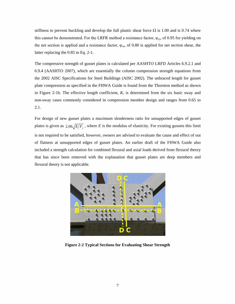
Gusset plate shear strength is evaluated by considering uniform shear stress distributions across
several possible sections as illustrated in Figure 2-2. For LFR, checks of both shear yield on the
gross sections (Lines A-A and C-C in Fig. 2) and shear fracture on net sections (Lines B-B and
D-D) are required using:
( )0.58 0.85 0.58r y g r y nR F A and R F A= Ω = (2-1)
where Ag is gross area along a shear section, An is the net area along a shear section, and Ω is a
reduction factor for the potential of shear buckling along a section. For gusset plates with ample
7
stiffness to prevent buckling and develop the full plastic shear force Ω is 1.00 and is 0.74 where
this cannot be demonstrated. For the LRFR method a resistance factor, φvy, of 0.95 for yielding on
the net section is applied and a resistance factor, φvu, of 0.80 is applied for net section shear, the
latter replacing the 0.85 in Eq. 2-1.
The compressive strength of gusset plates is calculated per AASHTO LRFD Articles 6.9.2.1 and
6.9.4 (AASHTO 2007), which are essentially the column compression strength equations from
the 2002 AISC Specifications for Steel Buildings (AISC 2002). The unbraced length for gusset
plate compression as specified in the FHWA Guide is found from the Thornton method as shown
in Figure 2-1b. The effective length coefficient, K, is determined from the six basic sway and
non-sway cases commonly considered in compression member design and ranges from 0.65 to
2.1.
For design of new gusset plates a maximum slenderness ratio for unsupported edges of gusset
plates is given as 2.06 yE F , where E is the modulus of elasticity. For existing gussets this limit
is not required to be satisfied, however, owners are advised to evaluate the cause and effect of out
of flatness at unsupported edges of gusset plates. An earlier draft of the FHWA Guide also
included a strength calculation for combined flexural and axial loads derived from flexural theory
that has since been removed with the explanation that gusset plates are deep members and
flexural theory is not applicable.
Figure 2-2 Typical Sections for Evaluating Shear Strength
8
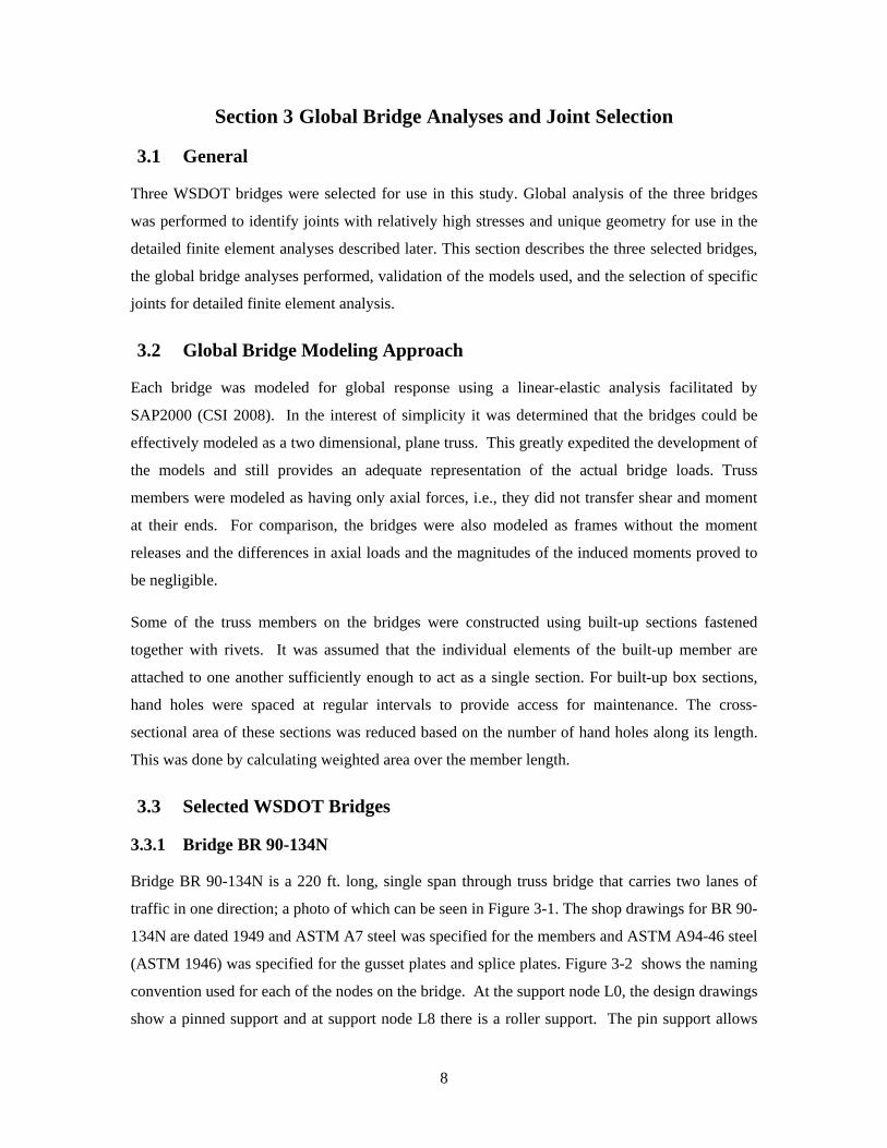
Section 3 Global Bridge Analyses and Joint Selection
3.1 General
Three WSDOT bridges were selected for use in this study. Global analysis of the three bridges
was performed to identify joints with relatively high stresses and unique geometry for use in the
detailed finite element analyses described later. This section describes the three selected bridges,
the global bridge analyses performed, validation of the models used, and the selection of specific
joints for detailed finite element analysis.
3.2 Global Bridge Modeling Approach
Each bridge was modeled for global response using a linear-elastic analysis facilitated by
SAP2000 (CSI 2008). In the interest of simplicity it was determined that the bridges could be
effectively modeled as a two dimensional, plane truss. This greatly expedited the development of
the models and still provides an adequate representation of the actual bridge loads. Truss
members were modeled as having only axial forces, i.e., they did not transfer shear and moment
at their ends. For comparison, the bridges were also modeled as frames without the moment
releases and the differences in axial loads and the magnitudes of the induced moments proved to
be negligible.
Some of the truss members on the bridges were constructed using built-up sections fastened
together with rivets. It was assumed that the individual elements of the built-up member are
attached to one another sufficiently enough to act as a single section. For built-up box sections,
hand holes were spaced at regular intervals to provide access for maintenance. The cross-
sectional area of these sections was reduced based on the number of hand holes along its length.
This was done by calculating weighted area over the member length.
3.3 Selected WSDOT Bridges
3.3.1 Bridge BR 90-134N
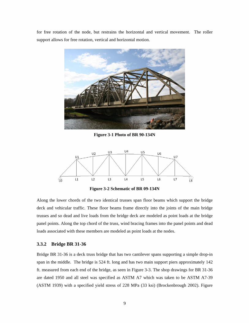
Bridge BR 90-134N is a 220 ft. long, single span through truss bridge that carries two lanes of
traffic in one direction; a photo of which can be seen in Figure 3-1. The shop drawings for BR 90-
134N are dated 1949 and ASTM A7 steel was specified for the members and ASTM A94-46 steel
(ASTM 1946) was specified for the gusset plates and splice plates. Figure 3-2 shows the naming
convention used for each of the nodes on the bridge. At the support node L0, the design drawings
show a pinned support and at support node L8 there is a roller support. The pin support allows
9
for free rotation of the node, but restrains the horizontal and vertical movement. The roller
support allows for free rotation, vertical and horizontal motion.
Along the lower chords of the two identical trusses span floor beams which support the bridge
deck and vehicular traffic. These floor beams frame directly into the joints of the main bridge
trusses and so dead and live loads from the bridge deck are modeled as point loads at the bridge
panel points. Along the top chord of the truss, wind bracing frames into the panel points and dead
loads associated with these members are modeled as point loads at the nodes.
3.3.2 Bridge BR 31-36
Bridge BR 31-36 is a deck truss bridge that has two cantilever spans supporting a simple drop-in
span in the middle. The bridge is 524 ft. long and has two main support piers approximately 142
ft. measured from each end of the bridge, as seen in Figure 3-3. The shop drawings for BR 31-36
are dated 1950 and all steel was specified as ASTM A7 which was taken to be ASTM A7-39
(ASTM 1939) with a specified yield stress of 228 MPa (33 ksi) (Brockenbrough 2002). Figure
Figure 3-2 Schematic of BR 09-134N
Figure 3-1 Photo of BR 90-134N
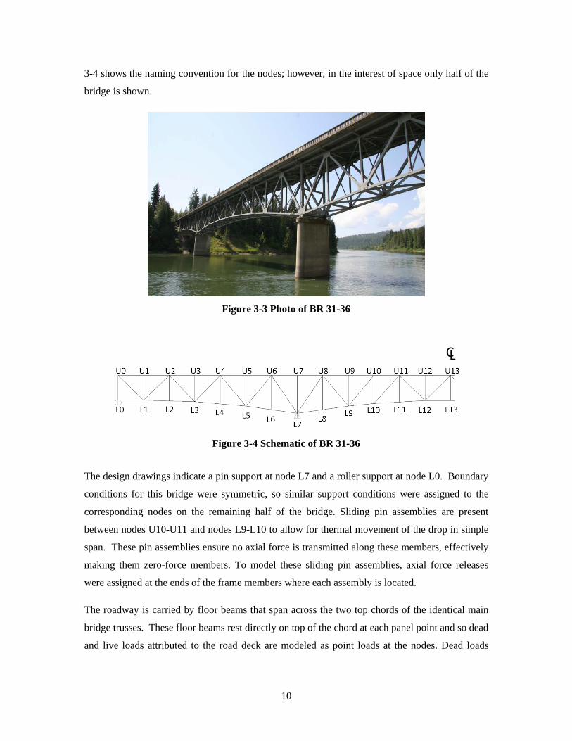
10
3-4 shows the naming convention for the nodes; however, in the interest of space only half of the
bridge is shown.
The design drawings indicate a pin support at node L7 and a roller support at node L0. Boundary
conditions for this bridge were symmetric, so similar support conditions were assigned to the
corresponding nodes on the remaining half of the bridge. Sliding pin assemblies are present
between nodes U10-U11 and nodes L9-L10 to allow for thermal movement of the drop in simple
span. These pin assemblies ensure no axial force is transmitted along these members, effectively
making them zero-force members. To model these sliding pin assemblies, axial force releases
were assigned at the ends of the frame members where each assembly is located.
The roadway is carried by floor beams that span across the two top chords of the identical main
bridge trusses. These floor beams rest directly on top of the chord at each panel point and so dead
and live loads attributed to the road deck are modeled as point loads at the nodes. Dead loads
Figure 3-4 Schematic of BR 31-36
CL
Figure 3-3 Photo of BR 31-36
11
associated with wind bracing and other structural elements that act along the bottom chord are
also modeled as point loads at their corresponding nodes.
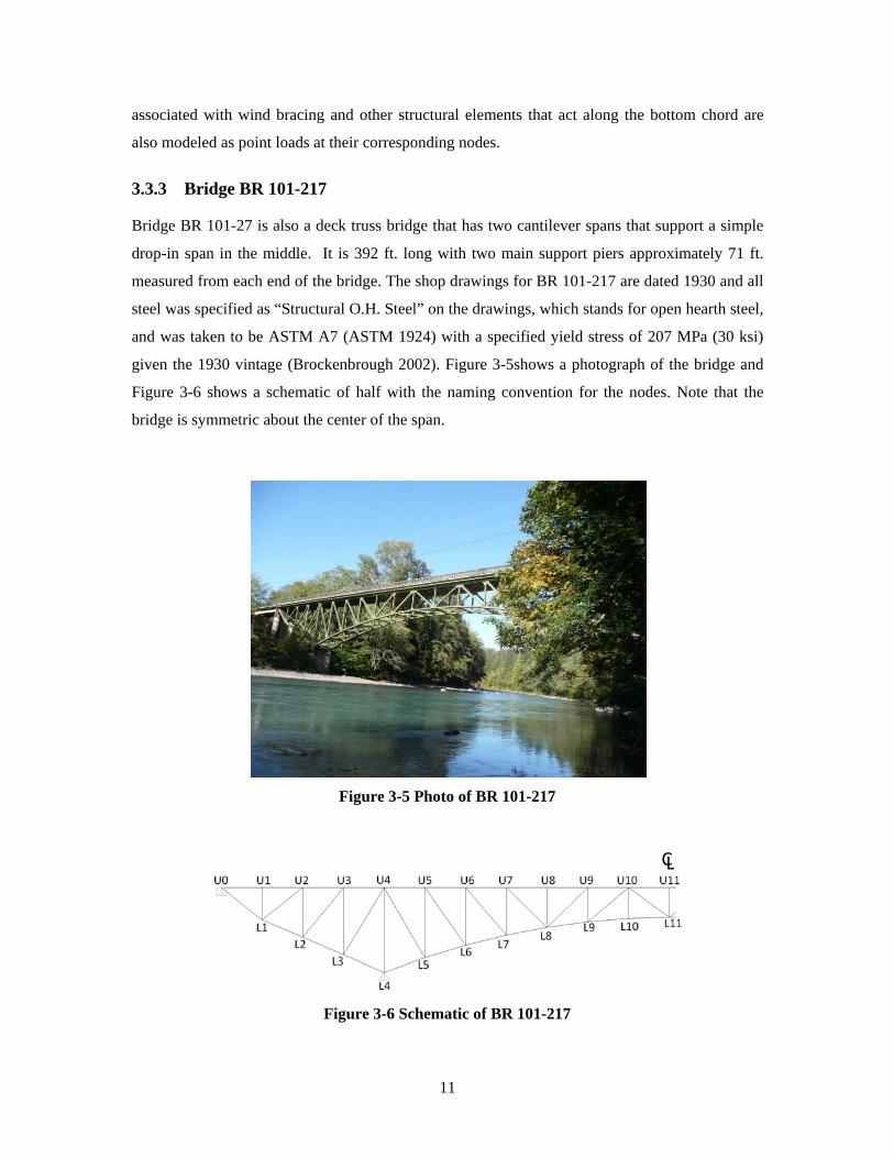
3.3.3 Bridge BR 101-217
Bridge BR 101-27 is also a deck truss bridge that has two cantilever spans that support a simple
drop-in span in the middle. It is 392 ft. long with two main support piers approximately 71 ft.
measured from each end of the bridge. The shop drawings for BR 101-217 are dated 1930 and all
steel was specified as “Structural O.H. Steel” on the drawings, which stands for open hearth steel,
and was taken to be ASTM A7 (ASTM 1924) with a specified yield stress of 207 MPa (30 ksi)
given the 1930 vintage (Brockenbrough 2002). Figure 3-5shows a photograph of the bridge and
Figure 3-6 shows a schematic of half with the naming convention for the nodes. Note that the
bridge is symmetric about the center of the span.
Figure 3-6 Schematic of BR 101-217
CL
Figure 3-5 Photo of BR 101-217
12
A pin support was assigned to node L4 and a roller support was assigned to node U0 consistent
with the drawings. Boundary conditions were symmetric, so similar support types were assigned
to the support nodes for the other half of the bridge. Similar to BR 31-36, BR 104-217 has a drop-
in simple span that requires the need for an expansion joint. This joint is accommodated by
sliding pin assemblies, as described above. These assemblies are located on the members
spanning between nodes L8-L9 and U9-U10. Loads from the road deck are transferred from floor
beams spanning between the main trusses to the panel points along the top chord and are modeled
as point loads at the bridge nodes. Dead loads along the bottom chord attributed to wind bracing
or other structural members are also modeled as point loads at the nodes.
3.4 Bridge and Joint Loads
3.4.1 Bridge Dead and Live Loads
Design drawings for the bridges were carefully examined to determine the appropriate dead loads
for the global bridge models. As noted above, the road deck on all three bridges in question is
carried by floor beams spanning transverse to the main bridge trusses. Loads from the road deck
are distributed to the floor beams based on their tributary areas and then the reactions from the
floor beams are transferred as point loads to the truss nodes. Dead loads from the wind bracing
and other structural elements were also distributed to their appropriate nodes. Unit weights for the
structural steel and concrete used in the dead load determination were 490 and 150 ,
respectively. In addition to the road deck shown in the design drawings, WSDOT recommended
adding a 1.5 in. thick layer of latex modified concrete as a wearing surface. This was applied to
BR 90-134N and BR 31-36 only.
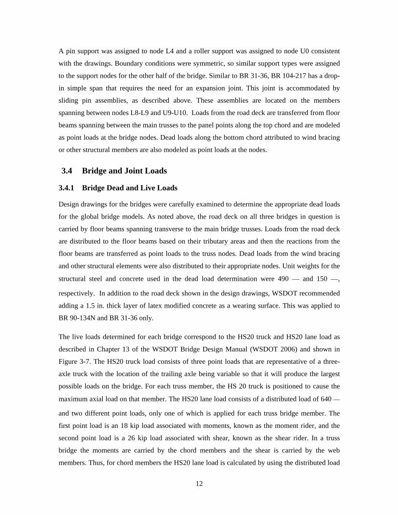
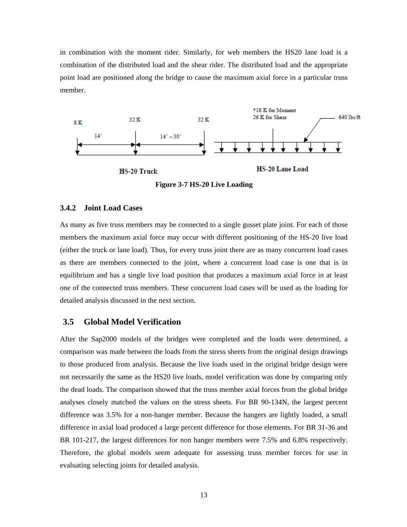
The live loads determined for each bridge correspond to the HS20 truck and HS20 lane load as
described in Chapter 13 of the WSDOT Bridge Design Manual (WSDOT 2006) and shown in
Figure 3-7. The HS20 truck load consists of three point loads that are representative of a three-
axle truck with the location of the trailing axle being variable so that it will produce the largest
possible loads on the bridge. For each truss member, the HS 20 truck is positioned to cause the
maximum axial load on that member. The HS20 lane load consists of a distributed load of 640
and two different point loads, only one of which is applied for each truss bridge member. The
first point load is an 18 kip load associated with moments, known as the moment rider, and the
second point load is a 26 kip load associated with shear, known as the shear rider. In a truss
bridge the moments are carried by the chord members and the shear is carried by the web
members. Thus, for chord members the HS20 lane load is calculated by using the distributed load
13
in combination with the moment rider. Similarly, for web members the HS20 lane load is a
combination of the distributed load and the shear rider. The distributed load and the appropriate
point load are positioned along the bridge to cause the maximum axial force in a particular truss
member.
3.4.2 Joint Load Cases
As many as five truss members may be connected to a single gusset plate joint. For each of those
members the maximum axial force may occur with different positioning of the HS-20 live load
(either the truck or lane load). Thus, for every truss joint there are as many concurrent load cases
as there are members connected to the joint, where a concurrent load case is one that is in
equilibrium and has a single live load position that produces a maximum axial force in at least
one of the connected truss members. These concurrent load cases will be used as the loading for
detailed analysis discussed in the next section.
3.5 Global Model Verification
After the Sap2000 models of the bridges were completed and the loads were determined, a
comparison was made between the loads from the stress sheets from the original design drawings
to those produced from analysis. Because the live loads used in the original bridge design were
not necessarily the same as the HS20 live loads, model verification was done by comparing only
the dead loads. The comparison showed that the truss member axial forces from the global bridge
analyses closely matched the values on the stress sheets. For BR 90-134N, the largest percent
difference was 3.5% for a non-hanger member. Because the hangers are lightly loaded, a small
difference in axial load produced a large percent difference for those elements. For BR 31-36 and
BR 101-217, the largest differences for non hanger members were 7.5% and 6.8% respectively.
Therefore, the global models seem adequate for assessing truss member forces for use in
evaluating selecting joints for detailed analysis.
Figure 3-7 HS-20 Live Loading

14
3.6 Joint Selection
One joint from each bridge was selected for detailed finite element analysis. The selected joints
had a combination of unique geometry and relatively large Whitmore section stresses associated
with at least one member. Each selected joint is described in detail below and the Whitmore
section stresses discussed are for factored loads at the Strength I Load Combination per AASHTO
(2007).
Joint L2 from BR 90-134N was selected for detailed analysis as it had the largest Whitmore
section stress of any joint on the bridge of 131.6 MPa (19.1 ksi) at the end of member L2-L4. As
shown in Figure 3-8 the joint has two 13 mm (1/2 in.) thick gusset plates located on the outer
faces of the members that were specified as silicon steel and taken to be ASTM A94-46 steel
(ASTM 1946), for which a specified yield stress of 310 MPa (45 ksi) was assumed. Both tension
and compression diagonals (L2-U3 and L2-U1 respectively) are built-up box sections as are the
tension chords (L0-L1 and L2-L3), and the hanger is a built-up I-shape. The gusset also serves as
a chord splice, where the splice is offset from the midpoint of the gusset, with the connection for
Chord L2-L4 being longer. A floor beam is attached through a riveted web angle connection and
there is a 9.5 mm (3/8 in.) thick silicon steel gusset plate at the bottom flange of the chords for
attachment of wind bracing that also acts as part of the splice between the tension chords. An
additional 9.5 mm (3/8 in.) thick silicon steel splice plate connects the top flanges of the chords.
Joint L9 from BR 31-36 was also selected for detailed analysis as it had a relatively large stress of
95.8 MPa (13.9 ksi) at the Whitmore section of member L7-L9 and a unique geometry as shown
below. Joint L9 has two 13 mm (1/2 in.) thick gusset plates that are riveted to the outer faces of
the truss members. This connection is at a hinge location in the truss and has a zero force chord
Figure 3-8 Joint L2 from BR 90-134N

15
member attached (L9-L10) with a large pin along where secondary plates increase the bearing
strength of the pin hole for construction loads. The loaded chord is a compression member (L7-
L9) and has a built-up box cross-section composed of channels with riveted top and bottom
plates. There are 13 mm thick (1/2 in.) splice plates on both sides of Chord L7-L9 that help
connect it to the gusset plates. The compression diagonal (L9-U10) is also a built-up box section,
the tension diagonal (L9-U8) is a built-up I-shape of angles and plate, and the vertical hanger is a
rolled W12x53. Wind bracing is connected via a gusset plate attached to the bottom flange of the
loaded chord member and via angles that are riveted to the gusset plates. All steel for this bridge
was specified as A7 with a specified yield stress of 228 MPa (33 ksi).
Joint L5 from BR 101-217 was selected for detailed analysis as it had somewhat large stresses at
the Whitmore Section of the chords but also very different geometry as shown in Figure 3-10. As
shown, L5 is a lower chord connection with a single I-shaped tension diagonal (L5-U4), I-shaped
compression vertical (L5-U5), and built-up compression chords that are composed of channel
sections (L4-L5 and L5-L6) back-to-back at a distance of approximately 280 mm (11 in.). The
chord channels are stitched together with lacing away from gusset plates and solid end plates
adjacent to the gusset connections. The 9.5 mm (3/8 in.) thick gusset plates are positioned
between the back-to-back channels and the diagonal and vertical members pass between the
gusset plates with the vertical member extending through to the bottom flange of the chord, which
is the distinguishing feature for this joint. All truss members are riveted to the gusset, and
therefore the compression diagonal is also riveted to the chords. Wind bracing is present at this
location with transverse gusset plates attached to the top and bottom flanges of the inner channel
of the chord. The chord is spliced at the midpoint of gusset and additional splice plates are present
on the outer webs of the channels. Drawings indicate that the chord members were milled-to-bear
Figure 3-9 Joint L9 from BR 31-36
16
on each other. The steel is specified as “Structural O.H. Steel”, which was assumed to have a
specified yield stress of 207 MPa (30 ksi) as described above.
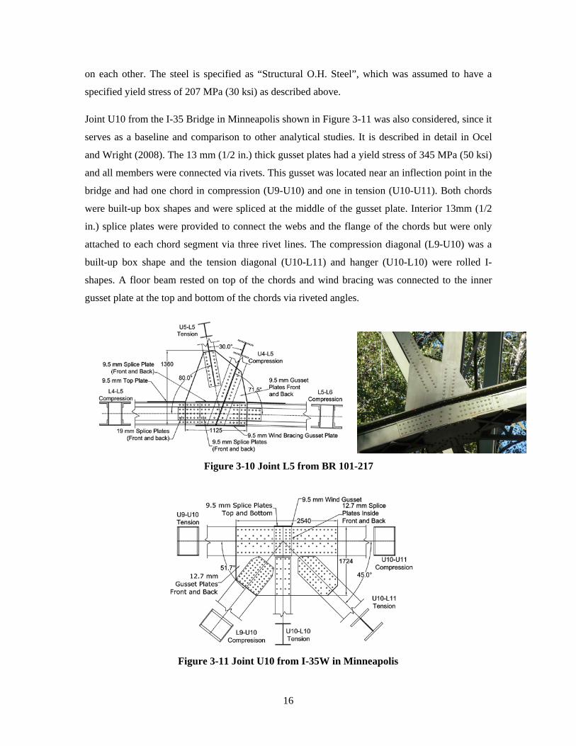
Joint U10 from the I-35 Bridge in Minneapolis shown in Figure 3-11 was also considered, since it
serves as a baseline and comparison to other analytical studies. It is described in detail in Ocel
and Wright (2008). The 13 mm (1/2 in.) thick gusset plates had a yield stress of 345 MPa (50 ksi)
and all members were connected via rivets. This gusset was located near an inflection point in the
bridge and had one chord in compression (U9-U10) and one in tension (U10-U11). Both chords
were built-up box shapes and were spliced at the middle of the gusset plate. Interior 13mm (1/2
in.) splice plates were provided to connect the webs and the flange of the chords but were only
attached to each chord segment via three rivet lines. The compression diagonal (L9-U10) was a
built-up box shape and the tension diagonal (U10-L11) and hanger (U10-L10) were rolled I-
shapes. A floor beam rested on top of the chords and wind bracing was connected to the inner
gusset plate at the top and bottom of the chords via riveted angles.
Figure 3-11 Joint U10 from I-35W in Minneapolis
Figure 3-10 Joint L5 from BR 101-217
17
Section 4 Finite Element Model Development, Validation and Implementation
4.1 Finite Element Model Development
This research uses detailed nonlinear finite element (FE) analysis of detailed models of selected
gusset plates from steel truss bridges to help develop a simplified triage evaluation procedure
(TEP) and compare it with the procedures in the FHWA Guide. As such, the development of a
model of the complex gusset plate connection is necessary and the resulting models must be
validated, despite the lack of experimental data. Detailed FE models of several truss bridge joints
were developed using the ANSYS software package (ANSYS 2008). The development of the
modeling method and verification of the method were done using Joint U10 of the I-35 Bridge
and the computed results from Ocel and Wright (2008). Additional verification is provided by
comparing similarly derived numerical models with prior experimental results. The modeling
methods were then applied to the other joints described below.
The first step in developing the detailed models of the selected joints was to generate CAD
drawings of each joint geometry. To do this, old and sometimes barely legible drawings of the
bridge and bridge joints were used. Where dimensions were unclear or incomplete, assumptions
were made with care taken to preserve the work point of the joints. The resulting CAD drawings
provided coordinates of key points necessary for the generation of the detailed model geometries
in ANSYS.
Four-noded reduced integration shell elements were used to model the gusset plates, splices, wind
bracing plates and truss members in the vicinity of the gusset plates, as shown in Figure 4-1. At a
distance of twice the member depth, d, from the gusset edge the truss members were transitioned
to line elements. This distance was found to adequately model the flow of stress from the member
to the gusset plates when compared with longer distances. A plane-sections-remain-plane master-
slave constraint was applied at this transition. The line elements where assigned the cross-
sectional properties of the truss members and ended at adjacent panel points where all degrees of
freedom except translation in the member’s axial direction were restrained. Thus, the restraint
against gusset buckling provided by the truss members was modeled using the actual truss
member cross-section and length despite the transition from shell elements to line elements.
Loads were applied in the axial direction of the members at these adjacent panel points. Restraint
against out-of-plane displacement of the gusset was provided at the locations where wind bracing
and/or floor beams connected to the gusset.

18
Other methods for applying the boundary conditions and loads were considered. These included
applying loads and boundary conditions at a distance of 2d from the edges of the gusset plates
and not including the beam element transitions. However, that approach was found to result in an
unrealistic restraint of the gusset plate against out-of-plane movement and larger and possibly
unconservative buckling loads. The selected approach more accurately simulated the boundary
conditions for gusset plate buckling; however, the compressive load that can applied to the gusset
is limited by the buckling capacity of the attached beam elements as would be expected in the
bridge.
All rivets were modeled as rigid fasteners. Translational degrees of freedom of nodes at rivet
locations were constrained to be equal for members and gussets plates. Contact or gap elements
were not used at the surfaces, since their use greatly increases the computational time cost and
complexity of analysis without significantly improving the accuracy of the prediction. This leads
to conservative estimates of the gusset plate buckling load, since contact between plates and
members provides additional buckling restraint which is not included with the rigid fastener
method. All gusset plate and splice plate steel was modeled as bilinear kinematic hardening
materials that had an initial elastic modulus of 200 GPa (29,000 ksi) and 3% strain hardening.
The strain hardening was found by linearizing the stress-strain results from material tests from the
I-35 Bridge gusset plate reported in Ocel and Wright (2008). All shell and beam elements
modeling truss members were modeled as elastic elements so that the nonlinear response was
focused upon the gusset plate response.
Figure 4-1 General Gusset Plate Connection Model
19
A mesh refinement study was conducted to determine the mesh density needed to accurately
simulate the general stress field in the gusset plate. Figure 4-2 shows three mesh refinements
considered, having average edge lengths of 38.1 mm (1.5 in.), 25.4 mm (1 in.) and 12.7 mm
(0.5in). The Von Mises stress distributions predicted for these 3 models at the same load levels
are shown in Figure 4-3. The figure shows that the overall stress distributions and magnitudes are
similar for the 25.4 mm and 12.7 mm mesh densities while the 38.1 mm mesh appears to produce
stress distributions that have more sharp changes. The consistency between the 25.4 mm and 12.7
mm mesh densities indicates that there is not a significant increase in accuracy for the finer mesh
while the computational time was increased substantially. Therefore, 25.4 mm average element
size was selected as the target for meshing the U10 gusset plate model from the I-35 Bridge as
well as the other gusset plates considered. Figure 4-4 shows the resulting shell element models for
the three WSDOT joints.

20
(a) (b)
(c)
Figure 4-2 Mesh Refinements Considered: (a) 38.1 mm (1.5 in.) Average Element Edge Length, (b) 25.4 mm (1 in.) Average Element Edge Length, and (c) 12.7 mm (0.5 in.)
Average Element Edge Length

21
(a) (b)
(c)
Figure 4-3 Von Mises Stress Distributions (ksi) for (a) 38.1 mm (1.5 in.) Average Element Edge Length Mesh, (b) 25.4 mm (1 in.) Average Element Edge Length Mesh, and (c) 12.7
mm (0.5 in.) Average Element Edge Length Mesh

22
4.2 Validation of Finite Element Models
The modeling methods described above were applied to the simulation of gusset plate
connections in braced frames by Yoo et al. (2008). Similarities between those simulations and the
models used here include the software, elements and material constitutive models. Yoo et al.
(2008) demonstrated excellent agreement with experimental results, both in terms of global
response of the braced frame system and with simulating local gusset plate stresses as shown in
Figure 4-5. The figure illustrates that the regions of high stress, signified experimentally by the
flaking of whitewash, match well with the areas of high stress from the simulation. It should be
noted that the gusset plates in the referenced concentrically braced frames were subjected to large
out-of-plane deformations as brace buckling occurred and had inelastic behavior. In the truss
bridge gusset plate models developed here the analyses are kept largely within the elastic range of
(a) (b)
(c)
Figure 4-4 Truss Bridge Joint Models (a) Joint L2 from BR 90-134N, (b) Joint L9 from BR 31-36, and (c) Joint L5 from BR 101-217.

23
behavior and the out-of-plane deformations are expected to be small. Regardless of the
differences between truss bridge and braced frame gusset plates, the results in Figure 4-5 provide
confidence in the ability of shell element models to capture buckling deformations and local
stress distributions.
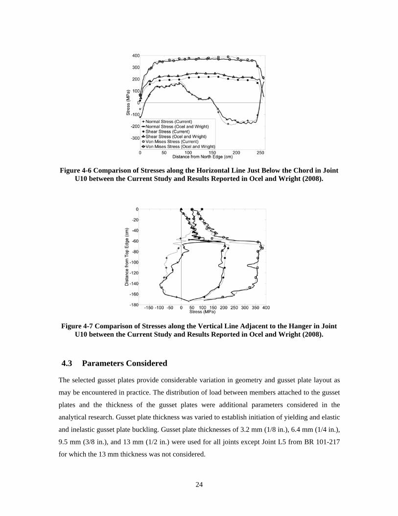
To provide additional verification of the modeling techniques used here, the results of the
analysis of Joint U10 from the I-35 Bridge were compared with analysis results given in Ocel and
Wright (2008). In that study, the entire bridge was modeled in three-dimensions primarily using
beam elements for the steel superstructure and shell elements for the deck with a detailed shell
element mesh to model Joint U10. Thus the actual boundary conditions for the joint were
simulated from the global bridge response. Figures 4-6 and 4-7 compare stress results for the two
models under the approximate loading for the bridge at the time of collapse, as given in Ocel and
Wright. Figure 4-6 compares Von Mises, shear and normal stresses along a horizontal line one
element below the lower rivet line of the chord connection and shows reasonable agreement.
Figure 4-7 compares the same stresses along a vertical line one element away from the hanger
rivet line and again shows reasonable agreement. Therefore, the four gusset plate connections
were simulated with these modeling procedures.
Figure 4-5 Comparison of Gusset Plate Stresses and Whitewash Flaking from Yoo et al.
(2008)
24
4.3 Parameters Considered
The selected gusset plates provide considerable variation in geometry and gusset plate layout as
may be encountered in practice. The distribution of load between members attached to the gusset
plates and the thickness of the gusset plates were additional parameters considered in the
analytical research. Gusset plate thickness was varied to establish initiation of yielding and elastic
and inelastic gusset plate buckling. Gusset plate thicknesses of 3.2 mm (1/8 in.), 6.4 mm (1/4 in.),
9.5 mm (3/8 in.), and 13 mm (1/2 in.) were used for all joints except Joint L5 from BR 101-217
for which the 13 mm thickness was not considered.
Figure 4-7 Comparison of Stresses along the Vertical Line Adjacent to the Hanger in Joint
U10 between the Current Study and Results Reported in Ocel and Wright (2008).
Figure 4-6 Comparison of Stresses along the Horizontal Line Just Below the Chord in Joint
U10 between the Current Study and Results Reported in Ocel and Wright (2008).
25
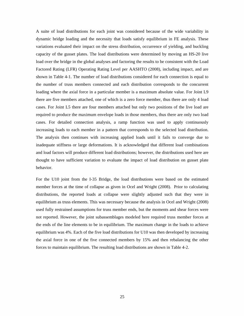
A suite of load distributions for each joint was considered because of the wide variability in
dynamic bridge loading and the necessity that loads satisfy equilibrium in FE analysis. These
variations evaluated their impact on the stress distribution, occurrence of yielding, and buckling
capacity of the gusset plates. The load distributions were determined by moving an HS-20 live
load over the bridge in the global analyses and factoring the results to be consistent with the Load
Factored Rating (LFR) Operating Rating Level per AASHTO (2008), including impact, and are
shown in Table 4-1. The number of load distributions considered for each connection is equal to
the number of truss members connected and each distribution corresponds to the concurrent
loading where the axial force in a particular member is a maximum absolute value. For Joint L9
there are five members attached, one of which is a zero force member, thus there are only 4 load
cases. For Joint L5 there are four members attached but only two positions of the live load are
required to produce the maximum envelope loads in those members, thus there are only two load
cases. For detailed connection analysis, a ramp function was used to apply continuously
increasing loads to each member in a pattern that corresponds to the selected load distribution.
The analysis then continues with increasing applied loads until it fails to converge due to
inadequate stiffness or large deformations. It is acknowledged that different load combinations
and load factors will produce different load distributions; however, the distributions used here are
thought to have sufficient variation to evaluate the impact of load distribution on gusset plate
behavior.
For the U10 joint from the I-35 Bridge, the load distributions were based on the estimated
member forces at the time of collapse as given in Ocel and Wright (2008). Prior to calculating
distributions, the reported loads at collapse were slightly adjusted such that they were in
equilibrium as truss elements. This was necessary because the analysis in Ocel and Wright (2008)
used fully restrained assumptions for truss member ends, but the moments and shear forces were
not reported. However, the joint subassemblages modeled here required truss member forces at
the ends of the line elements to be in equilibrium. The maximum change in the loads to achieve
equilibrium was 4%. Each of the five load distributions for U10 was then developed by increasing
the axial force in one of the five connected members by 15% and then rebalancing the other
forces to maintain equilibrium. The resulting load distributions are shown in Table 4-2.
26
Table 4-1 Member Loads for Different Load Distribution Cases (kN)
Joint L2 (BR 90-134N)
Load Case L1-L2 U1-L2 U2-L2 L2-U3 L2-L3
1 2078 1214 192 -635 3325
2 2006 1464 199 -594 3404
3 2112 1431 205 -562 3465
4 1775 1281 173 -858 3199
5 2040 1359 196 -771 3474
Joint L9 (BR 31-36)
Load Case L8-L9 U8-L9 U9-L9 L9-U10 L9-L10
1 -2576 1994 -372 -1998 0
2 -2404 2033 -604 -1699 0
3 -2298 2005 -669 -1565 0
4 -2480 1931 -373 -1914 0
Joint L5 (BR 101-217)
Load Case L4-L5 U4-L5 U5-L5 L5-L6
1 -3579 931 -1153 -3022
2 -3174 1092 -1293 -2540
Table 4-2 Member Loads for Different Load Distribution Cases for U10 from I-35 (kN)
Load Case U9-U10 L9-U10 L10-U10 U10-L11 U10-U11
1 10585 -11233 2289 9230 -2903
2 10477 -11565 2448 9373 -3318
3 9249 -10501 2522 8089 -2903
4 10205 -10637 1637 9492 -3099
5 8760 -10232 2194 8254 -3417
27
Section 5 Behavior of Truss Bridge Joints, Observations, and Development of the Triage Evaluation Procedure
5.1 Gusset Plate Yielding
5.1.1 Observed Behavior
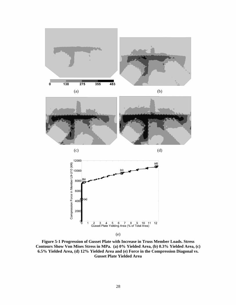
Each joint analysis developed large areas of gusset plate yielding, identified as the regions where
the Von Mises stress exceeds the yield stress of the gusset plate, prior to convergence failure of
the analysis. An example of the progression of gusset plate yielding with increasing truss member
loads is shown in Figure 5-1 for Joint U10 from the I-35 Bridge, where the contours depict the
Von Mises stress and the black areas are those that have yielded. As shown, yielding begins
approximately 250 mm from the end of the compression diagonal. With increasing load the
yielding spreads horizontally across the gusset plate and around the ends of the diagonals. At the
onset of yielding the calculated maximum Whitmore stress from any truss member was 203 MPa,
59% of the gusset plate yield stress, and as shown, yielding initiates away from the end of the
diagonal. While the maximum uniaxial stress is observed at the end of the connected member, in
agreement with the observation of Whitmore (1952), yielding is controlled by a biaxial stress
state involving the interaction of stresses from the members. This interaction and the
corresponding onset of yielding have been observed from the analyses to occur within a critical
region defined by a triangle bounded by the rivet lines for the chord and hanger, and the end of
the diagonal. Figure 5-1b shows the onset of gusset plate yielding occurring in this location for
Joint U10.
Figure 5-1e shows the percentage of gusset plate area that is yielding relative to the axial load in
the compression diagonal for Joint U10. The figure shows that once yielding begins it spreads
fairly rapidly and that the onset of yielding can be reasonably approximated to correspond to
yielding of 0.5% of the gusset plate area. This represents a small percentage of the total gusset
plate area but a significant portion of the critical area that supports the diagonal, where yielding
can cause instability resulting in inelastic gusset plate buckling. Further, yielding of this extent
under service loads would be undesirable. Figure 5-2 shows 0.5% of the gusset plate area for the
four joints considered in this study to demonstrate the onset of yielding as defined here.
28
(a) (b)
(c) (d)
(e)
Figure 5-1 Progression of Gusset Plate with Increase in Truss Member Loads. Stress Contours Show Von Mises Stress in MPa. (a) 0% Yielded Area, (b) 0.3% Yielded Area, (c) 6.5% Yielded Area, (d) 12% Yielded Area and (e) Force in the Compression Diagonal vs.
Gusset Plate Yielded Area

29
5.1.2 Proposed Triage Evaluation Procedure: Yielding
Yielding will in general occur prior to gusset plate failure modes such as block shear or buckling
because block shear failure requires the development of stresses large enough to cause fracture
and gusset plate buckling has been observed to in general be inelastic buckling. Therefore,
yielding is a reasonable limit state to use for a rapid evaluation procedure. As described above,
yielding in truss bridge gusset plate connections generally initiates in an interference zone as
illustrated in Figure 5-3. Since the onset of yielding has been observed to occur prior to the
Whitmore stress at the ends of the attached members reaching the yield stress it appears that the
interactions of the stresses generated from the connected truss members must be considered.
Figure 5-4 illustrates how the stresses from the two diagonal members connected to a gusset plate
may interfere with each other. Here, a simple method for combining these stresses is developed.
While more complex and accurate methods may be possible and are the focus of future research,
(a) (b)
(c) (d)
Figure 5-2 Illustration of 0.5% of Gusset Plate Area Yielding for (a) Joint L2 of BR 90-134N, (b) Joint L9 of BR 31-36, (c) Joint L5 of BR 101-217 and (d) Joint U10 of I-35

30
the objective of the current endeavor is to develop a conservative, simple and straightforward
process for evaluating gusset plates for the onset of yielding.
The Whitmore method conservatively predicts the maximum uniaxial stresses in the gusset at the
end of a riveted member connection, which are denoted σ11 and σ22 in Figure 5-4. The TEP
conservatively assumes these uniaxial stresses to be principle stresses, denoted σ1 and σ2,
respectively. The most adverse condition occurs when these stresses for different members are
orthogonal to each other and opposite in sign. Applying this assumption to the condition in Figure
5-4 results in θ1 = θ2, the Whitmore uniaxial stresses being principle stresses for the stress block
shown, the shear stress on that stress block being zero, and the shear stress on a stress block
rotated 45° from the diagonals to be the maximum shear stress. As a result, the Von Mises yield
criteria for plane stress will govern yielding of the gusset:
2 2 2
1 1 2 2 yσ σ σ σ σ− + = (3-1)
where σ1 and σ2 are principle stresses and σy is the yield stress. Thus, for the very worst case of σ1
and σ2 being equal magnitude and opposite sign, yielding will occur when . To apply
this notion to gusset plates in bridges it is necessary to determine the maximum Whitmore stress
for all members intersecting the gusset, σw,max, and the proposed yield check in the TEP is:
,max 3w yFσ ≤ (3-2)
where Fy is the yield stress of the gusset plate.
Figure 5-3 Interference of Stresses in Gusset Plate Connections
Yielding observed to
occur here first

31
5.1.3 Comparison with the TEP and FHWA Guide: Yielding
For each analysis that did not exhibit elastic buckling (typically gusset plates above 3.2 mm (1/8
in.) thick) the truss member loads at the point in the analysis where 0.5% of the gusset plate is
yielding was recorded. Those loads were then used to compute the values shown in Table 5-1,
which include the maximum uniaxial stress on the Whitmore section (considering all members),
σw,max, and the maximum gross shear stress (considering multiple shear sections), τmax for the
gusset plates at their actual thicknesses. For Joint L5 no shear stress is shown because both
possible shear lines pass through either a chord or vertical hanger since the chord is continuous
through the gusset and the vertical hanger passes through the gusset to the bottom of the chord as
shown in Figure 3-10. Table 5-1 demonstrates that when the onset of gusset plate yielding occurs
the maximum uniaxial stress on the Whitmore section and maximum shear stress are both below
yield when compared to Fy and 3yF values, respectively, the latter value being an
approximation of the yield stress in shear. Thus, neither the shear stress nor Whitmore stress
evaluations in the FHWA Guide identify the onset of gusset plate yielding. This is not surprising
since the shear stress evaluation methods assume full shear yielding over the entire selected shear
section and yielding along the entire Whitmore width at the end of a truss member implies that
the stresses are uniaxial and are not influenced by stresses generated by other members. However,
Table 5-1 does indicate that the maximum Whitmore stresses at the onset of yield are larger than
or equal to 3yF , which is the proposed limit for the Whitmore stress in the TEP.
Figure 5-4 Interference of Stresses in Gusset Plate Connections
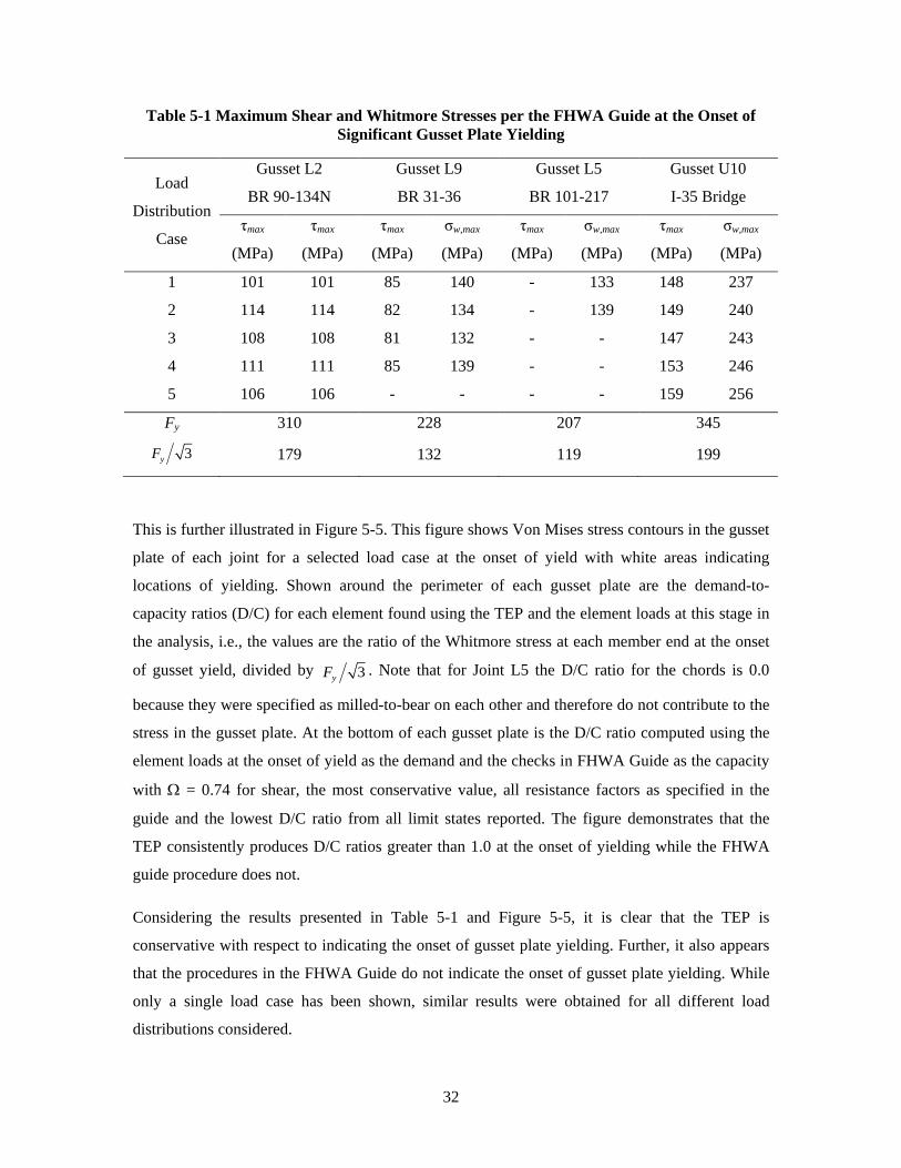
32
Table 5-1 Maximum Shear and Whitmore Stresses per the FHWA Guide at the Onset of Significant Gusset Plate Yielding
Load
Distribution
Case
Gusset L2
BR 90-134N
Gusset L9
BR 31-36
Gusset L5
BR 101-217
Gusset U10
I-35 Bridge
τmax
(MPa)
τmax
(MPa)
τmax
(MPa)
σw,max
(MPa)
τmax
(MPa)
σw,max
(MPa)
τmax
(MPa)
σw,max
(MPa)
1 101 101 85 140 - 133 148 237
2 114 114 82 134 - 139 149 240
3 108 108 81 132 - - 147 243
4 111 111 85 139 - - 153 246
5 106 106 - - - - 159 256
Fy 310 228 207 345
3yF 179 132 119 199
This is further illustrated in Figure 5-5. This figure shows Von Mises stress contours in the gusset
plate of each joint for a selected load case at the onset of yield with white areas indicating
locations of yielding. Shown around the perimeter of each gusset plate are the demand-to-
capacity ratios (D/C) for each element found using the TEP and the element loads at this stage in
the analysis, i.e., the values are the ratio of the Whitmore stress at each member end at the onset
of gusset yield, divided by 3yF . Note that for Joint L5 the D/C ratio for the chords is 0.0
because they were specified as milled-to-bear on each other and therefore do not contribute to the
stress in the gusset plate. At the bottom of each gusset plate is the D/C ratio computed using the
element loads at the onset of yield as the demand and the checks in FHWA Guide as the capacity
with Ω = 0.74 for shear, the most conservative value, all resistance factors as specified in the
guide and the lowest D/C ratio from all limit states reported. The figure demonstrates that the
TEP consistently produces D/C ratios greater than 1.0 at the onset of yielding while the FHWA
guide procedure does not.
Considering the results presented in Table 5-1 and Figure 5-5, it is clear that the TEP is
conservative with respect to indicating the onset of gusset plate yielding. Further, it also appears
that the procedures in the FHWA Guide do not indicate the onset of gusset plate yielding. While
only a single load case has been shown, similar results were obtained for all different load
distributions considered.
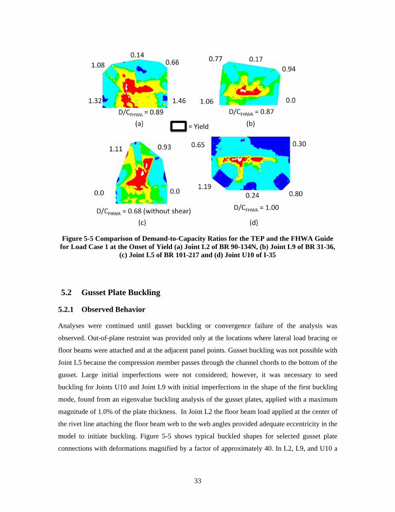
33
5.2 Gusset Plate Buckling
5.2.1 Observed Behavior
Analyses were continued until gusset buckling or convergence failure of the analysis was
observed. Out-of-plane restraint was provided only at the locations where lateral load bracing or
floor beams were attached and at the adjacent panel points. Gusset buckling was not possible with
Joint L5 because the compression member passes through the channel chords to the bottom of the
gusset. Large initial imperfections were not considered; however, it was necessary to seed
buckling for Joints U10 and Joint L9 with initial imperfections in the shape of the first buckling
mode, found from an eigenvalue buckling analysis of the gusset plates, applied with a maximum
magnitude of 1.0% of the plate thickness. In Joint L2 the floor beam load applied at the center of
the rivet line attaching the floor beam web to the web angles provided adequate eccentricity in the
model to initiate buckling. Figure 5-5 shows typical buckled shapes for selected gusset plate
connections with deformations magnified by a factor of approximately 40. In L2, L9, and U10 a
Figure 5-5 Comparison of Demand-to-Capacity Ratios for the TEP and the FHWA Guide for Load Case 1 at the Onset of Yield (a) Joint L2 of BR 90-134N, (b) Joint L9 of BR 31-36,
(c) Joint L5 of BR 101-217 and (d) Joint U10 of I-35

34
sidesway buckling mode was observed with the compression diagonal swaying to one side of the
gusset.
Inelastic gusset plate buckling was common and elastic buckling was observed only with
extremely thin (3.2 mm [1/8 in.]) gusset plates. Where buckling was observed, the out-of-plane
displacements of the gusset plate nodes at locations shown in Figure 5-7a were recorded. Figure
5-7b shows the typical progression of out-of-plane displacement along the line parallel to the
compression member. Similar behavior was observed along the free edge. Since contact between
the gusset plate and truss members was not modeled some of the gusset nodes deform into the
truss members causing a conservative estimate of gusset plate buckling capacity. Compressive
force versus maximum out-of-plane displacement was plotted for both locations of Figure 5-7a
and the buckling load was conservatively taken as the load at the intersection of the initial tangent
and the tangent representing 15% of the initial tangent as demonstrated in Figure 6-6. For all
cases, the buckling load found using the node at the free edge and the buckling load found using
the node aligned with the compression diagonal were within 5%, with the latter typically being
lower and used for the buckling loads reported herein.
(a) (b)
Figure 5-6 Buckled Shapes of (a) Joint L2 of BR 90-134N and (b) Joint U10 of I-35
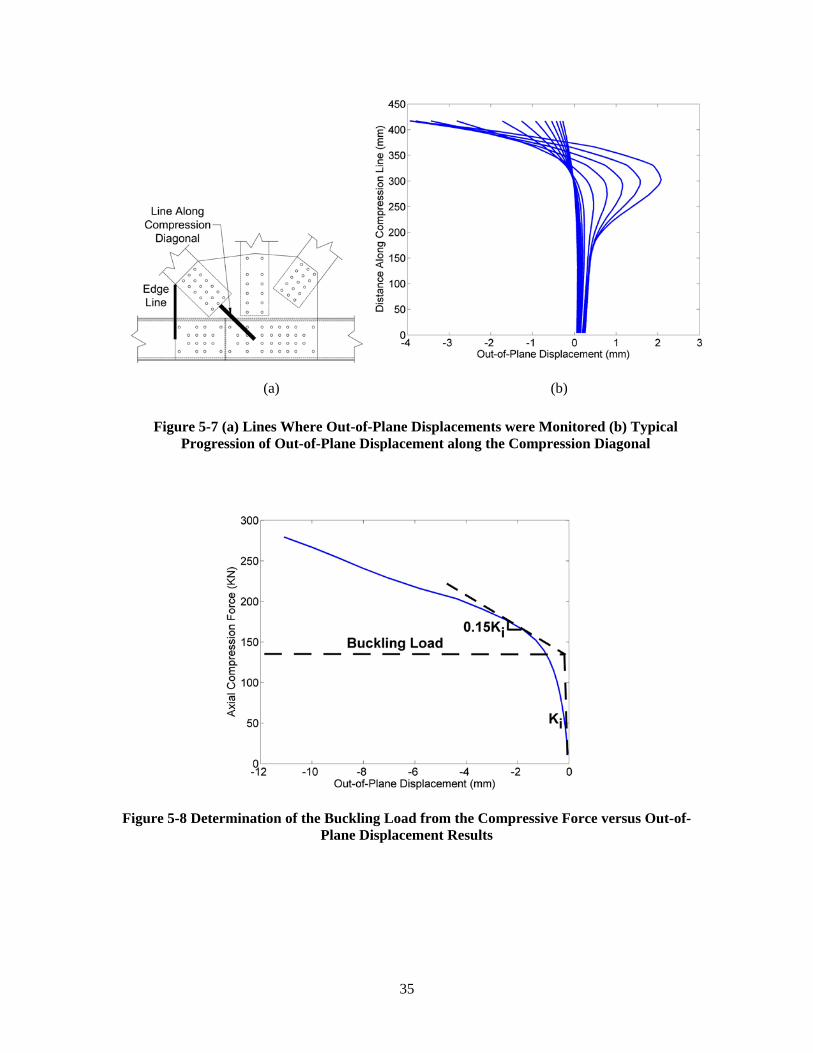
35
Figure 5-8 Determination of the Buckling Load from the Compressive Force versus Out-of-Plane Displacement Results
(a) (b)
Figure 5-7 (a) Lines Where Out-of-Plane Displacements were Monitored (b) Typical Progression of Out-of-Plane Displacement along the Compression Diagonal

36
5.2.2 Comparison with Simplified Calculations for Gusset Plate Buckling Capacity
The three methods shown in Figure 2-1 for calculating the unbraced compression length and
compressive stress for buckling (Thornton, Modified Thornton, and Yoo, respectively) were
considered for use in calculating the gusset plate buckling capacity with the AASHTO column
buckling equations (AASHTO 2007). Figures 5-9a, 5-9b and 5-9c compare the buckling strength
calculated with the three methods with the buckling load established from the analyses for several
different values of the effective length factor, K, and a yield stress of 345 MPa (the maximum
yield stress for any of the gusset plates). All curves and data are shown versus L/t, where L is the
unbraced length per the corresponding method and t is the gusset plate thickness and the observed
buckling stresses have been normalized by the actual gusset plate yield stress. Each figure shows
56 data points, 20 from Joint L2 of BR 90-134N, 20 from Joint U10 of the I-35 Bridge and 16
from Joint L9 of BR 31-36. Variations in both the gusset thickness and in the load distribution
were considered. Cases where global or local buckling of a truss member occurred prior to gusset
plate buckling were excluded from the data and were common when the thicker gusset plates
were used.
As shown in Figures 5-9a and 5-9c, the Thornton and Yoo methods appear unconservative at low
values of L/t for any value of K and both result in two of three unbraced lengths used in the
average unbraced length being zero for all three gusset plate configurations considered. Thus, the
average unbraced length is small even when the gusset thickness is small. However, the Modified
Thornton Method proposed by Yam (1994), which uses only the unbraced length aligned with the
compression diagonal’s centroid, is shown to be reasonably conservative in Figure 5-9b with K of
1.0. Based on these results, the Modified Thornton Method is recommended for calculating the
unbraced length as part of the proposed TEP. Note that the gusset plates considered here
displayed inelastic buckling at their actual thickness and the yield check of the TEP governed
over gusset plate buckling, which is likely to be the case for most gusset plate configurations.
Buckling loads were compared to the necessary to cause the onset of gusset plate yielding. For all
joints on the three WSDOT bridges with gusset plates at their design thicknesses compressive
buckling loads were calculated for the gusset plates attached to the compression diagonal using
the proposed method with a resistance factor, φP, of 0.9. When compared to the values obtained
for checking the onset of gusset plate yielding per the TEP with no resistance factor, it was found
that the buckling load is consistently larger than the force associated with the TEP yield check.

37
5.3 Comparison of Block Shear and the TEP Yield Check
To ensure that the TEP check for the onset of gusset plate is conservative with respect block
shear, a small parametric study was performed using the generalized member-to-gusset plate
connection shown in Figure 5-10. Note that the connection to the gusset plate may be symmetric
in the case of diagonal or hanger attachment or it may not be symmetric in the case of a chord
connection. The variables defining the connection geometries are: Lvg = gross shear length, Lvn =
net shear length, Ltg = gross tension length, Ltn = net tension length, nrt = number of rivets along
the tension line, nrv = number of rivets along the shear line, d = rivets diameter, and tp = gusset
(a) (b)
(c)
Figure 5-9 Comparison of Buckling Stress versus Effective Length from Analysis with Buckling Stress Predicted Using (a) the Thornton Method, (b) the Modified Thornton
Method, and (c) the Yoo Method
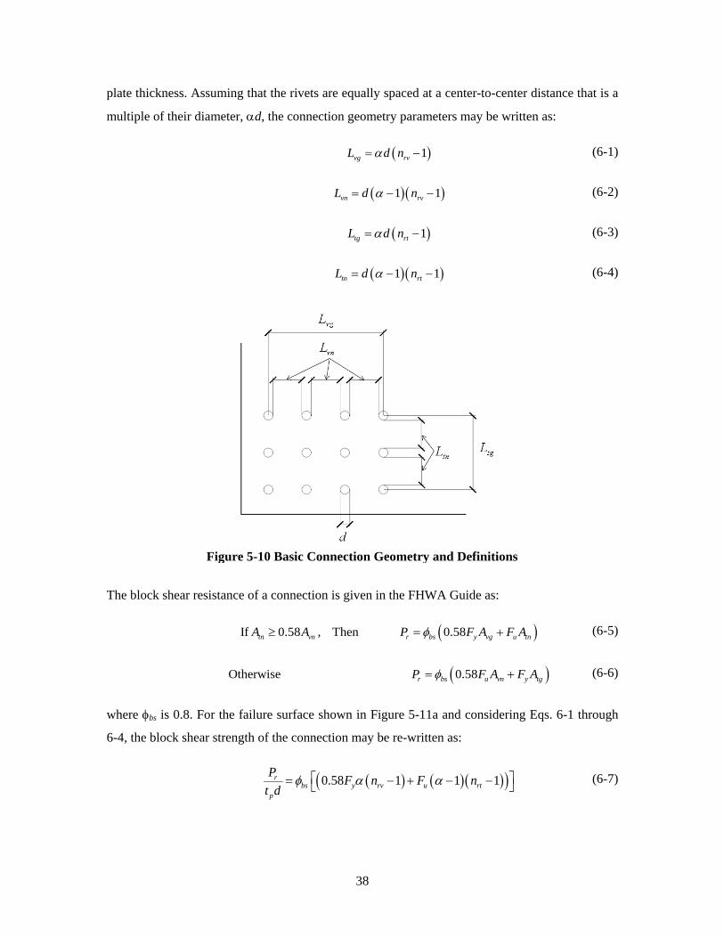
38
plate thickness. Assuming that the rivets are equally spaced at a center-to-center distance that is a
multiple of their diameter, αd, the connection geometry parameters may be written as:
( )1vg rvL d nα= − (6-1)
( )( )1 1vn rvL d nα= − − (6-2)
( )1tg rtL d nα= − (6-3)
( )( )1 1tn rtL d nα= − − (6-4)
The block shear resistance of a connection is given in the FHWA Guide as:
( )If 0.58 , Then 0.58tn vn r bs y vg u tnA A P F A F Aφ≥ = + (6-5)
( )Otherwise 0.58r bs u vn y tgP F A F Aφ= + (6-6)
where φbs is 0.8. For the failure surface shown in Figure 5-11a and considering Eqs. 6-1 through
6-4, the block shear strength of the connection may be re-written as:
( ) ( )( )( )0.58 1 1 1rbs y rv u rt
p
P F n F nt d
φ α α = − + − − (6-7)
Figure 5-10 Basic Connection Geometry and Definitions

39
( )( ) ( )( )0.58 1 1 1rbs U rv u rt
p
P F n F nt d
φ α α = − − + − (6-8)
where the small section indicated in Figure 5-11a have been conservatively negelected. Similarly,
considering the Whitmore section shown in Figure 5-11b, the TEP yield force may be written as:
( ) ( )1 1 30
3rt rv yr
p
n n tan FPt d
α − + − ° = (6-9)
Eqns (6-7), (6-8) and (6-9) are then used to compare the resistance calculated from block shear to
that calculated from the TEP yield check. Figure 5-12 shows the ratio of block shear capacity to
the TEP yield strength for a reasonable range of connection parameters and material strengths.
Note that ASTM specification through 1949 specified that the yield stress, Fy, be ½ the tensile
stress, Fu, for structural steel while also meeting an additional specified lower bound
(Brockenbrough 2002). Thus, the range of the ratio Fu/Fy considered in Figure 5-12 is adequate.
Further, it has been observed from various truss bridge joint drawings that the spacing of the
rivets is not likely to be less than 3d. Therefore, the values of α considered (3 and 4) are
representative of the likely values as well. As Figure 5-12 shows, block shear strength is never
less than the TEP yield strength.
The same process was followed for block shear failure surfaces and Whitmore sections typical of
a diagonal or hanger connection as shown in Figure 5-13. The ratio of block shear strength to
(a) (b)
Figure 5-11 (a) Block Shear Failure Surface for Chord and (b) Whitmore Section for Chord Used for TEP Stress Calculation
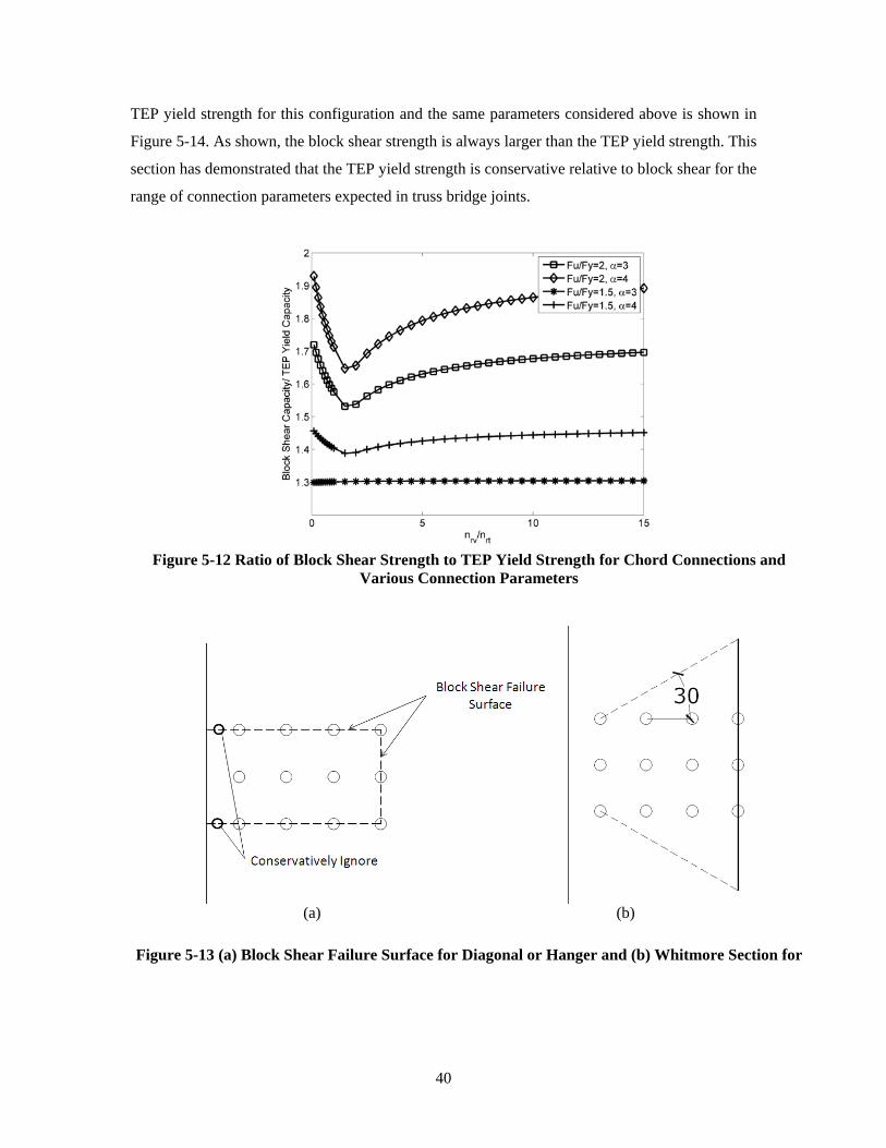
40
TEP yield strength for this configuration and the same parameters considered above is shown in
Figure 5-14. As shown, the block shear strength is always larger than the TEP yield strength. This
section has demonstrated that the TEP yield strength is conservative relative to block shear for the
range of connection parameters expected in truss bridge joints.
(a) (b)
Figure 5-13 (a) Block Shear Failure Surface for Diagonal or Hanger and (b) Whitmore Section for
Figure 5-12 Ratio of Block Shear Strength to TEP Yield Strength for Chord Connections and
Various Connection Parameters
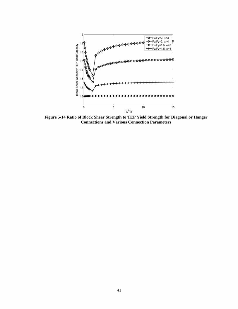
41
Figure 5-14 Ratio of Block Shear Strength to TEP Yield Strength for Diagonal or Hanger
Connections and Various Connection Parameters

42
Section 6 Application of the TEP
6.1 General
As described above, the TEP consists of three primary checks, namely, gusset plate yielding,
gusset plate buckling and fastener strength. Here, the fastener strength is not considered and is
instead discussed in Section 8. Therefore, the following recommended checks are applied to truss
bridge joints as part of the TEP in this section:
1. Gusset plate compression and tension yielding: Compare the maximum Whitmore stress,
using a 30° dispersion angle, from any connected member with 3yF , where Fy is the
yield stress of the gusset.
2. Gusset plate buckling: The buckling equations in the AASHTO LRFD (AASHTO 2007)
are recommended for evaluating gusset plate buckling with an effective length factor, K,
of 1.0. The Modified Thornton Method by Yam (1994) is recommended for establishing
the unbraced length and the gusset section properties, where the unbraced length is taken
as the distance from the end of the compression member connection to the next line of
gusset plate support (typically a gusset-to-chord connection rivet line) and a 45°
dispersion angle is used.
6.2 Joint U10 of I-35W
Prior to applying the TEP to the selected WSDOT bridges it was applied to Joint U10 of I-35W as
this joint should be identified as a problem joint in the TEP as it has been shown to have been
overstressed by this analytical study and others (Ocel and Wright 2008). Three loading conditions
from Ocel and Wright (2008) were considered for Joint U10: (i) the loads denoted Step 2 that are
an estimate of the forces due to the dead loads when the bridge first opened for service, (ii) the
loads denoted Step 3 that are an estimate of the forces due to the dead loads after modifications
were made to the bridge in 1999 and (iii) the estimated loads at the time of collapse. Table 6-1
shows demand-to-capacity ratios (DC ratios) for these three loading conditions for Joint U10,
where the demand is the maximum Whitmore stress considering all members and the capacity is
3yF per the TEP. As shown in Table 6-1 the DC ratio is 1.04 for the Step 2 loading, which
indicates this gusset plate was likely to be yielding under only dead loads when the bridge opened
for service. With the addition of the construction and traffic loads estimated to be on the bridge at
the time of collapse the DC ratio climbs to 1.42 for the TEP. Gusset plate yielding at both load
levels has indeed been confirmed by finite element analyses conducted as part of this research
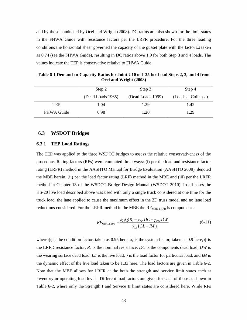
43
and by those conducted by Ocel and Wright (2008). DC ratios are also shown for the limit states
in the FHWA Guide with resistance factors per the LRFR procedure. For the three loading
conditions the horizontal shear governed the capacity of the gusset plate with the factor Ω taken
as 0.74 (see the FHWA Guide), resulting in DC ratios above 1.0 for both Step 3 and 4 loads. The
values indicate the TEP is conservative relative to FHWA Guide.
Table 6-1 Demand-to-Capacity Ratios for Joint U10 of I-35 for Load Steps 2, 3, and 4 from Ocel and Wright (2008)
Step 2
(Dead Loads 1965)
Step 3
(Dead Loads 1999)
Step 4
(Loads at Collapse)
TEP 1.04 1.29 1.42
FHWA Guide 0.98 1.20 1.29
6.3 WSDOT Bridges
6.3.1 TEP Load Ratings
The TEP was applied to the three WSDOT bridges to assess the relative conservativeness of the
procedure. Rating factors (RFs) were computed three ways: (i) per the load and resistance factor
rating (LRFR) method in the AASHTO Manual for Bridge Evaluation (AASHTO 2008), denoted
the MBE herein, (ii) per the load factor rating (LRF) method in the MBE and (iii) per the LRFR
method in Chapter 13 of the WSDOT Bridge Design Manual (WSDOT 2010). In all cases the
HS-20 live load described above was used with only a single truck considered at one time for the
truck load, the lane applied to cause the maximum effect in the 2D truss model and no lane load
reductions considered. For the LRFR method in the MBE the RFMBE-LRFR is computed as:
( )
c s n DC DWMBE LRFR
LL
R DC DWRFLL IM
φ φ φ γ γγ−
− −=
+ (6-11)
where φc is the condition factor, taken as 0.95 here, φs is the system factor, taken as 0.9 here, φ is
the LRFD resistance factor, Rn is the nominal resistance, DC is the components dead load, DW is
the wearing surface dead load, LL is the live load, γ is the load factor for particular load, and IM is
the dynamic effect of the live load taken to be 1.33 here. The load factors are given in Table 6-2.
Note that the MBE allows for LRFR at the both the strength and service limit states each at
inventory or operating load levels. Different load factors are given for each of these as shown in
Table 6-2, where only the Strength I and Service II limit states are considered here. While RFs
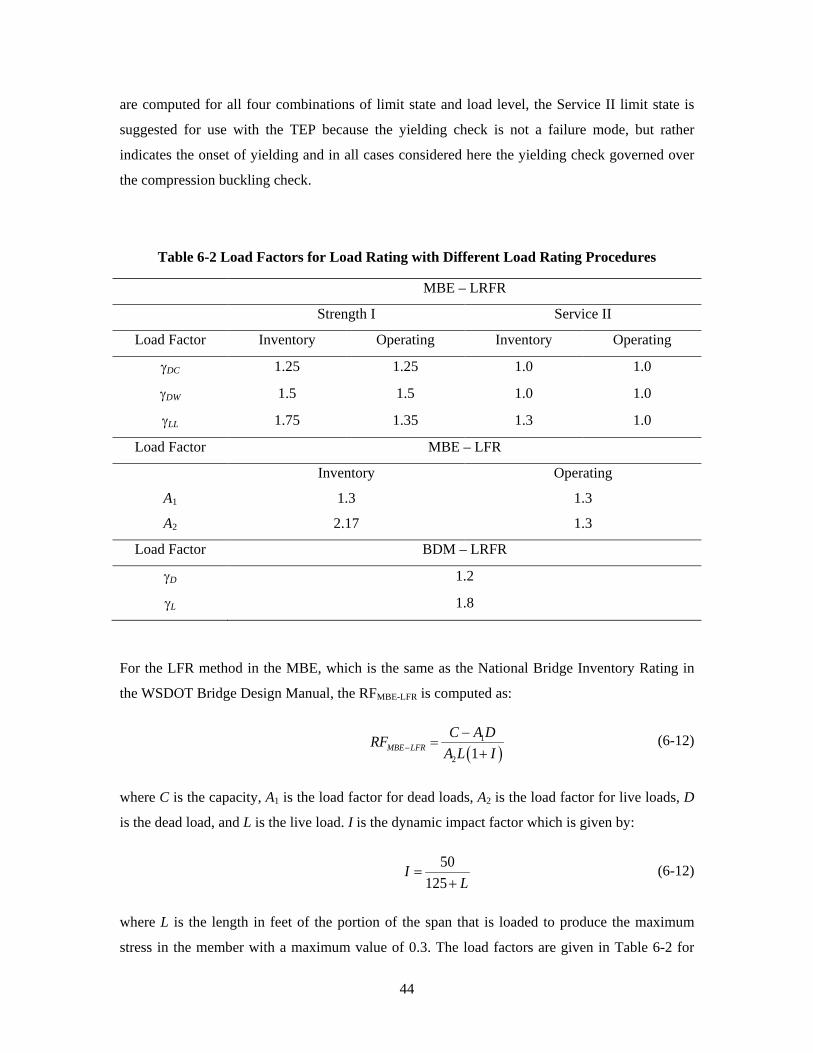
44
are computed for all four combinations of limit state and load level, the Service II limit state is
suggested for use with the TEP because the yielding check is not a failure mode, but rather
indicates the onset of yielding and in all cases considered here the yielding check governed over
the compression buckling check.
Table 6-2 Load Factors for Load Rating with Different Load Rating Procedures
MBE – LRFR
Strength I Service II
Load Factor Inventory Operating Inventory Operating
γDC 1.25 1.25 1.0 1.0
γDW 1.5 1.5 1.0 1.0
γLL 1.75 1.35 1.3 1.0
Load Factor MBE – LFR
Inventory Operating
A1 1.3 1.3
A2 2.17 1.3
Load Factor BDM – LRFR
γD 1.2
γL 1.8
For the LFR method in the MBE, which is the same as the National Bridge Inventory Rating in
the WSDOT Bridge Design Manual, the RFMBE-LFR is computed as:
( )
1
2 1MBE LFRC A DRF
A L I−−
=+
(6-12)
where C is the capacity, A1 is the load factor for dead loads, A2 is the load factor for live loads, D
is the dead load, and L is the live load. I is the dynamic impact factor which is given by:
50125
IL
=+
(6-12)
where L is the length in feet of the portion of the span that is loaded to produce the maximum
stress in the member with a maximum value of 0.3. The load factors are given in Table 6-2 for
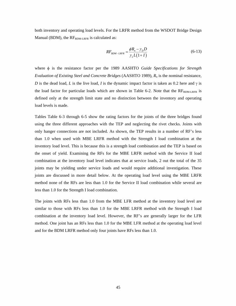
45
both inventory and operating load levels. For the LRFR method from the WSDOT Bridge Design
Manual (BDM), the RFBDM-LRFR is calculated as:
( )1
n DBDM LRFR
L
R DRFL I
φ γγ−
−=
+ (6-13)
where φ is the resistance factor per the 1989 AASHTO Guide Specifications for Strength
Evaluation of Existing Steel and Concrete Bridges (AASHTO 1989), Rn is the nominal resistance,
D is the dead load, L is the live load, I is the dynamic impact factor is taken as 0.2 here and γ is
the load factor for particular loads which are shown in Table 6-2. Note that the RFBDM-LRFR is
defined only at the strength limit state and no distinction between the inventory and operating
load levels is made.
Tables Table 6-3 through 6-5 show the rating factors for the joints of the three bridges found
using the three different approaches with the TEP and neglecting the rivet checks. Joints with
only hanger connections are not included. As shown, the TEP results in a number of RF’s less
than 1.0 when used with MBE LRFR method with the Strength I load combination at the
inventory load level. This is because this is a strength load combination and the TEP is based on
the onset of yield. Examining the RFs for the MBE LRFR method with the Service II load
combination at the inventory load level indicates that at service loads, 2 out the total of the 35
joints may be yielding under service loads and would require additional investigation. These
joints are discussed in more detail below. At the operating load level using the MBE LRFR
method none of the RFs are less than 1.0 for the Service II load combination while several are
less than 1.0 for the Strength I load combination.
The joints with RFs less than 1.0 from the MBE LFR method at the inventory load level are
similar to those with RFs less than 1.0 for the MBE LRFR method with the Strength I load
combination at the inventory load level. However, the RF’s are generally larger for the LFR
method. One joint has an RFs less than 1.0 for the MBE LFR method at the operating load level
and for the BDM LRFR method only four joints have RFs less than 1.0.

46
Table 6-3 Rating Factors for BR 90-134N Joints Using the TEP
MBE - LRFR Strength
I
MBE - LRFR Service
II MBE - LFR
BDM -
LRFR Joint
ID Inventory Operating Inventory Operating Inventory Operating
L2 1.34 1.73 2.20 2.86 1.60 2.67 2.03
L4 1.19 1.54 2.00 2.60 1.44 2.41 1.84
U1 1.49 1.93 2.33 3.03 1.58 2.63 2.15
U3* 0.75 0.97 1.41 1.84 0.99 1.66 1.29
* Indicates joints where all RFs would be greater 1.0 if compressions chords that are milled-to-bear were neglected.
Table 6-4 Rating Factors for BR 31-36 Joints Using the TEP
MBE - LRFR Strength
I
MBE - LRFR Service
II MBE - LFR
BDM -
LRFR Joint
ID Inventory Operating Inventory Operating Inventory Operating
L1 0.75 0.97 1.13 1.46 0.94 1.56 1.15
L3 1.15 1.50 1.82 2.36 1.58 2.64 1.88
L5 1.35 1.75 2.10 2.73 1.59 2.66 1.94
L7 2.57 3.33 3.75 4.87 1.65 2.76 2.03
L9 0.30 0.40 0.78 1.01 0.50 0.84 0.70
L10 1.62 2.11 2.48 3.23 2.06 3.44 2.58
L12 0.94 1.22 1.50 1.95 1.20 2.01 1.55
U2 0.69 0.89 1.02 1.33 0.90 1.50 1.06
U4 1.85 2.40 2.81 3.65 2.19 3.66 2.67
U6 1.19 1.54 1.95 2.54 1.76 2.94 2.09
U8 1.10 1.42 1.84 2.39 1.65 2.76 2.03
U10 3.66 4.74 5.24 6.81 3.22 5.38 3.94
U11 0.59 0.76 1.08 1.41 0.86 1.43 1.12
U13 1.72 2.23 2.61 3.40 1.93 3.22 2.42
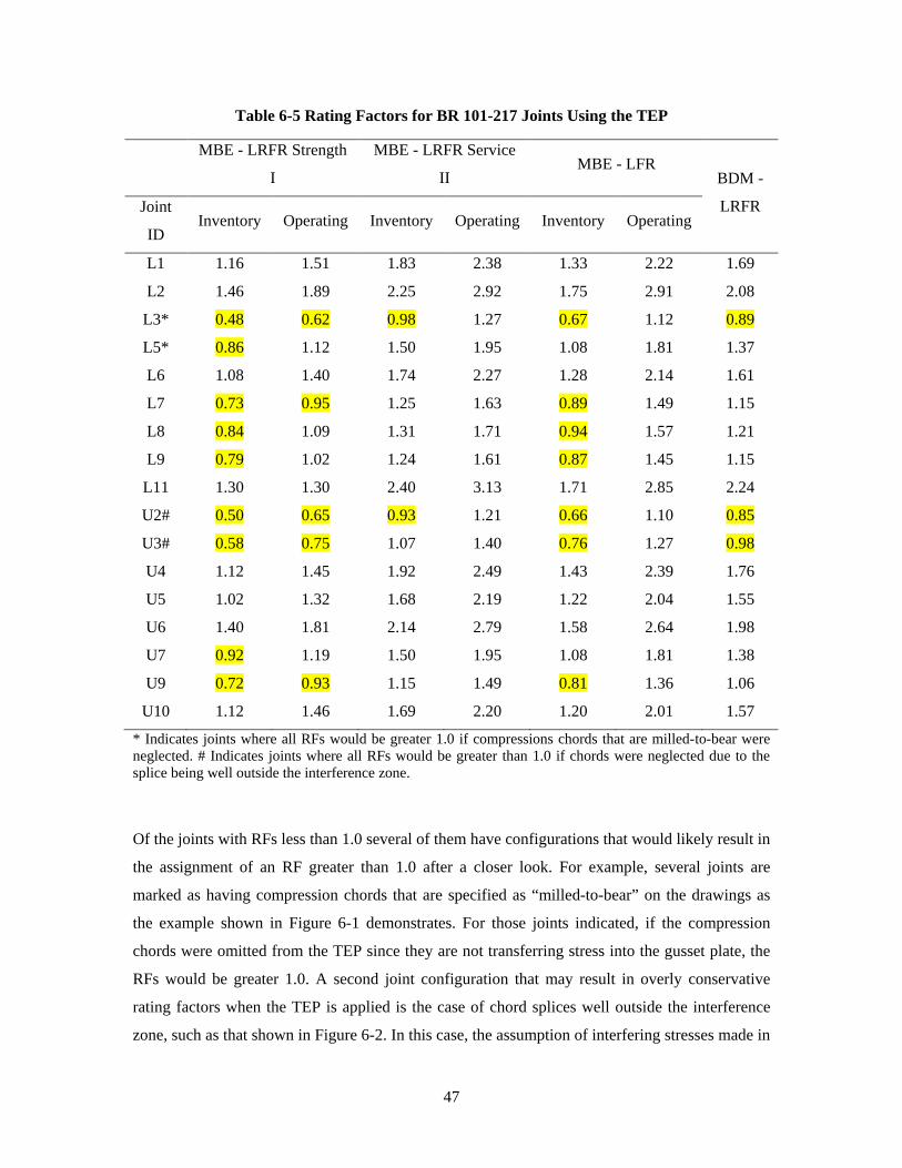
47
Table 6-5 Rating Factors for BR 101-217 Joints Using the TEP
MBE - LRFR Strength
I
MBE - LRFR Service
II MBE - LFR
BDM -
LRFR Joint
ID Inventory Operating Inventory Operating Inventory Operating
L1 1.16 1.51 1.83 2.38 1.33 2.22 1.69
L2 1.46 1.89 2.25 2.92 1.75 2.91 2.08
L3* 0.48 0.62 0.98 1.27 0.67 1.12 0.89
L5* 0.86 1.12 1.50 1.95 1.08 1.81 1.37
L6 1.08 1.40 1.74 2.27 1.28 2.14 1.61
L7 0.73 0.95 1.25 1.63 0.89 1.49 1.15
L8 0.84 1.09 1.31 1.71 0.94 1.57 1.21
L9 0.79 1.02 1.24 1.61 0.87 1.45 1.15
L11 1.30 1.30 2.40 3.13 1.71 2.85 2.24
U2# 0.50 0.65 0.93 1.21 0.66 1.10 0.85
U3# 0.58 0.75 1.07 1.40 0.76 1.27 0.98
U4 1.12 1.45 1.92 2.49 1.43 2.39 1.76
U5 1.02 1.32 1.68 2.19 1.22 2.04 1.55
U6 1.40 1.81 2.14 2.79 1.58 2.64 1.98
U7 0.92 1.19 1.50 1.95 1.08 1.81 1.38
U9 0.72 0.93 1.15 1.49 0.81 1.36 1.06
U10 1.12 1.46 1.69 2.20 1.20 2.01 1.57
* Indicates joints where all RFs would be greater 1.0 if compressions chords that are milled-to-bear were neglected. # Indicates joints where all RFs would be greater than 1.0 if chords were neglected due to the splice being well outside the interference zone.
Of the joints with RFs less than 1.0 several of them have configurations that would likely result in
the assignment of an RF greater than 1.0 after a closer look. For example, several joints are
marked as having compression chords that are specified as “milled-to-bear” on the drawings as
the example shown in Figure 6-1 demonstrates. For those joints indicated, if the compression
chords were omitted from the TEP since they are not transferring stress into the gusset plate, the
RFs would be greater 1.0. A second joint configuration that may result in overly conservative
rating factors when the TEP is applied is the case of chord splices well outside the interference
zone, such as that shown in Figure 6-2. In this case, the assumption of interfering stresses made in

48
the derivation of the TEP yield check is likely overly conservative since the splice is removed
from where the stresses from the diagonal or vertical would be expected to interact. Joints with
these conditions are indicated in Tables Table 6-3 through 6-5. If these joints are considered to
have a RF greater than 1.0, which would be the case given the discussion above, then no joints
are identified as likely to be yielding under in the MBE LRFR method under the Service II load
combination at the inventory load level.
Figure 6-2 Example of Joint with Chords Spliced Outside Interference Zone from BR 101-
217
Figure 6-1 Example of Joint with Milled-to-Bear Compression Chords from BR 101-217.
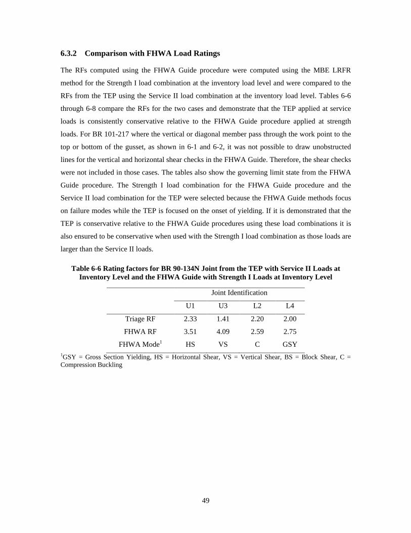
49
6.3.2 Comparison with FHWA Load Ratings
The RFs computed using the FHWA Guide procedure were computed using the MBE LRFR
method for the Strength I load combination at the inventory load level and were compared to the
RFs from the TEP using the Service II load combination at the inventory load level. Tables 6-6
through 6-8 compare the RFs for the two cases and demonstrate that the TEP applied at service
loads is consistently conservative relative to the FHWA Guide procedure applied at strength
loads. For BR 101-217 where the vertical or diagonal member pass through the work point to the
top or bottom of the gusset, as shown in 6-1 and 6-2, it was not possible to draw unobstructed
lines for the vertical and horizontal shear checks in the FHWA Guide. Therefore, the shear checks
were not included in those cases. The tables also show the governing limit state from the FHWA
Guide procedure. The Strength I load combination for the FHWA Guide procedure and the
Service II load combination for the TEP were selected because the FHWA Guide methods focus
on failure modes while the TEP is focused on the onset of yielding. If it is demonstrated that the
TEP is conservative relative to the FHWA Guide procedures using these load combinations it is
also ensured to be conservative when used with the Strength I load combination as those loads are
larger than the Service II loads.
Table 6-6 Rating factors for BR 90-134N Joint from the TEP with Service II Loads at Inventory Level and the FHWA Guide with Strength I Loads at Inventory Level
Joint Identification
U1 U3 L2 L4
Triage RF 2.33 1.41 2.20 2.00
FHWA RF 3.51 4.09 2.59 2.75
FHWA Mode1 HS VS C GSY 1GSY = Gross Section Yielding, HS = Horizontal Shear, VS = Vertical Shear, BS = Block Shear, C = Compression Buckling
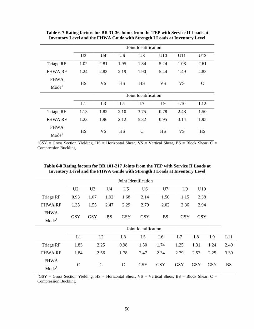
50
Table 6-7 Rating factors for BR 31-36 Joints from the TEP with Service II Loads at Inventory Level and the FHWA Guide with Strength I Loads at Inventory Level
Joint Identification
U2 U4 U6 U8 U10 U11 U13
Triage RF 1.02 2.81 1.95 1.84 5.24 1.08 2.61
FHWA RF 1.24 2.83 2.19 1.90 5.44 1.49 4.85
FHWA
Mode1 HS VS HS HS VS VS C
Joint Identification
L1 L3 L5 L7 L9 L10 L12
Triage RF 1.13 1.82 2.10 3.75 0.78 2.48 1.50
FHWA RF 1.23 1.96 2.12 5.32 0.95 3.14 1.95
FHWA
Mode1 HS VS HS C HS VS HS
1GSY = Gross Section Yielding, HS = Horizontal Shear, VS = Vertical Shear, BS = Block Shear, C = Compression Buckling
Table 6-8 Rating factors for BR 101-217 Joints from the TEP with Service II Loads at Inventory Level and the FHWA Guide with Strength I Loads at Inventory Level
Joint Identification
U2 U3 U4 U5 U6 U7 U9 U10
Triage RF 0.93 1.07 1.92 1.68 2.14 1.50 1.15 2.38
FHWA RF 1.35 1.55 2.47 2.29 2.79 2.02 2.86 2.94
FHWA
Mode1 GSY GSY BS GSY GSY BS GSY GSY
Joint Identification
L1 L2 L3 L5 L6 L7 L8 L9 L11
Triage RF 1.83 2.25 0.98 1.50 1.74 1.25 1.31 1.24 2.40
FHWA RF 1.84 2.56 1.78 2.47 2.34 2.79 2.53 2.25 3.39
FHWA
Mode1 C C C GSY GSY GSY GSY GSY BS
1GSY = Gross Section Yielding, HS = Horizontal Shear, VS = Vertical Shear, BS = Block Shear, C = Compression Buckling
51
The tables above indicate that the single joint of the three bridges considered that has an RF of
less than 1.0 using the FHWA Guide procedures, Joint L9 from BR 31-36, also has an RF of less
than 1.0 from the TEP. Additionally, if the RFs less than 1.0 from the TEP for bridge 101-217 are
not considered as they are resulting from compression chords that are milled-to-bear and tension
chords with splices outside the interference zone, only Joint L9 has an RF of less than 1.0 from
the TEP. Thus, using the TEP at service loads is both conservative relative to the FHWA Guide
approach and is also consistent with the FHWA Guide approach in identifying the same joint as
having insufficient capacity at the inventory load levels. It should be noted that the TEP would be
consistently conservative relative to the FHWA Guide approach for all other rating methods
described in the previous section. Further, the TEP may employed at with strength load
combinations but will generate conservative results. Joints found to RFs less than 1.0 with the
TEP applied at strength load combinations could then be evaluated with the TEP and service
loads to determine whether any additional action might be warranted.
6.3.3 Load Ratings Including Rivets
As discussed, the RFs above do not include rivet shear as a possible limit state so that the gusset
plate checks in the TEP and FHWA Guide could be compared. The FHWA Guide recommends
rivet shear strengths as given in Table 6-9, which depend on the age of the bridge. Given the ages
of the bridges considered here, the rivets for BR 90-134N and BR 31-36 would be assigned a
shear strength of 145 MPa (21 ksi) and the rivets of BR 101-217 would be assigned a shear
strength of 124 MPa (18 ksi). RFs were calculated for the joints of the three bridges using these
shear strengths and only the rivet limit state. The resulting RFs are shown in Tables 6-10 through
Table 6-12 for the MBE LRFR rating method and the MBE LFR method. As shown almost all
the RFs found only from the rivet shear strength are smaller than RFs for the gusset plate limit
states. Further, many of the RFs are less than 1.0, with only one joint having an RF greater 1.0 for
the MBE LRFR rating method at the Strength I limit state and inventory load level and only three
joints have RFs greater 1.0 for the MBE LFR rating method at the inventory load levels. BR 101-
217 has many RFs less than 1.0 for all rating methods and load levels. These results indicate that
either many of the rivets on these bridges need replacement or that the recommended rivet
strengths are too low.
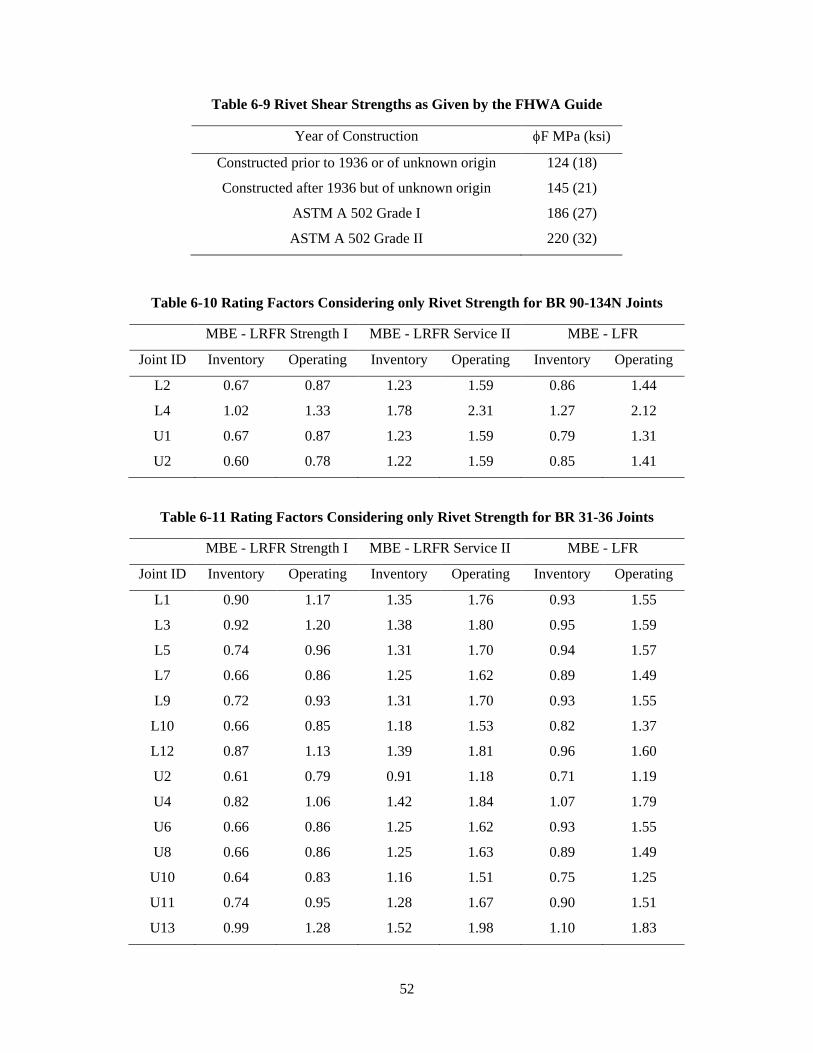
52
Table 6-9 Rivet Shear Strengths as Given by the FHWA Guide
Year of Construction φF MPa (ksi)
Constructed prior to 1936 or of unknown origin 124 (18)
Constructed after 1936 but of unknown origin 145 (21)
ASTM A 502 Grade I 186 (27)
ASTM A 502 Grade II 220 (32)
Table 6-10 Rating Factors Considering only Rivet Strength for BR 90-134N Joints
MBE - LRFR Strength I MBE - LRFR Service II MBE - LFR
Joint ID Inventory Operating Inventory Operating Inventory Operating
L2 0.67 0.87 1.23 1.59 0.86 1.44
L4 1.02 1.33 1.78 2.31 1.27 2.12
U1 0.67 0.87 1.23 1.59 0.79 1.31
U2 0.60 0.78 1.22 1.59 0.85 1.41
Table 6-11 Rating Factors Considering only Rivet Strength for BR 31-36 Joints
MBE - LRFR Strength I MBE - LRFR Service II MBE - LFR
Joint ID Inventory Operating Inventory Operating Inventory Operating
L1 0.90 1.17 1.35 1.76 0.93 1.55
L3 0.92 1.20 1.38 1.80 0.95 1.59
L5 0.74 0.96 1.31 1.70 0.94 1.57
L7 0.66 0.86 1.25 1.62 0.89 1.49
L9 0.72 0.93 1.31 1.70 0.93 1.55
L10 0.66 0.85 1.18 1.53 0.82 1.37
L12 0.87 1.13 1.39 1.81 0.96 1.60
U2 0.61 0.79 0.91 1.18 0.71 1.19
U4 0.82 1.06 1.42 1.84 1.07 1.79
U6 0.66 0.86 1.25 1.62 0.93 1.55
U8 0.66 0.86 1.25 1.63 0.89 1.49
U10 0.64 0.83 1.16 1.51 0.75 1.25
U11 0.74 0.95 1.28 1.67 0.90 1.51
U13 0.99 1.28 1.52 1.98 1.10 1.83
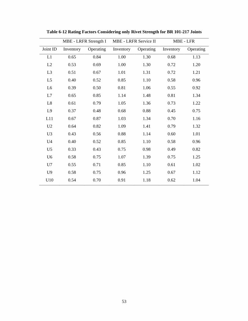
53
Table 6-12 Rating Factors Considering only Rivet Strength for BR 101-217 Joints
MBE - LRFR Strength I MBE - LRFR Service II MBE - LFR
Joint ID Inventory Operating Inventory Operating Inventory Operating
L1 0.65 0.84 1.00 1.30 0.68 1.13
L2 0.53 0.69 1.00 1.30 0.72 1.20
L3 0.51 0.67 1.01 1.31 0.72 1.21
L5 0.40 0.52 0.85 1.10 0.58 0.96
L6 0.39 0.50 0.81 1.06 0.55 0.92
L7 0.65 0.85 1.14 1.48 0.81 1.34
L8 0.61 0.79 1.05 1.36 0.73 1.22
L9 0.37 0.48 0.68 0.88 0.45 0.75
L11 0.67 0.87 1.03 1.34 0.70 1.16
U2 0.64 0.82 1.09 1.41 0.79 1.32
U3 0.43 0.56 0.88 1.14 0.60 1.01
U4 0.40 0.52 0.85 1.10 0.58 0.96
U5 0.33 0.43 0.75 0.98 0.49 0.82
U6 0.58 0.75 1.07 1.39 0.75 1.25
U7 0.55 0.71 0.85 1.10 0.61 1.02
U9 0.58 0.75 0.96 1.25 0.67 1.12
U10 0.54 0.70 0.91 1.18 0.62 1.04

54
Section 7 Historical Evaluation of Rivet Strength
7.1 Historical Rivet Testing Programs
A preliminary investigation of the rivet shear strength recommended in the FHWA Guide
including a survey of literature on the testing of riveted joints was conducted. Data was gathered
from experiments conducted from 1904-1941 on a variety of riveted joints having various
configurations, rivet materials and plate materials. The experimental programs are briefly
summarized below followed by a discussion of their results.
The American Railway Engineering and Maintenance-of-Way Association (AREMA) conducted
tests on various joint configurations, from single rivet joints to joints with multiple rivets and
layered splice plates (AREMA 1904), for a total of 90 individual tests. Both the rivet and plate
material was specified as Open-Hearth (OH) steel. Force-displacement plots were recorded for
all joints and rivet shear stresses for each joint were calculated assuming an even distribution of
load to each rivet. Connections were tested to failure of either the rivets or the plates.
Talbot and Moore (1911) tested joints that were modeled after the AREMA (1904) tests but had
different rivet materials. They conducted 90 tests on joints with rivets made with nickel-steel and
54 tests on joints with chrome-nickel steel. Total force and connection deformation were recorded
and the loads were assumed to be evenly distributed to the rivets for calculating the individual
rivet stress. Connections were again tested to failure.
Davis et al. (1939) tested 37 different joint configurations where the number of rivets and number
of splice plates were varied between specimens. The rivet and plate materials were also varied
with both carbon-steel and manganese-steel rivets investigated. Davis et al. introduced the
concept of effective rivet yield (ERY) discussed below and outlined the general behavior of rivets
through failure. All connections were tested to failure and the load was again assumed to be
evenly distributed to each rivet.
Wilson et al. (1941) tested 63 joints in seven different joint configurations. Three different low
alloy steels (denoted A, B and C) were used for the rivets. Munse and Cox (1956) tested
individual rivets without driving them into holes in a setup that could subject the rivets to varying
degrees of combined tension and shear. The rivet diameter and grip length were also varied. From
this extensive testing program data on 44 rivets loaded only in shear was obtained.
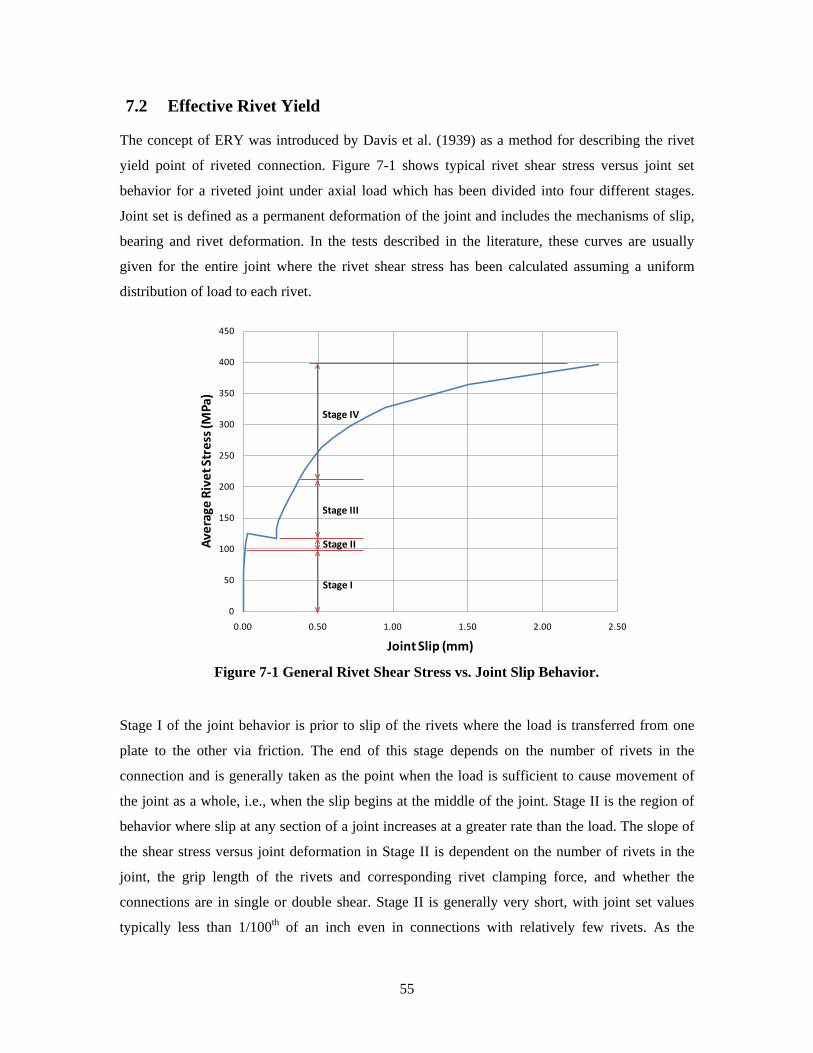
55
7.2 Effective Rivet Yield
The concept of ERY was introduced by Davis et al. (1939) as a method for describing the rivet
yield point of riveted connection. Figure 7-1 shows typical rivet shear stress versus joint set
behavior for a riveted joint under axial load which has been divided into four different stages.
Joint set is defined as a permanent deformation of the joint and includes the mechanisms of slip,
bearing and rivet deformation. In the tests described in the literature, these curves are usually
given for the entire joint where the rivet shear stress has been calculated assuming a uniform
distribution of load to each rivet.
Stage I of the joint behavior is prior to slip of the rivets where the load is transferred from one
plate to the other via friction. The end of this stage depends on the number of rivets in the
connection and is generally taken as the point when the load is sufficient to cause movement of
the joint as a whole, i.e., when the slip begins at the middle of the joint. Stage II is the region of
behavior where slip at any section of a joint increases at a greater rate than the load. The slope of
the shear stress versus joint deformation in Stage II is dependent on the number of rivets in the
joint, the grip length of the rivets and corresponding rivet clamping force, and whether the
connections are in single or double shear. Stage II is generally very short, with joint set values
typically less than 1/100th of an inch even in connections with relatively few rivets. As the
Figure 7-1 General Rivet Shear Stress vs. Joint Slip Behavior.
0
50
100
150
200
250
300
350
400
450
0.00 0.50 1.00 1.50 2.00 2.50
Aver
age
Rive
t Str
ess (
MPa
)
Joint Slip (mm)
Stage I
Stage II
Stage III
Stage IV
56
number of rivets increases the stiffness of the connection in Stage II will also increase. Stage III is
the region of behavior where the rivets are transferring load largely through bearing which
generally results in a large increase in the joint stiffness and is again dependent on the connection
configuration. Stage IV begins when yielding occurs in plates, rivets, or both and joint set again
increases more rapidly with load. For “over-riveted joints” yielding occurs in plates and for
“under-riveted joints” yielding occurs in rivets. The transition from Stage III to Stage IV is
defined as the ERY and occurs when the stiffness of the joint is ½ of the initial Stage III stiffness.
Following ERY, the connections reach a peak capacity where either the rivets fracture or the
connected plates fracture.
7.3 Collected Rivet Connection Data
Table 7-1 shows the collected data from the testing programs described above. The table included
information on the rivet steel’s basic tensile properties including yield and tensile strengths, the
number of joints tests where data was used to compute ERY and the resulting statistics for ERY,
and the number of joints where data on ultimate rivet shear strength was collected and the
resulting statistics. Note that only joints where rivet fracture was the governing failure mode were
included in the latter, thus the number of tests used for computing ERY and ultimate rivet shear
stress, Vu, are not the same. Further, ERY is not reported for the tests by Munse and Cox (1956)
because they did not give full shear stress or force versus joint set results and only reported
ultimate rivet strengths. ERY was computed for each test by digitizing the rivet shear stress
versus joint set curves using scanned figures and a software program capable of converting pixel
data for a xy plot to numerical data.
Comparing the collected data shown in Table 7-1 with the recommended FHWA values, which
for convenience are repeated at the bottom of Table 7-1, demonstrates that the strength
recommended by FHWA may be overly conservative. It seems that the recommended strengths
align better with ERY than with the ultimate strengths of riveted joints. It should be noted that
this analysis does not consider two important items: (i) the strength of existing rivets after years
in service and the effects of the corrosion that may be present, and (ii) the calibration of the
resistance factor, φ, that is included in the FHWA values. However, the FHWA values are
recommended for use in checking connections at the Strength I load combination where ultimate
strengths and failure modes are typically used as limit states. From the data presented here, it
appears that the recommended values may be overly conservative for that application. Additional
rivet testing is necessary to make recommendations regarding the rivet strengths that should be
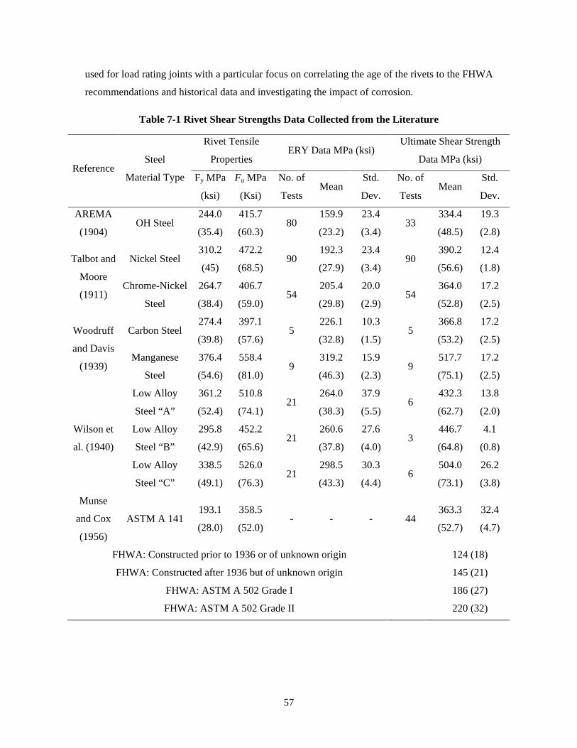
57
used for load rating joints with a particular focus on correlating the age of the rivets to the FHWA
recommendations and historical data and investigating the impact of corrosion.
Table 7-1 Rivet Shear Strengths Data Collected from the Literature
Reference Steel
Material Type
Rivet Tensile
Properties ERY Data MPa (ksi)
Ultimate Shear Strength
Data MPa (ksi)
Fy MPa
(ksi)
Fu MPa
(Ksi)
No. of
Tests Mean
Std.
Dev.
No. of
Tests Mean
Std.
Dev.
AREMA
(1904) OH Steel
244.0
(35.4)
415.7
(60.3) 80
159.9
(23.2)
23.4
(3.4) 33
334.4
(48.5)
19.3
(2.8)
Talbot and
Moore
(1911)
Nickel Steel 310.2
(45)
472.2
(68.5) 90
192.3
(27.9)
23.4
(3.4) 90
390.2
(56.6)
12.4
(1.8)
Chrome-Nickel
Steel
264.7
(38.4)
406.7
(59.0) 54
205.4
(29.8)
20.0
(2.9) 54
364.0
(52.8)
17.2
(2.5)
Woodruff
and Davis
(1939)
Carbon Steel 274.4
(39.8)
397.1
(57.6) 5
226.1
(32.8)
10.3
(1.5) 5
366.8
(53.2)
17.2
(2.5)
Manganese
Steel
376.4
(54.6)
558.4
(81.0) 9
319.2
(46.3)
15.9
(2.3) 9
517.7
(75.1)
17.2
(2.5)
Wilson et
al. (1940)
Low Alloy
Steel “A”
361.2
(52.4)
510.8
(74.1) 21
264.0
(38.3)
37.9
(5.5) 6
432.3
(62.7)
13.8
(2.0)
Low Alloy
Steel “B”
295.8
(42.9)
452.2
(65.6) 21
260.6
(37.8)
27.6
(4.0) 3
446.7
(64.8)
4.1
(0.8)
Low Alloy
Steel “C”
338.5
(49.1)
526.0
(76.3) 21
298.5
(43.3)
30.3
(4.4) 6
504.0
(73.1)
26.2
(3.8)
Munse
and Cox
(1956)
ASTM A 141 193.1
(28.0)
358.5
(52.0) - - - 44
363.3
(52.7)
32.4
(4.7)
FHWA: Constructed prior to 1936 or of unknown origin 124 (18)
FHWA: Constructed after 1936 but of unknown origin 145 (21)
FHWA: ASTM A 502 Grade I 186 (27)
FHWA: ASTM A 502 Grade II 220 (32)
58
Section 8 Conclusions and Recommendations
8.1 Conclusions
The currently recommended FHWA procedures for gusset plate evaluation may not identify all
gusset plates in steel truss bridges that may be yielding under service loads. Analysis results
indicate that a complex interaction of stresses is generated in gusset plates by connecting
members and that this interaction can initiate gusset plate yielding when the uniaxial stresses on
Whitmore sections associated with those connecting members are well below yield. Simple
mechanics were used to develop a conservative and considerably simpler process for identifying
gusset plates that may be yielding of buckling. Gusset plates failing this triage evaluation
procedure may still be adequate, but require more detailed evaluation. Detailed finite element
analysis indicated this method conservatively predicted the onset of gusset plate yielding and was
consistently conservative relative to the procedures in the FHWA Guide, but it is quicker and
easier than the FHWA method. This is the yield check of the recommended Triage Evaluation
Procedure (TEP) for which an automated spreadsheet has been developed and is described in the
Appendix.
Gusset plate buckling did not occur prior to gusset plate yielding in any of the connections
studied at their actual gusset plate thicknesses. When buckling may be a concern, the Modified
Thornton Method of evaluating the gusset plate unbraced length and compressive stress, along
with an effective length factor of 1.0, was found to be conservative when used with the AASHTO
buckling equations. This method is included as the buckling check in the TEP and automated
spreadsheet.
When applied to three bridges in Washington State, the proposed TEP was found to be simple
and appropriately conservative. It resulted in rating factors (RFs) that were conservative relative
to those values in the FHWA Guide and when applied at service loads or operating load levels
very few joints were identified as needing further investigation (i.e., having an RF less than 1.0).
When the rivet strengths recommended in the FHWA Guide were employed to calculate RFs, it
was shown that many joints of the three bridges considered had RFs less than 1.0. Comparison of
the recommended rivet strengths with strengths obtained from experimental results in the
literature indicate that the recommended values may be overly conservative, although additional
research is necessary including experiments on rivets after years of service.
59
8.2 Recommendations
The TEP and automated spreadsheet are recommended for load rating joints in truss bridges for
the limit states of the onset of gusset plate yielding and gusset plate compressive buckling. Rivet
shear strength should also be evaluated and until additional research is completed the values
recommended in the FHWA Guide seem to provide a very conservative lower bound.
8.3 Recommendations for Future Research
The assessment of rivet strength in older steel truss bridges and a comparison with historical data
on the strength of like new rivets is a critical area for future research. As shown here, the rating
factors for a majority of joints on the three truss bridges studied were less than 1.0 and controlled
by the rivet strength when current strength recommendations from the FHWA Guide were used.
A brief literature review demonstrated that the current recommendations are very conservative
relative to historical tests data. However, that historical data is based on tests of pristine
connections built in laboratory conditions. Those strengths may be different than those found
from testing joints in existing bridges. Thus, it is recommended that a study of the strength of
rivets from existing construction be conducted to develop appropriate recommendations.
A refined evaluation procedure for use on those joints that are identified as likely yielding under
service loads in the TEP is necessary. The refined procedure should eliminate some of the
conservative assumptions used to develop the yield check of the TEP. Such a procedure would be
a simple second step for those joints identified as likely yielding.
The impact of layered splice plates on the transfer and distribution of stress in gusset plates is not
understood and should be investigated. Such layered connections were outside the scope of this
project but there are many examples of such connections in the bridge inventory. Current practice
with the use of the procedures in the FHWA Guide is to simply add the area of the plates together
when they overlap in regions being evaluated for the shear check and Whitmore check. However,
this assumes that the stresses in the plates are equal, which may not be the case. Further, the
impact of the layered gusset plates on buckling is not well understood. Currently the plates are
treated as a fully composite member, which may overestimate the buckling strength if instead the
act as completely separate members.
Finally, a detailed study of the effect of corrosion in the critical regions of the gusset plate where
the stresses generated from connecting elements interfere with each other is necessary. Corrosion
in this area is common, especially for lower chord members in though-trusses where water can

60
build up from rain and traffic splashing. The impact of corrosion in this region is difficult to
determine because crack initiation is possible but the gusset plates may also be able to redistribute
stresses around the areas of reduced thickness. Simple methods for assessing the impact are
conceivable and include simply using the reduced thickness. However, it is unclear at this time if
such methods would be overly conservative.

61
Section 9 References
AASHTO (2007). LRFD Bridge Design Specifications, American Association of State Highway and Transportation Officials.
AASHTO (2008), Manual for Bridge Evaluation, 1st Edition, American Association of State Highway and Transportation Officials.
AISC (2002), Specifications for Structural Steel Buildings, American Institute of Steel Construction.
Astaneh-Asl, A, (1989) “Simple Methods for Design of Gusset Plates,” Proceedings ASCE Structures Conference, San Francisco, CA, p345-354
ANSYS (2008), ANSYS Release 11 Reference Manual, ANSYS, Inc.
AREMA (1904). “Tests of Riveted Joints”, American Railway Engineering and Maintenance-of-Way Association, Proceedings, Vol. 6, p272-484.
ASTM (1924). ASTM A7 Standard Specifications for Structural Steel for Bridges. American Society for Testing and Materials.
ASTM (1939). ASTM A7-39 Standard Specifications for Structural Steel for Buildings and Bridges. American Society for Testing and Materials.
ASTM (1946). ASMT A94-46 Standard Specifications for Structural Silicon Steel. American Society for Testing and Materials.
Bjorhovde, R., and Chakrabarti, S. K., (1985) “Test of Full Size Gusset Plate Connections”, ASCE, Journal of Structural Engineering, Vol. 111, No. 3, p667- 684.
Brockenbrough, R.L., (2002) Design Guide 15: AISC Rehabilitation and Retrofit Guide, American Institute of Steel Construction.
Brown, V. L. S., (1998) “Stability of Gusseted Connections in Steel Structures”, Doctoral Dissertation, University of Delaware
CSI (2008). SAP2000 Linear and Nonlinear Static and Dynamic Analysis and Design of Three-Dimensional Structures, Reference Manual, Computers and Structures, Inc.
Davis, R.E., Woodruff, G.B., and Davis, H.E., (1939) “Tension Tests of Large Riveted Joints”, ASCE, Transaction of the American Society of Civil Engineers, Vol. 105, No. 2084, p1193-1299.
FHWA (2009). Load Rating Guidance and Examples for Bolted and Riveted Gusset Plates in Truss Bridges. Publication No. FHWA-IF-09-014, Federal Highway Administration.
Hardash, S.G. and Bjorhovde, R., (1985) “New Design Criteria for Gusset Plate in Tension”, AISC, Engineering Journal, Vol. 22, No. 2, p77-94
Higgins, C., Senturk, A.E., and Turan, O.T. (2010). “Comparison of Block Shear and Whitmore Section Methods for Load Rating Existing Steel Truss Gusset Plate Connections”, Journal of Bridge Engineering, Vol 15, No. 2, p160-171.

62
Munse, W.H., and Cox, H.L. (1956) “The Static Strength of Rivets Subjected to Combined Tension and Shear”, University of Illinois, Bulletins of the Engineering Experiment Station, No. 437.
NTSB (2008), “Structural Investigation Group Chairman Factual Report, Report No. 08-115,” National Transportation Safety Board, Washington D.C., March 5, 2008.
Ocel, J.M. and Wright, W.J. (2008). Finite Element Modeling of I-35 Bridge Collapse, Final Report, Turner-Fairbank Highway Research Center Report, Federal Highway Administration.
Olson, A.W. (2010). “Triage Evaluation of Gusset Plates in Steel Truss Bridges”, MSCE Thesis, University of Washington.
Roeder, C.W., Lehman, D.E., and Yoo, J.H., (2005) "Improved Seismic Design of Steel Frame Connections," International Journal of Steel Structures, Korean Society of Steel Construction, Seoul, Korea, Vol. 5, No. 2, pgs 141-53.
Sheng, N., Yam, M. C. H., and Lu, V.P., (2002) “Analytical Investigation and the Design of the Compressive Strength of Steel Gusset Plate Connections”, Journal of Constructional Steel Research, v 58, p 1473-1493
Talbot, A.N. and Moore, H.F. (1911) “Tests of Nickel-Steel Riveted Joints”, University of Illinois, Bulletins of the Engineering Experiment Station, Vol. 7, No. 49, p1-53.
Thornton, W.A., (1984) “Bracing Connections for Heavy Construction”, AISC, Engineering Journal, Vol. 21, No 3, p139-148
WSDOT (2010). Bridge Design Manual LRFD, Washington State Department of Transportation.
Whitmore, R.E., (1952) “Experimental Investigation of Stresses in Gusset Plates”, Bulletin NO. 16, Engineering experiment station, University of Tennessee.
Wilson, W.M., Bruckner, W.H., and McCrackin, T.H., (1942) “Tests of Riveted and Welded Joints in Low-Alloy Structural Steels”, University of Illinois, Bulletins of the Engineering Experiment Station, No. 337.
Yam, M.C.H. (1994). “Compressive Behavior and Strength of Steel Gusset Plate Connections.” Doctoral Dissertation, University of Alberta.
Yam, M. C. H, and Cheng, J. J. R., (2002) “Behavior and Design of Gusset Plate Connections in Compression”, Journal of Constructional Steel Research, v 58, n 5-8, p 1143-1159
Yoo, J.H. (2006). “Analytical Investigation on the Seismic Performance of Special Concentrically Braced Frames”, Ph.D. Dissertation, University of Washington.
Yoo, J.H., Roeder, C.W., and Lehman, D.E., (2008) "FEM Simulation and Failure Analysis of Special Concentrically Braced Frame Tests," ASCE, Journal of Structural Engineering, Vol.134, No. 6, Reston, VA, pgs 881-89.
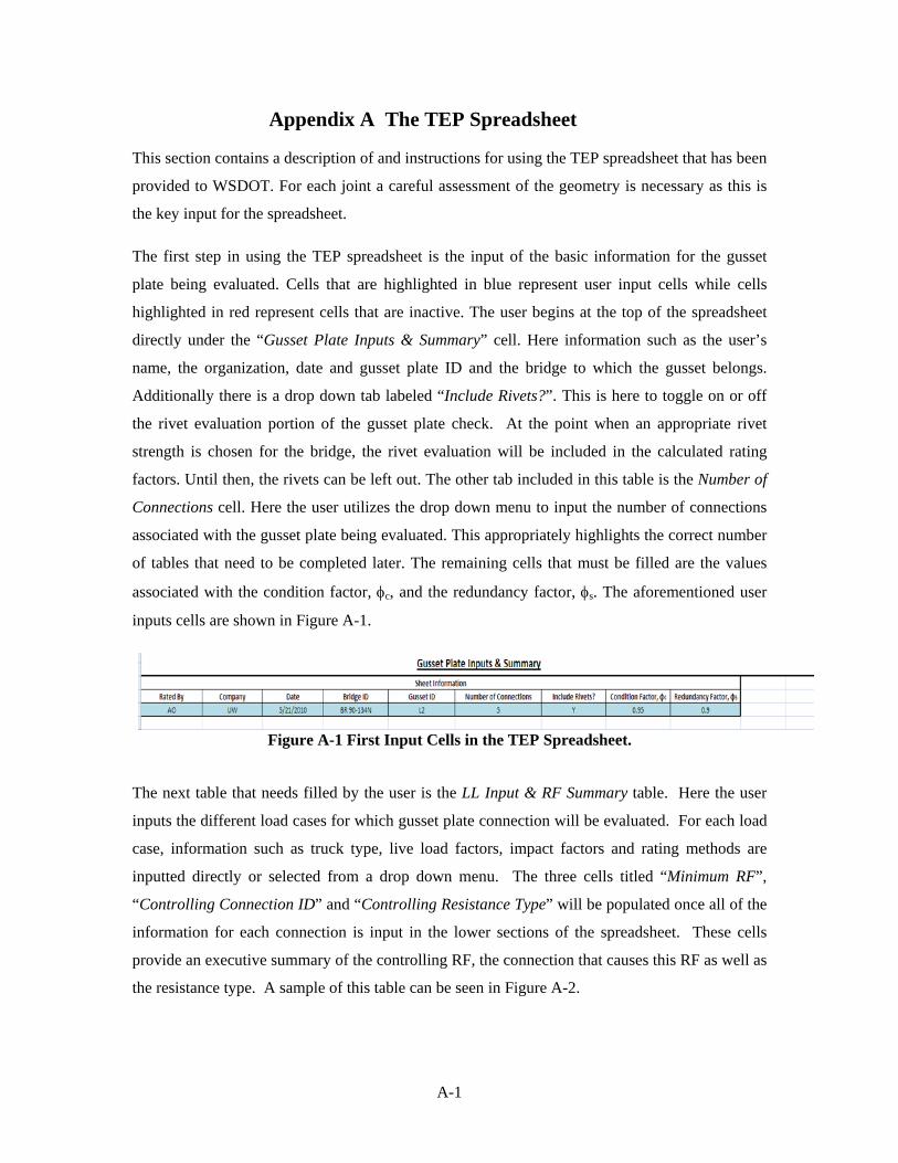
A-1
Appendix A The TEP Spreadsheet
This section contains a description of and instructions for using the TEP spreadsheet that has been
provided to WSDOT. For each joint a careful assessment of the geometry is necessary as this is
the key input for the spreadsheet.
The first step in using the TEP spreadsheet is the input of the basic information for the gusset
plate being evaluated. Cells that are highlighted in blue represent user input cells while cells
highlighted in red represent cells that are inactive. The user begins at the top of the spreadsheet
directly under the “Gusset Plate Inputs & Summary” cell. Here information such as the user’s
name, the organization, date and gusset plate ID and the bridge to which the gusset belongs.
Additionally there is a drop down tab labeled “Include Rivets?”. This is here to toggle on or off
the rivet evaluation portion of the gusset plate check. At the point when an appropriate rivet
strength is chosen for the bridge, the rivet evaluation will be included in the calculated rating
factors. Until then, the rivets can be left out. The other tab included in this table is the Number of
Connections cell. Here the user utilizes the drop down menu to input the number of connections
associated with the gusset plate being evaluated. This appropriately highlights the correct number
of tables that need to be completed later. The remaining cells that must be filled are the values
associated with the condition factor, φc, and the redundancy factor, φs. The aforementioned user
inputs cells are shown in Figure A-1.
The next table that needs filled by the user is the LL Input & RF Summary table. Here the user
inputs the different load cases for which gusset plate connection will be evaluated. For each load
case, information such as truck type, live load factors, impact factors and rating methods are
inputted directly or selected from a drop down menu. The three cells titled “Minimum RF”,
“Controlling Connection ID” and “Controlling Resistance Type” will be populated once all of the
information for each connection is input in the lower sections of the spreadsheet. These cells
provide an executive summary of the controlling RF, the connection that causes this RF as well as
the resistance type. A sample of this table can be seen in Figure A-2.
Figure A-1 First Input Cells in the TEP Spreadsheet.

A-2
The next table that must be completed by the user is the “Material & Dimension” table. Here the
user inputs the yield strengths for the gusset plates and splice plates as well as the ultimate
strength of the rivets as shown in Figure A-3. The rivet strength cell may be inactive depending
on the selection of the “Include Rivets?” cell as discussed before. Additionally there are inputs
for the number of main gusset plates as well as their thicknesses.
Once the user has input the appropriate values into the preceding tables, evaluation of each
connection in the gusset plate begins. This starts by using the “Connection Information” table
under the “Triage Procedure Connection Inputs” section shown in Figure A-4. The first input is
the “Connection ID” cell. As an example the connection for the member from Joint L1 to Joint
L0 is being evaluated. Next the user selects whether the connection corresponds to a chord or
web member using the dropdown menu in the “Chord or Web?” cell. All diagonals and verticals
are considered web members. Next the user uses the drop down menus in the “Splice PL’s?” and
Figure A-4 Connection Information Input in the TEP Spreadsheet.
Figure A-3 Gusset Plate Property Input in the TEP Spreadsheet.
Figure A-2 LL Input and RF Summary Table in the TEP Spreadsheet.

A-3
“Wind Bracing GP?” cells to include or exclude the appropriate areas of these supplemental
plates for the triage procedure calculation of the chord splices. The next cell, “Comp. or
Tension?” triggers the inclusion of the buckling check which will be discussed later in these
instructions. The final cell in the row is titled “Milled to Bear?”. This cell can only be triggered
when the connection corresponds with a chord that is in compression. If “Y” is selected for this
cell than the evaluation of the gusset for the chord splice can be stopped because the member is
milled to bear and thus the triage approach does not apply since gusset plate buckling is not
possible and the rivets provide little to no load transfer. If this is the case, the user can proceed
directly to the next connection on the gusset plate (i.e., the connection of a web member to the
gusset plate under consideration), otherwise if “N” is selected, than the evaluation proceeds as
normal.
The next step in the “Triage Procedure Connection Inputs” section is to calculate the yield
resistance of the gusset plate connection. This starts by inputting the basic geometry of the
connection itself. Parameters such as connection width, , connection length, , and edge
length, , are input into their respective cells. It should be noted that the edge length cell will
only be active for chord member connections, otherwise this cell will be shaded red.
Next the user inputs the information associated with any splice plates used in the connection.
Parameters like splice identification, plate width and thickness are input into the “Splice ID”,
“ ”, and “ ” cells, respectively. These splice plate input cells will only be activated if the
user has input “Y” in the “Splice PL’s” cell, as previously described.
Finally the user inputs parameters associated with any wind bracing gusset plates into the “Wind
Brace GP Dimensions” table, if this table has been activated by inputting “Y” in the “Wind
Bracing GP” cell. Here information such as brace identification, connection width, connection
length, edge distance and wind plate thickness are inputted into the appropriate cells.
Now that all of the pertinent information for the yielding portion of the TEP check have been
completed, a resistance, , will be calculated for this connection and is displayed at the end of
the section. A sample of the yielding calculation for a gusset plate connection is shown in Figure
A-6.
The next section in the connection check is the “Buckling Resistance Inputs” section, shown
below in Figure A-6. Note that this section is only triggered for members in compression that are
not milled to bear. Here the only main user input is the centroidal buckling length in the
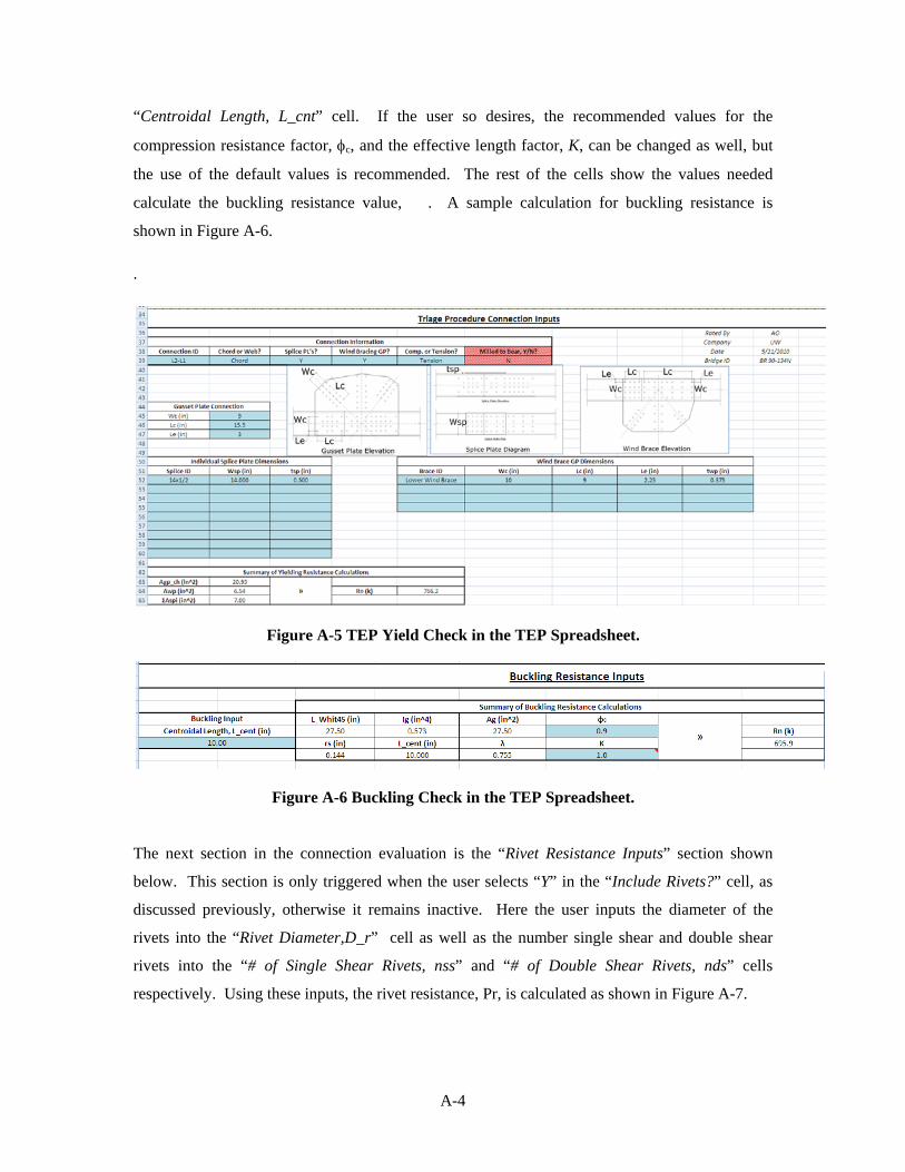
A-4
“Centroidal Length, L_cnt” cell. If the user so desires, the recommended values for the
compression resistance factor, φc, and the effective length factor, K, can be changed as well, but
the use of the default values is recommended. The rest of the cells show the values needed
calculate the buckling resistance value, . A sample calculation for buckling resistance is
shown in Figure A-6.
.
The next section in the connection evaluation is the “Rivet Resistance Inputs” section shown
below. This section is only triggered when the user selects “Y” in the “Include Rivets?” cell, as
discussed previously, otherwise it remains inactive. Here the user inputs the diameter of the
rivets into the “Rivet Diameter,D_r” cell as well as the number single shear and double shear
rivets into the “# of Single Shear Rivets, nss” and “# of Double Shear Rivets, nds” cells
respectively. Using these inputs, the rivet resistance, Pr, is calculated as shown in Figure A-7.
Figure A-6 Buckling Check in the TEP Spreadsheet.
Figure A-5 TEP Yield Check in the TEP Spreadsheet.
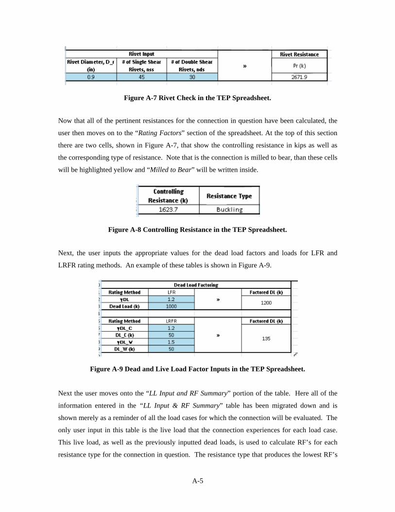
A-5
Now that all of the pertinent resistances for the connection in question have been calculated, the
user then moves on to the “Rating Factors” section of the spreadsheet. At the top of this section
there are two cells, shown in Figure A-7, that show the controlling resistance in kips as well as
the corresponding type of resistance. Note that is the connection is milled to bear, than these cells
will be highlighted yellow and “Milled to Bear” will be written inside.
Next, the user inputs the appropriate values for the dead load factors and loads for LFR and
LRFR rating methods. An example of these tables is shown in Figure A-9.
Next the user moves onto the “LL Input and RF Summary” portion of the table. Here all of the
information entered in the “LL Input & RF Summary” table has been migrated down and is
shown merely as a reminder of all the load cases for which the connection will be evaluated. The
only user input in this table is the live load that the connection experiences for each load case.
This live load, as well as the previously inputted dead loads, is used to calculate RF’s for each
resistance type for the connection in question. The resistance type that produces the lowest RF’s
Figure A-9 Dead and Live Load Factor Inputs in the TEP Spreadsheet.
Figure A-8 Controlling Resistance in the TEP Spreadsheet.
Figure A-7 Rivet Check in the TEP Spreadsheet.
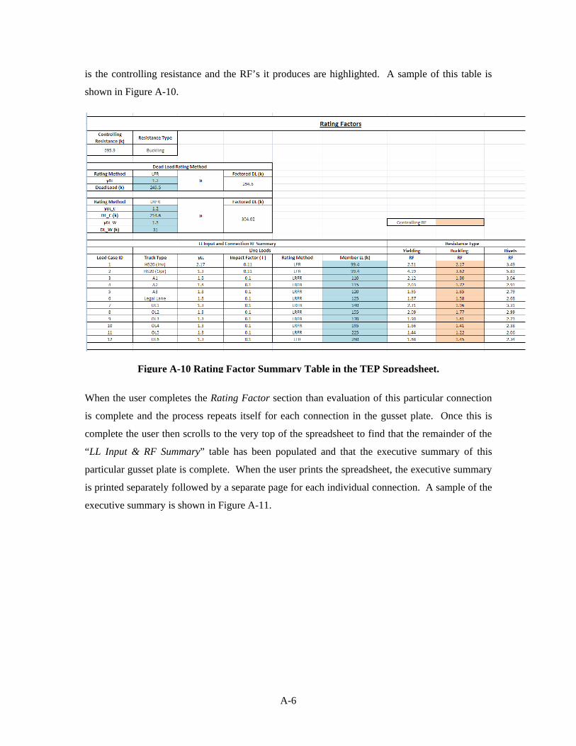
A-6
is the controlling resistance and the RF’s it produces are highlighted. A sample of this table is
shown in Figure A-10.
When the user completes the Rating Factor section than evaluation of this particular connection
is complete and the process repeats itself for each connection in the gusset plate. Once this is
complete the user then scrolls to the very top of the spreadsheet to find that the remainder of the
“LL Input & RF Summary” table has been populated and that the executive summary of this
particular gusset plate is complete. When the user prints the spreadsheet, the executive summary
is printed separately followed by a separate page for each individual connection. A sample of the
executive summary is shown in Figure A-11.
Figure A-10 Rating Factor Summary Table in the TEP Spreadsheet.
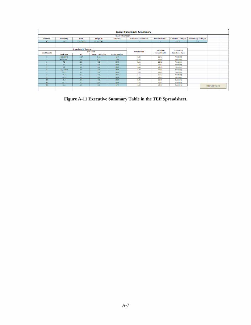
A-7
Figure A-11 Executive Summary Table in the TEP Spreadsheet.
Top Related