


Languages
Pages
Legal

I
Topology Optimisation of Composites with Base Materials of Distinct Poisson’s Ratios
A thesissubmitted in fulfilment of the requirements for the degree of MasterofEngineering
XuranDu
Bachelor of Engineering, China University of Mining and Technology (Beijing), China
School of Engineering.
College of Science, Engineering and Health.
RMIT University
July2017

Topology Optimisation of Composites with Base Materials of Distinct Poisson’s Ratios
II
Declaration
I certify that except where due acknowledgement has been made, the work is that of the
author alone; the work has not been submitted previously, in whole or in part, to qualify
for any other academic award; the content of the thesis is the result of work which has
been carried out since the official commencement date of the approved research
program; any editorial work, paid or unpaid, carried out by a third party is
acknowledged; and, ethics procedures and guidelines have been followed.
Xuran Du
31 July 2017

Topology Optimisation of Composites with Base Materials of Distinct Poisson’s Ratios
III
Acknowledgments
I would like to express my deepest appreciation to all those who provided me with the
possibility to complete this thesis. My special and sincere gratitude goes to my
supervisor Professor Mike Xie for his valuable suggestions, comments and contribution
throughout this entire research process. I would also like to express my warm
appreciation to my second supervisor, Dr. Xiaodong Huang, for his encouragement,
beneficial comments, contribution and helpful advice.
I also very much appreciate the help and guidance received throughout my candidature,
from Dr. Annie Yang and Dr. Joe Zhihao Zuo. I would also like to warmly thank the
former SCECE School Manager Ms. Marlene Mannays and Research Coordinator Mr.
Michael Jacobi for their help.
This thesis is dedicated to my parents whom I would like to deeply thank, for their
endless kindness, love and support.

Topology Optimisation of Composites with Base Materials of Distinct Poisson’s Ratios
IV
Publications list
1- Du, X., Min, Y., Yang, X., & Zuo, Z. (2014). Topology Optimisation of Composites
Containing Base Materials of Distinct Poisson ’s Ratios. Mechanics and
Materials, 553, 813–817. doi:10.4028/www.scientific.net/AMM.553.813Applied
2- Long, K., Du, X., Xu, S., & Xie, Y. M. (2016). Maximizing the effective Young’s
modulus of a composite material by exploiting the Poisson effect. Composite
Structures, 153. doi:10.1016/j.compstruct.2016.06.061
Topology Optimisation of Composites with Base Materials of Distinct Poisson’s Ratios
V
ContentsNotations ………………………..………………….…………………………………………………………………………VIAbstract …………………………..…………………………………………………………………………………………..1Chapter1Introduction ………………………………………….....…………………………………………..….4
1.1Problemstatementandmethodology …………………………………………………………………….71.2Significance ………………………………………………………….……………………………………………..111.3Outlineofthesis …………………………………………………………………………………………….12
Chapter2Literaturereview …………………………………………………………………………………………….152.1Background ……………………………………………….………………………………………………………..172.2SIMPmethod …………………………………………..……..…………………………………………212.3EvolutionaryStructuralOptimization(ESO) ……………………………………………..……….262.4Thelevelsetmethod ……………………………………………………….……………………………………302.5Bi-DirectionalEvolutionaryStructuralOptimization(BESO) …..…………………………33
2.5.1Hard-killofelementsinBESO ………………………………………………………36 2.5.2Soft-killofelementsinBESO …………………….…..……………………………40Chapter-3-TopologyoptimisationofCompositesforMaximisingEffectiveYoung'sModuli.43 3.1Methodology………………..……………………….………………………………………………………………45
3.1.1Optimizationproblemstatement ………………………………………………………453.1.2Optimizationwithoptimumvolumetobesolved…………….…………………………463.1.3Verificationonsensitivityanalysis ………………………………………………………483.1.4Comparematerialinterpolationschemes ………………………..…….…………513.1.5CompareInitialdesigns ……………………………………………..……………………55
3.2 CasestudywithnegativePoisson’sratio ………………………………………………………583.3Concludingremarks …………………….………………………………………………………………………61
Chapter-4-TopologyoptimisationofcompositesforMaximisingBulkorShearModulus….62 4.1Methodology ……………………..………..…….…………………………………………….………64 4.1.1Problemstatementofperiodicmaterialtopologyoptimization……………………64 4.1.2TopologyoptimizationthroughBESOmethod ………………………………….…..…66 4.1.3Homogenizationandsensitivityanalysis ………………………………….…..…68 4.1.4Numericalinstabilitiesandfilteringscheme ……………………..………….………784.1.5BESOProcedure …………………………………………………………………….…………80 4.2Resultsanddiscussion …………………………………………..…………………………..………83 4.2.1Compositeswithmaximumbulkmodulus ……………………….…………………83 4.2.2Compositeswithmaximumshearmodulus …….………………………..…………89 4.2.3ValidationusingHSWtheoreticalbound …………….……………………..……93
4.3Concludingremarks ………………………………………………………………………………….………..99Chapter-5-Conclusionsandrecommendations………………………………….…………………….………101 5.1Conclusions ……………………………………………………..……………………………………….………101 5.2Recommendations ……………………………………..………………………..……………………..…103References ………………………………………………………………………………….………………….……………104
Topology Optimisation of Composites with Base Materials of Distinct Poisson’s Ratios
VI
Notations:
iα̂ Filtered sensitivity number of element i
iα~ Average sensitivity number with values of previous iteration i
iα Sensitivity number of elements i ε
Strain tensor ν Poisson’s ratio σ Stress tensor
ijσ
Stress tensor Ω Design domain B Strain-displacement matrix c Constant number d Dimension of the model D Stiffness matrix ijklE Elasticity tensor sijklE Elasticity tensor of the base material HE
Material’s homogenized elasticity tensor ER Evolution rate Ei Young’s modulus of base material i
G Material shear modulus defined as average shear modulus along principal axes
Gi Shear modulus of base material i I Unit matrix K
Bulk modulus
Ki
Bulk modulus of base material i N Number of finite elements in structural model
p Penalty exponent r ij Distance between element i and element j r min
Filter radius
t Iteration number
iu Displacement vector V Volume *V Prescribed volume iV Volume of element i
fV Volume fraction of a certain phase in composite materials
ix
Design variables of element i
minx Lower bound of design variable
ijx Design variable which indicates the density of the thi element for the thj material
Note: Specific notations are defined by various subscripts or superscripts; see definitions in the text.
Topology Optimisation of Composites with Base Materials of Distinct Poisson’s Ratios
1
Abstract:
Structural topology optimization approaches help engineers to find the best layout or
configuration of members in structural systems. However, these approaches differ in
terms of computational costs and efficiency, quality of generated topologies, robustness,
and the level of effort for implantation as a computational post-processing procedure.
On the other hand, one common approach for saving resources is the application of
porous or composite materials that have extreme or tailored properties. It is known that
composite materials with improved properties can be designed by modifications into the
topology of their microstructures. A systematic way for improving the properties of
these types of materials consists of application of a structural topology optimization
approach to find the best spatial distribution of materials within the microstructures of
composites.
This study presents new approaches for design of microstructures for materials based on
the bidirectional evolutionary structural optimization (BESO) methodology. It is
assumed that the materials are composed of repeating microstructures known as
periodic base cells (PBC). The goal is to apply the BESO topology optimization to find
the best spatial distribution of constituent phases within the PBC in such a way that
materials with desired or improved functional properties are achieved. To this end, the
homogenization theory is applied to establish a relationship between material properties
in microstructural and macrostructural length scales.
Topology Optimisation of Composites with Base Materials of Distinct Poisson’s Ratios
2
In the first stage of this study, the optimization problem is formulated to find
microstructures for composites of prescribed volume constrains with maximum
effective Young's moduli. It is assumed that the base materials are composed of two
materials with different Poisson’s ratios. By performing finite element analysis on the
PBC and applying the homogenization theory, an elemental sensitivity analysis is
conducted. Following by removing and adding elements gradually in an iterative
process according to their sensitivity ranking, the optimal topology for the PBC can be
generated. The effectiveness and computational efficiency of the proposed approach is
numerically exemplified through a range of 3D topology optimization problems.
In the next stage of this study, the optimization problem is formulated to find
microstructures for composites of prescribed volume constrains with maximum stiffness
in the form of bulk or shear modulus. Here the composites possess two constituent
phases. Compared with cellular materials whose microstructures are made of a solid
phase and a void phase, composites of two different material phases are more
advantageous since they can provide a wider range of performance characteristics.
Maximization of bulk or shear modulus subject to a volumetric constraint is selected as
the objective of the material design. Adding and removing of elements is performed
based on the ranking of sensitivity numbers and imposed volumetric constraint between
different base materials. The proposed procedure demonstrates very stable convergence
without any numerical difficulty. The computational efficiency of the proposed
approach has been demonstrated by numerical examples. A series of new and
interesting microstructures of two base materials are presented. The other major
Topology Optimisation of Composites with Base Materials of Distinct Poisson’s Ratios
3
advantage of the BESO in design of composites of two base materials is the distinctive
interfaces between constituent phases in the generated microstructures, which make the
manufacturing of microstructures viable. The methodology has the capability to be
extended for material optimization with other objective or constraint functions.
Topology Optimisation of Composites with Base Materials of Distinct Poisson’s Ratios
4
Chapter1Introduction
The main objective of structural engineering is to develop load-carrying systems that
can economically satisfy the design performance objectives and safety constraints.
Economical consideration is the main motivation for the developing of design process
that enables the minimization of the resource consumption. In fact, many engineering
Topology Optimisation of Composites with Base Materials of Distinct Poisson’s Ratios
5
disciplines are involved in optimization and use the mathematical language for this
purpose. For optimization of structures, this goal can be achieved by finding the best
topology, layout of members or material distribution within the design domain of the
structural system.
The history of the structural optimization can be traced back to Michell’s (Michell
1904) theoretical studies on optimality conditions of structural systems in Melbourne,
Australia. However, the early studies were mainly remained limited to the size and
shape optimization of predetermined topologies. Wider access to computational
machines in 1990s justified the development of numerical procedures for the topology
optimization of structures which aims at finding the best layout, configuration and
spatial distribution of materials in the domain of the continuum structure (Bendsøe and
Kikuchi 1988; Rao 1995; Burns 2002; Schramm and Zhou 2006). It was not so long
afterwards when the first topology optimization commercial software packages such as
“Altair OptiStruct” emerged (Schramm and Zhou 2006). Since then refining the
theories and developing of new methods are among active fields in structural
engineering.
In addition to topology optimization of structures in macro-scale, one common
approach for saving resources is the application of porous or composite materials that
have extreme or tailored properties. In fact, the responses of structural systems are
highly dependent on the material they are built from. Although application of composite
materials in structures had a rapid development in the past few decades, the idea of
combining materials in order to achieve improved characteristics is not new. In fact,
material science is one of the oldest forms of applied science. For example, smelting

Topology Optimisation of Composites with Base Materials of Distinct Poisson’s Ratios
6
and casting metals can be traced back to the Bronze Age. Egyptians smelted iron for the
first time at approximately 3500BC, which possibly happened as a by-product of copper
refining. Iron was used in tiny amounts mostly for ornamental or ceremonial purposes at
that time. However that marked the first milestone of what will become the world's
dominant metallurgical material.
There are different reasons for the demands for materials with tailored or improved
properties, and a variety of performance demands in terms of functional properties are
being placed on material systems. These include lightweight materials with improved or
tailored mechanical, thermal, optical, flow, chemical, and electromagnetic properties
(Evan 2001; Torquato 2002). For instance, applications of lightweight multifunctional
products in vehicles save energy in terms of lower fuel costs and can reduce the gas
emission damages to the environment significantly.
Traditionally, the objectives of material design are achieved by application of
composites in the form of fibre, particulate or laminar (Figure 1.1), in which the
properties of materials is controlled by modifying the location, material constituents,
orientation, or volume fraction of fibre, particles or laminar inclusions (Staab 1999).
The traditional material design method follows the fundamental trial and error method
where design changes are made and the material is re-analysed repeatedly until its
performance meets the desirable objectives (Torquato 2010). Although material design
has achieved its objectives in certain cases through this approach, the desire for
development of systematic approaches has made the material design an active field of
research (Cadman, Zhou et al. 2012).

Topology Optimisation of Composites with Base Materials of Distinct Poisson’s Ratios
7
Figure 1.1 Composite classes
(a) Composite (b) Particulate Composite (c) Laminar Composite (d) Cellular Composite
Materials with repeating or periodic microstructures are usually consisted of one
constituent phase and one void phase, also known as porous or cellular materials, or
combinations of two or more different constituent phases with or without void phase,
also known as periodic composites (Huang, Xie et al. 2012). The overall properties of
these types of materials are controlled by the spatial distribution of constituent phases
within the PBC, as well as properties of selected constituent phases. In comparison with
traditional composites, periodic composites demonstrate greater flexibility in terms of
capability to be tailored for prescribed physical properties by controlling the
compositions and microstructural topology of the constituent phases (Cadman, Zhou et
al. 2012). They can also be easily tailored to have gradation in functional properties in
the form of an FGM, through gradual changes in their periodic microstructural
topologies( a. Radman, Huang, & Xie, 2012).
1.1. Problem statement and methodology
The periodic base cell (PBC) could be viewed as a heterogeneous continuum structure
that is composed of domains of different constituents phases, where a phase is a single
type of material (Bendsøe and Sigmund 2003). It is shown that the properties of
materials are influenced by the topology of the PBC (Hassani and Hinton 1998; Hassani
and Hinton 1998; Hassani and Hinton 1998). Hence, a major challenge in design of
Topology Optimisation of Composites with Base Materials of Distinct Poisson’s Ratios
8
these types of materials would be the determination of the optimum spatial distribution
of constituent phases within the microstructure. In the simplest form, the periodic
composite materials consist of one base material as “shell” and the other one as
inclusion, also known as in fractal foam form. Therefore, the PBC could be viewed as a
structure and it is reasonable to apply the structural topology optimization
methodologies for determination of the spatial distribution of the phases.
Along with the development of computer technology, progress in the area of numerical
methods is often ahead of mathematical approaches. The reason is largely attribute to
the fact that the mathematical approaches usually require exhaustive formulation and
rigorous solution to the corresponding rather simple optimization problems while in
numerical approaches complicated models could be dealt with rather simple principals
(Cherkaev 2000). On the other hand, numerical topology optimization usually engages
with large numbers of design variables that makes the conventional mathematical
optimization algorithms inappropriate, as they may not be efficient enough to solve the
problems with large heterogeneity, mainly as the result of high time consumption
(Cadman, Zhou et al. 2013). In the past two decades, several numerical topology
optimization algorithms have been examined with the goal of developing a systematic
approach for design of periodic materials. One of the main concerns in these attempts
was the computational efficiency of the approach.
Basically, the topology optimization techniques, such as homogenization method
(Bendsøe and Kikuchi 1988), level set method (Wang, Wang et al. 2003; Wang, Wang
Topology Optimisation of Composites with Base Materials of Distinct Poisson’s Ratios
9
et al. 2004), solid isotropic material with penalization (SIMP) (Bendsøe 1989; Zhou and
Rozvany 1991; Rozvany, Zhou et al. 1992), evolutionary structural optimization (ESO)
(Xie and Steven 1993; Xie and Steven 1997), and bi-directional evolutionary structural
optimization (BESO) (Querin, G.P.Steven et al. 1998; Yang, Xie et al. 1999; Huang
and Xie 2007a; Huang and Xie 2010a) were developed to find the stiffest structural
layout under the given constraints. Prior to the commencement of this research, SIMP
(Sigmund 1994; Sigmund 1995), level set (Wilkins, Challis et al. 2007; Challis, Roberts
et al. 2008; Zhou, Li et al. 2010), ESO (Patil, Zhou et al. 2008) and BESO (Huang,
Radman, & Xie, 2011; Huang & Xie, 2007, 2008; A. Radman, 2013) have been
extended into the design of periodic microstructures of materials.
Different topology optimization techniques offer advantages and disadvantages in terms
of computational costs and efficiency, quality of generated microstructures, robustness,
and the level of effort for implantation as a computational post-processing procedure, to
name a few. Among various topology optimization algorithms, ESO (Xie and Steven,
1993, 1997) was originally developed based on the concept of gradually removing
inefficient elements from the finite element model of the structure so that the resulting
topology evolves towards an optimum. A later version of the ESO method, namely the
bi-directional evolutionary structural optimization (BESO) (Querin et al. 1998; Yang et
al. 1999) allows removing elements from the least efficient regions, and adding
elements to the most efficient regions of the finite element model of the structure.
Further developments on BESO have been made by theoretically introducing the hard-
kill BESO (Huang and Xie, 2007) and soft-kill BESO (Huang and Xie 2009, 2010a)
Topology Optimisation of Composites with Base Materials of Distinct Poisson’s Ratios
10
under certain circumstances. The new soft-kill BESO (Huang and Xie 2007a) improved
most of the deficiencies of previous versions (Rozvany, 2009; Huang and Xie 2010b). It
offers several advantages in comparison with other topology optimization algorithms in
terms of quality of the generated topology and convergence speed.
This study is the first attempt to extend the application of the BESO into the design of
microstructures of materials with different Poisson’s ratio. Since materials with high
stiffness are more desirable from structural application point of view, the first step of
this study is the development of the new algorithms for designing composite materials
with extreme Young’s moduli. Thereafter, the methodology will be extended into other
scenarios of material design, like pursuing extreme bulk or shear modulus. For this
purpose new procedures will be purposed for design of two-phase composite materials
with base materials possessing different Poisson’s ratio.
In particular the objectives of this study are:
• Development of computational algorithm for topological design of two-phase
composite materials with base materials possessing different Poisson’s ratio with
extreme Young’s moduli;
• Development of computational algorithm for topological design of two-phase
composite materials with base materials possessing different Poisson’s ratio with
extreme bulk or shear modulus;
It should be stated that the properties of materials varies by their chemical and atomic
configurations as well as by their especial microstructural topology (Mercier, Zambelli
Topology Optimisation of Composites with Base Materials of Distinct Poisson’s Ratios
11
et al. 2002). However, this study deals with the materials which their microstructural
length scale is much larger than the atomic dimensions and also considerably smaller
than the overall dimensions of the structure; therefore, it is assumed that the interatomic
forces are negligible.
1.2. Significance
As it was discussed earlier, the performance enhancement of materials will lead to
significant saving of energy and resources. For instance, lightweight materials can save
energy in terms of lower fuel and emissions usage, thus reducing our carbon
discharging and considered as a greener choice. The demand for new materials with
improved functional properties is constantly increasing. As the consequences, this
growth necessitates the development of more advanced design tools. In case of periodic
materials, as the problem involves continuum structures with large heterogeneity, this
objective could be achieved by application and development of appropriate structural
topology optimization methods.
In spite of the fact that the new BESO procedure is developed very recently, the method
has acquired great successes in solving topology optimization problems in different
areas of structural engineering such as minimizing structural volume with a
displacement or compliance constraint (Huang and Xie 2009b; Huang and Xie 2010c),
stiffness optimization of structures with multiple materials (Huang and Xie 2009a),
design of periodic structures (Huang and Xie 2008), structural frequency optimization
(Huang, Zuo et al. 2010d), optimization for energy absorbing structures (Huang, Xie et
al. 2007), solving geometrical and material nonlinearity problems (Huang and Xie
Topology Optimisation of Composites with Base Materials of Distinct Poisson’s Ratios
12
2007; Huang and Xie 2008) and design of functionally graded cellular materials ( a.
Radman et al., 2012).
This study will extend the application of BESO into the design of two-phase composite
materials with base materials possessing different Poisson’s ratio and introduces new
methodology for solving engineering problems related to composite materials. The
outcomes signify the theoretical importance of the research. On the practical side, the
advantages of BESO in simplicity, versatility and ease of implementation will provide
engineers with a new methodology and an advanced design tool for exploration and
creation of novel materials that perform the required functions.
More importantly, the previous studies on material design through structural topology
optimization methodologies have indicated that the generated micro-structural
topologies are highly dependent on the applied optimization algorithm and parameters
(Sigmund 1994; Neves, Rodrigues et al. 2000). The reason attributes to the fact that a
number of topologically different microstructures could provide similar material
property. In other words, there is no unique solution and there might be many local
optima in design of microstructures for materials. Therefore, it is important to attempt
new and different optimization algorithms, such as BESO, in order to find a much wider
range of possible solutions to material design.
1.3. Outline of thesis
This study deals with the topology optimization of microstructures for materials
therefore in the next chapter a review on various structural topology optimization

Topology Optimisation of Composites with Base Materials of Distinct Poisson’s Ratios
13
techniques will be presented. The process of material design involves with
determination of material properties through the modelling of its representative volume
element (RVE). Chapter two also briefly introduces the related methods. This is
followed by a brief summary of previous researches on the applications of structural
topology optimization methodologies in design of microstructures for materials in the
order of SIMP, ESO, the level set method, and BESO.
Chapter three deals with the topology optimization of materials with base materials
possessing different Poisson’s ratio with extreme Young’s moduli, using the BESO
technique. As the first step in this chapter, composite materials whose base materials
possessing Poisson’s ratio above zero are considered. The statement of the optimization
problem will be presented and the details of design algorithms will be explained. The
result of applying such procedures will be presented by numerical examples. Later in
this chapter, the application of the same algorithms will be extended to composite
materials whose base material/materials possessing Poisson’s ratio between zero and
minus one.
Chapter four examines the possibility of design two-phase composite materials with
base materials possessing different Poisson’s ratio with extreme bulk or shear modulus.
Compared with cellular materials whose microstructures are made of a solid phase and a
void phase, composites of two material phases are more advantageous since they can
provide a wider range of performance characteristics (Zhou and Li 2008b). A new
computational code was carried out in this study. After presenting the details of the

Topology Optimisation of Composites with Base Materials of Distinct Poisson’s Ratios
14
proposed method, numerical examples will be presented and compared with literature to
support the validity of the procedure.
Finally, some conclusions from this thesis are summarised in Chapter five and some
further work are also recommended in this chapter.
Topology Optimisation of Composites with Base Materials of Distinct Poisson’s Ratios
15
Chapter2Literaturereview
There are two aspects to regulate material properties. From the chemical engineering
point of view, change their compositions; and from the civil engineering point of view,
alter their microstructural topology. Here in this study we work from the microstructural
topology optimization aspect. Some milestone works in microstructural topology
optimization research are listed below as a general review. And more details are
contained in the following sections.

Topology Optimisation of Composites with Base Materials of Distinct Poisson’s Ratios
16
Bendsøe et al. ((Bendsøe et al. 1993) proposed an analytical model aimed at predicting
optimal material properties, which demonstrated the possibility of designing materials
topology such that materials containing extreme properties can be achieved.
Following this work, a computational algorithm was formulated by Sigmund (Sigmund
1994a; Sigmund 1994b; Sigmund 1995) to solve the problem of determining the
microstructure for such material with given homogenized properties. The Sigmund
algorithm is based on a structural topology optimization technique and the methodology
has been referred to as “inverse homogenization” (Sigmund 1994; Steven 2006;
Cadman, Zhou et al. 2012).
Following the development of the Sigmund algorithm, several structural topology
optimization methods have been researched and developed to design the microstructural
topology for materials. Solid isotropic material with penalization method (SIMP) was
the method used in the work by Sigmund (Sigmund 1994a; Sigmund 1994b; Sigmund
1995). In the same decade, another structural topology optimization method, the
evolutionary structural optimization (ESO) method (Xie and Steven 1993) was
introduced to the world. Shortly after, other structural topology optimization methods
include the level-set method (Sethian and Wiegmann 2000; Osher and Santosa 2001;
Wang et al. 2003) and bidirectional evolutionary structural optimization (BESO)
method (Huang and Xie 2007) have also been applied for topology optimization of
structures/materials. Quality of the microstructures generated and efficiency are major
concerns when comparing different topology optimization theories. While
Topology Optimisation of Composites with Base Materials of Distinct Poisson’s Ratios
17
computational costs, robustness, and the applicability as a post-processing procedure are
some of the key differences between their computational algorithms and applications.
This thesis is dedicated to investigate designing composite materials with periodic
microstructures possessing base materials of different Poison’s ratio in order to
maximize its Young’s/bulk/shear modulus by a topology optimization approach. The
method used is based on bidirectional evolutionary structural optimization (BESO)
(Huang and Xie 2007) technique. The optimization problem is formulated as finding a
microstructural topology with the maximum Young’s/bulk/shear modulus under a
prescribed volume constraint and it is solved by a searching algorithm based on
sensitivity analysis. The effect of interpolation function in the sensitivity analysis is
studied then applied numerically within a periodic base cell (PBC) by gradually
removing and adding elements. Examples of different combinations of base materials
demonstrate the effectiveness of the proposed method for achieving convergent
composite periodic materials with optimal Young’s/bulk/shear modulus. Results show
some interesting topological patterns that can be used for guiding periodic composite
material design.
This chapter offers a critical review of the structural topology optimization approaches
that have so far been researched and applied to material design field.
2.1. Background
Human beings stood out from animal kingdom with advantages including a relatively
larger brain that enabled high levels of abstract reasoning and problem solving. Human
Topology Optimisation of Composites with Base Materials of Distinct Poisson’s Ratios
18
beings, regardless of the era or location they lived in / are living in, their thoughts share
an everlasting subject, which is seeking the optimums. The pursuit of optimal solutions
is to boost productivity, fully acknowledge and implement the values of all matters, and
satisfy aesthetic tastes, as well as an instinct that originates from the human spirit in the
pursuit of perfection. It is embodied in every human action, from how we carry out
small tasks on daily basis to the field of scientific research.
In scientific research, the action of seeking the optimal solution, a.k.a. optimization,
started with mathematical analysis that was gradually formed and developed with the
establishment of civilization, and joined by numerical analysis in the last century.
Calculus of variations uses the solution of differential equations to identify optimal
points in a function, where the maximum and minimum value of said function is
represented as differential equations. Under the circumstance of very simple cases, the
calculus of variations provides an effective method of solving for problems involving
extremization. Although this is not true for non-linear differential equations, in which
case the chance of obtaining a closed form solution is very unpredictable. In contrast,
numerical approaches for solving variational equations are partly based on
approximation of derivatives, which suffer from problems in structural optimization in
the form of time consumption, accuracy, and convergence of outcomes (Kamat 1993).
(Michell 1904) was the first to introduce the theory of structural optimization for the
development of minimum weight truss-like structures in Australia (Eschenauer &
Olhoff 2001), but it was only till later during the 1950s when the idea of structural

Topology Optimisation of Composites with Base Materials of Distinct Poisson’s Ratios
19
optimization became widespread with the development of digital technology especially
computers. This boosted the development of linear programming methods (Dantzig
1963), which successfully solved a range of structural optimization problems and
therefore provided significant improvements to the theory (Prager 1969; Prager 1974;
Save 1975).
Topology optimization, which is also referred to as layout optimization or generalized
shape optimization (Olhoff and Taylor 1979; Rozvany, Zhou et al. 1992; Haber,
Bendsøe et al. 1996; Eschenauer and Olhoff 2001), is intended for determining the
optimum topology, layout or configuration in the domain of a continuum structure
(a.k.a. Design Domain). Mathematically speaking, all subsets of the three dimensional
space (lines, curves etc.) can be seen as topological domains. Likewise in the field of
structural engineering, topological domains and topology basically describe the spatial
distribution of materials or location of members and joints in a structure.
With the introduction of the ground structure in which mathematical programming (MP)
algorithms were used, topology optimization was further improved during the 1960s
(Dorn, Gomory et al. 1964; Tanskanen 2002). Subsequently, the “optimal layout
theory” introduced by Prager (Rozvany 2009) and stiffness maximization of solid plates
with volumetric constraints by Cheng and Olhoff (Cheng, Olhoff 1981) are some of the
other remarkable earlier works on topology optimization. Bendsøe and Kikuchi
(Bendsøe, Kikuchi 1988) later introduced the “homogenization method” derived from a
finite element method as the first numerical structural topology optimization technique.
Topology Optimisation of Composites with Base Materials of Distinct Poisson’s Ratios
20
This field of study was further developed by Xie and Steven (Xie & Steven, 1993) by
the “evolutionary structural optimization” method, another method based on the finite
element topology optimization.
The minimization and maximization of a defined performance function subject to a set
of constraint conditions are often encountered in structural topology optimization
problems (Kamat 1993). In general, the variables are defined as either the quantities that
define the geometry of the physical system and/or the sizes of the structural elements.
To illustrate, the topology optimization of a continuum may consist of the determination
for every point in space, existence, or absence of material in such a way that the
objective function is extremized and the constraints are satisfied, if each point in the
domain of a continuum structure (design domain) can be considered either a material or
void (Kamat 1993).
The structural optimization methods often employ simplified mathematical equations,
solved in an iterative numerical procedure. This is contrary to the classical
mathematical optimization methods, which make use of differential equations for
solution. Commonly, the following steps are involved in a basic maximization problem:
1. Assigning initial design variables (e.g. material types, weight of a structure).
2. Evaluating the objective function for the current set of design variables.
3. Comparing current properties to the prescribed values.
4. Updating the design variables with the purpose of improving the objective
function through a certain procedure.
Topology Optimisation of Composites with Base Materials of Distinct Poisson’s Ratios
21
5. Repeating steps 2 to 4 until no further improvement in results are obtained.
In order to update the design variables, a number of approaches can be taken, including
methods that randomly select new design variables or methods that use the derivative of
the objective function to obtain the optimum. Of note, the selection of initial topology
or the procedure of updating the design variables may lead to a solution which is a local
optimum. The number of repeats will still be affected even if the solution has one global
optimum with no local optima, using this procedure.
In this study, BESO method is applied. In the following parts, BESO will be compared
with other optimization techniques that have previously been used in the design of
microstructures of materials according to the timeline of their introduction – SIMP,
ESO, and Level-set method. Since the ESO is technically early works of BESO, the
attention here is more focused on these two methods as theoretical foundation of chapter
three and four.
2.2 SIMP method
Rossow and Taylor (1973) initiated the idea of finite element based material distribution
method in topology optimization in their studies through the use of continuous design
variables without penalization of intermediate densities (Rozvany 2009). The principals
of SIMP for topology optimization of structures were first proposed by Bendsøe (1989)
in a separate study inspired by the homogenization method. Bendsøe named this method
“the direct approach” (Bendsøe 1989). Rozvany et al. (Rozvany et al. 1992) later
thought up the name SIMP, short for ‘Solid Isotropic Microstructures with Penalization',
Topology Optimisation of Composites with Base Materials of Distinct Poisson’s Ratios
22
which was picked up by Bendsøe and Sigmund, where `M' stood for `Material'
(Bendsøe and Sigmund 1999). This method was vastly used for the design of
microstructures for materials (Sigmund 1994a; Sigmund 1994b; Sigmund 1995).
The objective of topology optimization in continuum structures via material distribution
is to a solid or void property to each point of space (Bendsøe 1989). These problems are
generally handled by discretizing the continuum structures into a finite element model,
allowing for the change of the topology without the need of meshing in between any
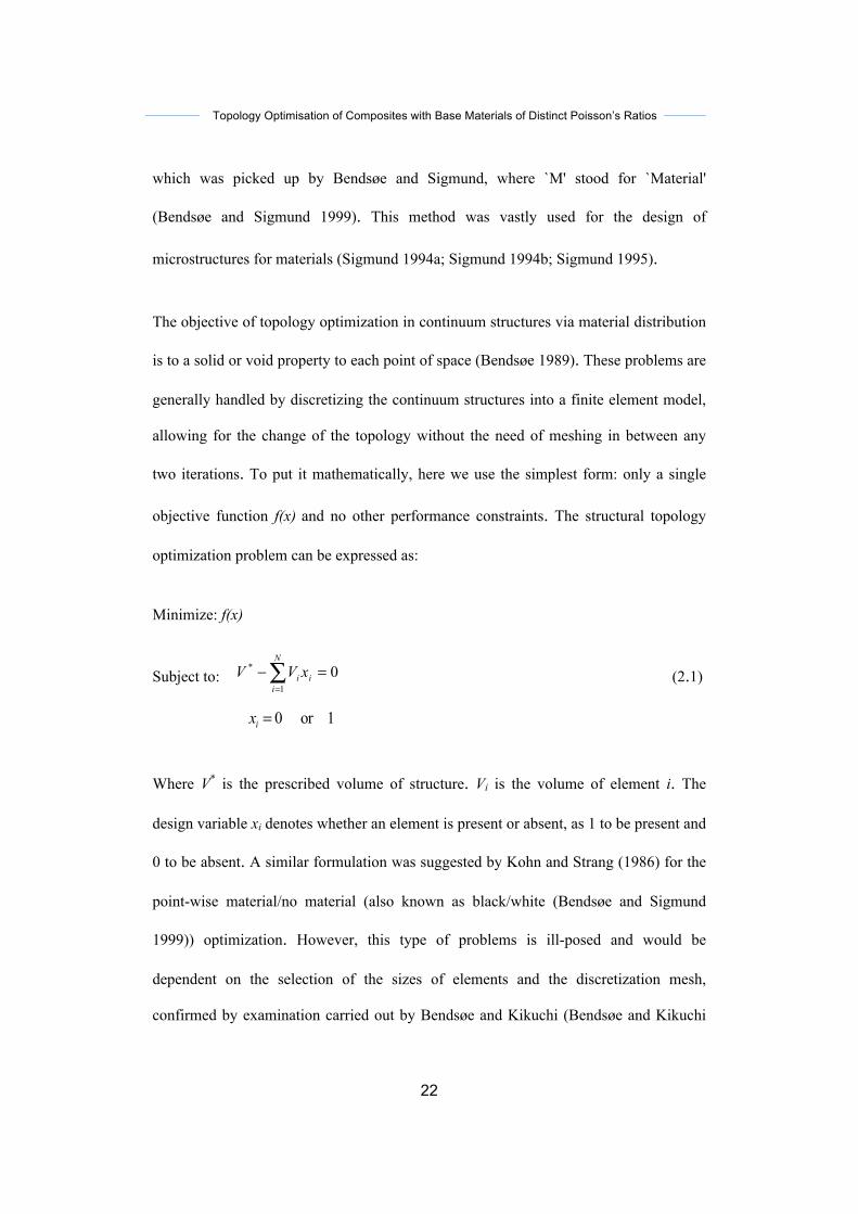
two iterations. To put it mathematically, here we use the simplest form: only a single
objective function f(x) and no other performance constraints. The structural topology
optimization problem can be expressed as:
Minimize: f(x)
(2.1) Subject to:
1or 0=ix
Where V* is the prescribed volume of structure. Vi is the volume of element i. The
design variable xi denotes whether an element is present or absent, as 1 to be present and
0 to be absent. A similar formulation was suggested by Kohn and Strang (1986) for the
point-wise material/no material (also known as black/white (Bendsøe and Sigmund
1999)) optimization. However, this type of problems is ill-posed and would be
dependent on the selection of the sizes of elements and the discretization mesh,
confirmed by examination carried out by Bendsøe and Kikuchi (Bendsøe and Kikuchi
01
* =−∑=
N
iii xVV

Topology Optimisation of Composites with Base Materials of Distinct Poisson’s Ratios
23
1988). In one example it was shown that given higher mesh density in the finite element
model of designed structure, the optimization procedure resulted in designs containing
more members of smaller sizes therefore convergence was not achievable by using even
finer mesh sizes (Bendsøe and Sigmund 1999; Huang and Xie 2010a).
The SIMP method overcomes these issues by using a relaxation method where the
design variables are freed to take any value between 0 and 1 (Sigmund and Petersson
1998) whereby some form of penalization approach then directs the solution to a
discrete value of 0 or 1. This new definition of the optimization problem can be
expressed as following:
Minimize: f(x)
(2.2)Subject to:
10 ≤≤< imin xx
where lower bound xmin is defined by density so as to avoid singularity of the
equilibrium equations. Sigmund and Petersson applied this definition to some energy
form of the structural properties (e.g. compliance). Bring back into the above equation
(2.2), it is clear that in the new formulation of the problem, the energy property was
linearly dependent on the design variable (Sigmund and Petersson 1998).
The main concern with SIMP topology optimization is in defining relationships between
materials properties (such as Young’s modulus) and the continuous design variables. To
build the link with certain material property, first we should match the design variable
01
* =−∑=
N
iii xVV
Topology Optimisation of Composites with Base Materials of Distinct Poisson’s Ratios
24
with a physical property, which procedure is also known as the interpolation scheme.
As stated previously, the design variable is often interpreted as elemental density.
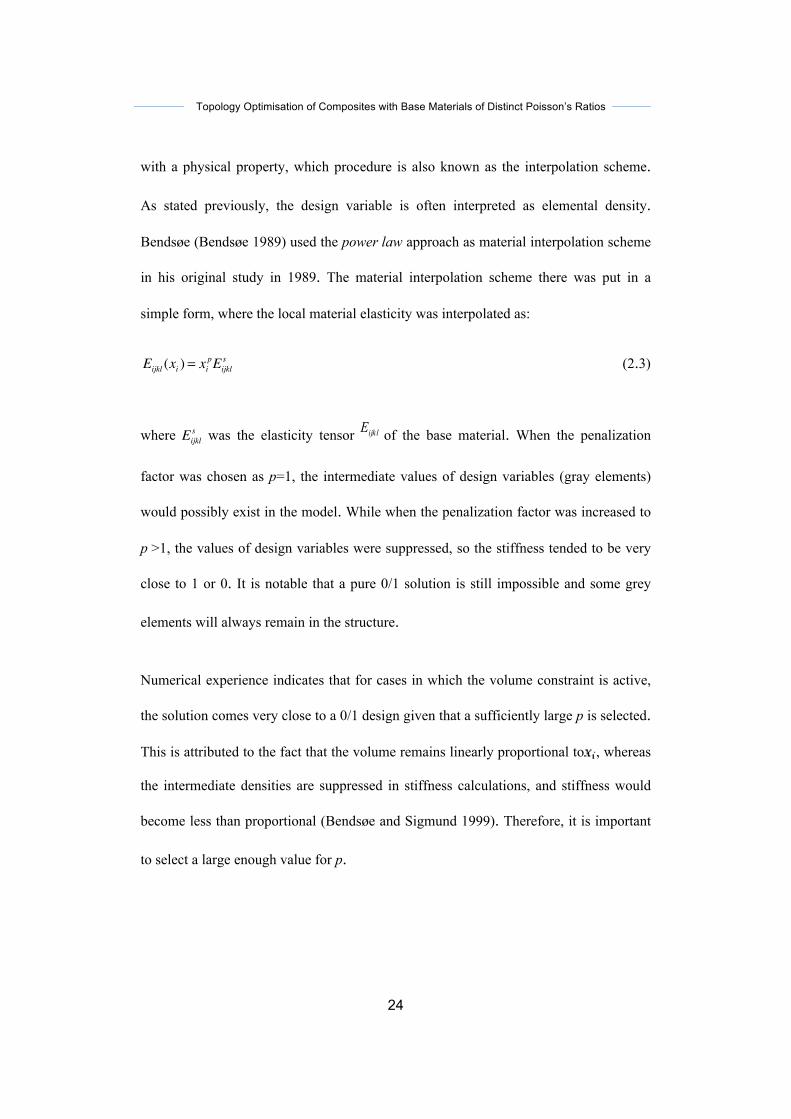
Bendsøe (Bendsøe 1989) used the power law approach as material interpolation scheme
in his original study in 1989. The material interpolation scheme there was put in a
simple form, where the local material elasticity was interpolated as:
Eijkl (xi ) = xipEijkl
s (2.3)
where Eijkls was the elasticity tensor ijklE of the base material. When the penalization
factor was chosen as p=1, the intermediate values of design variables (gray elements)
would possibly exist in the model. While when the penalization factor was increased to
p >1, the values of design variables were suppressed, so the stiffness tended to be very
close to 1 or 0. It is notable that a pure 0/1 solution is still impossible and some grey
elements will always remain in the structure.
Numerical experience indicates that for cases in which the volume constraint is active,
the solution comes very close to a 0/1 design given that a sufficiently large p is selected.
This is attributed to the fact that the volume remains linearly proportional to , whereas
the intermediate densities are suppressed in stiffness calculations, and stiffness would
become less than proportional (Bendsøe and Sigmund 1999). Therefore, it is important
to select a large enough value for p.
Topology Optimisation of Composites with Base Materials of Distinct Poisson’s Ratios
25
On the other hand, the interpolation scheme of equation (2.3) does not guarantee that
the volume distribution relationship
∑=
=N
iii xVV
1 (2.4)
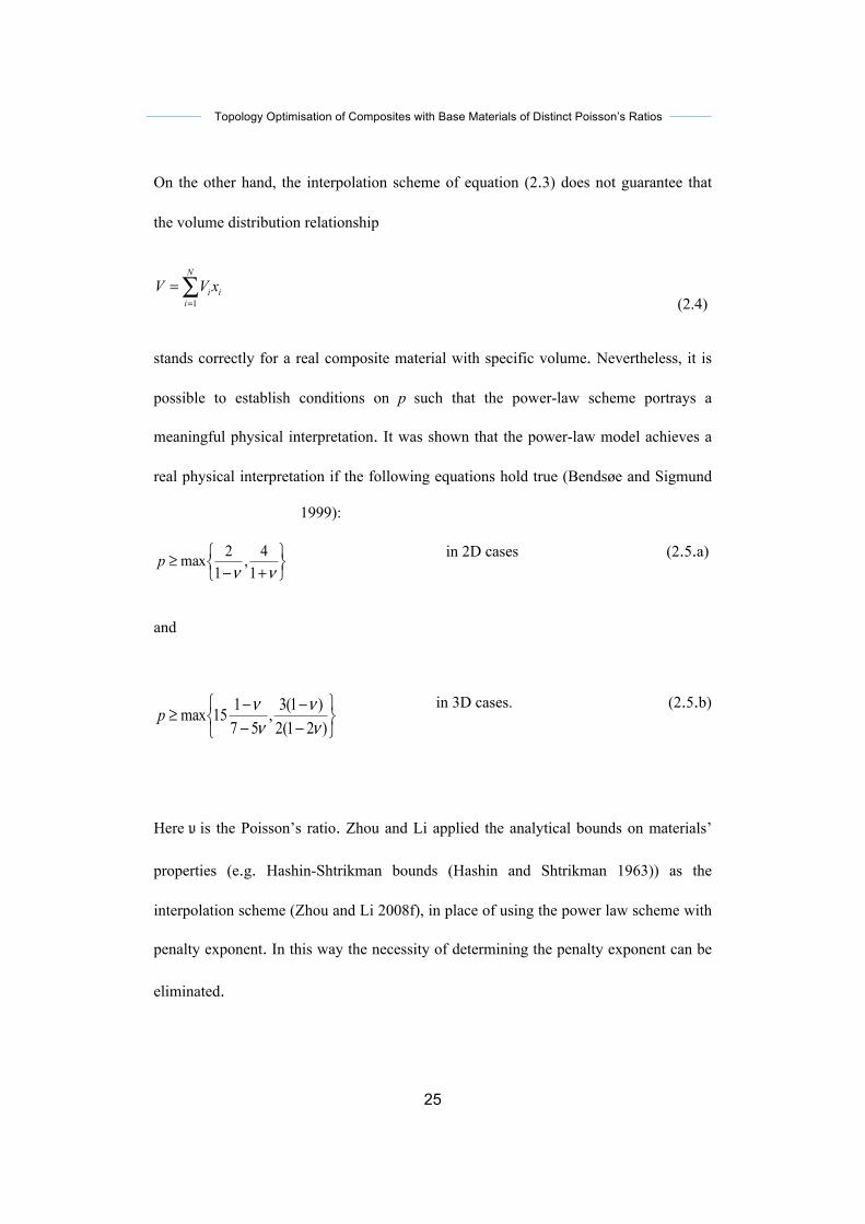
stands correctly for a real composite material with specific volume. Nevertheless, it is
possible to establish conditions on p such that the power-law scheme portrays a
meaningful physical interpretation. It was shown that the power-law model achieves a
real physical interpretation if the following equations hold true (Bendsøe and Sigmund
1999):
in 2D cases (2.5.a)
and
in 3D cases. (2.5.b)
Here is the Poisson’s ratio. Zhou and Li applied the analytical bounds on materials’
properties (e.g. Hashin-Shtrikman bounds (Hashin and Shtrikman 1963)) as the
interpolation scheme (Zhou and Li 2008f), in place of using the power law scheme with
penalty exponent. In this way the necessity of determining the penalty exponent can be
eliminated.
⎭⎬⎫
⎩⎨⎧
+−≥
νν 14,
12maxp
⎭⎬⎫
⎩⎨⎧
−−
−−≥
)21(2)1(3,
57115max
νν
ννp
Topology Optimisation of Composites with Base Materials of Distinct Poisson’s Ratios
26
A number of solution algorithms are available for structural optimization based on finite
elements (Coville 1968; Asaadi 1973; Schittkowski, Zillober et al. 1994; Chen, Silva et
al. 2001). Among them there are the “Method of Moving Asymptotes” and the “optimal
criteria methods” as two classes of numerical approaches commonly used along with
the SIMP method.
2.3 Evolutionary Structural Optimization (ESO)
A method based around the idea of gradually removing inefficient materials from the
finite element model was introduced by Xie and Steven (Xie and Steven 1993) and this
was termed the evolutionary structural optimization (ESO). The approach achieved
great acceptance due to its simplicity, leading to extensive study (Burns 2002) and
progressive development in the form of solving stiffness and displacement problems
(Chu, Xie et al. 1996), dynamic analysis of structures (Xie and G.P.Steven 1996; Zhao,
Steven et al. 1997), buckling analysis (Manickarajah, Xie et al. 1998) or multi-criteria
optimization (Proos, Steven et al. 2001). Bi-directional evolutionary structural
optimization (BESO), which was a result of studies on ESO by Querin, G.P.Steven et
al. (1998) is also considered an important development. Patil, Zhou et al. (2008)
recently employed ESO in the design of microstructures for materials to attain the
desired thermal conductivity.
Failure of a structure occurs in the event that the stress or strain at some elements
exceeds maximum values. On the other hand, low stress or strain elements can be
treated as ineffective materials. From these arguments, it can be said that identical
Topology Optimisation of Composites with Base Materials of Distinct Poisson’s Ratios
27
levels of stress should exist in every element in an ideal structure (Burns 2002). From
there, we can set the rejection criteria to be based on the stress level in elements. There
were several stress indicators taken into consideration and during the early stage of
stress-based ESO method (Xie and Steven 1993) the rejection criteria was based on von
Mises stress in elements of the structure which is an indicator of average stress in each
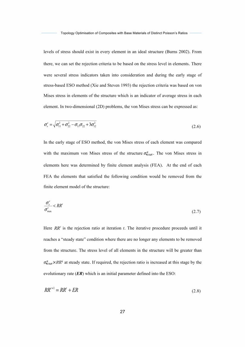
element. In two-dimensional (2D) problems, the von Mises stress can be expressed as:
2122211
222
211 3σσσσσσ +−+=ve (2.6)
In the early stage of ESO method, the von Mises stress of each element was compared
with the maximum von Mises stress of the structure . The von Mises stress in
elements here was determined by finite element analysis (FEA). At the end of each
FEA the elements that satisfied the following condition would be removed from the
finite element model of the structure:
tv
ve RR<maxσσ
(2.7)
Here tRR is the rejection ratio at iteration t. The iterative procedure proceeds until it
reaches a “steady state” condition where there are no longer any elements to be removed
from the structure. The stress level of all elements in the structure will be greater than
at steady state. If required, the rejection ratio is increased at this stage by the
evolutionary rate (ER) which is an initial parameter defined into the ESO:
ERRRRR tt +=+1 (2.8)
Topology Optimisation of Composites with Base Materials of Distinct Poisson’s Ratios
28
Following the increase, this process is repeated until a new steady state is reached. Once
the structure reaches the required stress level, the procedure is terminated; say there are
no more elements with the stress level less that 20% of the maximum stress. Still, this is
not the ideal solution and only in a limited number of cases can a fully stress structure
be achieved (Burns 2002).
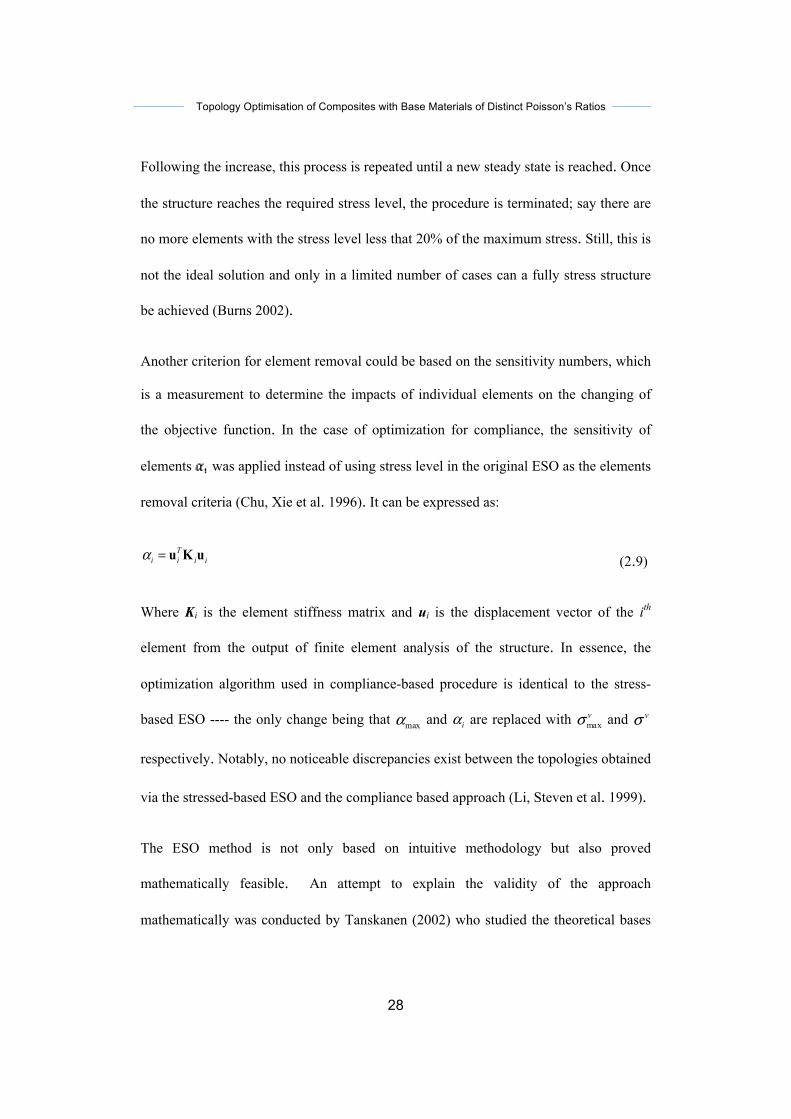
Another criterion for element removal could be based on the sensitivity numbers, which
is a measurement to determine the impacts of individual elements on the changing of
the objective function. In the case of optimization for compliance, the sensitivity of
elements was applied instead of using stress level in the original ESO as the elements
removal criteria (Chu, Xie et al. 1996). It can be expressed as:
iiTii uKu=α (2.9)
Where Ki is the element stiffness matrix and ui is the displacement vector of the ith
element from the output of finite element analysis of the structure. In essence, the
optimization algorithm used in compliance-based procedure is identical to the stress-
based ESO ---- the only change being that maxα and iα are replaced with vmaxσ and vσ
respectively. Notably, no noticeable discrepancies exist between the topologies obtained
via the stressed-based ESO and the compliance based approach (Li, Steven et al. 1999).
The ESO method is not only based on intuitive methodology but also proved
mathematically feasible. An attempt to explain the validity of the approach
mathematically was conducted by Tanskanen (2002) who studied the theoretical bases
Topology Optimisation of Composites with Base Materials of Distinct Poisson’s Ratios
29
of the compliance-based ESO. It was concluded that the ESO actually minimizes the
product of mean compliance and volume. If the design domain is modeled using equally
sized elements, the ESO was found to be similar to the sequential linear programming
method (SLP) optimization method (Tanskanen 2002).
The numerical instabilities such as checkerboard pattern and mesh dependency in the
ESO method can be avoided by developing a smoothing algorithm by averaging the
sensitivity of elements with the sensitivities of surrounding elements (Li, Steven et al.
2001). The simplicity of ESO as a topology optimization approach in both theory and
application becomes its main advantage. The approach is easily applied as a post-
processing algorithm to most finite element packages. Furthermore, the approach is
more cost-effective since the size of the finite element model is reduced as elements are
gradually removed. Besides that, the results are easier to interpret since the produced
topology is made up of a clear distinctive region, without gray areas. On the other hand,
recovery is unfeasible in the ESO approach if some elements are accidentally removed
from the structure (Zhou and Rozvany 2001). To circumvent such situations in ESO, it
is usually necessary to use very small evolutionary rates, at the expense of more costly
optimization. This means that although ESO is capable of significantly improving the
initial topology, however in some cases the results may not certainly be a global
optimum (Huang and Xie 2010; Huang and Xie 2010).
Topology Optimisation of Composites with Base Materials of Distinct Poisson’s Ratios
30
2.4 The level set method
The level-set method is a mathematical concept introduced by Osher and Sethian (1988)
for computation of moving interfaces (Burger and Osher 2005). Recently, it has been
used as a numerical alternate procedure to material distribution methods for structural
topology optimization (Sethian and Wiegmann 2000; Osher and Santosa 2001; Wang et
al. 2003), as well as being applied to an extended variety of topology optimisation
problems. These include compliance mechanics (de Gournay, Allaire et al. 2008) and
design of microstructures for materials (Mei and Wang 2004; Wilkins, Challis et al.
2007; Challis, Roberts et al. 2008). These materials include those with negative
Poisson’s ratio (Wang and Wang 2005b), specific electromagnetic characteristics
(Zhou, Li et al. 2010; Zhou, Li et al. 2011) and negative permeability (Zhou, Li et al.
2011).
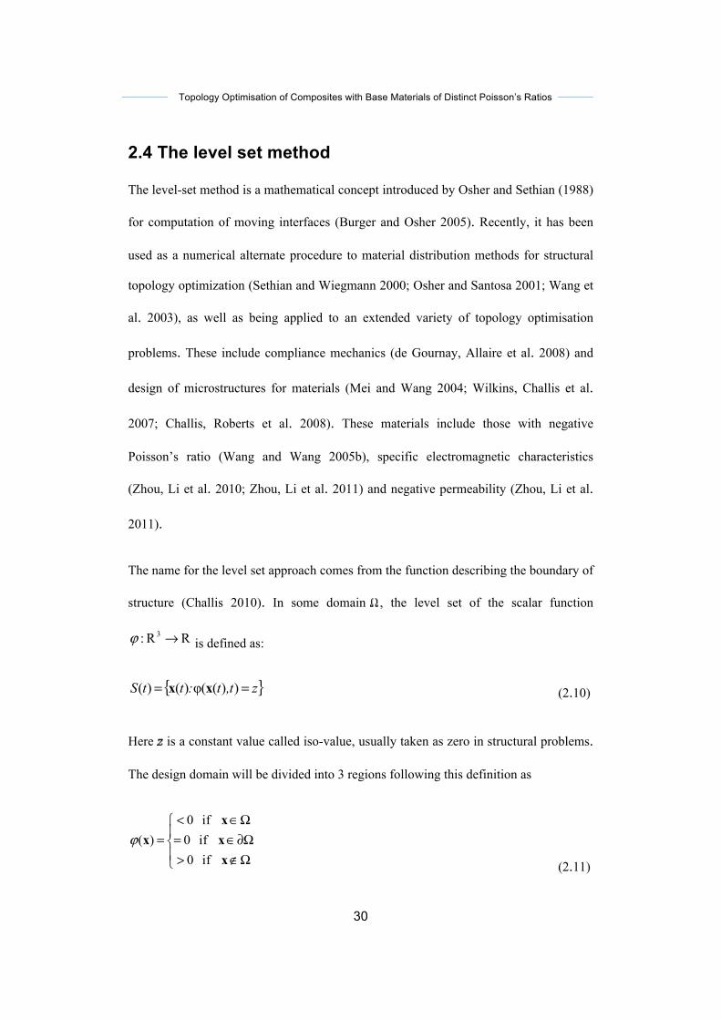
The name for the level set approach comes from the function describing the boundary of
structure (Challis 2010). In some domain , the level set of the scalar function
RR: 3 →ϕ is defined as:
{ }z,tt:ttS == ))(φ()()( xx (2.10)
Here is a constant value called iso-value, usually taken as zero in structural problems.
The design domain will be divided into 3 regions following this definition as
⎪⎩
⎪⎨⎧
Ω∉>Ω∂∈=Ω∈<
=xxx
x if 0 if 0 if 0
)(ϕ
(2.11)
Topology Optimisation of Composites with Base Materials of Distinct Poisson’s Ratios
31
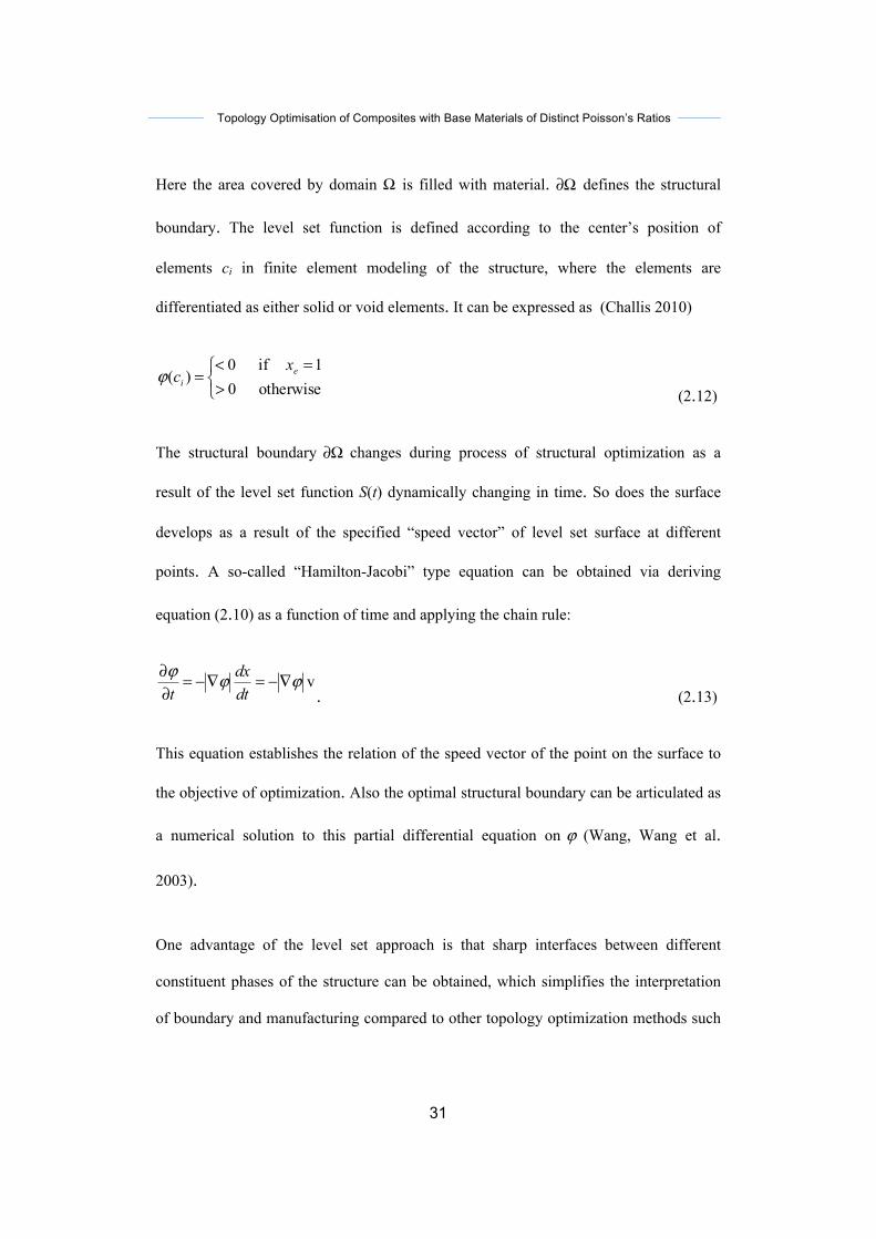
Here the area covered by domain Ω is filled with material. Ω∂ defines the structural
boundary. The level set function is defined according to the center’s position of
elements ci in finite element modeling of the structure, where the elements are
differentiated as either solid or void elements. It can be expressed as (Challis 2010)
⎩⎨⎧>
=<=
otherwise 01 if 0
)( ei
xcϕ
(2.12)
The structural boundary Ω∂ changes during process of structural optimization as a
result of the level set function S(t) dynamically changing in time. So does the surface
develops as a result of the specified “speed vector” of level set surface at different
points. A so-called “Hamilton-Jacobi” type equation can be obtained via deriving
equation (2.10) as a function of time and applying the chain rule:
vϕϕϕ ∇−=∇−=∂∂
dtdx
t . (2.13)
This equation establishes the relation of the speed vector of the point on the surface to
the objective of optimization. Also the optimal structural boundary can be articulated as
a numerical solution to this partial differential equation on ϕ (Wang, Wang et al.
2003).
One advantage of the level set approach is that sharp interfaces between different
constituent phases of the structure can be obtained, which simplifies the interpretation
of boundary and manufacturing compared to other topology optimization methods such
Topology Optimisation of Composites with Base Materials of Distinct Poisson’s Ratios
32
as SIMP, which uses continuous variables (Burger and Osher 2005). On the other hand,
the classical formulation does not allow the systematic formulation of new holes in the
topology of structure, especially in two-dimensional cases (Allaire, Jouve et al. 2004).
As the level set method generally describes the propagation of interfaces with a defined
speed function, holes within existing shapes and away from the boundaries cannot be
initiated (Burger, Hackl et al. 2004).
Various solutions were proposed to overcome problems relating to the nucleation of
new holes in the structure. A large number of discrete holes could be introduced in the
initial design (Allaire, Jouve et al. 2004). The above-mentioned level set setting is
capable of merging or cancelling these holes and creating a structure with fewer holes in
following iterations. Still the level set method is not capable of creation of further holes
during the optimization process, but only in initial stage. This is the reason why the
number and location of the initial holes largely influence the final solution (Wang,
Wang et al. 2003; Allaire, Jouve et al. 2004).
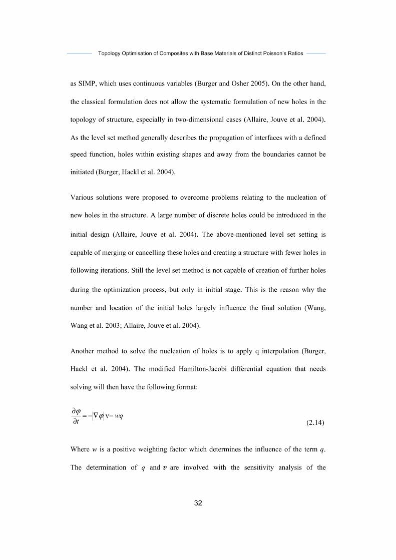
Another method to solve the nucleation of holes is to apply q interpolation (Burger,
Hackl et al. 2004). The modified Hamilton-Jacobi differential equation that needs
solving will then have the following format:
wqt
−∇−=∂∂ vϕϕ
(2.14)
Where w is a positive weighting factor which determines the influence of the term q.
The determination of q and are involved with the sensitivity analysis of the
Topology Optimisation of Composites with Base Materials of Distinct Poisson’s Ratios
33
optimization objective function. The selected q is dependent on the problem at hand and
its weighting factor should be determined by the user as an initial parameter (Challis
2010) and therefore its successful application is highly dependent on previous
experiences. The introduction of additional constraints in the level set approach
involves further modification into the Hamilton-Jacobi differential equation (2.14)
through addition of extra weighted terms (Challis, Roberts et al. 2008). Thus,
successfully implanting the method in conjunction with extra constraints becomes
cumbersome in two-dimensional problems.
Generally, the level set approach is considered to be more mathematically complicated
and difficult to implement as a computational procedure, in contrast to materials
distribution approaches, the SIMP, ESO and BESO. This has prevented it from regular
application (Rozvany 2009). As for materials distribution approaches, due to their
mathematical simplicity, these methods have received greater attention besides being
more developed.
2.5 Bi-Directional Evolutionary Structural Optimization (BESO) The bi-directional evolutionary structural optimization (BESO) method was the next
generation product based on its 1.0 version of the evolutionary structural optimization
(ESO) method. Research on this area has been very active and extensive with many
algorithms proposed within the past fifteen years since the term “BESO” was first
introduced (Querin 1997; Querin et al. 1998). The various versions of former BESO
methods attempted to solve shape/topology optimization problems empirically and have
Topology Optimisation of Composites with Base Materials of Distinct Poisson’s Ratios
34
been unsuccessful in guaranteeing optima in the solutions (Rozvany 2001). Recently, an
advanced BESO approach which yields mesh-independent and convergent solutions
was proposed by Huang and Xie (2007). This was followed by proposal of a
mathematically established formulation for this BESO (Huang and Xie 2009) which
solves the stiffness optimization problem using soft-kill approach (i.e. replacing void
elements with soft material) that is shown to be equivalent to hard-kill (complete
removal of elements designated as void). Final optima can be ensured in this advanced
version of BESO by incorporating a more rigorous optimality criterion.
An overview of the BESO method is presented in following session with basic concepts
of the BESO method explained and formulations devised for the most simple and basic
situation which is periodic optimal design under given ratio with one single base
material.
Although in BESO method the most obvious advance than ESO is that it’s capable to
re-admit elements into the design domain, in previous versions (Querin 1997; Querin et
al. 1998; Yang et al. 1999; Zhu et al. 2007) it was still not capable of ensuring optima
(Rozvany 2001; Zhou and Rozvany 2001; Rozvany 2008). This was due to a number of
reasons from various aspects. Initially, the assumption of sensitivities for void elements
was not accurate which further more delivered inaccurate estimation on the change of
the optimization objective. In some previous versions, void elements around high-
performance solid elements were subject to heuristic re-admission, owing to insufficient
information on the absent elements. Also, non-convergence prevents the production of
reliable results. This shortcoming requires one to pick out the best solution among
Topology Optimisation of Composites with Base Materials of Distinct Poisson’s Ratios
35
several possible ones which can be very difficult and lose the point of optimization. At
last there is neither direct mathematical explanation for the approach nor indirect
demonstration to confirm that the design evolves towards an optimum. So as a result the
removal or admission of elements is quite intuitive driven.
Moreover, an essential feature expected from most of the popular topology optimization
techniques is mesh-independence. Mesh-dependence is considered a numerical
instability (Sigmund and Peterson 1998; Bendsøe and Sigmund 2003), which leads to
the occurrence of dense holes in the final design, usually called the checkerboard
pattern. These make further detailed designs unfeasible. Attempts to overcome this have
been made using algorithms such as perimeter control (Yang et al. 2003) and a
smoothing algorithm (Li et al. 2001). The filter scheme developed by Huang and Xie
(Huang and Xie 2007) is used in this present work. The filter scheme is able suppress
the checker-board patterns and work for mesh-independence, besides also acting as an
effective mechanism for extrapolating sensitivity numbers from solid elements to void
elements.
An improved and mathematically based BESO approach was proposed by Huang and
Xie (Huang and Xie 2007; Huang and Xie 2009) to overcome the difficulties described
above. In this improved BESO version, soft-kill of elements is applied instead of hard-
kill, which means when a solid element is replaced, it would be by soft element rather
than void element. The filter scheme makes up one of the basic algorithms in this new
version, which is able to guarantee final optima by applying such rigorous optimality
criteria. This improved BESO method has been applied to a variety of stiffness
Topology Optimisation of Composites with Base Materials of Distinct Poisson’s Ratios
36
optimization problems and proven to be capable to achieve mesh-independent and
convergent design results.
2.5.1. Hard-kill BESO
Following the ESO method which based on the idea of gradually removing inefficient
elements off from the finite element model of the structure, the method called “additive
evolutionary structural optimization” (AESO) has been introduced targeting generating
optimum structures with initial design of a minimum ground structure and gradually
adding elements to it (Querin, G.P.Steven et al. 1998; Querin, Steven et al. 2000). In
the AESO method, new elements would be added to the free edges of the most efficient
elements where the most efficient elements are selected by the standard of elements
with highest stress or sensitivity numbers (Querin, Steven et al. 2000). BESO, another
member in the ESO method family tree and yet the most developed one, was created
along the trend with added flexibility and stableness (Yang, Xie et al. 1999). In BESO
method elements can be added and/or removed in each iteration. The criteria for adding
or removing of elements are based on their effects on variation of objective functions.
The numbers of added or removed elements are controlled by two given parameters, the
inclusion ratio (IR) and rejection ratio (RR) respectively.
As mentioned before sensitivity numbers expresses such effects. In a classic BESO
project, the sensitivity numbers are calculated according to the results of structural
analysis for solid elements. While for void elements the sensitivity numbers are
calculated based on their nodal displacements, which are calculated by extrapolating the
nodal displacements of their surrounding solid elements. The method takes after
Topology Optimisation of Composites with Base Materials of Distinct Poisson’s Ratios
37
primarily by the ranking of elements in view of the extent of their sensitivities. An
element will be changing to solid if it is with higher sensitivities, or to void for those
who have lower sensitivity numbers. Like soft-kill BESO method, the quantities of
removed and added elements are treated with two separate criteria by adding a
constraint of volume-fraction changing ratio between two adjacent iterations.
The urge for an improved optimization method had been raised due to dissatisfaction of
earlier solutions. As mentioned earlier, the proposed optimization problem of solid-void
material distribution could not reach a universal solution because the elements sizes and
discretization meshes fatally influences this supposed optimization problem as
demonstrated by Bendsøe and Kikuchi (Bendsøe and Kikuchi 1988). Other
disadvantages of these earlier methods include that the numerical instability was not
handled well as well as computational efficiency was relatively low due to the
convergence problems (Rozvany 2009; Huang and Xie 2010a). Furthermore we need to
list out all possible topologies that are generated via various RR and IR in order to find
out the final best solution (Rozvany 2009; Huang and Xie 2010a).
Huang and Xie (Huang and Xie 2007) developed a new algorithm for the hard-kill
BESO in 2007. In this version they addressed several issues including a clearer
statement of the optimization problem and better solution against numerical instability
during the procedure (Huang and Xie 2010). Here it was supposed that the purpose of
the optimization was to find the stiffest structure with volume as additional constraint.
In this version of hard-kill BESO method, the optimization problem is stated as:
Topology Optimisation of Composites with Base Materials of Distinct Poisson’s Ratios
38
Minimize: f(x)=K (2.15.a)
Subject to: 0
1
* =−∑=
N
iii xVV
(2.15.b)
1or 0=ix . (2.15.c)
Here the xi is a design variable which indicates the absence or presence of an element in
the PBC, as 1 to be present and 0 to be absent. This show in BESO method an element
is considered as the smallest unit and could only be 1 or 0, in contrast to the design
variable xi in SIMP approach which is between 0 and 1.
In order to estimate the sensitivity numbers of void elements, Huang and Xie developed
a filtering scheme based on the following weighting equation (Huang and Xie 2007):
∑
∑
=
== N
jij
N
j
niij
i
w
αwα
1
1ˆ
(2.16)
In the above equation N stands for the total number of finite elements in current design
iα model and is the calculated sensitivity number of element i. The weight factor ijw is
expressed as:
⎩⎨⎧ <−
=otherwise 0
if minmin rrrrw ijijij
(2.17)
Here rij states the distance between the centres of element i and that of element j. The
filter radius rmin defines till how far a neighbouring element could have an impact on the
Topology Optimisation of Composites with Base Materials of Distinct Poisson’s Ratios
39
sensitivity of element i. Initially the sensitivity numbers of void elements were
temporarily assumed at zero, which would then be modified near the end of each
iteration through out the optimisation process according to the filtering scheme.
It would be followed by adding and removing of elements, both of which are based on
the rank of each element among all elements in the PBC. Those elements that have
lower sensitivity numbers would be switched to void elements; whereas for those
elements those have higher sensitivity numbers they would be designated to solid
elements instead. In a word, the filtering scheme is to rank each element by a number
calculated from its own sensitivity number and weight factors of surrounding elements
(Huang and Xie 2010).
The numerical instabilities in the original versions (Zhou and Rozvany 2001; Rozvany
2009) caused quite a few controversies. But by introducing the filtering scheme
described above (Huang and Xie 2010), more successful optimisations were archived
with less occurrence of so-said instabilities. With that being said, another significant
improvement made by Huang and Xie (Huang and Xie 2010) is the unified criteria for
adding and removing of elements. Volumetric constraint can then be carried out exactly
as a parameter by applying the criteria. Furthermore, this revised hard-kill BESO
method has much higher computational efficiency besides above-mentioned
improvements. It is as well for the reason that the removed elements would not be
engaged in following FEA, hence less elements to be considered better the time
consumption of the FEA (Huang and Xie 2010).

Topology Optimisation of Composites with Base Materials of Distinct Poisson’s Ratios
40
2.5.2. Soft-kill BESO
Rozvany pointed out that solid elements could only grow around or nearby existing
solid elements by applying above introduced Hard-kill BESO method (Rozvany 2001).
In some cases that may induce to failure in correcting the incorrect element rejection
(Zhou and Rozvany 2001; Zhu, Zhang et al. 2007). Besides that point, other findings
also specified that complete removal of void elements might also cause certain
dilemma, especially for multi-phase cases (Sigmund 2001; Zhu, Zhang et al. 2007;
Huang and Xie 2010a).
In attempt to solve these problems, Hinton and Sienz (Hinton and Sienz 1995) tested
another substitute approach based on ESO where the design domain is fully stressed and
pointing material properties to elements is bi-directional. Here bi-directional means
rather than complete removal of void elements a comparatively small density can be
assigned to the void elements, which is assumed possessing 106 times lower elastic
modulus than solid elements (Hinton and Sienz 1995). The bi-directional method allows
void elements to carry a stain value to stay in FEA hence they might be assigned as
solid elements along the optimisation process. In other words solid elements can grow
in any desired region of the structure instead of limited to around existing solid regions
(Rozvany 2001; Zhu, Zhang et al. 2007).
It’s worth mentioning another BESO method developed by Zhu, Zhang et al. (Zhu,
Zhang et al. 2007), which is sensitivity based. The innovation highlighted in this
method is to use orthotropic cellular microstructure (OCM) in place of void elements,

Topology Optimisation of Composites with Base Materials of Distinct Poisson’s Ratios
41
i.e. according to their sensitivity rankings elements would be assigned as OCM’s or
solid elements respectively. Here the OCM is defined as a microstructural system with
very low density. A filter scheme is applied to avoid numerical instability, which
controls the array of continued solid elements along each principal direction (Zhu,
Zhang et al. 2007). Though improvements have been made based on hard-kill BESO
nevertheless both methods experience some problems on convergence (Huang and Xie
2010).
It was until 2009 Huang and Xie published the soft-kill BESO method that the above-
mentioned hard-kill BESO limits were conquered. In this soft-kill BESO method when
an associated element is void, the design variable xi would be assigned to a relatively
small value xmin (e.g. 0.001), so as to keep such elements involved in continuing FEA
(Huang and Xie 2009). The optimisation problem here can be stated as
Minimize: f(x)=K (2.18.a)
Subject to: 0
1
* =−∑=
N
iii xVV
(2.18.b)
1or mini xx = (2.18.c)
The most common application is in stiffness optimisation where the sensitivity of
elements is based on the objective function f(x) with respect to design xi variable. Use
the case of Young’s modulus as effective property in stiffness optimisation as an

Topology Optimisation of Composites with Base Materials of Distinct Poisson’s Ratios
42
example. The objective function here is a function of the effective Young’s modulus of
PBC, which can be expressed though a power-law interpolation scheme (Bendsøe 1989)
pis xEE )(i )(x = (2.19)
Here E(s) stands for the Young’s modulus of the solid material. p is a penalty exponent
assigned manually. There is a similarity of results observed between this soft-kill BESO
method and the hard-kill one (Huang and Xie 2007, Huang and Xie 2010). As stated by
Huang and Xie (Huang and Xie 2010a), the sensitivity numbers of soft elements are
dependent on penalty exponent p. When p approaches infinity, the sensitivity numbers
of solid elements and “void” elements would become the elemental strain energy and
zero respectively, same as that of the hard-kill BESO method. Such consistency also
happens to the objective function. Hence the hard-kill BESO method can be seen as a
special case of the soft-kill BESO method with penalty exponent p→∞.
Topology Optimisation of Composites with Base Materials of Distinct Poisson’s Ratios
43
Chapter3TopologyoptimizationofCompositesforMaximisingEffectiveYoung'sModuli
In the case of composites design for optimal stiffness, the effective Young’s modulus
and Poisson’s ratio of the composite material are obtained through homogenization
theory. Single or multiple objectives are defined to maximize these properties separately
Topology Optimisation of Composites with Base Materials of Distinct Poisson’s Ratios
44
or in combination. Based on the sensitivity analysis of the objective function, a BESO
calculation is conducted to achieve optimized topology for the composite unit cell.
This chapter investigates the effect of Poisson’s ratio on composite materials. The study
is focused on composites containing two materials with different Poisson’s ratios,
especially when one of them is nearly incompressible, to reveal the role that Poisson’s
ratio plays in optimized composites. Two types of problems are used: maximizing E3
(where E1=E2) or maximizing E1, E2, and E3 together (where E1=E2=E3). The composite
is modelled as a microstructure in a periodic unit cell. A combined objective function is
defined in terms of the largest Young’s modulus of the composite. The overall
optimization in this study is based on the bi-directional evolutionary structural
optimization (BESO) method.
Several research questions to be answered, as follow:
1) Is it possible to build a composite with higher Young’s moduli than its base
materials? How much higher can we achieve?
2) How to develop a Fortran code for this composites optimization?
3) Is it possible to find the best volume fraction automatically?
4) What is the suitable interpolation scheme and initial design?
Topology Optimisation of Composites with Base Materials of Distinct Poisson’s Ratios
45
5) When expanding the range of Poisson’s ratio to (-1, 0), will this program be
applicable? And how will the negative Poisson’s ratio affect the optimization
procedure and results?
6) Is there any limitation for this method to be applicable and why?
3.1. Methodology
3.1.1 Optimization problem statement
The optimisation problem can be stated as follows:
Maximize:)(
31
321 EEEf ++=, (3.1a)
Subject to:0
1
* =−∑=
N
eee xVV
,
minxxe = or 1, (3.1b)
Where E1, E2 and E3 are the effective Young’s moduli of the composite. Equation (3.1a)
stated that all the three effective moduli are to be maximized. Alternatively, one can
choose to maximize a single modulus, that is
Maximize: f =E3. (3.2)

Topology Optimisation of Composites with Base Materials of Distinct Poisson’s Ratios
46
3.1.2 Optimization with optimum volume to be solved
In BESO, the above problems are solved by iteratively searching the optimum
according to the element sensitivity, denoted as αε. For problem as defined in Eq. 2, the
optimum volume is estimated at each iteration according to the element sensitivity. The
problem statement of this case can be generally stated as ‘to find the value of x (volume)
at which the function f(x) has its maximum. When f(x) is the bulk modulus K, the
solution is simple, that is x =1 and f(x)=K2. When f(x) is E as in this case, x is to be
solved by incorporating an addition algorithm in BESO.
The methodology is as follows. The volume target is estimated at each iteration
according to the element sensitivity. Assume that the topology has totally NE element,
and at iteration i, the number of element of materials 1 and 2 are NE1 and NE2,
respectively.
Check the element sensitivity eα , and
l Sum up the number of elements of material 2 which has 0<eα , denoted as −2NE .
l Sum up the number of elements of material 1 which has 0>eα , denoted as +1NE .
Then the target volume is calculated as
NENENENEVt
+− +−= 122
(3.3)
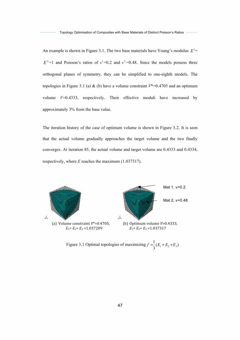
Topology Optimisation of Composites with Base Materials of Distinct Poisson’s Ratios
47
An example is shown in Figure 3.1. The two base materials have Young’s modulus 1E =
2E =1 and Poisson’s ratios of 1v =0.2 and 2v =0.48. Since the models possess three
orthogonal planes of symmetry, they can be simplified to one-eighth models. The
topologies in Figure 3.1 (a) & (b) have a volume constraint V*=0.4705 and an optimum
volume V=0.4333, respectively. Their effective moduli have increased by
approximately 3% from the base value.
The iteration history of the case of optimum volume is shown in Figure 3.2. It is seen
that the actual volume gradually approaches the target volume and the two finally
converges. At iteration 85, the actual volume and target volume are 0.4333 and 0.4334,
respectively, where E reaches the maximum (1.037317).
(a) VolumeconstraintV*=0.4705,
E1=E2=E3=1.037209
(b) OptimumvolumeV=0.4333,
E1=E2=E3=1.037317
Figure 3.1 Optimal topologies of maximizing )(31
321 EEEf ++=
Mat 1, v=0.2
Mat 2, v=0.48

Topology Optimisation of Composites with Base Materials of Distinct Poisson’s Ratios
48
0.0
0.2
0.4
0.6
0.8
1.0
1.000
1.005
1.010
1.015
1.020
1.025
1.030
1.035
1.040
0 20 40 60 80 100
Vol
ume
V
Stif
fnes
s E
Iteration History
E
Target volume
Actual volume
Figure 3.2 Iteration histories of effective modulus and optimum volume
3.1.3 Verification on sensitivity analysis
One essential procedure of the BESO algorithm is to calculate the element sensitivity.
This part is to verify that for problems dealing with different Poisson’s ratio, such
calculation is conducted correctly in the BESO code.
There are three aspects in the calculation, i.e.
a) Assumption of interpolation function.
b) Implementing the equation of sensitivity.
c) Implementing the filter procedure.
They are investigated/verified as follows (reversely ordered).
c) Verification of filter procedure
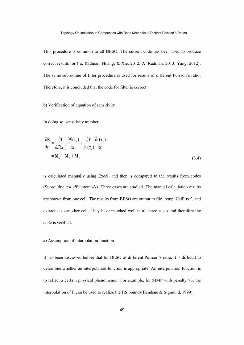
Topology Optimisation of Composites with Base Materials of Distinct Poisson’s Ratios
49
This procedure is common to all BESO. The current code has been used to produce
correct results for ( a. Radman, Huang, & Xie, 2012; A. Radman, 2013; Yang, 2012).
The same subroutine of filter procedure is used for results of different Poisson’s ratio.
Therefore, it is concluded that the code for filter is correct.
b) Verification of equation of sensitivity
In doing so, sensitivity number
cba
e
e
ee
e
ee xxv
xvxxE
xEx
MMM
EEE
++=
∂∂
∂∂+
∂∂
∂∂=
∂∂ )(
)()(
)(
(3.4)
is calculated manually using Excel, and then is compared to the results from codes
(Subroutine cal_dEmatrix_dx). Three cases are studied. The manual calculation results
are shown from one cell. The results from BESO are output to file ‘temp_CalE.txt’, and
extracted to another cell. They have matched well in all three cases and therefore the
code is verified.
a) Assumption of interpolation function
It has been discussed before that for BESO of different Poisson’s ratio, it is difficult to
determine whether an interpolation function is appropriate. An interpolation function is
to reflect a certain physical phenomenon. For example, for SIMP with penalty >3, the
interpolation of E can be used to realize the HS bounds(Bendsùe & Sigmund, 1999).
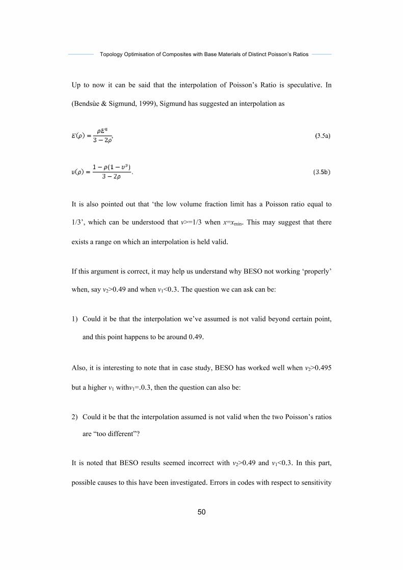
Topology Optimisation of Composites with Base Materials of Distinct Poisson’s Ratios
50
Up to now it can be said that the interpolation of Poisson’s Ratio is speculative. In
(Bendsùe & Sigmund, 1999), Sigmund has suggested an interpolation as
It is also pointed out that ‘the low volume fraction limit has a Poisson ratio equal to
1/3’, which can be understood that v>=1/3 when x=xmin. This may suggest that there
exists a range on which an interpolation is held valid.
If this argument is correct, it may help us understand why BESO not working ‘properly’
when, say v2>0.49 and when v1<0.3. The question we can ask can be:
1) Could it be that the interpolation we’ve assumed is not valid beyond certain point,
and this point happens to be around 0.49.
Also, it is interesting to note that in case study, BESO has worked well when v2>0.495
but a higher v1 withv1=.0.3, then the question can also be:
2) Could it be that the interpolation assumed is not valid when the two Poisson’s ratios
are “too different”?
It is noted that BESO results seemed incorrect with v2>0.49 and v1<0.3. In this part,
possible causes to this have been investigated. Errors in codes with respect to sensitivity

Topology Optimisation of Composites with Base Materials of Distinct Poisson’s Ratios
51
analysis have been ruled out. One other possible cause is the choice of interpolation
function. It is likely that although hard to be quantified, an interpolation function may
be only valid within a certain range.
3.1.4 Compare material interpolation schemes
Two material interpolation schemes are proposed, i.e.
1) Interpolate the E matrix
21)1( EEE pe
pe xx +−= (3.6)
2) Interpolate the E and v respectively
21)1()( ExExxE EE pe
pee +−= (3.7a)
21)1()( vxvxxv vv pe
pee +−= (3.7b)
For using E matrix interpolation, it is noticed that the topology changes rather random
between iterations. This may suggest that the searching is not in the right path. Changin
g the interpolation from E matrix to E and v interpolation, the change between iterations
becomes gradual, and reasonable results are obtained.
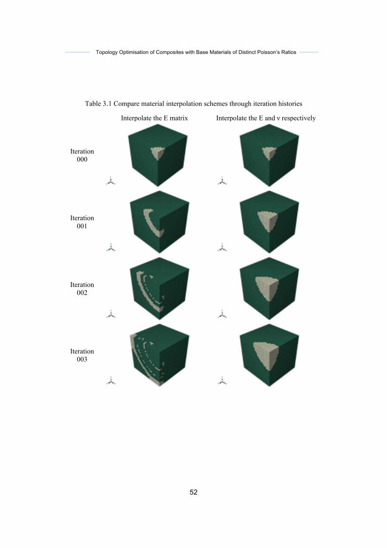
Topology Optimisation of Composites with Base Materials of Distinct Poisson’s Ratios
52
Table 3.1 Compare material interpolation schemes through iteration histories
Interpolate the E matrix Interpolate the E and ν respectively
Iteration 000
Iteration 001
Iteration 002
Iteration 003

Topology Optimisation of Composites with Base Materials of Distinct Poisson’s Ratios
53
Another two interpolation schemes are investigated as well, i.e.
1) SIMPinterpolation:
E(xe ) = E2xe
p + E1(1− xe
p ) (3.8)
2) Qinterpolation:
E(xe ) = E1 +xe(E2 − E1)1+ q(1− xe )
(3.9)
When both base materials possess positive Poisson’s ratio and maximizing E3:
penalty=1 got highest E3 and comparably lower E1 and E2; compare SIMP and Q
interpolation, SIMP interpolation focus better on E3 maximization. In future studies,
SIMP interpolation with penalty p=1 will be used when maximizing E3 (where E1=E2).
The topology presents a constant pattern of base material 2 re-distributed along the
strongest axis while the overall stiffness is optimized. It was noticed that case study on
v2=0.49 ended up with incorrect result. The current method is not compatible when
v2≥0.49.
Table 3.2 Base materials ---- Eb1=1, v1=0.1, Eb2=1, v2=0.48
Interpolation Penalty Optimum
volume E1 E2 E3 Topology
Q 1 0.4941 1.04268 1.04268 1.11017 (a)
Q 2 0.4919 1.05242 1.05242 1.09311 (b)
Q 3 0.4831 1.05950 1.05950 1.08175 (c)
SIMP 1 0.4269 1.04096 1.04096 1.11545 (d)
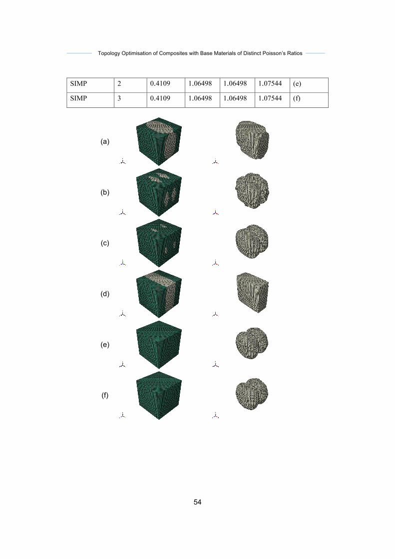
Topology Optimisation of Composites with Base Materials of Distinct Poisson’s Ratios
54
SIMP 2 0.4109 1.06498 1.06498 1.07544 (e)
SIMP 3 0.4109 1.06498 1.06498 1.07544 (f)
(a)
(b)
(c)
(d)
(e)
(f)
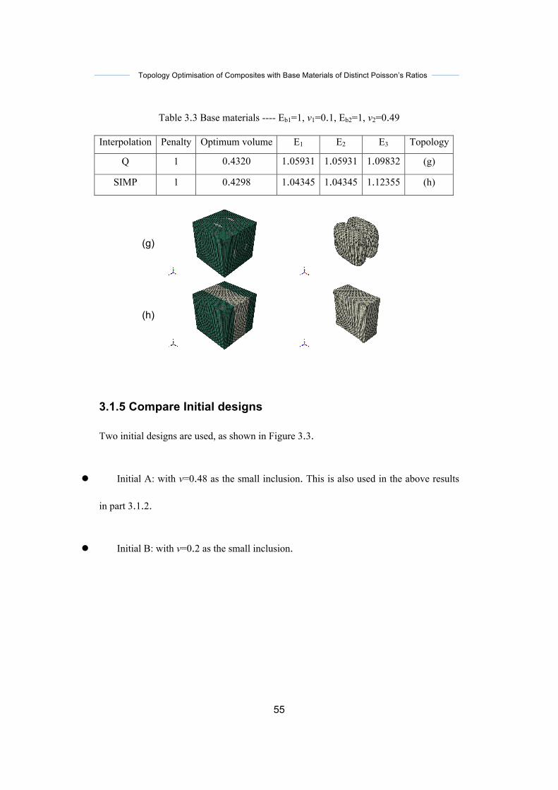
Topology Optimisation of Composites with Base Materials of Distinct Poisson’s Ratios
55
Table 3.3 Base materials ---- Eb1=1, v1=0.1, Eb2=1, v2=0.49
Interpolation Penalty Optimum volume E1 E2 E3 Topology
Q 1 0.4320 1.05931 1.05931 1.09832 (g)
SIMP 1 0.4298 1.04345 1.04345 1.12355 (h)
(g)
(h)
3.1.5 Compare Initial designs
Two initial designs are used, as shown in Figure 3.3.
l Initial A: with v=0.48 as the small inclusion. This is also used in the above results
in part 3.1.2.
l Initial B: with v=0.2 as the small inclusion.
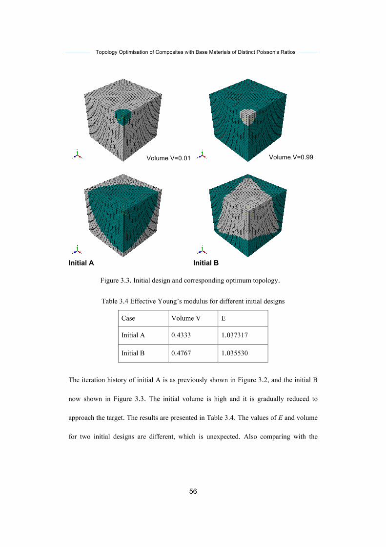
Topology Optimisation of Composites with Base Materials of Distinct Poisson’s Ratios
56
Initial A Initial B
Figure 3.3. Initial design and corresponding optimum topology.
Table 3.4 Effective Young’s modulus for different initial designs
Case Volume V E
Initial A 0.4333 1.037317
Initial B 0.4767 1.035530
The iteration history of initial A is as previously shown in Figure 3.2, and the initial B
now shown in Figure 3.3. The initial volume is high and it is gradually reduced to
approach the target. The results are presented in Table 3.4. The values of E and volume
for two initial designs are different, which is unexpected. Also comparing with the
Volume V=0.01 Volume V=0.99

Topology Optimisation of Composites with Base Materials of Distinct Poisson’s Ratios
57
previous cases, E value of Initial B is lower. This may suggest that the result is
incorrect.
Figure 3.4. Iteration history for initial design B
Here examine the possible explanation for the low value. Combine the iteration history
for initial A (Figure 3.2) and initial B (Figure 3.4). Now use the volume instead of
iteration as the x- axis. Initial A starts from the lower volume and initial B starts from
high volume. There is a gap between the two respective maximum points. How the
optimum E changes between the gaps is questionable. One possibility is that it may
have some local peaks, as sketched in the close-up of the circled area. After Initial B
reaches the local peak B, the search will terminate and be unable to follow the drop
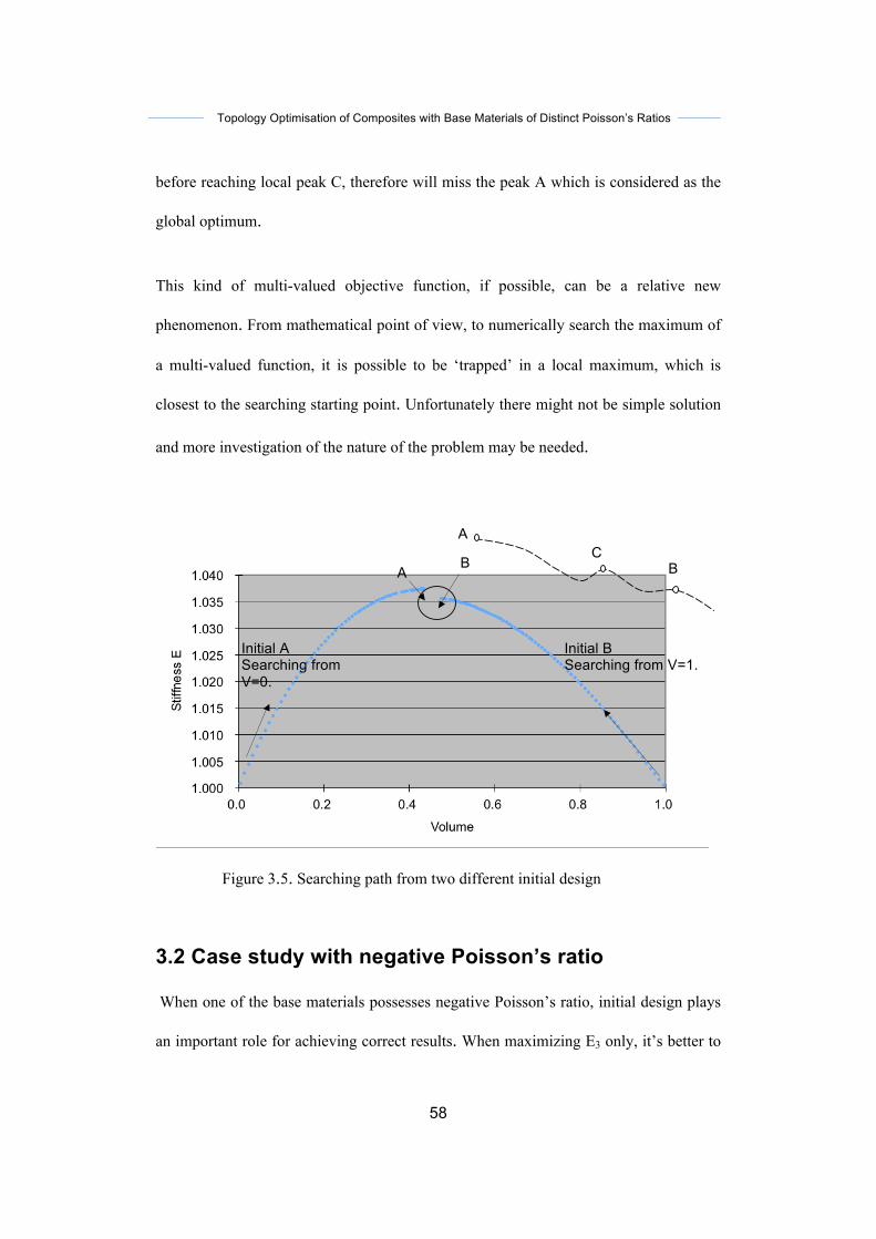
Topology Optimisation of Composites with Base Materials of Distinct Poisson’s Ratios
58
before reaching local peak C, therefore will miss the peak A which is considered as the
global optimum.
This kind of multi-valued objective function, if possible, can be a relative new
phenomenon. From mathematical point of view, to numerically search the maximum of
a multi-valued function, it is possible to be ‘trapped’ in a local maximum, which is
closest to the searching starting point. Unfortunately there might not be simple solution
and more investigation of the nature of the problem may be needed.
Figure 3.5. Searching path from two different initial design
3.2 Case study with negative Poisson’s ratio
When one of the base materials possesses negative Poisson’s ratio, initial design plays
an important role for achieving correct results. When maximizing E3 only, it’s better to
A B
Initial B Searching from V=1.
Initial A Searching from V=0.
A
B C
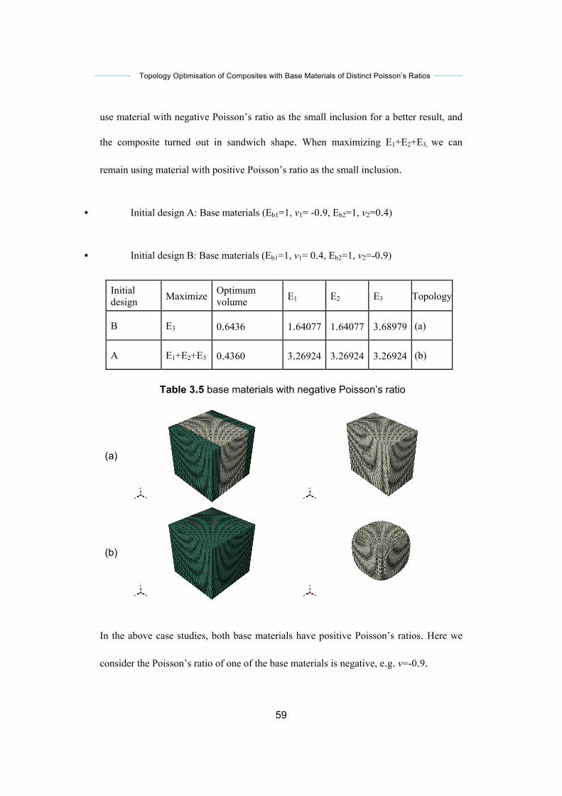
Topology Optimisation of Composites with Base Materials of Distinct Poisson’s Ratios
59
use material with negative Poisson’s ratio as the small inclusion for a better result, and
the composite turned out in sandwich shape. When maximizing E1+E2+E3, we can
remain using material with positive Poisson’s ratio as the small inclusion.
• Initial design A: Base materials (Eb1=1, v1= -0.9, Eb2=1, v2=0.4)
• Initial design B: Base materials (Eb1=1, v1= 0.4, Eb2=1, v2=-0.9)
Table 3.5 base materials with negative Poisson’s ratio
(a)
(b)
In the above case studies, both base materials have positive Poisson’s ratios. Here we
consider the Poisson’s ratio of one of the base materials is negative, e.g. v=-0.9.
Initial design Maximize Optimum
volume E1 E2 E3 Topology
B E3 0.6436 1.64077 1.64077 3.68979 (a)
A E1+E2+E3 0.4360 3.26924 3.26924 3.26924 (b)

Topology Optimisation of Composites with Base Materials of Distinct Poisson’s Ratios
60
* Initial design A base materials E1=1, ν1= -0.9, E2=1, ν2=0.4. ** Initial design B base materials E1=1, ν1= 0.4, E2=1, ν2=-0.9.
As shown in Table 2, when maximizing E1+E2+E3, the topology has a spherical
inclusion of positive Poisson’s ratio. When maximizing E3 only, the topology has a
sandwich like configuration with the material of negative Poisson’s ratio being in the
middle. The effective moduli are approximately three times of that of the base material
which is a significant increase.
Table 3.6 Topologies from base material of negative Poisson’s ratio
Maximize Initial design Optimum topology Volume
fraction Young’s moduli
E1+E2+E3
0.4360 E1:3.26924 E2:3.26924 E3:3.26924
E3
0.6436 E1:1.64077 E2:1.64077 E3:3.68979
B**
A*

Topology Optimisation of Composites with Base Materials of Distinct Poisson’s Ratios
61
3.3 Concluding remarks
In this chapter, the author presents the BESO method in designing composite materials
of maximum stiffness. The composite consists of base materials of different Poisson’s
ratios. The moduli of the composite are found to be higher than the base materials.
When one of the base materials has negative Poisson’s ratio, the increase in the moduli
is very significant.

Topology Optimisation of Composites with Base Materials of Distinct Poisson’s Ratios
62
Chapter4TopologyoptimisationofcompositesforMaximisingBulkorShearModulus
Compared with single-phase material, or say solid material, composite material may
have advantages in many aspects, such as physical, mechanical and thermal properties.
The physical properties of composite material are different when changing the material
Topology Optimisation of Composites with Base Materials of Distinct Poisson’s Ratios
63
distribution within its microstructure. And the method of changing spatial distribution
of microstructure/material in order to achieve aimed properties is called topology
optimization method for microstructures/materials. In this chapter, bi-directional
evolutionary structural optimization (BESO) will be applied to design the periodic
composite microstructures, which consist of two solid phases. The objective function is
to optimise a single physical property including maximising bulk modulus and shear
modulus. Here in this study the weight of the structure is not considered as an aim of
design like in porous microstructures, but still participates in design process by imposed
as volume constraints.
Here we define the smallest repeating unit of composite microstructure to be periodic
base cell (PBC). Its dimensions are required to be small enough compared with overall
dimensions of the whole design body. For such circumstance, homogenization theory
can be introduced in order to establish the relationship of material properties in between
the whole design body that is in macrostructure scope and the periodic base cell (PBC)
that is in microstructure scope. The PBC is then discretised into finite element model
under periodic boundary conditions. Next, the finite element analysis is carried out to
observe the performance of each designed material distribution in PBC.
Another concept to be introduced is sensitivity number, as well as related sensitivity
analysis. Sensitivity number is known as the effect of an individual element on pursued
objective function. And sensitivity analysis is the calculation so as to get sensitivity
number (Haug, Choi et al. 1986; Huang and Xie 2010a). By ranking the sensitivity

Topology Optimisation of Composites with Base Materials of Distinct Poisson’s Ratios
64
numbers of each individual elements in PBC from high to low, we can iteratively decide
whether each element property to be solid ( 1=ix ) or void ( 001.0min =x ) in BESO
method. Thus the PBC’s topology is gradually optimized towards satisfying both
convergent criteria and volume constraint along with granting solid or void property to
each element by iteration (Huang and Xie 2010a).
The details of the process will be deployed in this chapter, followed by presenting
numerical examples. The results of the topology optimization are then verified with
known analytical bounds on material properties.
4.1. Methodology
4.1.1 Problem statement of periodic material topology optimization
Both bulk modulus K and shear modulus G are important figures marking the stiffness
of elastic materials. In this section we are stating the design problem of periodic two-
phase composite materials with maximum effective bulk modulus or shear modulus
subject to prescribed volume constraint. Therefore the topology optimization problem is
to find the appropriate distributing of two solid phases within the PBC subject to a
prescribed volume fraction of each solid phase. Such an optimization problem can be
described as:
Maximize: Kf =)(x or G
Subject to: 01
* =−∑=
N
iii xVV (4.1)
Topology Optimisation of Composites with Base Materials of Distinct Poisson’s Ratios
65
1orminxxi =
Where *V and iV are the volumes of the design domain (PBC) and each individual
element respectively. N is the total number of elements within the PBC. And ix is a
binary design variable which represents the density of i th element.
Bulk modulus K shows the stiffness of a certain material under uniform pressure and it
can be calculated from component of material effective elasticity matrix ( HiiD ). Under
3D circumstances bulk modulus can be expressed as
K = 19(D11
H + D12H + D13
H + D21H + D22
H + D23H + D31
H + D32H + D33
H ) (4.2)
Shear modulus describes material response under shear strains and it can be calculated
from component of material effective elasticity matrix ( HiiD ) as well. When in 3D cases
shear modulus can be stated as
( ) 31
665544HHH DDDG ++= (4.3)
As only orthotropic cellular material with cubic symmetry in 3D cases are considered in
this chapter, we can also have the following relationships:
332211 DDD == , (4.4)
32232112 DDDD === 1331 DD ==
Topology Optimisation of Composites with Base Materials of Distinct Poisson’s Ratios
66
665544 DDD ==
4.1.2 Topology optimization through BESO method
Computational topology optimizations are all based on the concept of material
distribution, which is to assign material properties of base materials to each elements of
the finite element model of the PBC, in order to get an optimized design function. As
one of the computational topology optimization methods, the developed BESO method,
established by Huang and Xie (Huang and Xie 2010a), decides material distribution
using sensitivity analysis, which is done by calculating and ranking the impact of each
individual element on a certain object function. As mentioned before such calculation
gives each element a sensitivity number. To be more specified the calculation is to
derive a certain objective function with respect to the binary design variable ix of the
thi element in PBC, and result in sensitivity number iα as shown below in equation
(4.5).
ii x
f∂∂= )(xα (4.5)
Following the sensitivity analysis is optimization process. The idea of optimization
process is to assign solid material to more critical or say influential elements (Huang
and Xie 2009a; Huang and Xie 2010a). Here critical elements are selected after ranking
the sensitivity numbers of all elements in design domain, and those of higher sensitivity
numbers are critical elements. To carry this out in the practice of BESO method,
elements with higher sensitivity numbers iα will be assigned as solid elements ( 1=ix ).

Topology Optimisation of Composites with Base Materials of Distinct Poisson’s Ratios
67
And on the other hand elements with lower sensitivity numbers iα will be assigned as
void elements ( minxxi = ) (Huang and Xie 2010a). In another word the binary design
variable ix represents the density of i th element as mentioned in (4.1). When adapted
to design case of two solid base materials, the one possessing higher required property
can be defined as “solid”, and the other one is comparatively “void”. Considering the
lower bound ( 001.0min =x ) rather than 0 for the design variable, helps to capture the
effect of “void” elements in the analysis since the sensitivity of “void” elements could
also be calculated. As a result such adjustment cuts numerical problems by helping
avoiding complete removal of elements and brings benefit by growing solid elements in
new desired regions of the structure (Huang and Xie 2009a; Huang and Xie 2010a).
As mentioned in Chapter 3, when both base materials are isotopic, the Young’s modulus
of each element in PBC can be interpolated under a power-law scheme as below as a
function of the design variable marking element density:
E(xi ) = E2xip + E1(1− xi
p ) (4.6)
Here E1 and E2 denote the Young’s moduli of both base materials. ix denotes the
element density of the thi element and p is the penalty exponent. Huang and Xie
(Huang and Xie 2009a; Huang and Xie 2010a) have studied the function and impaction
of penalty exponent p . When using penalty exponent 1=p , the material interpolation
scheme is linear. This was tested as the simplest form, in combination with no filtering
scheme, and consequently outcomes of these cases showed numerical instability while
Topology Optimisation of Composites with Base Materials of Distinct Poisson’s Ratios
68
solutions were not necessarily an optimum. Whereas when using penalty exponent
1>p (usually choosing 3=p ), in combination with filtering scheme to reduce
numerical instabilities, results show better convergence of the procedure with more
distinct solid and void regions in the structure (Huang and Xie 2009a; Huang and Xie
2010a). That’s because filtering scheme is functioning as “damper” to reduce the
differences between sensitivity numbers of solid and void elements. So when given a
proper penalty exponent (eg. 3=p ), solid and void regions can grow and build up in the
whole structure, and finally converge to an optimized result.
In order to tailor the BESO method for the design purpose of this study, we need to
have a look into the evaluation of effective properties of the PBC and the derivation of
sensitivity numbers for each element within the PBC, which will be unfolded in next
section.
4.1.3. Homogenization and Sensitivity Analysis
As mentioned ahead, the spatial distribution of base materials within the PBC has an
impact on the overall effective properties of the composite microstructure. So in order
to design a composite microstructure, we must first figure out how to calculate the
overall effective properties of the composite based on the spatial distribution of base
materials within the PBC. In this study the designed material/structure is composed of
periodic base cells with all three dimensions much smaller than material’s/ structure’s
macroscopic length scale but larger than atomic length scale. Hence the effective
properties of the designed material/structure can be evaluated by analysing the periodic
Topology Optimisation of Composites with Base Materials of Distinct Poisson’s Ratios
69
base cell with the help of homogenisation theory (Bendsøe and Kikuchi 1988; Hassani
and Hinton 1998a; Hassani and Hinton 1998b). According to homogenisation theory,
the elasticity tensor of the composite can be expressed as below in (4.7) based on
material distribution in the design domain of the periodic base cell Ω.
∫Ω
Ω−= dEY
E klpq
klpqijpq
Hijkl )~(1 εε (4.7)
Here Y represents the volume of the periodic base cell Ω . klpqε defines linearly
independent test strain fields which in 3D problems consists of 6 fields respectively. For
the convenience of calculation and analysis the test strain fields are usually defined as
unit strains along principal directions. klmnε~ defines the strain fields induced by the test
strains. klmnε~ can be calculated from the following equation:
Ω=Ω∫ ∫Ω Ω
dvEdvE klpqijijpq
klpqijijpq εεεε )(~)( (4.8)
Here )(1 Ω∈ perHv represents the Y-periodic tolerable displacement field. Equation (4.8)
is the weak form of the standard elasticity equation that applies to PBCs with periodic
boundary conditions. Also (4.8) can be solved by finite element analysis of periodic
base cell according to linearly independent test strain fields klpqε . With the help of
interpolation under power-law scheme introduced in equation (4.6), in combination with
(4.7) and (4.8), the sensitivity number of homogenized elasticity tensor, which is
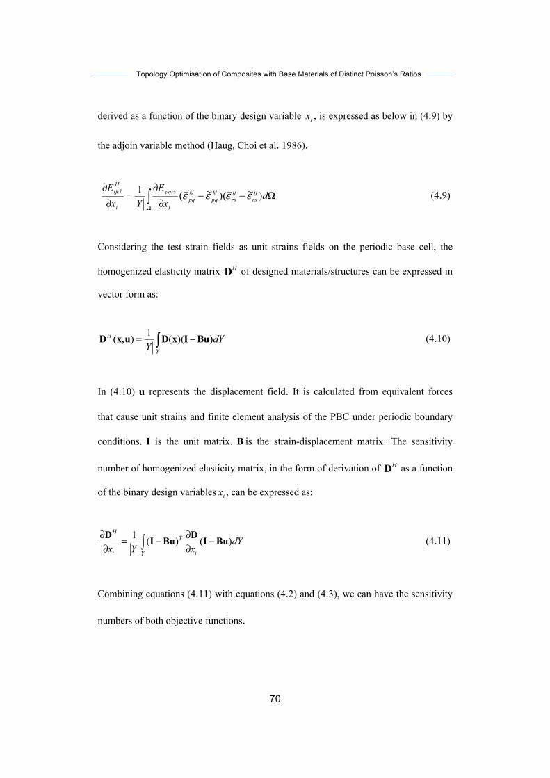
Topology Optimisation of Composites with Base Materials of Distinct Poisson’s Ratios
70
derived as a function of the binary design variable ix , is expressed as below in (4.9) by
the adjoin variable method (Haug, Choi et al. 1986).
∫Ω
Ω−−∂
∂=
∂∂
dxE
YxE ij
rsijrs
klpq
klpq
i
pqrs
i
Hijkl )~)(~(1 εεεε (4.9)
Considering the test strain fields as unit strains fields on the periodic base cell, the
homogenized elasticity matrix HD of designed materials/structures can be expressed in
vector form as:
∫ −=Y
H dYY
))((1)( BuIxDux,D (4.10)
In (4.10) u represents the displacement field. It is calculated from equivalent forces
that cause unit strains and finite element analysis of the PBC under periodic boundary
conditions. I is the unit matrix. B is the strain-displacement matrix. The sensitivity
number of homogenized elasticity matrix, in the form of derivation of HD as a function
of the binary design variables ix , can be expressed as:
∫ −∂∂−=
∂∂
Y i
T
i
H
dYxYx
)()(1 BuIDBuID (4.11)
Combining equations (4.11) with equations (4.2) and (4.3), we can have the sensitivity
numbers of both objective functions.

Topology Optimisation of Composites with Base Materials of Distinct Poisson’s Ratios
71
Up to date on the BESO method, it is usually assumed that the isotropic base material
changes only in the Young’s modulus, not the Poisson’s ratio. Literatures on the
sensitivity with respect to Poisson’s ratio are limited. In this study, base materials can
have not only different Young’s moduli but also their own Poisson’s ratio. To apply the
above analysis to the specific design case of this chapter, below is the derivation for the
sensitivity number of the homogenized elasticity tenser with base materials possessing
different Poisson’s ratios.
For a PBC consisting of different base materials, the elastic tensor is
∑ ∫∑==
⎟⎠⎞⎜
⎝⎛ −−==
NE
e eejj
Ti
TiY
NE
e
eij
Hij dY
YQE
e1
00
1)()(1 εεEεε (4.12)
(i, j=1 to 6 for 3D),
and ejjTi
TiY
eij dYY
Qe
)()(1 00 εεEεε −−= ∫
Where E is the elastic matrix of the base material, 0iε is the i th unit test strain field and
iε is the corresponding induced strain field. eijQ represents the element mutual energy.
The sensitivity of HijE is
dYxYx
Ejj
e
Ti
TiY
e
Hij
e)()(1 00 εεEεε −
∂∂−=
∂∂
∫ (4.13)
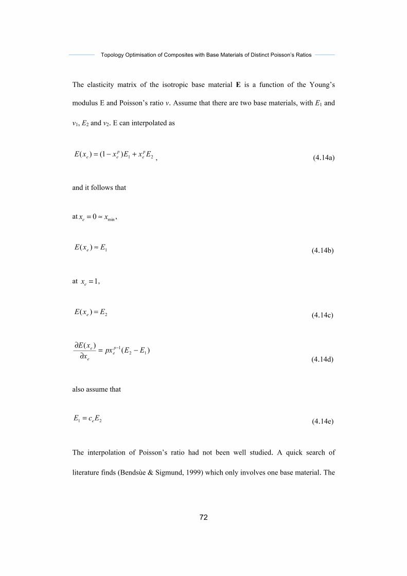
Topology Optimisation of Composites with Base Materials of Distinct Poisson’s Ratios
72
The elasticity matrix of the isotropic base material E is a function of the Young’s
modulus E and Poisson’s ratio v. Assume that there are two base materials, with E1 and
v1, E2 and v2. E can interpolated as
21)1()( ExExxE pe
pee +−= , (4.14a)
and it follows that
at min0 xxe ≈= ,
1)( ExE e ≈ (4.14b)
at 1=ex ,
2)( ExE e = (4.14c)
)()(12
1 EEpxxxE p
ee
e −=∂
∂ −
(4.14d)
also assume that
21 EcE e= (4.14e)
The interpolation of Poisson’s ratio had not been well studied. A quick search of
literature finds (Bendsùe & Sigmund, 1999) which only involves one base material. The
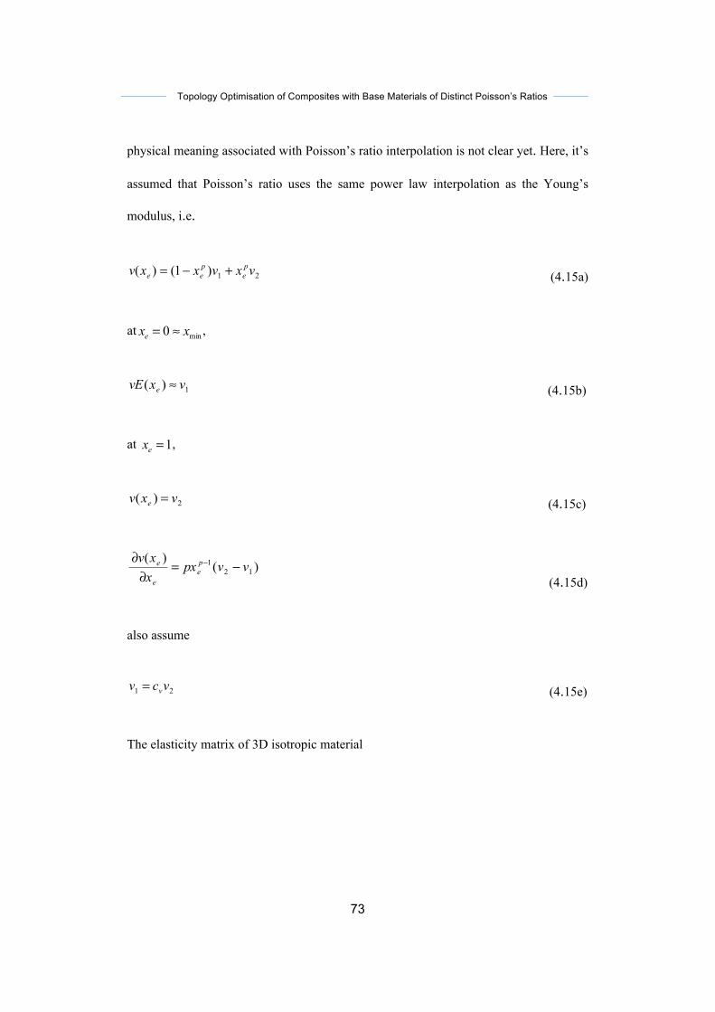
Topology Optimisation of Composites with Base Materials of Distinct Poisson’s Ratios
73
physical meaning associated with Poisson’s ratio interpolation is not clear yet. Here, it’s
assumed that Poisson’s ratio uses the same power law interpolation as the Young’s
modulus, i.e.
21)1()( vxvxxv pe
pee +−= (4.15a)
at min0 xxe ≈= ,
1)( vxvE e ≈ (4.15b)
at 1=ex ,
2)( vxv e = (4.15c)
)()(
121 vvpx
xxv p
ee
e −=∂
∂ −
(4.15d)
also assume
21 vcv v= (4.15e)
The elasticity matrix of 3D isotropic material

Topology Optimisation of Composites with Base Materials of Distinct Poisson’s Ratios
74
)())(21))((1(
)()(2100000
0)(21000000)(21000000)(1)()(000)()(1)(000)()()(1
))(21))((1()()(
eee
e
e
e
e
eee
eee
eee
ee
ee
xxvxv
xE
xvxv
xvxvxvxvxvxvxvxvxvxv
xvxvxE
x
B
EE
−+=
⎥⎥⎥⎥⎥⎥⎥
⎦
⎤
⎢⎢⎢⎢⎢⎢⎢
⎣
⎡
−−
−−
−−
−+==
(4.16)
Also define
⎥⎥⎥⎥⎥⎥⎥⎥
⎦
⎤
⎢⎢⎢⎢⎢⎢⎢⎢
⎣
⎡
−−
−−
−−
=∂
∂=
200000020000002000000111000111000111
)(
e
e
xxBC
, (4.17a)
ejjTi
TiY
eij dYY
Re
)()(1 00 εεCεε −−= ∫ (4.17b)
The 1st order derivative of the elasticity matrix is
cba
e
e
ee
e
ee xxv
xvxxE
xEx
MMM
EEE
++=
∂∂
∂∂+
∂∂
∂∂=
∂∂ )(
)()(
)(
(4.18)
Calculate Ma :
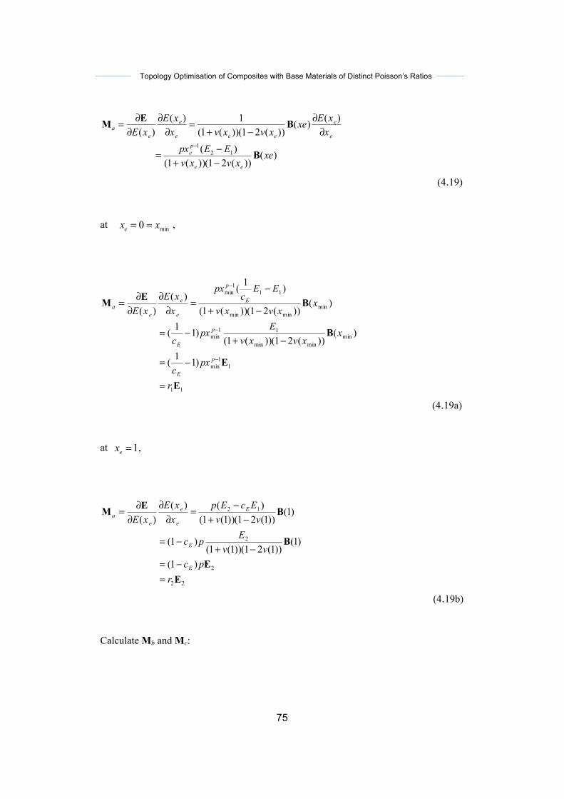
Topology Optimisation of Composites with Base Materials of Distinct Poisson’s Ratios
75
)())(21))((1(
)(
)()())(21))((1(
1)()(
121
xexvxv
EEpx
xxExe
xvxvxxE
xE
ee
pe
e
e
eee
e
ea
B
BEM
−+−=
∂∂
−+=
∂∂
∂∂=
−
(4.19)
at min0 xxe ≈= ,
11
11
min
minminmin
11min
minminmin
111
min
)11(
)())(21))((1(
)11(
)())(21))((1(
)1()(
)(
E
E
B
BEM
r
pxc
xxvxv
Epx
c
xxvxv
EEc
px
xxE
xE
p
E
p
E
E
p
e
e
ea
=
−=
−+−=
−+
−=
∂∂
∂∂=
−
−
−
(4.19a)
at 1=ex ,
22
2
2
12
)1(
)1())1(21))(1(1(
)1(
)1())1(21))(1(1()()(
)(
EE
B
BEM
rpc
vvE
pc
vvEcEp
xxE
xE
E
E
E
e
e
ea
=−=
−+−=
−+−=
∂∂
∂∂=
(4.19b)
Calculate Mb and Mc:
Topology Optimisation of Composites with Base Materials of Distinct Poisson’s Ratios
76
e
e
e
e
ee
e
e
ee
ee
e
ee
e
cbe
e
e
xxv
xx
xvxvxE
xxv
xxvxv
xExvxv
xvxxv
xv
∂∂
∂∂
−++
∂∂
−+−++
+=∂
∂∂∂
)()())(21))((1((
)()()(
))(21))((1(()(
))(21))((1(())(41(
)()(
BB
MME
(4.20)
e
ee
ee
e
ee
eb x
xvx
xvxvxE
xvxvxv
∂∂
−+−++
=)(
)())(21))((1((
)())(21))((1((
))(41(BM
(4.20a)
e
e
e
e
ee
ec x
xvxx
xvxvxE
∂∂
∂∂
−+= )()(
))(21))((1(()( BM
(4.20b)
at min0 xxe ≈= ,
11
111
min11
1
11
min111
1
11
1
)11()21)(1((
)41(
)11())21)(1(()21)(1((
)41(
E
E
BM
s
vc
pxvv
v
vc
pxvv
Evv
v
v
v
p
pb
=
−−+
+−=
−−+−+
+=
−
−
(4.21a)
CCM 111
11
1min )21)(1((
)11( tvv
Evc
pxv
pc =
−+−= −
(4.21b)
at 1=ex ,
Topology Optimisation of Composites with Base Materials of Distinct Poisson’s Ratios
77
22
2222
2
2222
1
22
2
)1()21)(1((
)41(
)1())21)(1(()21)(1((
)41(
E
E
BM
s
vcpvv
v
vcpvv
Evv
v
v
vb
=
−−+
+−=
−−+−+
+=
(4.22a)
CCM 222
22 )21)(1((
)1( tvv
Evcp vc =−+
−=
(4.22b)
Substitute Ma, Mb and Mc to (4.18) then to (4.13) we can have
dYYx
Ejjcba
Ti
TiY
e
Hij
e))()((1 00 εεMMMεε −++−=
∂∂
∫ (4.23)
at min0 xxe ≈= ,
eij
eij
eij
jjTi
TiY
e
Hij
RtQsQr
dYtsrYx
Ee
111
011111
0 ))()((1
++=
−++−=∂∂
∫ εεCEEεε
(4.23a)
at 1=ex ,
eij
eij
eij
jjTi
TiY
e
Hij
RtQsQr
dYtsrYx
Ee
222
011111
0 ))()((1
++=
−++−=∂∂
∫ εεCEEεε
(4.23b)

Topology Optimisation of Composites with Base Materials of Distinct Poisson’s Ratios
78
It’s worth notice that when considering two base materials 21 EE ≠ but common Poisso
n’s ratio 21 vv ≠ , the sensitivity based on (4.23) can be simplified as Mb and Mc being ze
ro matrix.
For cases of 21 EE ≠ and 21 vv ≠ , second order derivative is not taken into consideration
in (4.18) i.e.
e
e
e
e
ee
e
e
ee
e
ee
xxv
xxE
xvxE
xxv
xvxxE
xEx
∂∂
∂∂
∂∂∂
+∂
∂∂∂+
∂∂
∂∂=
∂∂
)()()()(2
1
)()(
)()(2E
EEE
, (4.24)
as the analytical expression for the last term can be very complicated and its impact on
sensitivity number is negligible.
4.1.4. Numerical instabilities and filtering scheme
There are two types of commonly seen numerical instabilities in topology optimization:
mesh dependency and checkerboard patterns. Mesh dependency is a type of instabilities
that result in structures of different effective properties by imposing different mesh sizes
in modeling of the structure. While the checkerboard problem is another type of
instabilities that is mainly caused by numerical errors and emerges when structural
modeling uses low-order finite elements. It appears in the pattern of elements in some
regions of the PBC switching between solid and void by iteration, and may block the
optimization process from convergence. Study by Sigmund and Petersson (Sigmund
Topology Optimisation of Composites with Base Materials of Distinct Poisson’s Ratios
79
and Petersson 1998) shows that by imposing restriction on related design variables both
problems can be avoided to a large extent.
In BESO method both mesh dependency and checkerboard patterns can be solved at the
same time by applying a filtering scheme that is inspired by a related technique used in
image processing (Huang and Xie 2007; Huang and Xie 2010a). The idea of the
filtering scheme is to use the average sensitivity number of one element itself and its
neighboring elements instead of the sensitivity number of only that element (Huang and
Xie 2007; Huang and Xie 2010a). This filtering scheme cuts solid regions with
dimensions smaller than a certain length-scale to appear in the generated topologies by
working as a low-pass filter. After applying the filtering scheme sensitivity number of
each element can be updated by the following equation:
∑
∑
=
== M
jij
N
jjij
i
w
w
1
1ˆα
α (4.25)
Here iα̂ is the updated sensitivity number. ijw is the weight factor. It can be expressed
as:
⎩⎨⎧
≥<−
=min
minmin
for0for
rrrrrr
wij
ijijij (4.26)
Here minr is the filter radius, which will be given as a specific number in design. ijr
represents the distance between the center of element i and j.

Topology Optimisation of Composites with Base Materials of Distinct Poisson’s Ratios
80
In order to help the optimization process reaching a convergent solution under
reasonably fine mesh density, iα̂ needs to be further modified by averaging itself with
its value from previous iteration (Huang and Xie 2007). This further modified
sensitivity number of each elements can be expressed as:
⎪⎩
⎪⎨⎧
+
== − otherwise )ˆˆ(
21
if ˆ~
1ti
ti
ki
i
1k
αα
αα (4.27)
Here superscript t represents current iteration number.
The new updated average sensitivity number iα~ replaces iα̂ from equation (4.25) as the
final sensitivity number of each element. It is used in ranking of all sensitivity numbers
and being recorded to be used in the sensitivity analysis of next iteration. The purpose
of averaging the sensitivity numbers with its iteration histories is to restrain the irregular
swinging of designed regions. The capability of the above filtering procedure for
stabilizing the optimization process is supported by large numbers of numerical
examples (Huang and Xie 2010a).
4.1.5. BESO Procedure
Drawing a summary to the previous sections of this chapter, a whole procedure for
BESO method for maximum bulk or shear modulus can be briefly expressed in the
following steps.
Topology Optimisation of Composites with Base Materials of Distinct Poisson’s Ratios
81
Step 1: Define the BESO parameters, such as prescribed volume fraction *V , filter
radius minr , penalty exponent p (normally )3=p ; evolutionary ratio ER and
mesh density.
Step 2: Create a finite element model for the PBC.
Step 3: Discretise the PBC using FE meshing with periodic boundary condition and unit
strain field. (In 3D problems 6 cases of loading and boundary conditions are
necessary.)
Step 4: Perform finite element analysis (FEA) on the current design and extract the
induced strain fields.
Step 5: Calculate the sensitivity number of each element for the design objective
function by combining equation (4.11) with equation (4.2) and (4.3).
Step 6: Perform the filtering scheme in the PBC design domain using equations (4.25)
and (4.26), and average sensitivity numbers with their historical information
using equation (4.27). Rank the sensitivity numbers of all elements.
Step 7: Define the target volume fraction of stronger elements for the next iteration. If
the current volume fraction of stronger elements tV is larger than the prescribed
volume *V , the target volume for next iteration is calculated
Topology Optimisation of Composites with Base Materials of Distinct Poisson’s Ratios
82
as )),1(max( *VERVV t1t −=+ . Also on the other hand define the target volume
fraction of weaker elements for the next iteration.
Step 8: Determine threshold sensitivity thα for element removal/re-admission. The
threshold sensitivity represents the breaking point on the ranking of sensitivity
numbers of all elements. Elements with a sensitivity number higher than thα
should have a total volume as the target volume fraction of stronger elements
determined in previous step.
Step 9: Redefine the material properties to all elements. For the elements whose
sensitivities are above the threshold ( thi αα ≥ ), they are defined as stronger
elements ( 1=ix ); and vice versa.
Step 10: Check if the remaining total volume of stronger elements meets the prescribed
volume fraction and if the optimization process satisfies the convergence
criterion.
Step 11: Repeat steps 2 to 10 until both the prescribed volume fraction and the
convergence criterion are satisfied.
The above-mentioned convergence criterion is defined by changes of the effective value
of the objective function (K or G ) over iterations, as seen in equation (4.28).

Topology Optimisation of Composites with Base Materials of Distinct Poisson’s Ratios
83
τη
θ
≤−
∑
∑
=
+−
=
+−−+−
1
1
1
11 )(
i
it
i
iNtit
f
ff (4.28)
Here f represents the effective value of the objective function. θ stands for the
summation upper bound. τ represents the prescribed convergence tolerance. θ is
usually set to 5 and τ is usually set to 0.1%. By applying these numbers to (4.28), it
can be explained as convergence is reached under the condition that the changes of the
effective value of the objective function over the last 10 iterations is equal to or less
than 0.1%.
4.2. Results and Discussion
4.2.1 Composites with maximum bulk modulus
Selected case study shown in this section use a cubic design domain, which is
discretized into 30×30×30 8-node brick elements. Each element is with dimensions 1
unit × 1 unit × 1 unit. Three sets of samples are studied, representing three assortments
of Poison’s rations of base materials. The optimization objective is to achieve maximum
bulk modulus, subject to volume fraction of 50% for each base material. Here as shown
in Figure 4.1, the initial material distribution consists eight soft-material elements at the
center of PBC while hard material assigned to all other elements.
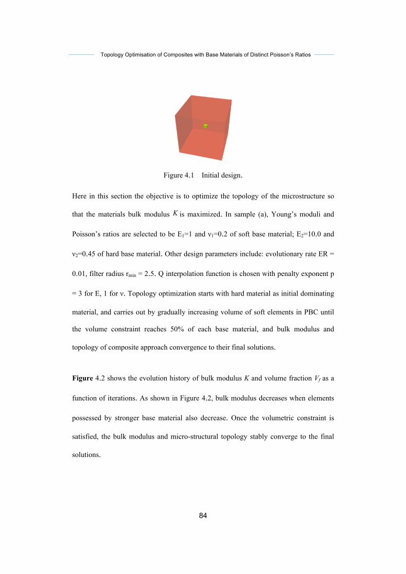
Topology Optimisation of Composites with Base Materials of Distinct Poisson’s Ratios
84
Here in this section the objective is to optimize the topology of the microstructure so
that the materials bulk modulus K is maximized. In sample (a), Young’s moduli and
Poisson’s ratios are selected to be E1=1 and ν1=0.2 of soft base material; E2=10.0 and
ν2=0.45 of hard base material. Other design parameters include: evolutionary rate ER =
0.01, filter radius rmin = 2.5. Q interpolation function is chosen with penalty exponent p
= 3 for E, 1 for ν. Topology optimization starts with hard material as initial dominating
material, and carries out by gradually increasing volume of soft elements in PBC until
the volume constraint reaches 50% of each base material, and bulk modulus and
topology of composite approach convergence to their final solutions.
Figure 4.2 shows the evolution history of bulk modulus K and volume fraction Vf as a
function of iterations. As shown in Figure 4.2, bulk modulus decreases when elements
possessed by stronger base material also decrease. Once the volumetric constraint is
satisfied, the bulk modulus and micro-structural topology stably converge to the final
solutions.
Figure 4.1 Initial design.
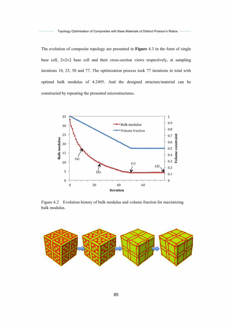
Topology Optimisation of Composites with Base Materials of Distinct Poisson’s Ratios
85
The evolution of composite topology are presented in Figure 4.3 in the form of single
base cell, 2×2×2 base cell and their cross-section views respectively, at sampling
iterations 10, 25, 50 and 77. The optimization process took 77 iterations in total with
optimal bulk modulus of 4.2495. And the designed structure/material can be
constructed by repeating the presented microstructures.
Figure 4.2 Evolution history of bulk modulus and volume fraction for maximizing bulk modulus.
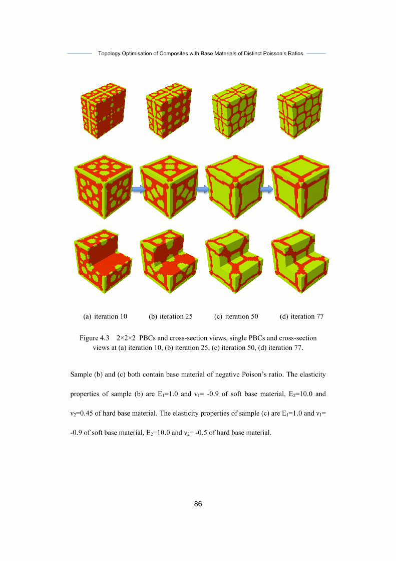
Topology Optimisation of Composites with Base Materials of Distinct Poisson’s Ratios
86
(a) iteration 10 (b) iteration 25 (c) iteration 50 (d) iteration 77
Figure 4.3 2×2×2 PBCs and cross-section views, single PBCs and cross-section views at (a) iteration 10, (b) iteration 25, (c) iteration 50, (d) iteration 77.
Sample (b) and (c) both contain base material of negative Poison’s ratio. The elasticity
properties of sample (b) are E1=1.0 and ν1= -0.9 of soft base material, E2=10.0 and
ν2=0.45 of hard base material. The elasticity properties of sample (c) are E1=1.0 and ν1=
-0.9 of soft base material, E2=10.0 and ν2= -0.5 of hard base material.
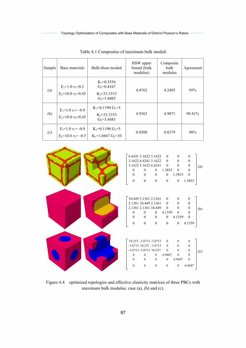
Topology Optimisation of Composites with Base Materials of Distinct Poisson’s Ratios
87
Table 4.1 Composites of maximum bulk moduli
Sample Base materials Bulk/shear moduli HSW upper bound (bulk
modulus)
Composite bulk
modulus Agreement
(a) E1=1.0 ν1=0.2
E2=10.0 ν2=0.45
K1=0.5556 G1=0.4167
K2=33.3333 G2=3.4483
4.4762 4.2495 95%
(b) E1=1.0 ν1= -0.9
E2=10.0 ν2=0.45
K1=0.1190 G1=5
K2=33.3333 G2=3.4483
4.9363 4.9071 99.41%
(c) E1=1.0 ν1= -0.9
E2=10.0 ν2= -0.5
K1=0.1190 G1=5
K2=1.6667 G2=10 0.8508 0.8379 98%
6.4241 3.1622 3.1622 0 0 0
3.1622 6.4241 3.1622 0 0 0 3.1622 3.1622 6.4241 0 0 0
0 0 0 1.3853 0 0 0 0 0 0 1.3853 0
0 0 0 0 0 1.3853
(a)
10.449 2.1361 2.1361 0 0 0
2.1361 10.449 2.1361 0 0 0 2.1361 2.1361 10.449 0 0 0
0 0 0 4.1359 0 0 0 0 0 0 4.1359 0
0 0 0 0 0 4.1359
(b)
10.257 -3.8713 -3.8713 0 0 0
-3.8713 10.257 -3.8713 0 0 0 -3.8713 -3.8713 10.257 0 0 0
0 0 0 6.9687 0 0 0 0 0 0 6.9687 0
0 0 0 0 0 6.9687
(c)
Figure 4.4 optimized topologies and effective elasticity matrices of three PBCs with maximum bulk modulus: case (a), (b) and (c).

Topology Optimisation of Composites with Base Materials of Distinct Poisson’s Ratios
88
Table 4.2 parameters and results for best solution under each condition (cubic symmetric model)
Maximising bulk
modulus
Base materials
Filter radius (rmin)
ER Mesh density
Interpolation function Iterations Bulk
modulus Shear
modulus
E1=1.0 ν1=0.2
E2=10.0 ν2=0.45
2.5 0.01 303 Q 77 4.2495 1.3853
E1=1.0 ν1= -0.9 E2=10.0 ν2=0.45
1.5 0.01 303 Q 66 4.9071 4.1359
E1=1.0 ν1= -0.9 E2=10.0 ν2=-0.5
3.0 0.01 303 SIMP 61 0.8379 6.9687
4.2.2 Composites with maximum shear modulus
Here in this section the objective is to optimize the topology of the microstructure so
that the materials shear modulus is maximized. Case studies use the same initial
design as in previous section as shown in Figure 4.1.
Below in sample (a), Young’s moduli and Poisson’s ratios are selected to be E1=1 and
ν1=0.2 of soft base material; E2=10.0 and ν2=0.45 of hard base material. Other design
parameters include: evolutionary rate ER = 0.01, filter radius rmin = 2.5. SIMP
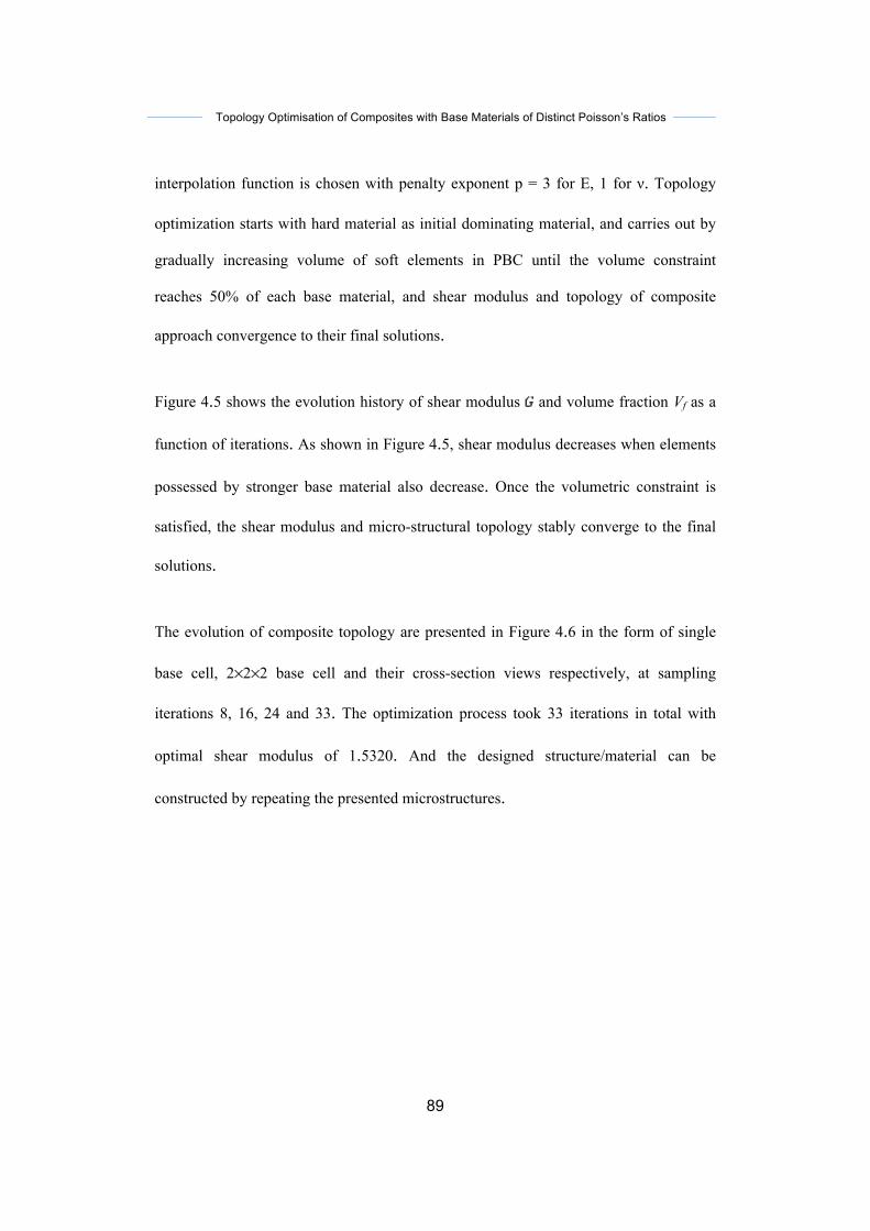
Topology Optimisation of Composites with Base Materials of Distinct Poisson’s Ratios
89
interpolation function is chosen with penalty exponent p = 3 for E, 1 for ν. Topology
optimization starts with hard material as initial dominating material, and carries out by
gradually increasing volume of soft elements in PBC until the volume constraint
reaches 50% of each base material, and shear modulus and topology of composite
approach convergence to their final solutions.
Figure 4.5 shows the evolution history of shear modulus and volume fraction Vf as a
function of iterations. As shown in Figure 4.5, shear modulus decreases when elements
possessed by stronger base material also decrease. Once the volumetric constraint is
satisfied, the shear modulus and micro-structural topology stably converge to the final
solutions.
The evolution of composite topology are presented in Figure 4.6 in the form of single
base cell, 2×2×2 base cell and their cross-section views respectively, at sampling
iterations 8, 16, 24 and 33. The optimization process took 33 iterations in total with
optimal shear modulus of 1.5320. And the designed structure/material can be
constructed by repeating the presented microstructures.
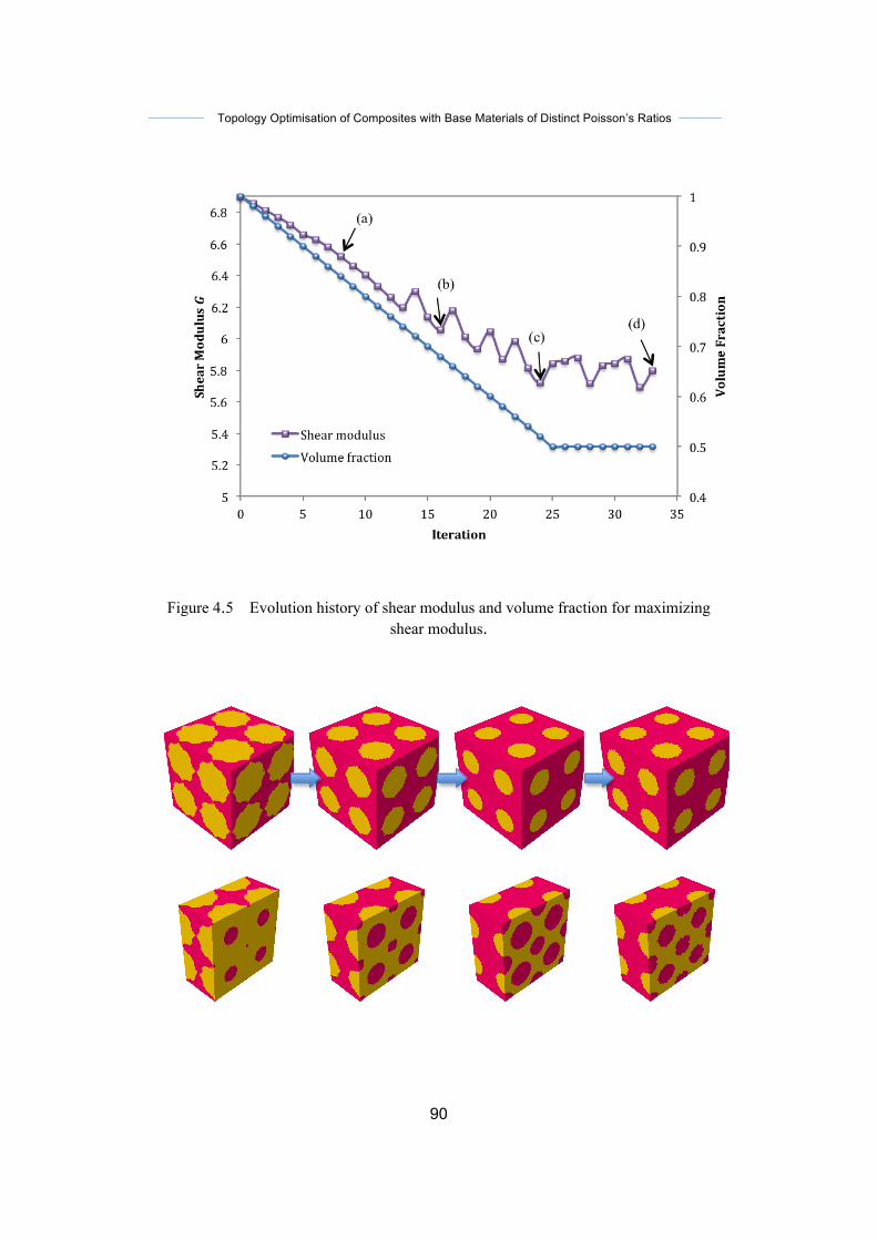
Topology Optimisation of Composites with Base Materials of Distinct Poisson’s Ratios
90
Figure 4.5 Evolution history of shear modulus and volume fraction for maximizing shear modulus.
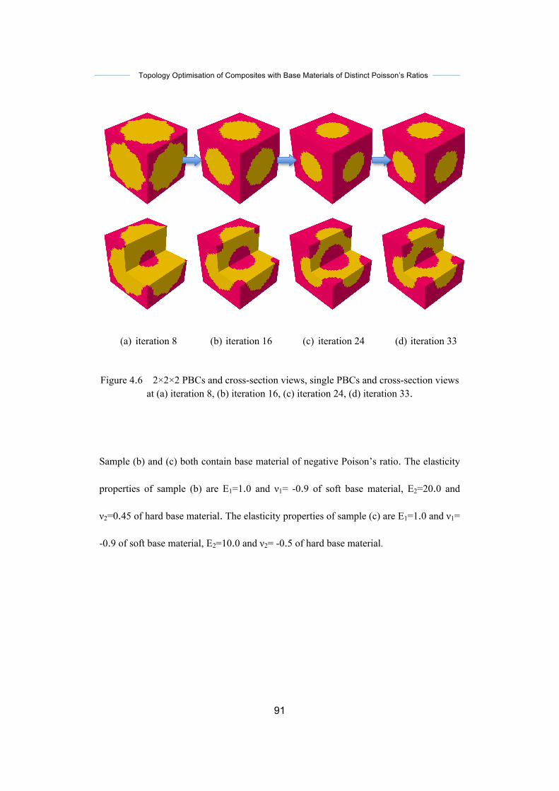
Topology Optimisation of Composites with Base Materials of Distinct Poisson’s Ratios
91
(a) iteration 8 (b) iteration 16 (c) iteration 24 (d) iteration 33
Figure 4.6 2×2×2 PBCs and cross-section views, single PBCs and cross-section views at (a) iteration 8, (b) iteration 16, (c) iteration 24, (d) iteration 33.
Sample (b) and (c) both contain base material of negative Poison’s ratio. The elasticity
properties of sample (b) are E1=1.0 and ν1= -0.9 of soft base material, E2=20.0 and
ν2=0.45 of hard base material. The elasticity properties of sample (c) are E1=1.0 and ν1=
-0.9 of soft base material, E2=10.0 and ν2= -0.5 of hard base material.
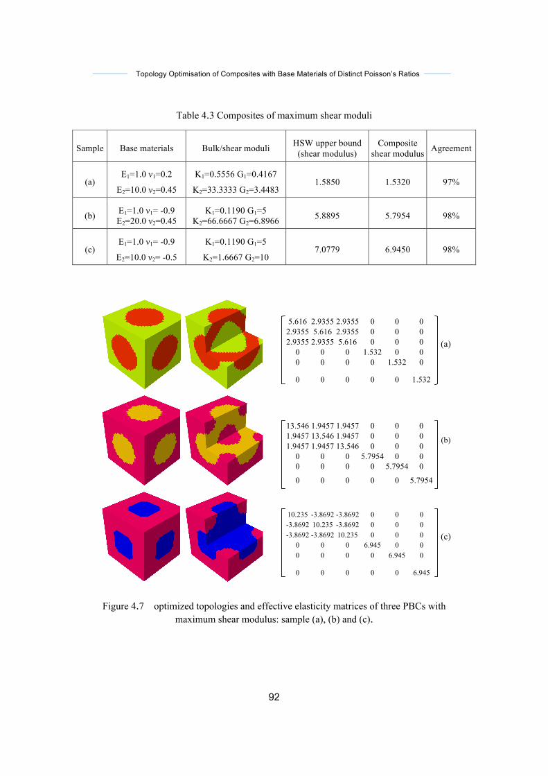
Topology Optimisation of Composites with Base Materials of Distinct Poisson’s Ratios
92
Table 4.3 Composites of maximum shear moduli
Sample Base materials Bulk/shear moduli HSW upper bound (shear modulus)
Composite shear modulus Agreement
(a) E1=1.0 ν1=0.2
E2=10.0 ν2=0.45
K1=0.5556 G1=0.4167
K2=33.3333 G2=3.4483 1.5850 1.5320 97%
(b) E1=1.0 ν1= -0.9 E2=20.0 ν2=0.45
K1=0.1190 G1=5 K2=66.6667 G2=6.8966 5.8895 5.7954 98%
(c) E1=1.0 ν1= -0.9
E2=10.0 ν2= -0.5
K1=0.1190 G1=5
K2=1.6667 G2=10 7.0779 6.9450 98%
5.616 2.9355 2.9355 0 0 0
2.9355 5.616 2.9355 0 0 0 2.9355 2.9355 5.616 0 0 0
0 0 0 1.532 0 0 0 0 0 0 1.532 0
0 0 0 0 0 1.532
(a)
13.546 1.9457 1.9457 0 0 0
1.9457 13.546 1.9457 0 0 0 1.9457 1.9457 13.546 0 0 0
0 0 0 5.7954 0 0 0 0 0 0 5.7954 0
0 0 0 0 0 5.7954
(b)
10.235 -3.8692 -3.8692 0 0 0
-3.8692 10.235 -3.8692 0 0 0 -3.8692 -3.8692 10.235 0 0 0
0 0 0 6.945 0 0 0 0 0 0 6.945 0
0 0 0 0 0 6.945
(c)
Figure 4.7 optimized topologies and effective elasticity matrices of three PBCs with maximum shear modulus: sample (a), (b) and (c).
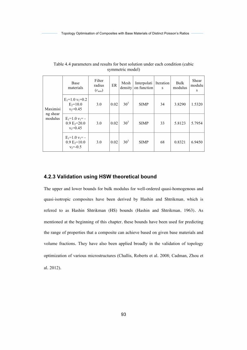
Topology Optimisation of Composites with Base Materials of Distinct Poisson’s Ratios
93
Table 4.4 parameters and results for best solution under each condition (cubic symmetric model)
Maximising shear modulus
Base materials
Filter radius (rmin)
ER Mesh density
Interpolation function
Iterations
Bulk modulus
Shear modulu
s
E1=1.0 ν1=0.2 E2=10.0 ν2=0.45
3.0 0.02 303 SIMP 34 3.8290 1.5320
E1=1.0 ν1= -0.9 E2=20.0 ν2=0.45
3.0 0.02 303 SIMP 33 5.8123 5.7954
E1=1.0 ν1= -0.9 E2=10.0 ν2=-0.5
3.0 0.02 303 SIMP 68 0.8321 6.9450
4.2.3 Validation using HSW theoretical bound
The upper and lower bounds for bulk modulus for well-ordered quasi-homogenous and
quasi-isotropic composites have been derived by Hashin and Shtrikman, which is
refered to as Hashin Shtrikman (HS) bounds (Hashin and Shtrikman, 1963). As
mentioned at the beginning of this chapter, these bounds have been used for predicting
the range of properties that a composite can achieve based on given base materials and
volume fractions. They have also been applied broadly in the validation of topology
optimization of various microstructures (Challis, Roberts et al. 2008; Cadman, Zhou et
al. 2012).
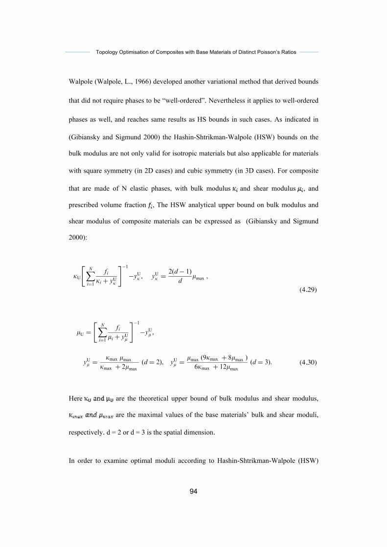
Topology Optimisation of Composites with Base Materials of Distinct Poisson’s Ratios
94
Walpole (Walpole, L., 1966) developed another variational method that derived bounds
that did not require phases to be “well-ordered”. Nevertheless it applies to well-ordered
phases as well, and reaches same results as HS bounds in such cases. As indicated in
(Gibiansky and Sigmund 2000) the Hashin-Shtrikman-Walpole (HSW) bounds on the
bulk modulus are not only valid for isotropic materials but also applicable for materials
with square symmetry (in 2D cases) and cubic symmetry (in 3D cases). For composite
that are made of N elastic phases, with bulk modulus and shear modulus , and
prescribed volume fraction , The HSW analytical upper bound on bulk modulus and
shear modulus of composite materials can be expressed as (Gibiansky and Sigmund
2000):
!"#$%& '"( )*+ )(,$&-+(&+./ 0&")("102 2"31"&0)+& 40)* 2/.0$%(02,. 0$2.#&0"$&5 6*+1*,&+& 4+(+ "&+% )" !+ 74+..8"(%+(+%9 &" )*,) )*+ 1*,&+ 40)* )*+ .,(:+&);&3,..+&)< !#.= 3"%#.#& ,.&" *,% )*+ .,(:+&) ;&3,..+&)< &*+,( 3"%#.#&5 >,.1".+;?@AA< %+-+."1+% , &030.,( -,(0,)0"$,. 3+)*"% ,$% %+(0-+% !"#$%& )*,) %0% $")(+B#0(+ ,$/ 1*,&+ "(%+(0$:5 C"( )*+ 4+..8"(%+(+% 1*,&+&D )*+ >,.1".+ !"#$%& ,(++B#0-,.+$) )" )*+ EF "$+&5
6*+ EF> !"#$%& *,-+ )*+ '"(3
!!!!!!!"D "!!"!!""D "##
4*+(+
!!
!"!
"$?
#"!" % $!!
#&?
&$!! D $!! $ G"%& ?#%
"$%& D "'#
!"
!"!
"$?
#"!" % $"!
#&?
&$"! D $"! $ G"%& ?#%
"$() D "*#
"! $!"!
"$?
#""" % $!"
#&?
&$!" D
$!" $ !$%& "$%&
!$%& % G"$%&
"% $ G#D $!" $ "$%& "@!$%& % H"$%& #A!$%& % ?G"$%&
"% $ I#D "+#
"" $!"!
"$?
#""" % $""
#&?
&$"" D
$"" $ !$() "$()
!$() % G"$()
"% $ G#D $"" $ "$() "@!$() % H"$() #A!$() % ?G"$()
"% $ I#! ",#
E+(+D !30$ ;!3,J< ,$% "30$ ;"3,J< ,(+ )*+ 30$03,. ;3,J03,.< -,.#+& "' )*+ 1*,&+!#.= ,$% &*+,( 3"%#.0D (+&1+2)0-+./D ,$% % K G "( % K I 0& )*+ &1,)0,. %03+$&0"$5
L) 0& =$"4$ )*,) )*+ )4"81*,&+ EF !"#$%& ;?< ;% K G< ,(+ "1)03,. 0$ )*+ &+$&+)*,) )*+(+ +J0&) &1+20,. 302("&)(#2)#(+& ;E,&*0$ ,$% F*)(0=3,$D ?@AI< 40)* ,$+M+2)0-+ !#.= 3"%#.0 +B#,. )" !N ,$% !O5 L) 0& ,.&" =$"4$ )*,) '"( 3"(+ )*,$ )4"1*,&+& )*+&+ !"#$%& 2,$$") !+ "1)03,. 0$ )*+ 4*".+ (,$:+ "' 1,(,3+)+(&5 L$%++%D2"$&0%+( )*+ #11+( !"#$% !O '"( )*+ &0)#,)0"$ 4*+(+ )*+ -".#3+ '(,2)0"$ "' )*+&)0M 1*,&+ ;40)* .,(:+ !#) P$0)+ &*+,( 3"%#.#& "&"3,J< -,$0&*+&5 Q$+ 2,$ &++)*,) )*+ !"#$% &)0.. %+1+$%& "$ )*+ &*+,( 3"%#.#& "' )*+ 1*,&+ 40)* R+(" -".#3+'(,2)0"$5 E"4+-+(D +M+2)0-+ 3"%#.0 "' ,$/ 2"31"&0)+ 2,$$") %+1+$% "$ )*+3"%#.0 "' )*+ 1*,&+ 40)* P$0)+ 3"%#.0 ,$% R+(" -".#3+ '(,2)0"$5
'()( *"+",-./$0 1( 2"345-% 6 7( 89:;( <;$.( 2=>"%. ?@ ABCCCD ?EFG?H@SAS
(4.29)
!"#$%& '"( )*+ )(,$&-+(&+./ 0&")("102 2"31"&0)+& 40)* 2/.0$%(02,. 0$2.#&0"$&5 6*+1*,&+& 4+(+ "&+% )" !+ 74+..8"(%+(+%9 &" )*,) )*+ 1*,&+ 40)* )*+ .,(:+&);&3,..+&)< !#.= 3"%#.#& ,.&" *,% )*+ .,(:+&) ;&3,..+&)< &*+,( 3"%#.#&5 >,.1".+;?@AA< %+-+."1+% , &030.,( -,(0,)0"$,. 3+)*"% ,$% %+(0-+% !"#$%& )*,) %0% $")(+B#0(+ ,$/ 1*,&+ "(%+(0$:5 C"( )*+ 4+..8"(%+(+% 1*,&+&D )*+ >,.1".+ !"#$%& ,(++B#0-,.+$) )" )*+ EF "$+&5
6*+ EF> !"#$%& *,-+ )*+ '"(3
!!!!!!!"D "!!"!!""D "##
4*+(+
!!
!"!
"$?
#"!" % $!!
#&?
&$!! D $!! $ G"%& ?#%
"$%& D "'#
!"
!"!
"$?
#"!" % $"!
#&?
&$"! D $"! $ G"%& ?#%
"$() D "*#
"! $!"!
"$?
#""" % $!"
#&?
&$!" D
$!" $ !$%& "$%&
!$%& % G"$%&
"% $ G#D $!" $ "$%& "@!$%& % H"$%& #A!$%& % ?G"$%&
"% $ I#D "+#
"" $!"!
"$?
#""" % $""
#&?
&$"" D
$"" $ !$() "$()
!$() % G"$()
"% $ G#D $"" $ "$() "@!$() % H"$() #A!$() % ?G"$()
"% $ I#! ",#
E+(+D !30$ ;!3,J< ,$% "30$ ;"3,J< ,(+ )*+ 30$03,. ;3,J03,.< -,.#+& "' )*+ 1*,&+!#.= ,$% &*+,( 3"%#.0D (+&1+2)0-+./D ,$% % K G "( % K I 0& )*+ &1,)0,. %03+$&0"$5
L) 0& =$"4$ )*,) )*+ )4"81*,&+ EF !"#$%& ;?< ;% K G< ,(+ "1)03,. 0$ )*+ &+$&+)*,) )*+(+ +J0&) &1+20,. 302("&)(#2)#(+& ;E,&*0$ ,$% F*)(0=3,$D ?@AI< 40)* ,$+M+2)0-+ !#.= 3"%#.0 +B#,. )" !N ,$% !O5 L) 0& ,.&" =$"4$ )*,) '"( 3"(+ )*,$ )4"1*,&+& )*+&+ !"#$%& 2,$$") !+ "1)03,. 0$ )*+ 4*".+ (,$:+ "' 1,(,3+)+(&5 L$%++%D2"$&0%+( )*+ #11+( !"#$% !O '"( )*+ &0)#,)0"$ 4*+(+ )*+ -".#3+ '(,2)0"$ "' )*+&)0M 1*,&+ ;40)* .,(:+ !#) P$0)+ &*+,( 3"%#.#& "&"3,J< -,$0&*+&5 Q$+ 2,$ &++)*,) )*+ !"#$% &)0.. %+1+$%& "$ )*+ &*+,( 3"%#.#& "' )*+ 1*,&+ 40)* R+(" -".#3+'(,2)0"$5 E"4+-+(D +M+2)0-+ 3"%#.0 "' ,$/ 2"31"&0)+ 2,$$") %+1+$% "$ )*+3"%#.0 "' )*+ 1*,&+ 40)* P$0)+ 3"%#.0 ,$% R+(" -".#3+ '(,2)0"$5
'()( *"+",-./$0 1( 2"345-% 6 7( 89:;( <;$.( 2=>"%. ?@ ABCCCD ?EFG?H@SAS
(4.30)
Here are the theoretical upper bound of bulk modulus and shear modulus,
are the maximal values of the base materials’ bulk and shear moduli,
respectively. d = 2 or d = 3 is the spatial dimension.
In order to examine optimal moduli according to Hashin-Shtrikman-Walpole (HSW)

Topology Optimisation of Composites with Base Materials of Distinct Poisson’s Ratios
95
bounds, here we choose two sets of base materials to form two-phase composites. The
Hashin-Shtrikman-Walpole (HSW) upper bounds on effective bulk and shear moduli of
potential composites can be calculated as shown in Table 4.5.
Table 4.5 Two composites and their corresponding HSW upper bounds
(Target volume=50%)
Sample Base materials Bulk/shear moduli HSW upper bound (bulk modulus)
HSW upper bound
(shear modulus)
(a) E1=1.0 ν1= 0.3
(E2=10-9 ν2=0.3)
K1= 0.8333 G1= 0.3846
K2=0 G2=0 0.2299 0.1322
(b) E1=1.0 ν1=0.2
E2=10.0 ν2=0.2
K1=0.5556 G1=0.4167
K2=5.5556 G2=4.1667 2.3297 1.7473
The HSW upper bounds of bulk modulus Ku are attainable subject to the restrictions:
If K1 ≤ K2 , the HSW upper bound is attainable if
G1 ≥G2, Ku ≤ K2 , (4.31a)
Or if
G2 ≥G1, Ku ≥ K1 , (4.31b)
and vice versa. Both composites here satisfy (4.31). Therefore their bulk moduli K have
the potential to achieve upper bounds Ku .
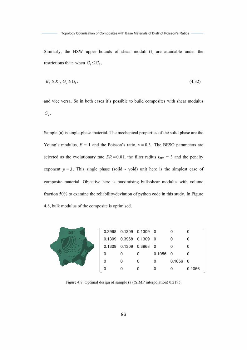
Topology Optimisation of Composites with Base Materials of Distinct Poisson’s Ratios
96
Similarly, the HSW upper bounds of shear moduli Gu are attainable under the
restrictions that: when G1 ≤G2 ,
K2 ≥ K1, Gu ≥G1 . (4.32)
and vice versa. So in both cases it’s possible to build composites with shear modulus
Gu .
Sample (a) is single-phase material. The mechanical properties of the solid phase are the
Young’s modulus, E = 1 and the Poisson’s ratio, 3.0=v . The BESO parameters are
selected as the evolutionary rate =ER 0.01, the filter radius rmin = 3 and the penalty
exponent 3=p . This single phase (solid - void) unit here is the simplest case of
composite material. Objective here is maximising bulk/shear modulus with volume
fraction 50% to examine the reliability/deviation of python code in this study. In Figure
4.8, bulk modulus of the composite is optimised.
0.3968 0.1309 0.1309 0 0 0
0.1309 0.3968 0.1309 0 0 0
0.1309 0.1309 0.3968 0 0 0
0 0 0 0.1056 0 0
0 0 0 0 0.1056 0
0 0 0 0 0 0.1056
Figure 4.8. Optimal design of sample (a) (SIMP interpolation) 0.2195.

Topology Optimisation of Composites with Base Materials of Distinct Poisson’s Ratios
97
The following case is two-phase composite material. Its mechanical properties are the
Young’s moduli, E1=1.0 E2=10.0 and the Poisson’s ratio, ν1=0.2 ν2=0.2 too. The BESO
parameters are chosen as the evolutionary rate =ER 0.01, the filter radius rmin = 3 and
the penalty exponent 3=p . In Figure 4.9, bulk modulus of the composite is optimised.
4.3515 0.8481 0.8481 0 0 0
0.8481 4.3515 0.8481 0 0 0
0.8481 0.8481 4.3515 0 0 0
0 0 0 1.3162 0 0
0 0 0 0 1.3162 0
0 0 0 0 0 1.3162
Figure 4.9. Optimal design of sample (b) (SIMP interpolation) 2.0159.
Below in Figure 4.10 and Figure 4.11, shear moduli of both samples are optimised.
0.3545 0.1511 0.1511 0 0 0
0.1511 0.3545 0.1511 0 0 0
0.1511 0.1511 0.3545 0 0 0
0 0 0 0.1305 0 0
0 0 0 0 0.1305 0
0 0 0 0 0 0.1305
Figure 4.10. Optimal design of sample (a) (SIMP interpolation) 0.1305.
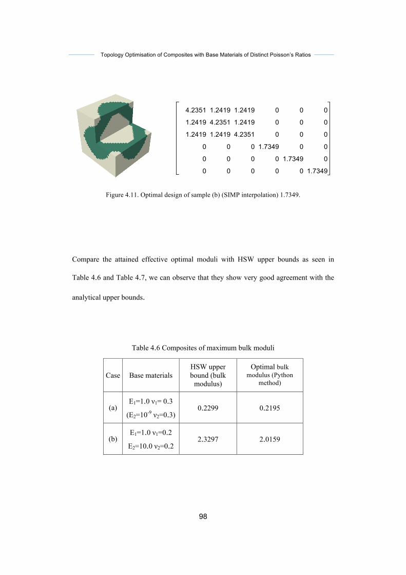
Topology Optimisation of Composites with Base Materials of Distinct Poisson’s Ratios
98
4.2351 1.2419 1.2419 0 0 0
1.2419 4.2351 1.2419 0 0 0
1.2419 1.2419 4.2351 0 0 0
0 0 0 1.7349 0 0
0 0 0 0 1.7349 0
0 0 0 0 0 1.7349
Figure 4.11. Optimal design of sample (b) (SIMP interpolation) 1.7349.
Compare the attained effective optimal moduli with HSW upper bounds as seen in
Table 4.6 and Table 4.7, we can observe that they show very good agreement with the
analytical upper bounds.
Table 4.6 Composites of maximum bulk moduli
Case Base materials HSW upper bound (bulk
modulus)
Optimal bulk modulus (Python
method)
(a) E1=1.0 ν1= 0.3
(E2=10-9 ν2=0.3) 0.2299 0.2195
(b) E1=1.0 ν1=0.2
E2=10.0 ν2=0.2 2.3297 2.0159
Topology Optimisation of Composites with Base Materials of Distinct Poisson’s Ratios
99
Table 4.7 Composites of maximum shear moduli
Case Base materials HSW upper bound (shear
modulus)
Optimal shear modulus (Python
method)
(a) E1=1.0 ν1= 0.3
(E2=10-9 ν2=0.3) 0.1322 0.1305
(b) E1=1.0 ν1=0.2
E2=10.0 ν2=0.2 1.7473 1.7349
4.3. Concluding remarks
In this chapter the BESO method has been developed into the designing of two-phase
composites with maximum bulk modulus or shear modulus. The idea of BESO method
is to seek optimal material spatial distribution within periodic base cell by performing
topology optimization subject to volume constraints. With the help of homogenization
theory, the overall effective properties of design domain can be calculated. Sensitivity
analysis is carried out in each iteration also utilising the homogenization theory. The
binary design variable , which marks the density of elements, is redefined elementally
based on ranking of sensitivity numbers of all elements in PBC. The optimization
process gradually evolves towards on optimal solution as well as satisfying both
prescribed volume constraint and convergence criterion.
In this study ABAQUS was used as the FE analysis tool, and the BESO part is
implemented as a “post-processor” in Python code. Several case studies are presented to
demonstrate the effectiveness of the proposed BESO method. The known HSW

Topology Optimisation of Composites with Base Materials of Distinct Poisson’s Ratios
100
analytical bounds are used for verifications of the results. Some interesting topological
patterns have been found for guiding the composite material design. The method is the
first one that predicts optimal bulk/shear modulus of composites possessing base
materials of different Poisson’s ratio. The methodology developed in this chapter can be
further extended to various other material design scenarios easily.
Topology Optimisation of Composites with Base Materials of Distinct Poisson’s Ratios
101
Chapter5ConclusionsandRecommendations
5.1. Conclusions
This thesis has presented a new approach for the design of microstructures of materials
with different Poisson’s ratio using the BESO method. It is assumed that the materials
are composed of periodic base cells. A new algorithm for composite material design
Topology Optimisation of Composites with Base Materials of Distinct Poisson’s Ratios
102
with extreme Young's moduli has been developed and then the new procedure for
design of two-phase composite materials with base materials possessing different
Poisson's ratio has also been proposed. The main conclusions can be obtained from this
thesis as follows,
�� a computational algorithm for topological design of composite materials with
extreme Young’s moduli has been developed. The composite consists of base materials
with different Poisson’s ratios. The elemental sensitivity analysis has been carried out
using finite element modelling and the homogenization theory. Based on the sensitivity
ranking, the optimal topology for the PBC is obtained. Numerical results show that the
proposed algorithm is effective and computational efficient. The modulus of the
composite is much higher than that of base materials. When one of the base materials
has negative Poisson's ratio, the modulus of the composite increases significantly.
�� a computational algorithm for topological design of two-phase composite
materials with extreme bulk or shear modulus has been developed. These composites
possess two different materials phases. The algorithm is to achieve the optimal material
spatial distribution within periodic base cell by performing topology optimization
subject to the volume constraints. The homogenization theory is adopted to build the
relationship between the material properties of the whole design body in macrostructure
scope and that of the periodic base cell in microstructure scope. The sensitivity analysis
is carried out in each iteration to achieve an optimal solution. Several case studies have
been presented to demonstrate the effectiveness of the proposed algorithm.

Topology Optimisation of Composites with Base Materials of Distinct Poisson’s Ratios
103
5.2. Recommendations
The approach for the design of microstructures of materials with different Poisson’s
ratio using the BESO method has been presented in this thesis. Several case studies
have been carried out to show the effectiveness and computation efficiency of the
proposed approach. Some further work is listed as follows:
�� More case studies should be carried out next step to broaden applications of the
developed algorithm.
�� Other objective functions such as frequency and thermal expansion could be
considered.
�� It would be worthwhile extending the present study to the concurrent
optimisation of both macrostructure and material microstructure of composites with
multiple phases of distinct Poisson’s ratios.
Topology Optimisation of Composites with Base Materials of Distinct Poisson’s Ratios
104
Reference
Allaire, G., F. Jouve, et al. (2004). "Structural optimization using sensitivity analysis
and a level-set method." Journal of Computational Physics 194(1): 363-393.
Asaadi, J. (1973). "A computational comparison of some non-linear programs."
Mathematical Programming 4(1): 144-154.
Bendsøe, M. P. (1989). "Optimal shape design as a material distribution problem."
Structural and Multidisciplinary Optimization 1(4): 193-202.
Bendsøe, M. P. (1989). "Optimal shape design as a material distribution problem."
Structural and Multidisciplinary Optimization 1(4): 193-202.
Bendsøe, M. P. and N. Kikuchi (1988). "Generating optimal topologies in structural
design using a homogenization method." Computer Methods in Applied
Mechanics and Engineering 71(2): 197-224.
Bendsøe, M. P. and N. Kikuchi (1988). "Generating optimal topologies in optimal
design using a homogenization method." Comp. Meth. Appl. Mech. Eng. 71:
197-224.
Bendsøe, M. P. and N. Kikuchi (1988). "Generating optimal topologies in structural
design using a homogenization method." Computer Methods in Applied
Mechanics and Engineering 71(2): 197-224.
Bendsøe, M. P. and N. Kikuchi (1988). "Generating optimal topologies in structural
design using a homogenization method." Computer Methods in Applied
Mechanics and Engineering 71(2): 197-224.
Bendsøe, M. P. and N. Kikuchi (1988). "Generating optimal topologies in optimal
design using a homogenization method." Comp. Meth. Appl. Mech. Eng. 71:
197-224.
Bendsøe, M. P. and O. Sigmund (1999). "Material interpolation schemes in topology
optimization." Archive of Applied Mechanics 69(9): 635-654.
Topology Optimisation of Composites with Base Materials of Distinct Poisson’s Ratios
105
Bendsøe, M. P. and O. Sigmund (2003). Topology Optimization: Theory, Methods
and Application. Berlin, Springer.
Bendsøe, M. P., J. M. Guedes, et al. (1993). "An Analytical Model to Predict Optimal
Material Properties in the Context of Optimal Structural Design." Journal of
Applied Mechanics 61(4): 930-937.
Bendsøe, M.P. and Sigmund, O. (2003). Topology Optimization: Theory, Methods
and Applications, Springer, Berlin, Heidelberg.
Bendsùe, M. P., & Sigmund, O. (1999). Material interpolation schemes in topology
optimization, 69.
Burger, M. and S. J. Osher (2005). "A survey on level set methods for inverse
problems and optimal design." European Journal of Applied Mathematics
16(02): 263-301.
Burger, M., B. Hackl, et al. (2004). "Incorporating topological derivatives into level
set methods." Journal of Computational Physics 194(1): 344-362.
Burns, S. A., Ed. (2002). Recent advances in optimal structural design. USA, ASCE.
Cadman, J., S. Zhou, et al. (2012). "On design of multi-functional microstructural
materials." Journal of Materials Science: 1-16.
Cadman, J., S. Zhou, et al. (2012). "On design of multi-functional microstructural
materials." Journal of Materials Science: 1-16.
Cadman, J., S. Zhou, et al. (2013). "On design of multi-functional microstructural
materials." Journal of Materials Science 48(1): 51-66.
Challis, V. (2010). "A discrete level-set topology optimization code written in
Matlab." Structural and Multidisciplinary Optimization 41(3): 453-464.
Challis, V. J., A. P. Roberts, et al. (2008). "Design of three dimensional isotropic
microstructures for maximized stiffness and conductivity." Inter. J. Solids
Struct. 45: 4130-4146.
Challis, V. J., A. P. Roberts, et al. (2008). "Design of three dimensional isotropic
microstructures for maximized stiffness and conductivity." Inter. J. Solids
Struct. 45: 4130-4146.
Topology Optimisation of Composites with Base Materials of Distinct Poisson’s Ratios
106
Challis, V. J., A. P. Roberts, et al. (2008). "Design of three dimensional isotropic
microstructures for maximized stiffness and conductivity." Inter. J. Solids
Struct. 45: 4130-4146.
Chen, B. C., E. Silva, et al. (2001). "Advances in computational design and
optimization with application to MEMS." Int J Numer Methods Eng 52(1-2):
23-62.
Cheng, K. T. and N. Olhoff (1981). "An investigation concerning optimal design of
solid elastic plates." Int. J. Solids struct. 17: 305-323.
Cherkaev, A. (2000). Variational methods for structural optimization, Springer-
Verlag.
Chu, D. N., Y. M. Xie, et al. (1996). "Evolutionary structural optimization for
problems with stiffness constraints." Finite Elements in Analysis and Design
21(4): 239-251.
Coville, A. R. (1968). A comparative study on nonlinear programming codes. IBM
N.Y., Scientific Center Report. 320-2949.
Dantzig, G. (1963). Linear programming and extensions. Princeton, NJ, Princeton
University Press.
de Gournay, F., G. Allaire, et al. (2008). "Shape and topology optimization of the
robust compliance via the level set method." ESAIM: Control, Optimisation
and Calculus of Variations 14(01): 43-70.
Dorn, W. S., R. E. Gomory, et al. (1964). "Automatic design of optimal structures."
Journal de Mecanique 3: 25-52.
Eschenauer, H. A. and N. Olhoff (2001). "Topology optimization of continuum
structures: A review." Applied Mechanics Reviews 54(4): 331-390.
Evan, A. G. (2001). "Lightweight materials and structures." MRS Bull 26: 790.
Gibiansky, L. V. and O. Sigmund (2000). "Multiphase composites with extremal bulk
modulus." Journal of the Mechanics and Physics of Solids 48(3): 461-498.
Haber, R. B., M. P. Bendsøe, et al. (1996). "A new approach to variabletopology
shape design using a constraint on the perimeter." Struct Optim 11: 1-12.
Topology Optimisation of Composites with Base Materials of Distinct Poisson’s Ratios
107
Hashin, Z. and S. Shtrikman (1963). "A variational approach to the theory of the
elastic behaviour of multiphase materials." Journal of the Mechanics and
Physics of Solids 11(2): 127-140.
Hashin, Z. and Z. H. Strikman (1963). "A variational approach to the theory of the
elastic behaviour of multiphase materials." Mech. & Physics of Solid 11(127-
140).
Hassani, B. and E. Hinton (1998). "A review of homogenization and topology
opimization II—analytical and numerical solution of homogenization
equations." Computers and Structures 69(6): 719-738.
Hassani, B. and E. Hinton (1998). "A review of homogenization and topology
optimization I—homogenization theory for media with periodic structure."
Computers and Structures 69(6): 707-717.
Hassani, B. and E. Hinton (1998). "A review of homogenization and topology
optimization III—topology optimization using optimality criteria." Computers
and Structures 69(6): 739-756.
Hassani, B. and E. Hinton (1998a). "A review of homogenization and topology
optimization I-homogenization for media with periodic structure." Computers
and Structures 69(6): 707-717.
Hassani, B. and E. Hinton (1998b). "A review of homogenization and topology
opimization II—analytical and numerical solution of homogenization
equations" Computers and Structures 69(6): 719-738.
Haug, E. J., K. K. Choi, et al. (1986). Design Sensitivity Analysis of Structural
Systems. Orlando, Academic Press.
Hinton, E. and J. Sienz (1995). "Fully stressed topological design of structures using
an evolutionary procedure." Engineering Computations 12(3): 229-244.
Huang, X. and Xie, Y. M. (2007). A new look at ESO and BESO optimization
methods. Structural and Multidisciplinary Optimization, 35(1), 89–92.
doi:10.1007/s00158-007-0140-4
Huang, X. and Xie, Y. M. (2008). Bi-directional evolutionary topology optimization
Topology Optimisation of Composites with Base Materials of Distinct Poisson’s Ratios
108
of continuum structures with one or multiple materials. Computational
Mechanics, 43(3), 393–401. doi:10.1007/s00466-008-0312-0
Huang, X. and Xie, Y.M. (2007). Convergent and mesh-independent solutions for the
bi-directional evolutionary structural optimization method. Finite Elem Anal Des
43: 1039–1049.
Huang, X. and Xie, Y.M. (2009). Bi-directional evolutionary topology optimization
of continuum structures with one or multiple materials. Comput Mech 43(3):
393- 401.
Huang, X. and Y. M. Xie (2007). "Bi-directional evolutionary structural optimization
for structures with geometrical and material nonlinearities." AIAA J. 45(1):
308-313.
Huang, X. and Y. M. Xie (2007). "Convergent and mesh-independent solutions for
the bi-directional evolutionary structural optimization method." Finite
Elements in Analysis & Design 43(14): 1039-1049.
Huang, X. and Y. M. Xie (2007). "Convergent and mesh-independent solutions for
the bi-directional evolutionary structural optimization method." Finite
Elements in Analysis & Design 43(14): 1039-1049.
Huang, X. and Y. M. Xie (2007a). "Convergent and mesh-independent solutions for
the bi-directional evolutionary structural optimization method." Finite
Elements in Analysis & Design 43(14): 1039-1049.
Huang, X. and Y. M. Xie (2008). "Optimal design of periodic structures using
evolutionary topology optimization." Structural and Multidisciplinary
Optimization 36(6): 597-606.
Huang, X. and Y. M. Xie (2008). "Topology optimization of nonlinear structures
under displacement loading." Engng.Struct. 30: 2057-2068.
Huang, X. and Y. M. Xie (2009). "Bi-directional evolutionary topology optimization
of continuum structures with one or multiple materials." Computational
Mechanics 43(3): 393-401.

Topology Optimisation of Composites with Base Materials of Distinct Poisson’s Ratios
109
Huang, X. and Y. M. Xie (2009a). "Bi-directional evolutionary topology optimization
of continuum structures with one or multiple materials." Comp. Mech. 43(3):
393-401.
Huang, X. and Y. M. Xie (2009a). "Bi-directional evolutionary topology optimization
of continuum structures with one or multiple materials." Comp. Mech. 43(3):
393-401.
Huang, X. and Y. M. Xie (2009a). "Bi-directional evolutionary topology optimization
of continuum structures with one or multiple materials." Comp. Mech. 43(3):
393-401.
Huang, X. and Y. M. Xie (2009b). "Evolutionary topology optimization of continuum
structures with a local displacement constraint." Struct Multidisc Optim 33:
375-386.
Huang, X. and Y. M. Xie (2010). Evolutionary Topology Optimization of Continuum
Structures: Methods and Applications, John Wiley & Sons Ltd.
Huang, X. and Y. M. Xie (2010a). Evolutionary Topology Optimization of
Continuum Structures: Methods and Applications, John Wiley & Sons Ltd.
Huang, X. and Y. M. Xie (2010a). Evolutionary Topology Optimization of
Continuum Structures: Methods and Applications, John Wiley & Sons Ltd.
Huang, X. and Y. M. Xie (2010a). Evolutionary Topology Optimization of
Continuum Structures: Methods and Applications, John Wiley & Sons Ltd.
Huang, X. and Y. Xie (2010c). "Evolutionary topology optimization of continuum
structures with an additional displacement constraint." Structural and
Multidisciplinary Optimization 40(1): 409-416.
Huang, X. and Y.-M. Xie (2010b). "A further review of ESO type methods for
topology optimization." Structural and Multidisciplinary Optimization 41(5):
671-683.
Huang, X., Radman, a., & Xie, Y. M. (2011). Topological design of microstructures
of cellular materials for maximum bulk or shear modulus. Computational
Materials Science, 50(6), 1861–1870. doi:10.1016/j.commatsci.2011.01.030
Topology Optimisation of Composites with Base Materials of Distinct Poisson’s Ratios
110
Huang, X., Y. M. Xie, et al. (2007). "Topology optimization of energy-absorbing
structures." International Journal of Crashworthiness 12(6): 663-675.
Huang, X., Z. H. Zuo, et al. (2010d). "Evolutionary topological optimization of
vibrating continuum structures for natural frequencies." Computers &
Structures 88(5–6): 357-364.
Kamat, M. P. (1993). Structural optimization: status and promise, American Instiitute
of Aeronautics and Astronautics , Inc.
Kohn, R. V. and G. Strang (1986). "Optimal design and relaxation of variational
problems, I." Communications on Pure and Applied Mathematics 39(1): 113-
137.
Li, Q., G. P. Steven, et al. (1999). "On equivalence between stress criterion and
stiffness criterion in evolutionary structural optimization." Structural
Optimization 18(1): 67-73.
Li, Q., G. P. Steven, et al. (2001). "A simple checkerboard suppression algorithm for
evolutionary structural optimization." Structural and Multidisciplinary
Optimization 22(3): 230-239.
Li, Q., Steven, G.P. and Xie, Y.M. (2001). A simple checkerboard suppression
algorithm for evolutionary structural optimization. Struct Multidisc Optim 22:
230- 239.
Manickarajah, D., Y. M. Xie, et al. (1998). "An evolutionary method for optimization
of plate buckling resistance." Finite Elements in Analysis and Design 29(3–4):
205-230.
Mei, Y. L. and X. M. Wang (2004). "A level set method for microstructure design of
composite materials." Acta. Mech.Solida Sinica 17(3): 239-250.
Mercier, J. P., G. Zambelli, et al. (2002). Introduction to Material Science. France,
Elsevier.
Michell, A. (1904). "The limits of economy of material in frame structures." Phil Mag
8: 589–597.
Topology Optimisation of Composites with Base Materials of Distinct Poisson’s Ratios
111
Michell, A. G. M. (1904). "LVIII. The limits of economy of material in frame-
structures." Philosophical Magazine Series 6(8:47): 589-597.
Michell, A.G.M. (1904). The limits of economy of material in frame-structures. Phil
Mag 8: 589-597.
Neves, M. M., H. Rodrigues, et al. (2000). "Optimal design of periodic linear elastic
microstructures." Computers and Structures 76: 421-429.
Olhoff, N. and J. E. Taylor (1979). "On optimal structural remodeling." J.
Optimization Th. App. 27: 571-582.
Osher, S. and J. A. Sethian (1988). "Fronts propagating with curvature-dependent
speed: Algorithms based on Hamilton-Jacobi formulations." Journal of
Computational Physics 79(1): 12-49.
Osher, S. J. and F. Santosa (2001). "Level Set Methods for Optimization Problems
Involving Geometry and Constraints: I. Frequencies of a Two-Density
Inhomogeneous Drum." Journal of Computational Physics 171(1): 272-288.
Patil, S., S. Zhou, et al. (2008). "Design of Periodic Microstructural Materials by
Using Evolutionary Structural Optimization Method." Advanced Materials
Research 32: 279-283.
Prager, W. (1969). "Optimality criteria derived from classical extermum principles."
Technical report, SM Studies Series, Solid Mechanics Division University of
Waterloo, Ontario, Canada.
Prager, W. (1974). "A note on discretized michell structures." Computer Methods in
Applied Mechanics and Engineering 3(3): 349-355.
Proos, K. A., G. P. Steven, et al. (2001). "Stiffness and inertia multicriteria
evolutionary structural optimization." Engng. Comput. 18: 1031-1054.
Querin, O. M., G. P. Steven, et al. (2000). "Evolutionary structural optimisation using
an additive algorithm." Finite Elements in Analysis and Design 34(3–4): 291-
308.
Querin, O. M., G.P.Steven, et al. (1998). "Evolutionary structural optimization (ESO)
using a bi-directional algorithm." Eng. Comp. 15: 1031-1048.
Topology Optimisation of Composites with Base Materials of Distinct Poisson’s Ratios
112
Querin, O. M., G.P.Steven, et al. (1998). "Evolutionary structural optimization (ESO)
using a bi-directional algorithm." Eng. Comp. 15: 1031-1048.
Querin, O. M., V. Young, et al. (2000). "Computational efficiency and validation of
bi-directional evolutionary structural optimisation." Computer Methods in
Applied Mechanics and Engineering 189(2): 559-573.
Querin, O.M. (1997). Evolutionary structural optimization: stress based formulation
and implementation. Sydney, University of Sydney. PhD.
Querin, O.M., Steven, G.P. and Xie, Y.M. (1998). Evolutionary structural
optimization (ESO) using a bi-directional algorithm. Engineering
Computations 15(8): 1034- 1048.
Radman, a., Huang, X., & Xie, Y. M. (2012). Topology optimization of functionally
graded cellular materials. Journal of Materials Science, 48(4), 1503–1510.
doi:10.1007/s10853-012-6905-1
Radman, A. (2013). Bi-directional Evolutionary Structural Optimization ( BESO ) for
Topology Optimization of Material ’ s Microstructure Doctor of Philosophy,
(August).
Rao, S. S. (1995). Engineering Optimization : Theory and practice, Wiley-
Interscience.
Rossow, M. and J. Taylor (1973). "A finite element method for optimal design of
variable thickness sheets." AIAA J. 11: 1566-1569.
Rozvany, G. (2009). "A critical review of established methods of structural topology
optimization." Structural and Multidisciplinary Optimization 37(3): 217-237.
Rozvany, G. I. N. (2001). "Stress ratio and compliance based methods in topology
optimization - a critical review." Structural and Multidisciplinary
Optimization 21(2): 109-119.
Rozvany, G. I. N., M. Zhou, et al. (1992). "Generalized shape optimization without
homogenization." Structural optimization 4(3-4): 250-252.

Topology Optimisation of Composites with Base Materials of Distinct Poisson’s Ratios
113
Rozvany, G. I. N., M. Zhou, et al. (1992). "Generalized shape optimization without
homogenization." Structural and Multidisciplinary Optimization 4(3): 250-
252.
Rozvany, G.I.N. (2001). Stress ratio and compliance based methods in topology
optimization – a critical review. Struct Multidisc Optim 21: 109-119.
Rozvany, G.I.N. (2008). A critical review of established methods of structural
topology optimisation. Struct. Multidisc. Optim.(DOI 10.1007/s00158-007-
0217-0.).
Save, M. A. (1975). "A general criterion for optimal structural design." Journal of
Optimization Theory and Applications 15(1): 119-129.
Schittkowski, K., C. Zillober, et al. (1994). "Numerical comparison of nonlinear
programming algorithms for structural optimization." Structural and
Multidisciplinary Optimization 7(1): 1-19.
Schramm, C. and M. Zhou (2006). Recent developments in the commercial
implementation of topology optimization. Netherland, Springer.
Sethian, J. A. and A. Wiegmann (2000). "Structural boundary design via level set and
immersed interface method." J. Comp. Phys. 163(2): 489-528.
Sigmund, O. (1994). "Materials with prescribed constitutive parameters: An inverse
homogenization problem." International Journal of Solids and Structures
31(17): 2313-2329.
Sigmund, O. (1994). "Materials with prescribed constitutive parameters: An inverse
homogenization problem." International Journal of Solids and Structures
31(17): 2313-2329.
Sigmund, O. (1994a). "Materials with prescribed constitutive parameters: An inverse
homogenization problem." International Journal of Solids and Structures
31(17): 2313-2329.
Sigmund, O. (1994b). Design of material structures using topology optimization. PhD
Thesis, Technical University of Denmark.
Topology Optimisation of Composites with Base Materials of Distinct Poisson’s Ratios
114
Sigmund, O. (1995). "Tailoring materials with prescribed elastic properties."
Mechanics of Materials 20(4): 351-368.
Sigmund, O. (1995). "Tailoring materials with prescribed elastic properties."
Mechanics of Materials 20(4): 351-368.
Sigmund, O. (2001). "A 99 line topology optimization code written in Matlab."
Structural and Multidisciplinary Optimization 21(2): 120-127.
Sigmund, O. and J. Petersson (1998). "Numerical instabilities in topology
optimization: A survey on procedures dealing with checkerboards, mesh-
dependencies and local minima." Structural and Multidisciplinary
Optimization 16(1): 68-75.
Sigmund, O. and J. Petersson (1998). "Numerical instabilities in topology
optimization: A survey on procedures dealing with checkerboards, mesh-
dependencies and local minima." Structural and Multidisciplinary
Optimization 16(1): 68-75.
Sigmund, O. and Peterson, J. (1998). Numerical instabilities in topology
optimization: a survey on procedures dealing with checkerboards, mesh-
dependencies and lo- cal minima. Struct Optim 16: 68-75.
Staab, G. H. (1999). Laminar composites, Elsevier.
Steven, G. (2006). "Homogenization and inverse homogenization for 3D composites
of complex architecture." Engineering Computations 23(4): 432-450.
Tanskanen, P. (2002). "The evolutionary structural optimization method: theoretical
aspects." Computer Methods in Applied Mechanics and Engineering 191(47-
48): 5485-5498.
Torquato, S. (2002). Random Heterogeneous Materials: Microstructure and
Macroscopic Properties. New York, Springer-Verlag.
Torquato, S. (2010). Optimal Design of Heterogeneous Materials. Annual Review of
Materials Research, 40(1), 101–129. doi:10.1146/annurev-matsci-070909-
104517
Topology Optimisation of Composites with Base Materials of Distinct Poisson’s Ratios
115
Walpole, L. J. (1966). On bounds for the overall elastic moduli of inhomogeneous
systems—I. Journal of the Mechanics and Physics of Solids, 14(3), 151-162.
Wang, M. Y. and X. Wang (2005b). "A level-set based variational method for design
and optimization of heterogeneous objects." Computer-Aided Design 37: 321-
337.
Wang, M. Y., X. Wang, et al. (2003). "A level set method for structural topology
optimization." Computer Methods in Applied Mechanics and Engineering
192(1–2): 227-246.
Wang, M. Y., X. Wang, et al. (2003). "A level set method for structural topology
optimization." Computer Methods in Applied Mechanics and Engineering
192(1–2): 227-246.
Wang, X., M. Y. Wang, et al. (2004). "Structural shape and topology optimization in
a level-set-based framework of region representation." Structural and
Multidisciplinary Optimization 27(1-2): 1-19.
Wilkins, A. H., C. J. Challis, et al. (2007). Isotropic, stiff, conducting structures via
topology optimization. 7th world congress on structural and multidisciplinary
optimization. Seol, Korea.
Wilkins, A. H., C. J. Challis, et al. (2007). Isotropic, stiff, conducting structures via
topology optimization. 7th world congress on structural and multidisciplinary
optimization. Seol, Korea.
Xie, Y. M. and G. P. Steven (1993). "A simple evolutionary procedure for structural
optimization." Comp. & Struct. 49: 885-896.
Xie, Y. M. and G. P. Steven (1993). "A simple evolutionary procedure for structural
optimization." Comp. & Struct. 49: 885-896.
Xie, Y. M. and G. P. Steven (1997). Evolutionary Structural Optimization. London,
Springer.
Xie, Y. M. and G.P.Steven (1996). "Evolutionary structural optimization for dynamic
problems." Comput. & Struct. 58: 1067-1073.
Yang, X. (2012). optimising for different effective Young ’ s moduli in three
Topology Optimisation of Composites with Base Materials of Distinct Poisson’s Ratios
116
directions, 37–38.
Yang, X. Y., Y. M. Xie, et al. (1999). "Bidirectional evolutionary method for
stiffness optimization." AIAA Journal 37: 1483-1488.
Yang, X. Y., Y. M. Xie, et al. (1999). "Bidirectional evolutionary method for
stiffness optimization." AIAA Journal 37: 1483-1488.
Yang, X.Y., Xie, Y.M., Liu, J.S., Parks, G.T. and Clarkson, P.J. (2003). Perimeter
control in the bidirectional evolutionary optimization method. Struct Multidisc
Optim 24: 430-440.
Yang, X.Y., Xie, Y.M., Steven, G.P. and Querin, O.M. (1999). Bidirectional
evolutionary method for stiffness optimization. AIAA 37(11): 1483-1488.
Zhao, C., G. P. Steven, et al. (1997). "Evolutionary natural frequency optimization of
two-dimensional structures with additional non-structural lumped masses."
Engineering Computations 14(2): 233-251.
Zhou, M. and G. I. N. Rozvany (1991). "The COC algorithm, Part II: Topological,
geometrical and generalized shape optimization." Computer Methods in
Applied Mechanics and Engineering 89(1-3): 309-336.
Zhou, M. and G. I. N. Rozvany (2001). "On the validity of ESO type methods in
topology optimization." Structural and Multidisciplinary Optimization 21(1):
80-83.
Zhou, M. and Rozvany, G.I.N. (2001). On the validity of ESO type methods in topol-
ogy optimization. Struct Multidisc Optim 21: 80-83.
Zhou, S. and Q. Li (2008b). "A microstructure diagram for known bounds in
conductivity." J. Mater. Res. 23: 798-811.
Zhou, S. and Q. Li (2008f). "Computational design of multi-phase microstructural
materials for extremal conductivity." Computational Materials Science 43(3):
549-564.
Zhou, S., W. Li, et al. (2010). "A level-set procedure for the design of
electromagnetic metamaterials." Opt. Express 18(7): 6693-6702.
Topology Optimisation of Composites with Base Materials of Distinct Poisson’s Ratios
117
Zhou, S., W. Li, et al. (2010). "A level-set procedure for the design of
electromagnetic metamaterials." Opt. Express 18(7): 6693-6702.
Zhou, S., W. Li, et al. (2011). "Topology optimization for negative permeability
metamaterials using level-set algorithm." Acta Materialia 59(7): 2624-2636.
Zhu, J. H., W. H. Zhang, et al. (2007). "Bi-Directional Evolutionary Topology
Optimization Using Element Replaceable Method." Computational Mechanics
40(1): 97-109.
Zhu, J.H., Zhang, W.H. and Qiu, K.P. (2007). Bi-directional evolutionary topology
optimization using element replaceable method. Comput Mech 40: 97–109.
Top Related