


Languages
Pages
Legal

DBA 9i Performance Tuning
1 – Performance Tuning Overview
• There are 2 basic approaches to Performance Tuning:
1. For systems in design and development, Oracle recommends the Top Down Tuning Approach – Tune the
system by this order: Data design, Application design, Memory allocation, I/O and physical structure,
Contention & O/S (Operating System)
2. For systems in production, Oracle recommends the use of Performance Tuning Principals – Tune the
System in this order:
a) Define the problem
b) Examine host system and gather Oracle statistics
c) Use the statistics gathered to identify the problems and suggest ways to correct the problem
d) Implement changes needed
e) Determine whether the objectives have been met. If not, repeat steps 4 and 5.
Common Problems causing performance problems are poorly written SQL statements, inefficient SQL
execution plans, SGA not sized correctly, excessive file I/O, and waits for database resources.
Two tuning guidelines are: Add More – add resources to system such as CPU, memory, disks etc. and
Make Bigger - resize memory structures, allocate space on disks, etc.
2 – Sources of Tuning Information
• Oracle supplies several sources for gathering tuning information:
1) Alert Log – the Oracle alert log gives a quick indication whether problems exist in the database.
Usually, it will indicate problems like table, Rollback Segment and Temporary segments extend
problems, MAXEXTENTS limit reached, Checkpoint not complete, Snapshot too old and redo log sequence
changes. The alert log contains Oracle internal errors (ORA-600) and backup and recovery information.
The alert log resides in the BACKGROUND_DUMP_DEST directory
2) Background, Event and User trace files – the Oracle background processes (PMON, SMON, DBW0, LGWR,
CKPT and ARC0) will produce trace files in case of error. They reside in the BACKGROUND_DUMP_DEST
directory. Event trace files come from settings trace on specific database events using the EVENT=
parameter in the init.ora file. The event trace files are placed in the BACKGROUND_DUMP_DEST.
User trace files come from placing specific sessions under trace. These is done at instance level by
setting the SQL_TRACE=TRUE parameter in the init.ora file and at session level by using ALTER SESSION
SET SQL_TRACE=TRUE or by executing the SYS.DBMS_SYSTEM.SET_SQL_TRACE_IN_SESSION procedure. The user
trace files reside in the USER_DUMP_DEST directory and can be interpreted using tkprof utility
3) Performance Tuning Views – There are approximately 255 V$ views, based on the X$ tables, which
reside mainly in memory. Some of the V$ views are:
V$SGASTAT – shows information about the System Global Area Components
V$EVENT_NAME – shows a list of database events. There are approximately 200 wait events
V$SYSTEM_EVENT – shows wait event for all sessions
V$SESSION_ EVENT – shows wait event for each session
V$SESSION_WAIT = shows current wait events in each session
V$STATNAME – shows name of statistics (gathered in V$SYSSTAT & V$SESSTAT)
V$SYSSTAT – shows overall system statistics for all sessions (since instance startup)
V$SESSTAT – shows statistics per session
V$WAITSTAT – shows statistics related to block contention
4) DBA Views – There are approximately 170 DBA views, based on oracle base tables. These views
provide statistics and information to help the DBA perform the tuning operations:
DBA_TABLES – show table storage, row and block information
DBA_INDEXES – show index storage, row and block information
INDEX_STATS = show index depth and dispersion information
DBA_DATA_FILES – show datafile location, name and size information
DBA_SEGMENTS – show general information about any space consuming segment in the database
Page 1 of 42

DBA_HISTOGRAMS – show table and index histogram definition information
5) Oracle-Supplied Tuning Utilities – Oracle supplies several tuning utilities:
UTLBSTAT.SQL/UTLESTAT.SQL – capture information between two points in time, compute the activity and
produce a report. In order to rum UTLBSTAT/ESTAT, execute the UTLBSTAT.SQL first (stand for
beginning). This script will create some tables to store the data in. Wait a period of time
(generally, the duration should be at least 15 minutes), and then run the UTLESTAT.SQL. The script
will create some tables and populate them with data. The UTLESTAT.SQL script will product a report
called REPORT.TXT.
STATSPACK – is and improved version of the UTLBSTAT/ESTAT. The difference between the two is that
UTLBSTAT/ESTAT measures the performance only between 2 points in time, where STATSPACK keeps the
information for each time it was executed. In order to run STATSPACK, simply execute the
$ORACLE_HOME/rdbms/admin/spcreate.sql script, which creates the STATSPACK user called PERFSTAT, its
tables and packages (must be connected with SYSDBA privileges). Next, collect statistics using the
STATSPACK.SNAP procedure. For each snap, a unique id is created. In order to compare performance
between snaps, execute the $ORACLE_HOME/rdbms/admin/spreport.sql script. The script enables the DBA
to view statistics between any 2 point in time. In order to automate procedures, the DBA can run the
$ORACLE_HOME/rdbms/admin/spauto.sql script, which will create a job that executes the snap procedure.
UTLLOCKT.SQL – show lock wait-for information
CATPARR.SQL – show Parallel-Server specific views for performance queries (replace by catclust.sql in
Oracle 9i)
DBMSPOOL.SQL – show information about the shared pool
UTLCHAIN.SQL – show chaining and migration information
UTLXPLAN.SQL – create the PLAN_TABLE for SQL Statement Tuning
6) Graphical Performance Tuning Tools – Oracle provides several performance tuning tools:
OEM (Oracle Enterprise Manager) – includes several tools that help the DBA to monitor, and manage the
database graphically. OEM provides some tools like Instance Manager (for starting and stopping the
instance and manage oracle instances), Schema Manager (create and manage database objects), Security
Manager (create and manage oracle users, privileges and roles), Storage Manager (create and manage
tablespaces and datafiles), Replication Manager (manage oracle replication and snapshots) and
Workspace Manager (allow changes to be made to data in database).
Oracle Diagnostic Pack – is made of several tools designed to help identify, diagnose and repair
problems in the database: Capacity Planner (estimate future system requirements based on current
workload), Performance Manager (present real-time performance information), TopSessions (monitor user
session activities), Trace Data Viewer (Tool for viewing trace files), Lock Monitor (monitor locking
information for connected sessions), Top SQL (identify top SQL statements that are being executed and
their resource consumption) & Performance Overview (Summary screen for overall performance)
Oracle Tuning Pack – designed to assist with database performance tuning issues. The Tuning pack is
made up of Oracle Expert (Wizard-based database tuning tool), SQL Analyze (analyze and rewrite SQL
statements to improve their performance), Index Tuning Wizard (identify index usage and performance),
Outline Management (manage stored outlines), Reorg Wizard (assist with table and index
reorganization) & Tablespace Map (show extents for each segment graphically).
3 – SQL Application Tuning and Design
• There are several commonly used tools for SQL application tuning. One of them is tkprof (trace kernel
profile).
TKPROF: is used to format trace files, generated by user sessions. Tkprof has several options like
EXPLAIN – generate explain plan for each statement using the PLAN_TABLE, TABLE – store the explain
plan is specified table, SYS – include SQL statements issued by user SYS, SORT – determine the order
of the output, RECORD – specify the destination file name for SQL Statements, INSERT – create a SQL
script, which will create the TKPROF_TABLE table and insert values into it, AGGREGATE – whether to
gather statistics from several issuers or independently, WAITS – display wait statistics for executed
Page 2 of 42

SQL statements.
Tkprof sorting options include sort in one of three phases:
PARSE: PRSCNT (parse count), PRSCPU (parse CPU time), PRSELA (parse elapsed time), PRSDSK (number of
disk reads during parse), PRSMIS (number of misses during parse), PRSCU – number of data buffers
found in SGA during parse & PRSQRY – number of rollback buffers read from the SGA during parse.
EXECUTE: EXECNT (number of executions), EXECPU (CPU time for each execution), EXEELA (execution
elapsed time), EXEDSK (number of disk reads during execute), EXEMIS (number of misses during
execute), EXEROW – number of rows processed, EXECU – number of data buffers found in SGA during
execute & EXEQRY – number of rollback buffers read from the SGA during execute.
FETCH: FCHCNT (number of fetch), FCHCPU (CPU time for each fetch), FCHELA (Fetch elapsed time),
FCHDSK (number of disk reads during Fetch), FCHROW – number of rows processed, FCHCU – number of data
buffers found in SGA during fetch & FCHQRY – number of rollback buffers read from the SGA during
fetch.
TKPROF output description include Count – the number of times the parse, execute or fetch phase
occurred, CPU – total number of seconds the CPU spent processing all parse, execute or fetch phase
calls for executed statement, Elapsed - total number of seconds spent processing all parse, execute
or fetch phase calls for executed statement, Disk – total number of data block reads from disk during
parse, execute or fetch calls for executed statement, Query – total number of rollback blocks read
from SGA during parse, execute or fetch phase for executed statement, Current – total number of data
blocks read from SGA during parse, execute or fetch phase for executed statement & Rows – total
number of rows affected by the EXECUTE phase for DELETE, INSERT and UPDATE statements or by the FETCH
phase for SELECT statements.
Generating Explain Plans – once a poorly performing SQL has been identified, you can use the EXPLAIN
PLAN FOR command to generate explain plan for the statement. In order to create the PLAN_TABLE,
simply run the $ORACLE_HOME/rdbms/admin/utlxplan.sql script. Next, use the EXPLAIN PLAN FOR statement
and select data from PLAN_TABLE to see the statement’s execution plan. Oracle provides built-in
script to query the PLAN_TABLE (utlxpls.sql & utlxplp.sql (includes parallel query options)).
Interpreting Explain Plans Output:
INDEX UNIQUE SCAN – table was searched using unique index.
TABLE ACCESS BY INDEX ROWID – table was searched using index by rowid.
TABLE ACCESS FULL – Full table scan occurred.
INDEX RANGE SCAN - table range search using an index (SQL had a '>', '<' or between operators).
NESTED LOOPS – results from first query are compared to second query.
The AUTOTRACE utility – the AUTOTRACE utility combines the elements from the tkprof and the EXPLAIN
PLAN FOR utilities. The AUTOTRACE is set at the session level and requires some preparations in order
to run. First, the current user must have the PLAN_TABLE in its schema; second, the connected user
must have the PLUSTRACE role (created using the $ORACLE_HOME/sqlplus/admin/plustrce.sql script).
From now on, the user can activate the AUTOTRACE (using SET AUTOTRACE [option]) in 6 modes:
ON – display query results, execution plans and statistics
ON STAT[ISTICS] - display query results and statistics only
ON EXP[LAIN] - display query results and execution plans only
TRACE[ONLY] – display execution plans and statistics only
TRACE[ONLY] STAT[ISTICS] - display statistics only
OFF – turn off the AUTOTRACE
SQL Tuning Information in STATSPACK – in addition to TKPROF, EXPLAIN PLAN, and AUTOTRACE, output from
the STATSPACK contain useful SQL statement tuning information. STATSPACK output file contains SQL
order by gets, reads, executions and parse calls.
Rule-Based Optimization – the RBO (Rule-Based Optimizer), uses a set of predefined rules, to decide
how to access data in tables. These rules include 'if an indexed column appears in a where clause,
always use the index'. RBO is not aware of table size and column cardinality (the variation of data
in a column), thus making it less useful for small tables or columns that contain low cardinality.
Page 3 of 42
Cost-Based Optimization – unlike the RBO, the CBO (Cost-Based Optimizer), considers many different
execution plans and selects the best one. In previous versions of Oracle database, the CBO computed
the cost primarily considering the logical I/O, whereas in Oracle 9i, the CBO considers memory, disk
(for sorting operations) and CPU resources as well. When performing an EXPLAIN PLAN using the CBO,
there are several columns that reflect the CBO decisions: IO_COST – the estimated cost in terms of
I/O, CPU_COST - the estimated cost terms of CPU cycles & TEMP_SPACE – the estimated temporary space
in bytes. The CBO relies on table and index statistics: table/index size, number of rows in
table/index, number of database blocks used by table/index, average table row length, indexed column
cardinality etc. In order to collect statistics use the ANALYZE TABLE/INDEX COMPUTE/ESTIMATE
STATISTICS command. When using COMPUTE, the command gathers full table/index statistics. When using
ESTIMATE, a SAMPLE or SIZE values must be given in rows or percent (default 1064 rows). The SIZE
parameter indicates how many buckets to divide the column data cardinality.
Using the FOR clause in ANALYZE command guides the Oracle server how to collect statistics:
FOR TABLE – gather only table statistics (without column statistics)
FOR COLUMNS - gather column statistics only for specified columns
FOR ALL COLUMNS - gather column statistics only, for all columns
FOR ALL INDEXES – gather table’s index statistics (without table statistics)
FOR ALL INDEXED COLUMNS - gather column statistics only for columns that are indexed
FOR ALL LOCAL INDEXES – gather column statistics on all local indexes of a partitioned table
Running the ANALYZE command creates histograms. The CBO relies heavily on histograms when making
choices for execution plan.
Oracle provides 2 more efficient ways to analyze table/index/schema/database:
DBMS_UTILITY – a package that contains several analyze procedures in instance, database, schema and
partitioned object levels. Some procedures include ANALYZE_SCHEMA, ANALYZE_DATABASE etc…
DBMS_STATS – a package that contains numerous procedures and functions to analyze, store, import and
export statistics in the database for all levels. Some procedures include GATHER_TABLE_STATS,
EXPORT_SCHEMA_STATS, IMPORT_COLUMN_STATS, SET_INDEX_STATS etc…
In order to copy statistics from one database to another, follow these steps:
On the First Database
1. Create a stat table to hold the stats using DBMS_STATS.CREATE_STAT_TABLE
2. Populate new stat table with statistics using EXPORT_SCHEMA_STATS procedure
3. Export data in stat table using the exp utility.
On the Second Database
1. Create a stat table to hold the stats using DBMS_STATS.CREATE_STAT_TABLE
2. Import data into stat table using the imp utility
3. Populate schema statistics using the DBMS_STATS.IMPORT_SCHEMA_STATS procedure
The GATHER_SCHEMA_STATS procedure is useful for maintaining accurate statistics for the CBO. Using
the GATHER option, you can specify 3 ways to gather statistics: GATHER STALE – gather statistics for
tables that are monitored (ALTER TABLE … MONITORING), GATHER EMPTY – gather statistics for tables
that have not been analyzed yet & GATHER AUTO – gather statistics based on application activity.
System statistics can be gathered using the GATHER_SYSTEM_STATS procedure (job_queue_processes value
must be larger than 0).
Oracle Enterprise Manager, also gives the ability to gather statistics using the Tools Database
Wizard Analyze.
Table and index statistics are stored in the DBA/ALL/USER_TABLES and DBA/ALL/USER_INDEXES.
The XXX_TABLES views contain some interesting columns such as NUM_ROWS (number of rows in table),
BLOCKS (number of blocks below HWM1), EMPTY_BLOCKS (empty blocks above HWM), AVG_SPAGE (average
available free space in table), CHAIN_CNT (chaining and migration information), AVG_ROW_LEN (average
length in bytes used by row data), AVG_SPACE_FREELIST_BLOCKS (average length in bytes of the blocks
1 HWM – High Water Mark
Page 4 of 42
in table’s free list), NUM_FREELIST_BLOCKS (number of blocks in table’s free list), SAMPLE_SIZE (last
analyze sample size) & LAST_ANALYZED (date of last analyze).
The XXX_INDEXES views contain some interesting columns such as BLEVEL (number of levels in index),
LEAF_BLOCKS (number of leaf blocks in index), AVG_LEAF_BLOCK_PER_KEY (average number of leaf blocks
used for each distinct key value in index), AVG_DATA_BLOCK_PER_KEY (average number of data blocks
used for each distinct key value in index), CLUSTERING_FACTOR (how ordered the data is in the index’s
underlying table), NUM_ROWS, SAMPLE_SIZE & LAST_ANALYZED same as XXX_TABLES.
The value of CLUSTERING_FACTOR is used by the CBO to estimate logical I/O.
Additional views that store statistics are DBA_TAB_COL_STATISTICS, which holds column statistics like
NUM_DISTINCT (number of distinct column values), LOW_VALUE & HIGH_VALUE, DENSITY (how dense the
column data is, calculate by 1/NUM_DISTINCT), NUM_NULLS (number of NULL values in column),
NUM_BUCKETS (number of 'slices' the data was divided to when analyzed), AVG_COL_LEN (average column
length in bytes), USER_STATS (indicates statistics generated by user), GLOBAL_STATS (indicates
statistics generated using partitioned data), SAMPLE_SIZE & LAST_ANALYZED.
Setting Optimizer Mode –the optimizer mode can be set at 3 levels:
Instance level – setting the OPTIMIZER_MODE parameter at the init.ora file to:
RULE – sets the RBO as current optimizer.
CHOOSE – CBO will be used only if statistics were gathered for the tables used in the query, if not
the RBO will be used
FIRST_ROWS – like the CHOOSE option, only a variation of the CBO will be used that was designed to
return the first rows fetched by a query as quickly as possible.
FIRST_ROWS_n – like FIRST_ROWS option. Specify number of first rows to be fetched (1,10,100,1000)
ALL_ROWS - like the CHOOSE option, only a variation of the CBO will be used that was designed to
return all the rows fetched by a query as quickly as possible.
Session level – using the ALTER SESION SET OPTIMIZER_MODE = <option>
Statement level – by using hints in the SQL statements. There are several hints that can places in
the statement: RULE, INDEX followed by the index name, REWRITE – force the optimizer to rewrite the
query to make use of materialized view & PARALLEL – cause the execution in parallel mode.
All hints must be placed in this manner SELECT /*+ HINT */ …
The default optimizer mode is CHOOSE, but the statement level overrides the session level, which
overrides the instance level.
Plan Stability – In order to improve SQL execution plan, Oracle 9i provides the ability to store the
execution plan in a stored outline. A stored outline is a collection of hints that produce the
required execution plan each time for a specific SQL statement. In order to use this feature, the
CREATE_STORED_OUTLINES parameter must be set to TRUE in the init.ora file. Next, at instance or
session level set the USE_STORED_OUTLINES=TRUE parameter. Now, create the outline for a specific SQL
statement:
CREATE OR REPLACE OUTLINE EMP_MGR_OUTLINE
FOR CATEGORY EMP_QUERIES ON
SELECT LAST_NAME FROM EMPLOYEE
WHERE JOB_TITLE = 'MGR';
In order to activate the stored outline, simply use ALTER SESSION SET USE_STORED_OUTLINES=TRUE for
all categories or ALTER SESSION SET USE_STORED_OUTLINES=category_name for a specific category.
Managing stored outlines can be done using Oracle’s Outline Manager or using the OUTLN_PKG in the
OUTLN schema. The OUTLN_PKG provides procedures like DROP_UNUSED, DROP_BY_CAT, UPDATE_BY_CAT etc…
It is possible to use the ALTER OUTLINE REBUILD/RENAME TO/CHANGE CATEGORY TO commands to manage
outlines. Information about stored outlines is kept in the DBA_OUTLINES & DBA_OUTLINE_HINTS views.
Using the commands specified above, will cause the outline’s behavior to change for all the users of
the database. Private outlines are used to make changes to outlines in your current session. In order
to create private outlines, the connected user must have an outline table in its schema. The outline
table can be created using the DBMS_OUTLN_EDIT.CREATE_EDIT_TABLES procedure. The user must have the
Page 5 of 42
CREATE ANY OUTLINE system privilege and the SELECT object privilege on any table participating in the
outline also. Now the user can create a private outline using the CREATE PRIVATE OUTLINE …
Materialized Views – a materialized view, as opposed to a traditional view, which is stored in the
data dictionary only, stored the actual physical results of the view’s query. The materialized views
are intended for data warehouses and DSS (Decision support systems). The optimizer recognizes that a
materialized view is participating in the query, and dynamically adjusts the query to make use of the
view by rewriting it.
Using Materialized Views – Several steps must be performed in order to use materialized view:
1. Determine the statement you wish to create a materialized view for (usually queries on large FACT
tables with group by functions (MIN,MAX,SUM,COUNT…))
2. Determine the synchronization factor of the view with the underlying base tables:
NEVER – Never synchronize the materialized view.
COMPLETE – during a refresh, the materialized view is truncated and repopulated with data.
FAST – during a refresh, the materialized view is populated only with data changed in base tables.
FORCE – if an attempt to FAST refresh fails, use the COMPLETE method.
3. Determine the refresh rate:
ON COMMIT – the materialized view will be refreshed when transactions are committed in base tables.
By Time – using the START WITH and NEXT options during view creation, for specific times.
ON DEMAND – manually refresh the materialized view.
4. Set the init.ora related parameters:
JOB_QUEUE_PROCESSES - number of background processes for executing jobs, must be larger than 0).
QUERY_REWRITE_ENABLE - allow optimizer to rewrite queries.
QUERY_REWRITE_INTEGRITY - determine the data consistency degree. Valid parameters are: ENFORCED –
query rewrites will occur only when Oracle can guarantee data currency (default), TRUSTED – query
rewrites will occur if relationship exist without data currency & STALE_TOLERATED – query rewrite
will occur although materialized view’s data and base table data are not current.
OPTIMIZER_MODE – must be set to one of the CBO options.
In order for a specific session to be able to user query rewrites, the connected user must have the
GLOBAL QUERY REWRITE and/or QUERY REWRITE system privileges.
Create the materialized view using:
CREATE MATERIALIZED VIEW name TABLESPACE tbs
BUILD IMMEDIATE/DEFERRED/ON PREBUILT TABLE
ENABLE QUERY REWRITE
AS
SELECT …
BUILD IMMEDIATE causes Oracle to build a materialized view and populate it with table data.
BUILD DEFERRED causes Oracle to build materialized view structure. The materialized view will be
populated with data when the first refresh occurs.
ON PREBUILD TABLE – causes Oracle to use a preexisting table, which has the same structure as the
materialized view.
Managing Materialized Views – the DBMS_MVIEW package provides all operations on materialized views:
REFRESH – refresh a specific materialized view, REFRESH_DEPENDENT – refresh all materialized views
that uses a specific base table, REFRESH_ALL_MVIEWS – refresh all materialized views in schema.
Disabling Materialized Views - materialized views can be disabled at instance, session and statement
levels. Instance – set the QUERY_REWRITE_ENABLED=FALSE in init.ora by using ALTER SYSTEM statement,
Session – set the QUERY_REWRITE_ENABLED=FALSE using the ALTER SESSION statement, Statement – use the
NOREWRITE hint in the SQL statement.
Minimizing I/O using Indexes and Clusters:
Indexes – there are 6 different types of indexes in Oracle 9i: B-Tree, Compressed B-Tree, Bitmap,
Function-Based, Reverse Key (RKI) and Index organized table (IOT).
Page 6 of 42
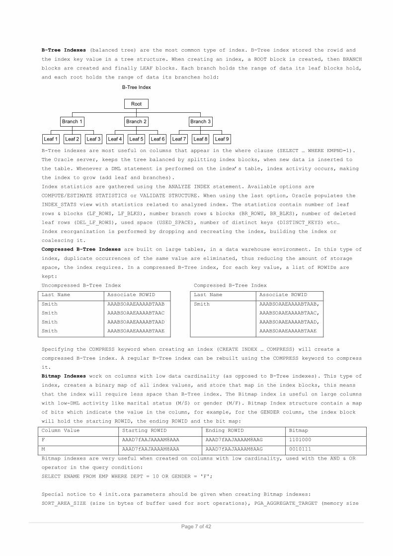
B-Tree Indexes (balanced tree) are the most common type of index. B-Tree index stored the rowid and
the index key value in a tree structure. When creating an index, a ROOT block is created, then BRANCH
blocks are created and finally LEAF blocks. Each branch holds the range of data its leaf blocks hold,
and each root holds the range of data its branches hold:
B-Tree Index
Leaf 1 Leaf 2 Leaf 3
Branch 1
Leaf 4 Leaf 5 Leaf 6
Branch 2
Leaf 7 Leaf 8 Leaf 9
Branch 3
Root
B-Tree indexes are most useful on columns that appear in the where clause (SELECT … WHERE EMPNO=1).
The Oracle server, keeps the tree balanced by splitting index blocks, when new data is inserted to
the table. Whenever a DML statement is performed on the index’s table, index activity occurs, making
the index to grow (add leaf and branches).
Index statistics are gathered using the ANALYZE INDEX statement. Available options are
COMPUTE/ESTIMATE STATISTICS or VALIDATE STRUCTURE. When using the last option, Oracle populates the
INDEX_STATS view with statistics related to analyzed index. The statistics contain number of leaf
rows & blocks (LF_ROWS, LF_BLKS), number branch rows & blocks (BR_ROWS, BR_BLKS), number of deleted
leaf rows (DEL_LF_ROWS), used space (USED_SPACE), number of distinct keys (DISTINCT_KEYS) etc…
Index reorganization is performed by dropping and recreating the index, building the index or
coalescing it.
Compressed B-Tree Indexes are built on large tables, in a data warehouse environment. In this type of
index, duplicate occurrences of the same value are eliminated, thus reducing the amount of storage
space, the index requires. In a compressed B-Tree index, for each key value, a list of ROWIDs are
kept:
Uncompressed B-Tree Index Compressed B-Tree Index
Last Name Associate ROWID Last Name Associate ROWID
Smith
Smith
Smith
Smith
AAABSOAAEAAAABTAAB
AAABSOAAEAAAABTAAC
AAABSOAAEAAAABTAAD
AAABSOAAEAAAABTAAE
Smith AAABSOAAEAAAABTAAB,
AAABSOAAEAAAABTAAC,
AAABSOAAEAAAABTAAD,
AAABSOAAEAAAABTAAE
Specifying the COMPRESS keyword when creating an index (CREATE INDEX … COMPRESS) will create a
compressed B-Tree index. A regular B-Tree index can be rebuilt using the COMPRESS keyword to compress
it.
Bitmap Indexes work on columns with low data cardinality (as opposed to B-Tree indexes). This type of
index, creates a binary map of all index values, and store that map in the index blocks, this means
that the index will require less space than B-Tree index. The Bitmap index is useful on large columns
with low-DML activity like marital status (M/S) or gender (M/F). Bitmap Index structure contain a map
of bits which indicate the value in the column, for example, for the GENDER column, the index block
will hold the starting ROWID, the ending ROWID and the bit map:
Column Value Starting ROWID Ending ROWID Bitmap
F AAAD7fAAJAAAAM8AAA AAAD7fAAJAAAAM8AAG 1101000
M AAAD7fAAJAAAAM8AAA AAAD7fAAJAAAAM8AAG 0010111
Bitmap indexes are very useful when created on columns with low cardinality, used with the AND & OR
operator in the query condition:
SELECT ENAME FROM EMP WHERE DEPT = 10 OR GENDER = 'F';
Special notice to 4 init.ora parameters should be given when creating Bitmap indexes:
SORT_AREA_SIZE (size in bytes of buffer used for sort operations), PGA_AGGREGATE_TARGET (memory size
Page 7 of 42

in bytes assigned to a bitmap index creation and bitmap merges following index range scan),
CREATE_BITMAP_AREA_SIZE and BITMAP_MERGE_ARE_SIZE were deprecated in 9i and were replaced by
PGA_AGGREGATE_TARGET.
Function-Based Indexes are indexes created on columns that a function is usually applied on. When
using a function on an indexed column, the index is ignored, therefore a function-based index is very
useful for these operations.
Example: UPPER function on ENAME column in EMP table – CREATE INDEX … on EMP(UPPER(ENAME));
or (units * unit_price) calculation in the SALES table: CREATE INDEX … on SALES(units * unit_price);
Reverse-Key Indexes are special types of B-Tree indexes and are very useful when created on columns
contain sequential numbers. When using a regular B-Tree, the index will grow to have many branches
and perhaps several levels, thus causing performance degradation, the RKI solve the problem by
reversing the bytes of each column key and indexing the new data. This method distributes the data
evenly in the index. Creating a RKI is done using the REVERSE keyword: CREATE INDEX … ON … REVERSE;
Index Organized Tables (IOT) – Using B-Tree, Bitmap and RKI indexes are used for tables that store
data in an unordered fashion (Heap Tables). These indexes contain the location of the ROWID of
required table row, thus allowing direct access to row data. In order to store data in a specific
order, Oracle provides the IOT – instead of storing the ROWID pointing to the table row, the whole
row is stored in the index itself. There are 2 benefits of using IOT:
1. table rows are indexes, access to table is done using its primary key, the row is returned quickly
from IOT than heap tables. 2. There is less I/O when using the IOT.
In order to create an IOT, use the CREATE TABLE command:
CREATE TABLE …
ORGANIZATION INDEX TABLESPACE … (specify this is an IOT)
PCTTHRESHOLD … (specify % of block to hold in order to store row data, valid 0-50 (default 50))
INCLUDING … (specify which column to break a row when row length exceeds PCTTHRESHOLD)
OVERFLOW TABLESPACE … (specify the tablespace where the second part of the row will be stored)
MAPPING TABLE; (cause creation of a mapping table, needed when creating Bitmap index on IOT)
The Mapping Table maps the index’s physical ROWIDs to logical ROWIDs in the IOT. IOT use logical
ROWIDs to manage table access by index because physical ROWIDs are changed whenever data is added to
or removed from the table.
In order to distinct the IOT from other indexes, query the USER_INDEXES view using the
pct_direct_access column. Only IOT will have a non-NULL value for this column.
Index information can be obtained from several views such as DBA_INDEXES (column INDEX_TYPE,
COPMRESSION & FUCNIDX_STATUS), DBA_SEGMENTS (column SEGMENT_TYPE) and DBA_TABLES (columns IOT_NAME &
IOT_TYPE).
Identifying unused indexes is done by placing the index in monitoring state using the
ALTER INDEX … MONITORING USAGE command. This action will populate the V$OBJECT_USAGE view that can be
queries to identify object usage. To turn off monitoring use ALTER INDEX … NOMONITORING USAGE;
Partitions – partitions are subsets of data separated physically from one another. The CBO will
benefit greatly from using partitions by skipping irrelevant partitions. There are four types of
partitions: Range partitions, List partitions, Hash partitions and Composite partitions.
Range Partitions represent a partition data division by range of values (date for example). In order
to create a range partitioned table use: CREATE TABLE … PARTITION BY RANGE (column) PARTITION P1
values … TABLESPACE …, PARTITION P2 …. The partition key can be compressed up to 16 columns. A table
can have up to 65536 partitions. Gaps are now allowed in Range partitions (skip of date for example),
all rows stored in a partition will have values less than, and not equal to the upper bound for that
partition. The value specified by LESS_THAN clause must be literal (date, number). Range partitions
cannot contain columns with LONG/LONG RAW data type. Specifying the ENABLE ROW MOVEMENT clause in the
creation of partitions will enable the data to move across partitions.
List Partitions are similar to Range partitions except they are based on a set of specified values
rather than a range of values. List partitions are created using the PARTITION BY LIST (column)
Page 8 of 42
clause and each partition must specify its list of values: CREATE TABLE … PARTITION BY LIST (degree)
(PARTITION P1 VALUES ('BS', 'BA', 'BBA'), PARTITION P2 VALUES ('MS', 'MA', 'MBA');
Hash partitions use a hashing algorithm to assign inserted records into partitions. This has the
effect of maintaining a relatively even number of records in each partition, thus improving the
performance of parallel operations like Parallel Query and Parallel DML. Hash partitions are created
using the PARTITION BY HASH (column) PARTITIONS n clause, where n specifies the number of partitions.
There are several rules regarding Hash partitions: The partition key should have high cardinality
(column should contain unique values or very few duplicate values). Hash partitions work best when
data is retrieved from via the unique key. Range lookups on hash partitioned tables derive no benefit
from the partitioning, When they are properly indexed, hash partitioned tables improve the
performance of joins between two or more partitioned tables. Updates that would cause a record to
move across partition boundaries are not allowed. Local hash indexes can be built on each partition.
Composite Partitioning represents a combination of both range and hash partitioning. This type of
partition is useful when Range partitioning is desired, but when the resulting number of values
within each range would be uneven. Composite partitions are created using:
PARTITION BY RANGE (column 1) SUBPARTITION BY HASH (column 2) SUBPARTITIONS n.
Several guidelines related to composite partitioning should be considered:
The partitions are logical structures only; the table data is physically stored at the sub-partition
level, Composite partitions are useful for historical, date-related queries at the partition level.
Composite partitions are also useful for parallel operations (both query and DML) at the subpartition
level, Partition-wise joins are also supported using composite local indexes, and Global local
indexes are not supported .
Indexing Partitioned Tables - After a partitioned table has been created, it should be indexed.
Proper indexing of partitioned tables will also improve the manageability of the indexes when
performing routine index maintenance tasks. There are two methods of classifying partitioned indexes:
1) Local vs. global indexes - whether the index’s partitioning structure matches that of the
underlying, indexed table. 2) Prefixed vs. non-prefixed indexes - whether the index contains the
partition key and where the partition key appears within the index structure.
Local Partition Indexes are said to be local when the number of partitions in the index match the
underlying table’s partitions on a one-to-one basis. Therefore, if a table contains four partitions,
the local index on that table will also contain four partitions, each indexing one of the four table
partitions. Several guidelines related to local partition indexes:
Local partitioned indexes can use any of the four partition types, Oracle automatically maintains the
relationship between the table’s partitions and the index’s partitions, If a table partition is
merged, split, or dropped, the associated index partition will be merged, split, or dropped, Any
bitmapped index built on a partitioned table must be a local index .
Global Partition Indexes are said to be global when the number of partitions in the index do not
match the underlying table’s partitions on a one-to-one basis. For example, if a table contains four
partitions, its global index may be comprised of only two partitions, each of which may encompass one
or more of the table partitions. Several guidelines related to global partition indexes:
Although global indexes can be built on a range, list, hash, or composite partitioned table, the
global partitioned index itself must be Range partitioned. The highest partition of a global index
must be defined using the MAXVALUE parameter. Performing maintenance operations on partitioned tables
can cause their associated global indexes to be placed into an invalid state. Indexes in an invalid
state must be rebuilt before users can access the table. Creating a global partitioned index with the
same number of partitions as its underlying table (i.e. simulating a local partitioned index) does
not substitute for a local partitioned index. The indexes would not be considered the same by the CBO
despite their similar structures.
Prefixed Partition Indexes are said to be prefixed whenever the left-most column of the index is the
same as the underlying table’s partition key column. For example, if a table were partitioned on the
Page 9 of 42
specific column, a prefixed partitioned index would also use the same column as the first column in
its index definition. Prefixed indexes can be either unique or non-unique.
Non-prefixed Partitioned Indexes are said to be non-prefixed when the left-most column of the index
is not the same as the underlying table’s partition key column. For example, if a table were
partitioned on a specific column, a non-prefixed partitioned index would use some column other than
the one specified as the first column in its index definition.
Combination of Partitioned Indexes:
Local index Global index
Prefixed index Local, prefixed
Partitioned index
Global, prefixed
Partitioned index
Non-prefixed index Local, non-prefixed
Partitioned index
Not Allowed
Creating a Local, Prefixed Partition Index:
CREATE INDEX index_name ON table_name (column_name) LOCAL;
The above syntax would create a partition index with the same number of partitions as the underlying
table whose leading column would be the same column that makes up the underlying table’s partition
key.
Creating a Local, Non-prefixed Partition Index:
CREATE INDEX index_name ON table_name (column_name) LOCAL;
The above syntax would create a partition index with the same number of partitions as the underlying
table whose leading column would be a column different from that, which makes up the underlying
table’s partition key.
Creating a Global, Prefixed Partition Index:
CREATE INDEX index_name ON table_name (column 1) GLOBAL PARTITION BY RANGE (column 1)
(PARTITION P1 VALUES LESS THAN …, PARTITION P2 VALUES LESS THAN…);
The above syntax would create a n-partition index (according to number of partitions defined in the
call). In addition to the above partitioned index types, traditional non-partitioned B-Tree indexes
can also be built on partitioned tables. These indexes are referred to as global, prefixed non-
partitioned indexes.
How the Partitioned Tables Affect the Optimizer - Once partitioned tables and indexes have been
created, it is up to the cost-based optimizer to decide how to use them effectively when executing
application queries. Because the Oracle9i CBO is very 'partition aware', it can eliminate partitions
that will not be part of the query result. Partitioned tables and indexes also help the CBO develop
effective execution plans by influencing the manner in which joins are performed between two or more
partitioned tables. When performed in parallel using Oracle Parallel Query, there are two possible
join methods that are considered by the CBO: full partition-wise joins and partial partition-wise
joins. Partition-wise joins occur any time two tables are joined on their partition key columns.
Partition-wise joins can be performed either serially or in parallel. Partial partition-wise joins
occur any time two tables are joined on the partition key columns of one of the two tables. Partial
partition-wise joins can only be performed in parallel. Each of these join types reduces the overall
CPU and memory utilized to service a query, particularly on very large partitioned tables.
Partition information can be gathered with the help of these views: DBA_IND_PARTITIONS (details about
index partitions), DBA_LOB_PARTITIONS (details about large object partitions),
DBA_PART_COL_STATISTICS (columns statistics for partitioned tables), DBA_PART_HISTOGRAMS (histogram
statistics for partitioned tables), DBA_PART_INDEXES (details about partitioned index),
DBA_PART_KEY_COLUMNS (partition key columns for all partitioned tables and indexes), DBA_PART_LOBS
(details about each partitioned large object), DBA_PART_TABLES (details about each partitioned
table), DBA_TAB_PARTITIONS (details about each table’s individual partitions).
For each DBA view of partitions, exists an exact view for the Sub Partition.
Page 10 of 42
Index and Hash Clusters - A cluster is a group of one or more tables whose data is stored together in
the same data blocks. In this way, queries that utilize these tables via a table join don’t have to
read two sets of data blocks to get their results; they only have to read one. There are two types of
clusters available in Oracle9i: the Index cluster and the Hash cluster.
Index Clusters are used to store the data from one or more tables in the same physical Oracle blocks.
Clustered tables should have these attributes: Always be queried together and only infrequently on
their own, Have little or no DML activity performed on them after the initial load and have roughly
equal numbers of child records for each parent key. A cluster is a segment stored in a tablespace.
The cluster is accessed via an index that contains entries that point to the specific key values on
which the tables are joined. In order to create a cluster, use CREATE CLUSTER cluster_name
(column_name data_type) SIZE n STORAGE … TABLESPACE …; command. The parameter SIZE specifies how many
cluster keys to have per Oracle block (db_block_size/SIZE).
Hash Clusters are used in place of a traditional index to quickly find rows stored in a table. Like
cluster indexes. Hash cluster tables should have these attributes: Have little or no DML activity
performed on them after the initial load, have a uniform distribution of values in the indexed
column, have a predictable number of values in the indexed column and be queried with SQL statements
that utilize equality matches against the indexed column in their WHERE clauses.
Rather than examine an index and then retrieve the rows from a table, a Hash cluster’s data is stored
so queries against the cluster can use a hashing algorithm to determine directly where a row is
stored with no intervening index required.
OLTP vs. DSS Tuning Requirements
Tuning OLTP Systems
Online Transaction Processing (OLTP) systems tend to be accessed by large numbers of users doing
short DML transactions. Users of OLTP systems are primarily concerned with throughput.
OLTP systems need enough B-Tree and Reverse Key indexes to meet performance goals but not so many as
to slow down the performance of INSERT, UPDATE, and DELETE activity. Bitmap indexes are not a good
choice for OLTP systems because of the locking issues they can cause. Table and index statistics
should be gathered regularly if the CBO is used because data volumes tend to change quickly in OLTP
systems. OLTP indexes should also be rebuilt frequently if the data in the tables they are indexing
is frequently modified.
Tuning DSS Systems
Decision Support Systems (DSS) and data warehouses represent the other end of the tuning spectrum.
These systems tend to have very little if any DML activity, except when data is mass loaded or purged
at the end of a period. Users of these systems are concerned with response time, which is the time it
takes to get the results from their queries. DSS makes heavy use of full table scans so the
appropriate use of indexes and Hash clusters are important. Index-organized tables can also be
important tuning options for large DSS systems. Bitmap indexes may be considered where the column
data has low cardinality but is frequently used as the basis for queries. Thought should also be
given to selecting the appropriate optimizer mode and gathering new statistics whenever data is
loaded or purged. The use of histograms may also help improve DSS response time. Finally,
consideration should be given to database block size, init.ora parameters related to sorting, and the
possible use of the Oracle Parallel Query option. As with OLTP systems, database statistics should
also be gathered following each data load if the CBO is used.
Tuning Hybrid Systems: OLTP and DSS
Some systems are a combination of both OLTP and DSS. These hybrid systems can present a significant
challenge because the tuning options that help one type of system frequently hinder the other.
However, through the careful use of indexing and resource management, some level of coexistence can
usually be achieved. As the demands on each of these systems grows, you will probably ultimately have
to split the two types of systems into two separate environments in order to meet the needs of both
user communities.
Page 11 of 42

4 – Tuning the Shared Pool
• The Shared Pool is the portion of the SGA that caches the recently issued SQL and PL/SQL statements.
The Shared Pool is managed by a Least Recently Used (LRU) algorithm. Once the Shared Pool is full,
this algorithm makes room for subsequent SQL statements by aging out the statements that have been
least recently accessed. By caching these frequently used statements in memory, an application that
issues the same SQL or PL/SQL statement benefits from the fact that the statement is already in
memory, ready to be executed. This is very useful for the subsequent application calls as the user
can skip some of the overhead that was incurred when the statement was originally issued.
Benefits or Statement Caching – When a user executes a query, the Oracle server converts the query
into a string of ASCII characters. The ASCII string is then passed through a hashing algorithm, which
generates a hash value. Next, the Server Process checks to see if the hashed value is already exists
in the shared pool. If is exists, the Server Process uses the cached version of the statement to
execute it. If the hashed value does not exist in the shared pool the statement is parsed and then
executed. The parse step must complete the following tasks:
1. Check statement for syntax errors
2. Perform object resolution (check names and structures of referenced objects in data dictionary)
3. Gather statistics regarding the objects referenced in the query in the data dictionary
4. Prepare and select an execution plan, check for stored outlines or materialized views
5. Determine the security for the objects referenced in the query by examining the data dictionary
6. Generate a compiled version of the statement (called P-Code)
The parsing process is expensive and therefore must not be avoided by making sure that most SQL
Statements find a parsed version of themselves in the shared pool. Finding a matching SQL statement
in the Shared Pool is referred to as a cache hit. Not finding a matching statement and having to
perform the parse operation is considered a cache miss. In order for a cache hit to occur, the two
SQL statements must match exactly; the ASCII equivalents of the two statements must be identical for
them to hash to the same value in the Shared Pool. Maximizing cache hits and minimizing cache misses
is the goal of all Shared Pool tuning. As of Oracle9i, a hashed value is also assigned to the
execution plan for each cached SQL statement.
Components of the Shared Pool – the shared pool is made of three components:
Library Cache – All SQL and PL/SQL statements are cached in the library cache. The statements can be
procedures, functions, triggers, anonymous PL/SQL blocks or java classes. The cached statement
contains several components: statement text, the hashed value, the P-Code, statistics and execution
plan. SQL-Related Dynamic Performance Views: V$SQL - SQL statement text and statistics for all cached
SQL statements including I/O, memory usage, and execution frequency, V$SQLAREA - information for SQL
statements that are cached in memory, parsed, and ready for execution, V$SQLTEXT - The complete text
of the cached SQL statements along with a classification by command type and V$SQL_PLAN - Execution
plan information for each cached SQL statement. The V$SESSION COMMAND column, displays the types of
SQL a user is issuing: 2-Insert, 3-Select, 6-Update, 7-Delete, 26-Lock table, 44-Commit, 45-Rollback
and 47-PL/SQL Execute. The V$DB_OBJECT_CACHE displays the types of database objects that are being
referenced by the application’s SQL statements. The EXECUTIONS column displays how often the
application SQL has referenced the database object.
Data Dictionary Cache - data dictionary cache stored the structure of the tables, columns and data
types referenced in the statement. It also stores the issuing user’s privileges on the objects
involved. This memory area is also managed using an LRU mechanism. When data dictionary information
is kept in memory, subsequent application users who issue similar, but not identical, statements as
previous users, benefit from the fact that the data dictionary information associated with the tables
in their statement may be in memory—even if the actual statement is not.
User Global Area - The UGA is only present in the Shared Pool if the Shared Server option is being
used. In the shared server architecture, the User Global Area is used to cache application user
session information. In a dedicated server environment, session information is maintained in the
application user’s private Process Global Area (PGA).
Page 12 of 42
Measuring the Performance of the Shared Pool - The primary indicator of the performance of the Shared
Pool is the cache-hit ratio. High cache-hit ratios indicate users are frequently finding the SQL and
PL/SQL statements they are issuing already in memory. Hit ratios can be calculated for both the
Library Cache and the Data Dictionary Cache. Oracle recommends tuning the Library Cache first, before
attempting to tune the Database Buffer Cache.
Measuring Library Cache Performance – The library cache performance is measured by calculating the
hit ratio. There are 4 places to get library cache hit ratio: V$LIBRARYCACHE view, UTLBSTAT/ESTAT,
STATSPACK and Oracle Performance Manager GUI tool.
V$LIBRARYCACHE view, displays information about cache hit ratio. The GETHITRATIO column shows cache
hit ratio related to the parse phase, the PINHITRATIO column shows cache hit ratio related to
execution phase. Other useful columns for Library Cache tuning are INVALIDATION, which display the
number of times a cached SQL statement was marked as invalid and therefore forced to parse Cached
statements are marked invalid whenever the objects they reference are modified and RELOADS, which
shows the number of times that an statement had to be re-parsed because the Library Cache had aged
out or invalidated. The NAMESPACE column shows the source of the cached object (BODY, CLUSTER, INDEX,
JAVA DATA, JAVA RESOURCE, JAVA SOURCE, OBJECT, SQL AREA, TABLE/PROCEDURE, TRIGGER).
GETHITRATIO - Oracle uses the term get to refer to a type of lock, called a Parse Lock, that is taken
out on an object during the parse phase for the statement that references that object. Each time a
statement is parsed, the value for GETS in the V$LIBRARYCACHE view is incremented by 1.
The GETHIT column stores the number of times a statement found its parsed copy in memory.
PINHITRATIO - PINS, like GETS, are also related to locking. However, PINS are related to locks that
occur at execution time. These locks are the short-term locks used when accessing an object.
Therefore, each library cache GET also requires an associated PIN, in either Shared or Exclusive
mode, before accessing the statement’s referenced objects. Each time a statement is executed, the
value for PINS is incremented by 1. The PINHITRATIO column stored the number of times a statement
found the associated parsed SQL Library Cache.
Measuring Data Dictionary Cache Performance - Like the Library Cache, the measure of the
effectiveness of the Data Dictionary Cache is expressed in terms of a hit ratio. This Dictionary
Cache hit ratio shows how frequently the application finds the data dictionary information it needs
in memory, instead of having to read it from disk. This hit-ratio information is contained in a
dynamic performance view called V$ROWCACHE. Querying GETS and GETMISSES columns in V$ROWCACHE, can be
used to calculate the Data Dictionary Cache hit ratio. The output from STATSPACK and REPORT.TXT also
contain statistics related to the Data Dictionary Cache hit ratio.
Improving Shared Pool Performance - The objective of all these methods is to increase Shared Pool
performance by improving Library Cache and Data Dictionary Cache hit ratios. These techniques fall
into five categories: Make it bigger, Make room for large PL/SQL statements, Keep important PL/SQL
code in memory, Encourage code reuse and Tune Library Cache–specific init.ora parameters.
Make it Bigger - The simplest way to improve the performance of the Library and Data Dictionary
Caches is to increase the size of the Shared Pool. Because the Oracle Server dynamically manages the
relative sizes of the Library and Data Dictionary Caches, making the Shared Pool larger lessens the
likelihood that cached information will be moved out of either cache by the LRU mechanism. This has
the effect of improving both the Library Cache and Data Dictionary Cache hit ratios.
The shared pool size is determined by the SHARED_POOL_SIZE init.ora parameter (default 64M for 64-bit
operating systems and 16M for 32-bit operating systems). If java is installed in the Oracle server,
the shared pool must be at least 50M in size (it is possible to configure the java pool for this
purpose by setting the JAVA_POOL_SIZE parameter in the init.ora parameter file). Shared pool size can
be increased dynamically using the ALTER SYSTEM SET SHARED_POOL_SIZE command (increase size allowed
until SGA_MAX_SIZE is reached).
Make room for large PL/SQL statements - If an application makes a call to a large PL/SQL package or
trigger, several other cached SQL statements may be moved out of memory by the LRU mechanism when
this large package is loaded into the Library Cache. This has the effect of reducing the Library
Page 13 of 42
Cache hit ratio if these statements are subsequently re-read into memory later. To avoid this
problem, Oracle gives you the ability to set aside a portion of the Library Cache for use by large
PL/SQL packages. This area of the Shared Pool is called the Shared Pool Reserved Area. The init.ora
parameter SHARED_POOL_RESERVED_SIZE can be used to set aside a portion of the Shared Pool for
exclusive use by large PL/SQL packages and triggers. The value of SHARED_POOL_RESERVED_SIZE is
specified in bytes and can be set to any value up to 50 percent of the value specified by
SHARED_POOL_SIZE. By default, SHARED_POOL_RESERVEDSIZE will be 5 percent of the size of the Shared
Pool. Oracle recommends setting SHARED_POOL_RESERVED_SIZE to 10 percent of the SHARED_POOL_SIZE. A
way to determine the optimal size of your reserve pool is to monitor the V$DB_OBJECT_CACHE dynamic
performance view. The V$SHARED_POOL_RESERVED view can be used to monitor the use of the Shared Pool
Reserved Area and help determine if it is properly sized. If you have over-allocated memory for the
reserved area, you should notice that the REQUEST_MISSES column are consistently zero or static,
FREE_SPACE column shoes more than 50 percent of the total size allocated to the reserved area. The
REQUEST_FAILURES column indicates that the reserved area is too small if Non-zero or steadily
increasing values appear. Oracle recommends that you aim to have REQUEST_MISSES and REQUEST_FAILURES
near zero in V$SHARED_POOL_RESERVED when using the Shared Pool Reserved Area.
The ABORTED_REQUEST_THRESHOLD procedure in the DBMS_SHARED_POOL package is used to specify how much
of the Library Cache’s memory can be flushed from the Shared Pool’s LRU list when a large PL/SQL
object is trying to find space for itself in memory.
Keep Important PL/SQL Code in Memory - Applications that make heavy use of PL/SQL packages and
triggers or Oracle sequences can improve their Shared Pool hit ratios by permanently caching these
frequently used PL/SQL objects in memory until the instance is shutdown. This process is known as
pinning and is accomplished by using the DBMS_SHARED_POOL package. Pinned packages are stored in the
Shared Pool Reserved Area. ALTER SYSTEM FLUSH SHARED_POOL does not flush pinned objects. However,
pinned objects will be removed from memory at the next instance shutdown.
DBMS_SHARED_POOL package is created by running the $ORACLE_HOME/rdbms/admin/dbmspool.sql script. By
using the KEEP procedure, the object specified as the parameter for the procedure is pinned in the
shared pool. The V$DB_OBJECT_CACHE view contains the KEPT column which indicates the pinned objects.
What to Pin – The most used objects such as triggers, packages, procedures, etc…
When to Pin - Right after instance startup. This is accomplished by manually executing SQL script
after instance startup, or automatically by an AFTER STARTUP ON DATABASE trigger.
Encourage Code Reuse – Adopt coding standards in order to increase shared pool performance or use
bind variables.
Tune Library Cache–specific init.ora Parameters - In addition to SHARED_POOL_SIZE, there are three
init.ora parameters that directly affect the performance on the Library Cache:
OPEN_CURSORS - The parameter limits the number of cursors a user’s session can open (default 50).
Increasing this value will allow each user to open more cursors and minimize re-parsing previously
executed SQL statements, thus improving the Library Cache hit ratio.
CURSOR_SPACE_FOR_TIME - When set to TRUE, shared SQL areas are pinned in the Shared Pool (default
FALSE). This prevents the LRU from removing a shared SQL area from memory unless all cursors that
reference that shared SQL area are closed. This can improve the Library Cache hit ratio and reduce
SQL execution time. Set to TRUE only if you have enough server memory to make the Shared Pool large
enough to hold all the potential pinned SQL areas.
SESSION_CACHED_CURSORS - the parameter specified how many of the cursors associated with SQL
statements, which have been issued several times, should be cached in the Library Cache (default 0).
CURSOR_SHARING - The parameter allows you to change the Shared Pool’s default behavior when parsing
and caching SQL statements. Values for CURSOR_SHARING Parameter:
FORCE - Allows two SQL statements, which differ only by a literal value, to share parsed code cached
in the Shared Pool.
SIMILAR - Allows two SQL statements, which differ only by a literal value, to share parsed code
cached in the Shared Pool.
Page 14 of 42

EXACT Two SQL statements must match exactly in order to share the parsed code cached in the Shared
Pool (default).
5 - Tuning the Database Buffer Cache
• The Database Buffer Cache or Buffer Cache is the portion of the SGA that caches copies of the most
recently used data blocks. Each buffer in the Buffer Cache holds the contents of, one database block.
The blocks cached in the Buffer Cache may belong to any of the following segment types: Tables,
Indexes, Clusters, LOB segments, LOB indexes, Rollback segments and Temporary segments.
The usage of these buffers in the Database Buffer Cache is managed by a combination of mechanisms:
LRU list - When a SQL statement is issued, the data associated with that statement will be copied
from disk into the Buffer Cache in the SGA. Each Server Process is responsible for copying this data
from the datafiles into the buffers in the Buffer Cache. The Database Buffer Cache is managed by a
Least Recently Used (LRU) algorithm. Once the Buffer Cache’s buffers are full, the LRU algorithm
makes room for subsequent requests for new buffers by aging out the buffers that have been least
recently accessed .This allows the Oracle Server to keep the most recently requested data buffers in
the Buffer Cache while the less commonly used data buffers are flushed. By caching the data buffers
in this manner, Statements which need the same data buffers as a previous SQL Statement, benefits
from the fact that the buffers are already in memory and therefore do not need to be read from disk.
When a request is made for data, the user’s
Server Process copies the blocks (A, B, C) from
disk into buffers at the beginning MRU. These
buffers stay on the LRU List but move towards
the LRU end as additional data blocks are read
into memory. If a buffer (A) is accessed again
during the time it is on the LRU List, the
buffer is moved back to the beginning of the
LRU List (back to the MRU). If buffers are not
accessed again before they reach the end of the
LRU List, the buffers (B and C) are marked as
free and will subsequently be overwritten by
another block being read from disk.
The behavior of the LRU List is slightly different when a table is accessed during a full table scan.
During an FTS, the table buffers are placed immediately at the least recently used end of the LRU
List. While this has the effect of immediately causing these blocks to be flushed from the cache, it
also prevents an FTS on a large table from pushing all other buffers out of the cache.
The buffers that the LRU list maintains can be in one of four states:
Free - Buffer is not currently in use.
Pinned - Buffer is currently in use by a Server Process.
Clean - A buffer that was released from a pin and has been marked for immediate reuse.
Dirty - Buffer is not in use, but contains committed data that has not yet been written to disk by
Database Writer.
The mechanism for managing these dirty buffers is called the Dirty List or Write List. Using a
checkpoint queue, this list keeps track of all the blocks that have been modified using INSERT,
DELETE or UPDATE statements, but have not yet been written to disk. Dirty buffers are written to disk
by the Database Writer (DBW0). Each Server Process also makes use of the Dirty List while carrying
out its Buffer Cache–related activities.
User Server Process – When the Server Process does not find the data it needs in the Buffer Cache, it
must read the data from disk. Before the data can be read from disk, however, a free buffer must be
Page 15 of 42
found to hold the copy of the data block in memory. When searching for a free buffer to hold the
block, the Server Process makes use of both the LRU List and the Dirty List:
While searching the LRU List for a free block, the Server Process moves any dirty blocks it finds on
the LRU List to the Dirty List. As buffers are added to the Dirty List, it grows longer and longer.
When it hits a predetermined threshold length, DBW0 writes the dirty buffers to disk. DBW0 also write
dirty buffers to disk when a Server Process has examined too many buffers without successfully
finding a free buffer. In this case, DBW0 will write dirty buffers directly from the LRU List (as
opposed to moving them to the Dirty List first, as above) to disk. When a Server Process needs a
buffer and finds that buffer in memory, the buffer may contain uncommitted data or data that has
changed since the time the user’s transaction began. Since uncommitted data is not displayed to user,
the Server Process uses a buffer that contains the before image of the data to provide a read
consistent view of the database. This before-image is stored in a rollback segment whose blocks are
also cached in the Buffer Cache. The Database Writer background process also directly assists in the
management of the LRU and Dirty Lists.
Database Writer - Several database events cause Database Writer to write the dirty buffers to disk:
Dirty List threshold is reached, LRU List is searched too long without finding a free buffer, Every
three seconds, At Checkpoint, At Database Shutdown (Unless a SHUTDOWN ABORT is used), At Tablespace
Offline Temporary and At Drop Segment (index or table).
Measuring the Performance of the Database Buffer Cache - Like the Shared Pool, one indicator of the
performance of the Database Buffer Cache is the cache hit ratio. Cache hits occur whenever a SQL
statement finds user finds a data buffer needed, in memory. Cache misses occur when the user does not
find the requested data in memory, causing the data to be read from disk.
Buffer Cache hit ratio information can be found at:
V$SYSSTAT – contains statistics regarding overall system performance, gathered since instance
startup. Contains these columns: STATISTIC# - The identifier of the performance statistic, NAME - The
name of the performance statistic, CLASS - The category the statistic falls into (1=User, 2=Redo,
4=Enqueue, 8=Cache, 16=Operating System, 32=Real Application Cluster, 64=SQL, 128=Debug) and VALUE -
The value currently associated with this statistic.
There are only four statistics associated with performance of the Database Buffer Cache:
Physical Reads - number of data blocks (i.e., tables, indexes, and rollback segments) read from disk
into the Buffer Cache since instance startup.
Physical Reads Direct - number of reads that bypassed the Buffer Cache, because the data blocks were
read directly from disk instead (i.e.: Parallel Query).
Physical Reads Direct (LOB) - number of reads that bypassed the Buffer Cache, because the data blocks
were associated with a Large Object (LOB) datatype.
Session Logical Reads - number of times a request for a data block was satisfied by using a buffer
cached in the Database Buffer cache. For read consistency, some of these buffers may have contained
data from rollback segments.
STATSPACK output - The STATSPACK utility output, contains a calculation for the Database Buffer Cache
hit ratio under the Instance Efficiency Percentages section, in the Buffer Hit category.
UTLBSTAT.SQL/UTLESTAT.SQL output - The REPORT.TXT contains a section that shows the statistics needed
to calculate the Database Buffer Cache hit ratio. These statistics include the Physical Reads,
Physical Reads Direct, Physical Reads Direct (LOB) and Session Logical.
Non–Hit Ratio Performance Measures - there are non–hit ratio measures of Buffer Cache effectiveness:
Free Buffer Inspected - number of Buffer Cache buffers inspected by the Server Processes before
finding a free buffer. A closely related statistic is dirty buffer inspected, which represents the
total number of dirty buffers a user process found while trying to find a free buffer.
Free Buffer Waits - number of waits experienced by the Server Processes during Free Buffer Inspected
activity. These waits occur whenever the Server Process had to wait for Database Writer to write a
dirty buffer to disk.
Page 16 of 42

Buffer Busy Waits - number of times the Server Processes waited for a free buffer to become
available. These waits occur whenever a buffer requested by a Server Processes, is already in memory,
but is in use by another process. These waits can occur for rollback segment buffers as well as data
and index buffers.
High or steadily increasing values for any of these statistics, indicate that Server Processes are
spending too much time searching for and waiting for access to free buffers in the Database Buffer
Cache. V$SYSSTAT view contains statistics on the Free Buffer Inspected statistic and the
V$SYSTEM_EVENT view contains statistics on the Free Buffer Waits and Buffer Busy Waits.
Improving Buffer Cache Performance - The objective of these methods is to increase Database Buffer
Cache performance by improving its hit ratio. These techniques fall into five categories:
• Make it bigger – The easiest way to improve Database Buffer Cache performance is to increase its
size. The larger the Database Buffer Cache, the less likely cached buffers are to be moved out of
the cache by the LRU List. The longer buffers are stored in the Database Buffer Cache, the higher
the hit ratio will be. Increasing the size of the Buffer Cache will also lower the number of
waits reported by the free buffer inspected, buffer busy waits, and free buffer waits system
statistics.
In Oracle9i, Database Buffer Cache size is determined by several init.ora parameters:
DB_BLOCK_SIZE - Defines the primary block size for the database.
DB_CACHE_SIZE - Determines the size of the Default Buffer Pool (default 48M).
DB_KEEP_CACHE_SIZE - Determines the size of the Keep Buffer Cache (default 0KB).
DB_RECYCLE_CACHE_SIZE - Determines the size of the Recycle Buffer Cache (default 0KB).
DB_nK_CACHE_SIZE - Specifies the size of the Buffer Cache for segments with nKB block size. Valid
values are 2,4,8,16,32.
In order to improve performance, the Buffer Cache can be divided into up to three different areas
called the Default, Keep, and Recycle. By default, only the Default Pool is configured, as both
the Recycle and Keep Pool are assigned zero bytes.
The size of the Database Buffer Cache and its three component pools can all be changed
dynamically using the ALTER SYSTEM command. Three rules must be kept in mind:
1) The size specified must be a multiple of the granule size
2) The total size of the Buffer Cache, Shared Pool, and Redo Log Buffer cannot exceed the value
specified by SGA_MAX_SIZE
3) The Default Pool cannot be set to a size of zero.
Oracle9i Buffer Cache Advisory displays the performance changes that might occur if the Buffer
Cache were made larger (or smaller) than its existing size.
Using the Buffer Cache Advisory feature requires some initial configuration.
Configuring the Buffer Cache Advisory Feature - You must set the init.ora parameter
DB_CACHE_ADVICE = ON in order for the Buffer Cache Advisory feature to gather statistics about
how changes to the Buffer Cache size might affect performance. Setting this parameter to ON
causes Oracle9i to allocate memory to the Buffer Cache Advisory feature and causes the Buffer
Cache Advisory feature to start gathering statistics about the Buffer Cache’s performance.
Other possible values for the DB_CACHE_ADVICE parameter are: OFF - Turns off the Buffer Cache
Advisory feature and releases any memory or CPU resources allocated to it. READY - Pre-allocates
memory to the Buffer Cache Advisory process, but does not actually start it. Therefore, no CPU is
consumed and no statistics are gathered until the DB_CACHE_ADVICE parameter is set to ON.
The V$DB_CACHE_ADVICE view contains information gathered by the Buffer Cache Advisory:
ID - identifier for the Buffer Pool being referenced. Can be a value from 1 to 8, NAME - name of
the Buffer Pool being referenced, BLOCK_SIZE - block size for the buffers in this Buffer Pool,
shown in bytes, ADVICE_STATUS - status of the Buffer Cache Advisory feature (i.e. OFF, READY,
ON), SIZE_FOR_ESTIMATE - cache size estimate used when predicting the number of physicals reads,
expressed in MB, BUFFERS_FOR_ESTIMATE - cache size estimate used when predicting the number of
physicals reads, expressed in buffers, ESTD_PHYSICAL_READ_FACTOR - ratio comparing the estimated
Page 17 of 42
number of physical reads to the actual number of reads that occurred against the current cache,
NULL if no physical reads occurred, ESTD_PHYSICAL_READS - estimated number of physical reads that
would have occurred if the cache size specified by SIZE_FOR_ESTIMATE and BUFFER_FOR_ESTIMATE had
actually been used for the DB_CACHE_SIZE.
• Use multiple Buffer Pools – By default, all database segments compete for use of the same
Database Buffer Cache buffers in the Default Pool. This can lead to a situation where some
infrequently accessed tables push more-frequently-used data buffers out of memory. To avoid this,
Oracle provides you with the ability to divide the Database Buffer Cache into three separate
areas called Buffer Pools. Segments are then explicitly assigned to use the appropriate Buffer
Pool as determined by the DBA: Keep Pool - Used to cache segments that you rarely, if ever, want
to leave the Database Buffer Cache. The size of this pool is designated by the init.ora parameter
DB_KEEP_CACHE_SIZE. The use of the Keep Pool is optional (default 0 byte). Recycle Pool - Used to
cache segments that you rarely want to retain in the Database Buffer Cache. The size of a Recycle
Pool is designated by the init.ora parameter DB_RECYCLE_CACHE_SIZE. The use of a Recycle Pool is
also optional (default 0 bytes). Default Pool - The size of this pool is designated by the
DB_CACHE_ SIZE init.ora parameter. The Default Pool is required (default 48Mb). This parameter
cannot be set to zero.
Determining Which Segments to Cache - Four views, V$BH, DBA_OBJECTS, V$CACHE, and DBA_USERS can
be used for this purpose. The V$BH and DBA_OBJECTS views contain useful information that can help
you identify which segments are currently cached in the Buffer Cache. V$CACHE and DBA_USERS can
give additional information about segments that might make good candidates for caching in the
Keep or Recycle Pools.
Determining the Size of Each Pool - After determining which segments you wish to cache, you need
to determine how large each pool should be. Making this determination is easy if the segments to
be cached have been analyzed. The BLOCKS column of the DBA_TABLES and DBA_INDEXES data dictionary
views can be used to determine how many Database Buffer Cache buffers would be needed to cache an
entire segment or portion of that segment.
Assigning Segments to Pools – Assigning segments to pools is done using the ALTER TABLE
table_name STORAGE (BUFFER_POOL KEEP/RECYCLE).
Monitoring the Performance of Multiple Buffer Pools – The V$BUFFER_POOL view contains information
about the configuration of the multiple Buffer Pools themselves. The V$BUFFER_POOL_STATISTICS
view contains several columns that contain information that is useful for calculating hit ratios
for each of the individual Buffer Pools (DB_BLOCK_GETS - number of requests for segment data that
were satisfied by using cached segment buffers, CONSISTENT_GETS - umber of requests for segment
data that were satisfied by using cached rollback blocks for read consistency, PHYSICAL_READS –
number of requests for segment data that required that the data be read from disk into the Buffer
Cache)
• Cache tables in memory – Each Buffer Pool is managed by an LRU List. As was noted earlier, tables
that are accessed via a full table scan (FTS) place their blocks immediately at the least
recently used end of the LRU List. If table is accessed again via FTS, the blocks are re-read
from disk to memory. One way to manage this problem, particularly with small tables, is to make
use of cached tables . Cached table buffers are placed at the most recently used end of the LRU
List just as if they had not been full table scanned. This has the effect of keeping these
buffers in memory longer while still accessing them in the most efficient manner. Cached tables
can be implemented in three ways: at table creation (CREATE TABLE ... STORAGE ... CACHE;), by
altering the table after creation (ALTER TABLE table_name CACHE;) or by using a hint in SQL
statement (SELECT /*+ CACHE */ … from …). Displaying Cache Table Information - You can use the
CACHE column in the DBA_TABLES view to determine which tables are cached.
• Bypass the Buffer Cache – By bypassing the Buffer Cache, buffers that are already stored there
are not moved down or off the LRU List during processing. These two types of transactions can be
Page 18 of 42
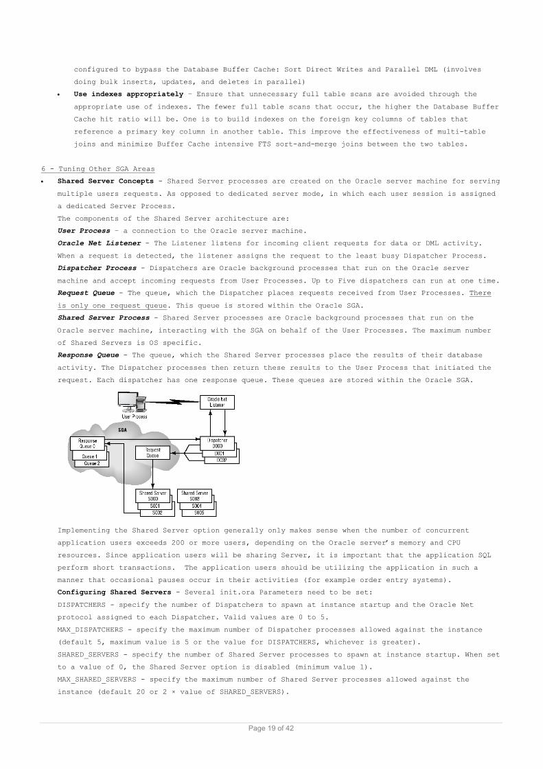
configured to bypass the Database Buffer Cache: Sort Direct Writes and Parallel DML (involves
doing bulk inserts, updates, and deletes in parallel)
• Use indexes appropriately – Ensure that unnecessary full table scans are avoided through the
appropriate use of indexes. The fewer full table scans that occur, the higher the Database Buffer
Cache hit ratio will be. One is to build indexes on the foreign key columns of tables that
reference a primary key column in another table. This improve the effectiveness of multi-table
joins and minimize Buffer Cache intensive FTS sort-and-merge joins between the two tables.
6 - Tuning Other SGA Areas
• Shared Server Concepts - Shared Server processes are created on the Oracle server machine for serving
multiple users requests. As opposed to dedicated server mode, in which each user session is assigned
a dedicated Server Process.
The components of the Shared Server architecture are:
User Process – a connection to the Oracle server machine.
Oracle Net Listener - The Listener listens for incoming client requests for data or DML activity.
When a request is detected, the listener assigns the request to the least busy Dispatcher Process.
Dispatcher Process - Dispatchers are Oracle background processes that run on the Oracle server
machine and accept incoming requests from User Processes. Up to Five dispatchers can run at one time.
Request Queue - The queue, which the Dispatcher places requests received from User Processes. There
is only one request queue. This queue is stored within the Oracle SGA.
Shared Server Process - Shared Server processes are Oracle background processes that run on the
Oracle server machine, interacting with the SGA on behalf of the User Processes. The maximum number
of Shared Servers is OS specific.
Response Queue - The queue, which the Shared Server processes place the results of their database
activity. The Dispatcher processes then return these results to the User Process that initiated the
request. Each dispatcher has one response queue. These queues are stored within the Oracle SGA.
Implementing the Shared Server option generally only makes sense when the number of concurrent
application users exceeds 200 or more users, depending on the Oracle server’s memory and CPU
resources. Since application users will be sharing Server, it is important that the application SQL
perform short transactions. The application users should be utilizing the application in such a
manner that occasional pauses occur in their activities (for example order entry systems).
Configuring Shared Servers - Several init.ora Parameters need to be set:
DISPATCHERS - specify the number of Dispatchers to spawn at instance startup and the Oracle Net
protocol assigned to each Dispatcher. Valid values are 0 to 5.
MAX_DISPATCHERS - specify the maximum number of Dispatcher processes allowed against the instance
(default 5, maximum value is 5 or the value for DISPATCHERS, whichever is greater).
SHARED_SERVERS - specify the number of Shared Server processes to spawn at instance startup. When set
to a value of 0, the Shared Server option is disabled (minimum value 1).
MAX_SHARED_SERVERS - specify the maximum number of Shared Server processes allowed against the
instance (default 20 or 2 × value of SHARED_SERVERS).
Page 19 of 42

CIRCUITS - specify the number of virtual circuits for handling incoming and outgoing network
connections.
PROCESSES - specify the maximum number of OS processes that can access the instance.
DISPATCHERS and SHARED_SERVERS parameters are used to specify the number of Dispatchers and Shared
Server process to spawn at instance startup. While Dispatcher processes must be explicitly started by
the DBA using the ALTER SYSTEM command, Shared Server processes can be dynamically started and
stopped by the PMON background process based on the demands placed on those resources by the
connected application users.
Measuring Shared Server Performance – Several view contain Shared Server Information:
V$SHARED_SERVER view contains detailed statistics about the Shared Server processes, including idle
and busy times for each Shared Server process.
V$QUEUE view contains information about contention for Shared Server Request and Response queues.
V$SHARED_SERVER_MONITOR view contains statistics regarding the Shared Server processes, including the
Shared Servers that have been dynamically started and terminated by PMON since instance startup.
V$DISPATCHER view contains detailed statistics about the Shared Server Dispatcher processes,
including idle and busy times for each Dispatcher process.
V$DISPATCHER_RATE view contains historical and real-time statistics regarding Dispatcher activity.
V$CIRCUIT view contains statistics about the path, or circuit, a User Process has taken through a
Dispatcher, Request Queue, Shared Server, Response Queue, and back to the User Process again.
Monitoring Shared Server Process Performance – can be obtained through monitoring the rate the
available server processes are servicing database requests. This busy ratio can be calculated using
the V$SHARED_SERVER view (NAME - Shared Server process name, REQUESTS - Total number of requests that
the Shared Server has serviced during the time it was running, BUSY - Total amount of time (in 100ths
of a second) that the Shared Server was busy during the time it was running, IDLE - Total amount of
time (in 100ths of a second) that the Shared Server was idle during the time it was running).
When User Processes make a database request, their requests are initially placed in the Request Queue
by the Dispatcher process. If there are too few Shared Server processes, these requests may
experience a delay while waiting to be serviced. These waits for access to a Shared Server process
can be monitored using the V$QUEUE view (TYPE - queue type (DISPATCHER, COMMON), TOTALQ - number of
items placed in the queue, WAIT - total time spent waiting for access to a Shared Server process, in
100ths of second).
Monitoring Dispatcher Performance - The performance of the Dispatcher processes can also be monitored
using a "busy ratio". This ratio can be calculated using the V$DISPATCHER view using the following
columns: NETWORK - protocol used by the Dispatcher (network address), STATUS - current status of the
Dispatcher (WAIT (idle), SEND (sending a message), RECEIVE (receiving a message), CONNECT
(establishing connection), DISCONNECT (disconnecting a session), BREAK (performing a break),
TERMINATE (terminating a connection), ACCEPT (accepting connections), REFUSE (refusing connection)),
OWNED - number of virtual circuits owned by this Dispatcher, BUSY - total time (in 100ths of second)
that the Dispatcher was busy, IDLE Total time (in 100ths of second) that the Dispatcher was idle.
Another indication of Shared Server performance is the amount of time that User Processes are waiting
to have their requests accepted by the Dispatchers. The V$QUEUE and V$DISPATCHER dynamic performance
views can be used to calculate the average wait.
The waits indicated by the V$QUEUE and V$DISPATCHER views are a sign of Dispatcher contention.
Additional evidence that contention for Dispatchers is occurring in the Shared Server environment can
be determined by querying the V$DISPATCHER_RATE (NAME - Dispatcher name, CUR_IN_CONNECT_RATE -
current Dispatcher service request rate, MAX_IN_CONNECT_RATE - maximum Dispatcher service request
rate).
The V$SHARED_SERVER_MONITOR view gives an overview of the cumulative activity of the Shared Server
environment. This view contains five columns:
MAXIMUM_CONNECTIONS - maximum number of virtual circuits used by Shared Servers since instance
startup. MAXIMUM_SESSIONS - maximum number of Shared Server sessions that have been utilized since
Page 20 of 42

instance startup. SERVERS_STARTED - number of additional Shared Servers, which were automatically
started since instance startup (beyond the number of Shared Servers specified by the SHARED_SERVERS
init.ora parameter). SERVERS_TERMINATED - Total number of Shared Servers that were automatically shut
down by the Shared Server option since the instance was started. SERVERS_HIGHWATER - maximum number
of Shared Servers running since the instance was started (both those that were started explicitly in
the init.ora and those started implicitly by PMON).
Improving Shared Server Performance - Performance problems with the Shared Server architecture are
usually related to one of the following areas: SGA components are not adequately sized for the Shared
Server environment, Too few Shared Servers running to adequately service user requests, Too few
Dispatchers are running to adequately service user requests.
Increase the Size of Related SGA Components – In shared server environment, the user session and
cursor state information (e.g., bind variable values and session settings) resides inside the Shared
Pool in the SGA under the Shared Server configuration, Thus forcing the DBA to increase the Shared
Pool size.
Increasing the Number of Shared Servers - Whenever Shared Servers are unable to service the incoming
requests, the PMON background process will dynamically start additional Shared Server processes, up
to the limit specified by the MAX_SHARED_SERVERS value in init.ora. You can also explicitly add
additional Shared Server processes either dynamically or manually:
Dynamically Adding Additional Shared Servers - by using the ALTER SYSTEM SET shared_servers = n;
Manually Adding Additional Shared Servers – by increasing the value for SHARED_SERVERS in the
init.ora (requires instance restart).
Increasing the Number of Dispatchers - Dispatcher processes are not dynamically started. Additional
Dispatchers can be added dynamically or manually:
Dynamically Adding Additional Dispatchers - by using ALTER SYSTEM SET dispatchers = 'protocol, n';
(protocol – the network protocol (i.e. TCP), n – number of dispatchers).
Manually Adding Additional Dispatchers - by increasing the value for DISPATCHERS in the init.ora
(requires instance restart).
Large Pool Concepts
The Large Pool is an optional SGA structure, which can be used to process requests for optional
features like Recovery Manager and Parallel Query.
Configuring the Large Pool - The LARGE_POOL_SIZE parameter defines the size of the Large Pool
(default 0 unless PARALLEL_AUTOMATIC_TUNING parameter is set to TRUE, in which case the size of the
Large Pool is set automatically). Once configured, the Large Pool’s memory area can be used to cache
data related to: I/O slave processes for Database Writer, Backup and restore operations for Recovery
Manager, Shared Server session data, Messaging information for the Parallel Query option.
When configuring the Large Pool manually, the minimum value allowed for LARGE_POOL_SIZE is 600K.
Measuring the Performance of the Large Pool - V$SGASTAT view displays how much space is allocated to
the Large Pool (using POOL column).
Improving the Performance of the Large Pool - Large Pool size can be increases by sizing the value
for LARGE_POOL_SIZE in the init.ora. The range of values for LARGE_POOL_SIZE is 600K to 2GB or more
depending on operating system. The value of LARGE_POOL_SIZE cannot be changed dynamically using the
ALTER SYSTEM command.
Java Pool Concepts
Oracle9i allows you to dedicate a portion of the SGA, called the Java Pool, as the location where
session-specific Java code and application variables reside during program execution. Configuring the
java pool correctly is critical to the successful performance of any Java-based Oracle application.
Configuring the Oracle Java Environment - The primary parameter is JAVA_POOL_SIZE, which is used to
set the size of the SGA memory structure where most Java-related session data is cached during
execution. SHARED_POOL_SIZE - Shared Pool memory is used by the JVM when Java classes are loaded and
compiled and when Java resources in the database are accessed. JAVA_POOL_SIZE - All other Java-
related session data is cached in the Java Pool memory structure (default 20M; valid values 1M-1G).
Page 21 of 42
JAVA_SOFT_SESSIONSPACE_LIMIT - When memory is allocated to a Java process, the amount of memory
requested is compared to this limit. If the request exceeds this limit, a message is written to a
user trace file in the USER_DUMP_ DEST (default 0; maximum value 4GB). JAVA_MAX_SESSIONSPACE_SIZE -
When memory is allocated to a Java process, the amount of memory requested is compared to this limit.
If the request exceeds this limit, an out-of memory error (ORA-29554) occurs (default 0; maximum 4GB)
Measuring the Performance of the Java Pool - monitor java pool using V$SGASTAT (POOL column),
STATSPACK output (performance of the Java Pool - java free memory).
Improving the Performance of the Java Pool - you can increase the size of the Java Pool by increasing
the value for JAVA_POOL_SIZE in init.ora. The range of values for JAVA_POOL_SIZE is 1M to 1GB. The
size of the Java Pool cannot be changed dynamically.
7 - Tuning Redo Mechanisms
• Oracle’s redo mechanisms record the changes made to data so committed transactions can be 'redone' in
the event of a server failure or user error. Oracle’s redo mechanisms consist of five components:
Redo Log Buffer – A portion of the SGA, which records the information needed to redo transactions in
the event of media failure or user error. These transactions may be DML statements as INSERT, UPDATE
or DELETE, or DDL statements like CREATE, ALTER or DROP. Redo information is copied into the Redo Log
Buffer by each user’s Server Process.
Log Writer (LGWR) – A background process, which is responsible for writing the contents on the Redo
Log Buffer to the Online Redo Logs. Each instance has only one Log Writer.
Database Checkpoints - A checkpoint event represents the moment in time when the database is in a
consistent state. Checkpoints are important because, following instance failure, only those
transactions that occurred after the last checkpoint have to be recovered during instance recovery.
Online Redo Logs – A background process, which writes the contents of the Redo Log Buffer to physical
files called Redo Logs. Every database must have a minimum of at least two Redo Log files. When LGWR
fills the current Redo Log with redo information, LGWR switches to the next Redo Log group before
writing the next batch of redo information.
Archived Redo Logs - After LGWR has written to all the available Online Redo Logs, LGWR will start
over by writing to the first Redo Log group again. If the data in this Redo Log is not preserved
somehow, the redo information contained in the log will be lost, limiting your ability to perform a
complete database recovery. However, a database operating in Archive Log Mode will not reuse an
Online Redo Log until the Archiver (ARC0) background process has copied the contents of the log to
the archive destination.
Tuning the Redo Log Buffer - The Redo Log Buffer’s management mechanism can be thought of as funnel,
where transaction redo information enters at the top of the funnel and is then occasionally emptied
out the bottom of the funnel by the LGWR background process. To keep up with the volume of incoming
Redo Log Buffer entries, LGWR is prompted to write the contents of the Redo Log Buffer to disk
whenever any of the following events occur: a COMMIT command is issued, every three seconds, the Redo
Log Buffer is 1/3 full, Redo Log Buffer reaches 1MB and Whenever a database checkpoint occurs.
The size of the Redo Log Buffer is determined by the LOG_BUFFER parameter.
Measuring the Performance of the Redo Log Buffer - Performance is measured by the of the number and
length of waits Server Processes experience when trying to place entries in the Redo Log Buffer.
These waits can be viewed in the V$SYSSTAT and V$SESSION_WAIT views, STATSPACK output and
UTLBSTAT/ESTAT output (REPORT.TXT).
Using V$SYSSTAT to Measure Redo Log Buffer Performance – V$SYSSTAT contains 3 relevant statistics:
redo buffer allocation retries - refers to the number of times a Server Process had to wait and then
retry placing their entries in the Redo Log Buffer because LGWR had not yet written the current
entries to the Online Redo Log.
redo entries - reports the number of entries that have been placed into the Redo Log Buffer by the
user Server Processes since instance startup.
redo log space requests - measures how often LGWR is waiting for a Redo Log switch to occur when
Page 22 of 42
moving from the current Online Redo Log to the next.
During a Redo Log switch, LGWR cannot empty the contents of the Redo Log Buffer. This may cause user
Server Processes to experience a wait when trying to access the Redo Log Buffer. This wait generates
a retry request. Therefore, high or increasing values for redo log space requests indicate that your
Redo Logs may be too small. This can also indicate a problem with I/O contention.
Using V$SESSION_WAIT to Measure Redo Log Buffer Performance - V$SESSION_WAIT shows how long, and for
which events, individual user sessions have waited. STATE column in V$SESSION_WAIT valid values:
WAITING - The session is waiting at that moment, WAITED UNKNOWN TIME - Duration of the last wait is
undetermined, WAITED SHORT TIME - The last wait lasted less than 1/100th of a second and WAITED KNOWN
TIME - The value in the WAIT_TIME column is the actual wait time.
Using STATSPACK Output to Measure Redo Log Buffer Performance - Redo Log Buffer performance
information appears in two different sections of the STATSPACK output file:
Instance Efficiency Percentages - indicates the Redo Log Buffer performance in terms of a ratio
called the Redo NoWait% (percentage of time that user Server Processes did not experience a wait when
attempting to place an entry in the Redo Log).
Instance Activity Stats - - contains the same statistical information found in the V$SYSSTAT dynamic
performance view.
Using REPORT.TXT Output to Measure Redo Log Buffer Performance - contains a section that shows the
same statistics related to Redo Log Buffer performance that are found in V$SYSSTAT and STATSPACK
output.
Improving Redo Log Buffer Performance - The objective of Redo Log Buffer tuning is to make sure that
user Server Processes have access to, and can place entries in, the Redo Log Buffer without
experiencing a wait. These techniques fall into two categories:
Make It Bigger - The larger the Redo Log Buffer is, the less likely user Server Processes are to
experience a wait when trying to place redo entries into the buffer. The size of the Redo Log Buffer
is specified in bytes using LOG_BUFFER parameter (default 512KB, or 128KB × the number of CPUs
whichever is greater). The range of values is 64K to an OS specific maximum. An acceptable tuning
practice is to continue increasing the size of the Redo Log Buffer until the Redo Log Buffer Retry
Ratio shows no further improvement or the value for the statistic log buffer space in V$SESSION_WAIT
ceases to diminish.
Reduce redo generation - This technique is implemented using one of the following methods:
UNRECOVERABLE - this keyword is used when creating a table using the CREATE TABLE AS SELECT.
Tables created in this manner do not generate any redo information for the inserts generated by the
CREATE statement’s sub-query. However, any subsequent DML on the table will generate entries in the
Redo Log Buffer. By default, all tables created using the CREATE TABLE AS SELECT are recoverable.
NOLOGGING - Like UNRECOVERABLE, the NOLOGGING option also allows you to specify, which tables should
skip generating redo entries for certain types of DML. However, unlike UNRECOVERABLE, NOLOGGING is an
attribute of the table that stays in effect until you disable it. You can specify the NOLOGGING
attribute at either table creation, or after creation using the ALTER TABLE statement. Once the
NOLOGGING attribute is set on a table, redo entry generation will be suppressed for all subsequent
DML on the table only when that DML is of the following types: Direct Path loads using SQL*Loader or
Direct load inserts using the /*+ APPEND */ hint. In addition to the CREATE TABLE and ALTER TABLE,
the following commands can also be used with the NOLOGGING: CREATE TABLE AS SELECT, CREATE INDEX,
ALTER INDEX REBUILD and CREATE TABLESPACE.
Tuning Checkpoints - A checkpoint event represents the moment in time when the database is in a
consistent state. Checkpoints are important because, if instance failure occurs, only transactions
that occurred after the last checkpoint have to be recovered.
There are two types of checkpoints: incremental and full.
When an incremental checkpoint occurs, the following actions take place:
The CKPT updates the control file headers immediately with then SCN and the Redo Log sequence.
When a full checkpoint event occurs, the following actions occur in the database:
Page 23 of 42
DBW0 writes all buffers in the Buffer Cache containing committed transactions to disk.
LGWR writes all the contents of the Redo Log Buffer to the Online Redo Log files.
The CKPT updates the control file headers.
Database checkpoints occur whenever the instance is shutdown (except ABORT), the Online Redo Log
switches from the current log to the next, the DBA issues the ALTER SYSTEM CHECKPOINT command, when a
tablespace is placed into hot backup mode using the ALTER TABLESPACE … BEGIN BACKUP command or when a
tablespace is taken offline. (This checkpoint is a special form of the complete checkpoint referred
to as a full tablespace checkpoint. During this type of checkpoint, only the dirty buffers belonging
to the tablespace in hot backup mode are written to disk) and when the value specified by the
init.ora parameter FAST_START_MTTR_TARGET is exceeded.
Measuring the Performance of Checkpoints - It is important to monitor checkpoint activity because too
many checkpoints causes unnecessary I/O and too few checkpoints exposes the database to longer
instance recovery times. Checkpoint performance information can be gathered from V$SYSTEM_EVENT and
V$SYSSTAT views, STATSPACK, REPORT.TXT, the Alert log and the OEM Performance Manager.
Using V$SYSTEM_EVENT to Measure Checkpoint Performance - Occasionally, checkpoint events are started,
but do not complete successfully because a second checkpoint request occurs very soon after the
first. You can detect checkpoints that are started but not completed by querying the checkpoint
incomplete statistic in V$SYSTEM_EVENT. This view reports the number of waits that have occurred
since instance startup for a variety of events and contains these columns:
EVENT - name of the event associated with the wait, TOTAL_WAITS - total number of times a wait
occurred for this event & AVERAGE_WAIT - The average time, in 100ths of a second, spent waiting for
this event.
Two events found in the V$SYSTEM_EVENT view, are indicators of checkpoint performance:
Checkpoint Completed - This event shows how often waits occurred for the checkpoint to complete its
activities. High or steadily increasing values for this event indicate that checkpoints need to be
tuned.
Log File Switch (Checkpoint Incomplete) - This event shows how often the Online Redo Log switched
from one log to the next, before the checkpoint from the previous log switch had time to complete.
When this occurs, the in-progress checkpoint is abandoned and a new checkpoint is begun. (Because
incomplete checkpoints cause excess I/O that do not provide any recovery benefits, checkpoint
activity should be tuned).
Another indicator can be found in the V$SYSSTAT view. Two statistics, background checkpoints started
and background checkpoints completed, can be used to determine whether all the checkpoints that were
started, actually completed.
Using STATSPACK and REPORT.TXT to Measure Checkpoint Performance - The output in both files, show the
background checkpoints started and background checkpoints completed events.
Using the Alert Log to Measure Checkpoint Performance - The Alert log records the Redo Logs switches
and shows if they are switching too fast and not allowing enough time for a checkpoint that has been
started to complete normally. In this case the 'Checkpoint not complete' message will appear.
Using Performance Manager to Measure Checkpoint Performance - The Performance Manager component of
OEM can also monitor the performance of checkpoint activity. The Average Dirty Queue Length option
of the Performance Manager I/O feature indicates how often checkpoint activity is occurring.
Improving Checkpoint Performance - The techniques for tuning database checkpoint activity fall into
two categories:
Make it bigger - increase the size of the Redo Logs. Since checkpoints occur at every log switch
increasing the redo logs size will reduce the number of checkpoints. Since Redo Logs cannot be
altered to a larger size, the only way to increase their size is to add new logs with a larger size,
and then drop the original, smaller logs.
Adjust checkpoint-related init.ora parameters - Checkpoint has two purposes: assure that all buffers
in the Database Buffer Cache that contain committed transactions are written to disk and limit
instance recovery time by recording that fact in the headers of the datafiles and control files.
Page 24 of 42
Using FAST_START_MTTR_TARGET, you can specify a mean time (in seconds) to recover the instance
following an instance failure (Valid values are 0-3,600 seconds). Oracle will perform additional
checkpoints, beyond the ones performed at a log switch, in order to ensure that the checkpoints are
happening frequently enough to meet the recovery target. If FAST_START_IO_TARGET and
LOG_CHECKPOINT_INTERVAL parameter are used, the FAST_START_MTTR_TARGET parameter is ignored.
V$INSTANCE_RECOVERY view helps monitor the FAST_START_MTTR_TARGET effectiveness. The view contains
these columns: TARGET_MTTR - the target Mean Time to Recover and ESTIMATED_MTTR - the estimated mean
time to recover the instance if it were to fail at that moment.
Similar information can be retrieved from STATSPACK output under Instance Recovery Stats section.
Tuning Online Redo Log Files - Tuning Redo Log performance is critical to ensure not only optimal
performance, but also optimal recovery.
Measuring the Performance of Redo Logs - V$SYSTEM_EVENT view and OS utilities can be useful when
monitoring Redo Log performance.
Using V$SYSTEM_EVENT to Measure Redo Log Performance – The view shows statistics on two related
events: log file switch completion - this event indicates the amount of time that LGWR waited for a
log switch to complete. log file parallel write – this event indicates how long it took for LGWR to
write the redo entries from the Redo Log Buffer to the Online Redo Logs.
High or increasing values for both events can indicate Redo Logs contention.
Using OS Utilities to Measure Redo Log Performance - OS utilities often help monitor I/O activity on
disk devices. The Unix utilities sar and iostat are both useful for monitoring disk I/O on the
devices where Redo Logs are located.
Improving Redo Log Performance - is done through applying two rules:
Minimizing Redo Log Contention - separate redo logs from other database files (like Datafiles,
Control Files, and Archive Logs) and Maximizing Redo Log Throughput - place redo logs on the fastest
devices available. Placing the Redo Logs on fast devices will allow LGWR to perform its writes as
quickly as possible.
Tuning Archiving Operations - a primary bottleneck for the Redo Log Buffer performance is the
frequency and efficiency with which the archive background process (ARC0) copies the contents of the
Redo Log files to the archive destination when the database is operating in archive log mode.
If LGWR needs to write to a Redo Log that is currently being archived by ARC0, LGWR will wait until
ARC0 finishes copying the Redo Log’s contents to the archive destination .
To reduce the likelihood of this occurrence, LGWR will automatically start additional archive
background processes (ARC1, ARC2, etc.) when demands on the system warrant them. However, two areas
related to the archiving process can also cause performance problems:
The archive destination fills with archived logs, causing database processing to halt until
additional space is made available.
The ARC0 background process does not keep up with the Redo Log switching activity, causing a wait to
occur when the Redo Logs wrap before ARC0 has completed archiving the contents of the log. These
events can be monitored using the V$ARCHIVE_DEST, V$ARCHIVE_PROCESSES, and V$SYSTEM_EVENT views.
LOG_ARCHIVE_DEST or LOG_ARCHIVE_DEST_n (n in 1-10) parameters specify the location of the archived
Redo Log. When the archive destination becomes full, the database processing halts. The database will
remain halted until space is made available in the archive location or archiving is moved to another
location using ALTER SYSTEM ARCHIVE LOG ALL TO 'location'.
ARC0 Processes Causing Waits at Log Switch - If the Redo Logs are filling and switching too
frequently, LGWR may wrap around and try to write to a Redo Log that has not yet been archived by
ARC0. The LGWR will hang for a moment until the Redo Log has been archived and becomes available. To
prevent this, LGWR automatically starts new Archive processes. The DBA can also start additional
Archiver processes at instance startup by setting the LOG_ARCHIVE_MAX_PROCESSES parameter to a value
between 2 and 10 (1 is the default). V$ARCHIVE_PROCESSES view shows the status of each Archiver
process and whether it is currently busy or idle.
Page 25 of 42
Improving the Performance of Archiving -
Add More - Every Oracle database must have at least two Redo Log groups. By adding additional Redo
Log groups to your database, you decrease the likelihood that LGWR will wait for archiving to end.
Make it Bigger - In addition, increasing the redo logs size can also cut down on the frequency of log
switches. Oracle recommends that a log switch take place approximately every 20 to 30 minutes.
Several init.ora parameters ensure the database will no halt due to filled archive location:
LOG_ARCHIVE_DUPLEX_DEST - By setting this parameter, ARC0 is instructed to write archived Redo Logs
to both locations. When used in conjunction with LOG_ARCHIVE_MIN_SUCCEED_DEST, ARC0 can continue to
archive Redo Log files even if one of the two locations is full.
LOG_ARCHIVE_DEST_n - By setting this parameter, ARC0 is instructed to write archived Redo Logs to
multiple locations. These locations can be local or remote.
LOG_ARCHIVE_MIN_SUCCEED_DEST - When used with LOG_ARCHIVE_DUPLEX_DEST and LOG_ARCHIVE_DEST_n, this
parameter specifies the number of locations to which ARC0 must be able to successfully write archive
log files before an error is raised (default 1, valid values are 1 or 2 for LOG_ARCHIVE_DUPLEX_DEST,
or between 1-5 when used with LOG_ARCHIVE_DEST_n).
LOG_ARCHIVE_DEST_STATE_n - is specified for each corresponding LOG_ARCHIVE_DEST_n parameter and its
valid values are ENABLE or DEFER.
Create Additional ARC0 Processes - LGWR starts additional Archiver processes the current number does
not meet the instance’s archiving needs. Additional Archiver processes are started by using the
LOG_ARCHIVE_MAX_PROCESSES parameter in the init.ora. The number of Archiver processes to start is
somewhat dependent upon the number of archive destinations you have specified and the speed of the
devices that are behind those locations (default 1).
The V$ARCHIVE_PROCESSES view shows the number and activity of multiple Archiver processes and contain
these columns: PROCESS - Identifies which of the 10 Archiver processes the statistics are associated
with. STATUS - Archiver process status. Valid values are STOPPED, SCHEDULED, STARTING, ACTIVE,
STOPPING, TERMINATED. LOG_SEQUENCE - The Redo Log sequence number that is currently being archived.
STAT - current state of the Archiver process (IDLE or BUSY).
8 - Tuning Disk I/O
• Nearly every action that occurs in the database will result in some type of I/O activity. That I/O
activity can either be logical (in memory) or physical (on disk). All of the following activities can
be the source of disk I/Os: Database Writer (DBW0) writing data buffers from the Database Buffer
Cache to the database’s Datafiles. DBW0 writing data to rollback segment blocks to maintain read
consistency. Server Processes reading data blocks into the Database Buffer Cache. Log Writer (LGWR)
writing transaction recovery information from the Redo Log Buffer to the online redo log. Archiver
(ARC0) reading the contents of Redo Logs and writing those contents to the archive destination.
Application user activity temporarily writing large sort requests to disk.
The goals when tuning physical I/O are generally these: Minimize physical I/O by properly sizing the
SGA and perform any remaining physical I/O as fast as possible when it is required.
Tuning Tablespace and Datafile I/O - Every database segment is stored within a logical structure
called a Tablespace. Every database has at least one tablespace, SYSTEM, which is used to store the
Oracle data dictionary tables and indexes. Several tablespaces will be created later for application
data and index data. Temporary tablespace will be created also and will be used for sort operations.
Undo tablespace is required also for the use of undo segments.
Each tablespace is comprised of one or more physical files called Datafiles. The actual I/O occurs
against the Datafiles, therefore, the number and location of the physical Datafiles are an important
area of tuning consideration. In particular, try to minimize disk contention by placing Datafiles for
the various tablespaces on different disk drives, volume groups, or disk controllers in order to
maximize I/O performance.
Measuring Datafile I/O - can be done using the V$FILESTAT and V$DATAFILE views, the output from
STATSPACK, REPORT.TXT and the output from the OEM Performance Manager GUI tool.
Page 26 of 42
Using V$FILESTAT, V$DATAFILE, and V$TEMPFILE to Measure Datafile I/O - these views can be used to
monitor the performance of the read and write activity against the individual Datafiles and
tablespaces in the database. V$FILESTAT view contains these columns: FILE# - The Datafile’s internal
identifier, PHYRDS number of physical reads, PHYWRTS - number of physical writes, AVGIOTIM -
average time, in milliseconds, spent performing I/O, MINIOTIM - minimum time, in milliseconds, spent
performing I/O, MAXIOWTM - maximum time, in milliseconds, spent writing to that Datafile, MAXIORTM -
maximum time, in milliseconds, spent reading from that Datafile.
V$DATAFILE view contains these columns: FILE# - The Datafile’s internal identifier, NAME - the fully
qualified path and name of the Datafile. V$TEMPFILE view contains these columns: FILE# - The
Datafile’s internal identifier, NAME - the fully qualified path and name of the Datafile.
Using STATSPACK and REPORT.TXT to Measure Datafile I/O – The STATSPACK report contains tablespace I/O
statistics under the Tablespace IO Stats section. The REPORT.TXT reports the sum of IO operations
over tablespaces.
Using Performance Manager to Measure Datafile I/O - The Performance Manager component of the Oracle
Enterprise Manager Diagnostics Pack includes several graphical representations of Datafile I/O
performance.
Improving Datafile I/O - Once statistics about Datafile I/O have been gathered, there are several
techniques to enhance the performance of each disk I/O related to Datafiles:
Minimizing Non-Oracle I/O - Do not place non-Oracle files on the same disk drives or logical volumes
as the Datafiles. Placing non-Oracle files on the same disk as the Datafiles may cause contention for
those disk resources.
Using Locally Managed Tablespaces - Locally Managed Tablespace (LMT) uses a bitmap stored in the
header of each of the tablespace’s Datafiles instead of using Free Lists in the data dictionary to
manage the allocation of space within the tablespace. This allows LMTs to allocate and de-allocate
space from the tablespace more quickly, without having to access the data dictionary in the SYSTEM
tablespace.
Balancing Datafile I/O - Allocate storage for segments to the appropriate tablespaces. Excessive I/O
on the SYSTEM tablespace Datafiles can indicate that non-data dictionary segments may be stored in
the SYSTEM tablespace.
The separation of temporary segment and rollback segment tablespaces from the SYSTEM tablespace is
important for both tuning and management purposes, as is separating application tables from their
associated indexes. This technique helps improve performance on busy OLTP systems when tables and
their associated indexes are having their blocks read while the blocks are also having rows inserted
into them. Segregating segments by functional area or size is also important. Redo Logs and Control
Files should be separated from Datafiles too, because their I/O characteristics are different:
Control Files - The Database Writer and Checkpoint background processes write to the Control Files.
The Archiver background process reads from the Control Files during a database recovery. Since
Control Files I/Os are brief, they can be placed almost anywhere without impacting performance.
Datafiles - The DBW0 process writes to Datafiles. The Server Processes reads Datafiles. Separating
System, temporary, and rollback segment Datafiles from application table and index Datafiles will
help enhance performance.
Redo Logs and Archived Redo Logs - Redo Logs are written to in a sequential fashion by the LGWR
process. Redo Logs are also read by the ARC0 process during archiving. Archived Redo Logs are written
to by the ARC0 at a log switch. Datafiles should be separated from Redo Logs not only for recovery
purposes, but also because Datafile I/O is generally random whereas Redo Log I/O is sequential. Redo
Logs and the archived Redo Logs should not be placed on the same device.
Background and User Trace Files - Background and user trace files are written to the directories
specified by BACKGROUND_DUMP_DEST and USER_DUMP_DEST parameters. Trace files can be generated by any
of the Oracle background processes and by user Server Processes. Since these I/Os tend to be very
short, these files haves a negligible impact on performance.
Page 27 of 42
Performing Datafile I/O Quickly to Improve Performance - Performing Datafile I/O quickly is achieved
in three ways:
Placing high I/O Datafiles on separate disk drives and controllers: I/O performance can be improved
by ensuring that several devices are used to store several Datafiles and that these devices are
attached to several separate disk controllers.
Datafile Striping - When a Datafile is striped, it is stored across several devices, not just one.
This increases I/O performance because multiple sets of disk drive heads are brought into use when a
read or write of the Datafile is required. The easiest way to stripe a Datafile is to store the
Datafile on a RAID device (Redundant Array of Independent Disks, consists of several physical disks
that can be managed and accessed as if they were one or more physical devices). Datafiles can also be
manually striped across devices in the absence of a RAID array. Manual striping is accomplished by
creating a tablespace made up of several Datafiles, where each Datafile is placed on a separate
physical device. Next, a segment is created. In order to strip the segment’s extents across the
datafiles, you can use ALTER TABLE table_name ALLOCATE EXTENT (DATAFILE 'file_name' SIZE nK/M).
Tuning DB_FILE_MULTIBLOCK_READ_COUNT – This parameter, determines the maximum number of database
blocks that are read in one I/O operation by a Server Process whenever a full table scan is performed
(default 8). The maximum value for this parameter varies by OS. By increasing this parameter, more
blocks are accessed with each I/O, thereby cutting down on the total I/Os required to scan an entire
table. V$SYSSTAT view holds the table scans (long tables) statistic, which shoes the number of Full
Table Scans that occurred since instance startup. Another view useful for monitoring full table scan
operations is the V$SESSION_LONGOPS view, which shows activity associated with selected long-running
operations like snapshot refreshes, recovery operations, and parallel query jobs.
Tuning DBW0 Performance - DBW0 is responsible for writing buffers from the Database Buffer Cache to
the database Datafiles. DBW0 performs this write activity at database checkpoints and when Server
Processes are searching free buffers in the Database Buffer Cache. Tuning Database Writer’s I/O
activity is an important aspect of tuning the database’s overall disk I/O.
Measuring DBW0 I/O - The V$SYSTEM_EVENT and V$SYSSTAT views, STATSPACK output and REPORT.TXT can be
used to determine whether DBW0 is experiencing any difficulty while performing write requests.
Using V$SYSTEM_EVENT to Measure DBW0 Performance – Several events indicate DBW0 I/O performance:
buffer busy waits - indicates that waits are being experienced for buffers in the Database Buffer
Cache, due to inefficient writing of dirty buffers by DBW0.
db file parallel write - indicates DBW0 may be experiencing waits when writing many blocks in
parallel, due to a slow device on which the Datafiles reside, or the fact that DBW0 cannot keep up
with the write requests it is being asked to perform.
free buffer waits - indicate that Server Processes have been experiencing waits when moving dirty
buffers to the Dirty List while searching the LRU for a free buffer.
write complete waits – indicates that user sessions have been experiencing waits for buffers to be
written from the Database Buffer Cache by DBW0.
Using V$SYSSTAT to Measure Database Writer Performance - V$SYSSTAT view is also a good source for
measuring the performance of DBW0:
redo log space requests - indicates that a wait occurred for a redo log to become available following
a log switch. Since log switch is followed by a checkpoint, both DBW0 and LGWR have to write buffers
from the Database Buffer Cache and Redo Log Buffer respectively, before LGWR can start writing to the
next redo log. If DBW0 is not writing fast enough, redo log space requests may result.
DBWR buffers scanned – indicates the total number of buffers in the Database Buffer Cache that were
examined in order to find dirty buffers to write. Since DBW0 performs this action, DBW0 may perform
writes ineffectively if it is busy examining the LRU List for dirty buffers when it is signaled to
write.
DBWR lru scans – indicates the total number of buffers examined in the LRU dirty list.
Page 28 of 42
Using STATSPACK and REPORT.TXT to Measure Database Writer Performance - STATSPACK output and
REPORT.TXT contain wait event information related to Database Writer in the System Activity Stats and
System wide wait event for background processes respectively.
Improving DBW0 I/O - Two init.ora parameters are used to tune the performance of DBW0’s activities:
DBWR_IO_SLAVES - specifies the number of Database Writer slaves to start at startup (default 0).
The naming convention for the DBW0 slave processes on Unix is: ora_i101_PROD, ora_i102_PROD…
Database Writer slave processes are similar to the DBW0 process itself, except they can only perform
write operations. The purpose of these slaves is to simulate asynchronous I/O on systems that only
support synchronous I/O. After configuring the I/O slaves, DBW0 will coordinate assigning I/O
requests to each of the slave processes. If all available slave processes are busy when an I/O
request is made, then DBW0 will spawn additional processes—up to the limit specified by
DBWR_IO_SLAVES parameter. If no I/O slaves are available when a request is made, a wait will result.
Any time Database Writer spawns I/O slave processes, other background process that perform disk I/O
(i.e., LGWR, ARC0 and RMAN) will also have I/O slaves created to support their I/O activities.
Configure and use multiple DBW processors - While DBW0 slaves can help improve I/O performance, they
are not able to perform all the functions of DBW0 (like manage Dirty and LRU Lists). You can start
additional, Database Writer processes using the DB_WRITER_PROCESSES parameter (default 1, maximum
10). Multiple Database Writer processes generally have better throughput than Database Writer I/O
slaves. If the Buffer Cache wait events are strictly related to DBW0 I/O activity, then starting I/O
slaves is appropriate. If the Buffer cache wait events are occurring for activities related to
internal Buffer Cache management (i.e., free buffer waits events), then starting multiple Database
Writer processes to handle those structures would be more suitable.
Tuning Segment I/O - Oracle segments (e.g., tables and indexes) store their data in tablespaces,
which are made up of one or more of physical Datafiles. Each Datafile is in turn made up of
individual database blocks. These blocks store the actual data for each segment and represent the
smallest unit of I/O that can be performed against a Datafile. When a segment is created, it is
allocated a chunk of contiguous blocks, called an extent.
Understanding Oracle Blocks and Extents - In Oracle9i, there are two block sizes to consider:
The first is the Primary Block Size - is set at database creation and is specified in bytes by the
DB_BLOCK_SIZE parameter. The only way to change the primary block size is to re-create the database.
The second is the local block size associated with an individual tablespace during creation using the
BLOCKSIZE keyword. If BLOCKSIZE is omitted at tablespace creation, the tablespace will use the
primary block size.
An extent is a collection of contiguous Oracle blocks. When a segment is created, it will be assigned
at least one extent called the initial extent. When a segment is dropped, its extents are released
back to the tablespace.
Each Oracle block is divided into three sections:
Block header area - store header information about the contents of that block. Header information
includes the transaction slots specified by the INITRANS parameter at table creation, a directory of
the rows that are contained within the block, and other general header information needed to manage
the contents of the block. This block header information generally consumes between 50 to 200 bytes
of the block’s total size.
Reserved space - using PCTFREE, you can specify how much space is reserved in each block for updates.
This value is specified as a percentage of the overall size of the block. Once a block is filled with
data to the level of PCTFREE, the block will no longer accept new inserts, leaving the remaining
space for update operations. The process of removing a block from the list of available blocks is
performed by the table’s Free List. Whenever a Server Process wants to insert a new row into a
segment, it searches the Free List to find the block ID of a block that is available to accept the
insert. If the subsequent insert should cause the block to fill to above the PCTFREE value, the
block is taken off the Free List. A block stays off of the Free List until enough data is deleted so
that the block’s available space falls below that specified by PCTUSED. The default values for
Page 29 of 42
PCTFREE and PCTUSED are 10 percent and 40 percent respectively.
Free space - The remaining space in the segment block is free space that is used to store the row
data for the segment. The number of rows that will fit into each block is dependent upon the size of
the block and the average row length of the data stored in that segment.
Improving Segment I/O - The goal is to minimize the number of blocks that must be accessed in order
to retrieve requested data. Key areas related to improving segment I/O include:
The cost associated with dynamic extent allocation - When all the available extents assigned to a
segment are full, the next insert operation will cause the segment to acquire a new extent. On
traditional dictionary-managed tablespaces, this dynamic allocation of segment extents incurs
undesirable I/O overhead due to queries that Oracle must perform against the data dictionary. One way
to avoid this issue is to use locally managed tablespaces. Another way to avoid dynamic extent
allocation is to identify tables and indexes that are close to needing an additional extent, and then
assigning them additional extents manually using ALTER TABLE table_name ALLOCATE EXTENT.
The performance impact of extent sizing - Larger extent sizes offer slightly better performance than
smaller extents because they are less likely to dynamically extend and can also have all their
locations identified from a single block (called the extent map) stored in the header of the
segment’s first extent. Large extents also perform better during full table scan operations because
fewer I/Os are required to read the extents (when DB_FILE_MULTIBLOCK_READ_COUNT is set properly). The
disadvantages of large extents sizes are the potential for wasted space within tablespaces and the
possibility that there may not be a large enough set of contiguous Oracle blocks available when an
extent is required.
The performance impact of block sizing - The appropriate block size for your system will depend on
your application, OS specifications, and available hardware. Generally, OLTP systems use smaller
block sizes for these reasons: Small blocks provide better performance for random-access nature.
Small blocks reduce block contention, since each block contains fewer rows. Small blocks are better
for storing the small rows (that are common in OLTP systems). However, small block sizes add to
Database Buffer Cache overhead because more blocks must generally be accessed, since each block
stores fewer rows. Conversely, DSS systems use larger block sizes for these reasons: Large blocks
pack more data and index entries into each block. Large blocks favor the sequential I/O common in
most DSS systems. However, larger block sizes also increase the likelihood of block contention and
require larger Database Buffer Cache sizes to accommodate all the buffers required to achieve
acceptable Database Buffer Cache hit ratios.
How row chaining and migration affect performance - Row Chaining occurs when a row that is inserted
into a table exceeds the size of the database block, causing the row to spill over into two or more
blocks. Row chaining is bad for performance because multiple blocks must be read to return a single
row. The only way to fix a chained row is to either decrease the size of the insert or increase the
Oracle block size. Row migration occurs when a previously inserted row is updated with a value larger
than the space available in the block specified by PCTFREE causing the Oracle Server to move (or
migrates) the row to a new block. When migration occurs, a pointer is left at the original location,
which points to the row’s new location in the new block. Row migration is bad for performance because
Oracle must perform at least two I/Os (one on the original block, and one on the block referenced by
the row pointer) in order to return a single row. Row migration can be minimized by setting PCTFREE
to an appropriate value. There are two techniques for determining whether row chaining and/or
migration are occurring in your database: examining the CHAIN_CNT column in DBA_TABLES and the
presence of the table fetch continued row statistic in V$SYSSTAT. This statistic is also found in the
STATSPACK and REPORT.TXT under Instance Activity Stats.
The role of the High Water Mark during full table scans - As a segment uses the database blocks
allocated to its extents, the Oracle Server keeps track of the highest block ID that has ever been
used to store segment data. This block ID is called the High Water Mark (HWM). The HWM is significant
because a Server Process reads all the segment blocks up to the HWM when performing a full table
scan. Since the HWM does not move when rows are deleted from a segment, many empty blocks may end up
Page 30 of 42
being scanned during a full table scan. If the segment is static, the space above the HWM will be
wasted. After using the ANALYZE command, the EMPTY_BLOCKS column in DBA_TABLES will show the number
of blocks that a table has above its HWM. This unused space can be released using the ALTER TABLE
table_name DEALLOCATE UNUSED command or using the DBMS_SPACE.UNUSED_SPACE procedure.
Tuning Sort I/O - Sorting occurs whenever data must be placed in a specified order. A sort can take
place in one of two locations: in memory or on disk. Sorts in memory are the least expensive in terms
of performance. Sorts to disk are the most expensive because of the extra overhead of the disk I/Os.
The primary tuning goal with regard to sorting is to minimize sort activity. The types of SQL
statements that can cause database sorts are: ORDER BY, GROUP BY, SELECT DISTINCT, UNION, INTERSECT,
MINUS, ANALYZE, CREATE INDEX and Joins between tables on non-indexed columns.
The amount of memory reserved for sorts in each Server Process is determined by 4 parameters:
SORT_AREA_SIZE - specify how much memory is reserved for each Server Process should to perform in-
memory sort operations. The default value for SORT_AREA_SIZE is OS-dependent. The minimum size is
equivalent to six Oracle blocks. The maximum size is OS-dependent. The SORT_AREA_SIZE parameter can
be set at instance level (in init.ora or by issuing the ALTER SYSTEM SET SORT_AREA_SIZE=n DEFERRED
command) or at session level (by using the ALTER SESSION SET SORT_AREA_SIZE=n command).
SORT_AREA_RETAINED_SIZE - specify how much memory each Server Process reduces its memory for the
final fetch. The default value is equal to SORT_AREA_SIZE. The minimum size is the equivalent of two
Oracle blocks. The maximum size is limited to the value of SORT_AREA_SIZE.
The parameter can be set in init.ora, by using the ALTER SYSTEM SET SORT_AREA_RETAINED_SIZE=n
DEFERRED command, or by using the ALTER SESSION SET SORT_AREA_RETAINED_SIZE=n command.
PGA_AGGREGRATE_TARGET - this parameter can be used to establish an upper boundary on the maximum
amount of memory that all user processes can consume while performing database activities, including
sorting (default 0). Valid values range from 10MB to 4000GB.
WORKAREA_SIZE_POLICY - used to determine if the overall amount of memory, assigned to all user
processes, is managed explicitly or implicitly. When set to the default value of MANUAL, the size of
each user’s sort area will be equivalent to the value of SORT_AREA_SIZE for all users. When set to a
value of AUTO, Oracle will automatically manage the overall memory allocations so that they do not
exceed the target specified by PGA_AGGREGATE_TARGET.
Measuring Sort I/O - Sort activity can be monitored using the V$SYSSTAT and V$SORT_SEGMENT views,
using the output from STATSPACK and REPORT.TXT, and using the output from the OEM Performance
Manager.
Using V$SYSSTAT to Measure Sort Activity - The V$SYSSTAT dynamic performance view has two statistics,
sorts (memory) and sorts (disk), that can be used to monitor sort user activity.
Using STATSPACK Output and REPORT.TXT to Measure Sort Activity - STATSPACK utility shows similar sort
statistics. These statistics can be found in several areas of the STATSPACK report (under Instance
Efficiency Percentages). REPORT.TXT also contains sort activity information.
Using OEM Performance Manager to Measure Sort Activity - The Performance Manager includes several
graphical representations of sort performance.
Improving Sort I/O - Sort activity can cause excessive I/O when performed in disk instead of memory.
There are several possible methods of improving sort performance, including:
Avoiding SQL statements that cause sorts - minimize the number of sorts being performed by
application code, ad-hoc queries, and DDL activities:
SQL Statement Syntax - use of the UNION ALL operator instead of the UNION operator. Avoid using the
INTERSECT, MINUS, and DISTINCT keywords.
Use Indexes - Indexing columns that are referenced by ORDER BY and GROUP BY clauses in application
SQL statements can minimize unnecessary sorting.
Index Creation Overhead - eliminate the sort that normally occurs during index creation by using the
NOSORT option of the CREATE INDEX command.
Statistics Calculation - Overhead Sorts can occur whenever table and index statistics are gathered.
Consider using the ESTIMATE option instead COMPUTE of when gathering table and index statistics to
Page 31 of 42

minimize the overhead associated with this process. Gather statistics for only columns that are
relevant to the application SQL by using the ANALYZE ... FOR COLUMNS command.
Make It Bigger - minimize the number of sorts that are done to disk by increasing the value of
SORT_AREA_SIZE. While the amount of memory specified by SORT_AREA_SIZE is not allocated to a session
until they initiate a sort, the server’s available memory must be sufficient to accommodate the
user’s sort area while the sort is being processed. If SORT_AREA_SIZE is set to a large value and
many users are sorting simultaneously, the demands placed on the server’s memory may impact
performance until the memory is released when the sorts are complete. Decreasing the size of
SORT_AREA_RETAINED_SIZE when SORT_AREA_SIZE is increased will help minimize the problem of excessive
memory usage related to sorting.
Making proper use of temporary tablespaces - When a Server Process writes a sort chunk to disk, it
writes the data to the user’s temporary tablespace. This tablespace, although it is referred to as
the user’s temporary tablespace, can be either permanent (contain permanent segments like tables and
indexes, as well as multiple temporary sort segments owned by each Server Process) or temporary
(contain only a single temporary segment, that is shared by all users performing sorts to disk).
Dynamic management of individual sort segments is expensive both in terms of I/O and recursive data
dictionary calls. The sort segments in the temporary tablespace are not dropped when the user’s sort
completes. Instead, the first sort operation following instance startup creates a sort segment that
remains in the temporary tablespace for reuse by subsequent users who also perform sorts to disk.
This sort segment will remain in the temporary tablespace until instance shutdown.
Improving the reads related to sort I/O – 2 views allow monitoring on sort segments:
V$SORT_SEGMENT - The view allows you to monitor the size and growth of the sort segment that resides
in the temporary tablespace. The sort segment will grow dynamically as users place demands on it.
V$SORT_USAGE - The view allows you to see which individual users are causing large sorts to disk.
Tuning Rollback Segment I/O - rollback segments play a critical role in every database DML
transaction because they store the before-image of changed data.
The before-image data stored in the rollback segment is used for three important purposes:
It can be used to restore the original state of the data by issuing a ROLLBACK command.
It provides a read-consistent view of the changed data to other users who access the same data prior
a COMMIT command is issued.
It is used during instance recovery to undo uncommitted transactions that were in progress just prior
to an instance failure.
Rollback segments are made up of extents, which are in turn comprised of contiguous Oracle blocks.
Within each rollback segment, Oracle uses the extents in a circular fashion until the rollback
segment is full. Once the rollback segment is full, no new transactions will be assigned to it until
some of the rollback segment space is released by using COMMIT or ROLLBACK commands. A single
rollback segment can store before-images for several different transactions. However, a transaction
writes its before-image information to only one rollback segment. Once a transaction is assigned to a
rollback segment, the transaction never switches to a different rollback segment. If the before-image
of a transaction grows to fill that extent, the transaction will wrap into the adjacent extent.
Unless you ask for a specific rollback segment using the SET TRANSACTION USE ROLLBACK SEGMENT
command, the Oracle Server assigns transactions to rollback segments. The total number of
transactions a rollback segment can handle is dependent on the Oracle block size.
The goals of rollback-segment tuning usually involve the following: Make sure database users always
find a rollback segment to store their transaction before-images without experiencing a wait.
Make sure that database users always get the read-consistent view.
Make sure database rollback segments do not cause unnecessary I/O.
Measuring Rollback Segment I/O - There are four areas that you should monitor when trying to tune the
performance of rollback segments:
Rollback segments header contention - each rollback segment uses a transaction table stored in its
header block to track the transactions that use it. The header block is generally cached in the
Page 32 of 42
Database Buffer Cache so that all users can access it when trying to store their transaction before-
images. On a busy OLTP system, users may experience a wait for access to these rollback segment
header blocks, thereby causing their transaction performance to decline. 'undo segment tx slot'
statistic in V$SYSTEM_EVENT, 'undo header' and 'system undo header' classes in V$WAITSTAT and
V$ROLLSTAT view (columns USN (undo segment number), GETS (number of times a Server Process succeeded
in accessing the rollback segment header) and WAITS (number of times a Server Process needed to
access the rollback segment header and experienced a wait)) indicate rollback segment header block
contention. STATSPACK and REPORT.TXT also show rollback segment header block contention information
at Rollback Segments Stats and buffer busy wait statistic on the rollback segment undo header
respectively.
Rollback segment extent contention - indicate waits occurring for access to the blocks within the
individual extents of each rollback segment. V$WAITSTAT 'undo block' and 'system undo block' classes
display information about RBS extent contention. V$SYSSTAT 'consistent gets' statistic indicates the
number of times rollback segment extent blocks were accessed in the Database Buffer Cache.
Rollback segments extent wrapping - When a transaction’s before-image exceeds the size of the extent
to which it has been allocated, the transaction will wrap into the next extent if it is available.
This dynamic wrapping incurs a small I/O cost and should be avoided if possible.
V$ROLLSTAT WRAPS column shows how often transactions have wrapped from one extent to another since
instance startup. STATSPACK and REPORT.TXT also show rollback segment extent wrapping information
using Wraps column.
Rollback segments dynamic extent allocation - when a transaction’s before-image exceeds the size of
the extent, but cannot wrap to the next extent because there are still active transactions in that
extent, the rollback segment will add a new extent and wrap into that extent instead. This dynamic
extent allocation incurs an I/O cost that should be avoided if possible. 'undo segment extension'
event in V$SYSTEM_EVENT records how long user Server Processes had to wait for rollback segments to
add extents to handle transaction. V$ROLLSTAT view contains the EXTENDS column, which indicates how
often the rollback segment was forced to add extents to support database transaction activity.
STATSPACK show rollback segment dynamic extent using the EXTENDS column. OEM Performance Manager
includes several graphical representations of undo segment performance (like Undo Segment Hit Ratios
and undo wait statistics).
Improving Rollback Segment I/O - undo segment tuning goals are to eliminate contention for rollback
segments, try to minimize rollback segment extending and wrapping, avoid running out of space in undo
segments, and always have rollback data needed for constructing read consistent images for
application users. In order to achieve these objectives, consider these four tuning categories:
Add more rollback segments - add more rollback segments to the database and create them in a new
tablespace, separated from the existing rollback segments.
Make the existing rollback segments bigger - the optimal size of rollback segments varies with the
type of system (i.e. OLTP vs. DSS) and the types of transactions being performed in the database.
INSERT (Low Cost) UPDATE (Medium Cost) and DELETE (High Cost). By joining the V$SESSION and
V$TRANSACTION views you can see how much space each session is using in the database rollback
segments. Query V$ROLLSTAT view to determine how much rollback segment space the transaction needs.
V$ROLLSTAT's WRITES column, shows how many bytes of before-image data have been written to the
rollback segment.
Explicitly manage rollback segments for large transactions - Very large transactions, like batch
processing runs, require large rollback segments. In these cases, it is best to create one or two
large rollback segments and dedicate them to this purpose.
Minimize the need for rollback space - try to minimize the number and size of entries that are
written to the rollback segments by performing frequent commits to minimize large rollback entries,
using the COMMIT=Y option when performing database imports, forgoing the use of the CONSISTENT option
when using the database EXPORT utility, and setting an appropriate COMMIT value when using the
SQL*Loader utility.
Page 33 of 42
Use automatic undo management features - Oracle9i offers a new feature, Automatic Undo Management
(AUM). Automatic Undo Management is designed to minimize undo segment performance problems by
dynamically managing the size and number of undo segments. With AUM, dedicated tablespaces, called
Undo Tablespaces, are created to hold before-image data. The number and size of these undo segments
is automatically managed by Oracle based on the demands of the system.
Configuring Automatic Undo Management – set UNDO_MANAGEMENT parameter to AUTO (default MANUAL). Set
the UNDO_TABLESPACE parameter to the name of the tablespace where the AUM undo segments are to be
stored (default value - the first undo tablespace found during database startup). If no undo
tablespace exists, the SYSTEM rollback segment will be used to store undo data. Set the
UNDO_RETENTION parameter to specify how long to retain undo information after the transaction
committed in seconds. Additional parameter is UNDO_SUPPRESS_ERRORS, which suppress errors generated
from commands that are appropriate in RBU.
Monitoring the Performance of System-Managed Undo – the DBA_TABLESPACES (CONTENTS = UNDO) and
V$UNDOSTAT (columns BEGIN_TIME - begin time of undo statistics monitoring, END_TIME - end time of
undo statistics monitoring, UNDOTSN - undo tablespace ID, UNDOBLKS - number of undo blocks used,
TXNCOUNT - total number of transactions executed, MAXQUERYLEN - time (in seconds) that the longest
query took to execute, UNXPBLKREUCNT - number of undo blocks that were needed to maintain read
consistency for another transaction) views are used to monitor system-managed undo tablespaces.
9 - Tuning Contention • Contention for Oracle resources occurs any time an Oracle process tries to access an Oracle
structure, but is unable to gain access to the structure because it is already in use by another
process. Latches, Free Lists, and locking are all common sources of contention.
Latch Contention - Latches are used to protect access to Oracle’s memory structures. A latch is a
specialized type of lock that is used to serialize access to a particular memory structure or
serialize the execution of kernel code. Each latch protects a different structure or mechanism as
indicated by the name of the latch. Only one process at a time may access a latch; processes are
allowed to access a latch only when the latch is not already in use by another process. In this
manner, Oracle makes sure that no two processes are accessing the same data structure simultaneously.
If a process needs a latch that is busy when the process requests it, the process will experience a
wait. This wait behavior varies with the type of latch being accessed:
If the latch is a Willing-to-Wait latch, the process requesting the latch will wait for a short
period and then request the latch again, perhaps waiting several more times, until it successfully
attains the requested latch.
If the latch is an immediate latch, the process requesting the latch continues to carry out other
processing directives instead of waiting for the latch to become available.
The V$LATCH view is used to monitor the activity of both Willing-to-Wait and Immediate latches:
NAME - name of the latch.
GETS - number of times a Willing-to-Wait latch was acquired without waiting.
MISSES - number of times a Willing-to-Wait latch was not acquired and a wait resulted.
SLEEPS - number of times a process had to wait before obtaining a Willing-to-Wait latch.
IMMEDIATE_GETS - number of times an immediate latch was acquired without waiting.
IMMEDIATE_MISSES - number of times an immediate latch was not acquired and a retry resulted.
Latch behavior differs on single and multiple CPU servers. On a single CPU server, a process
requesting an in-use latch will release the CPU and sleep before trying the latch again. On multiple
CPU servers, a process requesting an in-use latch will “spin” on the CPU a specific number of times
before releasing the CPU and trying again. The number of spins the process will use is OS specific.
Measuring Latch Contention - latch contention information can be obtained from V$LATCH, output from
STATSPACK and REPORT.TXT and the OEM Performance Manager. V$SYSTEM_EVENT 'latch free' event indicates
latch contention.
Page 34 of 42
Once latch contention has been identified, you must determine which latch is experiencing the
contention:
Shared Pool Latch - used to protect access to the Shared Pool’s memory structures. Frequent waits for
access to this latch indicate Shared Pool need tuning.
Library Cache Latch - Like the Shared Pool latch, frequent waits for the Library Cache latch also
indicates a poorly tuned Shared Pool.
Cache Buffers LRU Chain Latch - used to manage the blocks on the LRU List in the Database Buffer
Cache. This latch is used when Database Writer writes dirty buffers to disk and when a user’s Server
Process searches the LRU list for a free buffer during a disk read. Frequent waits for the Cache
Buffer LRU Chain latch can be caused by two possible sources: Inefficient application SQL that
results in excessive full table scans or inefficient execution plans. Database Writer is unable to
keep up with write requests.
Cache Buffers Chains Latch - accessed by user Server Processes when they are attempting to locate a
data buffer that is cached in the Database Buffer Cache. Waits for this latch indicate that some
cached blocks are probably being repeatedly searched for in the Buffer Cache. OLTP with large block
sizes have a tendency to experience Cache Buffers Chains latch waits more that systems with smaller
block sizes.
Redo Allocation Latch - used to manage the space allocation in the Redo Log Buffer. Contention can
occur for this latch if many users are trying to place redo entries in the Redo Log Buffer at the
same time. Waits for the Redo Allocation latch can be minimized using Redo Log Buffer tuning.
Redo Copy latches - are accessed by user Server Processes when they are copying their redo
information into Redo Log Buffer. Wait activity for this latch can be minimized using the Redo Log
Buffer tuning.
STATSPACK utility output includes two sources of information on latch wait activity:
“Top 5 Wait Events” and Latch Activity section. The STATSPACK output uses a get miss ratio shows how
often a requested latch was not available when it was requested. The Pct Get Miss column indicates
how often Willing-to-Wait latches were inaccessible when they were requested. The Pct NoWait Miss
column indicates how often Immediate latches were not available when they were requested.
The REPORT.TXT file shows latch contention under the Latch Statistics section. The REPORT.TXT uses a
hit ratio to indicate latch performance. This ratio shows how frequently a requested latch was
available when it was requested. The SGA component related to any latch whose value in the HIT_RATIO
column is less than 1 would be a candidate for possible tuning.
The Performance Manager component of the Diagnostics Pack includes graphical representations of wait
events, some of which can be related to latches.
Tuning Latch Contention - DBAs do not tune latches. In Oracle9i, all init.ora parameters related to
latch activity have been deprecated. Instead, DBAs uses evidence of latch contention as an indicator
of possible areas for tuning improvement in the database’s other structures, such as the SGA.
Free List Contention - If your application has many users performing frequent inserts, the Server
Process may experience waits when trying to access the Free List for a frequently inserted table.
These waits are called Free List contention. The tuning goal with regard to Free Lists is to minimize
this type of contention by making sure that all processes can access a segment’s Free List without
experiencing a wait.
Measuring Free List Contention - Free List contention can be detected by querying V$WAITSTAT,
V$SYSTEM_EVENT, V$SESSION_WAIT and the DBA_SEGMENTS view.
The V$SYSTEM_EVENT view shows statistics regarding wait events that have occurred in the database
since instance startup. Occurrences of the buffer busy wait event indicate that Free List contention
may exist in the database.
The V$WAITSTAT view contains statistics about contention for individual segment blocks. 'free list'
and 'segment header' statistics, indicate that Free List contention is occurring in the database.
The V$SESSION_WAIT view, which contains statistics related to the waits experienced by individual
sessions, can be joined to the DBA_SEGMENTS view, which contains information about each segment in
Page 35 of 42

the database, to determine which segments are experiencing the Free List contention identified in the
previous section.
Tuning Free List Contention - There are two options for reducing contention:
Adding additional Free Lists to the segment - A segment can have more than one Free List. However, by
default, only one Free List is assigned to a segment at creation. Segment free lists can be altered
using ALTER TABLE table_name STORAGE (FREELISTS n); where n is a number.
Moving the segment to a tablespace that uses automatic segment-space management - Eliminate Free
Lists by moving the segment to tablespaces with the automatic segment-space management, This feature
utilize bitmaps in the tablespace’s datafile headers, instead of Free Lists, to manage the free block
allocations for each segment in that tablespace.
Creating tablespace with automatic segment-space management is done using:
CREATE TABLESPACE tbs_name … EXTENT MANAGEMENT LOCAL SEGMENT SPACE MANAGEMENT AUTO;
Lock Contention - Oracle’s locking mechanisms are similar to the latching mechanisms, but locks are
used to protect access to data. Locks are also less restrictive than latches. In some cases, several
users can share a lock on a segment. This is not possible with latches, which are never shared
between processes. Additionally, lock requests can be queued up in the order they are requested and
then applied accordingly. This queuing mechanism is referred to as an enqueue. The enqueue keeps
track of users who are waiting for locks, which lock mode they need, and in what order they asked for
their locks. Lock contention can occur any time two users try to lock the same resource at the same
time. Lock contention usually arises when you have many users performing DML on a relatively small
number of tables. When two users try modifying the same row in the same table, at the same time, lock
contention results. In general, locks are used to preserve data consistency. This means that the data
a user is changing stays consistent within their session, even if other users are also changing it.
Oracle’s automatic locking processes lock data at the lowest possible level so as not to needlessly
restrict access to application data. Since this type of locking model allows many users to access
data at the same time, application users achieve a high degree of data concurrency. Once taken out, a
lock is maintained until the locking user issues either a COMMIT or a ROLLBACK command. Because of
this, locks that long in duration or restrictive in nature can affect performance for other users who
need to access the locked data. In most cases, this locking is done at the row level.
Using Oracle’s default locking mechanism, multiple users can do the following:
Change different rows in the same table with no locking issues.
Change the same row in the same table with enqueues determining who will have access to the row and
when, and with System Change Numbers (SCN) deciding whose change will be the final one.
Oracle uses two lock types to perform its locking operations: a DML (data lock) and a DDL (dictionary
lock). Oracle also uses two different locking modes: exclusive - is the most restrictive, locks a
resource until the transaction holding it is complete. No other user can modify the resource while it
is locked in exclusive mode, share lock - is the least restrictive, locks the resource, but allows
other users to also obtain additional share locks on the same resource.
DML or data locks - are denoted by TM and are used to lock tables when users are performing INSERT,
UPDATE, and DELETE commands. Data locks can be either at table or row level. Every user who performs
DML on a table actually gets two locks on the table: a share lock at the table level and an exclusive
lock at the row level. These two locks are implicit (Oracle performs the locking actions). Explicit
locks can also be taken out when performing DML commands.
DDL or dictionary locks - are denoted by TX and are used to lock tables when users are creating,
altering, or dropping tables. This type of lock is always at the table level and is designed to
prevent two users from modifying a table’s structure simultaneously.
Page 36 of 42
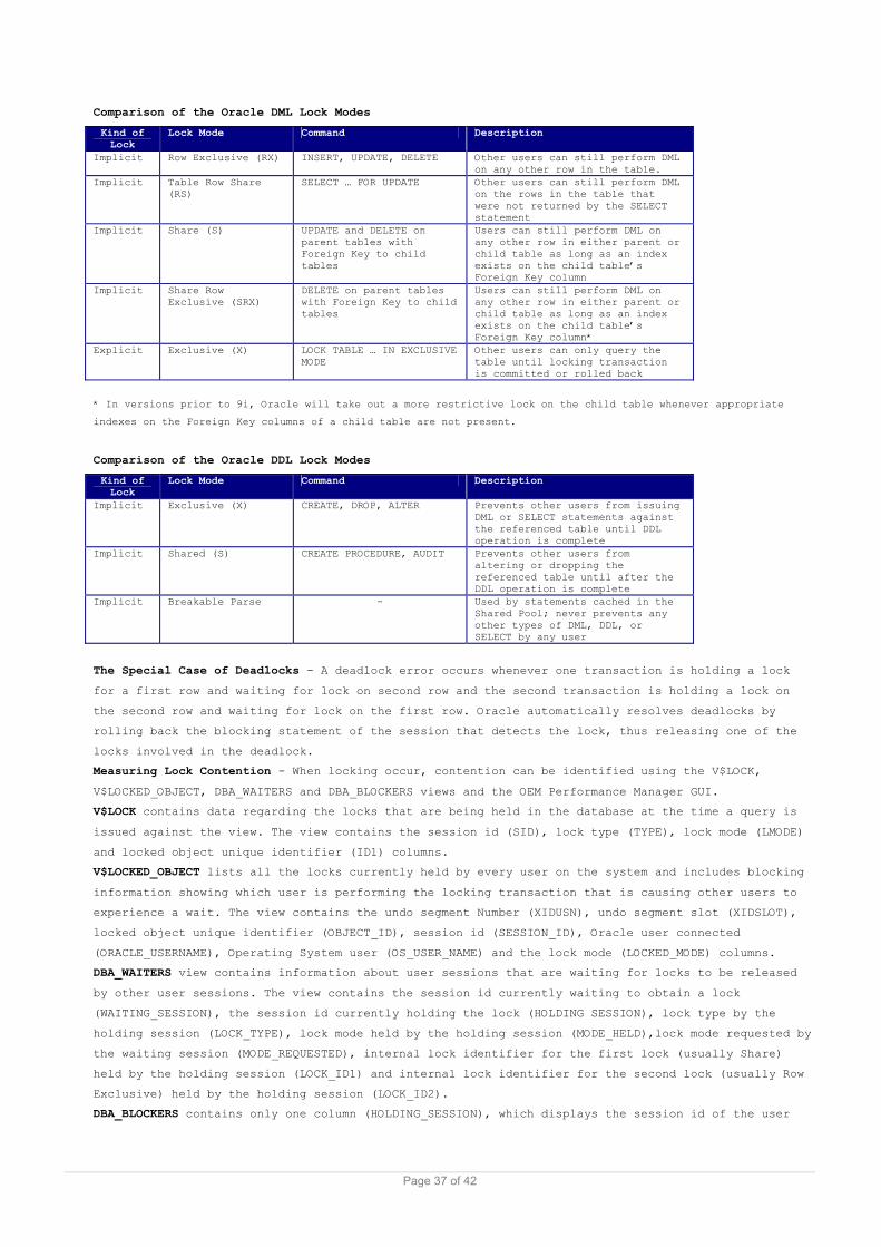
Comparison of the Oracle DML Lock Modes
Kind of Lock
Lock Mode Command Description
Implicit Row Exclusive (RX) INSERT, UPDATE, DELETE Other users can still perform DML on any other row in the table.
Implicit Table Row Share (RS)
SELECT … FOR UPDATE Other users can still perform DML on the rows in the table that were not returned by the SELECT statement
Implicit Share (S) UPDATE and DELETE on parent tables with Foreign Key to child tables
Users can still perform DML on any other row in either parent or child table as long as an index exists on the child table’s Foreign Key column
Implicit Share Row Exclusive (SRX)
DELETE on parent tables with Foreign Key to child tables
Users can still perform DML on any other row in either parent or child table as long as an index exists on the child table’s Foreign Key column*
Explicit Exclusive (X) LOCK TABLE … IN EXCLUSIVE MODE
Other users can only query the table until locking transaction is committed or rolled back
* In versions prior to 9i, Oracle will take out a more restrictive lock on the child table whenever appropriate
indexes on the Foreign Key columns of a child table are not present.
Comparison of the Oracle DDL Lock Modes
Kind of Lock
Lock Mode Command Description
Implicit Exclusive (X) CREATE, DROP, ALTER Prevents other users from issuing DML or SELECT statements against the referenced table until DDL operation is complete
Implicit Shared (S) CREATE PROCEDURE, AUDIT Prevents other users from altering or dropping the referenced table until after the DDL operation is complete
Implicit Breakable Parse - Used by statements cached in the Shared Pool; never prevents any other types of DML, DDL, or SELECT by any user
The Special Case of Deadlocks - A deadlock error occurs whenever one transaction is holding a lock
for a first row and waiting for lock on second row and the second transaction is holding a lock on
the second row and waiting for lock on the first row. Oracle automatically resolves deadlocks by
rolling back the blocking statement of the session that detects the lock, thus releasing one of the
locks involved in the deadlock.
Measuring Lock Contention - When locking occur, contention can be identified using the V$LOCK,
V$LOCKED_OBJECT, DBA_WAITERS and DBA_BLOCKERS views and the OEM Performance Manager GUI.
V$LOCK contains data regarding the locks that are being held in the database at the time a query is
issued against the view. The view contains the session id (SID), lock type (TYPE), lock mode (LMODE)
and locked object unique identifier (ID1) columns.
V$LOCKED_OBJECT lists all the locks currently held by every user on the system and includes blocking
information showing which user is performing the locking transaction that is causing other users to
experience a wait. The view contains the undo segment Number (XIDUSN), undo segment slot (XIDSLOT),
locked object unique identifier (OBJECT_ID), session id (SESSION_ID), Oracle user connected
(ORACLE_USERNAME), Operating System user (OS_USER_NAME) and the lock mode (LOCKED_MODE) columns.
DBA_WAITERS view contains information about user sessions that are waiting for locks to be released
by other user sessions. The view contains the session id currently waiting to obtain a lock
(WAITING_SESSION), the session id currently holding the lock (HOLDING SESSION), lock type by the
holding session (LOCK_TYPE), lock mode held by the holding session (MODE_HELD),lock mode requested by
the waiting session (MODE_REQUESTED), internal lock identifier for the first lock (usually Share)
held by the holding session (LOCK_ID1) and internal lock identifier for the second lock (usually Row
Exclusive) held by the holding session (LOCK_ID2).
DBA_BLOCKERS contains only one column (HOLDING_SESSION), which displays the session id of the user
Page 37 of 42
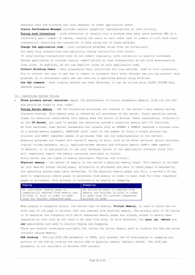
sessions that are blocking the lock requests of other application users.
Oracle Performance Manager includes several graphical representations of lock activity.
Tuning Lock Contention - Lock contention is usually only a problem when many users perform DML on a
relatively small number of tables, causing the users to wait other user to commit or roll back their
transaction. Resolving the contention is done using one of these methods:
Change the application code - Lock contention problems arise from two situations:
Too many long transactions and explicitly coding restrictive lock levels.
If long-running transactions that do not commit regularly, lock contention is greatly increased.
Design application to include logical commit points so that transactions do not hold unnecessarily
long locks. In addition, do not use explicit locks in your application code.
Contact Blocking Users - User suspending their activities for long periods, lead to lock contention.
Try to contact the user to get him to commit or rollback their work. Another way you can prevent this
problem, is to disconnect users who are idle for a specified period using Profiles.
Use SQL command – Once locking session has been detected, it can be killed using ALTER SYSTEM KILL
SESSION command.
10 - Operating System Tuning
• Three primary server resources impact the performance of Oracle databases: Memory, Disk I/O and CPU
and should be tuned in that order.
Tuning Server Memory - SGA and background processes are created in the server’s main memory during
instance startup. This memory area is shared by all processes on the server. Every operating system
loads its essential executables into memory when the server is booted. These executables, referred to
as the OS kernel, are used to manage the operating system’s essential memory and I/O functions.
On Unix machines, some Kernel Parameters are tunable such as SHMMAX & SHMMIN (maximum & minimum size,
of a shared memory segment), MAXFILES (soft limit on the number of files a single process can
utilize) and NPROC (maximum number of processes that can run simultaneously on the server).
Numerous programs are loaded into server's memory on boot, such as OS-level services (print services,
logical volume managers, etc…), Application/Web Servers and Software Agents (OEM's SNMP agents).
In general, it is bad practice to use your database server to run application software since this
will negatively impact the memory resources available to Oracle.
Every server has two types of memory available: Physical and Virtual.
Physical memory - the amount of memory in the server’s physical memory chips. This memory is divided
up into smaller pieces called pages. Allocation of processes and data to these pages is managed by
the operating system page table mechanism. If the physical memory pages are full, a server’s OS may
have to temporarily remove pages or processes from memory in order to make room for other requested
pages or processes. This process is referred to as paging or swapping.
Paging Swapping
An individual memory page is temporarily removed from memory and written to disk in order to make room for another requested page
An entire process is removed from memory and written to disk in order to make room for another requested process or page
When paging or swapping occurs, the second type of memory, Virtual Memory, is used to store the on-
disk copy of the page or process that was removed from physical memory. The primary goal of OS tuning
is to maximize the frequency with which requested memory pages are already cached in memory when
requested so that they do not need to be read from disk. On Unix machines, the ipcs, ps, vmstat and
sar executables are used to monitor Paging and Swapping.
There are several techniques available for tuning the server memory such as locking the SGA and using
Intimate Shared Memory:
SGA Locking – Setting LOCK_SGA parameter to TRUE, will prevent the OS from paging or swapping any
portion of the SGA by locking the entire SGA in physical memory (default FALSE). The LOCK_SGA
parameter is not available on Windows 2000 servers.
Page 38 of 42

Intimate Shared Memory - Database servers running the Sun Solaris operating system can also make use of
Intimate Shared Memory (ISM) to help tune OS paging and swapping activities. Enabling ISM allows
multiple OS processes to share access to the OS page tables that contain entries for shared memory
areas and, at the same time, locks the SGA into physical memory.
Tuning Server CPUs - The server’s CPU ultimately performs all the processing that occurs on a server.
If a server has multiple CPUs, then the processing tasks are shared among the available CPUs as
assigned by the server’s operating system.
Common Server Architectures:
Uniprocessor - Servers with a single CPU and memory area. I/O, bus, and disk resources are used
exclusively by this server.
Symmetric Multiprocessor (SMP) - Servers with two or more CPUs, but one memory area. I/O, bus, and
disk resources are used exclusively by this server.
Massively Parallel Processor (MPP) - Two or more servers connected together. Each server has its CPU,
memory area, I/O bus, disk drives, and a copy of the OS.
Non-Uniform Memory Access (NUMA) - Two or more SMP systems connected together. Each server has its
own CPU, but the memory areas for each server is shared as one large memory area across all servers.
A single copy of the OS is run across all servers.
Oracle is also a very CPU-aware product. If new CPUs are added to a database server, Oracle will
dynamically change the default settings for several CPU-related parameters.
CPU-related init.ora Parameters: CPU_COUNT - number of CPUs. PARALLEL_THREADS_PER_CPU - default
degree of parallelism when using parallel query/DML. FAST_START_PARALLEL_ROLLBACK - number of
parallel rollback processes (in instance recovery), valid values HIGH, LOW, FALSE, derived from the
number of CPUs. LOG_BUFFER - maximum size is 512K or 128K × the number of CPUs (whichever is higher).
PARALLEL_MAX_SERVERS - number of CPUs is one factor determining this parameter.
Additional CPUs most dramatically affect the performance of Oracle’s parallel execution features such
as Parallel Query, Parallel DML, Parallel ANALYZE, and Parallel Index Creation.
Parallel Query - allows a single query to spawn multiple query slaves, which work on a portion of the
query before the individual results are combined into a final result set. Parallel Query’s CPU usage
can be controlled through the use of the Resource Manager feature discussed later in this chapter
Parallel DML - Some DML activities can be performed in parallel using CREATE TABLE AS SELECT
statements and the /*+ PARALLEL */ SQL hint.
Parallel ANALYZE - Table and index statistics can be gathered in parallel using DBMS_STATS package.
Parallel Index Creation - Indexes created on large tables, can be created in parallel using the
PARALLEL keyword in the CREATE INDEX command. Using the PARALLEL keyword start multiple processes
that work together to create the index more quickly.
Tuning Processes and Threads - On Unix systems, each Oracle-related process runs as a separate and
distinct process. Each process consumes its own memory and CPU resources. On Windows systems, each
Oracle-related process runs as a separate thread within oracle.exe. A thread is an independent
sequence of instructions that executes within a single OS process. The process can contain multiple
threads.
Resource Manager - In Oracle versions prior to Oracle8i, resource consumption management was done
through the use of profiles. Oracle8i introduced a new feature, Resource Manager, which was designed
to improve the allocation and management of server resources needed by application users. Using the
Resource Manager, it is possible to create resource groups and assign them specific resource limits.
Resource Manager allows the DBA to limit the amount of CPU that an individual application user can
consume and the number of slave processes that an application user can spawn when performing Parallel
Query operations. Resource Manager can also be used to control resource allocations such as a user’s
maximum amount of undo segment usage and number of sessions against the database, thus ensuring
higher-priority resource groups to obtain sufficient CPU, memory, undo and session resources.
Page 39 of 42
The Oracle9i Resource Manager uses three components to achieve the goal of effective resource
management: resource consumer groups, resource plans, and resource plan directives:
Resource consumer group - A group of users who have similar needs for database resources. A user can
be a member of several resource groups, but only one group can be active at a time.
Resource plan - A collection of resource plan directives that are used to determine how resources are
allocated to users.
Resource plan directive - Specifies how many resources are allocated to each resource plan.
Resource Manager Resource - Resources that can be controlled through the use of Resource Manager
include these:
1. The amount of CPU allocated to each member of the resource consumer group
2. Parallel Queries degree of parallelism allowed for a member of the resource consumer group
3. The amount of undo segment space a member of a resource group is allowed to consume
4. The total number of active, concurrent sessions that a resource consumer group is allowed to have
5. The maximum expected time of a database action taken by a member of the resource consumer group
Managing CPU Resources - The CPU resources are allocated using the Emphasis method. The resources
associated with Parallel Query are assigned using the Absolute method. Both methods use a relative
scale, consisting of values from 1 (highest priority) to 8 (lowest priority) to determine what
priority should be assigned to a particular user’s request for resources.
Emphasis Method CPU Resources Management - The Emphasis method uses percentages to assign CPU
resources to each of the eight priority levels. The percentage assigned to a resource consumer group
at a given level determines the maximum amount of CPU that users can consume at that level. If excess
CPU resources remain after all users at that level have been serviced, then the remaining CPU
resources will be made available to users at the next level, and so on.
Absolute Method Parallel Query Resources Management - The Parallel Query (PQ) resource that is
controlled by Resource Manager is the degree of parallelism. Degree of parallelism refers to the
number of query slave processes that an individual session is allowed to start when processing its
query. The more query slaves started, the faster the query will be processed. However, this comes at
the expense of increased CPU utilization and disk I/O. Resource manager uses the Absolute method to
control Parallel Query resources. This means that the maximum degree of parallelism is a specific
(i.e., absolute) value.
Managing Undo Resources - Oracle9i introduces a new Plan Directive called the UNDO_PLAN, which
controls the amount of undo segment space a user is allowed to consume when executing a large DML
transaction. The limits placed on undo segment usage are implemented in the form of a quota for the
entire resource group. If the quota on undo segment space is exceeded, additional DML cannot be
performed by the user, or any other member of the user’s resource group, until another member of the
resource group releases undo resources.
Managing Workload Resources - The Active Session Pool, allows you to limit the number of active
concurrent sessions for a particular resource group. Once the members of the resource group reach the
number of allowed active concurrent sessions, any subsequent requests for active sessions will be
queued by Resource Manager instead of being processed immediately. Any queued sessions will be
executed after one or more of the existing sessions completes or becomes inactive. There is one queue
per resource consumer group. Queued sessions are allocated resources on a FIFO basis.
Configuring Resource Management:
Granting Resource Manager Privileges – Grant the ADMINISTER_RESOURCE_MANAGER privilege to users who
are going to manage Resource Groups, Plans, and Directives using DBMS_RESOURCE_MANAGER_PRIVS.
This package requires three arguments: GRANTEE_NAME, PRIVILEGE_NAME, and ADMIN_OPTION.
GRANTEE_NAME - name of the Oracle user being granted the privilege. PRIVILEGE_NAME - is the name of
the privilege being granted. ADMIN_OPTION - indicates whether the user receiving the privilege can
pass that privilege along to other users.
Creating the Resource Manager Objects - Setting up Resource Manager requires the following steps:
1. Creation of a pending area - Whenever a new resource consumer group, plan, or directive is
Page 40 of 42

created, it is temporarily stored in the pending area until it is validated and written to the
database. This gives the DBA the opportunity to confirm that the definitions of each consumer group,
plan, and directive are correct before implementing it. The pending area is created using the
DBMS_RESOURCE_MANAGER.CREATE_PENDING_AREA procedure.
2. Creation of one or more resource consumer groups - A resource consumer group is used to define a
group of application users who have similar resource requirements. By default, every application user
belongs to at least one RCG, which is called the DEFAULT_CONSUMER_GROUP. In addition, several other
RCGs are constructed at database creation: SYS_GROUP - has the highest priority for resource access.
SYS and SYSTEM are assigned to this RCG. LOW_GROUP – has the lowest priority for database resources.
Every user has access to this RCG. DEFAULT_CONSUMER_GROUP - Every user who is assigned to this RCG by
default. OTHER_GROUPS - The group to which all users belong when they are not members of the specific
resource plan that is currently active in the instance. Creating RCG is done through
DBMS_RESOURCE_MANAGER.CREATE_CONSUMER_GROUP procedure.
3. Creation of one or more resource plans - Resource plans are used to organize plan directives. A
group of plan directives can be assigned to a resource plan, which can in turn be assigned to one or
more resource groups. Only one resource plan can be active in the instance at a time. Creating
Resource Plans is done using the DBMS_RESOURCE_MANAGER.CREATE_PLAN procedure. Three default resource
plans, called SYSTEM_PLAN, INTERNAL_PLAN, and INTERNAL_QUIESCE, are created at database creation.
4. Creation of one or more resource plan directives - A plan directive is used to link a resource
consumer group to a resource plan. The plan directive is where the appropriate allocation of the
resources controlled by Resource Manager is specified (e.g., CPU, degree of parallelism). Plan
directives are created using the DBMS_RESOURCE_MANAGER.CREATE_PLAN_DIRECTIVE procedure.
5. Validation of the resource consumer groups, plans, and directives - Once a resource consumer group
has been defined and assigned a resource plan and directive, the entire package must be validated
before being written to the database. Verification is performed using the VALIDATE_PENDING_AREA
procedure of the DBMS_RESOURCE_MANAGER package.
6. Saving the resource consumer groups, plans, and directives to the database - Once the pending
resource consumer groups, plans, and directives have been validated, they must be committed to the
database before they can be assigned to database users. This commit is performed using the
DBMS_RESOURCE_MANAGER.SUBMIT_PENDING_AREA procedure.
Assigning Resources to Users - You can assign a resource consumer group to a database user by either
granting the RCG directly to an individual user, or by granting the RCG to a database role using the
DBMS_RESOURCE_MANAGER_PRIVS.GRANT_SWITCH_CONSUMER_GROUP procedure. Since a user can be a member of
several RCGs at one time, it is preferred to specify a default RCG that will be active for the user
when they initially connect to the database. (assigned using the SET_INITIAL_CONSUMER_GROUP
procedure in DBMS_RESOURCE_MANAGER package).
Once all the resource management groups, plans, and directives are in place and have been assigned to
users, the Resource Management feature must be enabled for the directives to take effect. If a user
is active for a specified period of time, Resource Manager can be configured to automatically switch
that user’s session to a secondary resource group. This feature is managed by specifying three
resource plan directive parameters:
SWITCH_TIME - used to specify the duration, in seconds (default 1,000,000), that a session must be
active before Resource Manager switches the session to the group specified by SWITCH_GROUP parameter
(default value NULL).
SWITCH_GROUP - If set to TRUE (default FALSE), Resource Manager will use the estimated execution time
to decide whether to assign the session to the SWITCH_GROUP before execution even begins, without
waiting for the execution time to exceed the value specified by SWITCH_TIME and SWITCH_ESTIMATE.
Setting Instance Resource Objectives - Any of the defined resource plans can be activated for the
instance. However, only one resource plan can be active at a time. The active resource plan for the
instance can be defined using the RESOURCE_MANAGER_PLAN parameter in init.ora, or by dynamically
issuing the ALTER SYSTEM SET RESOURCE_MANAGER_PLAN command. If this parameter is not set, then the
Page 41 of 42
Page 42 of 42
features of Resource Manager are disabled.
Oracle also gives you the ability to dynamically change the active RCG for an individual connected
user by using the DBMS_RESOURCE_MANAGER.SWITCH_CONSUMER_GROUP_FOR_USER procedure.
Changing active RCG is possible at session level also using the SWITCH_CONSUMER_GROUP_FOR_SESS
procedure in DBMS_RESOURCE package. This procedure accepts the SID and SERIAL# parameters as an
input.
Resource Manager Dynamic Performance Views - The three views that contain information related to
Resource Manager are:
V$SESSION - The RESOURCE_CONSUMER_GROUP column displays the current RCG for each session.
V$RSRC_CONSUMER_GROUP - contains details about the resource allocations that have been made to the
active resource consumer groups (CPU time, CPU waits etc…)
V$RSRC_PLAN – The NAME column displays the names of all the currently active resource plans.
Other Resource Manager related views are:
DBA_RSRC_CONSUMER_GROUPS - contains information on each resource consumer group in the database.
DBA_RSRC_CONSUMER_GROUPS_PRIVS - shows which users or roles in the database have been granted to each
resource consumer group.
DBA_RSRC_PLANS - shows all the resource plans that have been created in the database.
DBA_RSRC_PLAN_DIRECTIVES - displays the specific resource allocations that were assigned to each
resource plan.
DBA_RSRC_MANAGER_SYSTEM_PRIVS - contains information about which users have been granted the
DMINISTER_RESOURCE_MANAGER privilege.
DBA_USERS - The INITIAL_RSRC_CONSUMER_GROUP column indicates the resource consumer group that has
been assigned to a user as their default.
Resource Manager OEM Tools - The Instance section under the Database section of the OEM Console has
GUI tools that provide information on resource consumer groups and resource plans.
Top Related