


Languages
Pages
Legal

Page 1
ECGA 6470 Three Growth Models and Three Poverty Traps Spring 2016 Darryl McLeod Fordham University This handout reviews three basic growth models and several poverty traps: 1) The Harrod Domar model growth rate is γ = sA where s is the savings rate 1/A is the
ICOR or incremental capital output ratio, Y/K just as Y=AK .
2) The Solow or Neoclassical model where long run growth γ = n + λ where n and λ as ates
of population growth and λ is the exogenous rate of technical change.
3) The endogenous growth or "AK" model: γ = (1/θ)(A - ρ) where A is the fixed MPK,
1/θ is the intertemporal elasticity of substitution and ρ is intertemporal discount rate.
Introduction: Aggregate growth models make drastic simplifying assumptions to shed light on various
aspects of a very complex development process. Each new generation of growth models seeks to fix the
flaws of prior generations only to create new puzzles. Solow’s 1956 “Contribution to the theory of economic
growth” for example fixes the dynamic instability problem of the Harrod-Domar model but ends up saying
more about “steady state” income levels than determinates of long run growth: which in fact are assumed
hence these are “exogenous” growth models (models of LR incomes levels not growth). Growth models
became very sophisticated but did not say much about development and technical change at all.
Then in the mid-1980s macroeconomist Robert E. Lucas and his student Paul Romer created a new
generation of “endogenous” growth models.1 But as Charles Jones, 1995 points out, most R&D based
growth models imply an increasing growth rate. Fortunately, there is some common ground on the policy
implications of “alternative growth” models. In fact, the conditional convergence in the augmented Solow
model for example has policy implications similar to those of poverty trap models. Each break with the past
reveals yields new insights but considerable common ground remains. The endogenous growth literature of
the 1990s, promised a radical break with the past, but a series of “hybrid” models we review show all three
growth models share some common policy implications.
Generation 1: Harrod Domar (HD) growth model, γ = sA where s is the savings rate and the fixed A is
1 In his famous 1988 JME article Robert Lucas mentions a few growth rates, then comments,”I do not see how one can look at figures like these without seeing them as representing possibilities. Is there some action a government of India could take that would lead the Indian economy to grow like Indonesia's or Egypt's? If so, what, exactly? If not, what is it about the' nature of India' that makes it so? The consequences for human welfare involved in questions like these are simply staggering: Once one starts to think about them, it is hard to think about anything else”. (italics mine). Lucas is absolutely correct, hence this course. Amazingly India has started to grow rapidly as Indonesia did (why Egypt is fallen down a bit) lifting potential hundreds of millions more out of poverty over the next two decades. Following 1.5 billion heading into the 2015 MDGs development economists may soon be out of work… for good reason… (Lucas’s mechanics article trying to fix the Solow model has been cited well over 30,000 times, while Solow, 1956 has been cited 25k + (hence the need for three growth models of this handout instead of one…)

Page 2
average and marginal product of capital: The HD model starts with a few national accounting identities
and some strong assumptions, but still ends up with some interesting policy implications. Starting with the
national accounts identity Y = C + I (ignoring government and trade) Y, I and C are determined as in Hick’s
ISLM setup assuming a constant marginal propensity to consume or equivalently a fixed savings rate such
that I = sY and C = (1-s)Y. Investment or I is determined by exogenous “animal spirits” or by using a
simple accelerator model (increasing sales increases investment). Either way, once we know I (or I and G)
we know C and Y: Yd = (1/s)I where 1/s is the familiar “multiplier.” Supply or Ys is determined by the
simplest possible production function Y = AK where A is the fixed output to capital ratio, as clearly A=Y/K.
Or Ys = A(K+I) if new capital comes online instantly. Note that A is the average and the marginal product of
capital (APK = MPK). The famous incremental capital output ratio or ICOR is 1/A (β in Piketty’s 2nd
fundamental law of capitalism 𝜷𝜷 = 𝒔𝒔/𝒈𝒈). To complete the HD growth model we need a link between
investment I and the total capital stock K. Assuming no depreciation of capital ΔK = I = sY = sAK. Noting
that ΔY = A*ΔK and using the fact that ΔK = I = sY implies that the ΔY = sAY or using γ instead of g for
the growth rate , Y sA or sA
Yγ∆
= = .
Demand: (1) Yd = C + I where I is determined by an investment function and C = (1-s)Y so that Yd = (1/s)I = (1/s)ΔK
where we assume capital does not depreciate (Sachs et al.2004 & Jones Chapter 2 add d > 0).
Supply: (2) Ys = AK (note that the Robelo or AK model a direct descendant of the HD model, except that K in
the AK model includes human capital as well). Perhaps the most surprising implication of the HD model is that the
economy is dynamically unstable (see review question 1 below). A small in change in investment from its “warranted
rate” creates a growing excess of demand over supply, so the economy enters an inflationary spiral. A small decrease
in demand leads to a falling output and implicitly high unemployment and lost output (thought the HD model ignores
labor as input, as in Y = AK) In the mid-1950s Robert Solow looked outside and saw a fairly stable growing capitalist
economy with a tightening labor market and then wrote down the model that won him a noble prize (though it now
known as the Solow/Swan model). The modifications Solow made to the HD model seem obvious in retrospect, the
implications of assuming diminishing returns of capital to some exogenously determined input (scarce labor) was not
obvious. In fact growth model is in something of a misnomer: the Solow-Swan framework really gave us a model of
income levels, or steady states. “Endogenous growth” in the Solow model is always temporary or transitional: once
an economy reaches its steady state k*/y* only “exogenous” technical change or productivity growth remains.
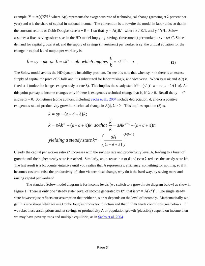
Generation 2: The Solow or Neoclassical model with a fixed savings rate implies a long run growth rate
of γ = n + λ where n and λ are the exogenous rates of population growth and technical change. The Solow-
Swan model adds a labor input that can be substituted for capital. With a Cobb-Douglas production function for
Page 3
example, Y = A(t)KαLβ where A(t) represents the exogenous rate of technological change (growing at λ percent per
year) and α is the share of capital in national income. The convention is to rewrite the model in labor units so that in
the constant returns or Cobb-Douglas case α + ß = 1 so that y = A(t)kα where k / K/L and y / Y/L. Solow
assumes a fixed savings share s, as in the HD model implying savings (investment) per worker is sy = sAkα. Since
demand for capital grows at nk and the supply of savings (investment) per worker is sy, the critical equation for the
change in capital k and output per worker y is,
1kk sy nk or k sk nk which implies sk nk
α α−= − = − = −
. (3)
The Solow model avoids the HD dynamic instability problem. To see this note that when sy > nk there is an excess
supply of capital the price of K falls and it is substituted for labor raising k, and vice versa. When sy = nk and A(t) is
fixed at 1 (unless it changes exogenously at rate λ). This implies the steady state k* = (s/n)μ where μ = 1/(1-α). At
this point per capita income changes only if there is exogenous technical change that is, if λ > 0. Recall that y = kα and set λ = 0. Sometimes (some authors, including Sachs et al., 2004 include depreciation, d, and/or a positive
exogenous rate of productivity growth or technical change in A(t), λ > 0. This implies equation (3) is,
1
1/(1 )
( )
( ) ;
( ) ( )
*n d
n d
n d n d
k sy k
kk sAk k sothat sAk nksAyielding a steady state k
α α
α
λ
λ
λ λ−
−
+ +
+ +
+ + + +
= −
= − = −
=
Clearly the capital per worker ratio k* increases with the savings rate and productivity level A, leading to a burst of
growth until the higher steady state is reached. Similarly, an increase in n or d and even λ reduces the steady-state k*.
The last result is a bit counter-intuitive until you realize that A represents x efficiency, something for nothing, so if it
becomes easier to raise the productivity of labor via technical change, why do it the hard way, by saving more and
raising capital per worker?
The standard Solow model diagram is for income levels (we switch to a growth rate diagram below) as show in
Figure 1. There is only one “steady state” level of income generated by k*, that is y* = A(k*)α . The single steady
state however just reflects our assumption that neither n, s or A depends on the level of income y. Mathematically we
get this nice shape when we use Cobb-Douglas production function and that fulfills Inada conditions (see below). If
we relax these assumptions and let savings or productivity A or population growth (plausibly) depend on income then
we may have poverty traps and multiple equilibria, as in Sachs et al. 2004.

Page 4
Generation 3: Endogenous growth or "AK" model with steady state growth rate:
γ = (1/θ)(A - ρ) Again start with Y = AK and Y = C + I so that per capita investment is I = Ak - c we
assume K includes both physical and human capital. The key assumption of endogenous growth models is
that even if labor and natural resources are in limited supply, growth can proceed without them using only
produced inputs: there are constant returns to produced inputs. An upgrade from the HD model is that
endogenous growth models solve for the Ramsey optimal savings rate assuming maximize a constant relative
risk aversion utility function along the lines of (1 )( 1)( )1
CU Cθ
θ
− −=
−
where 1/θ is the constant intertemporal elasticity of substitution (IES) and ρ is the discount rate (see the full
Barro Government and Growth handout for a formal derivation of this model-- since the MPK is constant at
A, it is important that IES be constant as well). In this new setup the savings rate depends on the parameters
σ and ρ which in turn depend on household preferences and under some interpretations, population growth
(since how one values the consumption in the future depends in part on how one values the consumption of
children). As 1/θ falls or ρ rises people to prefer consumption today over consumption tomorrow implying
they save less and growth falls. An important empirical implication of many (but not all) endogenous growth
models is that growth rates need show no convergence across countries and that the endogenous savings rate

Page 5
(or the parameter which affect time preference) is an important determinant of long term growth rate. Note
also that this model has a steady-state growth rate, but no steady income level (income grows forever). This
class of models is consistent with the roughly constant rate of per capita growth observed over long periods
in countries like the U.S., but this result relies on strong and key assumption: constant returns to produced
factors. Switching to Stone-Geary preferences: (see page 27 of Robelo, 1992) (1 )( ) 1( )
1C CU C
θ
θ
−− −=
− yields a low-income poverty trap, where C is subsistence consumption: as C falls
toward subsistence C the IES or 1/θ approaches zero and savings goes to zero creating a low savings poverty trap. Growth Models with and without Poverty traps: Perhaps the best way to gain some intuition about these models is by putting them into diagrams. Solow (1956) plots investment and the level of output y against the capital stock per worker, as in Figure 1. Under certain assumptions this model has unique stable solution also known as a steady state. Recall that the HD model has a solution, but it is dynamically unstable. Poverty trap models generally do not have a unique solution, rather they are likely to have two or more solutions or steady states a low-level equilibrium trap and the traditional higher income steady state. One way to assure a single solution (and to rule out most poverty traps) is to invoke the two Inada conditions. That is, when capital per worker gets very small (approaches zero) the marginal product of capital (MPK) approaches infinity, that is:
0lim '( )
kf k→
→∞ . Similarly, k becomes very large, the MPK approaches zero due to
diminishing returns that is, lim '( ) 0kf k→∞
→ . Taken assumptions give the Solow model diagram the shape
shown in Figure 1. The slope of the red lines reflects the MPK, the fact that it is very steep means these curves are very steep near the origin, always above the green population capital demand curve with slope n (the rate of population growth). However as k = K/L increases the MPK starts to fall towards zero, meaning at some point it must cross the green population line (slope n) from above, assuring the single steady state k*, y* as shown in Figure 5.

Page 6
Absolute Convergence: Return to (3) above we can rewrite the key dynamic equation as a growth rate by dividing
through by k, 1k sAk nk
α−= −
where if 0,kk=
then 0yy=
or at least the increment to y caused by an increase in k
goes to zero. Growth may continue due exogenous technical change, where AA
λ=
and assuming capital does not
depreciate at rate d or δ we obtain an exogenous growth rate of per capita y of γ determined by n and λ both of which
are determined outside the model for now (hence the term exogenous growth model). The standard Solow model has
one important testable implication: if two economies are heading toward the same steady state, for example k* in
Figure 2, then the low-income economy will tend to grow faster than the high income economy until both countries
reach their long run capital stock per worker k* and settle into the same long run growth rate per person λ (the
exogenous rate of technical change). Note that the HD model shows no such tendency, the economy with the highest
productivity savings rate combination sA will grow faster forever, there is not convergence. Prior to 2000, plotting
growth rates against initial per capital income (1960 or 1970) revealed no such pattern: poor economies did not grow

Page 7
faster than richer countries.
Conditional convergence: As Lucas (1988) points out, the original Solow model cannot explain the
variation in income across countries (there is not enough variation in capital per worker k) nor is it consistent
with the lack of absolute convergence discussed above. The empirical resurrection of the neoclassical
growth model rests on three modifications: one is to add human capital to obtain the “augmented Solow”
model explored by Mankiw, Romer and Weil (1992). Once human capital (typically years of education per
adult) is added to a growth regression, one obtains strong evidence for conditional convergence, and a large
proportion of variance in income levels across countries can be explained by human plus physical capital.2
Suppose kH in Figure 3 is the steady state associated with a high level of education, whereas kL reflects a
low level of human capital (using the approach of Jones (2002) Chapt 3 p 55) in this case
2 Sala-i-Martin (2004) argues evidence supporting conditional convergence demonstrates the validity of the augmented Solow model. Hybrid models also lead to convergence, as does the Sobelo model discussed below.

Page 8
kH Hk k whereh eAh
ψµ
= = =
, µ is average years of education and ψ reflects of the
productivity of human capital. In this case if we look at the data without controlling for human capital per
worker (differences in h) it will appear the rich country is growing faster than the poor country. Conditional
convergence says once we control for the education, we realize these countries are heading for different
steady states (the red vs. the blue k*). Conditional on education (for example) the poorer country is growing
faster than the rice country. Hence conditional convergence shifts our focus to why some countries have
higher steady state than others (e.g. higher savings rates, human capital investment, productivity, etc.).
Some growth models generate robust empirical results without a great deal of policy relevance. Conditional
convergence is a good example. Income levels converge to some extent, but to different steady states. If we define
steady states ex-post, in advertently, or pick a correlate as opposed to a cause of high steady state income, we may not
learn much of policy relevant. Strong absolute convergence has strong policy implications for government: just get out
of the way and let diminishing returns to labor work its magic. Relatively weak though robust conditional convergence
does not have strong result for policy, especially when there is some evidence higher incomes cause education, the
reverse of the MRW result. In a 2004 survey Sala-i-Martin argues “that the conditional convergence hypothesis is one
Page 9
of the strongest and most robust empirical regularities found in the data. Hence, by taking the theory seriously,
researchers arrived at the exact opposite empirical conclusion: the neoclassical model is not rejected by the data,
whereas the AK model is.” (Sala-i-Martin, 2004 p. 44). Though as he admits on the next page, some endogenous
growth models imply conditional convergence (including the hybrid Sobelo model described in Barro and Sala-i-
Martin, 2004). Other models with strong policy implications, poverty traps for example, are hard to find support for
empirically. To the extent that development involves more than growth, and countries seem to get stuck at the low
levels of development, the concept of multiple equilibria has strong appeal.
Three Poverty Traps Strong Inada conditions more or less guarantee a unique steady state in the Solow model. To explain
Africa’s lack of growth during the 1980s and 1990s, Sachs et al. (2004) argue governance indicators alone cannot
explain Africa’s underperformance. Solow model diagram above to illustrate three possible poverty traps
characterized by multiple equilibria and violations of one or more of the Inada conditions. Their Figure S-1 is
very similar to Figure 1 above, except that depreciation plus population growth d+ n drives the demand for
capital. And they use y = f(k) instead of (Cobb-Douglas case y=Akα we use above). The three poverty traps in
Sachs et al. 2004 make various parameters of the Solow model endogenous, specifically, A, n and s:
1. The minimum capital stock or productivity trap implies that as k→ 0, A(k) → 0 that is A(k) instead of
just A(t) as in the standard model (A(t) grows at exogenous rate λ above this minimum).
2. In a savings trap, Figure 3, the savings rate s(y) rises with income but s goes to zero as consumption
reaches some minimum level (e.g., C in the Stone-Geary utility function above, see also Robelo, 2002. P.27)
3. With demography trap, population growth is a function of income per worker, n(y), when income is too
low population growth is very rapid, as income rises, n falls.
In all three cases create a threshold beyond which steady state their KE (our k*) become unattainable
below some threshold value of k (Sachs et al. (2004) label this threshold level kT ) Once this threshold is
reached, the economy converges automatically to the higher steady state. This could be a local or a world steady
state, where OECD or U.S. per capita income levels represent the “frontier” of world technology, AW for example.
Below this threshold kT, the capital stock per worker falls steadily, negative growth pushing the economy into
poverty, hence the term “poverty trap.” Countries that are poor stay poor or become even poorer as k shrinks
(think of Malaria, Ebola, HIV or a series of natural disasters). Three Growth models questions for review:
1. Dynamic instability: The HD model is famously dynamically unstable in that a small deviation from its warranted” growth path leads to major booms and busts. To illustrate the “razor’s-edge” problem set s = .2, A = .333 and K = 120 then compute Yd = (1/s)*I and Ys = AK for I = 8. What is the growth rate g = ΔK/K = ΔY/Y where I = ΔK? This is the so-called warranted growth rate that makes Yd = Ys. Suppose investors become optimistic about the future and choose I = 10. What is the new Yd compared to Ys = AK or Ys = A(K+I)? What message does the resulting supply and demand imbalance send to firms? How would they respond? Try the same exercise with I = 5. How do these examples illustrate the “razor’s edge” problem? (see also Chaing p. 468).
2. The speed of convergence: When k is some distance away from its steady state value catch up growth
Page 10
can be quite dramatic. With s = .12, n = .03 and α = . 5 the steady state capital stock k* is 16. Write down the rate of change in k when the country has not yet reached its steady state k*? Now try k = 16, then k = 4, 8 or 12.
References: Lucas, R. (1988) “On the mechanics of economic development” Journal of Monetary Economics,22, 3-42 (over 33k citations on google scholar…) Mankiw, N.G. David Romer and David Weil (1992) “A contribution to the empirics of economic growth” QJE, v 107:1, 407-37. (16,800 + citations) Sachs, J., McArthur, J. W., Schmidt-Traub, G., Kruk, M., Bahadur, C., Faye, M., & McCord, G. (2004). Ending Africa's poverty trap. Brookings papers on economic activity, (1), 117-240 (863 citations) Piketty, Thomas (2014) About Capital in the 21st Century, Preview, AEA version Boston AEA Mankiw AEA preview Piketty presentation Rognlie Note Robelo, Sergio (1992) “Growth in Open Economies” Carnegie Series on Public Policy, 26, 5-46 (237 citations) Sala-i-Martin, Xavier 2004, Fifteen Years Of New Growth Economics: What Have We Learned?, Columbia University and Universitat Pompeu Fabra in Loayza, N. and R. Soto eds. Econ Growth Sources, trends and cycles, Vol 6, Central Bank of Chile) Solow, Robert M. (1956) “A contribution to the theory of economic growth” Quarterly Journal of Economics, LXX, 65-94 (cited 25k + times).

Page 11
1FIGURE S-1 (from Sachs et all, 2004, p. 124)

Page 12
FIGURE S-2 (from Sachs et all, 2004)

Page 13
2FIGURE S-3 (from Sachs et all, 2004, p. 126)

Page 14
3FIGURE S-4 (from Sachs et all, 2004 p. 129)

Page 15
This more general poverty trap diagram is discussed in the Banerjee and Duflo, 2011 Poor Economics (which is poor economics). It is more general in the sense that almost any stalled cumulative growth process (poverty trap) is consistent with this diagram. The above discussion of in this sense the Solow-Swan model is a specific example a may be more general phenomenon. The above poverty traps are considered supply side poverty traps, whereas the classic “Big Push” industrialization models posit poverty traps on the demand side.
Top Related