


Languages
Pages
Legal


Thermodynamical Modeling of a Car Cabin Physical Modeling Using the Simulink Toolbox, Simscape Master of Science Thesis in the Master Degree Program, Systems, Control and Mechatronics
LENA MÖLLER
LAUST SÖRENSEN
Department of Signal and Systems
Division of Mechatronics
CHALMERS UNIVERSITY OF TECHNOLOGY
Gothenburg, Sweden, 2011
Report No. EX005/2012
I
Abstract
The work carried out here is done to investigate if MathWorks Simulink toolbox Simscape, which is a
physical modeling toolbox, can be used to create a temperature model of a car cabin. Using Simscape
as the tool for modeling is an important factor because of its integration in the widely used MATLAB.
A thermodynamically model is created that will respond correctly with respect to air temperatures and
material temperatures in the cabin when exposed to different ambient temperatures, sun loads and
vehicle speeds that will change how fast the outer material of the car is cooled or heated. Also the air
entering the cabin through the ventilation nozzles is modeled so that the temperature on the inside can
be changed. The inflowing air is mixed with the air in the cabin and how this affects the temperature
change in the cabin is of great importance for the modeling.
The model does not contain any control loop so that a temperature can be kept constant in the cabin.
To verify the model, measurement data from a real car are used. The measurements used contain
ambient air temperature, inside temperature and the flow and temperature of the air at the nozzles.
From the verification of the model it is found that it is able to follow the measurement data when
exposed to the same conditions. This result means that it is possible to construct a temperature model
of a car cabin as intended. When more time is spent on understanding the physical properties, which
are working inside and outside the car cabin, the model can easily be changed so that it will work well
with other car models.

II
Preface
The base for this master thesis is to create a temperature model of a car cabin using the physical
modeling toolbox Simscape which is a part of Simulink that is a product from MathWorks. The main
objective is to investigate which physical properties that is at work within the cabin and how they can
be used in the Simscape language. This theoretical work together with experiments, carried out by
using Simscape, is arranged to a model which can simulate the temperature variations within the
cabin.
All work presented here is done at Volvo Car Corporation (VCC) at the group Climate Control
System within the electrical department where we wish to thank all that have been helpful with
answering question and contributing with good ideas to the project. Especially we wish to thank Jonas
Jange, our supervisor at VCC, for great support and input and also Ulf Gimbergsson for contributing
with input regarding modeling and simulation. In addition, we would which to thank Nina Andersson
and Daniel Wassmann for providing us with a lot of useful information regarding modeling and
measurement data. Finally we wish to thank Jonas Fredriksson, our supervisor at Chalmers, for
providing us with short and exact answers to our questions.
The authors have attended the master program Systems, Control and Mechatronics at Chalmers from
2009 – 2011. This program contains a wide range of courses where modeling and simulation, using
MATLAB/Simulink, is used for project work. Having this experience from using MATLAB/Simulink
and the knowledge of structuring a problem is an immense help for this work.
III
Contents
Abstract .................................................................................................................................................... I
Preface ................................................................................................................................................... II
Contents ................................................................................................................................................ III
Nomenclature ......................................................................................................................................... V
1. Introduction ................................................................................................................................ - 1 -
1.1. Objective ............................................................................................................................ - 1 -
1.2. Limitations ......................................................................................................................... - 1 -
1.3. Method ............................................................................................................................... - 1 -
1.4. Outline................................................................................................................................ - 2 -
2. Theory ........................................................................................................................................ - 3 -
2.1. Conduction ......................................................................................................................... - 3 -
2.1.1. Steady State Conduction ............................................................................................ - 3 -
2.1.2. Transient Heat Conduction and Multi Dimensions .................................................... - 5 -
2.2. Convection ......................................................................................................................... - 5 -
2.2.1. Velocity Boundary Layer ........................................................................................... - 6 -
2.2.2. Thermal Boundary Layer ........................................................................................... - 7 -
2.2.3. Turbulent and Laminar Flow ..................................................................................... - 7 -
2.2.4. Convection Heat Transfer Coefficient ....................................................................... - 8 -
2.2.5. Natural and Forced Convection ................................................................................. - 8 -
2.2.6. Dimensionless Numbers ............................................................................................ - 9 -
2.2.7. Combined Natural and Forced Convection .............................................................. - 10 -
2.3. Radiation .......................................................................................................................... - 11 -
2.3.1. Black Body ............................................................................................................... - 12 -
2.3.2. Gray Body ................................................................................................................ - 12 -
3. Modeling in Simscape .............................................................................................................. - 14 -
3.1. Physical Modeling – Simscape vs. Dymola ..................................................................... - 14 -
3.2. Differences between Simulink and Simscape Modeling ................................................. - 14 -
3.2.1. Heat Transfer in Simscape ....................................................................................... - 15 -
3.2.2. Code ......................................................................................................................... - 16 -
3.2.3. Through and Across Variables ................................................................................. - 16 -
3.2.4. Physical Domains ..................................................................................................... - 16 -
3.2.5. Components ............................................................................................................. - 17 -
3.2.6. Example of a Simple Simscape Model .................................................................... - 18 -
3.3. Creating a Custom Component in Simscape .................................................................... - 20 -
3.4. Air Masses ....................................................................................................................... - 23 -
3.5. Materials in Simscape and How They are Connected to Air Masses .............................. - 26 -
IV
3.6. Comparison of Multi Layer Material and a Single Layer Material Model ...................... - 28 -
3.7. Solvers.............................................................................................................................. - 34 -
3.7.1. Choosing a Solver for Simscape .............................................................................. - 35 -
3.7.2. Solver Choice for a Simscape Model and Tests ....................................................... - 35 -
4. The Car Compartment Temperature Model in Simscape ........................................................ - 38 -
4.1. Measurement Data ........................................................................................................... - 38 -
4.2. Simplifications and Assumptions ..................................................................................... - 38 -
4.3. What the Model Includes ................................................................................................. - 39 -
4.4. Constructing the Model .................................................................................................... - 39 -
4.5. Adjusting Parameters to fit Measurement Data ............................................................... - 43 -
5. Advantages and Drawbacks with Physical Modeling in Simscape .......................................... - 47 -
6. Results ...................................................................................................................................... - 48 -
7. Conclusion ............................................................................................................................... - 54 -
7.1. Results and Discussion .................................................................................................... - 54 -
7.2. Future Work ..................................................................................................................... - 55 -
8. References ................................................................................................................................ - 56 -
V
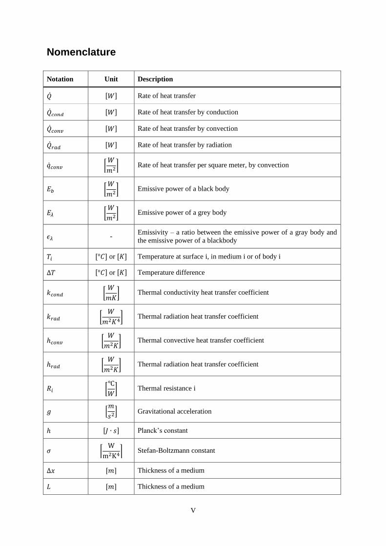
Nomenclature
Notation Unit Description
[ ] Rate of heat transfer
[ ] Rate of heat transfer by conduction
[ ] Rate of heat transfer by convection
[ ] Rate of heat transfer by radiation
[
] Rate of heat transfer per square meter, by convection
[
] Emissive power of a black body
[
] Emissive power of a grey body
- Emissivity – a ratio between the emissive power of a gray body and
the emissive power of a blackbody
[ ] or [ ] Temperature at surface , in medium or of body
[ ] or [ ] Temperature difference
[
] Thermal conductivity heat transfer coefficient
[
] Thermal radiation heat transfer coefficient
[
] Thermal convective heat transfer coefficient
[
] Thermal radiation heat transfer coefficient
[
] Thermal resistance
[
] Gravitational acceleration
[ ] Planck’s constant
[
] Stefan-Boltzmann constant
[ ] Thickness of a medium
[ ] Thickness of a medium

VI
[ ] Characteristic length
[ ] Wave length
[ ] Area
[
] Density
[
] Coefficient of volume expansion
[
] Specific heat
[
] Velocity of liquid or gas in motion
[
] Kinematic viscosity
[
] Dynamic viscosity of a liquid or gas
[ ] Wave propagation speed
- Nusselt Number represents how much the heat transfer is increased
due to convection
- Reynolds Number – to determine if the flow is turbulent, laminar or
somewhere in between, connected to forced convection
- Grashof Number – equivalent to Reynolds number, but connected to
natural convection

- 1 -
1. Introduction
When developing the climate control function either for better performance or to be used in a future
car model, the new functionality has to be verified. It is expensive to perform all verifications and
tests in real vehicles. It is not only necessary to have a car with test and measurement equipment, also
some kind of climate chambers or wind tunnels are essential where it is possible to control the
surrounding climate with ambient temperature and wind speed, which are parameters that
significantly affect the temperature inside the car cabin. Also depending on how early it is in the
product development process of a future car model there is not always a physical car available to
perform tests and verifications in.
To overcome the need of a real vehicle and test environment there is a desire to construct a model
representing how the temperature develops within the car cabin, using mass flow rate and temperature
from the air inlets as inputs. In a mathematical model the user need to set up all the equations of the
system in order to simulate it, but in a physical model components, e.g. pumps and pipes, are put
together and the modeling tool automatically analyze and solve the equations that constitutes the
system. Compared to a mathematical model, a physical model is more intuitive and easier to
understand. In a physical model it is also easier to see what is missing and to add and test new or
different conditions, e.g. the impact of radiation, both from the sun between materials.
The idea is to have a plant model representing the cars behavior regarding temperature development
in the compartment and use this model to test the control algorithm against.
1.1. Objective
The goal is to investigate if it is possible to represent the temperature distribution in a car cabin with a
model based on physical insight.
1.2. Limitations
It is preferred to simplify the model as much as possible in order to keep calculation time on a
reasonable level. Especially the materials can be simplified, e.g. a car door is very complex with
several materials geometries. Therefore it is also difficult to calculate the exact heat transfer through
the door. For these reasons the emphasis is not on finding the exact material data, to construct
complex shapes and calculating heat transfer through them, but rather on estimating the total heat
transfer from the inside to the outside of the car cabin and fitting the model to measurement data.
1.3. Method
The work method can be described by the following steps:
1. At first theories and fundamentals of thermodynamics are studied, especially the effect of
conduction, convection and radiation
2. The second step is to learn how Simscape works, both the basics of physical modeling in
Simscape and the parts related to a thermal and pneumatic models
3. Then a model with connected air masses, materials, orifices and a mass flow rate source is
constructed. This model just represents any closed room, without being related to a car.
Though it certainly include most parts needed to construct the temperature model of a car
compartment
4. Finally the temperature model of a car cabin is constructed, tuned and verified against
measurement data
- 2 -
1.4. Outline
The report mainly consists of three parts. First an overview of the most important theory within
thermodynamics, like the effect of conduction, convection and radiation, is described in chapter 2. In
chapter 3 modeling in Simscape is described, both from a general view and the specific parts needed
for a temperature model and in chapter 4 it is explained how the temperature model is constructed and
validated. This is followed by how the model parameters are tuned. By the end of the report there are
results, advantages and drawbacks with physical modeling and conclusions.

- 3 -
2. Theory
2.1. Conduction
According to [1] heat transfer through thermal conduction can occur in gases, liquids and solids. In
gases and liquids the heat transfer happens due to collision and diffusion of the molecules during their
random motion. In solids the heat transfer is a combination of the vibrations of the molecules and
energy transport of free electrons. How fast the heat is conducted through a medium depends on the
shape of the medium, the thickness and the material of the medium and the temperature difference
across the medium. The thermal conductivity is expressed as , where W is Watts, m is length
in meter and K temperature in Kelvin. In table 1 a few values from [2] for gasses, liquids and solids
are listed. It is clear that metals have the best heat transfer rate while the others have considerable less.
Table 1: Values for thermal conductivity found in [1]
Material W/m*K
Copper 385
Iron 73
Glass 0.78
PVC 0.09
Water 0.556
Air 0.024
2.1.1. Steady State Conduction
According to [1] heat transfer is in the most general case in three dimensions through a medium. Also
according to [1] does this mean that the temperature varies along all three primary directions within
the medium during the heat transfer process. This heat transfer is considered to be transient since the
temperature in the medium and the surroundings is varying and thus the heat flow will vary. Steady
state conditions will only exist when the temperatures are constant. Using figure 1 as an example the
steady state conditions will exist when the temperature on both sides of the wall are kept constant for
a long time so that the temperature within the wall is no longer changing. To make the analysis of the
heat transfer simpler it can in [1] be found that most problems are analyzed under some presumed
steady state conditions. Further simplification done here is only to assume heat transfer in one
dimension which means that the temperature varies only in one direction. Heat transfer in the other
directions is neglected or considered to be zero. This simplification can be done for larger surfaces
where the thickness is small compared to the surface areas that are used for the analysis.
Figure 1 shows a wall with thickness L and the temperatures and on either side. The sloped line
between the temperatures indicates the temperature change through the wall at steady state conditions.
The heat transfer is then calculated as
[ ]
(1)
where [ ] [ ] [ ] [ ] [ ]

- 4 -
Equation (1) can be expressed as a differential equation when .
[ ]
(2)
This differential form is also called the Fourier’s law of heat conduction after the French
mathematical physicist Joseph Fourier according to [2].
As mentioned before the heat transfer rate depends on the shape and material or the thermal property
of the medium. From this we get the thermal conductivity which like in electrical circuits is the
inverse of resistance. This resistance is called the thermal resistance, figure 2, or the conduction
resistance. By integrating equation (2) and by replacing the distance x with the thickness of the wall L
the heat transfer rate for the wall can be expressed like
[ ]
(3)
Equation (3) can be compared to the equation for electrical current where the current I is the heat
transfer rate and the voltage V is the temperature difference across the wall, . Then
becomes the conductivity of the system, 1/R, thus the thermal resistance is dependent on the area A,
the thickness L and k the thermal conductivity.
[ ]
(4)
On either side of the wall the heat has to flow into or out of the wall, depending on the temperature on
the sides. This heat transfer is due to a combination of convection and radiation. These forms of heat
transfer will be described later on in this chapter. In [1] it is described that by adding radiation and
convection to either side of the wall the total heat transfer coefficient for the wall can be found. Since
the convection and radiation is a simultaneous process they are placed in parallel. To avoid
complications when calculating the thermal resistance for the wall and its surroundings the radiation
and convection are combined. This is done by assuming that the surrounding temperature is equal
to the temperature far from the surface. Using this assumption the heat transfer coefficient for
radiation and convection can be combined and then only this combined coefficient is used in the
convective heat transfer resistance. Equation (5) and (6) are the thermal resistances for convection and
radiation and (7) the combined heat transfer coefficient. In figure 3 the temperature variation from the
surface of the wall to a point far from the wall is shown for both sides where TA is the high
temperature and TB is the low temperature. The thermal resistance for the wall and the convection
Figure 2: The thermal resistance of a wall described as an electrical circuit.
Figure 1: Steady state temperature distribution in a plane wall from [1].
L (x)
T1
T2
Wall
- 5 -
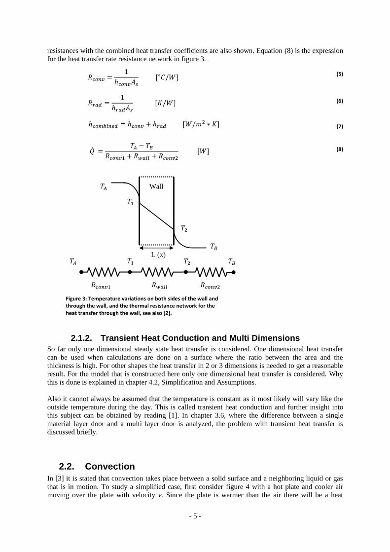
resistances with the combined heat transfer coefficients are also shown. Equation (8) is the expression
for the heat transfer rate resistance network in figure 3.
[ ]
(5)
[ ]
(6)
[ ]
(7)
[ ]
(8)
2.1.2. Transient Heat Conduction and Multi Dimensions
So far only one dimensional steady state heat transfer is considered. One dimensional heat transfer
can be used when calculations are done on a surface where the ratio between the area and the
thickness is high. For other shapes the heat transfer in 2 or 3 dimensions is needed to get a reasonable
result. For the model that is constructed here only one dimensional heat transfer is considered. Why
this is done is explained in chapter 4.2, Simplification and Assumptions.
Also it cannot always be assumed that the temperature is constant as it most likely will vary like the
outside temperature during the day. This is called transient heat conduction and further insight into
this subject can be obtained by reading [1]. In chapter 3.6, where the difference between a single
material layer door and a multi layer door is analyzed, the problem with transient heat transfer is
discussed briefly.
2.2. Convection
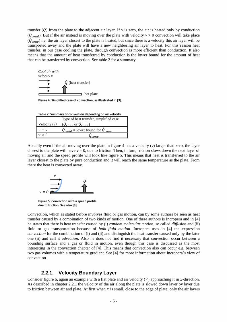
In [3] it is stated that convection takes place between a solid surface and a neighboring liquid or gas
that is in motion. To study a simplified case, first consider figure 4 with a hot plate and cooler air
moving over the plate with velocity v. Since the plate is warmer than the air there will be a heat
L (x)
Wall
Figure 3: Temperature variations on both sides of the wall and through the wall, and the thermal resistance network for the heat transfer through the wall, see also [2].
- 6 -
transfer ( ) from the plate to the adjacent air layer. If v is zero, the air is heated only by conduction
( ). But if the air instead is moving over the plate with velocity v > 0 convection will take place
( ) i.e. the air layer closest to the plate is heated, but since there is a velocity this air layer will be
transported away and the plate will have a new neighboring air layer to heat. For this reason heat
transfer, in our case cooling the plate, through convection is more efficient than conduction. It also
means that the amount of heat transferred by conduction is the lower bound for the amount of heat
that can be transferred by convection. See table 2 for a summary.
Figure 4: Simplified case of convection, as illustrated in [3].
Table 2: Summary of convection depending on air velocity
Velocity (v)
Type of heat transfer, simplified case
( or )
= lower bound for
Actually even if the air moving over the plate in figure 4 has a velocity (v) larger than zero, the layer
closest to the plate will have v = 0, due to friction. Then, in turn, friction slows down the next layer of
moving air and the speed profile will look like figure 5. This means that heat is transferred to the air
layer closest to the plate by pure conduction and it will reach the same temperature as the plate. From
there the heat is convected away.
Convection, which as stated before involves fluid or gas motion, can by some authors be seen as heat
transfer caused by a combination of two kinds of motion. One of these authors is Incropera and in [4]
he states that there is heat transfer caused by (i) random molecular motion, so called diffusion and (ii)
fluid or gas transportation because of bulk fluid motion. Incropera uses in [4] the expression
convection for the combination of (i) and (ii) and distinguish the heat transfer caused only by the later
one (ii) and call it advection. Also he does not find it necessary that convection occur between a
bounding surface and a gas or fluid in motion, even though this case is discussed as the most
interesting in the convection chapter of [4]. This means that convection also can occur e.g. between
two gas volumes with a temperature gradient. See [4] for more information about Incropera’s view of
convection.
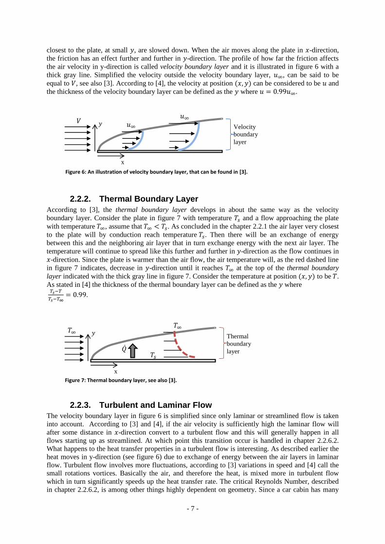
2.2.1. Velocity Boundary Layer
Consider figure 6, again an example with a flat plate and air velocity ( ) approaching it in -direction.
As described in chapter 2.2.1 the velocity of the air along the plate is slowed down layer by layer due
to friction between air and plate. At first when is small, close to the edge of plate, only the air layers
v
v = 0
hot plate
Cool air with
velocity v
(heat transfer)
Figure 5: Convection with a speed profile due to friction. See also [3].
- 7 -
closest to the plate, at small , are slowed down. When the air moves along the plate in -direction,
the friction has an effect further and further in -direction. The profile of how far the friction affects
the air velocity in y-direction is called velocity boundary layer and it is illustrated in figure 6 with a
thick gray line. Simplified the velocity outside the velocity boundary layer, , can be said to be
equal to , see also [3]. According to [4], the velocity at position can be considered to be and
the thickness of the velocity boundary layer can be defined as the where .
2.2.2. Thermal Boundary Layer
According to [3], the thermal boundary layer develops in about the same way as the velocity
boundary layer. Consider the plate in figure 7 with temperature and a flow approaching the plate
with temperature , assume that . As concluded in the chapter 2.2.1 the air layer very closest
to the plate will by conduction reach temperature . Then there will be an exchange of energy
between this and the neighboring air layer that in turn exchange energy with the next air layer. The
temperature will continue to spread like this further and further in -direction as the flow continues in
-direction. Since the plate is warmer than the air flow, the air temperature will, as the red dashed line
in figure 7 indicates, decrease in -direction until it reaches at the top of the thermal boundary
layer indicated with the thick gray line in figure 7. Consider the temperature at position to be .
As stated in [4] the thickness of the thermal boundary layer can be defined as the where
.
Figure 7: Thermal boundary layer, see also [3].
2.2.3. Turbulent and Laminar Flow
The velocity boundary layer in figure 6 is simplified since only laminar or streamlined flow is taken
into account. According to [3] and [4], if the air velocity is sufficiently high the laminar flow will
after some distance in -direction convert to a turbulent flow and this will generally happen in all
flows starting up as streamlined. At which point this transition occur is handled in chapter 2.2.6.2.
What happens to the heat transfer properties in a turbulent flow is interesting. As described earlier the
heat moves in y-direction (see figure 6) due to exchange of energy between the air layers in laminar
flow. Turbulent flow involves more fluctuations, according to [3] variations in speed and [4] call the
small rotations vortices. Basically the air, and therefore the heat, is mixed more in turbulent flow
which in turn significantly speeds up the heat transfer rate. The critical Reynolds Number, described
in chapter 2.2.6.2, is among other things highly dependent on geometry. Since a car cabin has many
x
Thermal
boundary
layer
x
Velocity
boundary
layer
Figure 6: An illustration of velocity boundary layer, that can be found in [3].
- 8 -
odd geometries and flow from several directions it is hard or even impossible to estimate if there is
laminar or turbulent flow inside the compartment. Therefore the heat transfer coefficient in this work
is simplified to be linear dependent on the mass flow rate. For more details about turbulent and
laminar flow and how it affects the heat transfer, it is recommended to read the chapters concerning
this in [3] or [4].
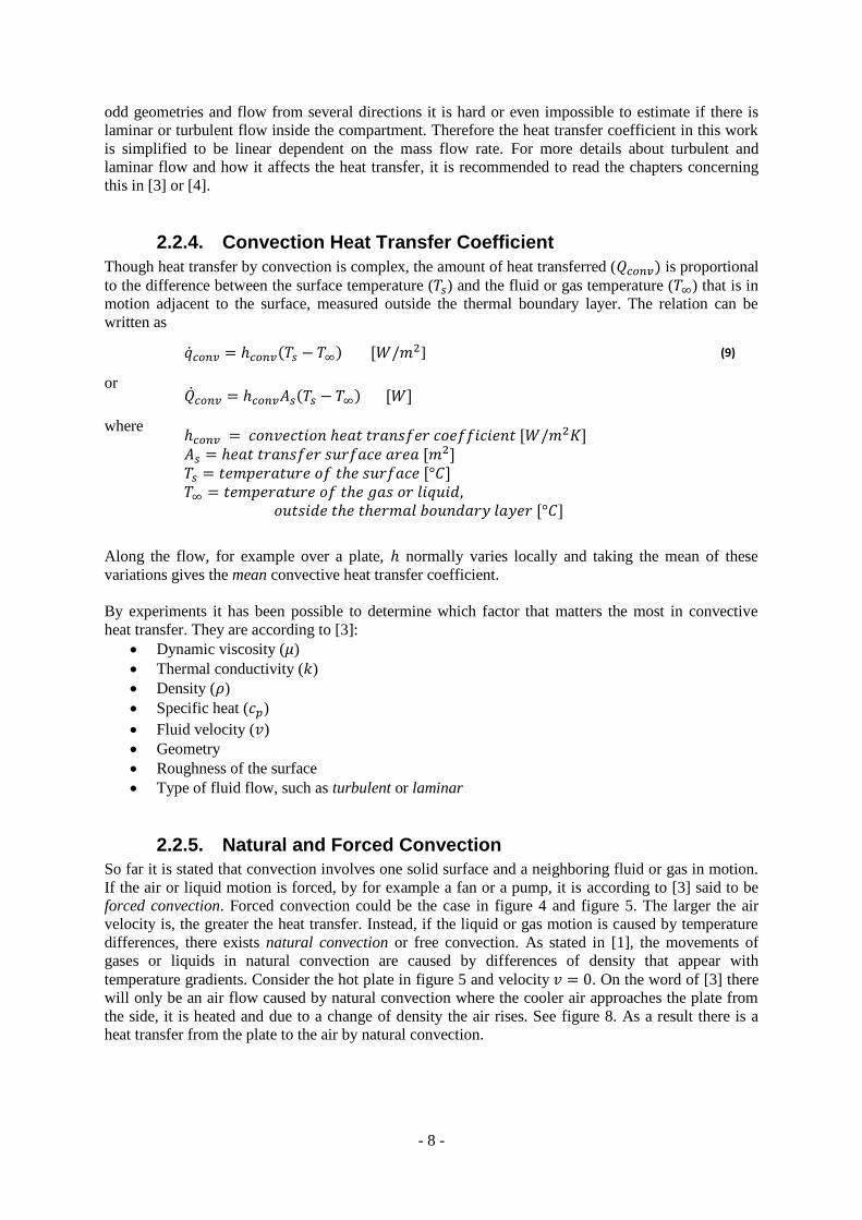
2.2.4. Convection Heat Transfer Coefficient
Though heat transfer by convection is complex, the amount of heat transferred ( is proportional
to the difference between the surface temperature ( ) and the fluid or gas temperature ( ) that is in
motion adjacent to the surface, measured outside the thermal boundary layer. The relation can be
written as
[ ] (9)
or [ ]
where [ ] [ ] [ ]
[ ]
Along the flow, for example over a plate, normally varies locally and taking the mean of these
variations gives the mean convective heat transfer coefficient.
By experiments it has been possible to determine which factor that matters the most in convective
heat transfer. They are according to [3]:
Dynamic viscosity ( )
Thermal conductivity ( )
Density ( )
Specific heat ( )
Fluid velocity ( )
Geometry
Roughness of the surface
Type of fluid flow, such as turbulent or laminar
2.2.5. Natural and Forced Convection
So far it is stated that convection involves one solid surface and a neighboring fluid or gas in motion.
If the air or liquid motion is forced, by for example a fan or a pump, it is according to [3] said to be
forced convection. Forced convection could be the case in figure 4 and figure 5. The larger the air
velocity is, the greater the heat transfer. Instead, if the liquid or gas motion is caused by temperature
differences, there exists natural convection or free convection. As stated in [1], the movements of
gases or liquids in natural convection are caused by differences of density that appear with
temperature gradients. Consider the hot plate in figure 5 and velocity . On the word of [3] there
will only be an air flow caused by natural convection where the cooler air approaches the plate from
the side, it is heated and due to a change of density the air rises. See figure 8. As a result there is a
heat transfer from the plate to the air by natural convection.

- 9 -
Figure 8: Natural convection, as illustrated in [3].
2.2.6. Dimensionless Numbers
In this chapter follows some dimensionless numbers that are important when discussing convection.
2.2.6.1. Nusselt Number
The Nusselt Number ( ) is a dimensionless number that represents how much the heat transfer is
increased due to convection, compared to if only conduction exists. Çengel [3] states that
(10)
where [ ] [ ] [ ] [ ]
2.2.6.2. Reynolds Number
Reynolds number is connected to forced convective flow and it is a measurement to determine if the
flow is turbulent, laminar or somewhere in between, in the so called transition region. At which point
the laminar flow becomes turbulent is in reality dependent on several variables, e.g. roughness,
temperature and geometry of the surface as well as velocity and type of fluid. But according to [3]
experiments performed by Osborn Reynolds in late 19th century showed that the type of flow mainly
depends on the quote between inertia forces and viscous forces resulting in the Reynolds number. The
Reynolds number can be calculated as
(11)
where
[ ] [ ]
[ ]
[ ] [ ]
If the inertia forces are greater relative to the viscous forces there is a turbulent flow and a large
Reynolds number. If instead, the viscous forces are large compared to the inertia forces there is
laminar flow and a small Reynolds number. Viscosity is greatly dependent on temperature mainly for
two reasons. First the inertia forces are proportional to the density which changes with temperature.
Secondly, the viscosity is a measurement of resistance to flow, which also changes with temperature.
When temperature increases, the viscosity of gases also increases and the viscosity of liquids
decreases. The characteristic length ( ) depends on the solid geometry and its size. For standard
hot plate
Heated air
is rising
- 10 -
shapes can be found in tables. The critical Reynolds number identify when the laminar flow
converts to turbulent flow, see also [3].
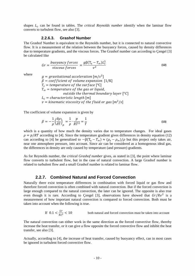
2.2.6.3. Grashof Number
The Grashof Number is equivalent to the Reynolds number, but it is connected to natural convective
flow. It is a measurement of the relation between the buoyancy forces, caused by density differences
due to temperature gradients, and the viscous forces. The Grashof number can according to Çengel [3]
be calculated like
(12)
where [ ] [ ] [ ] [ ] [ ] [ ]
The coefficient of volume expansion is given by
(
)
(13)
which is a quantity of how much the density varies due to temperature changes. For ideal gases
according to [4]. Since the temperature gradient gives differences in density equation (12)
can according to [4] be generalized to but this project only takes air,
near one atmosphere pressure, into account. Since air can be considered as a homogenous ideal gas,
the differences in density are only caused by temperature (and pressure) gradients.
As for Reynolds number, the critical Grashof number gives, as stated in [3], the point where laminar
flow converts to turbulent flow, but in the case of natural convection. A large Grashof number is
related to turbulent flow and a small Grashof number is related to laminar flow.
2.2.7. Combined Natural and Forced Convection
Naturally there exist temperature differences in combination with forced liquid or gas flow and
therefore forced convection is often combined with natural convection. But if the forced convection is
large enough compared to the natural convection, the later can be ignored. The opposite is also true
even though it is rare. According to Çengel [3], observations have showed that is a
measurement of how important natural convection is compared to forced convection. Both must be
taken into account when the following is true.
If
both natural and forced convection must be taken into account
The natural convection can either work in the same direction as the forced convective flow, thereby
increase the heat transfer, or it can give a flow opposite the forced convective flow and inhibit the heat
transfer, see also [3].
Actually, according to [4], the increase of heat transfer, caused by buoyancy effect, can in most cases
be ignored in turbulent forced convective flow.
- 11 -
2.3. Radiation
Unlike conduction and convection, where heat is transferred through a medium or from the surface of
it into the surrounding air, radiation can transfer heat from one object to another through vacuum.
This type of heat transfer occurs in solids, liquids and gases. The energy transfer by radiation is
through electromagnetic waves which originate from the change in the electronic configuration in the
atoms or molecules. The electromagnetic waves vary in wave length from 10-10
m for cosmic rays to
1010
m for electric power waves. The wave length determines how much energy that is transmitted
which can be expressed like
[ ] (14)
where [ ] [ ] [ ] [ ]
From equation (14) it can be seen that a short wave length will give a higher energy level than a long
wave length would.
In [5] it is stated that substance, that has a temperature that is above absolute zero, will emit thermal
radiation. This thermal radiation has a wave length between 0.1μm and 100μm. In this region the
ultraviolet light is the most energetic because of the shorter wave length. The visible light with its
wave length from 0.4μm to 0.76μm follows the ultraviolet light. The last waves that are in the thermal
region are the infrared waves which cover the wave length from about 1um to 100μm. As well as all
things emit thermal radiation they also absorb radiation.
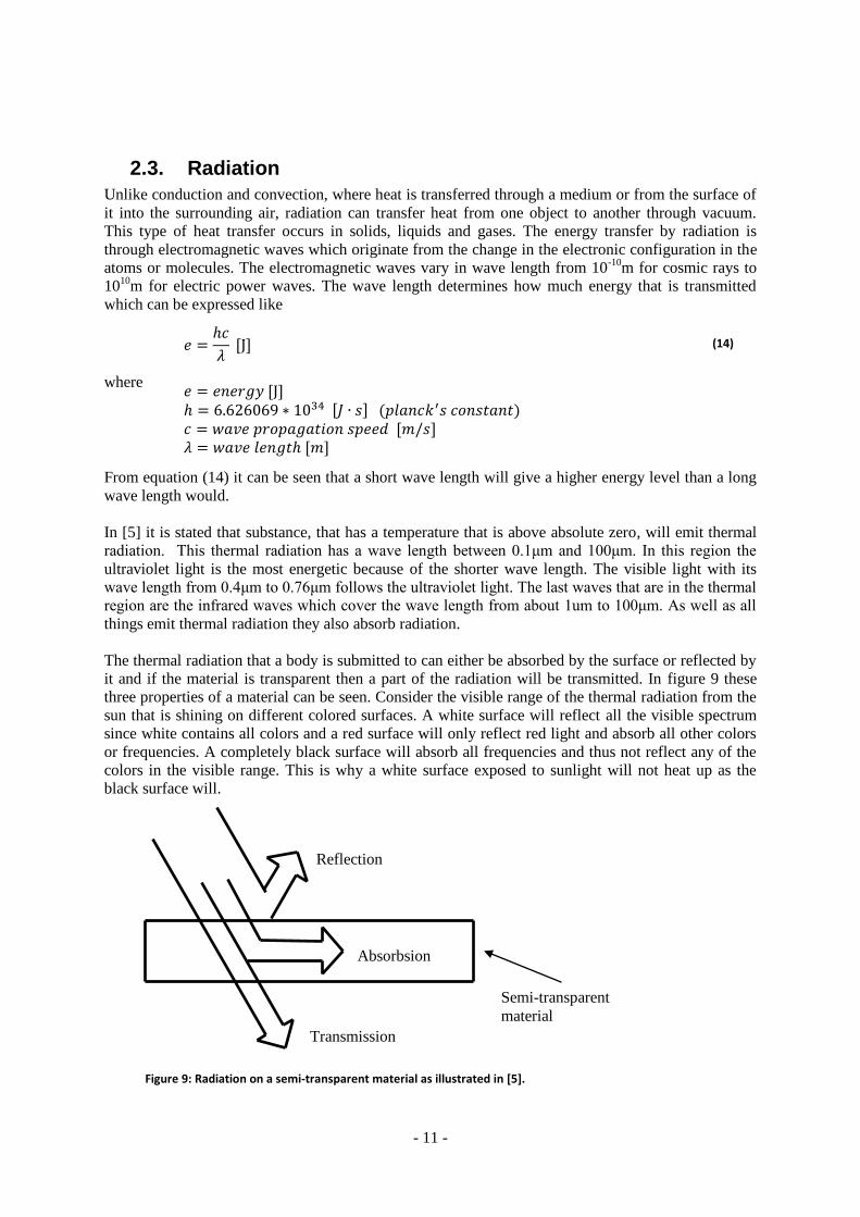
The thermal radiation that a body is submitted to can either be absorbed by the surface or reflected by
it and if the material is transparent then a part of the radiation will be transmitted. In figure 9 these
three properties of a material can be seen. Consider the visible range of the thermal radiation from the
sun that is shining on different colored surfaces. A white surface will reflect all the visible spectrum
since white contains all colors and a red surface will only reflect red light and absorb all other colors
or frequencies. A completely black surface will absorb all frequencies and thus not reflect any of the
colors in the visible range. This is why a white surface exposed to sunlight will not heat up as the
black surface will.
Semi-transparent
material
Reflection
Transmission
Absorbsion
Figure 9: Radiation on a semi-transparent material as illustrated in [5].

- 12 -
By using the Stefan-Boltzmann law the energy transfer by radiation can be determined as
(15)
where [ ] [ ] [ ] [ ]
[
]
The last coefficient determines how much of the emitted radiation from body A that is absorbed
by body B. To determine this coefficient for the two bodies knowledge of the bodies’ material is
needed with respect to how much radiation that is emitted and reflected. It is also important to know
the shape of the bodies to calculate how much they will influence each other since a curved surface
emit and reflect in a different way that a flat surface will. Besides from these calculations the
coefficient also consists of the Stefan-Boltzmann constant which according to [1] has been
determined through experiments to have the value .
2.3.1. Black Body
A black body is as described in [1] a body that appears black to the eye because it does not reflect any
radiation. It absorbs all incident radiation regardless of wavelength and direction. No surface can emit
more energy than a blackbody at specified temperature and wavelength. The emissive power of the
black body is in [2] expressed like
[ ] (16)
where the subscript b indicates that the emission is from a blackbody. It can be seen that the power
emitted is dependent on the temperature which is expressed in Kelvin. The blackbody is an idealized
body which serves as a standard for real surfaces so that their properties radiation can be evaluated.
2.3.2. Gray Body
The gray body is a body that is non black which means that almost all surfaces in real life are
considered gray. This is description is found in [2] where it furthermore is stated that surfaces will not
absorb all incident radiation but also reflect a part of it depending on the surface. The gray body has a
monochromatic emissivity that is independent of wavelength. This emissivity is a ratio between the
monochromatic emissive power of a gray body and the monochromatic emissive power of a
blackbody at the same wavelength and temperature. This relation is expressed in equation (17), and in
equation (18) and (19) the emissivity for both the gray and black body are stated respectively.
(17)
∫
[ ] (18)
∫
[ ] (19)
When doing calculations that involves several gray bodies the calculation get very complicated and
thus some simplifications are necessary. According to [1] it is normal to assume that the surfaces are
opaque, diffuse and gray. This means that the surfaces are non transparent, and that they are diffuse

- 13 -
emitters and reflectors which means that out going radiation is equally distributed in all directions.
The radiation properties are independent of wavelength, each of the surfaces are isothermal and both
the incoming and outgoing radiation are uniform over each surface.

- 14 -
3. Modeling in Simscape
Simscape is a physical modeling tool delivered by MathWorks as a toolbox to Simulink. For more
information, see [6]. The first release, version 1.0, came according to [7] together with Matlab
R2007a.
3.1. Physical Modeling – Simscape vs. Dymola
In order to understand Simscape it can for someone who is familiar with Dymola be convenient to
compare Dymola and Simscape. Both are physical modeling tools used to construct physical systems
containing components modeling physical elements, e.g. pumps and motors. The components are
connected using physical connections with units, see also [8] and [9].
Dymola is today delivered by Dassault Systèmes AB, Sweden that is a subsidiary company to
Dassault Systèmes that delivers CATIA. Thus, Dymola can, according to Wikipedia [10], be used by
itself or integrated in CATIA Systems V6. Dymola is, according to Dassault Systèmes themselves [8],
“the foundation technology for CATIA V6 Dynamic Behavior Modeling”. One of the basic ideas with
Dymola is, according to [8], the use of the object oriented modeling language, Modelica, which gives
the user freedom to create new or modify existing model libraries.
Simscape is, as mentioned before, also a physical modeling tool, but delivered by MathWorks as a
toolbox to Simulink. This gives the advantage that Simscape models can be integrated with Matlab,
Simulink and other products by MathWorks. In Simscape the Simscape language is used to define
custom components, see [9], in the same way as Dymola uses the Modelica language. As stated in
[21], the Simscape programming language is based on MATLAB object oriented language, in order to
be able to integrate it with the Simulink environment, not only when it comes to physical components,
but also areas of physics. The later refers to Simscape’s domains, covered in chapter 3.2.4.
The choice of which tool to use is not within the scope for the Master thesis work. It is already
specified in the assignment.
3.2. Differences between Simulink and Simscape Modeling
In this section, at first, the big differences between Simscape and Simulink modeling will be
explained. Then some of the properties that are special for Simscape are presented. Here “Simulink”
mainly refers to the basic Simulink library.
There are some distinct differences between Simulink and Simscape and they are as follows. Further
information can be found in [9] and [11]:
1. In Simulink mathematical operations are modeled, but in Simscape the model is constructed
by blocks representing physical components and physical relationships between them. It can
also be said that in Simulink the model is constructed by defining equations for the system,
but in Simscape the physical system with components is constructed and Simscape analyzes
and solves the equations that constitutes the system
2. The connections in Simulink are unitless and any block can be connected to any other block,
even if the simulation results become strange. In Simscape the connections represent physical
connections between components and they can have units. For example a voltage source can
be connected to a diode, but Simscape does not allow to connect a mass flow source to a
diode
- 15 -
3. The connections in Simscape are bidirectional. It means that e.g. the mass flow can be in a
positive or negative direction, depending on the pressure difference in the system. Compare to
Simulink where all connections are unidirectional
These three points can be explained from figure 16, showing a simple Simscape model with a
Constant Volume Pneumatic Chamber, but in order to understand the model some more information is
needed.
3.2.1. Heat Transfer in Simscape
Heat transfer by conduction, convection and radiation is in Simscape represented by Simscape’s
“Thermal Elements” described in this chapter. Common for all three elements are that they are
bidirectional, i.e. the heat transfer can occur in both directions and that they only consider one
dimensional heat transfer.
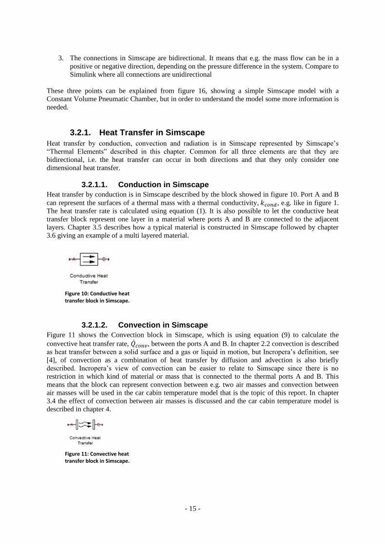
3.2.1.1. Conduction in Simscape
Heat transfer by conduction is in Simscape described by the block showed in figure 10. Port A and B
can represent the surfaces of a thermal mass with a thermal conductivity, , e.g. like in figure 1.
The heat transfer rate is calculated using equation (1). It is also possible to let the conductive heat
transfer block represent one layer in a material where ports A and B are connected to the adjacent
layers. Chapter 3.5 describes how a typical material is constructed in Simscape followed by chapter
3.6 giving an example of a multi layered material.
Figure 10: Conductive heat transfer block in Simscape.
3.2.1.2. Convection in Simscape
Figure 11 shows the Convection block in Simscape, which is using equation (9) to calculate the
convective heat transfer rate, , between the ports A and B. In chapter 2.2 convection is described
as heat transfer between a solid surface and a gas or liquid in motion, but Incropera’s definition, see
[4], of convection as a combination of heat transfer by diffusion and advection is also briefly
described. Incropera’s view of convection can be easier to relate to Simscape since there is no
restriction in which kind of material or mass that is connected to the thermal ports A and B. This
means that the block can represent convection between e.g. two air masses and convection between
air masses will be used in the car cabin temperature model that is the topic of this report. In chapter
3.4 the effect of convection between air masses is discussed and the car cabin temperature model is
described in chapter 4.
Figure 11: Convective heat transfer block in Simscape.
- 16 -
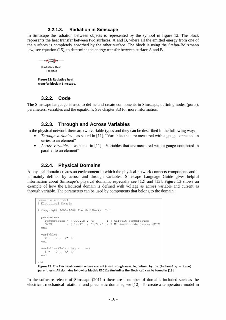
3.2.1.3. Radiation in Simscape
In Simscape the radiation between objects is represented by the symbol in figure 12. The block
represents the heat transfer between two surfaces, A and B, where all the emitted energy from one of
the surfaces is completely absorbed by the other surface. The block is using the Stefan-Boltzmann
law, see equation (15), to determine the energy transfer between surface A and B.
Figure 12: Radiative heat transfer block in Simscape.
3.2.2. Code
The Simscape language is used to define and create components in Simscape, defining nodes (ports),
parameters, variables and the equations. See chapter 3.3 for more information.
3.2.3. Through and Across Variables
In the physical network there are two variable types and they can be described in the following way:
Through variables – as stated in [11], “Variables that are measured with a gauge connected in
series to an element”
Across variables – as stated in [11], “Variables that are measured with a gauge connected in
parallel to an element”
3.2.4. Physical Domains
A physical domain creates an environment in which the physical network connects components and it
is mainly defined by across and through variables. Simscape Language Guide gives helpful
information about Simscape’s physical domains, especially see [12] and [13]. Figure 13 shows an
example of how the Electrical domain is defined with voltage as across variable and current as
through variable. The parameters can be used by components that belong to the domain.
domain electrical
% Electrical Domain
% Copyright 2005-2008 The MathWorks, Inc.
parameters
Temperature = { 300.15 , 'K' }; % Circuit temperature
GMIN = { 1e-12 , '1/Ohm' }; % Minimum conductance, GMIN
end
variables
v = { 0 , 'V' };
end
variables(Balancing = true)
i = { 0 , 'A' };
end
end
Figure 13: The Electrical domain where current ( ) is through variable, defined by the (Balancing = true) parenthesis. All domains following Matlab R2011a (including the Electrical) can be found in [13].
In the software release of Simscape (2011a) there are a number of domains included such as the
electrical, mechanical rotational and pneumatic domains, see [12]. To create a temperature model in

- 17 -
an enclosure with air inlets and outlets the Thermal and Pneumatic domains are convenient to use.
Their through and across variables are presented in table 3.
Table 3: Across and through variables in the Thermal and Pneumatic domain, according to [11]. Note that the Pneumatic domain has two Across and two Through variables
Domain Across variable Through
variable
Thermal Temperature Heat flow
Pneumatic Pressure
Temperature
Mass flow rate
Heat flow
As stated in [11], the across and through variables in a domain generally becomes power if they are
multiplied. The pneumatic domain has one exception, though. The product of pressure and mass flow
rate gives energy instead.
If the domains following Simscape are not enough, it is, according to [12], possible to create a new
domain and components belonging to it. The drawback with that is that the components can only be
connected to other components in the same domain.
3.2.5. Components
To learn how a new component is created, see chapter 3.3.
The components in Simscape are, alike Simulink represented with blocks and the Simscape block can
have the two following kinds of ports, see also [11] and [14]:
Physical Conserving ports are the physical connection ports. They can for example be
pneumatic or electrical. For physical conserving ports it holds that:
o The connections between them are bidirectional
o Each physical conserving port belongs to a domain and they can only be connected to
other physical conserving ports of the same domain
o The connection lines between them carry variables, cross and through variables
o Two conserving ports that are directly connected to each other must have the same
value on the across variable, e.g. angular velocity
o The connection lines from a physical conserving port can be branched into several
connections and the following happen with the through and across variables:
The components directly connected to each other must have the same value
on their cross variables
The value of the through variables are divided among the connections in the
branch and the sum of the incoming through variables is equal to the sum of
the outgoing ones
Physical Signal ports carry signals between blocks and their connections are more alike the
connections in Simulink, but using Simulink ports would slow down the computation speed.
For the physical signal ports it holds that:
o They can be connected to each other, bringing physical signals between Simscape
blocks
o The signals connecting them can have units, but only one unit per signal
o They can be connected to regular Simulink blocks using the Simulink-PS and PS-
Simulink Converters
Figure 14 shows a Controlled Pneumatic Flow Rate Source with physical conserving ports, A and B,
which are connected to other components within the Pneumatic domain. Normally an atmospheric
reference is connected to A, which means that the flow rate into A is zero. The physical signal port F

- 18 -
specifies how large the output flow rate should be or rather how large the difference between port A
and B should be.
Figure 14: Example of a component with physical conserving ports, A and B, and a physical signal port, F.
3.2.5.1. Connecting Physical Signals to Regular Simulink Components
The physical signals can be converted to regular unitless Simulink ports through a converter. There is
one converter for each direction, one for converting a Physical Signal to Simulink, see figure 16, and
one for converting a Simulink signal to a Physical Signal. In both cases the unit of the physical signal
can be specified in the block dialogs. The conversion to and from Simulink is especially useful when
using data as input from and output to the workspace, see also [11].
3.2.6. Example of a Simple Simscape Model
To give an example, the system described in figure 15(a) is constructed in Simscape. It is a tank filled
with air and it has a pipe directly to the atmosphere. There is an external heat flow source heating up
the tank and the enclosed air. This will be compared to the system in figure 15(b) where there is a
pump connected giving an air mass flow from into the tank.
(a) (b)
Figure 15: Example with a tank having a pipe to the atmosphere and a heat source
The Simscape model corresponding to the system in figure 15(a) is showed in figure 16 using a
Constant Volume Pneumatic Chamber to represent the tank. Some of its properties will be explained.
- 19 -
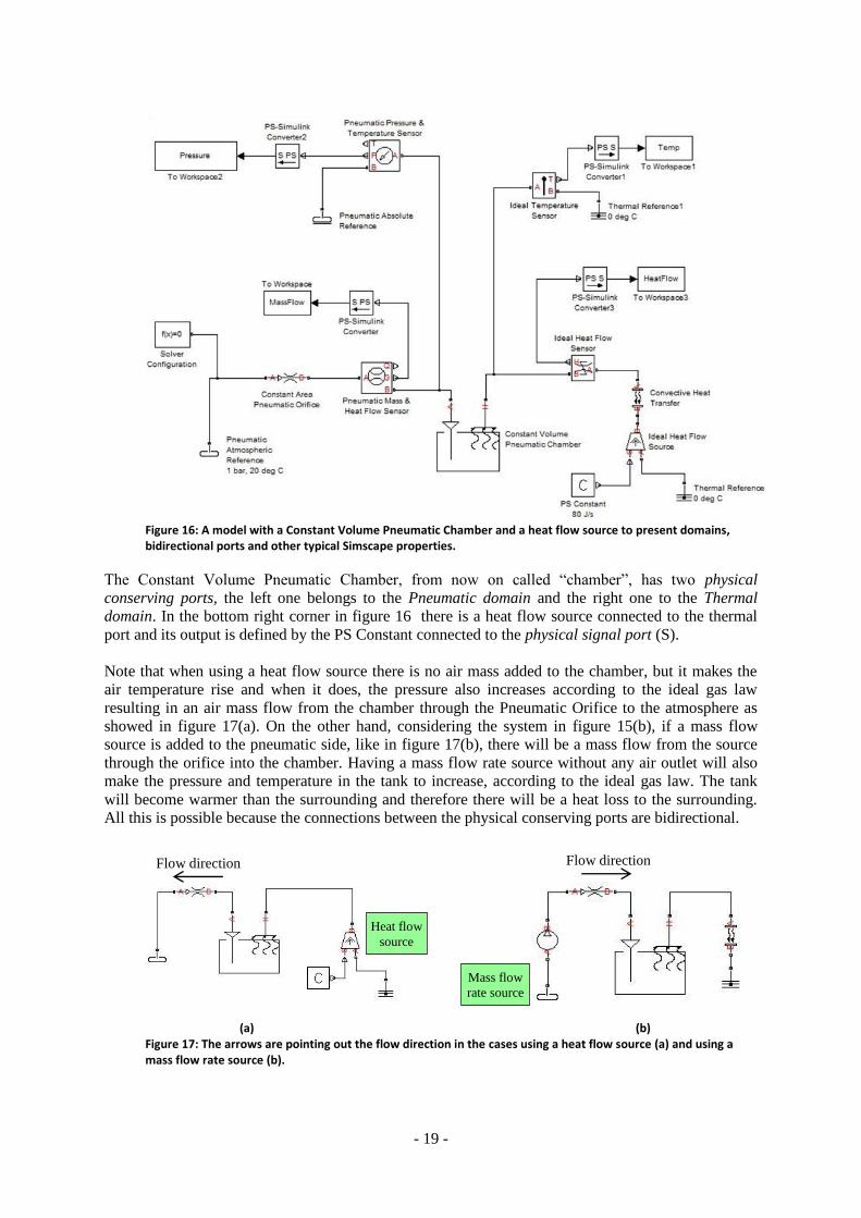
Figure 16: A model with a Constant Volume Pneumatic Chamber and a heat flow source to present domains, bidirectional ports and other typical Simscape properties.
The Constant Volume Pneumatic Chamber, from now on called “chamber”, has two physical
conserving ports, the left one belongs to the Pneumatic domain and the right one to the Thermal
domain. In the bottom right corner in figure 16 there is a heat flow source connected to the thermal
port and its output is defined by the PS Constant connected to the physical signal port (S).
Note that when using a heat flow source there is no air mass added to the chamber, but it makes the
air temperature rise and when it does, the pressure also increases according to the ideal gas law
resulting in an air mass flow from the chamber through the Pneumatic Orifice to the atmosphere as
showed in figure 17(a). On the other hand, considering the system in figure 15(b), if a mass flow
source is added to the pneumatic side, like in figure 17(b), there will be a mass flow from the source
through the orifice into the chamber. Having a mass flow rate source without any air outlet will also
make the pressure and temperature in the tank to increase, according to the ideal gas law. The tank
will become warmer than the surrounding and therefore there will be a heat loss to the surrounding.
All this is possible because the connections between the physical conserving ports are bidirectional.
(a) (b) Figure 17: The arrows are pointing out the flow direction in the cases using a heat flow source (a) and using a mass flow rate source (b).
Mass flow
rate source
Heat flow
source
Flow direction Flow direction
- 20 -
Regarding through- and across variables it is easy to see in figure 16 that the sensors for through
variables are placed in series with the connections and for across variables they are connected in
parallel. The outputs from the sensors are physical signals and connected to Physical Signal to
Simulink Converters in order to bring the result to Matlab’s workspace.
3.3. Creating a Custom Component in Simscape
The domains in Simscape include several different components for construction of physical systems
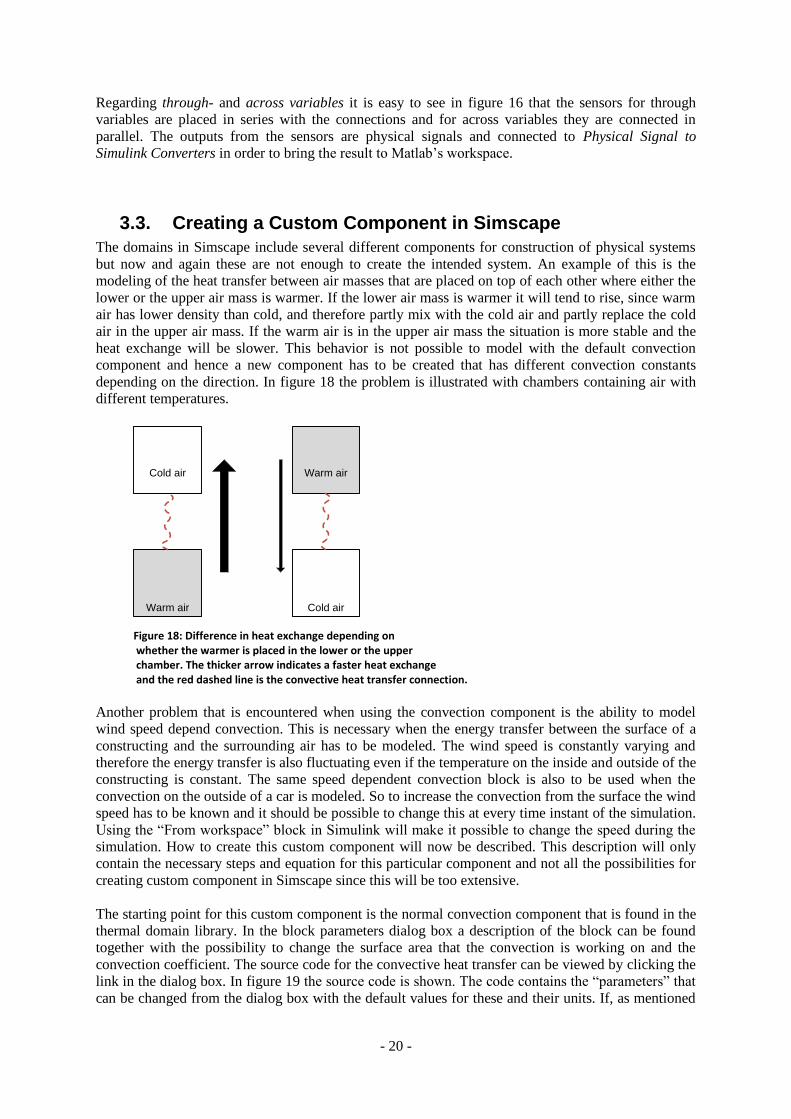
but now and again these are not enough to create the intended system. An example of this is the
modeling of the heat transfer between air masses that are placed on top of each other where either the
lower or the upper air mass is warmer. If the lower air mass is warmer it will tend to rise, since warm
air has lower density than cold, and therefore partly mix with the cold air and partly replace the cold
air in the upper air mass. If the warm air is in the upper air mass the situation is more stable and the
heat exchange will be slower. This behavior is not possible to model with the default convection
component and hence a new component has to be created that has different convection constants
depending on the direction. In figure 18 the problem is illustrated with chambers containing air with
different temperatures.
Warm air
Warm air
Cold air
Cold air
Figure 18: Difference in heat exchange depending on whether the warmer is placed in the lower or the upper chamber. The thicker arrow indicates a faster heat exchange and the red dashed line is the convective heat transfer connection.
Another problem that is encountered when using the convection component is the ability to model
wind speed depend convection. This is necessary when the energy transfer between the surface of a
constructing and the surrounding air has to be modeled. The wind speed is constantly varying and
therefore the energy transfer is also fluctuating even if the temperature on the inside and outside of the
constructing is constant. The same speed dependent convection block is also to be used when the
convection on the outside of a car is modeled. So to increase the convection from the surface the wind
speed has to be known and it should be possible to change this at every time instant of the simulation.
Using the “From workspace” block in Simulink will make it possible to change the speed during the
simulation. How to create this custom component will now be described. This description will only
contain the necessary steps and equation for this particular component and not all the possibilities for
creating custom component in Simscape since this will be too extensive.
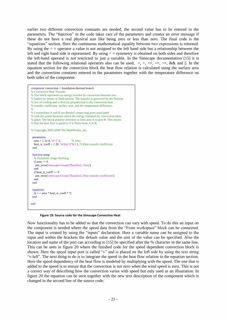
The starting point for this custom component is the normal convection component that is found in the
thermal domain library. In the block parameters dialog box a description of the block can be found
together with the possibility to change the surface area that the convection is working on and the
convection coefficient. The source code for the convective heat transfer can be viewed by clicking the
link in the dialog box. In figure 19 the source code is shown. The code contains the “parameters” that
can be changed from the dialog box with the default values for these and their units. If, as mentioned
- 21 -
earlier two different convection constants are needed, the second value has to be entered in the
parameters. The “function” in the code takes care of the parameters and creates an error message if
these do not have a real physical size like being zero or less than zero. The final code is the
“equations” section. Here the continuous mathematical equality between two expressions is returned.
By using the = = operator a value is not assigned to the left hand side but a relationship between the
left and right hand side is represented. By using = = symmetry is obtained on both sides and therefore
the left-hand operand is not restricted to just a variable. In the Simscape documentation [15] it is
stated that the following relational operators also can be used, <, >, <=, >=, ~=, && and ||. In the
equation section for the convection block the heat flow relation is calculated using the surface area
and the convection constants entered in the parameters together with the temperature difference on
both sides of the component.
Now functionality has to be added so that the convection can vary with speed. To do this an input on
the component is needed where the speed data from the “From workspace” block can be connected.
The input is created by using the “inputs” declaration. Here a variable name can be assigned to the
input and within the brackets the default value and the unit of the value can be specified. Also the
location and name of the port can according to [15] be specified after the % character in the same line.
This can be seen in figure 20 where the finished code for the speed dependent convection block is
shown. Here the speed input port is called “v” and is placed on the left side by using the text string
“v:left”. The next thing to do is to integrate the speed in the heat flow relation in the equation section.
Here the speed dependency of the heat flow is modeled by multiplying with the speed. The one that is
added to the speed is to ensure that the convection is not zero when the wind speed is zero. This is not
a correct way of describing how the convection varies with speed but only used as an illustration. In
figure 20 the equation can be seen together with the new text description of the component which is
changed in the second line of the source code.
component convection < foundation.thermal.branch
% Convective Heat Transfer % The block represents an energy transfer by convection between two
% bodies by means of fluid motion. The transfer is governed by the Newton
% law of cooling and is directly proportional to the convection heat % transfer coefficient, surface area, and the temperature difference.
%
% Connections A and B are thermal conserving ports associated % with the points between which the energy transport by convection takes
% place. The block positive direction is from port A to port B. This means
% that the heat flow is positive if it flows from A to B.
% Copyright 2005-2008 The MathWorks, Inc.
parameters
area = { 1e-4, 'm^2' }; % Area
heat_tr_coeff = { 20, 'W/(m^2*K)' }; % Heat transfer coefficient
end
function setup % Parameter range checking
if area <= 0
pm_error('simscape:GreaterThanZero','Area') end
if heat_tr_coeff <= 0
pm_error('simscape:GreaterThanZero','Heat transfer coefficient') end
end
equations
Q = = area * heat_tr_coeff * T;
end
end
Figure 19: Source code for the Simscape Convective Heat

- 22 -
When changing or creating new code for a component it has to be saved as an .ssc-file, and it cannot
be used before it is built using the Matlab command “ssc_build” followed by the folder name where
the file is saved. The resulting component is shown in figure 21 where it can be seen that it is
transformed into a block without an icon as the original. To get the original or a custom icon on the
component an image has to be placed in the same folder as the code with exactly the same name as
the file containing the code. This image file can either be of the type jpg, bmp or png. In figure 21 the
final speed dependent convection component is shown with the old convection icon but with the extra
speed input port.
The changes performed here are only a small part of what can be done with the Simscape language
and in the MathWorks help files a comprehensive description of all possibilities can be found. Finally
the result of the speed dependency can be seen in figure 22 together with the original convection
component convection_Speed < foundation.thermal.branch
% Convective Heat Transfer - Speed Dependent % The block represents an energy transfer by convection between two
% bodies by means of fluid motion. The transfer is governed by the Newton
% law of cooling and is directly proportional to the convection heat % transfer coefficient, surface area, and the temperature difference.
%
% Connections A and B are thermal conserving ports associated % with the points between which the energy transport by convection takes
% place. The block positive direction is from port A to port B. This means
% that the heat flow is positive if it flows from A to B.
% Copyright 2005-2008 The MathWorks, Inc.
inputs
speed = 0 ; % v:left end
parameters area = { 1e-4, 'm^2' }; % Area
heat_tr_coeff = { 20, 'W/(m^2*K)' }; % Heat transfer coefficient
end
function setup
% Parameter range checking if area <= 0
pm_error('simscape:GreaterThanZero','Area')
end if heat_tr_coeff <= 0
pm_error('simscape:GreaterThanZero','Heat transfer coefficient')
end end
equations Q == area * heat_tr_coeff * T * (1+speed);
end
end
Figure 21: Convection heat transfer components, original, custom and custom with icon.
Figure 20: Code for the speed dependent convection component.
- 23 -
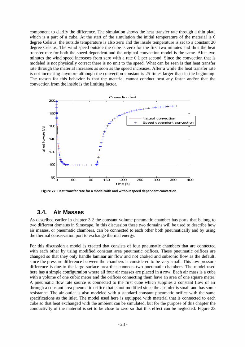
component to clarify the difference. The simulation shows the heat transfer rate through a thin plate
which is a part of a cube. At the start of the simulation the initial temperature of the material is 0
degree Celsius, the outside temperature is also zero and the inside temperature is set to a constant 20
degree Celsius. The wind speed outside the cube is zero for the first two minutes and thus the heat
transfer rate for both the speed dependent and the original convection model is the same. After two
minutes the wind speed increases from zero with a rate 0.1 per second. Since the convection that is
modeled is not physically correct there is no unit to the speed. What can be seen is that heat transfer
rate through the material increases as soon as the speed increases. After a while the heat transfer rate
is not increasing anymore although the convection constant is 25 times larger than in the beginning.
The reason for this behavior is that the material cannot conduct heat any faster and/or that the
convection from the inside is the limiting factor.
Figure 22: Heat transfer rate for a model with and without speed dependent convection.
3.4. Air Masses
As described earlier in chapter 3.2 the constant volume pneumatic chamber has ports that belong to
two different domains in Simscape. In this discussion these two domains will be used to describe how
air masses, or pneumatic chambers, can be connected to each other both pneumatically and by using
the thermal conservation port to exchange thermal energy.
For this discussion a model is created that consists of four pneumatic chambers that are connected
with each other by using modified constant area pneumatic orifices. These pneumatic orifices are
changed so that they only handle laminar air flow and not choked and subsonic flow as the default,
since the pressure difference between the chambers is considered to be very small. This low pressure
difference is due to the large surface area that connects two pneumatic chambers. The model used
here has a simple configuration where all four air masses are placed in a row. Each air mass is a cube
with a volume of one cubic meter and the orifices connecting them have an area of one square meter.
A pneumatic flow rate source is connected to the first cube which supplies a constant flow of air
through a constant area pneumatic orifice that is not modified since the air inlet is small and has some
resistance. The air outlet is also modeled with a standard constant pneumatic orifice with the same
specifications as the inlet. The model used here is equipped with material that is connected to each
cube so that heat exchanged with the ambient can be simulated, but for the purpose of this chapter the
conductivity of the material is set to be close to zero so that this effect can be neglected. Figure 23
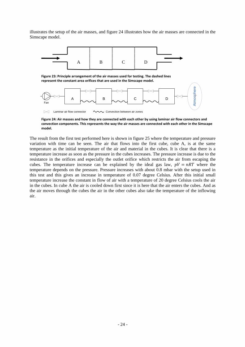
- 24 -
illustrates the setup of the air masses, and figure 24 illustrates how the air masses are connected in the
Simscape model.
Fan
A B C D
Laminar air flow connector Convection between air zones
Atm
osp
he
re
Figure 24: Air masses and how they are connected with each other by using laminar air flow connectors and convection components. This represents the way the air masses are connected with each other in the Simscape model.
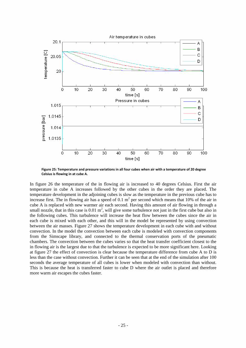
The result from the first test performed here is shown in figure 25 where the temperature and pressure
variation with time can be seen. The air that flows into the first cube, cube A, is at the same
temperature as the initial temperature of the air and material in the cubes. It is clear that there is a
temperature increase as soon as the pressure in the cubes increases. The pressure increase is due to the
resistance in the orifices and especially the outlet orifice which restricts the air from escaping the
cubes. The temperature increase can be explained by the ideal gas law, where the
temperature depends on the pressure. Pressure increases with about 0.8 mbar with the setup used in
this test and this gives an increase in temperature of 0.07 degree Celsius. After this initial small
temperature increase the constant in flow of air with a temperature of 20 degree Celsius cools the air
in the cubes. In cube A the air is cooled down first since it is here that the air enters the cubes. And as
the air moves through the cubes the air in the other cubes also take the temperature of the inflowing
air.
A B C D
Figure 23: Principle arrangement of the air masses used for testing. The dashed lines represent the constant area orifices that are used in the Simscape model.
- 25 -
Figure 25: Temperature and pressure variations in all four cubes when air with a temperature of 20 degree Celsius is flowing in at cube A.
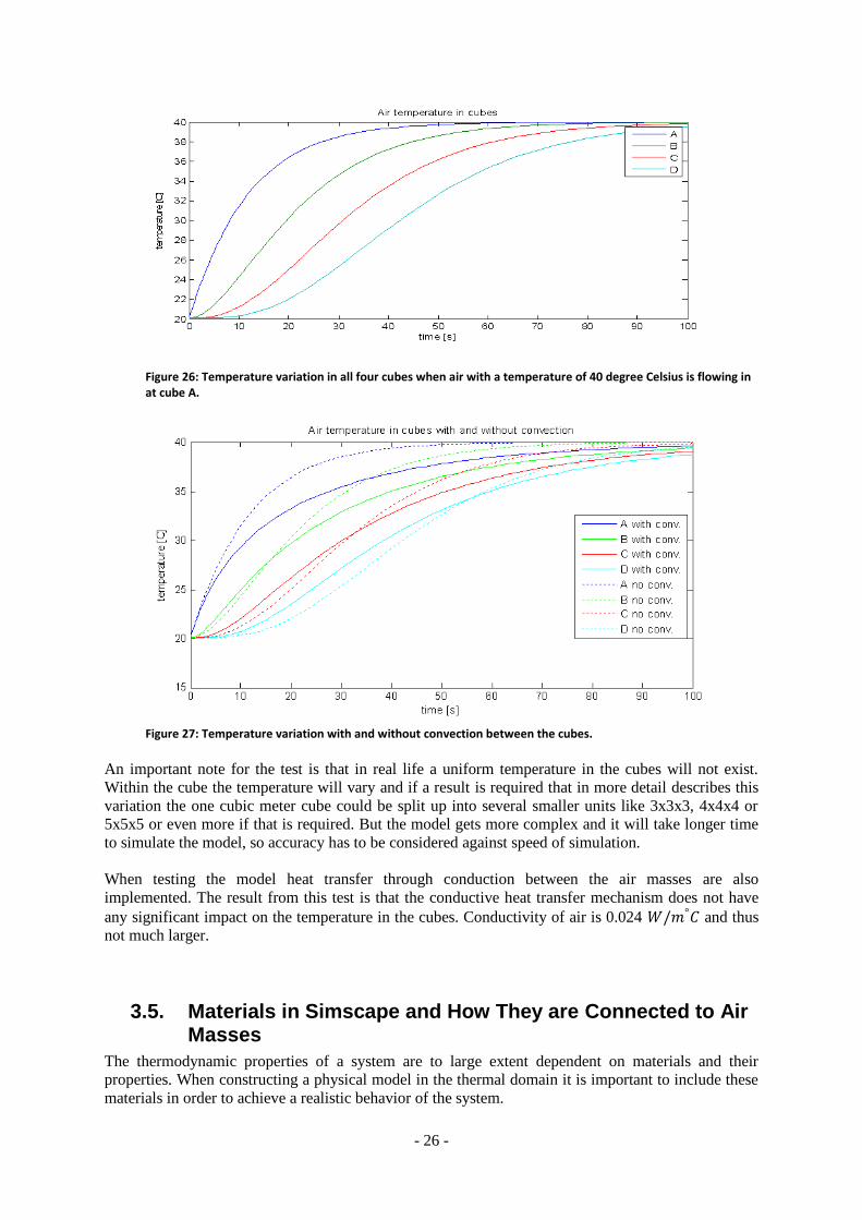
In figure 26 the temperature of the in flowing air is increased to 40 degrees Celsius. First the air
temperature in cube A increases followed by the other cubes in the order they are placed. The
temperature development in the adjoining cubes is slow as the temperature in the previous cube has to
increase first. The in flowing air has a speed of 0.1 m2 per second which means that 10% of the air in
cube A is replaced with new warmer air each second. Having this amount of air flowing in through a
small nozzle, that in this case is 0.01 m2, will give some turbulence not just in the first cube but also in
the following cubes. This turbulence will increase the heat flow between the cubes since the air in
each cube is mixed with each other, and this will in the model be represented by using convection
between the air masses. Figure 27 shows the temperature development in each cube with and without
convection. In the model the convection between each cube is modeled with convection components
from the Simscape library, and connected to the thermal conservation ports of the pneumatic
chambers. The convection between the cubes varies so that the heat transfer coefficient closest to the
in flowing air is the largest due to that the turbulence is expected to be more significant here. Looking
at figure 27 the effect of convection is clear because the temperature difference from cube A to D is
less than the case without convection. Further it can be seen that at the end of the simulation after 100
seconds the average temperature of all cubes is lower when modeled with convection than without.
This is because the heat is transferred faster to cube D where the air outlet is placed and therefore
more warm air escapes the cubes faster.
- 26 -
Figure 26: Temperature variation in all four cubes when air with a temperature of 40 degree Celsius is flowing in at cube A.
Figure 27: Temperature variation with and without convection between the cubes.
An important note for the test is that in real life a uniform temperature in the cubes will not exist.
Within the cube the temperature will vary and if a result is required that in more detail describes this
variation the one cubic meter cube could be split up into several smaller units like 3x3x3, 4x4x4 or
5x5x5 or even more if that is required. But the model gets more complex and it will take longer time
to simulate the model, so accuracy has to be considered against speed of simulation.
When testing the model heat transfer through conduction between the air masses are also
implemented. The result from this test is that the conductive heat transfer mechanism does not have
any significant impact on the temperature in the cubes. Conductivity of air is 0.024 and thus
not much larger.
3.5. Materials in Simscape and How They are Connected to Air Masses
The thermodynamic properties of a system are to large extent dependent on materials and their
properties. When constructing a physical model in the thermal domain it is important to include these
materials in order to achieve a realistic behavior of the system.
- 27 -
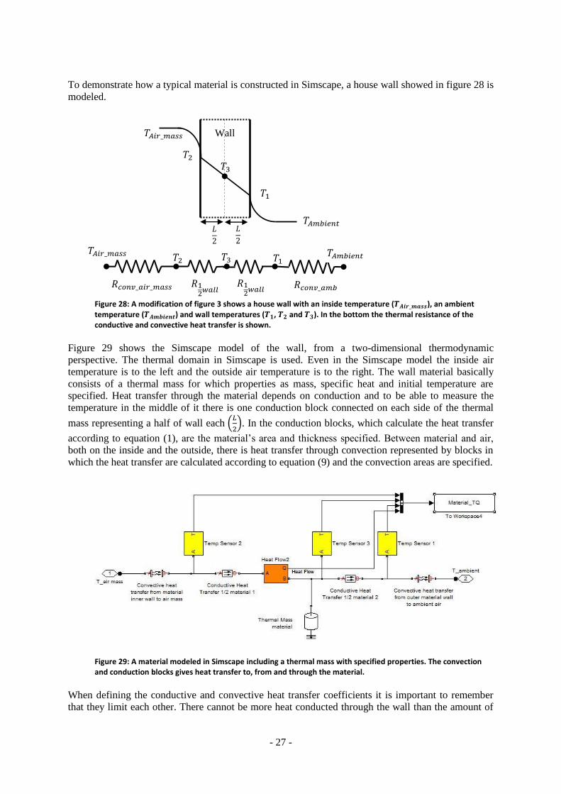
To demonstrate how a typical material is constructed in Simscape, a house wall showed in figure 28 is
modeled.
Figure 28: A modification of figure 3 shows a house wall with an inside temperature ( ), an ambient temperature ( ) and wall temperatures ( , and ). In the bottom the thermal resistance of the conductive and convective heat transfer is shown.
Figure 29 shows the Simscape model of the wall, from a two-dimensional thermodynamic
perspective. The thermal domain in Simscape is used. Even in the Simscape model the inside air
temperature is to the left and the outside air temperature is to the right. The wall material basically
consists of a thermal mass for which properties as mass, specific heat and initial temperature are
specified. Heat transfer through the material depends on conduction and to be able to measure the
temperature in the middle of it there is one conduction block connected on each side of the thermal
mass representing a half of wall each (
). In the conduction blocks, which calculate the heat transfer
according to equation (1), are the material’s area and thickness specified. Between material and air,
both on the inside and the outside, there is heat transfer through convection represented by blocks in
which the heat transfer are calculated according to equation (9) and the convection areas are specified.
Figure 29: A material modeled in Simscape including a thermal mass with specified properties. The convection and conduction blocks gives heat transfer to, from and through the material.
When defining the conductive and convective heat transfer coefficients it is important to remember
that they limit each other. There cannot be more heat conducted through the wall than the amount of
Wall
- 28 -
heat reaching the wall through convection, or there cannot be more heat transported away from the
wall by convection, than is transported through the wall by conduction.
In figure 29 three temperature sensors are placed measuring the temperature on both surfaces and in
the middle of the material. Also a heat flow sensor measures the total heat flow through the material.
3.6. Comparison of Multi Layer Material and a Single Layer Material Model
To avoid that a model gets to complicated and therefore will require too much computing power it is
necessary to investigate if a simplification of a part in the model will change the result significantly.
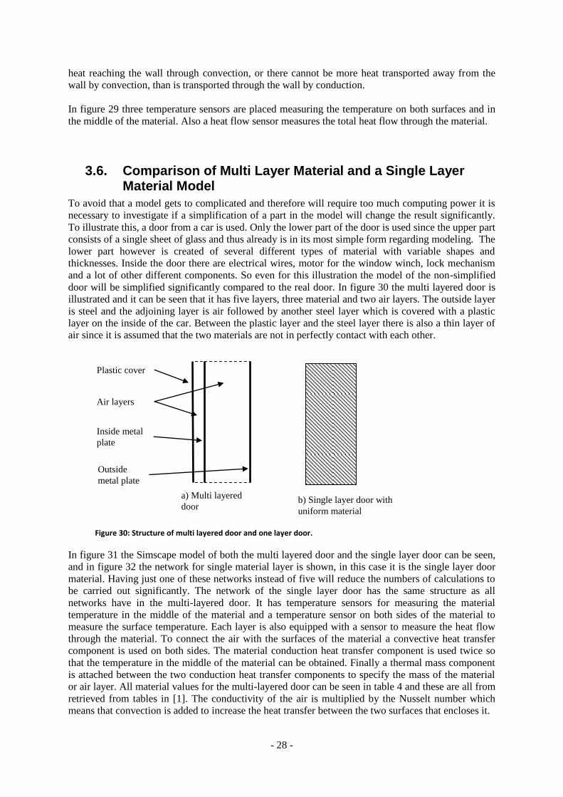
To illustrate this, a door from a car is used. Only the lower part of the door is used since the upper part
consists of a single sheet of glass and thus already is in its most simple form regarding modeling. The
lower part however is created of several different types of material with variable shapes and
thicknesses. Inside the door there are electrical wires, motor for the window winch, lock mechanism
and a lot of other different components. So even for this illustration the model of the non-simplified
door will be simplified significantly compared to the real door. In figure 30 the multi layered door is
illustrated and it can be seen that it has five layers, three material and two air layers. The outside layer
is steel and the adjoining layer is air followed by another steel layer which is covered with a plastic
layer on the inside of the car. Between the plastic layer and the steel layer there is also a thin layer of
air since it is assumed that the two materials are not in perfectly contact with each other.
In figure 31 the Simscape model of both the multi layered door and the single layer door can be seen,
and in figure 32 the network for single material layer is shown, in this case it is the single layer door
material. Having just one of these networks instead of five will reduce the numbers of calculations to
be carried out significantly. The network of the single layer door has the same structure as all
networks have in the multi-layered door. It has temperature sensors for measuring the material
temperature in the middle of the material and a temperature sensor on both sides of the material to
measure the surface temperature. Each layer is also equipped with a sensor to measure the heat flow
through the material. To connect the air with the surfaces of the material a convective heat transfer
component is used on both sides. The material conduction heat transfer component is used twice so
that the temperature in the middle of the material can be obtained. Finally a thermal mass component
is attached between the two conduction heat transfer components to specify the mass of the material
or air layer. All material values for the multi-layered door can be seen in table 4 and these are all from
retrieved from tables in [1]. The conductivity of the air is multiplied by the Nusselt number which
means that convection is added to increase the heat transfer between the two surfaces that encloses it.
b) Single layer door with
uniform material
Plastic cover
Air layers
Outside
metal plate
Inside metal
plate
a) Multi layered
door
Figure 30: Structure of multi layered door and one layer door.
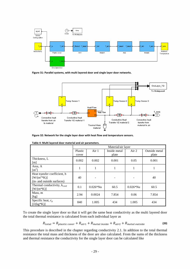
- 29 -
Figure 31: Parallel systems, with multi layered door and single layer door networks.
Figure 32: Network for the single layer door with heat flow and temperature sensors.
Table 4: Multi layered door material and air parameters.
Material/air layer
Plastic
cover
Air 1 Inside metal
plate
Air 2 Outside metal
plate
Thickness, L
[m] 0.002 0.002 0.001 0.05 0.001
Area, A
[m2]
1 1 1 1 1
Heat transfer coefficient, h
[W/(m2*K)]
(in- and outside surfaces)
40 - - - 40
Thermal conductivity, kcond
[W/(m*K)] 0.1 0.026*Nu 60.5 0.026*Nu 60.5
Mass, m
[kg] 2.94 0.0024 7.854 0.06 7.854
Specific heat, cp
[J/(kg*K)] 840 1.005 434 1.005 434
To create the single layer door so that it will get the same heat conductivity as the multi layered door
the total thermal resistance is calculated from each individual layer as
(20)
This procedure is described in the chapter regarding conductivity 2.1. In addition to the total thermal
resistance the total mass and thickness of the door are also calculated. From the sums of the thickness
and thermal resistance the conductivity for the single layer door can be calculated like

- 30 -
(21)
The specific heat of the single layer material can be determined by calculating the sum of each
individual heat capacity of the layers and then divide this by the total mass of the layers as
(
) (22)
Now a material that has the same heat flow rate as the multi layered door is created and the values for
the single layer door are presented in table 5. However, this is only true for steady state conditions but
not for transient conditions as can be seen in figure 33. The result from figure 33 is obtained by giving
both doors an initial temperature of zero degree Celsius and then exposing them to an outside
temperature of zero degree Celsius and an inside temperature of 20 degree Celsius which will give a
temperature difference across the doors of 20 degrees. Positive heat flow rate is from the inside to the
outside. From figure 33 a big difference in the behavior of the materials can be observed with the
plastic cover having the largest initial heat flow rate. This is due to the large temperature difference in
the start and that the plastic cover is very thin. A thin material will give a faster heat transfer rate in
the simulation done here since the heat flow sensor is placed in the middle of the material. When
energy is transferred through the plastic cover and the first of the two air layers the inside metal plate
also transfers energy to the second air layer. The metal plate can also transfer heat fast since the metal
has a good ability to conduct. So compared to the single layer system steady state conditions are
attained faster due to having the most of the mass concentrated in the 3 material layers.
Table 5: Parameters for single layer door.
Thickness, L
[m] 0.0560
Area, A
[m2]
1
Heat transfer coefficient, h
[W/(m2*K)]
(in- and outside surfaces)
40
Thermal conductivity, kcond
[W/(m*K)] 0.0815
Mass, m
[kg] 18.71
Specific heat , cp
[J/(kg*K)] 496.35
The single layer material has low heat conductivity but also a high specific heat capacity which means
that it takes longer time to transport heat into the material. The high specific heat capacity delays the
heat flow through the material since a lot of energy is used to warm up the material. Also when
looking at figure 33 it is clear to see that the multi layered door has very different temperatures for
each of the layers. Especially it can be seen that the outside metal plate has a very low temperature,
less than one degree, because it is insulated from the inside metal plate by a layer of air which is a
good insulator. Therefore less energy is needed to heat up the material than is the case with the single
layer material. In figure 34 it can also be seen that for the single layer system the temperatures on the
surfaces are close to those of the multi layered system but with some delay. In figure 35(a) a
sinusoidal wave is added to the outside temperature which makes it vary between -10 and +10 with a
period time of one hour. The figure shows how the temperature makes the material and air in both
doors vary with time. The most interesting temperature for the modeling purpose is the inside surface
temperature and how it will affect the air temperature. To see how this temperature varies a
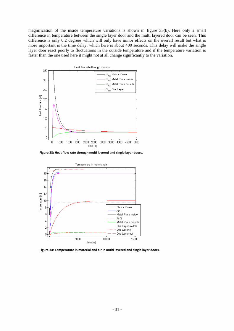
- 31 -
magnification of the inside temperature variations is shown in figure 35(b). Here only a small
difference in temperature between the single layer door and the multi layered door can be seen. This
difference is only 0.2 degrees which will only have minor effects on the overall result but what is
more important is the time delay, which here is about 400 seconds. This delay will make the single
layer door react poorly to fluctuations in the outside temperature and if the temperature variation is
faster than the one used here it might not at all change significantly to the variation.
Figure 33: Heat flow rate through multi layered and single layer doors.
Figure 34: Temperature in material and air in multi layered and single layer doors.
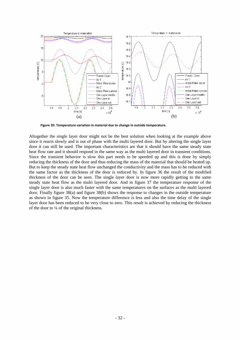
- 32 -
Altogether the single layer door might not be the best solution when looking at the example above
since it reacts slowly and is out of phase with the multi layered door. But by altering the single layer
door it can still be used. The important characteristics are that it should have the same steady state
heat flow rate and it should respond in the same way as the multi layered door in transient conditions.
Since the transient behavior is slow this part needs to be speeded up and this is done by simply
reducing the thickness of the door and thus reducing the mass of the material that should be heated up.
But to keep the steady state heat flow unchanged the conductivity and the mass has to be reduced with
the same factor as the thickness of the door is reduced by. In figure 36 the result of the modified
thickness of the door can be seen. The single layer door is now more rapidly getting to the same
steady state heat flow as the multi layered door. And in figure 37 the temperature response of the
single layer door is also much faster with the same temperatures on the surfaces as the multi layered
door. Finally figure 38(a) and figure 38(b) shows the response to changes in the outside temperature
as shown in figure 35. Now the temperature difference is less and also the time delay of the single
layer door has been reduced to be very close to zero. This result is achieved by reducing the thickness
of the door to ¼ of the original thickness.
(a) (b)
Figure 35: Temperature variation in material due to change in outside temperature.
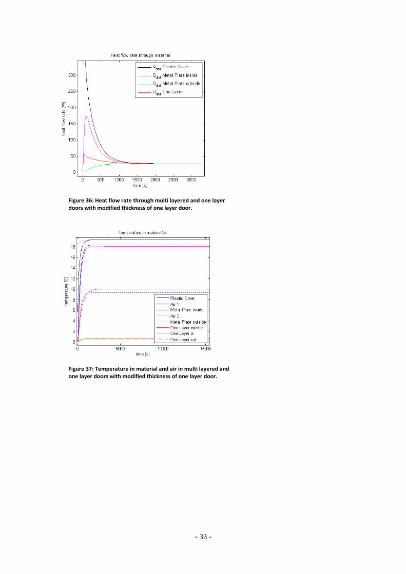
- 33 -
Figure 36: Heat flow rate through multi layered and one layer doors with modified thickness of one layer door.
Figure 37: Temperature in material and air in multi layered and one layer doors with modified thickness of one layer door.
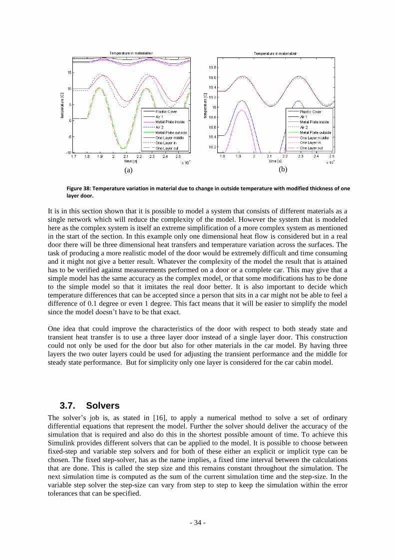
- 34 -
It is in this section shown that it is possible to model a system that consists of different materials as a
single network which will reduce the complexity of the model. However the system that is modeled
here as the complex system is itself an extreme simplification of a more complex system as mentioned
in the start of the section. In this example only one dimensional heat flow is considered but in a real
door there will be three dimensional heat transfers and temperature variation across the surfaces. The
task of producing a more realistic model of the door would be extremely difficult and time consuming
and it might not give a better result. Whatever the complexity of the model the result that is attained
has to be verified against measurements performed on a door or a complete car. This may give that a
simple model has the same accuracy as the complex model, or that some modifications has to be done
to the simple model so that it imitates the real door better. It is also important to decide which
temperature differences that can be accepted since a person that sits in a car might not be able to feel a
difference of 0.1 degree or even 1 degree. This fact means that it will be easier to simplify the model
since the model doesn’t have to be that exact.
One idea that could improve the characteristics of the door with respect to both steady state and
transient heat transfer is to use a three layer door instead of a single layer door. This construction
could not only be used for the door but also for other materials in the car model. By having three
layers the two outer layers could be used for adjusting the transient performance and the middle for
steady state performance. But for simplicity only one layer is considered for the car cabin model.
3.7. Solvers
The solver’s job is, as stated in [16], to apply a numerical method to solve a set of ordinary
differential equations that represent the model. Further the solver should deliver the accuracy of the
simulation that is required and also do this in the shortest possible amount of time. To achieve this
Simulink provides different solvers that can be applied to the model. It is possible to choose between
fixed-step and variable step solvers and for both of these either an explicit or implicit type can be
chosen. The fixed step-solver, has as the name implies, a fixed time interval between the calculations
that are done. This is called the step size and this remains constant throughout the simulation. The
next simulation time is computed as the sum of the current simulation time and the step-size. In the
variable step solver the step-size can vary from step to step to keep the simulation within the error
tolerances that can be specified.
(a) (b)
Figure 38: Temperature variation in material due to change in outside temperature with modified thickness of one layer door.
- 35 -
Whether to choose the fixed step or the variable step solver depends according to [16] on different
factors. If the model is to be implemented in a real-time system a fixed step solver should be chosen
to simulate the model since the variable step size cannot be mapped to the real time clock. But since
the fixed step size can give long simulation times, when the simulation time is large, a variable step
solver might be desirable during development and testing because it can shorten the simulation time
significantly. This time saving is obtained by reducing the number of steps and thus increasing the
step size. This can be done when the simulation result is within the error tolerance specified.
From [16] it is found that the implicit or explicit solver type is to be chosen from knowledge of the
stiffness of the model. A model is said to be stiff if the system has extremely different time scales.
The explicit solvers are the best choice for systems that are non-stiff, consequently having small
differences in time scale, and the implicit solvers are designed for solving stiff problems. The implicit
solvers are more stable when having oscillatory behavior in the system, but they will also be more
computationally expensive.
3.7.1. Choosing a Solver for Simscape
For physical models such as Simscape models MathWorks [17] recommends implicit solvers since
these require fewer time steps than explicit solvers. Simscape models are typically considered stiff
and therefore the explicit solvers cannot be used or are at least not recommended.
It is also possible to work with a global solver for the entire Simulink model and a local solver in each
Simscape part according to [18]. The idea is that different solvers are applied to different Simscape
systems so that an implicit solver is used on stiff parts and explicit solvers on non-stiff parts. The
benefit from this approach is that the simulation becomes more efficient and will reduce the
computational cost.
Another approach found in [18] is to use local fixed step solvers for each Simscape part and continue
to use a variable step global solver for the entire Simulink model. This can be done through the Solver
configuration block that must be added to each Simscape network. Here the choice is between the
default Backward Euler and the Trapezoidal Rule. If the local fixed step solver is used then the global
solver will treat this network as having discrete states. Other networks might not use this option and
some Simulink or non Simscape parts of the model might have continuous states and therefore the
global solver has to be continuous too. Only if all parts of the model have discrete states the global
solver can be a discrete.
3.7.2. Solver Choice for a Simscape Model and Tests
When starting testing on a Simscape model that included both air-masses and material which are
connected to each other either from air to air or from air to material it became clear that simulation
time is dependent on how the settings in the system is made with respect to the values of the
convection components. A high value of these components will increase the heat exchange between
the air masses and/or air masses and material. This means that the system becomes stiffer and thus
more difficult to simulate. The result when increasing the convection parameters to high values is that
the simulation halted before the intended completion time. A warning is given in the workspace that
the solver is unable to reduce step size without violating the minimum step size due to among others
the high stiffness of the system. In [20] it is stated that a variable step solver dynamically adjusts the
step size to be very small when the behavior of the system changes fast to improve accuracy. But the
technique that is used by the Simulink software to locate a discontinuity without having to use to
small time steps and thereby increase simulation time, called zero crossing detection, can also cause
the simulation to halt altogether.
So to be able to simulate the model a fixed time local solver is to be used instead of the variable step
solver. This means that the simulation time will hugely depend on the step size that is defined for the
local solver. And since simulation times of several hours are planned when testing the model for
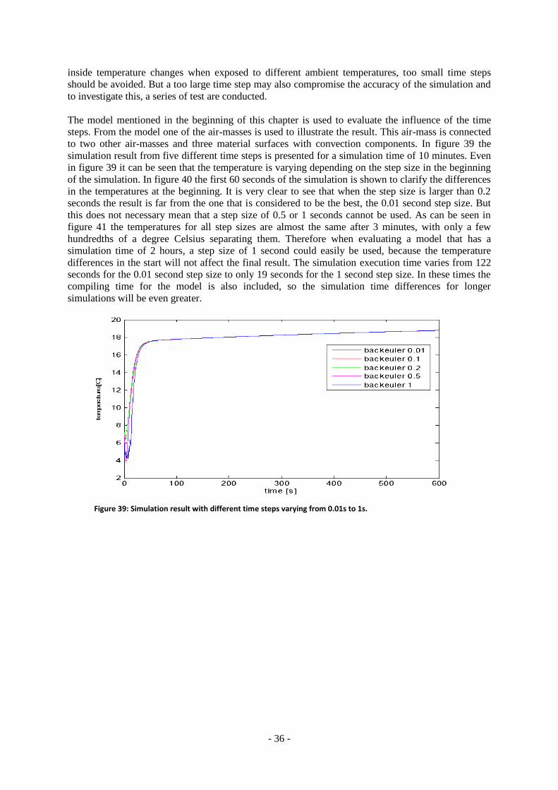
- 36 -
inside temperature changes when exposed to different ambient temperatures, too small time steps
should be avoided. But a too large time step may also compromise the accuracy of the simulation and
to investigate this, a series of test are conducted.
The model mentioned in the beginning of this chapter is used to evaluate the influence of the time
steps. From the model one of the air-masses is used to illustrate the result. This air-mass is connected
to two other air-masses and three material surfaces with convection components. In figure 39 the
simulation result from five different time steps is presented for a simulation time of 10 minutes. Even
in figure 39 it can be seen that the temperature is varying depending on the step size in the beginning
of the simulation. In figure 40 the first 60 seconds of the simulation is shown to clarify the differences
in the temperatures at the beginning. It is very clear to see that when the step size is larger than 0.2
seconds the result is far from the one that is considered to be the best, the 0.01 second step size. But
this does not necessary mean that a step size of 0.5 or 1 seconds cannot be used. As can be seen in
figure 41 the temperatures for all step sizes are almost the same after 3 minutes, with only a few
hundredths of a degree Celsius separating them. Therefore when evaluating a model that has a
simulation time of 2 hours, a step size of 1 second could easily be used, because the temperature
differences in the start will not affect the final result. The simulation execution time varies from 122
seconds for the 0.01 second step size to only 19 seconds for the 1 second step size. In these times the
compiling time for the model is also included, so the simulation time differences for longer
simulations will be even greater.
Figure 39: Simulation result with different time steps varying from 0.01s to 1s.
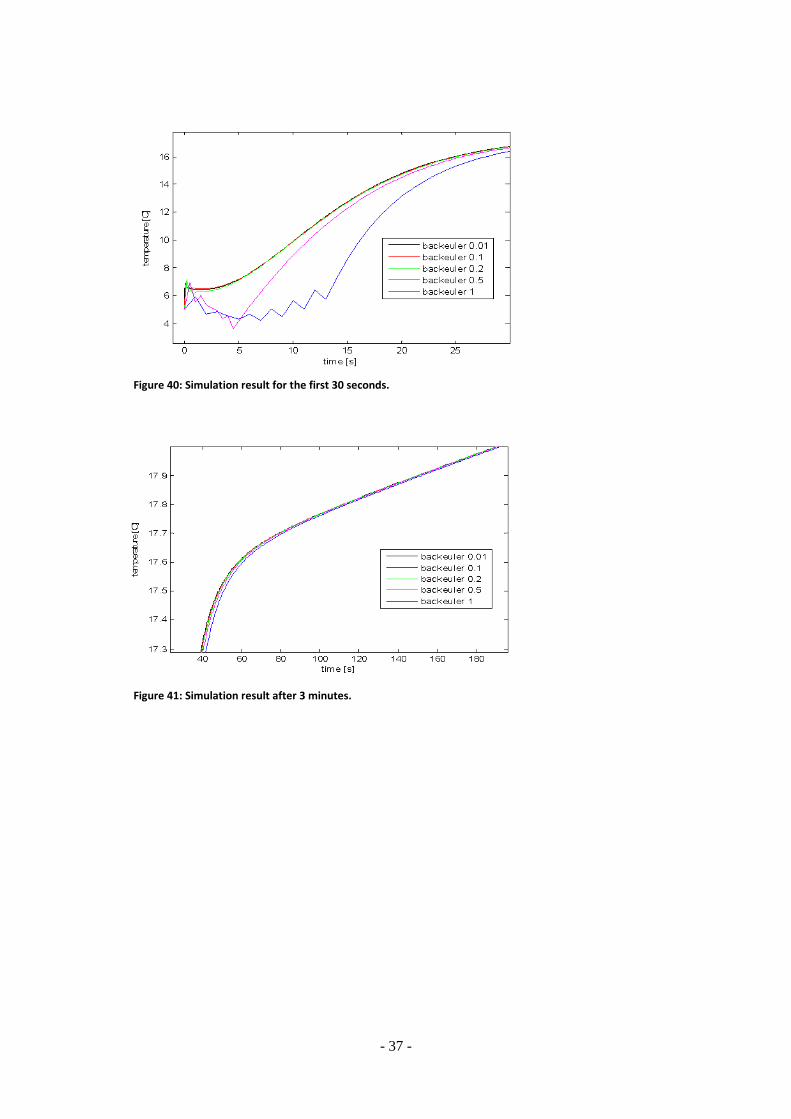
- 37 -
Figure 40: Simulation result for the first 30 seconds.
Figure 41: Simulation result after 3 minutes.
- 38 -
4. The Car Compartment Temperature Model in Simscape
In this chapter it is described how a physical temperature model of a car cabin is constructed in
Simscape using the experience from chapter 2 and 3.
4.1. Measurement Data
The model described in this chapter has to be validated and for this measurement data is used.
Measurements has for other purposes already been performed before the work with building a
physical model started. Meaning that sufficient measurements for validating the model are available
and there is no need to perform new measurements within this work.
The available measurements have been performed in a climate wind tunnel where the ambient
temperature is set to be constant. The car is driven, on rollers, according to a specified speed profile.
In order to represent the wind that would occur outside due to vehicle speed, the climate wind tunnel
gives a wind speed following the vehicle speed.
4.2. Simplifications and Assumptions
To simplify the construction of the Simscape model and to minimize computation time only half the
car is considered. Splitting the cabin in two and only using the left side can be done since the car is
symmetric. Doing this means that the effect of different temperature settings on the front left and right
seats cannot be evaluated. However this effect will not be different from the temperature analysis that
is done from the floor and up and from the front of the cabin to the back.
A larger simplification that is done in the model is that only one dimensional heat transfer is
considered. For the window surfaces this is true since the thickness is much less than the surface area,
but for other surfaces such as the doors this is not true since the thickness is 1/5 of the width. However
if the hole side of the car is considered the thickness can be regarded as being much less than the
surface area.
As mentioned in chapter 2.1 conduction the effect of radiation can be added to the convection. So
instead of having two different heat transfer coefficients and two different components in Simscape,
only one combined heat transfer coefficient is needed.
The effect of radiation from the sun is neglected in this model because the measurement data used to
compare the model against is recorded without the influence of sunshine.
On the outside of the car only one heat transfer coefficient is used to describe the convection from the
outer surfaces to the ambient air. Wind speed on the outer surfaces will vary depending on the shape
of the car and there will also be variations due to laminar or turbulent flow. The simplification will
give that some parts of the car might lose more energy than others, and some less, but the total energy
loss will be close to the case where all surfaces have different heat transfer coefficients.
Beside the simplifications mentioned above, it is assumed in the model that:
The angle of the air inlets are fixed in one position
There are no leakage from the compartment, between inlet and outlet
Only laminar flow is considered

- 39 -
4.3. What the Model Includes
The base for the model created in Simscape in this chapter is a car with 4 side doors. To get realistic
values of the air volumes, material volumes and surface areas the inside of the car is measured. All
larger surfaces are measured but smaller surfaces such as the steering wheel, gearstick and contacts
are not measured but their area estimated and added to the surfaces where they are mounted.
All the ventilation nozzles in the car are located and their location noted so that they can be placed
correctly in the model. All the nozzles are listed in table 6. The same is done with all material surfaces
and volumes so that they also can be placed correctly in relation to each other and the materials used
in model are listed in table 7.
Since the model is to be compared to measurements that are done in a lab where there is no driver or
passenger present in the car, there is no need to create a model of these. Another thing that is not
included in the model is the measurement equipment that is used in the lab to record the temperatures.
This equipment will dissipate heat but it is considered to very a small amount compared to the warm
or cold air that is entering the cabin through the nozzles.
Also the volume of the air is measured and divided into zones so that each of them will affect, or be
affected by, their neighboring material surfaces. How the air is divided can be seen in chapter 4.4,
Constructing the Model.
Table 6: Defrosters and ventilations which are implemented in the model.
Ventilation ducts
Defroster center (front window)
Defroster left (side window)
Ventilation center (driver)
Ventilation left (driver)
Ventilation front left foot (driver)
Ventilation rear left foot (passenger)
Table 7: Materials which are implemented in the model front and rear.
Front Rear
Front window Rear window
Front side window Rear side window
Roof Roof
Floor Floor
Door Door
Front seat Rear seat
Center stack
Dash
4.4. Constructing the Model
The model is constructed using all techniques described in chapter 3, modeling in Simscape. The
starting point for the model structure is the division of the air into smaller volumes that in some way
can be separated by the interior of the cabin. Inspired by [19] the air in both the front and rear of the
cabin is split up into three separate vertical air zones. The lower of these zones is called the “foot
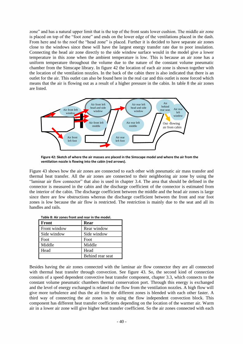
- 40 -
zone” and has a natural upper limit that is the top of the front seats lower cushion. The middle air zone
is placed on top of the “foot zone” and ends on the lower edge of the ventilations placed in the dash.
From here and to the roof the “head zone” is placed. Further it is decided to have separate air zones
close to the windows since these will have the largest energy transfer rate due to poor insulation.
Connecting the head air zone directly to the side window surface would in the model give a lower
temperature in this zone when the ambient temperature is low. This is because an air zone has a
uniform temperature throughout the volume due to the nature of the constant volume pneumatic
chamber from the Simscape library. In figure 42 the location of each air zone is shown together with
the location of the ventilation nozzles. In the back of the cabin there is also indicated that there is an
outlet for the air. This outlet can also be found here in the real car and this outlet is none forced which
means that the air is flowing out as a result of a higher pressure in the cabin. In table 8 the air zones
are listed.
Figure 43 shows how the air zones are connected to each other with pneumatic air mass transfer and
thermal heat transfer. All the air zones are connected to their neighboring air zone by using the
“laminar air flow connector” that also is used in chapter 3.4. The area that should be defined in the
connector is measured in the cabin and the discharge coefficient of the connector is estimated from
the interior of the cabin. The discharge coefficient between the middle and the head air zones is large
since there are few obstructions whereas the discharge coefficient between the front and rear foot
zones is low because the air flow is restricted. The restriction is mainly due to the seat and all its
handles and rails.
Table 8: Air zones front and rear in the model.
Front Rear
Front window Rear window
Side window Side window
Foot Foot
Middle Middle
Head Head
Behind rear seat
Besides having the air zones connected with the laminar air flow connector they are all connected
with thermal heat transfer through convection. See figure 43. So, the second kind of connection
consists of a speed dependent convective heat transfer component, chapter 3.3, which connects to the
constant volume pneumatic chambers thermal conservation port. Through this energy is exchanged
and the level of energy exchanged is related to the flow from the ventilation nozzles. A high flow will
give more turbulence and thus the air from the different zones is blended with each other faster. A
third way of connecting the air zones is by using the flow independent convection block. This
component has different heat transfer coefficients depending on the location of the warmer air. Warm
air in a lower air zone will give higher heat transfer coefficient. So the air zones connected with each
Air front
left foot
Air front left
middle
Air front left
head and side
window Air front left
window
Air rear left
head and side
window
Air rear left
middle
Air rear
left foot
Air rear
left
window
Out -flowing
air from cabin
Air
behind
rear seat.
Figure 42: Sketch of where the air masses are placed in the Simscape model and where the air from the ventilation nozzle is flowing into the cabin (red arrows).
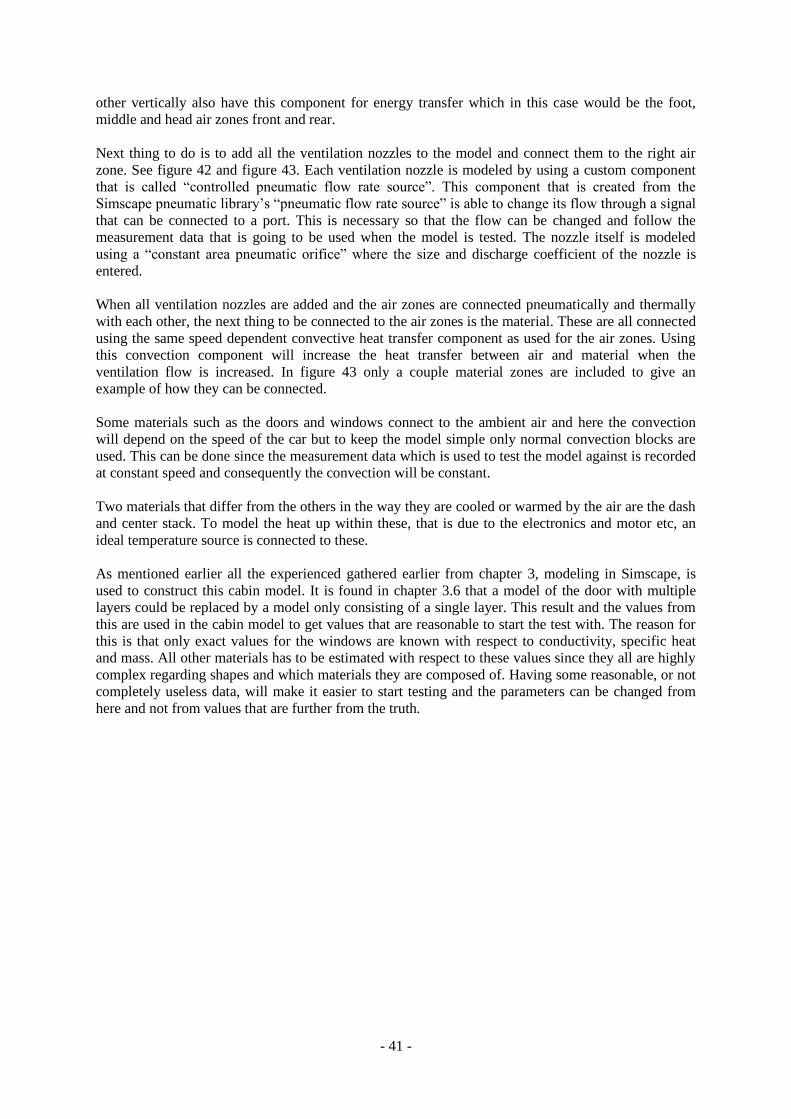
- 41 -
other vertically also have this component for energy transfer which in this case would be the foot,
middle and head air zones front and rear.
Next thing to do is to add all the ventilation nozzles to the model and connect them to the right air
zone. See figure 42 and figure 43. Each ventilation nozzle is modeled by using a custom component
that is called “controlled pneumatic flow rate source”. This component that is created from the
Simscape pneumatic library’s “pneumatic flow rate source” is able to change its flow through a signal
that can be connected to a port. This is necessary so that the flow can be changed and follow the
measurement data that is going to be used when the model is tested. The nozzle itself is modeled
using a “constant area pneumatic orifice” where the size and discharge coefficient of the nozzle is
entered.
When all ventilation nozzles are added and the air zones are connected pneumatically and thermally
with each other, the next thing to be connected to the air zones is the material. These are all connected
using the same speed dependent convective heat transfer component as used for the air zones. Using
this convection component will increase the heat transfer between air and material when the
ventilation flow is increased. In figure 43 only a couple material zones are included to give an
example of how they can be connected.
Some materials such as the doors and windows connect to the ambient air and here the convection
will depend on the speed of the car but to keep the model simple only normal convection blocks are
used. This can be done since the measurement data which is used to test the model against is recorded
at constant speed and consequently the convection will be constant.
Two materials that differ from the others in the way they are cooled or warmed by the air are the dash
and center stack. To model the heat up within these, that is due to the electronics and motor etc, an
ideal temperature source is connected to these.
As mentioned earlier all the experienced gathered earlier from chapter 3, modeling in Simscape, is
used to construct this cabin model. It is found in chapter 3.6 that a model of the door with multiple
layers could be replaced by a model only consisting of a single layer. This result and the values from
this are used in the cabin model to get values that are reasonable to start the test with. The reason for
this is that only exact values for the windows are known with respect to conductivity, specific heat
and mass. All other materials has to be estimated with respect to these values since they all are highly
complex regarding shapes and which materials they are composed of. Having some reasonable, or not
completely useless data, will make it easier to start testing and the parameters can be changed from
here and not from values that are further from the truth.
- 42 -
Air front
left head
and side
window
Air rear
left head
and side
window
Air behind
rear seat.
Air front
left middleAir rear left
middle
Air front
left footAir rear left
foot
Air front
left
window
Air rear
left
window
Air zone
Air inlet or outlet
Laminar air flow connector
Flow dependent convection between air zones
Flow independent convection between air zones
Convection between air and material
Conduction through a material
Material
Figure 43: The main idea of how the air and material zones are connected with pneumatic laminar air flow connectors and convective heat transfer. Air inlets/outlets and conduction through the materials are also included.
- 43 -
4.5. Adjusting Parameters to fit Measurement Data
Now that the model is created in Simscape, and all necessary physical material and air constants
defined in separate m-files in MATLAB, the last task is to adjust convection, conduction, specific
heat and also mass where these are estimated. The important temperature in the tuning of the model is
considered to be the temperature at the driver’s head. All other temperatures will not be totally
neglected but only adjusted if these seem unrealistic. The measurement data that is used for the
adjusting of the parameters are from a test where the ambient temperature is -20deg Celsius and the
speed of the car and the wind speed is constant at 100 km/h. In the result chapter, 6, the model will be
tested against another measurement data set where the ambient temperature is warmer.
Since there are many heat transfer coefficients between air and air and air and material it would be too
work intensive to adjust these individually. Instead a common value for all convection between
material and air is used. Another common constant is used for convection between air zones. This
assumption might not be right since the shape and surface of the materials are very different. But
since the material data that are used, except from the windows, is approximated an exact convection
constant is difficult to determine and therefore an approximation might be just as good in this case.
The common convection constants described above are for natural convection. To adjust the forced
convection inside the cabin, the effect from the ventilation nozzles when air flow is varying, two
common constants are needed. The first is a constant that increases the flow dependent convection
between air and material while the next controls the flow dependent convection between air zones.
Besides the flow dependent constants a constant is needed that controls the flow independent
convection between the air zones that are placed on top of each other. This is because the heat transfer
coefficients are different depending on if the warmer air zone is on top or not. The last common
constant that is used is the one that controls the heat convection from the outer surfaces of the car
model to the ambient air.
In the following text a short description of the steps taken to calibrate the model to fit the
measurement data is presented. Not all steps are included but a few of the most important are included
together with a figure to illustrate the problem. The measurement data used contain more than two and
a half hours of data, so the objective will be to fit the model to the steady state temperature initially
and later try and get the transients right.
To have some values that are realistic as a starting point data from tables in [1] are used. The heat
transfer coefficient value for natural convection is stated here to be between 2 and 25 , and
for forced convection the value is between 25 and 250 . For the convection on the inside of
the car model a low natural convection is chosen, in this case 5 . For the outside convection
between material and ambient, a higher heat transfer coefficient is chosen since this is forced
convection. To begin with this value is chosen to be 50 . Figure 44 shows the result from the
first simulation. From the plot there are four obvious errors with the Simscape model and its
parameters. First it is clear that the steady state temperature is too low. After about 5000 seconds the
error in temperature is approximately 9 degrees Celsius. One of the reasons for this temperature
difference could be that the convection heat transfer coefficient between the ambient air and the outer
surface of the cabin model is too high and thus too much energy is dissipated away from the cabin.
Another reason could be that the conductivity of the material is too high and thus too much energy is
conducted through the material. However decreasing the conductivity would also have a negative
effect on the second problem of the simulation result which is the slightly higher temperature in the
beginning (1000-4000 seconds) compared to the steady state temperature after 5000 seconds.
Decreasing the conductivity would decrease the energy transfer by convection from air to material.
This is because less energy is transported through the material and therefore the temperature on the
inside of the material is higher thus the convective heat transfer would be less due to reduced
temperature difference. In chapter 2.1 these heat transfer characteristics are described. Using the
example from chapter 2.1 the heat transfer rate can be seen as a function of the total resistance from
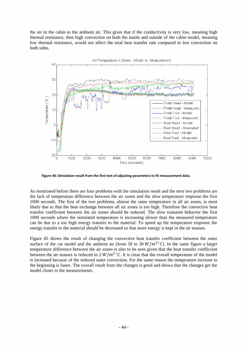
- 44 -
the air in the cabin to the ambient air. This gives that if the conductivity is very low, meaning high
thermal resistance, then high convection on both the inside and outside of the cabin model, meaning
low thermal resistance, would not affect the total heat transfer rate compared to low convection on
both sides.
Figure 44: Simulation result from the first test of adjusting parameters to fit measurement data.
As mentioned before there are four problems with the simulation result and the next two problems are
the lack of temperature difference between the air zones and the slow temperature response the first
1000 seconds. The first of the two problems, almost the same temperature in all air zones, is most
likely due to that the heat exchange between all air zones is too high. Therefore the convective heat
transfer coefficient between the air zones should be reduced. The slow transient behavior the first
1000 seconds where the simulated temperature is increasing slower than the measured temperature
can be due to a too high energy transfer to the material. To speed up the temperature response the
energy transfer to the material should be decreased so that more energy is kept in the air masses.
Figure 45 shows the result of changing the convective heat transfer coefficient between the outer
surface of the car model and the ambient air (from 50 to 30 ). In the same figure a larger
temperature difference between the air zones is also to be seen given that the heat transfer coefficient
between the air masses is reduced to 2 . It is clear that the overall temperature of the model
is increased because of the reduced outer convection. For the same reason the temperature increase in
the beginning is faster. The overall result from the changes is good and shows that the changes get the
model closer to the measurements.
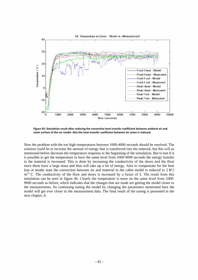
- 45 -
Figure 45: Simulation result after reducing the convective heat transfer coefficient between ambient air and outer surface of the car model. Also the heat transfer coefficient between air zones is reduced.
Now the problem with the too high temperatures between 1000-4000 seconds should be resolved. The
solution could be to increase the amount of energy that is transferred into the material, but this will as
mentioned before decrease the temperature response in the beginning of the simulation. But to test if it
is possible to get the temperature to have the same level from 1000-9000 seconds the energy transfer
to the material is increased. This is done by increasing the conductivity of the doors and the floor
since these have a large mass and thus will take up a lot of energy. Also to compensate for the heat
loss at steady state the convection between air and material in the cabin model is reduced to 2 . The conductivity of the floor and doors is increased by a factor of 5. The result from this
simulation can be seen in figure 46. Clearly the temperature is more on the same level from 1000-
9000 seconds as before, which indicates that the changes that are made are getting the model closer to
the measurements. So continuing tuning the model by changing the parameters mentioned here the
model will get ever closer to the measurement data. The final result of the tuning is presented in the
next chapter, 6.

- 46 -
Figure 46: Simulation result from changes in the floor and door conductivity together with a decrease off the convective heat transfer coefficient between air and material.
- 47 -
5. Advantages and Drawbacks with Physical Modeling in Simscape
There are both pros and cons with physical modeling and they will be discussed in this chapter, both
for physical modeling in general and specifically in Simscape. Among the advantages with physical
modeling in general is the intuitive way to construct the physical models, using components and
physical relationships. It is also easier to understand a model that someone else has constructed.
Even in a physical model simplifications are possible, but simplifying too much might give the
drawbacks that the model acquires non-physical properties or that it does not behave as desired.
Though, using material as an example that is a topic for this report, it should be considered that once
having a good enough material model, it is in large extent possible to use that experience to construct
new similar models. E.g. constructing a car door as showed in the door example, chapter 3.6 is an
experience that can be used when constructing other car doors.
The bullets below summarize advantages and drawbacks with physical modeling in general and in
Simscape.
Advantages:
It is intuitive to construct a physical model and easier to understand a model that someone else
created
It is easier to understand which parameters to modify when trying to fit a model to
measurement data
When all physical properties, e.g. air volumes and material properties, are in place and the
model is calibrated, it should be possible to apply the model to another car model, that is either
larger or smaller, since only the physical sizes of the air volumes and material are needed
While working with a Simscape model things are easier to overview if components or sub
models are created in blocks. Soon it is found that these sub model blocks are convenient to
reuse, only changing parameters if necessary. This could be taken one step further creating a
component library with sub model blocks, only having ports visible to the user. A user
interface could be used to change parameters. This is smooth for experienced users but also
users with only little experience of Simscape could take part of the component library and
construct their own models
Drawbacks:
To be able to use physical modeling for temperature models of several different car models, it
is necessary to create some kind of library including correct data regarding heat conductivity
and material properties
If the model is simplified too much it will make it more non-physical, which might remove the
point of making a physical model. See the door example in chapter 3.6
Simscape is still a young software, first released with MATLAB R2007a and the number of
libraries and components have been growing the last few years, but there are still things that
can be and probably will be better. One example is that busses for Simscape signals are still
missing in R2011a. This means that every single signal need its own connection and that gives
a large number of connections. With busses it would be possible to combine several signals
and make the model smoother
Remember that constructing a mathematical model also means a lot of work, particularly when
defining and setting parameters. The drawbacks with physical modeling and Simscape are possible to
overcome especially when looking at the advantages such as understanding the model and adapt it to
other car models.

- 48 -
6. Results
The model is tested using inputs, air mass flows and their temperatures, from measurements. Then the
compartment temperatures from the measurement are compared to the outputs from the model, i.e. the
model temperatures in different air zones, see chapter 4.4 and 4.5 for more information about how the
model is constructed and its parameters adjusted.
The final values that where found when adjusting the parameters were in some cases not according to
the table data from [1]. As mentioned in chapter 4.5 the natural convection heat transfer coefficient
will have values from 2 to 25 and the forced convection, values from 25 to 250 .
To get the model to match the measurement data as well as it is presented in figure 47 the natural
convection heat transfer coefficient between air and air and air and material is set to 1 and
the forced convection between the outer surface and the ambient air has a value of 12 . Both
the natural convection on the inside and the forced convection on the outside are too low compared to
the table data. This indicates, especially for the case of the low forced convection on the outside, that
the overall conductivity of the material is too high. So the material data needs to be evaluated to
obtain more realistic heat transfer coefficients for the convection. Either this has to be done through
experiments or by getting access to data from earlier experiments. However the low convection heat
transfer coefficient between the air and air can in this case be explained by the fact the pneumatic part
itself transfers heat, and thus lower heat transfer coefficients are needed.
Figure 47 shows the result comparing model and measurement for the front left head and the rear left
head air zones. The measurement is performed in cold climate at about – 20 , starting with a cold
car. It is a first order system, but it can seem like a slow response in the beginning for the reason that
the car engine and therefore the air blowing into the compartment is cold. It can be seen that after 25
minutes (1500 seconds) and in steady state, the model’s amplitude corresponds very well to the
amplitude of the measurement. In the start though, the model is a bit slower than the measurement.
See figure 49(a) for a zoom of the first 700 seconds.
Figure 47: Comparing model and measurement for front left head and rear left head.
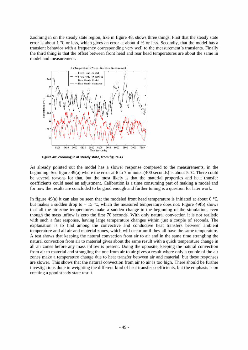
- 49 -
Zooming in on the steady state region, like in figure 48, shows three things. First that the steady state
error is about 1 or less, which gives an error at about 4 % or less. Secondly, that the model has a
transient behavior with a frequency corresponding very well to the measurement’s transients. Finally
the third thing is that the offset between front head and rear head temperatures are about the same in
model and measurement.
Figure 48: Zooming in at steady state, from figure 47
As already pointed out the model has a slower response compared to the measurements, in the
beginning. See figure 49(a) where the error at 6 to 7 minutes (400 seconds) is about 5 . There could
be several reasons for that, but the most likely is that the material properties and heat transfer
coefficients could need an adjustment. Calibration is a time consuming part of making a model and
for now the results are concluded to be good enough and further tuning is a question for later work.
In figure 49(a) it can also be seen that the modeled front head temperature is initiated at about 0 ,
but makes a sudden drop to – 15 , which the measured temperature does not. Figure 49(b) shows
that all the air zone temperatures make a sudden change in the beginning of the simulation, even
though the mass inflow is zero the first 70 seconds. With only natural convection it is not realistic
with such a fast response, having large temperature changes within just a couple of seconds. The
explanation is to find among the convective and conductive heat transfers between ambient
temperature and all air and material zones, which will occur until they all have the same temperature.
A test shows that keeping the natural convection from air to air and in the same time strangling the
natural convection from air to material gives about the same result with a quick temperature change in
all air zones before any mass inflow is present. Doing the opposite, keeping the natural convection
from air to material and strangling the one from air to air gives a result where only a couple of the air
zones make a temperature change due to heat transfer between air and material, but these responses
are slower. This shows that the natural convection from air to air is too high. There should be further
investigations done in weighting the different kind of heat transfer coefficients, but the emphasis is on
creating a good steady state result.
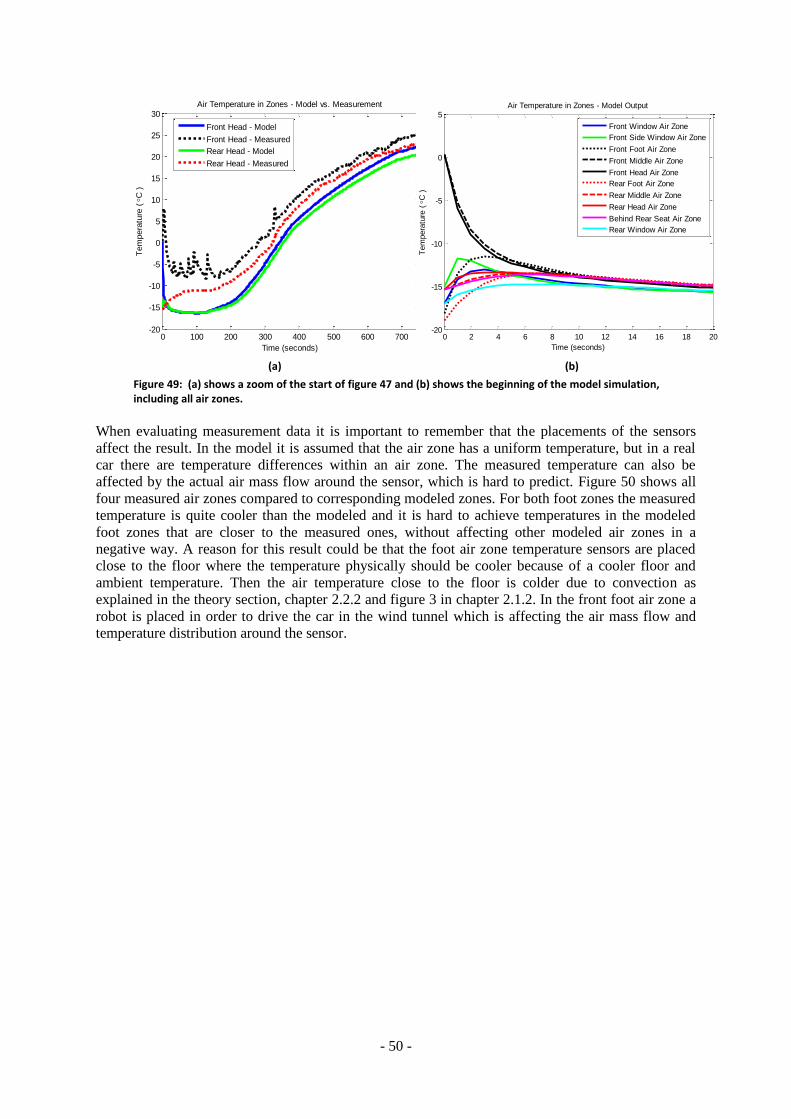
- 50 -
(a) (b)
Figure 49: (a) shows a zoom of the start of figure 47 and (b) shows the beginning of the model simulation, including all air zones.
When evaluating measurement data it is important to remember that the placements of the sensors
affect the result. In the model it is assumed that the air zone has a uniform temperature, but in a real
car there are temperature differences within an air zone. The measured temperature can also be
affected by the actual air mass flow around the sensor, which is hard to predict. Figure 50 shows all
four measured air zones compared to corresponding modeled zones. For both foot zones the measured
temperature is quite cooler than the modeled and it is hard to achieve temperatures in the modeled
foot zones that are closer to the measured ones, without affecting other modeled air zones in a
negative way. A reason for this result could be that the foot air zone temperature sensors are placed
close to the floor where the temperature physically should be cooler because of a cooler floor and
ambient temperature. Then the air temperature close to the floor is colder due to convection as
explained in the theory section, chapter 2.2.2 and figure 3 in chapter 2.1.2. In the front foot air zone a
robot is placed in order to drive the car in the wind tunnel which is affecting the air mass flow and
temperature distribution around the sensor.
0 100 200 300 400 500 600 700-20
-15
-10
-5
0
5
10
15
20
25
30Air Temperature in Zones - Model vs. Measurement
Time (seconds)
Tem
pera
ture
(
C )
Front Head - Model
Front Head - Measured
Rear Head - Model
Rear Head - Measured
0 2 4 6 8 10 12 14 16 18 20-20
-15
-10
-5
0
5Air Temperature in Zones - Model Output
Time (seconds)
Tem
pera
ture
(
C )
Front Window Air Zone
Front Side Window Air Zone
Front Foot Air Zone
Front Middle Air Zone
Front Head Air Zone
Rear Foot Air Zone
Rear Middle Air Zone
Rear Head Air Zone
Behind Rear Seat Air Zone
Rear Window Air Zone
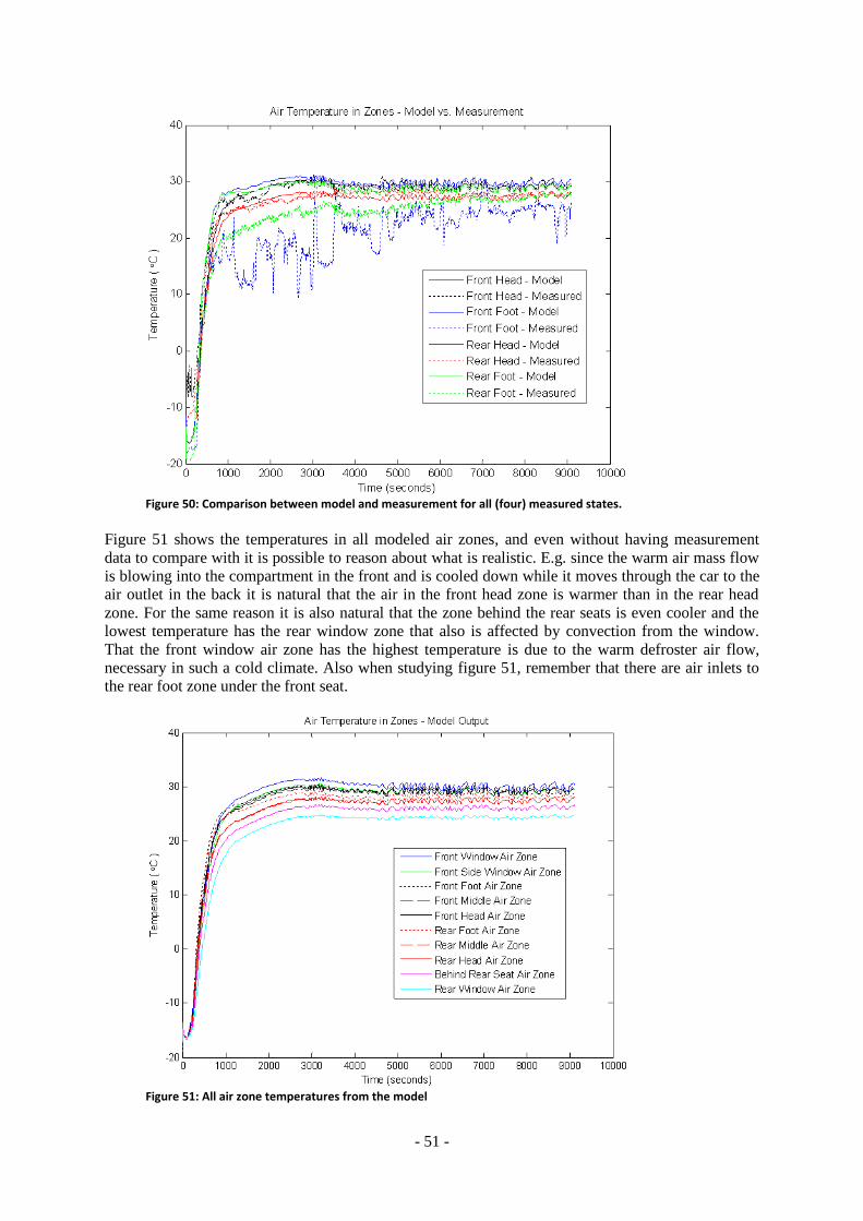
- 51 -
Figure 50: Comparison between model and measurement for all (four) measured states.
Figure 51 shows the temperatures in all modeled air zones, and even without having measurement
data to compare with it is possible to reason about what is realistic. E.g. since the warm air mass flow
is blowing into the compartment in the front and is cooled down while it moves through the car to the
air outlet in the back it is natural that the air in the front head zone is warmer than in the rear head
zone. For the same reason it is also natural that the zone behind the rear seats is even cooler and the
lowest temperature has the rear window zone that also is affected by convection from the window.
That the front window air zone has the highest temperature is due to the warm defroster air flow,
necessary in such a cold climate. Also when studying figure 51, remember that there are air inlets to
the rear foot zone under the front seat.
Figure 51: All air zone temperatures from the model
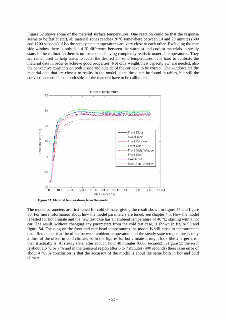
- 52 -
Figure 52 shows some of the material surface temperatures. One reaction could be that the response
seems to be fast at start, all material zones reaches 20 somewhere between 10 and 20 minutes (600
and 1200 seconds). Also the steady state temperatures are very close to each other. Excluding the rear
side window there is only 3 – 4 difference between the warmest and coolest materials in steady
state. In the calibration there is no focus on achieving completely realistic material temperatures. They
are rather used as help states to reach the desired air zone temperatures. It is hard to calibrate the
material data in order to achieve good properties. Not only weight, heat capacity etc. are needed, also
the convective constants on both inside and outside of the car have to be correct. The windows are the
material data that are closest to reality in the model, since these can be found in tables, but still the
convection constants on both sides of the material have to be calibrated.
Figure 52: Material temperatures from the model.
The model parameters are first tuned for cold climate, giving the result shown in figure 47 and figure
50. For more information about how the model parameters are tuned, see chapter 4.5. Now the model
is tested for hot climate and the new test case has an ambient temperature of 40 , starting with a hot
car. The result, without changing any parameters from the cold test case, is shown in figure 53 and
figure 54. Focusing on the front and rear head temperatures the model is still close to measurement
data. Remember that the offset between ambient temperature and the steady state temperature is only
a third of the offset in cold climate, so in the figures for hot climate it might look like a larger error
than it actually is. At steady state, after about 1 hour 40 minutes (6000 seconds) in figure 53 the error
is about 1.5 or 7 % and in the transient region after 6 to 7 minutes (400 seconds) there is an error of
about 4 . A conclusion is that the accuracy of the model is about the same both in hot and cold
climate.

- 53 -
Figure 53: Model output for front and rear head air zones compared to measurement for a test in hot climate, with an ambient temperature of 40
Figure 54: Model output for head and foot air zones, front and rear, compared to measurement for a test in hot climate, with an ambient temperature of 40
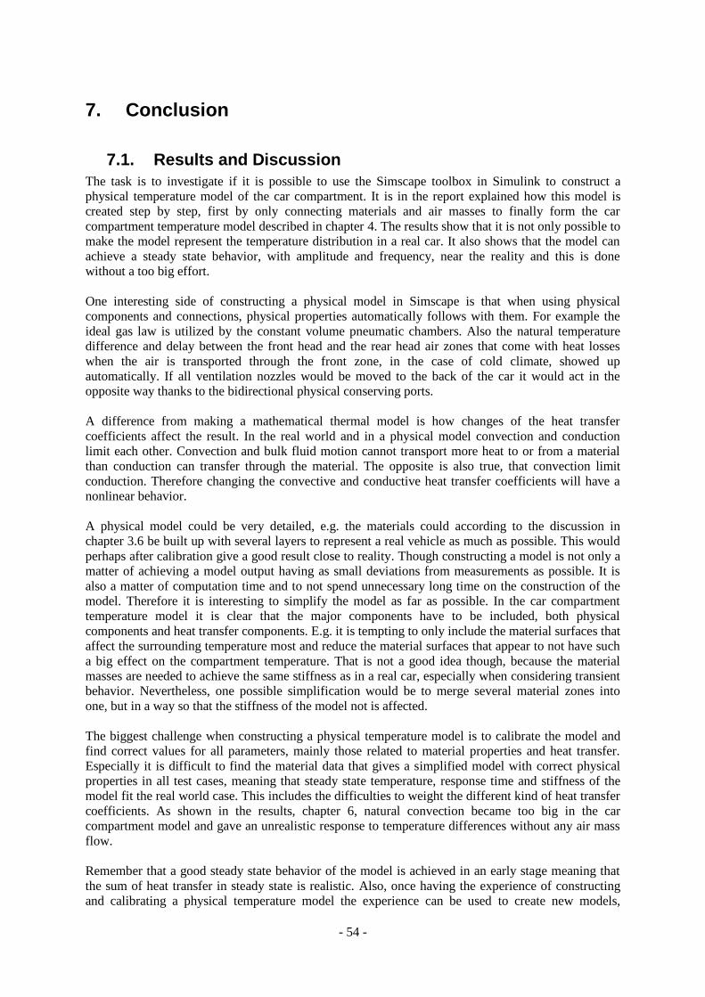
- 54 -
7. Conclusion
7.1. Results and Discussion
The task is to investigate if it is possible to use the Simscape toolbox in Simulink to construct a
physical temperature model of the car compartment. It is in the report explained how this model is
created step by step, first by only connecting materials and air masses to finally form the car
compartment temperature model described in chapter 4. The results show that it is not only possible to
make the model represent the temperature distribution in a real car. It also shows that the model can
achieve a steady state behavior, with amplitude and frequency, near the reality and this is done
without a too big effort.
One interesting side of constructing a physical model in Simscape is that when using physical
components and connections, physical properties automatically follows with them. For example the
ideal gas law is utilized by the constant volume pneumatic chambers. Also the natural temperature
difference and delay between the front head and the rear head air zones that come with heat losses
when the air is transported through the front zone, in the case of cold climate, showed up
automatically. If all ventilation nozzles would be moved to the back of the car it would act in the
opposite way thanks to the bidirectional physical conserving ports.
A difference from making a mathematical thermal model is how changes of the heat transfer
coefficients affect the result. In the real world and in a physical model convection and conduction
limit each other. Convection and bulk fluid motion cannot transport more heat to or from a material
than conduction can transfer through the material. The opposite is also true, that convection limit
conduction. Therefore changing the convective and conductive heat transfer coefficients will have a
nonlinear behavior.
A physical model could be very detailed, e.g. the materials could according to the discussion in
chapter 3.6 be built up with several layers to represent a real vehicle as much as possible. This would
perhaps after calibration give a good result close to reality. Though constructing a model is not only a
matter of achieving a model output having as small deviations from measurements as possible. It is
also a matter of computation time and to not spend unnecessary long time on the construction of the
model. Therefore it is interesting to simplify the model as far as possible. In the car compartment
temperature model it is clear that the major components have to be included, both physical
components and heat transfer components. E.g. it is tempting to only include the material surfaces that
affect the surrounding temperature most and reduce the material surfaces that appear to not have such
a big effect on the compartment temperature. That is not a good idea though, because the material
masses are needed to achieve the same stiffness as in a real car, especially when considering transient
behavior. Nevertheless, one possible simplification would be to merge several material zones into
one, but in a way so that the stiffness of the model not is affected.
The biggest challenge when constructing a physical temperature model is to calibrate the model and
find correct values for all parameters, mainly those related to material properties and heat transfer.
Especially it is difficult to find the material data that gives a simplified model with correct physical
properties in all test cases, meaning that steady state temperature, response time and stiffness of the
model fit the real world case. This includes the difficulties to weight the different kind of heat transfer
coefficients. As shown in the results, chapter 6, natural convection became too big in the car
compartment model and gave an unrealistic response to temperature differences without any air mass
flow.
Remember that a good steady state behavior of the model is achieved in an early stage meaning that
the sum of heat transfer in steady state is realistic. Also, once having the experience of constructing
and calibrating a physical temperature model the experience can be used to create new models,
- 55 -
reaching a desired transient behavior. E.g. methods can be established to find the most important
material data and skills are developed in how to figure out the heat transfer coefficients.
7.2. Future Work
As mentioned before a big problem when creating the model is to get good data regarding the
properties of the materials. In the model only the windows have the right properties and all other
materials have approximated values. These approximations are again taken from the result in chapter
3.6 where it is shown, that a door model consisting of several material layers, can be approximated
with a single layer of material. The result is based on a very simple model so the values used could be
far from real values. That a satisfying result is obtained anyway can be due to that the convection
constants in the model are adjusted so that the simulated temperatures would follow the
measurements. A lower convection constant on the inside of the cabin would compensate for a
conduction constant that is estimated with a too high value. If Simscape is to be used for future
models it would be important to have some real data from measurements that contain better values
concerning conductivity, mass, specific heat and also convection. Another way to get better estimates
on the material properties would be to construct more exact models of the components in the cabin,
like doors, roof and seats. These models could be constructed from the data that is accessible from the
3D drawings of the cars, where all data for the materials are included. It would be an extensive work
but the models could be reused for new car models and thus be less time consuming when creating
new Simscape models.
It is discovered that the standard Simscape libraries do not hold sufficient components for the
temperature model to be constructed, so new components have to be created. These components are
not difficult to create but if several persons are working with different models and all creating own
components it will not be possible for others to use these models without the new component libraries.
So to avoid problems using different models, a structure for how to handle custom component
libraries within the companies should be implemented.
Despite the problems described above it would be interesting to see how the model would work if the
material data is changed, with respect to area, to fit a smaller or a larger car. It would also be
interesting to see if the model, that is optimized using measurements from cold climate, would work
well when measurements from warm climate is used. Not just for the one tested here but also for one
where radiation from the sun affects the temperature..
Creating more complex models that give more realistic results will increase computations and thus
increase the simulation time. If these get too long some simplification may be needed in the model. It
could be investigated if some of the materials connected to the same air zone could be compiled into
one single material and through this make the model simpler. Another way to simplify the model
could be to remove some air zones, it may not be optimal to have three vertical air zones - it might be
sufficient with two. Also it might not be necessary with the extra air zone that is added to work as
buffer between the windows and the other air zones.

- 56 -
8. References
[1] Çengel, Yunus A.: Heat and Mass Transfer: a pratical approach, 3rd
edition, McGraw-
Hill, New York 2007.
[2] Holman J.P.: Heat Transfer, 9th edition, McGraw Hill, New York 2002.
[3] Çengel, Yunus A.: Heat transfer: a practical approach, McGraw-Hill, Boston 2003.
[4] Incropera, Frank P. et al: Fundamentals of heat and mass transfer, 6th edition, John
Wiley & Sons, New York, 2007.
[5] Çengel, Yunus A, Turner, Robert H. and Cimbala, John M.: Fundamentals of thermal-
fluid science, 3rd
edition, Mc Graw Hill, New York 2008.
[6] http://www.mathworks.se/products/simscape/, access date 2011-10-31
[7] http://www.mathworks.se/help/toolbox/physmod/simscape/rn/bq2j20j-1_1.html, access
date 2011-10-31
[8] http://www.3ds.com/products/catia/portfolio/dymola/overview/, access date 2011-10-31
[9] http://www.mathworks.se/help/toolbox/physmod/simscape/gs/bp5oe5y-1.html, access
date 2011-10-31
[10] http://en.wikipedia.org/w/index.php?title=Dymola&oldid=453426407, access date 2011-
10-31
[11] http://www.mathworks.se/help/toolbox/physmod/simscape/ug/bq89sba-1.html, access
date 2011-10-31
[12] http://www.mathworks.se/help/toolbox/physmod/simscape/lang/brmrvp3-1.html, access
date 2011-11-02
[13] http://www.mathworks.se/help/toolbox/physmod/simscape/lang/brs66zm.html, access
date 2011-11-03
[14] http://www.mathworks.se/help/toolbox/physmod/simscape/ug/bq_hwn6-1.html, access
date 2011-11-02
[15] http://www.mathworks.se/help/toolbox/physmod/simscape/lang/brn4h9l-1.html, access
date 2011-11-10.
[16] http://www.mathworks.se/help/releases/R2011a/toolbox/simulink/ug/f11-
69449.html#bsdkv37, access date 2011-10-24.
[17] http://www.mathworks.se/help/toolbox/physmod/powersys/ref/currentvoltagesimscapeint
erfacegnd.html , access date 2011-10-24.
[18] http://www.mathworks.se/help/releases/R2011a/toolbox/physmod/simscape/ug/bsigllk.ht
ml#bsjplhe-1, access date 2011-10-25.
- 57 -
[19] Takuya Kubota, Ryo Watanabe and Hidenori Miyashita: Effects of Thermal Radiation
and Insolation on Passenger Compartments of an Automobile, 2010 IEEE International
Conference on Control Applications, Yokohama, Japan, 2010
[20] http://www.mathworks.se/help/releases/R2011a/toolbox/simulink/ug/f7-
8243.html#bridiag-7 , access date 2011-10-25.
[21] Aze-eddine Naamane, Mohammed Radouani and Abdelmjid Saka: Modeling of aircraft
braking system: Component oriented approach, International Journal of Research and
Reviews in Mechatronic Design and Simulation (IJRRMDS) Vol. 1, No. 3, Science
Academy Publisher, United Kingdom, 2011
Top Related