


Languages
Pages
Legal


LA-7708TThesis
UC-80Issued: March 1979
Thermal-Hydraulic Analysis Techniques
for Axisymmetric PebbJIe Bed
Nuclear Reactor Cores
Kenneth R. Stroh
- NOTICE-Thja report was prepared as an account of woiksponsored by the United Stales Government. Neither theUnited State* nor the United States Department ofEnergy, nor any of theli employees, not any of theircontractors, subcontractor!, or their employees, makesany watraniy, express 01 implied, or assumes any legalliability or responsibility for the accuracy, compler-neiiw usefulness of any information, apparatus, product 01process disclosed, or represents that its use would notinfringe privately owned rights.

TABLE OF CONTENTS
Chapter Page
List of Figures vi
Abstract U
I. INTRODUCTION 1
A. Pebble Bed Nuclear Reactor Concept 1B. Motivation of the Study 3
II. REVIEW OF THE LITERATURE 6
A. Introduction ..... 6B. Packed Bed Fluid Flow and Pressure Drop. .... 6C. Packed Bed Heat Transfer 11
III. MATHEMATICAL MODEL 14
A. Hydraulic Model 14
B. Thermal Model 20
IV. COMPUTER CODE PEBBLE 29
A. Solution Technique 29V. ORNL PBRE ANALYSIS 32
A. Pebble Bed Reactor Experiment 32B. Code Validation Concerns 34C. Void Fraction Distribution in the PBRE 37D. Comparison of Predictions with
Measured Values 40
E. Discussion of PBRE Results 48
VI. COUPLED THERMAL-HYDRAULIC TEST PROBLEM 54
A. KFA Power Reactor Design 54B. Numerical Model 54C. Boundary Conditions 56D. Lessons Learned in Debugging the Problem .... 59E. Discussion of Results 62
iv

TABLE OF CONTENTS (continued)Chapter Page
VII. CONCLUSIONS 80
ACKNOWLEDGMENTS 82
LIST OF REFERENCES 83
APPENDIX A. Numerical Solution Technique '. . . . 37
A.I The Doman of Integration 87A.2 Integration of the Equation 87A.3 The Successive-Substitution Formula 97
APPENDIX 8. Listing of Program PEBBLE andits Subroutines 101
APPENDIX C. Print Output for Analysis of KFA DesignCase 1013 143
APPENDIX D. Pr in t Output for Analysis of ORNL PBREBed 13FCa 161

LIST OF FIGURES
Page
A section view of a large power reactor design showingthe graphite reflector structure, the pebble bed corewith free surface, and the ball discharge structures. . . 2
2 Fuel-moderator element types proposed for pebble bednuclear reactors 4
3 Comparison of the Ergun equation with data fromsphere bed flow experiments ..... 12
4 Comparison of the new flow model with other modelsand experimental data . 16
5 Distribution of pebble thermal conductivitycorresponding to an idealized OTTO fuel cycle 28
6 The basic geometry of the ORNL PBRE is shownat the left. The letters E, I, FT and FC denotethe location of the exit faces above which measure-ments were made. The corresponding finite differencegrid is shown at the right. . 33
7 The radial distribution of <P for plugflow 36
8 Void fraction distribution used in PEBBLE to modelthe cylindrical portion of PBRE Bed 13 39
9 Calculated mass flux streamlines and isobars forPBRE Bed 13FCa 41
10 Calculated distribution of normalized velocityfor PBRE Bed 13FCa 42
11 Comparison of predicted and measured exit velocityprofiles above PBRE Bed 13Ea (entrance region) 44
12 Comparison of predicted and measured exit velocityprofiles above PBRE Bed 131a (lower half of bed) 45
13 Comparison of predicted and measured exit velocityprofiles above PBRE Bed 13FTa (flat-top bed, fillcone removed) „ 46
14 Comparison of predicted and measured exit velocityprofiles above PBRE Bed 13FCa (entire bed toppedby fill cone) 47
vi

LIST OF FIGURES (continued)Page
Comparison of predicted and measured exit velocityprofiles above PBRE Bed 13E for two different inlatReynolds numbers 49
16 Comparison of predicted and measured exit velocityprofiles above PBRE Bed 131 for two different inletReynolds numbers 50
17 Comparison of predicted and measured exit velocityprofiles above PBRE Bed 13FT for two differentinlet Reynolds numbers 51
18 Comparison of predicted and measured exit velocityprofiles above PBRE Bed 13FC for two differentinlet Reynolds numbers 52
19 A comparison of the physical reactor and the axi-symmetric model used in the analysis 55
20 Original grid used by PEBBLE, where radial gridlines 4-21 (of 22 total) correspond to those locationswhere VSOP supplies power per ball values for KFADesign Case 1013 57
21 Finite difference grid used for the thermal-hydraulic calculations ,. 58
22 Design for the core bottom structure showingthe complicated gas exit path 60
23 Distribution of thermal power per ball for KFAPR3000 Design Case 1013 63
24 Calculated distribution of the dimensionlessmass flux, G* 64
25 Calculated distribution of the coolant bulktemperature for KFA PR3000 Design Case 1013 65
26 Calculated distribution of the pebble averagesurface temperature for KFA PR3000 Design Case 1013. .. 66
27 Calculated distribution of the maximum internalfueled matrix temperature for KFA PR3000Design Case 1013 67
28 Calculated axial distribution of temperatures atthe core centerline for KFA PR3000 Design Case 1013. . . 68
vii

LIST OF FIGURES (continued)Page
Calculated axial distribution of temperatures atthe hot radius for KFA PR3OOO Design Case 1013 69
30 Calculated axial distribution of temperatures atthe cold radius for KFA PR3000 Design Case 1013 70
31 Calculated coolant outlet temperatures for KFAPR3000 Design Case 1013 , . . . 71
32 Contour plot of thermal power per ball values
from VSOP 72
33 Calculated mass flux streamlines. . . . . . . . 73
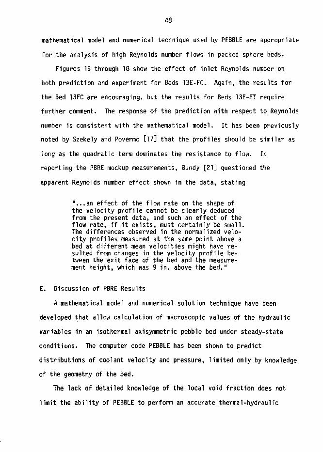
34 Calculated equipressure lines .... 74
35 Contour plot of calculated coolant bulk tenderer .u>-es. . . 7536 Contour plot of calculated pebble average vjrface
temperatures 76
37 Contour plot of calculated maxirmn irVTial fueledmatrix temperatures 77
38 Illustration of a portion of the finite difference gridshowing the area of integration for the differentialequations 88
viii

ABSTRACT OF THESIS
THERMAL-HYDRAULIC ANALYSIS TECHNIQUES FOR
AXISYMMETRIC PEBBLE BED NUCLEAR REACTOR CORES
The pebble bed reactor's cylindrical core volume contains a random
bed of small, spherical fuel-moderator elements. These graphite
spheres, containing a central region of dispersed coated-particle
fissile and fertile material, are cooled by high pressure helium
flowing through the connected interstitial voids. A mathematical
model and numerical solution technique have been developed which allow
calculation of macroscopic values of thermal-hydraulic variables in an
axisymmetric pebble bed nuclear reactor core. The computer program
PEBBLE is based on a mathematical model which treats the bed
macroscopically as a generating, conducting porous medium. The
steady-state model uses a nonlinear Forchheimer-type relation between
the coolant pressure gradient and mass flux, with newly derived
coefficients for the linear and quadratic resistance terms. The
remaining equations in the model make use of mass continuity, and
thermal energy balances for the solid and fluid phases. None of the
usual simplifying assumptions, such as constant properties, constant
velocity flow, or negligible conduction and/or radiation are used.
PEBBLE solves a coupled set of nonlinear finite difference equa-
tions, derived by integrating the corresponding nonlinear elliptic
partial differential equations over a finite area, based on assump-
tions about the distribution of the variables between the nodes of the
grid. This approach ensures that conservation laws are obeyed over
arbitrarily large or small portions of the field. In addition, this
approach is most appropriate for a macroscopic porous medium model of
the packed sphere bed, which already includes the assumption that the
variables in a given bed volume are well characterized by
rnacroscopically-averaged values. The finite difference equations are
solved by a successive substitution technique.
The code has been used to analyze the full-scale mockup of the
Oak Ridge National Laboratory's Pebble Bed Reactor Experiment, and the
flow predictions have been compared with data. The code PEBBLE is
shown to predict distributions of velocity and pressure adequately for
high Reynolds number flows in packed sphere beds. A fully coupled
thermal-hydraulic analysis of a large power reactor design has also
been completed, using calculated fission power profiles. The code
calculated a mixed-mean outlet coolant temperature which is within one
degree K of the analytic value. Limitations of the code, and its
ability to calculate the distributions of the thermal-hydraulic
variables in large pebble bed power reactors are discussed.
Kenneth R. StrohDepartment of Mechanical EngineeringColorado State UniversityFort Collins, Colorado 80523Fall, 1978

I. INTRODUCTION
A. Pebble Bed Nuclear Reactor Concept
On October 11, 1945 Farrington Daniels filed a U.S. Patent appli-
cation (granted October 15, 1957) describing a nuclear fission reactor
using uranium carbide as fuel, graphite as moderator, thorium as fertile
material and helium as the coolant [1J. The fuel and moderator were to
be roughly spherical pebbles (M3.O2 to 0.07 m in diameter) randomly
arranged in a "pebble bed." Means were provided for charging at the top
and discharging at the bottom, in part or in whole, at intervals as
required. Coolant was assumed to pass uniformly through the entire cross
section of the pile.
Since that time, work on the pebble bed reactor (PBR) concept has
proceeded worldwide, primarily at the Oak Ridge National Laboratory
(ORNL) in the early 1960's, and more recently in the Federal Republic of
Germany. The program in Germany has seen more than nine years of
operation of the 15 MW(e) Arbeitsgemeinschaft Versuch-Reaktor GmbH (AVR)
reactor and the on-going construction of the 300 MW(e) Thorium High
Temperature Reactor (THTR). In February, 1974 the mixed-mean outlet
temperature of the AVR was increased to 1223 K without major problems,
raising the possibility that a pebble bed Very High Temperature Reactor
(VHTR) could supply helium at temperatures appropriate for process heat
applications [2,3], A section of a large PBR core is shown in Fig. 1.
The latest German designs use a spherical fuel-moderator element
with small particles of fissile (or fertile) material, coated with
pyrolytic carbon or SiC, eirb'jdded in a graphite matrix. In the

SECTION OF A LARGE PEBBLE BED CORE
Fig. 1. A section view of e large power reactor design showing the graphitereflector structure, the pebble bed core with free surface, and theball discharge structures [4].

reference fuel, the coated particles are dispersed throughout the 0.05 m
diameter central region of the 0.06 m diameter graphite ball. In the
advanced fuel-moderator element design the coated particles are dispersed
in a spherical shell within the graphite ball. The fuel-moderator
element types are shown in Fig. 2.
The bed is cooled by helium at an inlet pressure of about 4 MPa
flowing downward through the core. The pebbles also flow slowly downward
due to the continuous addition of fresh elements to the top of the bed
and continuous removal of spent elements from the bottom of the bed.
Most designs are based on the Once Jhrough Then Out (OTTO) fuel cycle, in
which the fuel elements reach their design burnup in a single pass
through the reactor core. This fuel cycle, combined with downflowing
coolant, results in approximately 90% of the thermal power being gen-
erated in the upper half of the core. Thus, near the outlet, where
pebble surface and coolant temperatures are highest, internal generation
is low. This results in acceptable maximum fuel particle temperatures
and temperature gradients for very high helium temperatures at the core
outlet.
B. Motivation of the Study
The Systems Analysis Study for Nuclear Process Heat is an on-going
program in the Reactor and Advanced Heat Transfer Technology Group of the
F.nergy Division of the Los Alamos Scientific Laboratory (LASL). A task
of the program has been the development of appropriate calculational
models for the analysis of various nuclear process heat systems. The
status of the PBR thermal-hydraulic modeling effort is the subject of
this paper. Sufficient detail is included to allow this paper to serve
as a user's manual for the computer code PEBBLE.

FUEL-MODERATOR ELEMENT TYPES
SHADED AREA IS FUELED MATRIXREMAINDER OF ELEMENT IS UNFUELED GRAPHITE
CONVENTIONAL SHELL
Fig. 2. Fuel-moderator element types proposed for pebble bed nuclear reactors [3].

The near-term requirements of the code are that when given the axi-
symmetric power distribution (from an existing neutronics model), the
core geometry, and the helium inlet temperature, pressure and mass flow
rate (from design information), the following steady-state information
can be calculated:
1) the axisymmetric coolant velocity distribution,
2) the coolant pressure distribution and overall core pressure drop,
3) the distribution of coolant bulk temperature, and
4) the distributions of pebble average surface temperature,
fueled/unfueled interface temperature, and maximum fuel
temperature.
The task requires a numerical model which includes all important trans-
port mechanisms, which is flexible enough to handle wide ranges of param-
eter variation as required by sensitivity analyses, and has the potential
for eventual coupling to the neutronics model. Though specifically
oriented toward nuclear reactor analysis, the techniques developed may be
adaptable to many chemical engineering processes involving fluid flow
through packed beds.

II. REVIEW OF THE LITERATURE
A. Introduction
Extensive literature exists in the chemical engineering journals
regarding the flow of gases, the transfer of heat and mass, and the
pressure drop in fluids flowing through packed beds. Most existing
reaction engineering analyses, however, are for stagnant beds, for low
Reynolds number flows or assume plugflow of the gas. The heat transfer
analyses reported generally have no generation term (or at most a surface
reaction), some neglect turbulent mixing, and many assume the solids
temperature equals the gas temperature. No analysis was found which
approached the complexity required in a pebble bed nuclear reactor anal-
ysis, however, many portions of the mathematical model have been pre-
viously derived. A partial review of the applicable literature published
prior to 1975 has been performed by Badur and Giersch [5]. Techniques
for the thermal-hydraulic analysis of a nuclear PBR have been developed
in Germany, but the methodology (mathematical model or numerical method)
has not been reported in the open literature.
B. Packed Bed Fluid Flow and Pressure Drop
Exact mathematical modeling of a packed bed reactor system is impos-
sible, as the arrangement assumed by uniform spheres in a container with
a sufficiently large bed to ball diameter ratio cannot be predetermined.
Any approach which attempts to describe the bed geometry on a scale on
the order of the particle diameter, introduces a regularity into the
packing which does not physically exist. This can be avoided by treating
the bed macroscopically as a porous medium; that is, each region of space
contains a mixture of both a solid phase and a fluid phase, with the

respective fractions of each phase determined by a volume-averaged
distribution of the phases representing the physical packed bed.
Though purely statistical approaches to porous media flow, such as
random walk models [6.7 ] and random media models [6,8] hold promise for a
fundamental understanding of the flow phenomena, results to date are
inconclusive. The complexity of these models makes coupling of the fluid
flow and heat, transfer problems impractical.
It is more appropriate for engineering analyses to calculate the flow
from differential equations. Though originally empirical, these differ-
ential equations have recently been derived theoretically [9,10]. Num-
erous solutions to porous media flow problems are available based on
Darcy's law and various intuitive extensions thereof. Darcy's law states
an empirical linear relationship between the flow rate and pressure
gradient such that "the volume rate of flow is directly proportional to
the pressure drop and inversely proportional to the thickness of the
bed." It was observed very early that this linear relationship is only
valid for the "seepage velocity" domain. Various investigators place the
upper limit for validity of Darcy's law at Reynolds numbers, based on the
particle diameter and superficial velocity (a velocity based on a void
fraction of 1.0) of from 1 to 10 [6].
High velocity porous media flow analyses have most often used a
quadratic equation of the type first proposed by Forchheimer [6]
f = a]V + a2V2 (1)
for the non-linear flow regime, where V is the fluid velocity, P is the
fluid pressure, L is the length of the medium, and a, and a. are
factors which depend on both fluid and porous medium properties.

8
Ahmed [10] has derived a macroscopic one-dimensional Forchheimer-type
equation from a dimensionless form of the turbulent Navier-Stokes equa-
tions. This analysis assumes an incompressible fluid and steady flow
without body forces. He argues that the kinetic energy dissipation due
to turbulent fluctuations is very small (^6%) compared to the energy
represented by convective accelerations, and assumes the turbulent losses
can be safely ignored for flow through porous media. The resulting
equation is of the form
ar •
where x is the spatial coordinate, D is a characteristic length for the
flow, b^ and br> are factors dependent on media properties, and u
and p represent the fluid dynamic viscosity and density, respectively.
The origin of the terms in Eq. (2) indicates that the linear term repre-
sents a flow resistance due to viscous shear. The quadratic term
represents losses caused by separation, and sudden enlargement of the
flow area, as the fluid traverses the continuously changing interstitial
pore geometry. Throughout this paper, the terms a-.V and a«V in
Eq. (1) are referred to as the linear and quadratic resistance terms.
The most frequently used (and recommended) Forchheimer-type equation
is the semi-empirical Ergun equation [11],
^ + ,.75 j£ V 2 ] ,
where V is the superficial velocity, e is the bed void fraction and d_
is the particle diameter. The equation is formed by adding the Piake-
Kozeny equation for purely taminar (viscous) flow through a porous medium
modeled as an assembly of capillaries, to the Burke-Plummer equation
derived for the fully turbulent limit in a capillaric medium.
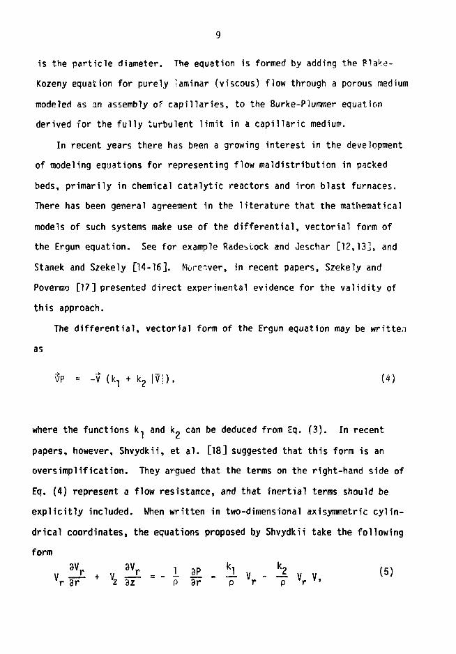
In recent years there has been a growing interest in the development
of modeling equations for representing flow maldistribution in packed
beds, primarily in chemical catalytic reactors and iron blast furnaces.
There has been general agreement in the literature that the mathematical
models of such systems make use of the differential, vectorial form of
the Ergun equation. See for example Radestock and Jeschar [12,13], and
Stanek and Szekely [14-16]. Moreover, in recent papers, Szekely and
Povermo [17] presented direct experimental evidence for the validity of
this approach.
The differential, vectorial form of the Ergun equation may be written
as
fa = -1 (^ + k2 |7|), (4)
where the functions k. and k~ can be deduced from Eq. (3). In recent
papers, however, Shvydkii, et al. [18] suggested that this form is an
oversimplification. They argued that the terms on the right-hand side of
Eq. (4) represent a flow resistance, and that inertia! terms should be
explicitly included. When written in two-dimensional axisymmetric cylin-
drical coordinates, the equations proposed by Shvydkii take the following
form
V 9r z 3z P dr p r p V '

10
and
V 3r vz 3z p 3z p vz p V *
where
V = (Vr2 + V 2
2 ) 0 ' 5 . (7)
They did not present a numerical solution of the full set of equations
containing these inertial terms, but assumed irrotational flow, making it
impossible to corvare directly the results obtained from the two differ-
ent formulations given by Eq. (4) and Eqs. (5-7).
Choudhary, Propster and Szekely [19] have performed numerical experi-
ments to allow direct comparison of the two flow models. They noted that
in contrast to the laminar Navier-Stokes equations, where one would
expect the inertial terms to predominate at high velocities (and at a
distance from solid surfaces), the terms on the left- and right-hand
sides of Eqs. (5) and (6) are both of the order (V ), making it
impossibly to draw conclusions readily regarding the relative importance
of these terms. As expected, the two solutions are essentially identical
for parallel flow through uniformly packed beds. As a critical test,
they performed an isothermal flow analysis of a blast furnace with
alternate "V" shaped layers of different size packing, where the fluid
was introduced through a side stream nozzle (perpendicular to the exit
flow direction). They reported that the two flow models gave quite
similar results, with the differences between calculated point values of
the velocity ranging from 2 to 12%. They concluded that the calculated
difference would be difficult to detect experimentally. The inclusion of

11
these irertisl terms greatly increased the computational labor, and they
questioned whether the refinement in the calculation justified the
additional effort for the majority of engineering calculations. It can
be noted that the flow maldistribution in the blast furnace problem is
more extreme than would be expected in a pebble bed nuclear reactor core,
even with radial power peaks and hot-spot formation.
Early pressure drop studies through sphere beds intended to mock-up
pebble bed reactors indicated, however, that the Ergun equation consider-
ably over-predicts the pressure drop in the Reynolds number range of
interest. Defining a friction factor
APf =
offers a basis for comparison of the Ergun equation with pressure drop
data from Denton [20] and the ORNL Pebble Bed Reactor Experiment (PBRE)
[21]. Figure 3 shows this comparison in a plot of friction factors
versus Reynolds number. The Reynolds number used throughout this paper
is based on the superficial mass flux, G = pV, and the pebble diameter,
d , so thatP
G dDNRe = y * <9>
C. Packed Bed Heat Transfer
The rate of heat transfer in a generating, conducting porous medium
with a flowing fluid phase is controlled by a number of mechanisms,
including bulk movement of the fluid, conduction in both the solid and
fluid phases, convective transfer between phases, dispersion of the fluid
in the interstices of the porous medium, and in the case of a gaseous

12
SPHERE BED FRICTION FACTORS
OogJ5OE-*U
1O 1 -
4*10°
LEGEND° ORNL PBRB DATA (0.394 < e < 0.401)
— DENTON'S DATA (MEAN LINE, c = 0.37)— ERGUN EQUATION (t = 0.39)
1 0 1 0REYNOLDS NUMBER. NRe =
Fig. 3. Comparison of the Ergun equation with datafrom sphere bed flow experiments. The ORNLPBRE data was taken on a series of bedsassembled by different methods in the samevessel.

13
fluid, radiant exchange. Because of the complexities of the solids
packing and the interconnected interstitial spaces, a porous medium
approach to thermal modeling is required. Thus, the dependent variables
are the average temperature of the pebble surface and local value of the
coolant bulk (mixing cup) temperature.
Several investigators have derived differential equations for these
temperatures from thermal energy balances on the solid phase, on the
fluid phase, or on a unit volume of the bed containing both phases.
Choudhury [22] has derived ordinary differential equations in his study
of porous-metal nuclear fuel elements, assuming uniform generation,
constant coefficients and negligible radiant heat transfer. Experimen-
tally determined effective thermal conductivities were used. Singer and
Wilhelm [23] have derived vectorial differential temperature equations
for packed bed chemical reactors, and have presented analytical solutions
for certain restricted cases where constant coefficients can be assumed
and some terms can be neglected.
There are numerous correlations and models in the literature for
packed bed heat transfer coefficients and effective conductivities. One
review by Barker [24] lists 244 references on subjects related to heat
transfer in particulate systems, including fluid-to-particle heat trans-
fer coefficients, mass transfer coefficients, mixing studies and effec-
tive conductivity experiments.
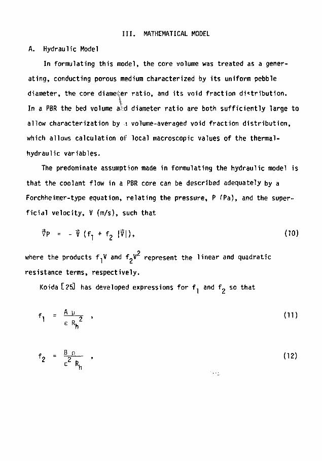
III. MATHEMATICAL MODEL
A. Hydraulic Model
In formulating this model, the core volume was treated as a gener-
ating, conducting porous medium characterized by its uniform pebble
diameter, the core diameter ratio, and its void fraction distribution.\
In a PBR the bed volume af;d diameter ratio are both sufficiently large to
allow characterization by i volume-averaged void fraction distribution,
which allows calculation of local macroscopic values of the thermal-
hydraulic variables.
The predominate assumption made in formulating the hydraulic model is
that the coolant flow in a PBR core can be described adequately by a
Forchheimer-type equation, relating the pressure, P (Pa), and the super-
ficial velocity, V (m/s), such that
fa = - tf (f, + f2 |tf|), (10)
pwhere the products f,V and f_V represent the linear and quadratic
resistance terms, respectively.
Koida [25] has developed expressions for f, and f. so that
, = 4-s- , (IDe R h
Ve

15
where
A and B = empirical coefficients that are constant for a given
particle shape,
R. = effective hydraulic radius for the flow within the packed
bed (m),
e = bed void fraction,
u = fluid dynamic viscosity (Pa«s), and
P = fluid density (kg/m ).
R. for a randomly packed bed of spheres is given by [26]
where d = pebble diameter (m). Equation (10) clearly neglects body
forces (gravity) and does not explicitly include the inertial terms. The
body forces may be safely ignored, as their effect is negligible for the
high gas velocities considered here. It is assumed that the inertial
terms can be safely ignored following the study of Choudhary, et al. [19]
discussed in the previous chapter.
Numerical values for the constants A and B in Eqs. (11) and (1?) of
24.5 and 0.1754, respectively, were calculated using Barthels [27] fric-
tion factor correlation for high Reynolds number gas flows in packed
sphere beds. Equations (10), (11) and (12) and Barthels correlation can
now be expressed as the friction factor defined by Eq. (8). Figure 4
shows the comparison of these friction factors versus Reynolds number
with the information previously displayed in Fig. 2. This model should3 4
not be applied outside the range 10 < Npe < 4 x 10 .
If the fluid pressure drop and temperature rise across the bed result
in an appreciable change ir fluid density, it is more convenient to

16
SPHERE BED FRICTION FACTORS
O
O
S5O
o
1 0 1 -
4*10°
LEGEND«> ORNL PBRE DATA (0.394 < e < 0.401)
DENTON'S DATA (MEAN LINE, c = 0.37)ERGUN EQUATION (c = 0.39)BARTHELS CORRELATION (e = 0.39)THIS MODEL (e = 039)
1 0 4
REYNOLDS NUMBER, NRe
Fig. 4. Comparison of the new flow model withother models and experimental data.The ORNL PBRE data was taken on a seriesof beds assembled by different methodsin the same vessel.

17
calculate the mass flux, G = PV, rather than the fluid velocity. Using
G, Eq. (10) becomes
VP = - G" ( g , + g 2 | £ | ) , (14)
where
Since curl grad = 0, the pressure variable can be eliminated from Eq.
(14); thus
^X [- G* ( 9 l + g 2 | S | ) ] = 0 . (17)
The model's equations have been formulated in axisymmetric cylin-
drical coordinates because they allow a realistic representation of
actual physical conditions, and facilitate coupling of this model to the
current neutronics model. Manipulation of Eq. (17) yields the following
scalar equation
-57T - (g-i + g? |G|) G
were z1 and r' are the axial and radial coordinates.
] - r [- (9, + 92 |fc|) Gz] = 0. (18)
The equation is made nondimensional by the appplication of the
following definitions:
. inGg2
GIN
GIN
2 92IN
r = -p- , z = j-- , and a = j- ,
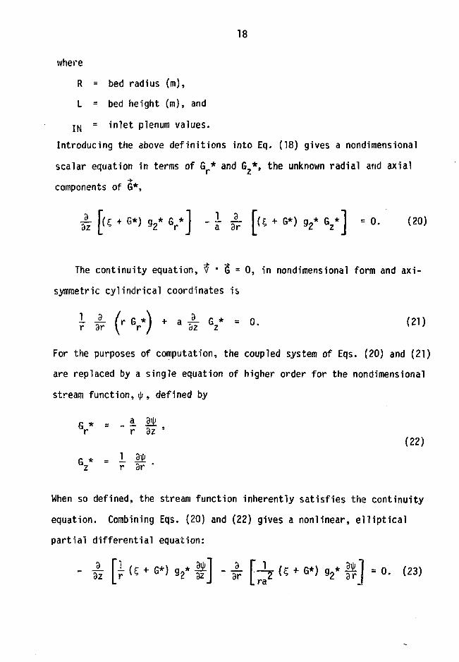
18
where
R = bed radius (m),
L = bed height (m), and
IN = inlet plenum values.
Introducing the above definitions into Eq. (18) gives a nondimensional
scalar equation in terms of Gr* and G2*, the unknown radial and axial
components of G*,
£ [(£ + 6*) g2* Gr*l - I A F(4 + G*) g2* Gz*l = 0. (20)
The continuity equation, v* * 5 = 0, in nondimensional form and axi-
symmetric cylindrical coordinates is
F W (rGr*) V 'For the purposes of computation, the coupled system of Eqs. (20) and (21)
are replaced by a single equation of higher order for the nondimensional
stream function,^, defined by
G * = - ir r
* = 1 Jiz r 3r
(22)
When so defined, the stream function inherently satisfies the continuity
equation. Combining Eqs. (20) and (22) gives a nonlinear, elliptical
partial differential equation:

19
Because the coefficients are a function of temperature, and the temper-
atures in turn depend on the mass flux, a complete thermal-hydraulic
description results in a set of coupled elliptic partial differential
equations like Eq. (23). The numerical solution method selected [28]
requires that the equations be expressed in terms of the nondimensional
variables in the following form (See Appendix A):
h (•£)-£(•£)]- &[-•'&(<••)]i , i (c cjYI + rdA = 0 , (24)
b 2 9 r V <t> / <ba \ ' J
where <J> is the dependent variable,
ip is the stream function, and
a., b,, c,, and d, are functions used as required to make Eq. (24)
and the equation transformed identical.
For Eq. (23), the following functions are used:
0 = \|>, a, = 0, b, = (E, + G*)gp*» and c, = 1. (25)
Equations (23) and (24) are expanded and set equal to each other to
obtain the expression for d,. The resulting general nondimensional form
of Eq. (23) becomes
l - A l"_r_j 3r ^21 [ r (r + G*) a * 4 l - A l_r_ (E + G*) a *9Z j r u + fa ; g2 9 z j 3 r ^ 2 u + t. ; g2
+ \ U + G*) g2* |£ = 0. (26)a

20
Once the stream function field is obtained, the pressure distribution
follows. Computing the divergence of Eq. (14), with application of the
continuity equation, and applying the nondimensional definitions yields
the following scalar equation:
JL / X <¥1\ _L L 9P*9r ^ 2 3r I 3z ^r 9z
(27)
- If £
were P* = P/Pre*» the nondimensional pressure. Equation (27) is in the
form of Eq. (24) where
((> = P*, a. = 0, b, = c, = 1, and
(28)
Using the coupled set of Eqs. (26) and (27), one can solve for the pres-
sure and velocity distributions within the confines of the bed.
B. Thermal Model
The rate of heat transfer in a generating, conducting porous medium
with a flowing fluid phase is controlled by a number of mechanisms,
including bulk movement of the fluid, conduction in both the solid and
fluid phases, convective transfer between phases, dispersion of the fluid
in the interstices of the porous medium, and radiant exchange. When
different mechanisms have a common driving potential, they may be com-
bined by applying an effective heat transfer coefficient.

21
The macroscopic temperature gradient in the solid phase drives a
complex group of heat transfer mechanisms, which operate both in parallel
and in series. These include thermal conduction through the solid peb-
bles, conduction through the stagnant fluid film near the contact point
of two adjacent pebbles, thermal conduction by contact between pebbles
and for a gaseous fluid, radiant heat exchange. The net effect of these
mechanisms can be expressed by an effective thermal conductivity coef-
ficient for the solid phase, k . The static term, k° derived by
Kunni and Smith [29] is used in the model, given by:
k°/kf = e (1 + 3Nurv) + 3 (1 - e)/M/(j+Nurs)+Y^J. (29)
where
kf = fluid molecular thermal conductivity (W/m*K),
k = solid thermal conductivity (W/m«K)
0 = geometry factor, here equal to 0.95, and
Y = geometry factor, equal to 2/3 for spheres.
Nu and Nu are Nusselt numbers for radiant heat exchange between
void spaces and between solid surfaces:
= hrv V ¥ hrv
(31)*rs "rs ~ D ' " f ' "rs ""-«? • v_r- • \%"i
where e r is the solid surface emissivity and o is the Stephan-
Boltzmann constant, and t is the pebble average surface temperature (K).

22
The empirical factor, <J>, is calculated from:
* = 4>2 + (^ - 4>2) (e - 0.260)/0.216. (32)
When e < 0 .260 ,4> = <f>2- When e > 0 . 4 7 6 , <J> = <ty *1 and <t>2 a r e
given graphically in [29]. Curve fits of these parameters [30] are used
here. For the range
10 < i-5- < 300,kf
/k, \ 0.2426= 0.2770 f f- J , (33)f
vz - 0.1293 , k f \ 0-3292(
In the fluid phase, heat is transferred between fluid regions at
different temperatures by two mechanisms: molecular conduction and
turbulent dispersion in the interconnected interstitial voids of the
solid phase. These combined effects are approximated by a single effec-
tive thermal conductivity coefficient for the fluid phase [23] given by
k f e = e kf + p cE , (34)
where
c = fluid specific heat capacity at constant pressure (J/kg-K), and
E = turbulent thermal diffusivity of the flowing fluid phase
(m2/s).
Because the turbulent thermal diffusivity is anisotropic, the fluid
effective thermal conductivity is also anisotropic. The axes of interest
(r,z) coincide with the axes of the principal effective thermal conduc-
tivities.

23
The numerical values of E are calculated using the method suggested
by Finlayson [31]. The turbulent Peclet number is defined as
N p e - -^ (35)
Finlayson suggests that the radial and axial variations in the local
value of E can be correlated with variations in the axial fluid velo-
city, Vz, such that
frVz
r=r"Pe,r
and
E
V2
2 " " (36)NPe,z
z=zThe radial and axial turbulent Peclet numbers can be easily changed
in the code. At present the radial and axial values are 10 and 2, re-
spectively. These values assume the turbulent thermal diffusivity is
numerically equal to the turbulent mass diffusivity. The turbulent
Peclet numbers above correspond to "consensus" values reported by Deans
and Lapidus [7].
The distributions of local fluid bulk temperature and pebble average
surface temperature can be obtained by the solution of equations derived
from thermal energy balances on the two phases. These balances are based
on the fluid superficial velocity and the total cross-sectional area.
Convective coefficients, generation rates, and thermal conductivities are
corrected for the proper fraction of the bed. A thermal energy balance
on the solid phase results in the following equation:
^ ' (" kse V + h av (ts " V* ' q =
24
where
h = corrective heat transfer coefficient (W/m «K),
a = pebble surface area per unit volume of the bed <m~ ),
t, = local value of the bulk temperature of the interstitial
fluid (K),
t = local value of the pebble average surface temperature (K), and
q = energy release rate per unit volume of the bed (W/m ).
The terms in Eq. (37) represent, from left to right, effective conduction
in the solid phase, convective transfer between the phases, and internal
generation from fission and decay. Introducing the following nondimen-
sional variables
T - A . T -JL C^± kfeC K
lfIN KfIN KfIN
kKs = \r~ ' V = av u h*= ir1 - -andS KfIN V V K
vfIN ¥ v *fIN *fIN
allows Eq. (37) to be transformed by the same methods and definitions
used to obtain Eq. (26). The result, in axisymmetric cylindrical coor-
dinates is
S I s i s i r s i I I
which is in the appropriate general nondimensional elliptic form required
by the numerical solution technique.
Peterson [32] has shown that for helium, the specific heat at con-
stant pressure, c, can be assumed constant for engineering purposes.

25
Assuming c constant, a similar treatment of the thermal energy balance
for the fluid phase yields
[te \f 3r/ 9r \'f dz
] -] [ ] V9z ' lvfz 9z 9r 2 lxfr 9r "" "v
where it should be noted that the effective thermal conductivity coef-
ficients are anisotropic.
Values for the convective heat transfer coefficient, h, are obtained
from the Jeschar correlation [33] for the Nusselt number, which is
applied locally:
h d r n , -i 0.5 N D oN = -r-^ = 2.0+ ~? N D + 0.005-^-, (41)
f |_ e I
where the Reynolds number, based on the superficial velocity and the
particle diameter, d , is given by
NRe - ^ V (42)
The Nusselt number correlation is reported to be valid for ReynoldsA
numbers between 250 and 5.5 x 10 .
The effective thermal conductivities of the solid and fluid phases
are functionally related to the local film temperature, usually the
arithmetic average of tg and tf. This dependence of the coefficients
on the dependent variables makes Eqs. (39) and (40) nonlinear.

26
The computer code based on this model solves Eqs. (26), (27), (39),
and (40) as a coupled system of nonlinear elliptic partial differential
equations. Boundary conditions for the solution of a selected physical
system are specified at r = 0, r = 1, and both z limits (inlet and
outlet) which need not be parallel.
Once the numerical solution has converged and the pebble average
surface temperatures have been obtained, the internal temperatures and
temperature gradients can be calculated. Referring to Fig. 2, let
r. = radius of inner fueled/unfueled interface (equal to zero for
the conventional ball),
r_ = radius of outer fueled/unfueled interface (m),
r» = pebble radius (m), and
Q = power per ball (W/ball).
For the conventional element, the temperatures at r, and r? are given by
+ *2 • (43)
and
t2 = J&- (i- - Th) +tc. (44)
The temperature gradient at the fueled/unfueled interface is given by
dt _ -Q
For the shell ball
r , „ 2 . 2
(r23-r

27
with t? given by Eq. (44). The temperature gradient at the outer
fueled/unfueled interface is given by Eq. (45).
The thermal conductivity of the pebble is a function of temperature
and integrated fast neutron flux. Lacking a thermal conductivity model,
a curve fit to an axial distribution corresponding to an idealized OTTO
fuel cycle [34] is used in the code. It is assumed that the thermal
conductivity of the fueled matrix and unfueled graphite are equal. The
function used to fit the data is
ks(z) = 17. + 20.5 e"15>37z (47)
The resulting distribution is shown in Fig. 5.

28
PEBBLE THERMAL CONDUCTIVITY40 O
>
oDQ
O
u
3C
35 0
30 • 0 -
25 • 0 -
2 0 0 -
15 00 0 0 2 0-4 0-6 0 8 1 0DIMENSIONLESS AXIAL POSITION , z / L
Fig. 5. Distribution of pebble thermal conductivitycorresponding to an idealized OTTO fuelcycle.

IV. COMPUTER CODE PEBBLE
A. Solution Technique
The finite difference equations used in program PEBBLE were derived
from the differential equations of the mathematical model by integrating
over finite areas, based on as:umed distributions of the variables be-
tween the nodes of the grid [28,35]. This approach ensures that conser-
vation laws are obeyed over arbitrarily large or small portions of the
field. In addition, this approach is most appropriate for the macro-
scopic porous medium model of a packed sphere bed, which already includes
the assumption that the variables in a given bed volume are well charac-
terized by macroscopic average values.
The coupled system of nonlinear algebraic equations is solved by a
point iterative method, with the option of under or over-relaxing the
dependent variables as necessary. A Gauss-Seidel method is used, in
which the new values are used in each iteration cycle as soon as they
become available. This method is known to yield rapid convergence and
places low demands on computer storage. Details of the derivation of the
finite difference equations from their differential counterparts, along
with details of the successive substitution formulae can be found in
Appendix A. This method is a modification of the techniques developed by
Gosman, et al. [28]. The code is written in modular form, with the
finite differencing being done by the code. This allows great flexi-
bility, in that equations can be easily changed or added.
The user has the option of using either upwind or central differences
for the advective terms (those terms multiplied by a^ in Eq. 24).
Central differences are more accurate, but upwind differences may be
required to ensure the convergence of some equations. This will be

30
discussed further in Chapter VI. Properties are updated at the end of
major iteration cycles, and the mesh can be swept for an equation as many
times as desired within each major iteration cycle. References are given
in the code for property models. A subroutine solves the Beattie-
Bridgeman equation of state to recover the coolant density at each prop-
erty update.
The convergence criterion used dictates that the maximum fractional
change in a dependent variable, <l>, in the field must not exceed a pre-
scribed value, that is
[(•<«> - •<"-»)/•<«]..„ -<«• <«>where the bracketed superscripts denote the values for the Nth and Nth-1
iterations, respectively. Tests with PEBBLE have shown that changes in
calculated values are insignificant for cc < 0.005.
To recover the mass flux at the axis of symmetry, we note that for a
finite mass flux, the radial derivative of the stream function, ty, must
approach zero at the same rate as r near the axis. It follows that
the $ 'v> r distribution is parabolic near the axis. The program assumes
this relationship holds at grid points once and twice removed from the
axis, allowing the mass flux, G*, to be calculated at r = 0. The mass
flux, G*, is set equal to zero at the impervious wa?l to approximate the
no-slip condition. The presence of G* in the resistance coefficient,
however, then incorrectly leads to a reduced resistance to flow adjacent
to the wall. In the code, therefore, it is assumed that the flow resis-
tance at the radial boundary node is the same as the resistance at the
adjacent interior node.

31
The code does not require rectangular boundaries at the z limits of
the bed (inlet and exit). The boundaries are set with the arrays I INLET,
IMIN, IMAX and IEXIT. The successive substitution formula is only
applied from IMIN to IMAX. The code does assume that the grid is defined
so that grid points lie on the boundaries. If the user wants to incorp-
orate non-rectangular boundaries, changes will need to be made in sub-
routines GRID and BOUND, and MFLUX should be checked.
The code is heavily commented and referenced, and was written to be
used by others. A listing of the code, as set up for a coupled thermal-
hydrualic test problem, r> provided as Appendix B. The thermal-hydraulic
test problem is discussed in Chapter VI.

V. ORNL PBRE ANALYSIS
A. Pebble Bed Reactor Experiment
Though the ORNL PBRE was never built, a full-scale mockup was con-
structed and extensive velocity and mass-diffusion measurements were
made [21], The PBRE was designed to be a 5 MW(t) all ceramic, helium-
cooled pebble bed reactor system, with the core volume containing approx-
imately 11700 spherical fuel-moderator elements [36].
The mockup used unfueled graphite spheres, 0.0381 m in diameter,
loaded in a Plexiglas core model. The cylindrical core had an inverted
conical core support plate with an included solid angle of 120 , which
had a central 120° conical ball discharge dome. A free-surface fill
cone at the angle of repose topped the bed. The basic geometry is shown
in Fig. 6. The core had a diameter of 0.762 m, giving a bed to ball
diameter ratio of 20. For experimental Bed 13 (modeled in this paper),
the height from the lowest point of the core support plate to the peak of
the fill cone was 1.35 m. Air was supplied to a plenum structure below
the slotted core support plate, flowed upward through the interstitial
voids in the bed, and exhausted to atmospheric pressure above the fill
cone.
Point velocities vsre measured above the bed with a hot-wire anemom-
eter, and averaged over all angular measurements at each radial position
to give the mean radial velocity profile. The velocities measured cor-
respond to superficial velocities, and the angular averaging makes com-
parison of measurements with an axisymmetric cylindrical coordinate
prediction reasonable.

PHYSICAL BED vs . NUMERICAL MODEL
ATMOSPiCRlC PRFSSURl .•
SLOTTED COHESUPPORT PLATE
INLET PL E M M
F 1 N 1 - OlFfEBENCE OO1D
DIHEUSIONLtSS RADIUS
COCo
Fig. 6. The basic geometry of the ORNL PBRE is shown at the left. The lettersE, I, FT and FC denote the location of the exit faces above whichmeasurements were made. The corresponding finite difference grid isshown at the right.

34
Once a bed was constructed and measurements had been made above the
fill cone, graphite spheres were removed to form flat-topped beds at
three axial positions. Referring to Fig. 6, FC denotes the location of
measurements taken above the fill cone, FT denotes the flat top configu-
ration with the fill cone removed, I denotes the intermediate configu-
ration with the upper half of the bed removed, and E denotes the bed
configuration where only the entrance region was filled with spheres.
For each bed, the flow rate was varied to give Reynolds numbers, based on
the pebble diameter and superficial velocity, between 1150 and 9400. The
small bed to ball diameter ratio, and complicated inlet geometry caused
some modeling difficulties, but the PBRE mockup measurements offer the
only experimental data available for relatively large packed beds of
large, uniform-diameter spheres with an interstitial fluid flowing at
high Reynolds numbers.
B. Code Validation Concerns
Normally, code validation relies on analytical solutions, or data
from geometrically simple experiments; in this case, no two-dimensional
analytical solution could be obtained, and no simple experiment was
available. The only comparison that has been made vith a known solution
involved modeling an isothermal, uniform-property bed. With constant
pressure conditions at the inlet and outlet, this configuration should
yield a uniform velocity profile (plugflow). The plugflow calculation
uses a rectangular grid, modeling an axisymmetric cylinder with flat,
constant-z inlet and outlet faces, having a uniform void fraction of
0.39. The pressure boundary conditions are based on symmetry at r = 0
and r = 1, and constant pressure at the inlet and outlet, with the inlet

35
face value specified at 1.0. Boundary conditions on ^ at both the inlet
and outlet correspond to parallel, axial flow (i.e. 9^/3z = 0). The axis
of symmetry and impervious radial wall must both be lines of constant <K
Because the introduction of \\> increased the order of the original dif-
ferential equation, one of the \l> boundary conditions is arbitrary. For
numerical simplicity, we chose the value of \\> = 0 at r = 0 for all z.
Once the value of \p has been set at r = 0, the ty distribution for
plugflow can be determined from Eq. (22), by setting G * = 1 and inte-2
grating from r = 0 to r = r. Thus for plugflow, <JJ = 0.5 r . This
function is shown in Fig. 7. The wall values of t/i can then be set at
0.5, which ensures that the area-averaged dimensionless mass flux across
each bed cross-section equals unity [16]. For this configuration, pro-
gram PEBBLE calculated uniform velocity flow. The calculated pressure
distribution was consistent with a one-dimensional form of the governing
equation. The solution is well behaved, converging in a stable manner
regardless of the initial guess.
With confidence in the numerical technique gained from the' plugflow
calculation, the ORNL PBRE mockup was modeled with PEBBLE. The radial
boundary conditions on i> and pressure are the same as for the plugflow
case. The boundary conditions on i|> at the inlet and outlet correspond to
flow perpendicular to the face; the condition being that the normal
derivative of ty is zero. The boundary condition on pressure at the
outlet specifies the value of 1.0, the reference value. In the solution
reported previously [37], the boundary values of pressure at the inlet
were computed using the calculated normal pressure gradient at the inlet,
the appropriate area-averaged value of the pressure for the adjacent
internal nodes, and the appropriate distance normal to the inlet

36
STREAM FUNCTION FOR PLUGFLOW0 6
-0 100 02 0 4 06 08 10
DIMENSIONLESS RADIAL POSITION , r / R
Fig. 7. The radial distribution of \\> for plugflow.

37
face. As reported earlier, for Bed 13FCa this resulted in an apparent
error in the calculated core pressure drop of 5.5%, and the calculated
pressure distribution near the inlet did not vary smoothly. Application
of this boundary condition later yielded an obviously incorrect solution
for the coupled thermal-hydraulic problem. It was found in the liter-
ature [35] that this plausible (and physically correct) technique is
known to cause numerical problems. Since the inlet boundary condition
on \p assumed flow normal to the face, the pressure had to be constant
along the face for a physically correct solution. The new boundary
technique involves applying the above condition at one point, and then
setting the pressure at all inlet boundary points to that value.
The finite difference grid was set up with a constant Ar and a var-
iable Az, so that grid points fell on the inlet and outlet boundaries.
Bed 13FC was calculated "n a 21 x 51 grid. The grid definition and
outlet boundary conditions were then adjusted to model Beds 13FT, I, and
E. Bed 13E was calculated on a 21 x 16 grid. The grid for Bed 13FC is
shown in Fig. 6.
A relaxation parameter of 1.285 was used for the calculation of ty; a
value of 1.0 was used for the pressure recovery calculation. Calculation
of Bed 13FCa for cc = 0.005 required 31 s of CP time using a CDC 6600
computer, the interactive NOS operating system, and the LASL FUN compiler.
C. Void Fraction Distribution in the PBRE
The void fraction, e, in a cylindrical packed bed only achieves the
random packed bed value of 0.39 for very large beds. Since a sphere
makes only point contact with the wall, the void fraction varies from 1.0
at the wall to a minimum at one-half ball diameter from the wall. Its

38
value then oscillates before approaching a constant value 5 to 10 ball
diameters from the wall [38-40]. Bundy [2l] measured the total void
fraction of Beds 13FT and 13E, reporting values of 0.401 for Bed 13FT,
and 0.366 for Bed 13E. The void fraction distribution used by PEBBLE for
the cylindrical portion of the bed is shown in Fig. 8. This distribution
is based on the DD ./d = 14.1 data of Benenati and Brosilow [38],Bed p
modified by data from measurements on one-fourth scale PBRE models by
Thadani and Peebles [39], The fill cone void fraction was set to the
nominal value of 0.401, as no data are available for free-surface fill
cones.
The porous medium model is difficult to apply in the entrance region,
which has numerous structural surfaces and contains a relatively small
number of spheres. Bundy [21] measured a large void fraction in the
lowest part of the entrance region, a low value higher in the region, and
a mean value of only 0.366 for Bed 13E. It was believed that the large
value was a result of the wall effect, with spheres in only point contact
with the structure, while the low value was a result of rhombohedral
close-packing (e = 0.26) at the bottom of the cylindrical bed.
Wadsworth [41] had previously observed rhombohedral packing near the
bottom of flat-bottomed beds.
In the absence of detailed information on the distribution of e in
the entrance region, the void fraction distribution assigned to this
region in PEBBLE was manipulated to give the approximate shape of the
reported velocity profiles causing the flow to enter the calculational
bed in approximately the same manner as it had entered the experimental
bed. The resulting distribution used the area void fraction of the core

39
(0
O
VOID FRACTION DISTRIBUTION0 70
0 65
0 60
0 55
0 50-
0-45-
O> 0 40 -
0 35-
0 X
• LOCAL VOID FRACTION . cVOLUME INTEGRATED (from wall)
2 4 6 8BALL DIAMETERS FROM WALL
10
Fig. 8. Void fraction distribution used inPEBBLE to model the cylindricalportion of PBRE Bed 13.

40
support plate (including no-flow regions) for the value of e at the
boundary and the first two internal grid points (about one-half ball
diameter). Next, a layer of rhombohedral close-packing, one ball
diameter thick, was assumed for the regions above the discharge dome and
the slanted core bottom. The void fraction of the remainder of the
entrance region was set to the measured mean value of 0.366.
D. Comparison of Predictions with Measured Values
Figures 9 and 10 display predictions by PEBBLE for the distribution
of stream function, pressure and velocity in Bed 13FCa of the PBRE mockup
series. Some general observations can be made concerning these figures.
The streamlines are perpendicular to the isobars. When bed properties
change, such as in the entrance region or the fill cone, the flow redis-
tributes in very short distances. In the cylindrical portion of the bed,
where the void fraction in the model varies only radially, the
streamlines are parallel and the flow is purely axial. The pressure
gradient is steeper in the entrance region, where there is denser pack-
ing, than in the remainder of the bed.
Pressure data for the PBRE mockups were reported in the form of
friction factors. For Bed 13FCa, with an inlet Reynolds number of 6275,
the reported value was 5.59. With the inlet boundary technique disclosed
in Section B of this chapter, PEBBLE calculated a value of 5.607. The
print output for the analysis of Bed 13FCa is provided as Appendix D.
Figures 11 through 14 compare predictions by PEBBLE for the exit
velocity profiles of Beds 13E-FC with those measured on the full-scale
mockups. The calculated velocity profile at the exit face of the en-
trance region of Bed 13E, resulting from the void fraction distribution

STREAMLINES AND ISOBARSM A S S F L U X S T R E A M L I N E S . PBRE BED I3FCA
1
f
f
Hi
[;
y
V.
\
>
i
1
D1MENS1ONLESS R«O1US
ISOBARS <NOBM«LUE0>. P8BE 8E0 I3FC«
B - — B 8 » -
OlMtNSIONLESS RAOIUS
Fig. 9. Calculated mass f lux streamlines and isobars for PBRE Bed 13FCa.Contour values correspond to \\i - 0.5 r2 in steps of 0 . 1 , wherecontour A is zero. Pressure contour values range from A = 1.0to K = 1.031 and are equally spaced.

VELOCITY PREDICTION FOR OAK RIDGE PBREFILL CONE TOPPED BED 13FCaTHICK LINES MAP BED LIMITS
INLET REYNOLDS NUMBER = 6275
Fig. 10. Calculated distribution of normalized velocity for PBRE Bed 13FCa.

43
and inlet boundary conditions discussed in the previous sections, is
shown in Fig. 11 with the corresponding experimental data. Figures 12
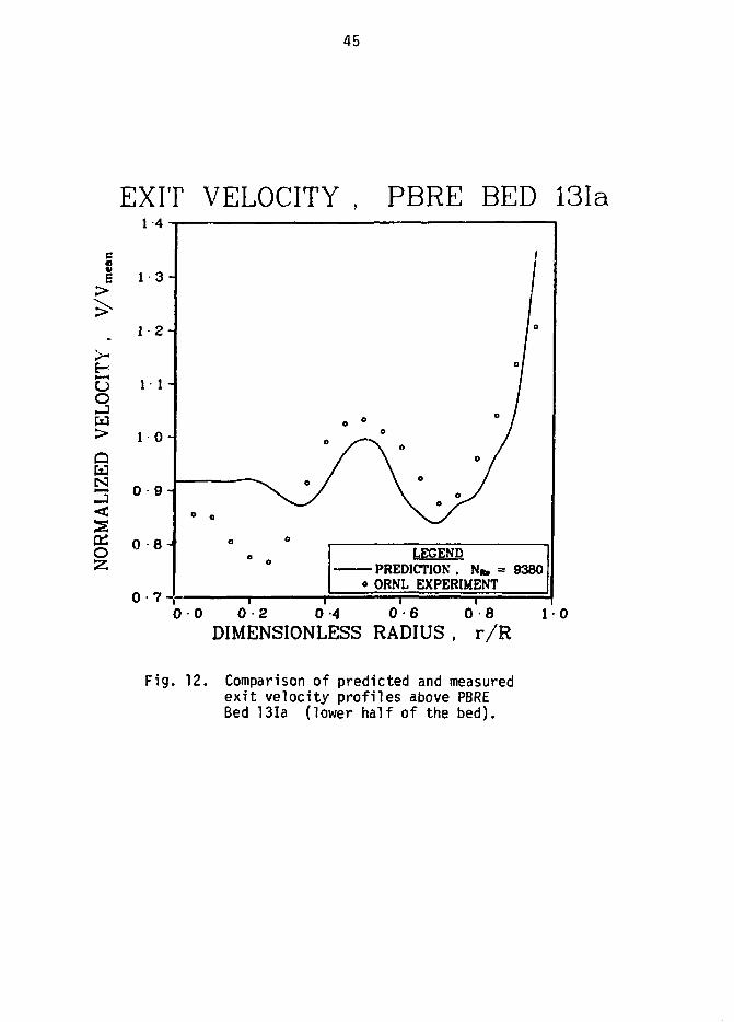
and 13 demonstrate that the calculated velocity profiles for Beds I and
FT are essentially the same, which is consistent with Fig. 9. The dif-
ferent shape of the experimental velocity profiles at the two locations
may be caused by axial variations in the bed packing. Wadsworth [41] has
noted that axial variations in the void fraction distribution can exist,
but none were modeled here because no data are available. The agreement
between predicted and measured velocities for Bed 13FT, shown in Fig. 13,
appears excellent, at least for an inlet NR of 8555 (see also Fig.
17). Note, however, that other choices could have been made in assigning
the distribution of e in the cylindrical portion of the bed; a different
distribution would change the shape of the calculated velocity profile.
The void fraction distribution shown previously in Fig. 8, while having
the correct characteristics in an overall sense, may be locally
inaccurate. Differences probably exist between PBRE Bed 13, formed from
the previous bed by through-cycling 12710 spheres [21], and the very
small scale beds used for the measurement of void fraction distribution.
These small scale beds were formed by simply dumping spheres into a
cylindrical volume [38-40].
Calculated and measured velocities above the fill cone are compared
in Fig. 14. The calculated velocity profile is in good agreement with
the experimental measurements. Since the entire fill cone region was
assigned a uniform void fraction of 0.401 in the numerical model, the
good agreement between the measured and calculated FC velocity profiles
is probably not the result of a fortunate choice of void fraction distri-
bution. The results shown in Fig. 14, therefore, indicate that the

44
EXIT VELOCITY , PBRE BED 13Ea
oW
aw
gz
i • o -
1 2 -
1 1 -
1 0 -
0 9-
0 8-
0 7-
0 6-
0 5-
O
/
o y
J LEGENDPREDICTION . NB, = 6485
• ORNL EXPERIMENT" i i i
0 - 0 0 2 0 4 0 6 0 8 1 0DIMENSIONLESS RADIUS , r/R
Fig. 11. Comparison of predicted and measuredexit velocity profiles above PBRE Bed13Ea (entrance region).
45
EXIT VELOCITY , PBRE BED 131a1 4
V * m
ean
-
>-HUOw
QM
1
1
1
1
3 -
• 2 -
1 -
0 -
~ 0 9-
0 8
0 - 7 J
LEGENDPREDICTION . NM = 9380
• ORNL EXPERIMENT
00 02 0 4 06 08 1DIMENSIONLESS RADIUS , r /R
Fig. 12. Comparison of predicted and measuredexi t velocity profi les above PBREBed 131a (lower half of the bed).

46
EXIT VELOCITY , PBRE BED 13FTa
>
Oow
1 3 -
1 2 -
i 1 -
1 0 -
0 9 -O2
0 8
LEGEND- PREDICTION . NR. = 8555ORNL EXPERIMENT
0 0 0 2 0-4 0 6 0 8DIMENSJONLESS RADIUS , r/R
1 0
Fig. 13. Comparison of predicted and measuredexit velocity profiles above PBRE Bed13 FTa (flat-top bed, fill coneremoved).

47
EXIT VELOCITY , PBRE BED 13FCa
s>
VEL
OCI
QuxQ
RMA
LI5
o
1
1
1
1
1
0
0-
0
0
• 0 -
6-
•4 -
2 -
0 -
8 -
6 -
•4 -
2 -
0
/
0 /
/
O /
0 0 /O . /
1 1
LEGENDPREDICTION , NR. = 6275
0 ORNL EXPERIMENTI 1
00 02 0 - 4 0 6 0-8DIMENSIONLESS RADIUS , r / R
1 0
Fig. 14. Comparison of predicted and measuredexit velocity profiles above PBREBed 13FCa (entire bed topped by fillcone).
48
mathematical model and numerical technique used by PEBBLE are appropriate
for the analysis of high Reynolds number flows in packed sphere beds.
Figures 15 through 18 show the effect of inlet Reynolds number on
both prediction and experiment for Beds 13E-FC. Again, the results for
the Bed 13FC are encouraging, but the results for Beds 13E-FT require
further comment. The response of the prediction with respect to Reynolds
number is consistent with the mathematical model. It has been previously
noted by Szekely and Povermo [17] that the profiles should be similar as
long as the quadratic term dominates the resistance to flow. In
reporting the PBRE mockup measurements, Bundy [21] questioned the
apparent Reynolds number effect shown in the data, stating
"...an effect of the flow rate on the shape ofthe velocity profile cannot be clearly deducedfrom the present data, and such an effect of theflow rate, if it exists, must certainly be small.The differences observed in the normalized velo-city profiles measured at the same point above abed at different mean velocities might have re-sulted from changes in the velocity profile be-tween the exit face of the bed and the measure-ment height, which was 9 in. above the bed."
E. Discussion of PBRE Results
A mathematical model and numerical solution technique have been
developed that allow calculation of macroscopic values of the hydraulic
variables in an isothermal axisymmetric pebble bed under steady-state
conditions. The computer code PEBBLE has been shown to predict
distributions of coolant velocity and pressure, limited only by knowledge
of the geometry of the bed.
The lack of detailed knowledge of the local void fraction does not
limit the ability of PEBBLE to perform an accurate thermal-hydraulic

49
EFFECT OF REYNOLDS NUMBER1-3
0 3
LEGENDNR. = 6485
BED 13Ea, NR, = 6485PREDICTION . NR. = 3310
* BED 13Eb . Ng. = 3310
00 02 0 4 0 - 6 08 10
DIMENSIONLESS RADIUS , r / R
Fig. 15. Comparison of predicted and measuredexit velocity profiles above PBRE Bed13E for two different inlet Reynoldsnumbers.

50
EFFECT OF REYNOLDS NUMBER
O 0 7-
0 600 02 0 -4 06 08
DIMENSIONLESS RADIUS , r/R1 0
Fig. 16. Comparison of predicted and measuredexit velocity profiles above PBREBed 131 for two different inlet Reynoldsnumbers.

51
EFFECT OF REYNOLDS NUMBER
E>
OO
Ed>
QW
a:o
i
i
i
I
0
0
0
j 4 -
n• 3 -
2 -
1-
0 -
9 -
8 -
• 7 -
LEGENDPREDICTION . N t e
o BED 13FTa. NR, =PREDICTION, NR«
• BED 13FTb , NR. =
0 „ _ / ^
*
, » •
= B5558555
= 2760= 2760
1
If14
4- 1
of
* 1
///
• /
/^V /\ /
* V * J^
1 |
0 0 0 - 2 0-4 06 08DIMENSIONLESS RADIUS , r / R
1 0
Fig. 17. Comparison of predicted and measuredexit velocity profiles above PBREBed 13FT for two different ir.letReynolds numbers.

52
EFFECT OF REYNOLDS NUMBER2 0
s
ooEd
IZED
NO
RM
AL
1 8 -
1 6 -
1 4 -
1 2 -
1 0 -
0 - 8 -
0 6 -
0 4 -
0 2
LEGENDPREDICTION . N*. = 6275BED 13FCa, N * = 6275PREDICTION . N to = 1175BED 13FCb . N t e = 1175
0 0 0 2 0 4 0 6 0 8DIMENSIONLESS RADIUS , r/R
1 0
Fig. 18. Comparison of predicted and measuredex i t velocity profi les above PBREBed 13FC for two dif ferent in le tReynolds numbers.

53
analysis of large pebble bed power reactors, such as those being designed
by the Institut fur Reaktorentwicklung, Kernforschungsanlage, Julich
(KFA). These large power reactors have bed-to-ball diameter ratios of
about 200, and even have an array of structural depressions in the radial
reflector to minimize, or eliminate, the wall effect. These beds can be
modeled accurately (on a macroscopic scale) by assuming the entire bed to
be characterized by a nominal void fraction of 0.39. In addition, the
combination of the continuous OTTO fuel cycle and coolant downflow en-
sures that very little heat is generated in the portion of the core
adjacent to the ball discharge structure, resulting in nearly isothermal
conditions in this region [42]. Thus, the thermal-hydraulic calculation
is not of critical importance in those regions where its accuracy may be
in question.
Further validation of the flow model will require data from a
geometrically simple flow experiment. The experimental bed should have a
large bed to ball diameter ratio and parallel, constant-z inlet and
outlet faces. Its void fraction distribution should be measured in both
the radial and axial directions. Annular flow dividers should be used
beyond the exit face to minimize the tendency of the flow to return to an
empty tube velocity profile, ensuring that the anemometer measures the
proper velocity. The possibility of using a circular hot-wire in these
annular regions should be investigated.

VI. COUPLED THERMAL-HYDRAULIC TEST PROBLEM
A. KFA Power Reactor Design
The design chosen for the test case is the KFA PR3OOO Design Case
1013. This design was chosen because the axisymmetric power distribution
is available in the literature [34]. Case 1013 is a 3000 MW(t) PBR
operating on a low-enriched uranium (LEU) OTTO fuel cycle The bed
contains approximately 1.8 x 10 shell type fuel-moderator elements,
and has a core-average power density of 9 MW(t)/m . Helium is supplied
to the upper void space at a pressure of 4 MPa, with a mixed-mean temper-
ature of 523 K at the rate of 785 kg/s. All input values for geometry
and design parameters can be found on the third page of the code listing
supplied as Appendix B. The axisymmetric thermal power distribution is
entered in the Block Data Subprogram POWER. Input values, including the
power distribution, can also be found in the print output from program
PEBBLE for this test case, which is supplied as Appendix C.
B. Numerical Model
The physical reactor is assumed to be axisymmetric, and the effects
of the many small fill cones on the upper free surface, and the ball
discharge structures, are ignored. The bed is characterized by an aver-
age height in the design information. A comparison of the physical
reactor and the numerical model is shown in Fig. 19. These approxi-
mations are the same as those used for the neutronics calculation which
supplies the axisymmetric thermal power distribution.
The KFA neutronics code VSOP provides power per ball (kW/ball) at the
volumetric centers of N equal annular volumes. Design Case 1013 was

PHYSICAL REACTOR v s , NUMERICAL
HE AC TO*
AXIS OFSTMMEItV
I N l l l PLENUM
BCD
I oimnI
MODI I
Fig. 19. A comparison of the physical reactor and the axisymmetric model usedin the analysis.

56
calculated on 18 equal radial volumes. The resulting radial grid spacing
can be seen in Fig. 20. Power per ball values are available for radial
locations 4-21 (22 total radial points). PEBBLE was originally set up
using the finite difference grid shown in Fig. 20, where the extra grid
lines near the axis of symmetry were added to aid in the calculation of
G* at r = 0 (See Chapter IV). This grid resulted in a false flow
maldistribution being calculated in the region of radial lines 4 through
7 (verified by another plugflow test). The grid spacing need not be
uniform, but neither can it be too coarse. It is noted that the calcu-
lation of Gz* requires the radial derivative of a function something
like that shown in Fig. 7. PEBBLE now includes the subroutine INTERP
which interpolates the VSOP input to equally spaced radial grid points
for the thermal-hydraulic calculations. It would be possible to use
INTERP to interpolate the thermal-hydraulic variables back to the VSOP
spacing if required, though this capability is not inlcuded in the pres-
ent version of PEBBLE. The new finite difference grid is shown in Fig.
21.
C. Boundary Conditions
The boundary conditions for if and P* are the same as for the ORNL
PBRE analysis reported in Section B of Chapter V, except here P* = 1 at
the inlet face. The radial boundary conditions for temperature are based
on symmetry at r = 0, and the assumption of an adiabatic wall at r = 1,
or stated mathematically,
3TC
The temperature boundary conditions at the inlet face are based on ther-
mal energy balances between the incoming gas stream and the solid front

57
zo
2
O
.0
• '
I
3
.•«
.5
.6
7
.8
.0
0 1DIMENSIONLESS
.8 .3 .1RADIAL.«
POSIT I ON.6 .7 e e
F1N1TE DIFFERENCE GRID
Fig. 20. Original grid used by PEBBLE, whereradial grid lines 4-21 (of 22 total)correspond to those locations whereVSOP supplies power per ball valuesfor KFA Design Case 1013.

58
0
.1
*
.1
.»
.«
.7
••
.0 .1 IDIMENSIONIESS
J .•<RADIAL POSITIONB .6 .7 • 1 .
FINITE DIFFERENCE GRID
Fig. 21. Finite difference grid used for thethermal-hydraulic calculations.

59
surface after the work of Vortmeyer and Schaefer [43]. If we assume the
mixed-mean inlet gas temperature, T J N (nondimensional value = 1.0),
corresponds to a temperature away from the bed, the temperatures at z = 0
can be calculated from
TFI " G * H h* (1 "C) (TSI " D ^ f z F +1'
and
?* (51)
where Trj and To, represent the nondimensional fluid and solids tem-
perature at the inlet face.
PEBBLE was originally set up with the temperatures at the outlet face
being calculated from one-dimensional thermal energy balances, but it was
found that a constant thermal flux condition, or
d 2 ^
3z2
z=l 9z'= 0, (52)
gave essentially the same answers and enhanced the rate of convergence.
Considering the structure supporting the bed, balaiicas based on gas
exiting from a generating, conducting bed directly to an empty plenum are
not physically correct anyway. The reference design for the core bottom
structure is shown in Fig. 22.
D. Lessons Learned in Debugging the Problem
The only value of any of the four dependent variables that can be
calculated analytically is the mixed-mean outlet temperature of the

REFERENCE CORE BOTTOM STRUCTURE
CO* PEBBLE ££O REGION _ ^ ^ * \ .
U S COllECTIOn
G»5w MSU0E5-
= _
rh '
FUELELEMENT
OISCH*RGEPIPE
/n
rr
/
•
n o wtP E
Z5 -UT 1 £J—
/
UH
I
=—^^,———• — • —
SIDEIEFIECTORGIUMTE
-
GASOURET
L— CORE SUPWBT COUPMS
Fig. 22. Design for the core bottom structure showing the complicated gasexit path [4].

61
coolant. The code calculates the bed power from the VSOP input, and the
coolant mass flow rate, specific heat and inlet temperature are known.
For the Design Case 1013 input, PEBBLE calculated at total power of 3006
MW(t) (design 3000 MW(t)) which indicates the mixed-mean outlet temper-
ature of the coolant should be 1260 K.
As originally set up, PEBBLE calculated a mixed-mean outlet helium
temperature of 1232 K, an error of -28 K or -3.8515. Analysis of the
numerical model indicated that this error was probably due to the use of
upwind differences for the term multiplied by c* in Eq. 40. This is the
only equation of the four in which the so-called advective terms appear.
The code was rewritten to allow the user the option of using either
central or upwind differences on these terms, as upwind differences are
known to be necessary to ensure convergence for some equations [28,35].
With central differencing of the advective terms, the fluid temperature
equation requires under-relaxation and the convergence rate is slower,
but the calculated mixed-mean outlet temperature is now 1259 K; an error
of only -0.2%.
The equation for the pebble average surface temperature is numer-
ically unstable, possibly because the source terms (bracketed terms
multiplied by r in Eq. 39) are very large while the effective conduc-
tivity, K , is relatively small. It can also be noted that the depen-
dent variable appears in the source term. Convergence is obtained by
over-riding the successive substitution when unreasonable values are
calculated and by strongly under-relaxing the successive substitution.
The substitution over-ride is controlled by an IF statement, and is only
called upon during the first few iterations.

62
The relaxation parameters, and number of sweeps of the mesh for each
equation, have not been optimized for this problem. The values of these
parameters and the numerical convergence information for this problem can
be found on the first few pages of the print output in Appendix C. With
the parameters listed, the solution of the basic equations required 46 s
of CP time (exclusive of compilation time) on a CDC 6600, using the NOS
interactive operating system and the LASL FUN compiler. Execution time
could probably be reduced by using the FTN compiler under OPT = 2. The
reduction in execution time which could be realized by optimizing relax-
ation parameters and number of sweeps is not known.
E. Discussion of Results
The results of this calculation are presented graphically in Figs. 23
through 37, and in the print output presented in Appendix C. As men-
tioned previously, the only analytical check available is the mixed-mean
outlet coolant temperature, for which the calculated value is within one
degree K of the analytic value. The error in the calculated coolant
temperature rise is only -0.2%.
Figures 23 and 32 show the thermal power per ball calculated by the
neutronics code VSOP [34], Two things to note are the characteristic
OTTO cycle axial profile, with approximately 90% of the thermal power
being generated in the upper half of the core, and the power peaks at
dimensionless radii of 0.833 and 1.0. The peak at r = 0.833 is caused by
the two-zone fuel loading used in Design Case 1013. The pebbles loaded
in the region from r = 0.833 to the wall have a higher heavy metal load-
ing than the pebbles in the center of the core. This strategy flattens
the radial power profile, but a power peak results near the inner edge of

POWER PER BALL INPUT FROM VSOPPEBBLE THERMAL-HYDRAULIC ANALYSIS
KFA PR3OOO Design Case 1013
Fig. 23. Distribution of thermal power per ball for KFA PR3000 Design Case 1013. Thecoordinates (0,0) correspond to the core centerline at the top of the bed.

DIMENSIONLESS MASS FLUX , G*PEBBLE THERMAL-HYDRAULIC ANALYSIS
KFA PR30O0 Design Case 1013Maximum Value Plotted Is 1. 013Minimum Value Plotted Is 0 . 983
CTl4
Fig. 24. Calculated distribution of the dimensionless mass flux, G*. The wall valueof G* = 0 was not plotted to allow expansion of the vertical scale.

COOLANT BULK TEMPERATUREPEBBLE THERMAL-HYDRAULIC ANALYSIS
KPA F 33000 Design Case 1013
Fig. 25. Calculated distr ibut ion of the coolant bulk temperature for KFA PR3000Design Case 1013.

PEBBLE AVERAGE SURFACE TEMPERATUREPEBBLE THERMAL-HYDRAULIC ANALYSIS
KFA PR3000 Design Case 1013
Fig. 26. Calculated distribution of the pebble average surface temperature for KFAPR3000 Design Case 1013.

MAXIMUM FUELED MATRIX TEMPERATUREPEBBLE THERMAL-HYDRAULIC ANALYSIS
KFA PR3000 Design Case 1013
Fig. 27. Calculated distribution of the maximum internal fueled matrix temperaturefor KFA PR3000 Design Case 1013.

68
OS
OSw
E-
TEMPERATURES AT r / R =
1300
1200
1100
1000
900
800
700
600
500
• 0 ^
• 0 -
0 -
0 -
0 -
0 -
0 -
0 -
/ / /
= 0
LEGENDCOOLANT BULK TEMPERATUREAVERAGE SURFACE TEMPERATUREMAXIMUM FUELED MATRIX TEMPERATURE
i i i 1
0
0 0 0 -2 0 4 06 08 10DIMENSIONLESS AXIAL POSITION , z / L
Fig. 28. Calculated axial distribution of temper-atures at the core centerline for KFAPR3000 Design Case 1013.

69
TEMPERATURES AT r / R = 0 . 857
OS
OH
ituu
1200
1000
600
600
A f\f\
400
o-
0 -
0 -
o-
//
i1 s /1 / /1 / // / // / // / // /
/ /7,/
COOLANTAVERAGEMAXIMUM
•
_ ••"^Z—-~
LEGENDBULK TEMPERATURESURFACE TEMPERATUREFUELED MATRIX TEMPERATURE
i i
0 0 0 2 0 4 0-6 08 10
DIMENSIONLESS AXIAL POSITION , z / L
Fig. 29. Calculated axial distribution of temper-atures at the hot radius for KFA PR3000Design Case 1013.

70
TEMPERATURES AT1300 0
r/R = 0.952
1200 0 -
1100 0 -
05
Eda,
1000
900
300
0 -
0 -
0 -
700 • 0 -
600 0 -
500 0
LEGENDCOOLANT BULK TEMPERATUREAVERAGE SURFACE TEMPERATUREMAXIMUM FUELED MATRIX TEMPERATURE
00 02 0 -4 0 - 6 08 10
DIMENSIONLESS AXIAL POSITION , z /L
Fig. 30. Calculated axial distr ibut ion of temper-atures at the cold radius for KFA PR3000Design Case 1013.

71
COOLANT OUTLET TEMPERATURES
RA
TUR
ETE
MPE
1300
1290
1280
1270
1260
1250
1240
1230
1220
• u -
0 -
0 -
• 0 -
0-
0
• 0 -
• 0 -
0 -
• 0 -
LEGENDLOCAL TEMPERATUREMIXED MEAN TEMPERATURE A
l\j 1
^ X /I\" 7
11
^ 1\i i i i
1 00 0 0 2 0 4 0 6 0 - 8DIMENSIONLESS RADIAL POSITION , r /R
Fig. 31. Calculated coolant outlet temperaturesfor KFA PR3000 Design Case 1013.

72
DIMENSIONLESS RADIAL POSITION.e .» .» .a .e .1
THERMAL POWER PfR 8ALL (KW/BALL)
Fig. 32. Contour plot of thermal power per ball valuesfrom VSOP. The contours are evenly spaced,from A = 0.140 kw/ball to P = 4.850 kw/ball.

73
.1
.3
.3
.6
1
•
8
a •
0
1
(
(
.1
1
1
1
I
I
.1
1
DIMENSIONLESS RADIAL.3 .>t .5
1
1
1
(
(
I
POSITION.8 .7
1
|
1
I
1
.8
1
I
.«
(
1.
1
1
MASS FLUX STREAMLINES
Fig. 33. Calculated mass flux streamlines. Contoursare spaced at 0.5 r2, where r = 0 forcontour A and r = 1 for contour P, with rincreasing in steps of 1/15.
74
•* .9
2 •«
Xa
DIMENSIONLESS RADIAL POSiTlON.1 .» .s_ .e i
r- ____
NORMALIZED ISOBARS
Fig. 34. Calculated equipressure lines. The contoursare evenly spaced, from A = 0.982 to P = 1.0.

75
zo
OIME^SIONLESS RADIAL POSITION
COOLANT BULK TEMPERATURE <K>
Fig. 35. Contour plot of calculated coolant bulktemperatures. The contours are evenlyspaced, from A = 535 K to P = 1300 K.

76
0 0 I
OIMENSIONLESS RADIAL POSITION.» I > .5 8 1 I
ZUJzo
P E B B L E AVERAGE S U R F A C E T E M P E R A T U R E <K>
Fig. 36. Contour plot of calculated pebble averagesurface temperatures. The contours areevenly spaced from A = 648 K to P = 1307 K.

77
DIMENS10NLESS RADIAL POSITIONI _ .» .8 ( ,1
o
2I
MAXIMUM INTERNAL FUELED MATRIX TEMPERATURE (K)
Fig. 37. Contour plot of calculated maximum internalfueled matrix temperatures. The contoursare evenly spaced from A = 763 K toP = 1357 K.

78
the region with the higher heavy metal loading. The peak at r = 1.0
results from the graphite reflector, which acts as a source of thermal
neutrons. These power peaks cause a maldistribution in the coolant
velocity radial profile.
Referring to Eq. 26, r, varies as v and g2* varies as 1/P. For
helium, u increases and p decreases with increasing temperature. Thus,
the resistance to flow through the bed increases with temperature. Since
the convective heat transfer coefficient decreases with decreasing gas
velocity, the problem compounds itself. The distribution of the dimen-
sionless mass flux, G*, is shown in Fig. 24. In this figure the wall
Vcvue of G* = 0 is not plotted so the scale can be expanded to show the
aetail. The flow maldistribution is not large, +1.3% and -1.7% from the
mean. Streamlines and isobars are shown in Figs. 33 and 34. The mass
flux distribution can be quantified from the print output, but the flow
is seen to be mostly axial and parallel. The maximum radial mass flux
within the bed is about 0.4% of the mean axial mass flux. The isobar
plot in Fig. 34 clearly shows that the pressure gradient becomes steeper
towards the outlet where the film temperature is higher. The overall
calculated core pressure drop is 0.7 MPa.
The remaining figures show the distributions of coolant bulk temper-
ature, pebble average surface temperature and maximum internal fueled
matrix temperature. Examination of the plots will show a radial mal-
distribution of all three temperatures. This maldistribution is pri-
marily caused by radial differences in the axially integrated thermal
power, compounded by the flow maldistribution discussed above. For
example, the neutronic calculation for Design Case 1013 used 18 equal

79
radial volumes: the axially integrated power at r = 0.799 is 148.1 MW(t)
while for the adjacent volume, centered at r = 0.833, the axially inte-
grated power is 192.9 MW(t).
Figures 28, 29 and 30 show the axial distributions of the three
temperatures at the core center line, the hot radius and the cold radius,
respectively. This type of temperature distribution is characteristic of
OTTO fuel cycles. Figure 31 shows the radial distribution of coolant
temperature at the outlet, and the mixed-mean outlet coolant temper-
ature. Temperature streaking in the coolant is important to the de-
signers of the core support structure, because the materials problems at
these temperatures are very significant. Other maxima and quantitative
values can be found in the print output in Appendix C.
As with the isothermal flow model, further validation of the coupled
thermal-hydraulic modeling of packed beds will require data from well-
characterized experiments. The heating of spheres in the experimental
bed should be non-uniform, to test the model ing completely.

VII. CONCLUSIONS
A mathematical model and numerical solution technique have br-'-n
developed that allow calculation of macroscopic values of therms 1-
hydraulic variables in an ax 1 symmetric pebble bed nuclear reactor core-
under steady-state conditions. The nonlinear fluid flow model and numer-
ical solution technique have been validated by comparing predictions with
data from the ORNL PBRE full-scale mockup. The computer code PEBBLE has
been shown to predict distributions of coolant velocity and pressure
adequately, limited only by knowledge of the geometry of the bed. A
fully coupled thermal-hydraulic analysis of a large power reactor design,
KFA Design Case 1013, has been completed using calculated fission power
profiles. The code PEBBLE calculated a mixed-mean outlet coolant
temperature which is within one degree K of the analytic value.
The pebble bed has been treated macroscopically as a generating,
conducting porous medium. The model uses a nonlinear Forchheimer-type
relation between the coolant pressure gradient and mass flux, with newly
derived coefficients for the linear and quadratic resistance terms.
These coefficients, together with the dimensionless form of Eq. 28 and
the numerical solution method, represent an apparent advance in the
techniques for calculation of flow maldistribution in packed sphere
beds. The complete mathematical model and computer code PEBBLE provide a
more complete description of the coupled thermal-hydraulic phenomena in a
generating, conducting packed bed than any found in the literature.
The numerical technique uses finite difference forms of the coupled
system of nonlinear elliptic partial differential equations, derived by
8?
integrating over finite areas, based on assumptions about the distri-
butions of thf variables between the nodes of the grid. This method is
most appropriate for a porous medium model of a packed sphere bed, which
already includes the assumption that the thermal-hydraulic variables in a
sub-volume of the bed can be well characterized by average values. The
result is a code which places rather modest requirements on such computer
resources as CP time and storage.
The computer code is very flexible, as demonstrated by the complex
geometry modeled for the ORNL PBRE, and the variable properties, includ-
ing an anisotropic thermal conductivity, used in the thermal model. This
flexibility, and the modular form of the subroutines which solve the
elliptic equations should allow PEBBLE to be applied in the analysis of
other packed bed (or porous media) systems, such as chemical catalytic
reactors.
The goal of this effort has been the development of analysis tech-
niques. Now that the code PEBBLE exists, further refinement of the model
is possible. As experimental data becomes available, the appropriateness
of the property models for the solid phase effective thermal conduc-
tivity, and t'jrbuient thermal diffusivity, can be examined. There is
room for improvement in the boundary conditions applied to model a
selected physical system. The modular form of PEBBLE facilities changing
the code as the modeling of pebble bed nuclear reactors is refined.

ACriOULFDGMFfiTS
The author wishes to express hi1: gratitude to his advisor, H. G.
Olson, and his LAr>L site 'supervisors, C. A. Anderson and R. J.
Jiacoiotti for their guidance and counseling, and to his committee,
P. 0. Haberstroh, 0. A. Krueger, and P. J. Wilbur. The author also
wishes to express his gratitude to Elsie Trujilio and Sally Sullivan
for their careful preparation of the final draft.
This study was supported'by the United States Department of Energy
through funds administered by the Associated Western Universities, Inc.,
and the Reactor and Advanced Heat Transfer Technology Group, Energy
Division, of the Los Alamos Scientific Laboratory.

83
LIST OF REFERENCES
1 F. Daniels, Daniels Pebble Pile, U.S. Patent ?,809,931, October15. 1957 (filed October 11, 1945).
?. H. Kniifer, Preliminary Operating Experiences with the AVR at anAverage Hot-Gas Temperature of 950 C, Nud. Enq. Des., 34, 1975,p. 33.
3 C. F. Bonilla and T. A. Jaeger, eds.. Special Issue: HiqhTemperature Reactor for Process Heat Applications, Nucl. Enq.Des., 34, 1975.
o, Staff, General Electric Enerqy Systems Programs Dept., GasReactor International Cooperative Program Fiscal Year 1977Annual Report, Topical Report 4: German Pebble Bed ReactorDesign and Technology Review, DoE Rept. COO-4057-2, December,1977.
5 A. Badur and C. Giersch, Thermo-Und Fluiddynamik InKugelsehuttungen: literaturubersicht, Interner Bericht,KFA-ISF-IB-8175.
6 A. E. Scheidegger, The Physics of Flow Through Porous Media,Macmilian, N.Y. T96DT
7 H. A. Deans and L. Lapidus, A Computational Model for Predictingand Correlating the Behavior of Fixed-Bed Reactors, AIChE J., 6,1960, p. 656.
8 R. E. Haring and R. A. Greenkorn, A Statistical Model of aPorous Medium with Non-Uniform Pores, AIChE J., 16, 1970, p. 477.
9 S. Irmay, On the Theoretical Derivation of Darcy and ForchheimerFormulas, Trans. Am. Geo. Union, 39, 1958, p. 702.
10 N. Ahmed, Physical Properties of Porous Medium Affecting Laminarand Turbulent Flow of Water, dissertation, Dept of CivilEngineering, Colorado State University, Fort Collins, CO, 1967.
11 S. Ergun, Fluid Flow Through Packed Columns, Chem. Eng. Prog.,48, 1957, p. 89.
12 J. Radestock and R. Jeschar, Study of the Flow Through theColumn of Charges in the Blast Furnace, Stahl u. Eisen, 90,1970, p. 1249.
13 J. Radestock and R. Jeschar, Theoretical Untersuchung dergegenseitigen Beeinflussung von Temperatur-und Stromungsfelriernin Schiittungen, Chemie-Ing.-Techn., 43, 1977, p. 1304.

LIST OF REFEPENCES (continued)
14 V. Stanek and J. Szekely, The Effect of Non-Uniform Porosity inCausing Flow Maldistributions in Isothermal Packed Beds., Can.J. Chem. Eng., 50, 197?, p. 9.
15 V. Stanek and J. Szekely, Flow Maldistribution in TwoDimensional Packed Beds, Part II: The Behavior ofNon-Isothermal Systems, Can. J. Chem. Eng., 51, 1973, p. 22.
16 V. Stanek and J. Szekely, Three-Dimensional Flow of FluidsThrough Non-Uniform Packed Beds, AIChE J., 20, 1974, p. 974.
17 J, Szekely and J. J. Poverrno, Flow Maldistribution in PackedBeds: A Comparison of Measurements with Predictions, AIChE J.,21, 1975, p. 769.
18 V. S. Shvydikii, U. M. Gordon, Y. G. Yaroshenko, and V. B.Shcherbatskii, Gas Distribution Given by a Non-Linear ResistancePattern in Shaft Furnaces, Steel in the USSR, 4, 1974, p. 662.
19 M. Choudhary, M. Propster, and J. Szekely, On the Importance ofthe Inertia! Terms in the Modeling of Flow Maldistribution inPacked Beds, AIChE J., 22, 1976, p. 600.
20 W. H. Denton, C. H. Robinson, and R. S. Tibbs, The Heat Transferand Pressure Loss in Fluid Flow Through Randomly Packed Spheres,AERE-R4346, 1963.
21 R. D. Bundy, Velocity and Mass-Diffusion Measurements for Bedsof Large, Uniform-Diameter Spheres Randomly Packed in aFuli-Scale Model of a Pebble-Bed Nuclear Reactor Core (Thesis),ORNL-TM-1075, 1966.
22 W. U. Choudhury, Heat Transfer and Flow Characteristics inConductive Porous Media with Energy Generation, dissertation,Department of Mechanical Engineering, University of Wisconsin,1969.
23 E. Singer and R. H. Wilhelm, Heat Transfer in Packed Beds:Analytical Solution and Design Method, Chem. Eng. Prog., 46,1950, p. 343.
24 J. G. Barker, Heat Transfer in Packed Beds, Ind. and Eng. Chem.,57, 1965, p. 43.
25 N. U. Koida, The Application of the Similarity Principle to theFiltration of Liquids, Russ. J. Phy. Chera., 34, 1960, p. 375.
26 S. Debbas and H. Rumpf, On the Randomness of Beds Packed withSpheres or Irregular Shaped Particles, Chem. Eng. Sci., 21,1966, p. 583.

£5
LIST OF REFERENCES (continued)
?? H. Bartheis, Druckveriust in Kugelschuttungen,Brennstoff-Warme-Kraft, 24, 197?.
28 A. D. Gosman, W. M. Pun, A. K. Runchal, D. 8. Spalding, and M.Wolfshtein, Heat and Mass Transfer in Recirculating Flows,Academic Press, London, 1969.
?9 D. Kunii and J. M. Smith, Heat Transfer Characteristics ofPorous Rocks, AIChE J., 6, 1960, p. 71.
30 P.. D. McFarland, Office Memorandum to R. Jiacolett i, LASL 0-23,April 5, 1976.
31 B. A. Finlayson, Packed Bed Reactor Analysis by CrthoqonalCollocation, Chem. Eng. Sci., 26, 1971, p. 1081.
3? H. Petersen, The Properties of Helium: Density, Specific Heats,Viscosity, and Thermal Conductivity at Pressures from 1 to 100bar and from Room Temperature to About 1800 K, Danish AEC Rept.RISO-224, 1970.
33 R. Jeschar, Warmeiibergang in Mehrkornschu'ttungen aus Kugeln,Arcfiiv fur das Eisenhuttenwesen, 35, 1964.
34 E. Teuchert, L. Bohl, H. J. Riitten and K. A. Haas, The PebbleBed High Temperature Reactor as a Source of Nuclear ProcessHeat, Volume 2: Core Physics Studies, Jiil-1114-RG, Oktober 1974.
35 P. J. Roache, Computational Fluid Dynamics, Hermosa Publishers,Albuquerque, New Mexico, 1976.
36 Staff, Oak Ridge National Laboratory, Conceptual Design of thePebble Bed Reactor Experiment, ORNL-TM-201, 1962.
37 K. R. Stroh, H. G. Olson and R. J. Jiacoletti, Comparison ofCoolant Flow Predictions with Those Measured on a Full-ScaleMockup of a Pebble Sed Reactor Core, LA-UR-78-1766, Submitted toNucl. Eng. Des., June 1978.
38 R. F. Benenati and C. B. Brosilow, Void Fraction Distribution inBeds of Spheres, AIChE J., 8, 1962, p. 359.
39 M. C. Thadani and F. N. Peebles, Variation of Local VoidFraction in a Randomly Packed Bed of Equal Spheres, by theTechniques of Radiography and Microphotometry, Rept, EM64-8-1,University of Tennessee, 1964.
'it
LIST OF REFERENCES (continued)
40 L. H. S. Roblee, R. M. Baird and J. W. Tierney, Radial PorosityVariations in Packed Beds, AIChE J., 4, 1958, p. 460.
43 J. Wadsworth, An Experimental Investigation of the Local Packingand Heat Transfer Processes in Packed Beds of HomogeneousSpheres, pp. 760-769 in International Developments in HeatTransfer, Part IV, ASME, 1961.
4? R. Schulten, K. Kuqeler, M. Kugeler, H. NieBen, H. Hohn, 0.Woike and J. H. Germer, The Pebble Bed High Temperature Reactoras a Source of Nuclear Process Heat, Vol. 1 Conceptual Design,Jiil-1113-RG, Oktober 1974.
43 D. Vortmeyer and R. J. Schaefer, Equivalence of One andTwo-Phase Models for Heat Transfer Processes in Packed Beds:One-Dimensional Theory, Chem. Eng. Sci., 29, 1974, p. 485.

APPENDIX A: NUMERICAL SOLUTION TECHNIQUE
A.I The Domain of Integration
For the purpose of the derivation of the finite difference equations,
we assume the field of interest has been covered by an orthogonal grid
network, and that the nodes of the finite difference grid coincide with
the intersections of the grid lines. These grid lines need not be
equally spaced. Figure 38 displays a portion of a grid showing a typi-
cal node P, and the four surrounding nodes N, S, E, and W. The finite
difference equation will eventually be expressed primarily in terms of
the values of the variables at these nodes, and to a lesser extent in
terms of the values at the nodes labelled NE, NW, SE, and SW.
The integration of the differential equation will be performed over
the volume formed by the rotation of the small dotted rectangle, which
encloses the point P, through an angle of one radian about the axis of
symmetry. The sides of this rectangle lie midway between the adjacent
grid lines. The differential equations to be solved are summarized in
Table 1.
A.2 Integration of the Equation
The double integral which we wish to evaluate is
dzdr
+ / / rd, dzdr = 0, (A-l)

AREA
r
z
OF INTEGNW N
nw w
W wj P
sw a
SW S
RATIONNE
&e
je E
se
SE
00CO
Fig. 38. Illustration of a portion of the finite difference grid showingthe area of integration for the differential equations.

Table 7. Mode? e?7iptic partial differential equations in standardnon-dimensional form.
[AEQUATION
STREAMFUNCTION
FLUIDTHERMALENERGYBALANCE
SOLIDTHERMALENERGYBALANCE
PRESSURERECOVERY
(1) G * - j
DEPENDENTVARIABLE
*
•
T f
TS
P*
: a 2 | ( i ) 2 <
a
0
+c*
0
0
(1)(C • c*)g2*
(2)
+ Kf
+ lcs
+ 1
0.5
c
+ 1
+ 1
+ 1
+ 1
+ | (5 + G*> g2* f
-h* av* (Ts - Tf)
• h* a / (Ts - Tf) - q*
|GIN 9ZIN l \ h 3 [ ( ; i V ) g -1 w a fa i C*J g 4L J
00
( 2 ) K f 1s anisotropic and requires special treatment i n the code.

90
where the integrat ion l imits are the coordinates of the sides of the
rectangle.
Inspection of the above equation reveals that a l l the terms but
the l as t could be formally integrated once 1f a. were a constant. Ex-
amination of Table 1 shows that a, is zero fo r a l l equations except the
f l u i d phase thermal energy balance, and c* can be assumed constant for
engineering purposes. We denote a suitable local average value of a^
near the point P as a. .
ADVECTION TERMS
DIFFUSION TERMS
+ , n z,e
Jr,s Jz,vi
SOURCE TERM
drdz = 0 , (A-2)
where those quantit ies which appear with the subscripts n, s , e , or w
are to be evaluated along the side of the rectangle denoted by the
subscript.

91
In the above equation, various groups of terms have been assigned
the names advection, diffusion, and source. In order to proceed further,
assumptions must be made about the distributions of the variables
according to the nature of the terms.
a. Advection Terms
There are four integrals to be evaluated in the udvection terms.
I t w i l l be sufficient to outline the procedure for only one of these
in detai l , for the treatment of the others w i l l follow similar l ines.
I f we denote the f i r s t integral by the symbol I . ,a
/r
r.n
* ( $ ) dr. (A-3)r,s v ' e
I f both <J> and ty are well behaved functions, there exists an average
value of * , which is denoted "$ , such that
Lwhere the subscripts ne and se refer to the relevant corners of the
rectangle shown in Fig. 38. The equation can now be rewritten as
The next task is to express <$>e, ty and ^s in terms of values of
the variables at the nodes of the grid. We assume that <t> is uniform

92
within each rectangle, and has the value which prevails at the particu-
lar node which the rectangle encloses. At this point, we develop two
alternate formulations for <J> . We w i l l allow the user the option of
using either upwind differences or central differences on the advection
terms. Central differences are more accurate, but upwind differences
may be required to ensure convergence with certain equations. For up-
wind differences i t is assumed that"$e takes on the 4> value possessed
by the f l u i d upstream of the e-face of the rectangle. For central
differences we assume that
• « *BjJk . (A-6)e 2
For upwind differences
'a « ••( . [ <*ne ' »se' ' i V ' *sell
.P{*E[ r J LJ
In this equation, the presence of the ip-difference, f i r s t within a
bracket and then within a modulus sign, ensures that one of the terms
in the square brackets in the equation w i l l be zero. The term which
remains w i l l represent the contribution from the node upstream from the
e-face of the rectangle. In this way upwind differences are in t ro-
duced into the f ini te-dif ference scheme.
We now assume that ths value of the stream function at a part icu-
lar corner of the rectangle is equal to the average of the values at
the four neighboring nodes, such th ; t

93
Assembling the expression for Iadv» the sum of a l l the advection
terms yields
Jadv = AE (*P " V + AW
+ AN (<frp-4>N) + AS (<J>p -<f)s)
where
AE = -Y- [ ( % + % " NE " *N> + !1"SE + *S ~
AW = - * * - (*MU + *N " ^CU - * « ) + *MU + * M - *SM - %} + I*NW + *N " *SH
AW = - * *
and
aAS =
For central differences
and
radv = A E* ( *P + * E } + AW* ( *P + V
+ AN* (<J>p + <J)N) + AS* (4>p + 4>s), ( A - l l )
where

94
AE* =
AN* =
b. Diffusion Terms
As before, to consider one integral is to consider a l l , so we w i l l
evaluate the integral
z,n
/z,s
[*•]. [£
Assuming that
( r E + r p )
(A-13)+ b. p )
and
- c«t»,P
|_dz * J e ZE" ZP
Equation (A-12) can be integrated to y ie ld
- z p 2(A-14)

95
The other diffusion terms may be evaluated by similar arguments,yielding l^ff the sum of the integrals of all four terms:
!diff = BE (c«,E* E ' C*.P* P) + BW (S,W* W
+ BN <C#.N*N " C*,P<i)P) + BS (c*,S*S
where
BE = *»E 8 *.'p 1$ _ z
S j (r£ + r p ) ,
bj, i.i + b±, n /rki - rc\
(
and
bj p + bj n /Zf- -
8a(rs
c. Source Terms
The f inal integral we must evaluate is
r.n 2>eI / rd ^ dzdr.r,s ^z.w
Here we note that there is a double integral to evaluate, since
d^ may assume various forms, according to the particular variable under
consideration, making i t impossible to perform the f i r s t integration
immediately as was done with the other terms. This problem can be
avoided by assuming that d. is uniform over the area of integration and
takes on the value at point P. Then, i f i t is further assumed that rp

96
is a close approximation to the space-average value of r, Eq. (A-16)
may be integrated to yield
I s o r *d $ f P * V (A"17)
where
VP = rP \ ~ 2 ~ 7 \ 2 7 ' (A"18)
which represents the approximate volume swept out by the rotation of
the rectangle through an angle of one radian about the axis of symmetry.
I t is now a relatively simple matter to express the d, p term for
each variable in f ini te difference form. I f , for example, this term
contains first-order differential coefficients, these may be expressed
in terms of central differences. When the grid spacing is non-uniform
(A-19)
with a similar expression describing the axial der iv i t ive .
d. The Complete Finite Difference Equation
The integration of the general d i f ferent ia l equation over the small
control volume has been completed. We may now assemble the expressions
for the various terms. For upwind differencing of the advection terms
AE {(f>p - $E) + AW (<j>p-<j>w) + AN ( • p - ^ ) + AS (4>p-<J>s)
(c<D,E *E " c<j>,P *p) - BW (c<|,,W W " C<J.,P *P } (A-20)

97
For central differencing of the advection terms
AE* (c|>p + <}>E) + AW* (4>p + $ w ) + AN* (<|>p + <frN)
+ AS* (<},p + «J>S) - BE ( c ^ - c ^ p 4 » p )
" BW (C<j>,W*W " V P V • BN {C<t>A " SjsPV
" B S ^ , S * S - C * , P V + \,P VP = ° ' (A"21
Equations (A-20) and(A-21) are the major outcome of the e f fo r t so f a r ;
they provide an algebraic relation between the value of $ at a pa r t i -
cular node and the values at the surrounding nodes. There w i l l be one
such equation for each variable at every in ter ior node in the f i e l d .
Together with equations for the boundary nodes, there are as many
equations as unknowns.
A.3 The Successive-Substitution Formula
I t is now possible to recast Eqs. (A-20) and (A-21) as successive-
substitution formulae. Removing <f>p to the left-hand side
<j>p = CEcj>E + CW<(>W + CN<j>N + CS<j>s + D , ( A - 2 2 )• r
\ •
where, for upwind differences on the advection terms,
CE = (AE + BE c, r)/lAB,
CW = (AW + BW c(p,W
CN = (AN + BN c N)/EAB, (A-23)
CS = (AS + BS c. r) /ZAB,<pso

98
and
ZAB = AE + AW + AN + AS + c^ p (BE + BW + BN + BS).
For central differencing of the advection terms
CE = (-AE* + BE c^ E)/EAB*,
CW = (-AW* + BW c W ) / IAB*,
CN = (-AN* + BN c^ N)/2AB*.
CS = (-AS* + BS c S) /£AB*,
D = -d^ Vp/ZAB*, (A-24)
and
SAB* -(AE* + AW* + AN* + AS*) + c. D (BE + BW + BN + BS).<p»r
It is useful to now recast Eq. (A-22) in a form more suitable for
programming. Writing the formula in terms of the A's and B's
; , (A-25)B-)J
ywhere . _ ^r-i r w denotes summation over nodes N,S,E, and W.
Dividing both the numerator and denominator by Vp
( A - 2 6 ,
where A."* and B-' are related to A and B by

99
y • yvand
(A-27)
Equation (A-26) expresses the substitution formula in the form used by
PEBBLE. A similar formula is derived for the situation where central
differences are used for the advection terms, with
y = " y/vp- (
The rate of convergence of an i terat ive solution procedure can some-
times be improved by over-relaxation: for th is , the variation of the
<t's from one i terat ion to another is caused to be greater than that
which would be obtained in the normal i terat ion process. Alternately,
some equations may require under-relaxation to ensure convergence. Both
of these techniques can be applied in the code through the formula
<J.p = RP<}>p(N)•> (1 - R P U P( N ~ 1 } , (A-29)
where RP is the relaxation parameter specified for the variable <j>, and
the bracketed superscripts denote the new value from i terat ion N and the
previous value from i terat ion N-l. I f very slow variations in <j> are
necessary for s tab i l i t y , RP can be set equal to an arb i t rar i l y small
number. Care must be taken when over-relaxing, as ill-chosen values
of RP can slow the rate of convergence, or even provoke divergence.
The numerical method reported here is a modified form of the tech-
niques developed by Gosman, et a l . [28]. Modifications include the

TOO
non-dimensionalization of the general e l l i p t i c equation form and the
resulting successive substitution formulae, and the addition of the
ab i l i t y to use central differences for the advection terms.

APPENDIX B. LISTING OF PROGRAM PEBBLE
AND ITS SUBROUTINES
The program as listed is set up for
the coupled thermal-hydrualic test problem:
KFA Design Case 1013.

102
LASL Identification No.: LP-1046
PROGRAM PEBBLE (OUTPUT.TAPES.TAPE3.TAPE4.TAPES.TAPE6.TAPE7.TAPE81 . TAPE9. TAPE 10»FILM)
CC ••• SET UP TQ ANALYZE KFA POWER REACTOR Pp.3000. CASE 1013C REFt E. TEUCHEPT. L. BOHL. H.J. RUTTEN AND K.A. HflSS.C JUL-1114-RG. OCTOBER 1974CC C»»»»«»«»»•»••-**••••»*»•»»»*«»»«•••••»»«»«««»««»»*«»»»»»»»«Cc c cC C PEBBLE - A PROGRAM FDR THE THERMAL'HYDRAULIC ANALYSIS CC C CC C OF A STEADY-STATE PEBBLE BED NUCLEAR REACTDR CORE CC C CC C <AXISYMMETRIC CYLINDRICAL COORDINATE GEOMETRY) CC C Cc c cC C K.R. STRDH CC C SRDUP 0-13 CC C REACTDP AND ADVANCED HEAT TRANSFER TECHN0L06Y CC C LOS ALAMOS SCIENTIFIC LABORATORY CC C CC C PROGRAM IS DOCUMENTED IN fl DISSERTfiTION CC C FOR THE DEPARTMENT OF MECHANICAL EH6INEERZNG CC C COLORADO STATE UNIVERSITY CC C CC C - VERSION AS OF JULY 15. 1978 - CC C CC c•••«»»»•»•••••••••»•»««>«»»>»«»»»> »••••t««»>»»»»»»«««»«««»»«»»»«cC C****»cc c »••••••••••••••••••••••»«•»».c cc c cC C VARIABLES STORED IN THE ARRAY ft<I#JtK> CC C CC C K CORRESPONDING DIMENSIONLESS VARIABLE C
C C CC C 1 STREAM FUNCTION. PSI CC C CC C 2 FLUID BULK TEMPERATURE. TF CC C CC C S AVERAGE PEBBLE SURFACE TEMPERATURE. TS CC C CC C 4 PRESSURE. PSTAR CC C CC C S MASS FLUX. GSTflR CC C CC C 6 <XI ••• SSTAR>*S2STAR CC C CC C 7 RADIAL DERIVITIVE OF PSI CC C CC C S AXIAL DERIVITIVE OF PSI CC C CC C 9 AXIAL COMPONENT OF MASS FLUX. 6ZSTAR CC C CC C 10 RADIAL COMPONENT OF MASS FLUX. SRSTfiR CC C CC C Cc c » « « « » » » « « » • • • • • • * * » » » » » » « * » * « « « « « « « » « « « • « » « > « » « » « • » « » « » » » » » « • « * » c
c

103
cccccccccccccccccccccccccccccccccc •cccccrcccccccccccccccc
c«ccccccccccccccccccccccccccccccccccccc*c*ccccccccccccccc
K
1
2
3
4
3
6
7
8
9
10
11
12
»••««•«
Ki
1
g
3
VARIABLES STORED IN THE ARRAY PROPTY(I.J.K)
CORRESPONDING VARIABLE
COOLANT DENSITY. RHO (DIMENSIONAL. KG'M»»3>
FRICTION PARAMETER RATIO. XI
FRICTION PARAMETER. G2STAR
VOID FRACTION. EPSILON
DIMENSIONLESS SPECIFIC SURFACE. AVSTAR
XI'COOLANT DYNAMIC VISCOSITY <<PA-S>~-1>
G2STAR»RH0 <KG'M**3)
DIMENSIONLESS CONVECTIVE COEFFICIENT. HSTAR
DIMENSIONLESS VOLUMETRIC GENERATIONRATE. QSTAR
DIMENSIONLESS EFFECTIVE SOLID PHASETHERMAL CONDUCTIVITY. KS
DIMENSIONLESS EFFECTIVE FLUID PHASETHERMAL CONDUCTIVITY (RADIAL). KFR
DIMENSIONLESS EFFECTIVE FLUID PHASETHERMAL CONDUCTIVITY (AXIAL). KFZ
~~~~~~«~~>
***** ************ ***
VARIABLES STORED IN THE ARRAY TEMPIN<I.J.K)
CORRESPONDING VARIABLE
PEBBLE INTERNAL FUELED-'UNFUELEDINTERFACE TEMPERATURE (K)
FUELED-'UNFUELED INTERFACE TEMPERATUREGRADIENT (K'CM)
MAXIMUM FUEL TEMPERATURE CIO
•••c
ccccc
cccccccccccccccccccccccccccccc
••c
••cccccccccccccccc
••c

104
COMMON /REACTR/1 HEIGHT* RADIUS. BKUSEL. FMDOT. GTOT» TINLETt1 PINLET, SINLET. REYNIN. ARL» fiSQ. AFRIC* BFRICf VFNOM
COMMON •PROP/ PR0PTY<23»22»12>» PC0ND(23>> CP« CSTAft, DSUBPC. EDVR1 f EOVA, FKC» SIGMA4, TF1LMC> BETAK. GAMMAK, HENTC
IN» INt1» JN. JMM» 2<25>. R<22)» IINLET<22>> IMIM<22>1 f IMflX<2£>» IEXIT(22>f P i t VDLS. RVS0P<22>. MDEG
CCDIH1QN /'NUMER/' RP(4>> R2DU<4>» LDCK4) , LDCJ<4>> REDUCE t I OVER
CCOMMDN /EQIV flE» AW> AN« fiS» flSUMt BE<25>> BU<25>> BN(22) . BS(22>»
1 BBEt BBW, BBN> BBS. NSUP1> MSWP2. MSWP3. NSWP4> IUPUMDC
CDMMDN >-BflLL/ TEMPIM<23»22.3>. IBflLL. R l . R2C
CDPIMDN /"RESULTV IDUTP<12)» IFILM1» IFILM2t I F I L I 1 3 P JLOCTP» ID»1 INDEX* KDfl. MC
CCALL SECOND (STIME)PRINT 80» STIME
CC SPECIFY BED GEDMETRY flND INLET VALUES FDR RERCTDRCC FMDOT • COOLANT MASS FLOW <KG'S>C PINLET « INLET PLENUM CDDLANT PRESSURE <PA>C TINLET • MIXED MEAN INLET PLENUM CDOLANT TEMPERATURE <K>C RADIUS* HEIGHT > BED DIMENSIONS <M)C VFNOM • NOMINAL BED VOID FRACTIONC KU'BALL INPUT IS ENTERED IN POWER BLOCK-DATA SUBPROGRAMC REFs JUL-1114-RS. 1974. PP. 16,17C
FMDOT-785.PINLET-40.E03TINLET-5S3.RADIUS-4.61HEIGHT-3.0VFNOM-0.39
CC SPECIFY FUEL'MODERATOR ELEMENT <PEBBLE> GEOMETRYCC IBALL - 1 FDR CONVENTIONAL BALLC IBALL - 2 FOR SHELL BALLC DKUGEL - PEBBLE DIAMETER <M)C Rl • INNER RADIUS OF FUELED'UNFUELED INTERFACE <M>C (IGNORED IF IBALL - I>C R2 - OUTER RADIUS OF FUELED'UNFUELED INTERFACE <M>C REFi JUL-1114-RG* 1974. P.17C
IBALL-2DKUSEL-O.06Rl-0.015R2»0. 023

105
C SET DPTIDHS FDR PROGRAM CONTROL
C NMAX - MAXIMUM NUMBER DF MAJOR ITERATIONSC IN * NUMBER DF AXIAL GRID POINTSC JN - NUMBER DF RADIAL GRID PQINTS <«VDLS*4.>C VDLS • NUMBER DF EQUAL RADIAL VOLUMES FDR VSDP INPUT DATAC NDEG - DEGREE DF NEUTDNS DIVIDED-DIFFERENCE POLYNOMIALC USED TO INTERPOLATE VSDP THERMAL POWER DATA TDC EVENLV SPACED RADIAL GRID POIMTS <NDEG.LE.2>C NE *•• NUMBER OF EQUATIONSC CC • CONVERGENCE CRITERIONC NSWP1 THROUGH NSUIP4 - NUMBER OF SWEEPS OF MESH FOR EQUATIONSC ONE THROUGH FOUR FOR EACH MFUDR ITERATIONC 1UPWND•• FLftG FDR DIFFERENCING DF RDVECTIDN TERMSC 1 » UPWIND DIFFERENCESC OTHER - CENTRflL DIFFERENCESC RP<1> THROUGH RP<4J « RELAXATION PARAMETERS FDR EQUATIONSC ONE THROUGH FOURC REDUCE • REDUCTION FACTOR USED IF SUBSTITUTION OVERRIDEC IS NECESSARY FOR TEMPERATURE EQUATIONSC IDVEP * FLAG TD PRINT SUBSTITUTION OVERRIDE INFORMATIONC 1 » PRINTC OTHER - ND PRINTC ICTRL • FLAG TO PRINT PROGRAM CONTROL INFORMATIONC CPTMAX « MAXIMUM CP TIMEC
NMAX"S0IN-23JN-22VDLS-18.MDEG-1NE«4CC-O.003000NSWP1-1NSWP2-2NSWP3«5NSWP4-1IUPWND-0
RP<2>-0.25RP<3> "0 .0025RP<4>«1.0REDUCE-0.993IOVER«0ICTRL-1CPTMAX-100.IF <ICTRL.NE.1) GD TO 10PRINT 90» IN»JN»VOLS.NSMP1»NSWP2»NSWP3PRINT 100? NSWP4»CC»RP<D»RP<2>»RP<3)»RP<4>
10 CONTINUEC

106
SET OPTIONS FOP OUTPUT CONTROL
C IDUTP - FLASS TO SELECT VARIABLES FOR PRINTOUTC VARIABLE 1 - DIMENSIONLESS STREftM FUNCTIONC 2 » DIMENSIONLESS MASS FLUX. GSTARC 3 » RADIAL COMPONENT OF DIMENSIONLESS MASSC FLUX. GRSTARC 4 - AXIAL COMPONENT OF DIMENSIONLESS MASSC FLUX. GZSTARC 5 • DIMENSIONLESS COOLANT PRESSURE) PSTARC 6 • CODLftNT BULK TEMPERATURE. TF <K>C 7 - PEBBLE AVERAGE SURFACE TEMPERATURE. TS <tOC 3 - MAXIHUM INTERNAL FUELED MATRIX TEMPERATURE OOC 9 - PEBBLE INTERNAL SHELL'MATRIX INTERFACEC TEMPERATURE <K>C 10 - PEBBLE INTERNAL SHELL'MATRIX INTERFACEC TEMPERATURE GRADIENT <K'CM>C 11 - ->OUER PER BALL INPUT FRDM VSOP <KU'»ALL>C 12 - AUXILIARY OUTPUT CCONTROLLEO BY KOA AND IHBEX)C INDEX > 1 FOR A<I.J.KQA>C INDEX - OTHER FOR PRQPTYa.J.KOA)C IFILM1 * FLAG FOR CREATION QF PLOT FILES FOR TGAS'TSURFACE'TMAXC VERSUS AXIAL POSITION AT CENTERLINE. HOT RADIUS ANDC USER DESIGNATED RADIUS SET BV JLOCTPC ALSO PLOT OF TGAS AND MIXED MEAN COOLANT TEMPERATUREC AT OUTLET VERSUS RADIUS (TAPES THROUGH TAPES)C IFILne - FLAG FOR CREATION OF 3-D PLOT FILE FOR THERMAL POWER.C TEMPERATURES AND DIMENSIONLESS MASS FLUX VERSUSC 2-D POSITION (TAPE6 THROUGH TAPE1OC IFILM3 - FLA6 FOR CREATION QF CONTOUR PLOT FILM FILE FORC POWER. TEMPERATURES. STREAM FUNCTION AND PRESSUREC NUMBER QF CONTOURS IS SET BY NC <NC.LE.2»>C ID - FOUR DIGIT IDENTIFYING CODE FOR CALCULATIONC INUM * FLAG FOR OUTPUT OF NUMERICAL CONVERGENCE INFORMATIONC
DATA IQUTP /-I.1.1.1.1.1.1.1.1.1.1.0/-C
IFILM1-1IFILM2-1IFILM3-1N O 16JLOCTP-21INDEX-SKOA-1ID»1013INUM«1
CC SPECIFY CONSTANTS FOR FRICTION PARAMETERS
C AFRIC AND BFRIC • CONSTANTS A AND B IN FORCHHEIMER COEFFICIENTSC
AFRIC-24.5BFRIC-0.1754
CINM-IN-1JNM-JN-1
CC CREATE FINITE-DIFFERENCE GRID AND INITIALIZE VARIABLESC
CALL GRIDCALL INIT

107
C BEGIN ITERRTION CYCLEC
IF <INUM.NE.1> SO TO 20PRINT 110PRINT 120
SO ITER-030 CONTINUE
ITER«ITER*1CC CRLL SOLVER FOR ELLIPTIC PRRTIflL DIFFERENTIRL EQURTIONSC
CALL PDEC
CfiLL SECOND <TIME>RTIME-TIME-STIMEIF <INUM.NE.1> 60 TO 40PRINT 130. ITER»RTIME»<L»RSDU<L>»LaCI<L>»LOCJ<L>»LM.NE>
40 IF <RTIME.GE.CPTMRX> SO TD 60IF (ITER.EQ.NMflX) 60 TO 60
CC CHECK FOR CONVERGENCEC
RES-0.SO 50 K-l.NE
30 IF <flBS<RES:>.LT.flBS<RSDU<:iO>> RES-RSDUOOIF <RBS<RES>.GT.CC> GO TD 30GO TO 70
60 PRINT 140. ITER70 CONTINUE
CC COMPUTE PEBBLE INTERNAL TEMPERRTURES flND GRRDIENTSC
CflLL TEMPSCC OUTPUT CflLCULRTIONftL RESULTSC
CflLL RESULTC
STDPC
80 FORMftT <^/»£X»»STftRTlNG TIME flFTER CQMPILflTION « •«F6.3>90 FORMRT <^»28X»*PR0GftHM CONTROL VRRI«BLES*»^»3X»70<:*-*> »^»5X> 7 0 O -
2 /-,6X,3 X>I2>10X>I2f9X>F3.0>10X.Il>llXfIl?10X>I2>
100 FORMRT <'» 7X» *NSWP4*»9Xt *CC*»8X»*RP Cl> •» 7X» *PP <2> •» 7Xt *RP <3> *r 7X. •<»—»> »4X»8<»-*> »4X»8<»-*> »4X»8<»
110 FORMRT </'^.23X»«NUMERICflL CONVERGENCE INF0RMRTI0N»,x,3X.1 i5X»70<•-*>!•>
120 FORMRT </.7X»*MRJ0R^»6H»*EXECUTI0N*»3X»»EGIUflTI0N»»4X»*MflXIMUM»j5X»1 •L0CRTI0N»14X»*L0CftTI0N*»^»5Xj^ITERflTI0N*»5X»*CP TIME*»5X»•NUMBER2*» 5X»•RESIEURL»» 5X»•! INIEX»» 5X»*J INDEX**/>5X5 9<*-*>»4X» 9 <+-•>»3X3 »8 (•-•) »4X«8 <•-•) . 4X. 8 <•-•> » 4X» 8 <*-*> t s>
130 FORMRT </'»8X» I2?7X»F6.3»» SEC»»7X» Il»6X»FI0.6»6X» 12. IO
140 FORMRT <"t2X>«DID NOT CONVERGE IN *!.I2>* MRJOR ITERRTIONS»»^>END

108
BLOCK DATA POWERC
COMMON /FPOWER/ PBALL<25.22)CC READ KW/BALL DATA FROM VSOP CALCULATION INTD PBALLa.J)C J INDEX RUNS FROM 4 TD VDLS+3C KFA CASE 1013 WAS CALCULATED ON 18 EQUAL RADIAL VOLUMESC REF: JUL-1114-RG. 1974. P. 22CC CDC DATA STATEMENTS ALLOW ONLY SINGLE-SUBSCRIPT. D0-L00P-IHPLYIN6C NOTATIONC THIS BLOCK DATA SUBPROGRAM IS EQUIVALENT TOCC DO 10 J-4.JNMC DO 10 I-l.INC READ PBALL<I>J>C 10 CONTINUEC
DATA <PBALL<L)»L»76>100) /4.OOf4.10.4.36.4.28.3.95.3.30.3.08.2.66t1 2.£7.1.91»1.59.1.31.1.C8.0.89.0.73.0.60.0.30.0.41.0.34.0.28.0.24.2 0.21.0.19.0.19.0.13^DATA <PBALL<L>rL*101>125> /3.97.4.06.4.33.4.25.3.93.3.48.3.06.2.63
1 .2.26.1.90.1.58.1.31.1.OS.0.89.0.73.0.60.0.50.0.41.0.34.0.28.0.242 .0.21.0.19.0.19.0.18^DATA <PBALL(L).L*126»1SO) ^3.93.4.03.4.30.4.22.3.91.3.47.3.05.2.64
1 ,£.25.1.89.1.38.1.31.1.08.0.89.0.73.0.60.0.50.0.41.0.34.0.28.0.242 .0.21,0.19.0.19.0.18/DATA <P£ALL<L>.L>151.175) /3.89.3.99.4.28.4.21.3.90.3.47.3.03.2.64
1 ,2.26.1.SO.1.59,1.31,1.08,0.89.0.74.0.61.0.50.0.41.0.34.0.29.0.242 .0.21.0.19.0.19.0.13^DATA <PBALL<L>.L-l?6>200) /3.33.3.96.4.24.4.18.3.87.3.44.3.04.2.63
1 .2.25,1.89,1.58,1.31,1.08,0.89,0.73.0.60.0.30.0.41.0.34.0.29.0.242 ,0.21,0.19,0.19.0.13/DATA <PBALL<L>.L-201.225> /3.80.3.91.4.20.4.14,3.84.3.42.3.01.2.61
1 ,2.23.1j.38,1.37, 1.30. 1.08,0.89,0.73.0.60.0.50.0.41.0.34.0.28. 0.242 ,0.21.0.19.0.19,0.18/DATA <PBflLL<L>,L»226,250> /3.74,3.87.4.16.4.12.3.84.3.42.3.03.2.63
1 .2.26.1.91.1.60.1.32,1.10,0.90.0.74.0.61.0.51.0.42.0.35.0.29.0.242 .0.21.0.19.0.19.0.18/DATA <P8ALL<L>»L"251»275> /3.69.3.81.4.11.4.07.3.79.3.38.2.99.2.60
1 ,2.23,1.88,1.33,1.31.1.08.0.89.0.74.0.61.0.50.0.41.0.34.0.29.0.242 .0.21.0.19.0.19.0.18/DATA <PBALL<L>.L»S76.300> /3.63.3.75.4.03.4.00.3.73.3.32.2.94.2.53
1 ,2.13.1.35.1.54.1.28.1.06.0.87,0.72.0.59.0.49.0:40.0.34.0.28.0.232 .0.20.0.18.0.18.0.17/DATA <PBftLL<L),L-301,323> /3.35,3.72.4.07.4.06.3.81.3.43.3.05.2.66
1 .2.28.i.94»1.63.1.35.1.12.0.93.0.76.0.63.0.52.0.43.0.36.0.30*0,252 .0.21.0.20.0.20.0.19/DATA (PBALL<L>.L*326»350) /3.43.3.60,3.93.3.92.3.67.3.29,2.92.2.54
1 .2.19.1.85»1.55»1.29.1.07.0.88.0.73.0.60.0.50.0.41.0.34.0.28.0.242 .0.20.0.19.0.19.0.18/DATA <PBALL<L>»L>351»375> /3.28.3.40.3.68.3.65.3.41.3.05.2.71.2.35
1 .2. 02.1.71.1.43.1.19.0.99. 0.82. 0.67. 0.56. 0.46. 0.38. 0.31. 0.26. 0.222 .0.19.0.17.0.17.0.17/DATA <PBALL<L).L-376.400) /4.26.4.48.4.74.4.73.4.49.4.05.3.50.3.03
1 .2.59.2.19.1.83.1.57.1.31.1.07.0.88.0.73.0.60.0.49.0.41»0.34»0.292 .0.24.0.22.0.23.0.23/DATA <PBfiLL<L>.L«401,425> /4.08.4.25.4.44.4.41.4.18.3.77.3.26.2.82
1 .2.41.2.04.1.72.1.46.1.22.1.00.0.82.0.68.0.56.0.46.0.38.0.32.0.272 .0.23.0.21.0.21.0.22/DATA <PBALL<L>.L«426.450> /4.01.4.15.4.31.4.27.4.06.3.67.3.18.2.76
1 .2.36.2.00.1.69.1.44.1.20.0.98.0.81.0.67.0.55.0.45.0.38.0.31.0.262 .0.22.0.20.0.20.0.21/DATA <PBRLL<L>»L*451.475) /4.01,3.97.3.92.3.76,3.40.2.96.2.56.2.17
1 .1.85.1.56.1.23.1.05.0.87.0.71.0.58.0.48.0.39.0.32.0.27.0.22.0.192 .0.16.0.14.0.14.0.15/DATA <PBALL<L)»L»476»500> /4.20.4.18.4.15.4.00.3.63.3.17.2.75.2.34
1 .2. 00.1.69.1.39.1.14. 0.94. 0.77. 0.63. 0.52.0.43. 0.35. 0.29> 0.24. 0.202 .0.17.0.15.0.14.0.14/DATA <PBALL<L)<L"501.525) /4.68.4.80.4.35.4.70.4.27.3.72.3.24.2.73
1 .2.35.1.98.1.63.1.34.1.10.0.90.0.74.0.61.0.50.0.41.0.34.0.28.0.232 .0.20.0.17.0.15.0.15/
CEND
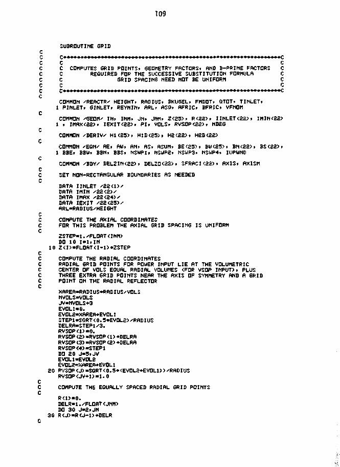
109
SUBROUTINE GRIDCC (;•*•***•**•»»»»>»»*»««»«»•«»»«»•**»»*»»*»••••»•••••••••••«»»«»»»»cc c cC C COMPUTES GRID POINTS* GEOMETRY FACTORS. AND B-PRIME FACTORS CC C REQUIRED FOR THE SUCCESSIVE SUBSTITUTION FORMULA CC C GRID SPACING NEED NOT BE UNIFORD CC C CC C«t««»>»«»««M«t«»«»«»««»«»>Hlt>MI« (M»»»««»t»«»«»»»MH««C
CCOMMON 'REACTR' HEIGHT* RADIUS. DKUGEL* FMDOT, QTOT. TINLET*1 PINLETt GIMLET, REYNIN* ftRlr «SQ» AFRIC* BFRIC* VFNOM
CCOMMON 'GEQrt' IN* INM. JN> JMM. Z<25>* R<2£>» IINLET<22>» IMIN(22>1 . IMAX(22>> IEXIT(22>* PI, VOLS, RVSQP<22>» NDEG
CCOMMON /DERIVE HI<23>» H1D<25>> H2<22). H2S<22>
CCOMMON 'EQN' REt fiW» AN* AS* ASUM> BE<25>« BW<25>» BN(22»> BS<22>>1 BBE* BEW. BBN> BBS. NSWP1, NSUP2* NSUP3* NSUP4» IUPUND
CCOMMON '-BDY/ DEL2IN<22)» DELZ0<22>* SFRACI<22>* AXIS* AXISM
CC SET NON-RECTANGULAR BOUNDARIES AS NEEDEDC
DATA I INLETDATA IM1NDATA MAX '82<S4>'DATA IEXJT ^22<25>^ARL«RADIUS'HEIGHT
CC CDMPUTE THE AXIAL COORDINATESC FDR THIS PROBLEM THE AXIAL GRID SPACING IS UNIFORMC
ZSTEP-1. /-FLOAT <INM>DO 10 IMiIN
10 Z<I>-FLOAT<I-1>»ZSTEPCC COMPUTE THE RADIAL COORDINATESC RADIAL GRID POINTS FOR POWER INPUT LIE AT THE VOLUMETRICC CENTER OF VOLS EQUAL RADIAL VOLUMES <FDR VSOP INPUT)* PLUSC THREE EXTRA GRID POINTS NEAR THE AXIS OF SYMMETRY AND A GRIDC POINT ON THE RADIAL REFLECTORC
XAREA-RADIUS+RADIUS'VOLSNVOLS-VOLSJV-NVDLS+3EVOL1«0.EVOL2-XAREA+EVOL1STEP1-SGRT <0.3«EV0L2> RADIUSDELRA-STEP1/-3.RVSOP<1>«0.RVSOP <S> «RVSOP <1>+DELRARVSOP <3>-RVSDP <2> +DELRARVSOP<4)«STEP1DQ 20 J-5.JVEV0L1-EV0L2
20 RVSOP <J>»SQRT<0.5*<EV0L2+EV0Ll>>'RADIUSRVSOP<JV+l>«1.0
CC COMPUTE THE EQUALLY SPACED RADIAL GRID POINTSC
R<l>*0.DELR-1.'FLOAT<JNM>DD 30 J»2*JN
30 R<J>«R<J-t>+DELR

170
C COMPUTE THE FflCTORS HEEDED FOR THE SP«TIfiL DERIVITIVESC
DO 40 I*2>INM
40DD SO J"2»JNMHa a>
SO H2D<J>»1.'<R<J*1>-R<J-1>>DO 60 J-1>JNU'lINUETCJ)
I4-IEXIT<J>DEU21N<J>«Z<I2>-2<I1)
60 DELZQ<J>«2<I4>-Za3>
CC COMPUTE THE B-PRIME FflCTORSC
00 70 I»2rINM
70DO SO J"2»JNMDR-0.S*H2D(J>
80C
RETURNEND
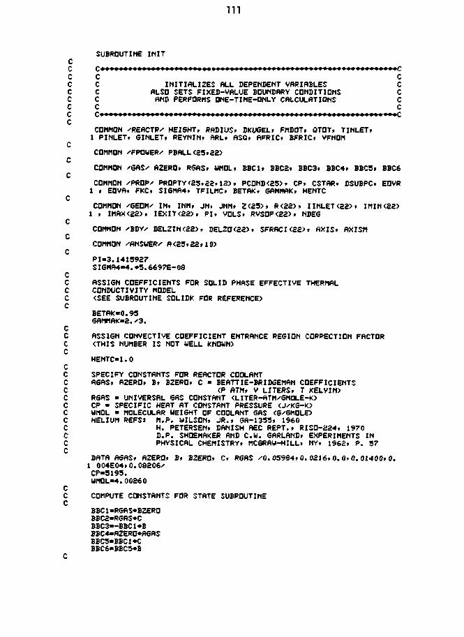
SUBROUTINE INITC
C C CC C INITIALIZES ALL DEPENDENT VARIABLES CC C ALSO SETS FIXED-VALUE BOUNDARY CONDITIONS CC C AND PERFORMS ONE-TIME-ONLY CALCULATIONS CC C CC C* ' «»»«MI»>MK«>«»«>«»»»»«t»t««»»>»«»t CC
COMMON 'REACTR' HEIGHT, RADIUS* DKUGEL, FMDDT, QTOT, TINLETf1 PINLET. GINLET, REYNIN, ftRL, ASQ, AFRICf BFRIC> VFNOM
CCOMMON 'FPOWER' PBALL (25,22)
CCOMMON 'SAS' AZERO. RGAS, WMOL, BBClt BBC2, BBC3» 8BC4, BBC3, BBC6
CCOMMON •PROP-' PR0PTY(25,2a,12), PCON0<25), CP> CSTAR, DSUBPC, EOVR1 » EOVA, FKC, SI6MA4f TFILMC, BETAK, GAMMAKf HENTC
CCOMMON 'GEOM' IN. INMi JN. JNM, 2<25>. R<22>. IIhLET<2£). IMIN<22>1 • IMAX(22>> IEXIT<22>> PI, VOLS> RVS0P<22>. NDEG
CCOMMON ^BDYx DELZIN<;22>, DELZ0<22>, SFRACI <22> • AXIS. AXISM
CCOMMON 'ANSWER' A<25.£2»10>
CPI-3.1413927SIGMA4-4.«5.6697E-08
CC ASSIGN COEFFICIENTS FOR SOLID PHASE EFFECTIVE THERMALC CONDUCTIVITY MODELC <SEE SUBROUTINE SOLID* FDR REFERENCE)C
BETAK-0.95GAMMAK»2.'3.
CC ASSIGN CONVECTIVE COEFFICIENT ENTRANCE REGION CORRECTION FACTORC (THIS NUMBER IS NOT WELL KNOWN)C
HENTC"1.0CC SPECIFY CONSTANTS FOR REACTOR COOLANTC A6AS; AZERO, B. BZERD, C > BEATTIE-BRIDGEMAN COEFFICIENTSC (P ATM, V LITERS, T KELVIN)C RGAS • UNIVERSAL GAS CONSTANT (LITER-ATM'GMOLE-K)C CP • SPECIFIC HEAT AT CONSTANT PRESSURE <J'KG-K>C UMOL • MOLECULAR WEIGHT OF COOLANT GAS (G'GMOLE)C HELIUM REFSi M.P. WILSON, JR., GA-1355, I960C H. PETERSEN, DANISH AEC REPT., RISO-224, 1970C D.P. SHOEMAKER AND C.W. GARLAND, EXPERIMENTS INC PHYSICAL CHEMISTRY, MCGRAW-HILL, NY, 1962, P. 57C
DATA AGAS, AZERO, B, BZERO, C, RGAS '0.05984,0.0216,0.0,0.01400,0.1 004E04,0.08206'CP-5195.WMDL-4.00260
CC COMPUTE CONSTANTS FDR STATE SUBROUTINEC
BBC1-RGA3*BZEROBBC2>RGAS«CBBC3—BBC1*BBBC4«AZERD«AGASBBC5»BBC1*CBBC6-BBCS«B

112
C CflLL SUBROUTINE TD CALCULATE INLET COOLANT DENSITYC
PINATM-PINLET'l.013E05CfilLL STATE <PINATM>TINLET>RHOIN>
CC COMPUTE INLET PLENUM VALUES FOR SELECTED VARIABLESC SEE SUBROUTINE PROPS FDR REFERENCESC
FMUIN«3.674E-07*TINLET**0.7TEMP«TINLET**<Q.71»a.-eoE-09»PINLET>>FKIN«2.6S2E-03»a.-1.123E-08»PINLET>»TEMPFKC-l.^FKIN
CCOEFFl-S.^AFRIC<BFRIC*DKUSEL>C0EFF2"6. •BFRIC'DKUGELHTODK-HEIGHT/'DKUSELTFILMC-TINLET*0.3
CG2 NLET-FMOOT' <RAD IUS«*ADI US*P I >REVNI l i -61 NLET»DKUGEL'FMU INVCG« <1.-VFNOM> ^VFN0M*«3Gl IN»36. •AFRIC^FMUIN* <1 . -VFNOM) *VCG' <RHOIN*DKUGEL*DKUGEL>G2IN»C0EFF2*VCG^RH0INCSTflR«CP*GINLET««EIGHT»FKC
CC ftSSUME PLUG FLOW FOR STREAM FUNCTION INITIAL GUESSC
00 10 J*2»JNI1IL-IINLET<J>IH»IEXIT<J>DO 10 I - I L » I H
10 fl<I»Jfl>»R<J>*fi<J)«0.5CC THE INLET COOLRNT PRESSURE IS SPECIFIEDC INITIAL GUESS FOR PRESSURE CORRESPONDS TO A DNE-DIMENSIONALC UNIFDRM PRESSURE DROP. ASSUMING THE OVERALL CORE DELTA P ISC 190 PERCENT OF THAT CALCULATED USING INLET CONDITIONSC
PERCNT-1.90CDELP-PERCNT**? INLET* <G 11N+G21 N*G I NLET> *HE IGHTDO 20 J-l-JNIL"IMIN<J)IH»IEXIT<J>DO 20 I«IL»IH
20 A<I»J>4>«<PINLET-CDELP*Z<I))''PINLETDSUBPC-GINLET^GINLET*G2IN*HEIGHT'PINLET
CC ASSIGN APPROXIMATE DISTRIBUTION OF PEBBLE THERMAL CONDUCTIVITYC CONSISTENT WITH THE AXIAL GRID SPACINGC PEBBLE THERMAL CONDUCTIVITY IS A FUNCTION OF FAST NEUTRONC FLUENCE AND TEMPERATUREC THE THERMAL CONDUCTIVITY OF THE FUELED MATRIX AND UNFUELEDC SHELL ARE ASSUMED EQUALC THIS DISTRIBUTION CORRESPONDS TO AN IDEALIZED OTTO FUEL CYCLEC REF: JUL-1114-RGJ 1974» FiS. 23» P. 63C
DO 30 I-l.IN30 PCONO <I> -17. +20.5»EXP (-15.37^2 <I> >
CC ASSIGN CONSTANT VALUES OF RADIAL AND AXIAL TURBULENTC PECLET NUMBERSC COMPUTE RATIO OF TURBULENT THERMAL DIFFUSIVITY DIVIDED BYC AXIAL VELOCITYC REFS: B. FINLAYSDN» CHEM. ENG. SCI.J 26. 1971 * P. 1081C H. DEANS AND L. LAPIDUS; AICHE J.» 6> I960* P. 656C
PECLTR»10.EOVR-DKUGEL/-PECLTRPECLTA-2.EOVA-DKUGEL'PECLTA

113
C SET THE BED VOID FRftCTION DISTRIBUTIONC FDR KFfl DESIGNS THE ENTIRE BED CfiN BE RSSIGNED THE NOMINflLC VflLUE DF 0.39C
DO 40 J«1»JNIL«IINLET<J> •
DO 40 I - I L , I H40 PROPTYa>J»4>*VFN0M
C CfiLCULflTE THE NDN-DIMENSIONfiL SPECIFIC SURFACEC
DD 50 J*1>JNIL*IINLET<J>1H»IEXIT<J>DO 50 I*IL»IH
50 PROPTY<I3J»5>• <1.-PRDPTY<I»J»CC flSSISN KW'BflLL DfiTft TD EXTRft GRID POINTS NOT USED BY VSOPC
DO 60 J - l » 3IL«IIHLETCJ>
DO 60 I - I L J I H60 PBRLL<IfJ>«PBRLL<I>4)
IL»IINLET<JN>IH«IEXIT<JN)DO 70 I«IL»IH
70 PBfiLL(I>JN>»PBfiLL<I»JNM>CC CflLCULflTE TOTflL POWER IN WflTTS FROM VSOP INPUTC
QTOT«0.VBALL*PI•DKUGEL*DKUGEL*DKUGEL^6.DO 30 J*4»JNMIL«IMIN<J)
DO 30 I - I L . I HO«PBfiLL <11J)•< X.-PROPTY <I» J» 4> >^VBftLL
SO OTOT-OTOT+O1)0 90 J-4.JNM1*1 INLET <J>Q*0.5*PBfiLL <I» J>•<1.-PROPTY <I» J > 4>)•VBflLLQTOT-QTOT+QI-IEXIT<J>Q«0.5*PBftLL <I»J> • <1. -PROPTY <I»J» 4> > •VBflLL
90 QTOT-QTOT+QPVOL-VOL S*FLOflT <INM>QTOT«OTOT*1.E03*HEISHT»RflDIUS»RflDIU
CC CfiLL ROUTINE TD INTERPOLRTE VSOP THERMflL POWER PROFILEC TO EVENLY SPftCEB RftDIflL GRID POINTSC
Cfi-LL INTERPCC SET STREWI FUNCTION RflDIHL BQUNDHRY CONDITIONSC
IL-IINLET<1>IH-IEXIK1)DO 100 I-IL-IH
100 R<I>l.l>*0.uIL«IINLET(JN>IH«IEXIT<JN>DO 110 I*IL»IH
110 ft<I»JN»l)»0.5CC SET BOUNDflRY CONDITION ON PRESSURE ftT INLETC
DO 120 J=1»JNI«I INLET <j:>
120 fH<l!.J»4>»1.

114
C INITIALIZE MASS-FLUX DISTRIBUTIONC
SO 130 J»2.JNIL-IINLET CJ>IH-IEXITO,SO 130 I - IL . IHCALL MFLUX <I.J>
130 CONTINUEIL"IINLET<1>IH-IEXIT<1>00 140 I-IL.IHCALL MFLUXXUlX
140 CONTINUE
C CALCULATE CONSTANT FACTORS DEPENDENT ON INLET CONDITIONS.C GEOMETRY AND VOID FRACTION DISTRIBUTION
DO 150 J - f t jN"SFRAC I <J> • 1 . -PROPTY < 1»J . 4>IL-IINLET<J)IH-IEXIT<J>DO 150 I»XL»IH5FRAC-1.-PROPTY <I» J» 4)RflTIO"SFRftC/'PROPTY <I t J» 4> • • SPROPTY <I>J»6>"SFRftC^COEFF1•GINLET
150 PROPTY<I»J»7>»C0EFF2*RftTI0^GaiN
C CONVERT KM^BfilLL DflTfl TO W'BflLL fiND D1MENSIONLESS VOLUMETRICC GENERATION RATE* QSTfiRC CALCULATE INITIAL GUESS FOR COOLANT BULK TEMPERATUREC BASED ON ENTHALPY RISEC TEMPORARILY SET TSURFACE«TGASC
DELTZ"HEIGmVFLOAT <INM>GCPI«1.s<SINLET«CP>P1«HEIGHT*HEIGHT«FKCDO 160 J«1»JNTFM-1.IL-IINLET<J>IH»IEXIT<J>BD 160 I»IL»IHPBALL<I»J>«l.E03*PBALL<I»J>CtT-PBALL <I»J> • <1. -PROPTY < I r J» 4> > • <VBALL*TINLET>VOLCOR-1.0IF <a.EQ. IL>.OR. <I.EO. IH>) VOLCOR«0.5A <I,J»£>«QT*VOLCOR»DELTZ*GCP1*TFMTFM«A<l»J»e>
160 PROPTY<I»J»S>>»QT*P1c • ' • • . • • •
C INITIALIZE BED AND COOLANT PROPERTIES <INCLUDING THE CQNVECTIVEC HEAT TRANSFER COEFFICIENT FOR THE NEXT STEP>C • • • '
CALL PROPSCC CALCULATE INITIAL GUESS FOR AVERAGE PEBBLE SURFACE TEMPERATUREC ASSUME 100 PERCENT OF THE HEAT TRANSFER IS BY CONVECTION
c ':PERCNT«1.0DO 170 J«1»JNMIL-IINLETCJ)IH-IEXIT<J>DO 170 I«IL>IHTDRDP-RROPTY < I . J» 9> > <P(?DPTY XI»J. 8> *PROPTY < I , J, 5) >
170 A<I»J»3>*PERCNT»TDROP+A<I»J!>2>IL»I INLET <JN.>IH»IEXIT<JN>DO 130 I-IL>IH
130C •
RETURNEND
115
SUBROUTINE STATE <P»T»RHO>
C C , CC C SOLVES THE BEATTIE-BRIDGEMAN EQUATION OF STATE CC C USIN6 NEWTONS METHOD CC C CC C REPi APPLIES NUMERICAL METHODS' CC C 8. CARNAHAN* H.A. LUTHER AND J.O. UILKESr CC C JOHN UILEY AND SONS* NY; 1964» P. 173 CC C CC c* ************* »«I»»»»>»<»»»»»»MHIO»»»»»«»»»>M»»I »>««»•>» >»>«Cc
COMMON 'GAS' AZERO> R6AS> UMOLt BBC1. BBC2> BBC3. BBC4, BBC5. BBC6C
TSQ-T»TBETA-BBC1*T-AZERO-BBCa^TSQGAMMA-BBC3*T4-BBC4-BBC5'TSG!DELTA-BBC6/TS0
CC USE IDEAL 6AS LAW FOR FIRST GUESSC
CC BE6IN NEWTONS METHOD ITERATION ON VC
DO 10 1-1.20DELTAV* < < < < <-P«V+RGAS*T> •V+BETA)»V*SAMMA>•V+DELTA> *V>•< < <RGAS*T*V*1 2 B E T A > V 3 e A AV-V+DELTAVIF <ABS<DELTAV/'V>.GT. l .E-06> GO TO 10GO TO 20
10 CONTINUECC RECOVER DENSITY FROM MDLAR VOLUMEC
20 RHQ-UMOL'VC
RETURNEND

116
SUBROUTINE INTERPCC C«>»«»»*>»»»»<»'<'«»«»*»«»»«»'»>>«>» »»>>«»««»»«»>»»» cc c cC C INTERPOLATES POWER PER BALL DATA PROM VSQP EQUAL-VOLUME CC C RADIAL 6RID POINTS TO EQUALLY SPACED RADIAL GRID POINTS CC C USING NEUTONS DIVIDES-DIFFERENCE INTERPOLATING POLYNOMIAL CC C CC C REFi APPLIED NUMERICAL METHODS* CC C B. CARNflHAN* H.A. LUTHER AND J.O.WILKESf CC C JOHN WILEY AND SONS* NY* 1964* PP. 17-26 CC C CC £•»»•»»*»»**•*»»»»»»»*»»»»»*«»»*»••«»*»**»**»*»»»»»»»**»*»*»•»»»*C
cCOMMON 'FPOUER' PBALL«5.22>
CCOMMON 'SEOM' IN* INN* JN» JNM* Z<23>» R<22)» I INLET(22 ) . IMIN<23>
1 * IMAX(22>f IEXIT<22>» P I * VOLS* RVS0P<22>* NDE6C
DIMENSION P<22>, TftBLE(22»2a>C
DO 30 1*1»INDO 10 J«1*JN
10 P<J>»PBALL<I»J>CALL DTABLE <RVS0P*P*TA8LE*JN*M*TRUBL*22>IF CTRUBL.EO.O.J 60 TO 20PRINT 40RETURN
20 DO 30 J*1*JNRARS>R<J>
30 PBALL<I*J>"FNEWT<RVS0P*P*TABLE*JN*M*NDE6>RARS>TRUBL*22>RETURN
C40 FORMAT <y»SX»•ARGUMENT ERROR IN INTERP CALL TO DTABLE OR FNEWT*)
END
117
SUBROUTINE DTftBLE <X»Y»TABLEfN»M»TRUBL»K>CC C***»»>>***»«*»»» »»»«»»»»>»»»»»»»»«»»«»»»«»»»»i»»»>»»»«««CC C CC C SUBROUTINE REQUIRED BY SUBROUTINE INTERP CC C CC C«»i>i»»i>>»<»»«>»»»»mnt«>»»»>M»»«>n>»n»«»n«»»n*»*»i»CC
DIMENSION X<N>» Y<N>, TABLE<K,K>
IF <M.LT.N> 60 TO 10TRUBL'1.0RETURN
10 NM1-N-1DO 20 1*1 tNM
20 TABLE<I»1>»<Y<H«!>-Y<I>>'<X<I+1>-X<I>>IF <M.LE. 1> GO TO 40DO 30 J-2.MDO 30 I-J.NfllISUB-H-1-J
30 TABLE<I»J>»<TflBLE<I»J-l>-TABLEa-l>J-l>>'<X<I+l>-X<ISUB>>40 TRUBL-0.
RETURNENDFUNCTION FNEWT <X»Y.TABLE»N»M.NDEG»XftRG»TRUBL»K>
CC C»«»>>*««*«»»«»««»»»*«»>««»»»»«•«»««•»»»«»»«»»>«»»>>>*»>»>>>»*»>>Cc c cC C FUNCTION REQUIRED BY SUBROUTINE INTERP CC C CC C ».I»>«M1 .«»«»»«>«»>»»«>»»«»•« I»»>MM»»CC
DIMENSION X<N>» Y<N>» TftBLE<K»K>C
IF <NDEG.LE.M> GO TO 10TRUBL»l,0FNEWT«0.RETURN
10 DO 20 I - l . NIF <I.EQ.N.QR.XAR6.LE.X<I>> GO TO 30
20 CONTINUE30 MAX'I+NDEG'2
IF <MAX.LE.NDEG> MBX-NDEG*1I F <MftX.GT.N> MftX-NYEST-TABLE <MAX-1» NDEG)IF <NDEG.LE.1> GO TO 50NDE6M1*NDEG-1DO 40 I-lfNDEGMlISUBI-MAX-1ISUB2-HDEG-1
40 YEST«YEST*<XARG-X<ISUBl>>*TftBLE<ISUBl-l»ISUB?>50 ISUB1«MAX-NDEG
TRUBL«0.FNE»T»YEST*<XARG-X <ISUB1>>•Y<ISUB1>RETURNEND

118
SUBROUTINE PROPS
C c**»******************************»•••»»««»»>«»»««»«»>*»««••>*>>«C
c c cC C COMPUTES PROPERTIES DF COOLANT AND RANDOM PACKED SPHERE BED C
c c cc c»»*»««»»»»»>««•••»•»»•«••••«•»«»» >•*«•«>i«»»»««»»«>«««««««««»»c
cCOMMON 'REACTP' HEIGHT. RADIUS. DKUGELi FMDOT. OTOT» TINLET>1 PINLET. GINLET. REYNIN. ARLt ASQ. AFRIC. BFRIC» VFNOM
CCOMMON •PROP/' PR0PTY<23.22>12>» PC0ND<23>» CPt CSTRR» DSUBPCi EOVR1 » EOVA. FKCt SIGMA4. TFILMC. BETftK. GAMMAKt HENTC
CC3MM0N •6EDM/' Ili. I MM. JN« JNM> 2<23>. R<22>> 11NLET <22>. IMIN<22>1 t IMFiX(22>» IEXIT(22>> Pit VDLS. RVSDP<22>» NDE6
CCOMMON 'ANSUER' fl<23>22«10>
CC PflRTS DF THIS ROUTINE flRE ONLY VRLID FOR HELIUM COOLflNTC CDRRELftTIDMS USED IN THIS ROUTINE RPE FOR HIGH REYNOLDSC NUMBER FLOWSC
DO 20 J - 1 F J NIL«IINLET<J>IH-IEXIT<J>DO 20 I«IL»IH
CC flVOID PROPERTY UPDftTE FOR UNRERSONflBLE VftLUES OF THEC DEPENDENT VARIABLESC
IF <ft<I»J»4>.GT.0.93> 6D TO 10PRINT 30» fl(I»J»4>»I,JSO TO 20
10 IF <<ft<I»J»2>.LT.l.).0R.<ft<I»J.3>.LT.l.)> GO TO SOP«ft<l»J»4>*PINLETTFILM»<R<I,J.2>*ft<ItJ»3>>»TFILMCTBULK-R <J» J» 2>*TINLETTS»ft<I»J»3>'»TINLET
CC SOLVE BEflTTIE-BRIDGEMflN EQUATION OF STRTE FOR DENSITYC
CflLL STRTE <PRTM»TFILM»PROPTY<I»J.l>>CC COMPUTE CODLRNT <HELIUM> DYNftMIC VISCOSITY RND MOLECULRRC THERMftL CONDUCTIVITYC REFi H. PETERSEN. DflNISH REC REPT. RISO-224. 1970C
FMU»3.674E-07»TFILM»*0.7TEMP«TFILM»*<0.71-l.42E-09»P>FK-2.682E-O3*<1.+1.123E-08*P)*TEMP
CC COMPUTE EFFECTIVE THERMAL CONDUCTIVITY OF THE SOLID PHASEC
CRLL SDLIDK <I»J»TS>FK>SKE>PROPTY <1.J»10>»SKE*FKC
CC COMPUTE FRICTION PARAMETERSC
PROPTY<IfJ»2)•PR0PTY<I»J»6>*FMUPROPTY<I»J»3>»PR0PTY<I»J.7>^PRDPTY<IfJp1)

119
C COMPUTE EFFECTIVE THERMAL CONDUCTIVITY OF THE FLUID PHASEC REFSi E. SINGER AND R. UILHELM. CHEM. ENS. PROS.» 46»C 195O» P. 343C B. FINLHYSONt CHEM. ENS. SCI.r 26. 1971» P. 1031C
VOIDKF-PRQPTY <I ,J » 4>*FKRHOCP-PRDPTY(IfJ,l>*CPVC0N«6INLEVPR0PTY<I» Jt 1>
ETURBR-EOVR«AVELETURBft-EOVfHflVELPROPTY <I»J » J1>•<VOIDKF+RHOCP*ETURBR> *FKCPROPTY <11J »12)-<VOIDKF*RHOCP«ETURBft>•FKC
CC COMPUTE THE CONVECTIVE HEftT TRANSFER COEFFICIENTC REFl H. BflRTMELSr BRENNSTOFF-UfiRME-KRflFT» 24. 1972C
REYNH-REYN^PRQPTY<I» J14>COEFF»<l.-PROPTY<I»J»4>>yPROPTY<IfJ,4>H» <2.0+ <COEFF*REYNM)••«.5+0.0 05*PEYNM> *FK^DKU6EUIF <I.EO.1> H*HENTC«H
20 PROPTY<I»J»8>«H«HEIGHT«FKCRETURN
30 FORMAT </»2X»•UNREASONABLE PRESSURE CALCULATED. A<I»J»4> » *>F6.4,1 3X»END

120
SUBROUTINE SOLIDK <ItJ.TS.FK,SKE>CCC C CC C CfU.CUL.ATE5 EFFECTIVE THERMAL CONDUCTIVITY CC C OF THE SOLID PHASE CC C CC C REFx D. KUNNI AND J.M. SMITH. AICHE J . . 6» I960* P. 71 CC C CC C»»»»«««»'»»»»»« »»»»«»»«»»» »«>«««««««««»»»>»»««>C
cCOMMON 'REACTft' HEI6HT* RADIUS. DKUGEL* FMDOT. QTQT. TINLET.1 PINLET» GINLET. REYNIN» ARLf ASQ» AFRIC* BFRIC» VFNOH
CCOMMON /PROP/- PR0PTY<23.22.12). PCOND<25>> CP. CSTAR. DSUBPC. EOVR1 » EOVA. FKCt SIGMA4. TFILMC. BETAK. GftMMftK. HENTC
CC COMPUTE PEBBLE THERMAL EMISSIVITYC ASSUMES 6RAPHITE EMISSIVITY CHANGE IS LINEAR WITH TEMPERATUREC REF* WELTYf J.R.» ENGINEERING HEAT TRANSFERC JOHN WILEY AND SONS. N.Y.. 1974C
TCUBE«TS*TS*TSRATID>DKUGEL./FKPART1-SIGMA4*TCUBEPARTa-PR0PTY<I»Jt4>/<2.*<l.-PROPTY<I»J»4>>>
HRS-PARTl«£MISS/'<2.-EMISS>RATIOK"FKxPCOND <I>
CC USE CURVE FIT OF PHII AND PHI2 DATAC
PHI1*0.2770«RAT!0K*»0.2426PHI2-0. 1293*R*TIOK~0.3292PHI"PHI2+<PHIt-PHI2)*<:PR0PTY<I.J»4>-0.£6> ^0.IF <PROPTY<I»J»4>.LE.0.26> PHI-PHI2IF <PROPTY<I.J.4>.SE.0.476> PHI-PHI1
PARTK1«PROPTY<I»J»4)*<1.PARTK2"!.•PHI t*ATIO*HRSPARTK3«BETAK*< 1i-PROPTY<I.J»4>>•<1.'PARTK2+6AMMAK+RATIOK>SKE"FK*<PARTK1+PARTK3>RETURNEND

121
SUBROUTINE MFLUX <I.J>
c c*»«»»«•»»«««»«»«<»»««»»»««»»»»«»«*«*»>»*•*»•»»«»»*»»»»»»•**»*»»*cc c cC C COMPUTES STREAM FUNCTION DERIVITIVES AND RECOVERS CC C THE MHSS FLUX. GSTAR. AND ITS COMPONENTS CC C ALSO APPLIES THE MD-SLIP CONDITION AT IMPERVIOUS BOUNDARIES Cc c cc c»»»*»«*»«»«»«*»•«»**•»**»••••••««««««««»««««»**»»»»»»*****»**«»»cc
COMMON •REACTR/' HEIGHT. RADIUS* DKUGEL. FMDOT. OTOT. TINLET.1 PINLET. GIMLET, REYNIN. ARL. ASQ. AFRIC. BFRIC. VFNQN
CCOMMON 'GEOM' IN. INM. JN. JNM. Z<25>? R<2S>> IINLET<22>» IMIN<22>1 • IMAX<S£>. IEXIT<22>. PI. VQLS. RVS0P<22>. NDE6
CCOMMON '8DY' SELZIN<22>. DELZ0<22>t SFRACK22). AXIS. AXISM
CCOMMON ^ANSWER/ A<25.22.10)
CC IF N0N-RECTAN(3ULAR BOUNDARIES ARE USED. EXPRESSIONSC EVALUATING DERIVITIVES AT THE BOUNDARIES MAY NEED TOC BE MODIFIEDC
INFACE-IINLET<J>I0UT»I6XIT<J>IF a.EQ.INFACE.QR.I.EQ.IOUT.OR.J.EQ.l.OR.J.EO.JN> GO TO 10A <I»J. 3> "DBYDZ <I» J» 1>A<I.J,7>«DBYDR<I.J.1)60 TO 30
10 IF a.NE.INFACE) GO TO 20
IF U.EQ.U GO TO 50IF <J.EG.JN> GO TO 60A<I.J»7>»DBYDR<I»J.1>GO TO 80
20 IF <I.NE.IOUT> GO TO 30
IF (J.EQ.1> GO TO 50IF CJ.EQ.JN) GO TO 60A(I.J.7>-DBYDR(I.J.1>GO TO 30
30 IF CJ.NE.JN) GO TO 40GO TO 60
4ft A<I.J.3>-0.050 A<I»J»7>*<A<I»2.1>-A<I.
GO TO 70CC TREATMENT OF GSTAR ALONG THE IMPERVIOUS RADIAL WALLC APPLY THE NO-SLIP CONDITION AT ALL IMPERVIOUS BOUNDARIES?C I.E. GZSTAR»GRSTAR«G3TAR»0C
60 A(I»J.7)-0.0A<I.J»8><*0. 0A(I>J>9)-0.0A<I.J.10>«0.0A<I.J.5>-0.0GO TO 100
CC TREATMENT OF GZSTRR ALONG THE AXIS OF SYMMETRYC
70 A<I»J.10>»0.0A<I.1.9>-AXIS»A<I»2,a>-AXISM*A<I,3.9>GO TO 90
80 A<I»J»9>»A<I»J.7>^R<J>A <I > J > 10>—ARL^A < I, J»8>'R < J>A<I»J»5>«SQRT<ASQ*A<I»J»8)*A<I»J.3>+A<:i>J.7>»A<I.J.7>>''R<J>GO TO 100
90 A<I.J.5>-A<I.J.9>100 CONTINUE
RETURNEND

333
OIT'I)
(33>3H C£3> IH
<>t»r *i>« Awatw 3Hi JDSIHIDd KDIdaiNX IV SAUIAIdSd
aws
MDUUD3
HDWWCID
00090****-
siwiDd aoia3xwiAttaaH 3Hi. do x 3ia«iaHA dD1H 3AUI(Mil3a 1«IX« XSI S3XndU03
,»»»»».»o3333
WDU3Kirid
WDWW03
M0MU03
da1ST S3indU03
»30333
D3333333
333333
<XT«I>
123
SUBROUTINE PDECC c»*»«»»»«««***»•»•••»»»»»«*«•»**»•>*****»**»•••»*«*«*»»•***»> >**<Cc c cC C CONTROL ROUTINE - EQUATION SOLVER FOR CC C ELLIPTIC PARTIAL DIFFERENTIAL EQUATIONS IN STANDARD FORM CC C CC C REFJ HEAT AND MASS TRANSFER IN RECIRCULATING FLOWS» CC C A.D. 60SMAN» W.M. PUN. fl.K. RUNCHAL, CC C D.B. SPALSIN6 AND M. UOLFSHTEIN* CC C ACADEMIC PRESS. LONDON. 1969 CC C CMODIFIED HEREIN) CC C Cc c««»*««>»»»*»*»»»»*»»»*»««*««»»»»»»»»«»»»*«»««>»««»«*»««»«»»»»»«»cc
COMMON •PROP' PR0PTY<25.2fi»t2>» PC0N0<£5>» CP* CSTAR* DSUSPC* EOVR1 . EOVA. FKC. SIGMA4. TFILMC. BETAK. GAMMAK. HENTC
CCOMMON /-GEDM/- I N . INM. Jti, JNM. Z<29>> R(22>. I INLET<22) . IMIN<22>
1 . IMAX<22>. IEXIT<22>» P I , VDLS. RVS0P<22>» NDEGC
COMMON -'NUMERr RP<4>. RSDU(4>. LOC!(4)> LOCJ<4>. REDUCE* IOVERC
COMMON 'EQN' AE> AW, AN, AS, ASUM, BE<25>» SU<25>, BN<22>, BS<22>,1 BBE. BBU, BBN, BBS, NSUP1, NSWP2, NSUP3, NSUP4, IUPUND
CCOMMON •ANSWER' A (25 .22 .10 )
CC STREAM FUNCTION SUBCYCLEC
00 20 N-1,NSWP1RSDUCD-0.90 10 J«2,JNM
IH»IMAX<J>DO 10 I>IL,IHIM-I-1IP-I+1JM-J-1JP-J+1CALL MFLUX <I»J>CALL MFLUX <IP,J)CALL MFLUX <IM,J)CALL MFLUX <I,JP>CALL MFLUX <I,JM>A<I»J,6>-<A<I.J»5>+PR0PTY<I,J.2)>*PR0PTY<I,J,3>A<IP»J,6)-(A<IP,J,5)+PR0PTYaP,J,2>>*PR0PTYaP,J,3>A<IR,J,6>«<:Af.IM,J,5>*PR0PTY<:iM,J,2))*PR0PTY<IM,J,3>A<I,JP,6>-<A<I,JP.5>+PR0PTY<I.JP,2>>*PR0PTY<I,JP!.3>IF <J.EG.JNM> A<I,JP,6)>A<I,J,6>A<I,JM,6>»<A<I,JM,5>+PR0PTY<I.JM,2>)*PR0PTY<I»JM,3>BPP«A<I,J,6>BBE"<A<IP,J,6>+BPP»*BE<I>
BBN- <A < I , JP, 6> +BPP> •BN < J>BBS* CA < I , JM, 6> +BPP) •BS < J>
CC CALL EQUATION SOLVER ROUTINEC
10 CALL SOLVE CI.J.l)CC ITERATE ON BOUNDARY CONDITIONSC
CALL BOUND1C
20 CONTINUEC

124
C FLUID BULK TEMPERATURE SUBCYCLEC
DO 40 N-1.NSUP2RSDU<2>«0.00 30 J«2fJNMIL-IMIN<J>IH-IMAX<J>DD 30 I«IL»IHBPR»PROPTY<I»J.11>BPA-PROPTY < I * J > 12)BBE- <PROPTY <I+1 > J» 12) +BPft> *BE <I)BBU« <PRDPTY < I - l»J» 12)+BPft>*BW <I)BBN-<PROPTY<I»J*1» it>+BPR)*FM<J)BBS»<PROPTY<I.J-1»U>*BPR)*BS<J>
CC CALL ROUTINE TO CALCULATE fiE. AM. AN> AS AND ASUMC
CALL ADVEC <IFJ>CSTAR>C
30 CALL SOLVE <I»J»2)C
CALL BOUNDSC
40 CONTINUECC AVERR6E PEBBLE SURFACE TEMPERATURE SUBCYCLEC
SO 60 W-1.NSWP3RSDU<3>»0.DO 90 J-2.JNMIL-IHIN<J>IH-II1AX<J>SO 50 I«IL»IHBPP»PROPTY<I.J»10>BBE-<PROPTY <I+l»J»10>+BPP>*BE<I)BBU»<PRaPTY<I-l»J»10)+BPP>*BU<l)BBN« <PROPTY < I. J+1»10) +BPP) *BN < J)BBS*(PROPTY <I»J-lf10> +BPP> »BS <J>
C50 CALL SOLVE <I»J»3>
CCALL B0UNS3
C60 CONTINUE
CC PRESSURE RECOVERY SUBCYCLE
DO SO t1*lft1$UP4RSDU<4>>0.DO 70 J-2.JNM
IH>IMAX<J>DO 70 I« IL i IHBBE«2.*BE<D
BBN»2.*BN<J)BBS*2.«BS<J)
C70 CALL SOLVE <I»J»4)
CCALL B0UN04
C80 CONTINUE
CC UPDATE PROPERTIES BASED DN NEW VALUES OF THE DEPENDENTC VARIABLESC
CALL PROPSC
RETURNEND

725
SUBROUTINE SOLVE <l,J,K>CC (;>»*»••>••••<
c c cC C COMPUTES NEW VALUE OF VARIABLE FKI.J.K) CC C THROUGH APPLICATION OF GENERAL SUBSTITUTION FORMULA CC C Cc c»»«*«»«••«»*»»*»««»»»*«»«»«»»**»»»*»*»»»»»»»«»»»«»«»*«»«»»»»»**«cc
COMMON •NUMER' RP<4>» RSDU<4)» L0CI<4>» L0CJC4). REDUCE. IOVERC
COMMON 'EON' AE> AW. AN. AS» ASUMt BE<25>» BU<S5>» BN<22>. BS<22>»1 BBE. BBW. BBN. BBS* NSWP1, NSWP2. NSWP3. NSWP4. IUPWND
CCOMMON /ANSWER' ft <25.22.10)
CC CALCULATE THE VALUE OF D-SUBPHIC
CALL DTERM U.J.K.DPHI)
ADNM>ASUM+BBE+BBW+BBN+BBSIF <ADNM.EO.O.> 60 TO 30
CC STORE THE OLD VALUE OF THE DEPENDENT VARIABLE KC
CC CALCULATE THE NEW VALUEC
IF <<K.EQ.1>.OR.<K.EQ.4>> GO TO 10CC OVERRIDE NORMAL SUBSTITUTION FOR TEMPERATURES IF STABILITYC COULD BE A PROBLEMC
IF <ANEW.6T.1.0> GO TO 10ft < I . J . K> »REIiUCE*OLDIF <IOVER.EQ.1> PRINT 40. I.J.K.OLD.ANEW.A<I»J»K>GO TO SO
CC UNDER OR OVER RELAX IF SPECIFIEDC
10 A<I»J.K>-OLD+RP<IO* (ANEW-OLD)CC CALCULATE THE RESIDUALC
SO RS-l.-OLD'AHEWCC STORE THE MAXIMUM RESIDUAL AND ITS LOCATIONC
IF (ABS(RS>.LE.ABS<RSDU<K)>> GO TO 30RSDUOO-RSLDCIOO- ILQCJOO-J
30 CONTINUERETURN
C40 FORMAT <^»2X.*N0RMAL SUBSTITUTION OVERRIDDEN FOR STABILITV^»/'»3X»*
II > •.12.*. J « •,I2»». K • •.II.*. OLD - •.F6.3.*. NEW • •fF?.3,*2. fl<I.J.K> • *»F6.3>END

126
SUBROUTINE ADVEC CI.J,APP>C
C C CC C COMPUTES ADVECTION TERMS OF GENERAL SUBSTITUTION FDRHULA CC C Cc c»»*»**»»**»•»*>*»»»*»••»»»»»»»*»»»»«»»»>»««»»*>»»>«>»>»»«>»»»««»cc
COMMON sGEO»/ IN . INM. JN» JNMt Z<23>» R<22>» IINLET<22>t IMIN<22)1 • infix(S2>» IEXIT<22>. P I . VOLSt RVS0P<22>> NDE6
COMMON -'EON/- flE, flW, flM. flS. ftSUM. BE(2S)» BW<25>» BN<22). BS<22>.t1 BBE. BBW, SBN> BBS. NSUPlf NSUP2. NSUP3* NSWP4. IUPWND
CCOMMON ^RNSUER'' fl<"25»22»10)
C
GRPS»Cft<I-l»J,l>-f l<I+lf J t l > - f A < I - l , J -GRPN»<fl<I-l»J. l)-ft<I*l»J»l)*ft<I-l,J+
CC COMPUTE ftE> FIW» ANt AND ASCC USER HAS OPTION OF USING UPWIND OR CENTRAL DIFFERENCESC CENTRAL DIFFERENCES ARE MORE ACCURATE* BUT UPWINDC DIFFERENCES NAY BE REQUIRED TO ENSURE CONVERGENCEC
IF (IUPUND.NE.1> GO TO 10CC UPWIND DIFFERENCESC
AE-0.3*APP* <ABS <GZPE>-GZPE>AUI-0.5»APP*<ABS <G2PW> •GZPW)AN»0. 3*ftPP» <ABS <GRPN> -GRPN>AS»0.
RETURNC
10 CONTINUECC CENTRAL DIFFERENCESC
AE«-0.5*flPP»GZPEAW"0.5*APP*6ZPWAN"-0.5»APP*GRPNAS»0.5*APP*GRPSASUM— <AE+AW+AN+AS)RETURNEND
127
SUBROUTINE BTERM <I»J»K»DPH1>CC C«C C CC C COMPUTES D-SUBPHI TERM OF STANDARD ELLIPTIC FORM CC C CC C** «,»»»»».»••»»»»»»»» ««»•».» »»»»».««CC
COMMON 'REACTRx HEIGHT. RADIUS. DKUGEL» FMDOT. G 3T. TINLETft PINLET. SINLET. REYNIN. ARL» ASQ. AFSIC* BFRIC> VFNOM
CCOMMON 'PROP' PRQPTY<23t22rl2>> PC0ND<25>» CP» CSTAR» DSUBPC* EOVRI t EOVA» FKC» Sl&HHr TFILMC. BETAK» «3ftMMftK» HENTC
COMMON sGEQns IN» INM» JN» JNMp 2<2S>> R<22>* IINLET<22>» IMIN<22>t > IMAX(22>» IEXIT<22>. P I . VDLS. RVS0P<22>» NOE6
CCOMMON /'ANSWER^ A<25»22.10>
CC SELECT THE TERN CORRESPONDING TO VARIABLE KC
GO TO a0.20»3O»4O>» KCC STREAM FUNCTION SUBCYCLEC
10 DPHI«2.»A(I.J.6)«A<I.J»7>/<ASQ»RU)>RETURN
CC FLUID BULK-TEMPERATURE SUBCYCLEC
20 DELTft«A<I»J»3>-A<I»J»2>DPHI--PROPTY <11J» 3>»PROPTY <I.J.8>•DELTFRETURN
CC PEBBLE AVERAGE SURFACE TEMPERATURE SUBCYCLEC
30 DELTA-A<I.J.3>-A<I»J.2>DPHI*PR0PTY<I fJ.5>«PR0PTY<I»Jf8>*DELTA-PR0PTY<I.J.9>RETURN
CC PRESSURE RECOVERY SUBCYCLEC
40 DBDZ"DBYDZ<I»J»6>DBDR«0BYDR<IrJ»6>A<I.J»8>*DBYDZa>J»l>A<I.J»7>«DBYDR<I»J»l>DPHI«-<A<I»J»7>*DBD2-A<I,J»8>»DBDR>*DSUBPC^R<J>RETURNENS

128
SUBROUTINE BOUND
c c cC C ITERATES BOUNDARY COMDITIONS WHICH INCLUDE THE NORMAL CC C DERIVITIVE DF THE DEPENDENT VARIABLE CC C AND THDSE WHICH REQUIRE UPDATED VALUES OF OTHER VARIABLES CC C CC C •••••• » * « •••—•« « >« « « »»••»> »>«««nt»»t»n>»»»>»»>«»»>«t»«»»>i»»CC
COMMON /PROP/ PRDPTY^B.aSf 12>» PCDND <23>» CP» CSTAP. DSUBPCf EOVPI t £OVA» FKCr ZlGn*4i TFILHCf BETflK» GfiMMftKj HENTC
CCOMMON ^SEDM^ INf INM. JN, JNM. 2<23>» R<22>» I1NLET(22>» IMIN<22>
1 . IMflK<22>» IEXIT<22>» Pl» VDLS. RVS0P<22)f NDEGC
COMMON /BOY' DEL2IN<22>« DEL20<22>» SFRftCI<22>» flXIS. ftXISMC
COMMON ftNSWER^ H<25»22.10)CC SET UP FOP. CONSTANT Z INLET FflCE AT Z«0C AND CONSTANT 2 OUTLET FACE AT 2-1
C CONDITIONS CORRESPOND TO SYMMETRY AT R-0 flND P-lC THE RADIAL P.EFLECTDR IS ASSUMED IMPERVIOUS AND ADIABATICCC IT IS ASSUMED THAT THERE IS A CONSTANT PRESSURE IN THE INLETC PLENUM WHICH LEADS TO GRSTAR<1NLET>«O WHICH MAKES THE AXIALC OERIVITIVE OF PSI ZEROC IT IS ASSUMED THAT FLOW AT THE OUTLET IS PURELY AXIAL* ANDC THAT PRESSURE AT THE OUTLET FACE CORRESPONDS TO AC ONE-DIMENSIONAL AXIAL DROP FROM THE LAST INTERNAL GRIDC POINT AND HAS A CONSTANT VALUE ACROSS THE OUTLET FACECC TEMPERATURE CONDITIONS AT THE INLET ARE DERIVED FROMC ONE-DIMENSIONAL THERMAL EMERGY BALANCESC TEMPERATURE CONDITIONS AT THE OUTLET REQUIRE THAT THEC 2ND AXIAL DERIVITIVES OF THE TEMPERATURES EQUAL ZEROCC STREAM FUNCTION AT INLET AND OUTLETC
ENTRY BOUND!DO 10 J«£»JNM
10 A<INJJ»l ) -ACINMtJ»CALL MFLUX <1>1>CALL MFLUX <1»JN>CALL MFLUX < I N . l )CALL MFLUX <IN.JN>
A<IN»1.6>-<A<IN»t.5>+PR0PTY<IN,A<IN>JN»6>"A<IN»JNM.6>RETURN
CC FLUID BULK TEMPERATURE AT R«0» R«l» INLET AND OUTLETC
ENTRY B0UND2DO 20 J«2»JNMDTFDZa<A<2»J»2>-A<l»J»2>>/'DEL2IN<J>
20 A<IN»J»2>«DEL20a>»DBYD2<INM»J»2>+A<INM»J»e>DO 30 I«1»IN
30 A<I>JN»2>*A<I»JNM>2)RETURN

129
C PEBBLE AVERAGE SURFACE TEMPERATURE AT R-Of P - l . INLET AND OUTLETC
ENTRY BOUND3DO 40 J-2»JNHDTSDZ-<A<2>J.3>-A<1»J»3)>^DELZINtJ>TI 1»PRDPTY<1. Jf 9) •SFR.ACI < J> 'PROPTYa t J» 5>
40 A<IN»J»3)-DEL2D<J)»DBYDZ<INI1t J.3> •A<INM»DO 30 I»1»IN
30 A<I» JN»RETURN
CC PPE3SUR" AT OUTLETf R«0 AND R-lC
ENTRY BOUND4JB-JNM-1A (INt JB»4> —DSUBPODELta (JB> •*<• IN. JB» 9) ft < IN» JB» 6> •ACINM, JBtA>DO 60 J-2.JNM
60 A(IN>JDO 70
70 A<I>JN»4>»A<I»JNM»4>RETURN
CEND

130
SUBROUTINE TEMPSCC C>»>»<i»»«»«»«K»« »>ir»i>i*»ti»i>»<>»>»»>««««»««K»>«»«»»»«C
c c cC C CALCULATES PEBBLE INTERNAL TEMPERATURES CC C AND TEMPERATURE GRADIENTS CC C FOR BOTH CONVENTIONAL AND SHELL FUEL'MODERATOR ELEMENTS CC C ALSO RE-DIMENSIONALIZES TEMPERATURES FOR OUTPUT CC C CC C»«»»*»**>*>*»**«*«»*««*»»*»**««»>»**»*«**»*»*»>»»»«»**»«>*>»>*»*CC
COMMON 'REACTR' HEIGHT. RADIUS* BKUGEL. FNDQT, QTDT, TINLET»1 PINLET. SIHLET* REYNIN, ARLr ASQt AFRICt BFRIC» VFNOM
CCOMMON 'FPOWER' P>ALL<8Sf23>
CCOMMON 'PROP' PR0PTV<23fa2»12>» PC0NB<a5>» CP. CSTAR, DSUBPCt EOVR1 • EOVAr FKCr SISMA4, TFILMC. BETAK> GAMMAKf HENTCCOMMON 'SEaif INr INM» JM, JNM» Z<2$> * 9<Z2>f IINLST<22>» !MIN<22>1 » IMAX<22>» IEXIT<22>> PI» VOLS» RVSDP<22>» NBE6
CCOMMON 'ANSWER' A<2Sf22>10>
CCOMMON 'BALL' TEMPIN<2S»S2»3>f IBALL> Kit R2
CC IT IS ASSUMED THAT THE THERMAL CONDUCTIVITY OF THE FUELEDC MATRIX AND THE UNFUELED GRAPHITE SHELL ARE EQUALC IT IS ASSUMED THAT THIS THERMAL CONDUCTIVITY VARIES AXIALLYC BECAUSE OF AXIAL CHANGES IN TEMPERATURE AND FAST FLUENCE
C THE THERMAL CONDUCTIVITY VALUES ARE ASSIGNED IN SUBROUTINEC INITt WHERE A REFERENCE IS GIVENC
IF <IBALL.NE.1> GO TO 20CC CONVENTIONAL BALLC
R3*0.9*0KU6EL
C2"Ci*<t.'R2-l.'R3>C3"-0.Ol^Cl'<R2*R2>
DO 10 J"1»JNIL«IINLET<J>IH«IEXIT(J>DO 10 I»IL>IHTS«A<lrJ*3>»TINLETA<I»J.3>»TS
QOVERK»PBALL <I»J>'PCOND <l>TEMPIN<I»J»1>"OOVERK^Ca+TSTEMPIN <I*Jt 2>«aOVERK*C3
10 TEMPIN<:i.J,3)-«0VERK*C4*TEMPIN<I»J.RETURN

131
cC SHELL BALLC
20 R3»0.3*9KU6EL
C4«O.5*<RS«R2-R1«R1>
C6--0.0l«CI'<R2*R2>C7«CI«C3*<C4-C5>DO 30 J"1»JNIL»IIMLET<J>1H«IEXIT<J>DO 30 I-IL.IHTS»ft<I»Jt3>*TIMLET
OaV£RK«f>BALL <I» J> /-PCDND < I )TEMPIN<I»J»1>-OQVERK*C2+TS
30RETURNEND

132
SUBROUTINE RESULTCC i>>>n»<>»»«»««»»«>C CC C ROUTINE FOR FILM AND PRINT OUTPUT CC C CC C PLOT ROUTINES f»RE INSTALLATION DEPENDENT CC C PRINT OUTPUT FORMRT IS FOR AN 80 CHARACTER PftSE WIDTH CC C IF JN.GT.22 PRINT OUTPUT FORMAT MILL NEED TO BE MODIFIED CC C C
COMMON 'REACTR' HEIGHT. RADIUS. DKUGEL. FMDOT. QTOT. TINLET,t PINLET. GIMLET, REYNIN. ARL. ASQ. AFRIC. BFRIC VFNOM
COMMON •FPOWER^ PBftLL'.£3»£S>
COMMON /-PROP' PR0PTY<:a3»22»12>f PC0ND<25>» CP» CSTftR* DSUBPC* EDVR1 , EOVft. FKC> SIGMA4> TFILMC> BETHKP GftMliflK. HENTC
COMMON /GEOM' I N . INM» JN» JNM. Z<25)» R<22>» IINLET<S2>. IMIN<22>1 » IM«X<22>. IEXIT<22>. P I . V0L3. RVS0P<22>. NDES
CCOMMON 'fiNSWER' fl<23.22»10>
CCOMMON 'BRLL' TEMPIN<2S»22.3>. IBOLL. Rl» RS
CCDMMON /-RESULT^ I0UTP<12>» IF ILMt . IF ILM2. IF ILM3. JLnCTP. ID .
1 INDEX. KOfl. NCC
DIMENSION QUTVflR<22»23>» ZC<21)C
DIMENSION IOK<10>. KFILM<3>» JPL0T<3>CC SCfiLE SELECTED VRRIftBLES FOR PRINTOUTC
DO 10 Jsl.JNDO 10 I-l.IN
10 PBflLL<I.J>-PBftLL<I.J)*l.E-03
PINLET«PINLET*l.E-06CC CHLCULfiTE OUTLET PLENUM MIXED MEflN GAS TEMPERATURE. CORE PRESSUREC DROP. flND COMPARE COOLANT TEMPERATURE RISE ACROSS CORE WITH THftTC PREDICTED BY THE FIRST LAW OF THERMODYNAMICSC
SUPITFO-0.RIN«0.JNMM»JNM-1DO 2.0 Ja
AREft«ROUT»ROUT-RIN*RINSUMTFO«SUMTFO+AREA«fl <IN.J,5> *#<IN.J.2)
20 RIN>ROUTAREA*1.-RIN*RINSUMTFO«SUMTFO+AREA«« <IN» JNM.3> *A <IN.JNM.2>TFOMM»SUMTFO*GINLET*RADIUS*RADIUS«f> I'FMDOTPOMM-A(IN.JNM.4> *PINLETDELTAT-QTQT/- <FMDOT«CP>FSTLAU»<TFOMM-TINLET-DELTAT> *100./DELTATPDROP-PINLET-POMM

133
C LOCftTE MftXIMUM flND MINIMUM VftLUES IN FIELD OF SELECTED VfiRIflBLESC
TFMIN-1000.TFMftX-0.TSMIN-100O.TSMftX»O.PWRMIN-10.
PMIN»1.0PMHX»1.0TMXMIN-2OOO.TMXMftX»O.GRftDMX'O.SO 110 J«1»JNDO 110 I-l.INIF <TEMPIN<I»J,3).GT.TMXMIM> GO TO 30TMXMIN"TEMPIN<I»J>3>
30 IF <TEMPIIia»J»3).LT.T(1XMflX> SO TO 40TMXMBX-TEMPIM <I,J13>ITMXM-IJTMXM«J
40 IF <ft<I»J»3>.LT.TSMftX) 60 TO 50TSMRX«fl(I»J»3>ITSMflX-IJTSMflX-J
30 I F <ft<I»J»3>.GT.TSt1IM> GO TO 60
60 IF <R<I»J»4).GT.PMIN> GO TO 70PIW1»ft<I>J>4)
70 I F <fl<I»J»2>.GT.TF(irN) GO TD 80
30 I F <PBflLL<I»J).LT.PWR(WX> GO TO 90PMRMflX«PBftLL<I»J>IPWRMX-IJPWRHX-J
90 IF (PBfH.L<I»J>.GT.PWRMIN> GO TO 100PMRHIM-PBftLL <ItJ>
100 IF <TEMPIM<I»J»2>.GT.GRflDMX> GO TO 110GRftDMX-TEMPIM<I,J,2>IGRRO-IJGRftD»J
110 CONTIflUEDO 120 J»1>JNIF tft<IN»J»2>.LE.TFMRX> GO TO 120TFMf>X»ft<INt Jf2>JHQT-J
120 CONTINUERHOTC«R<JHOT> *RRDIUSRMPWR-R<JPURMX)*RftDIUS2MF'JR-2<IPWRt1X> *HEIGHTRMFUEL-R <JTMXM)•RflDIUSZMFUEL«2 CITI1XM> •HEIGHTRTSMftX«R <JTSIWX> •RflDIUS2TSMHX-2 <ITSNflX)•HEIGHTRGRRD-R<JGRftD>•RflDIUSZGRAD«Z<IGRflD)•HEIGHTRTFMftX»R <JHOT>•RADIUS

134
C OUTPUT INLET PLENUM VALUES AND OTHER SELECTED VflftIAK.CSC
PRINT 730» IDPRINT 760PRINT 770» FHDOT>QMW»PINLET.TINLETPRINT 780PRINT 790. RAD1US»HE16HT.VFNOHIF <IBALL.EQ.t> 60 TO 130PRINT 800PRINT 81 Or DKU6EL>R1»R260 TO 140 .
130 PRINT 320PRINT 830» DKU6EL»R2
140 PRINT 840PRINT 8S0f PWRKAX»RMPWR»ZMPWRPRINT 860PRINT 870PRINT 3S0» REYNIN>Parni»PDROPPRINT 890PRINT 900. TFOMH.FSTLftWPRINT 910PRINT 920. TFMAX.RTFMAXPRINT 930PRINT 940» TMXMAXfRI1FUEL»ZMFUELPRINT 930PRINT 960. 6RADMX»R6RAD»Z6RAD
CC OUTPUT VALUES OF SELECTED VARIABLES OVER ENTIRE FIELDC
DATA IOK 'lrS»10»9r4»2»3,3»l»2'DO 290 I0»l»7K»IOK<IO>IF <IOUTP<IO>.NE.1> 60 TO 290JL-lJH-11DO 280 L00P-1.260 TO <150»160»:70fl80»190»200f210>» 10
130 PRINT 102060 TO 220
160 PRINT 103060 TO 220
170 PRINT 104060 TO 220
180 PRINT 103060 TO 220
190 PRINT 106060 TO 220
200 PRINT 107060 TO 220
210 PRINT 1080220 PRINT 970
PRINT 980> <R<J>rJ>JL»JH>PRINT 99060 TO <230>230r230>230»230>£30»230>* ID
230 DO 240 1*1>IN240 PRINT lOOOt Z<D»<A<NJ»K>»J-JL.JH)
60 TO 270230 DO 260 I-l.IN260 PRINT 1010* Z<1>» <A<I» J>iO »J«JL»JH>270 JL-15
JH-22£•0 CONTINUE

135
£90 CONTINUE00 360 IQ-d>10K-IOK<If»IF <touTP<ia>.ne.i> so TOJL-tDO 350 L00P«lt2
60 TO <300>310>320>» IOR300 PRINT 1090
60 TO 330310 PRINT 1100
60 TO 330320 PRINT 1110330 PRINT 970
PRINT 980» <R<J)>J»JUJH>PRINT 99000 340 I»1»IN
340 PRINT lOlOr ZCI>»<TEMPIN<I>J»K>»J»JL»JH>JL-12JH-22
3S0 CONTINUE360 CONTINUE
IF <I0UTP<ll>.N6.I) 60 TO 390JL«1JH-U00 380 LODP-1.2PRINT 1120PRINT 970PRINT 990* <R<J>»J-JLFJH>PRINT 990DO 370 I-t»IN
370 PRINT 1000* Z<I>»<PBflU-<I»J>»J»JL»JH>JL*12JH-22
380 CONTINUE390 CONTINUE
IP <I0UTP<12>.N£.1> 60 TO 460JL*1JH«11DO 450 L00P-lf260 TO <400»410>» INDEX
400 PRINT 1130> KOft60 TO 420
410 PRINT l!40> KOA420 PRINT 970
PRINT 980> <R(J>»J«JL»JH)PRINT 990DO 440 I«lrINIP <INOEX.NE.1> 60 TO 430PRINT 1000* Z<I>»(A<I»JrKDA)>J»JL»JH)60 TO 440
430 PRINT 1000. Z<I>*<PROPTY<I»J»KOft>»J»JLtJH>440 CONTINUE
JL-12JH-22
450 CONTINUE

136
460 CONTINUEC
IF <IFILM1.NE.1> GO TO 530CC PREPARE DATA FILES FDR EASYPLT <LASL J3AD>CC PREPARE DATA FILES FDR PLOTS OF TGAS'TSURFftCE'TMAXC VERSUS AXIAL POSITION FOR CENTERLINE» HOT RADIUS.C AND USER DESIGNATED RADIUS <TAPE2 THROUGH TAPE4>C
PRINT 1130» JLOCTPIF <JLDCTP.EQ.O> JLDCTP"JTMXMJPLOTC1>"1JPLOT(2)•JHOTJPL0TC3>«JLOCTPIfl-1IB«£IC-3SO 500 i a - l > 3J"JPLOT<IO>IT«PE-ID+1DD 470 1-1.IN
470 WRITE <ITFiPE»llSO) Ifi-2<I> »fl<I» J .2 )DO 480 1-1.IN
430 WRITE aTflPE.1180) IBt2<I> . f t (I . J,3)DO 490 I - l . I N
490 WRITE <ITRPE>US0> IC»2<I> »TEMPIN<:l» J»3>300 CONTINUE
CC PREPFlRE DflTft FILE FOR PLOT OF LOCflL OUTLET GftS TEMPERftTUREC flND MIXED MEfiN OUTLET GflS TEMPERfiTU^E VERSUS RflDIUS <TflPE5>C
DD 510 J - l . J N510 WRITE (5>1180> Ifl»R<J>»A<1N»J»2>
DO 520 J-1>JN520 WRITE <5fl lS0> IB.R<J>»TFOMM530 CONTINUE
CIF <IFILM2.NE. l ) GO TO 580
CC PREPARE DATA FILES FOR EASY3D <LASL J5AK>C NOTE THAT THERE IS fl 961 POINT LIMIT <IN*JN>C DATA FILES CREATED FOR THERMAL POWER PER BALL. COOLANT BULKC TEMPERflTURE» PEBBLE AVERAGE SURFACE TEMPERATURE. DIMEMS1ONLESSC MASS FLUX» AND MAXIMUM INTERNAL FUELED MATRIX TEMPERATUREC <TAPE6 THROUGH THPE10>C
DATA KFILM. /-2»3»5/-DO 540 J-l.JNDO 540 !>1»IN
540 WRITE <6»U90> R<J> »2<I> »PBALL<I» J>DO 560 ID-7.9K-KFILtiaO-6>DO 550 J-l .JNDO 550 1*1»IN
350 WRITE <ID.1190) R<J>>Z(I>>A<I>J»K>560 CONTINUE
DO 570 J«1»JNDO 570 1*1«IN
570 WRITE ao»U9O) R<J> »Z<1-S »TEMPIN<I» J»3>PRINT 1160
580 CONTINUE

137
IF UFILM3.NE. 1) GO TD 740CC CONTDUP PLOTS CALLED FDR <CDNTRJB. LAiL J563A>C FILM PLDT FILES GENERATED FDR STREAM FUNCTION. DIMENSIONLESSC PRESSURE. COOLANT BULK TEMPERATURE. PEBBLE AVERAGE SURFACEC TEMPERATURE. MAXIMUM INTERNAL FUELED MATRIX TEMPERATURE. ANDC THERMAL POWER PER BALLC FILM FILE GENERATED FDR PLOT DF FINITE DIFFERENCE GRIDC
DO 730 L»l»6GO TO <S9Q>610»610»610>630»650)» L
C590 RPSI-O.
DO 600 IL-l.NC2C<IL>"RPSI»RPSI*0.5
600 RPSI-RPSI*1.-'FLOAT<NC-1>CC IPLOT IS USED TO PLOT THE VARIABLE WITH THE ORIGIN IN THE UPPERC LEFT-HAND CORNERC IPLOT IS USED BECAUSE KFA DESIGNS USE DDWNFLOWING COOLANTC610 DO 620 J-l.JN
DO 620 1*1.INIPLOT-IN-I-H
620 OUTVAR<J.IPLOT)*A<I»J»L>C
GO TO <670.680.690.700>> LC
630 DO 640 J*1»JNDO 640 1*1.INIPLOT*IN-I*1
640 OUTVARCJ.IPLOT)-TEMPIN<I.J.3)GO TO 710
C650 DO 660 J-l .JN
DO 660 1*1.INIPLOT*IN-H-1
660 OUTVARCJ.IPLOT)*PBALL<I.J>GO TO 720
C670 CALL CONTRJB <R»JN.2.IN.OUTVAR.JN,IN.-NC.0.0.0.5.-1.»ZC>RADIUS
1 .HEIGHT.-1.29HDIMENSI0NLESS RADIAL POSITION.29.21HMASS FLUX STREA2ML1NES.21.28HDIMENSI0NLESS AXIAL POSITION.23)GO TO 730
C690 CALL CONTRJB <R»JN.2.IN.OUTVAR.JN»IN.NC.TFMIN.TFMAX.-l..2C.RADIUS
1 .HEIGHT.-1.29HDIMENSI0NLESS RADIAL POSITION.29.28HC00LANT BULK TE2MPERATURE <K>.23.2SHDIMENSI0NLESS AXIAL POSITION.2S)SO TO 730
C690 CALL CONTRJB <R»JN.2.IN.OUTVAR.JN.IN.NC.TSMIN.TSMAX.-l..2C.RADIUS
1 .HEIGHT.-1.29HDIMENSI0NLESS RADIAL POSITION.29.33HPEBBLE AVERAGE2SURFACE TEMPERATURE <K>.38.28HDIMENSIDNLESS AXIAL POSITION.28)GO TO 730
C700 CALL CONTRJB <R»JN.2.IN.OUTVAR.JN.IN.NC.PMIN.PMAX.-l. >2C.RADIUS
1 .HEIGHT.-1.29HDIMENSI0NLESS RADIAL POSITION.29.18HN0RMALI2ED ISOB2ARS.1S.2SHDIMENSI0NLESS AXIAL POSITION.25)GO TO 730
C710 CALL CONTRJB <R.JN.2.IN.OUTVAR.JN.IN.NC.TMXMIN.TMXMAX.-l.,2C
1 .RADIUS.HEIGHT.-1.29HDIMENSI0NLESS RADIAL P0SITION.29.46HMAXIMUM2INTERNAL FUELED MATRIX TEMPERATURE <K).46.28HDIMENSI0NLESS AXIAL P30SITI0N.2S)60 TD 730
C720 CALL CDNTRJB <R.JN.2.IN.OUTVAR.JN.IN.NC.PWRMIN?PWRMAX.-l.,2C
1 .RADIUS.HEIGHT.-1,29HDIMENSIDNLESS RADIAL POSITION.29.32HTHERMAL2P0WER PER BALL <KW/-BALL) 132.28HDIMENSIDNLESS AXIAL POSITION.28)
C730 CONTINUE

138
cCALL PLTGRD
CCALL ADV <2>PRINT 1170
740 CONTINUECALL SECOND <TIPIE>PRINT 1200. TIDERETURN
C750 FORMAT <•"»I3X.•PEBBLE BED REACTOR THERMAL'HYDRAULIC ANALYSIS CAS
IE •»I4.'»3X,?0<*-*>».'>3X»70C*"»>>760 FORMAT <^^f«3Xf•MIXED MEAN*.'.8Xi-*CaOLANT^»28X.*INLET PLENUH*»7X.
1 •INLET CDaLANT*»'»7X»*MASS FL0W*»3X»•THERMAL P0WER*»8X»*PRESSURE*2 »IOX»*TEMPERATURE*»'»3X»«<K(5'S>*»15X.^<MW>*»14X>*<MPA>*» 13X»*0O*3 . ' » 2X» !8<* - *> » IX . 18 <•-•> » I X . 18 <•-•> » IX . l9<^-^> >
770 FORMAT <8X»F3.0.13X.F3.0»13X»F3.1»13X.F4.0>780 FORMAT <*"•, I3X»*BED RADIUS^* IOX»•BED HEIGHT^, 12Xf •NOMINAL^-'. 18X»
2790 FORMAT <18X>F4.2r16X»F4.2»16X»F4.2>800 FORMAT <^^>-»a7X»^PEBBLE*»llX»•INNER MATRIX^8X»•OUTER
1 »•FIJEL^MODERATDR^.9X»•DIAMETER^T8X»•!NTERFACE RADIUS^»4X»*INTERFA2CE RADIUS*»^»4Xt•ELEMENT3 18<^-»)»2Xil3<«>-*>>2X»18
310 FORMAT <3X»»SHELL*»13X.F3.3.13X»F6.4i14X>F6.4>320 FORMAT </-/• > 37X t •PEBBLE** 1IX » •MATRIX^SHELL^* s • 13X»•FUEL^MODERATOR*»
1 ?Xf*DIAM£TER*>8X»*INTERFftCE RADIUS*>^f14Xr•ELEMENT TYPE*»13Xt»<M>
330 FORMAT <14X»^CONVENTIONAL*»11X»F3.3»14X»F6.4)340 FORMAT <•••>33X*•LOCATIDN*»^»13X»•MAXIMUM POWER/BftLL^>13X»*RADIUS
U DEPTH FROM TOP»»^»17X»*(KW^BALL>*»30X»*<M)*»^»lOX»24<*-*> »11X»232 <•—»>>
350 FORMAT <19X.F4.2f28X»F3.3»* /• •FS.S)360 FORMAT <s/'/>3SXr•CALCULATED VALUES»»/'»3X»70<*-»>»/'»5Xf70<*-*>)870 FORMAT ('">3SXt«nXXE9 MEAN*»13X»*C0RE»»^»18X»*INLET*»tOX,•OUTLET
1PRESSURE*»6X»•PRESSURE DROP*»'»13X»•REYNOLDS NUMBERSIOX»•<nPA>*»l2 5X»*<MPA>*»^»12X.17<•-•>»3X»17<•-•>.3X»17<*-*>)
380 FORMAT C17X»F6.0»13X»F5.3»13X»F3.4>390 FORMAT <"/-»13X»•MIXED MEAN OUTLET**'*14X.•COOLANT TEMPERATURE** 18
1 X»^PIRST LAW ERR0R**'f22Xf*<K>2 *19<*-*>>
900 FORMAT (20X»F5.0*29X»F6.1>COOL E « E W E » I S X »
1RADIAL LOCATION**'*21X>*<K>«*32X**<M>*»'*11X>24(*-*>»10X*23(*-*>>920 FORMAT <20X»F4.0*31X*F3.3>930 FORMAT <"'»16X**MAXINUN FUELED**'.14X.•MATRIX TEMPERATURE*»21X»*L
10CATI0NR^*'>19X**IN CORE**20X**RADIUS ' DEPTH FROM T0P**'*21X»*<K>2 3 2 X M 2 5940 FORMAT <19X»F3.0»27X»F3.3** ' *»F3.3>
930 FORMAT <"'»13X»*MAXIMUM INTERNAL^*/'* lgX»*SHELL'MATRIX INTERFACE**1 19X,*LOCAT10N»*!-'.13X»*TEMPERATURE GRADIENT*. 13X»*RADIUS ' DEPTH2FROH TOP**'*20X»*<K'CM>*»30X»*<M>**'*nx*24<*-*>.10X*25<*-*>>
960 FORMAT <20X.F5.0»26X»F3.3»* ' *»F3.3>970 FORMAT <"*3X»*AXIAL*»'»2X»*P0SITI0N**g3X**RADIAL POSITION*»'»1X»1
1 0 <•-*>» IX. 66<•-*>>930 FORMAT <11X*11F6.3>990 FORMAT <12X.66<*-*>.'>1000 FORMAT <2X»F6.3,3X»11F6.3>1010 FORMAT <2X.F6.3»3X.11F6.O>1020 FORMAT C'".25X.*DIMENSI0NLESS STREAM FUNCTI0N**'»24X»31<*-*»1030 FORMAT <"'.24X.*DIMENSI0NLESS MASS FLUX. GSTAR*»'»23X»32<*^*>>1040 FORMAT <"'»14X.*RADIAL COMPONENT OF DIMENSIONLESS MASS FLUX* SRST
1 AR*» '* 13X » 33 <*-•>>1050 FORMAT <"'.14X.*AXIAL COMPONENT OF DIMENSIONLESS MASS FLUX. 6ZSTA
1R**'»13X»32<•-•>>1060 FORMAT <"'»21X»*DIMENSI0NLESS COOLANT PRESSURE. PSTAR*»'»20X»39<*
l > >1070 F0PWT <'S'f23X,*CVia\jmy BULK TEMPERATURE, TP <K>+,s,22Xt3*e-+>>1080 FORMAT <"'»18X.*PEBBLE AVERAGE SURFACE TEMPERATURE* TS <K>* . ' ,17X
1 ,44 <•-•>>

139
1090 FDRMAT </-••» 16X. •MAXIMUM INTERNAL FUELED MATRIX TEMPERATURE «>•••1 »13X»43<•-•>>
X100 FORMAT </W.lgx. •PEBBLE INTERNAL SHELL'MATRIX INTERFACE TEMPERATURIE <K>»,^,1 IX.36 <•-•>>
I H O FQRMftT <•>-•, 1IX.•PEBBLE SHELL^MflTRIX INTERFfiCE TEMPERflTURE GRflDIEMIT <K^CM)»,-'.10X.59C*-»>)
1120 FDRMflT ^•r.asx.^KILDWftTTS^HEBBLE INPUT FRDM VSDP*.^.22X.34<•-•>>1130 FDRMftT C /'-'.22X.»ftUXILIflRY OUTPUT. H<I.J.K>. K - •» I2.'.21X>37<»-
!•>>1140 FORMfiT </-^,l9X.*ftUXILIflRV OUTPUT. PRDPTY<I. J.K>, K • •.I2»^.18X.
1 42<•-•>>1130 FQRMftT <"»2X.»EflSYPLT DfiTfi FILES CREfiTED^f^X.^USER DESI6NHTED R
lRDIflL LOCATION. J - «.I2>1160 FORMftT <^/".2X.»ERSY3D DRTB FILES CREftTED»>1170 FORMflT <^,2X.•CONTOUR PLOT FILM FILE CR£ATEB*>1180 FDRMftT <I3t^.^*F10.4.^.^.F10.4>1190 FORMAT <F10.4.»»^»F10.4»»»*>Fl0.4)1200 FORMAT <^.2X.•TOTAL CP TIME INCLUDING COMPILATION • •.F7.3>
END

140
SUBROUTINE PLTGRDCC c»«»"»'>»"»*'>*""'»>»>»<t*«*»***»t*>>t> >»»«»»» «»Cc c cC C PLOTS FINITE DIFFERENCE GRID CC C MAKES CALLS TO INSTALLATION DEPENDENT ROUTINES CC C CC c » " » " »»>»»•»»• t i » »»»>»»»c
cCOMMON 'REACTR^ HEIGHT, RADIUS, DKUGEL* FMDOT, QTDT, TINLET,
1 PINLET, GINLET, REVNIN, APL, ASQ, AFRIC. BFRIC, VFNOWC
COMMON 'GEOM' I N , INM, JN» JNM, 2 ( 2 5 ) , R<22>» IINLET<22>, IMIN<22>i , IMRX<22>» IEXIT<22>, PI» VOLS, RVS0P<22>» NDEG
CDIMENSION XSCALE<2>» YSCflLE<2), RP<2), 2P<2>
CC ESTftBLISH SCRLESC
X2CftLE<t>«R<l>
YSCflLE<l>»2<l>YSCfiLE(2>-Z<IN)
CC CREATE LABELED BLANK GRIDC
CALL PLOJB (X3CALE,Y SCALE,2,1,1,1,1,RADIUS,HEIGHT « 29HDIMENSIQNLESS1 RADIAL POSITION,-29»22HPINITE DIFFERENCE GRID,22»23HDIHENSIONLESS2 AXIAL POSITION,28>
CC PLOT GRID LINESC
NP-2
RP<2>«R(JN>DD 10 I - t , I N
2P<2)«Z<I>10 CALL PLOT <NP,RP,1.ZP,1,48,1>
ZP<2>«Z<IN>DO 20 J>t,JNRP<1>»R<J>RP (2) »R <J>
20 CALL PLOT <NP,RP,1,2P,1,48,1>CC PLOT BED LIMITSC
DO 30 J'WJNMRP<1)-R<J>
ZP<1)«IIKLET<J>ZP <2)-IINLET<J+l>CALL PLOT <NP,RP,1,ZP,1,48,1>ZP<1>»IEXITO>ZP <2>«IEX1T<J*1>
30 CALL PLOT <NP,RP,1,ZP»1,4S»1)RETURNENS

141
SUBROUTINE OLNLN <NX,NY>
»CCc c cC C MODIFIED LftSL SYSTEM ROUTINE <J529fl> Cc c ELIMINATES GRID LINEC FROM CONTRJB OR PLOJB CC C tLINEfiR X. LINES* Y ONLY) CC C CC c*""""*'""********** "* ' *Cc
COMMON 'CJE07'' IXL. IXR» IYT. IYB. XL> XR» YT» YBC*LL GYft CIYTfIYB»IXL>C«LL GX« C I X L P I V R > I Y B >IF <NX> 40 .20 .10
10 CR.L GYR (IYT»IYB»IXR>20 IF <NY> 40 .40 .3030 CflLL GXH <IXL»IXP»IYT>40 RETURN
ENDSUBROUTINE SBLIN <NNX»NK>
CC C"» '«« »>»»>•«»»•« tm>» «»«CC C CC C MODIFIED LftSL SYSTEM ROUTINE <J535ft> CC C MftKES FLOJB CftLL TO SBLIN THE SftME «S ft CRLL TO STLIN CC C USED TO MfiKE CONTOUR PLOT ORIGIN IN UPPER LEFT-HftND CORNER CC C C
cCDMMUN •CJE07.' IXL» IXR. IYT. IYB* XL» XR» YT. YB
CDIMENSION FMT<12>» 0UT(12>DftTft <FMTOO»K»1»12> /£H<F»1H . 1 H . . I K
1 tt<lPE9.a> »9H<1PEIO.3)»9H(1PE11.4>CC DELETED FOUR LINES THftT MfiKE SBLIN DIFFERENT FROM STLINC
IY-IYTIYDEL—12IF CNK.GT.9) SO TO 10NC*MflX0CINTCflLOGt0<fiMflXl CflBS<XL> tftBt <XR>>> +. 00001) +1»1>IF <MIN0(XL»XR>.LT.0) NC"NC*lIF <NK.GT.0> NC-NC+1NC-NC+NKENCODE (10.40.FMT'.£)> NCENCODE a0»40»FMT<4>> NKK*iGO TO 20
10 K»MIN0<16»MflX0<10»NK>>-420 ENCODE <20!.FMTCK>»OUT> XL
CflLL TSP <IXL»IY»l»lH+>IXTT»IXL-4«NC+4IYC»IY>IYDELCftLL TSP CIXTT»IYC»NC»OUT>IF <NNX.LE.0> RETURNNX*MIN0<NNX>123>IXC-IXLDDX«FLOftT <IXR-I
DO 30 I-l.NXXC«XL+I*DX
ENCODE <20»FMT<K>.OUT> XCCflLL TSP < I X C » I V t l r l H + >
30 CftLL TSP <IXT»IYC»P1C.OUT>RETURN
4 0 FORMftT <I2>END

142
SUBROUTINE SLLIN <NNY»NK>CC c»»»*»»»*»•*»*****»>****«»«»»*»»«•»»*«*»»*»>***»«»»•*«»»»***»»>»>C
c c cC C MODIFIED LftSL SYSTEM ROUTIME <J333B> CC C USES TO MAKE CONTOUR PLOT ORIGIN IN UPPER LEFT-HAND CORNER CC C CC c*************** »»«>n>>»t»«*»>«»t««««»n>»»>»»>n>»t»>t«n>>t»CC
COMMON 'CJE07' IXLt IXR. IYTf IYB» XL> XRt YT» YBC
DIMENSION FMT<14>» 0UT<2>DATA <FMTflO>K"X>14> '6H(F7. 0> F6H<F9. 1> >6H<F9.2) »7H<F10.3> 17H(FU.
IF <NK.GT.6> GO TO 10
NC-K+6SO TO 20
10 K»MIN0<t6»MftX0<l0»NK>>-aMC-K-1
20 fl»FMT<K>ENCODE <aO»«»OUT) YBIXT«lXL-8*NC-4
CC CHANGED IYB TO IYT IN CALL TO T3PC
CALL TSP <IXT»IYT»NC»OUT>CALL TSP aXL»IYT. l> lH+>IF <NNY.LE.0> RETURNNY«MIffO<128.NNY>
CC CHANGED IYC«IYB TO IYC»IYTC
IYC»IYTDY"<YT-YB>'NYD»Y»FLOAT <IYT-1YB>'HYDO 30 1*1»NYYC»YB+I»DY
CC IYC USED TO BE * IYB*I»DDYC
ENCODE caOrArQUT) YCCALL TSP <IXT»IYC»NC»OUT>
30 CALL TSP <IXL»IYC»l»lH-f>RETURNEND

APPENDIX C. PRINT OUTPUT FOR ANALYSIS
OF KFA DESIGN CASE 1013

144
OLDrPEBBLE'FUN*N*I-PEBBLECTIME 010.417 SEC. PUN LASL20•SETTL>200JSETTL.200.
STARTING TIME AFTER COMPILATION « 11.143
PROGRAM CONTROL VARIABLES
IN
25
NSUP4
1
JN
22
CC
.00500
VOLS
13
RP<1>
1.000
NSHP1
1
RP<2>
.250
NSWP2
2
RP<3>
.0025
NSMP3
5
RP<4>
1.000
NUMERICAL CONVERGENCE INFORMATION
MAJORITERATION
1
2
3
4
3
6
EXECUTIONCP TIME
2.671 SEC
4.432 SEC
6.134 SEC
7.908 SEC
9.644 SEC
11.336 SEC
EQUATIONNUMBER
1234
1234
1234
1234
1234
1234
MAXIMUMRESIDUAL
.001619-.079347.669533.000028
.000622-.012783.204387
-.000074
.000330-.009238.104437
-.000053
-.000292-.006311.078890
-. 000044
-.000336-.004744.074132
-. 000039
-.000292-.003774-.071604-.000035
LOCATIONI INDEX
24224
63324
225524
761624
331324
10101024
LOCATIONJ INDEX
1321719
1821920
172619
1321319
221313
22192

145
7 13.114 SEC 1 -.000268 13 22 -.003147 11 23 -.073582 11 194 -.000033 24 2
3 14.838 SEC 1 -.000256 14 22 -.002558 13 23 -.072965 11 194 -.000031 24 2
9 16.572 SEC 1 -.000248 16 22 -.002218 IS 163 -.069812 13 164 -.000030 24 2
10 18.355 SEC 1 -.000243 18 22 -.001367 16 163 -.062590 15 164 -.000028 24 2
11 20.104 SEC 1 -.000239 19 22 -.001654 13 163 -.053436 16 164 -.000027 24 2
12 21.334 SEC 1 -.000233 21 22 -.001470 19 163 -.054289 17 164 -.000026 24 2
13 23.593 SEC I -.000241 24 22 -.001325 21 163 -.050337 19 164 -.000025 24 2
14 25.370 SEC 1 -.000239 24 22 -.001250 24 163 -.047553 20 164 -.000024 24 2
15 27.105 36C 123 -.044362 21 164 -.000023 24 2
16 28.790 SEC 1 -.000213 9 32 -.001266 24 163 -.042301 22 164 -.000022 24 2
17 30.544 SBC 1 -.000211 3 22 -.001101 24 163 -.040207 24 164 -.000021 24 2
18 33.325 Sec 1 -.000203 8 &2 -.000389 £4 153 -.036372 24 164 -.000020 24 2
-.000268-.003147-.073582-.000033
-.000256-.002553-.072965-.000031
-.000248-.002218-.069812-.000030
-.000243-.001867-.062590-.000028
-.000239-.001654-. 053436-.000027
-.000233-.001470-.054239-.000026
-.000241-.001325-.050337-.000025
-. 000239-. 001250-. 047553-.000024
-.000223-.001331-.044362-.000023
-.000213-.001266-. 042301-.000022
-.000211-.001101-. 040207-.000021
-. 000203-.000389-.036372-.000020
IS111124
14131124
16IS1324
13161524
19131624
21191724
24211924
24242024
24242124
9242224
3242424
8£42424

146
19 34.044 SEC 1 -.000205 3 22 -.000632 24 153 -.030657 24 164 -.000019 24 2
20 35.776 SEC 1 -.000201 8 22 -.000499 24 153 -.024584 24 154 -.000018 24 2
21 37.531 SEC 1 -.000197 3 22 -.000353 24 153 -.018921 24 154 -.000017 24 2
22 39.273 SEC 1 -.000193 3 22 -.000246 24 153 -.014092 24 154 -.000017 24 2
23 41.0S3 SEC 1 -.000138 3 22 -.000172 24 153 -.010279 24 154 -.000016 24 2
24 42.313 SEC 1 -.000184 3 22 -.000123 24 153 -.007435 24 154 -.000016 24 2
25 44.552 SEC 1 -.000179 9 22 .000095 22 23 -.005402 24 154 -.000015 24 2
26 46.303 SEC 1 -.000175 9 22 .000088 22 23 -.003989 24 154 -.000015 24 2
-.000205-.000632-.030657-.000019
-.000201-.000499-.024584-.000018
-.000197-.000353-.018921-.000017
-.000193-.000246-.014092-.000017
-.000138-.000172-.010279-.000016
-.000184-.000123-. 007435-.000016
-.000179.000095-. 005402-.000015
-.000175.000088-. 003989-.000015
8242424
8242424
3242424
3242424
3242424
3242424
9222424
9222424

147
PEBBLE BED REACTOR THERMAL'HYDRAULIC ANALYSIS CASE 1013
MIXED MEANINLET PLENUM INLET COOLANT
M=»S4 FLOW THERMAL POWER PRESSURE TEMPERATURE<KG'S> <MM> <MPA> <K>
735 3006 4.0 723
BED RADIUS BED HEIGHT NOMINAL<M> <M> VOID FRACTION4.61 7.00 .3?
PEBBLE INNER MATRIX OUTER MATRIXFUEL'MODERATOR DIAMETER INTERFACE RADIUS INTERFACE RADIUSELEMENT TYPE <M> <M> <M>
SHELL .060 .0150 .0250
LOCATIONMAXIMUM POUER'BALL RADIUS • DEPTH FROM TOP
(KW'BALL) <M>
4.35 4.610 ' .41?

148
CALCULATED VALUES
INLETREYNOLDS NUMBER
24009
MIXES MEANOUTLET PRESSURE
<MPA)
3 . 9 3 0
COREPRESSURE DROP
<MPA>
.0700
MIXED MEAN OUTLETCOOLANT TEMPERATURE
1859
FIRST LAW ERROR(PERCENT)
-.a
MAXIMUM OUTLETCOOLANT TEMPERATURE
1300
RAOIHL LOCATION(N)
3.931
MAXIMUM FUELEDMATRIX TEMPERATURE
IN CORELOCATION,
RADIUS ' DEPTH FROM TOP
1337 3.931 ' 1.667
MAXIMUM INTERNALSHELL'MATRIX INTERFACETEMPERATURE GRADIENT
-299
LOCATION.RADIUS " DEPTH FROM TOP
4.610 • .623

149
O M E N S IONLESS STREAM FUNCTION
flXIftLPOSITION
0.000.042.083.125.167.203.230.292.333.375.417.458.500.542.583.625.667.708.750.792.833.375.917.953
1.000
0.000
0.0000.0000.0000.0000.0000.0000.0000.0000.0000.0000.0000.0000.0000.0000.0000.0000.0000.0000.0000.0000.0000.0000.0000.0000.000
.048
.001
.001
.001
.001
.001
.001
.001
.001
.001
.001
.001
.001
.001
.001
.001
.001
.001
.001
.001
.001
.001
.001
.001
.001
.001
.095
.005
.005
.005
.005
.005
.005
.005
.005
.005
.005
.005
.005
.005
.005'
.005
.005
.005
.005
.005
.005
.005
.005
.005
.005
.005
.143
.010
.010
.010
.010
.010
.010
.010
.010
.010
.010
.010
.010
.010
.010
.010
.010
.010
.010
.010
.010
.010
.010
.010
.010
.010
RftDIflL POSITION
.190
. C18
.013
.013
.013
.013
.013
.013
.013
.013
.013
.013
.013
.013
.013
.018
.018
.013
.013
.013
.018
.013
.018
.018
.013
.013
.233
.028
.023
. 028
.023
.023
.023
.023
.023
.023
.029
.029
.028
.023
.023
.023
.029
.023
.023
.023
.023
.023
.028
.028
.023
.028
.286
.041
.041
.041
.041
.041
.041
.041
.041
.041
.041
.041
.041
.041
.041
.041
.041
.041
.041
.041
.041
.041
.041
.041
.041
.041
.333
.055
.055
.055
.055
.055
.055
.055
.055
.055
.035
.055
.055
.055
.035
.055
.035
.055
.055
.055
.055
.035
.053
.055
.055
.055
.331
• 072.072.072.072.072.072.072.072.072.072.072.072.072.072.072.072.072.072.072.072.072.072.072.072.072
.429
.091
.091
.091
.091
.091
.091
.091
.091
.091
.091
.091
.091
.091
.091
.091
.091
.091
.091
.091
.091
.091
.091
.091
.091
.091
.476
.113
.113
.113
.113
.113
.113
.113
.113
.113
.113
.113
.113
.113
.113
.113
.113
.113
.113
.113
.113
.113
.113
.113
. 113
.113
DIHENSIONLESS STREftM FUNCTION
RXIRLPOSITION
0.000.042.033.125.167.208.250.292.333.375.417.433.500.542.583.625.667.708.750.792.833.875.917.958
1.000
.524
.137
.137
.137
.137
.137
.137
.137
.137
.137
.137
.137
.137
.137
.137
.137
.137
.137
.137
.137
.137
.137
.137
.137
.137
.137
.371
.163
.163
.163
.163
.163
.163
.163
.163
.163
.163
.163
.163
.163
.163
.163
.163
.163
.163
.163
.163
.163
.163
.163
.163
.163
.619
.191
.191
.191
.191
.191
.191
.191
.191
.191
.191
.191
.191
.191
.191
.191
.191
.191
.191
.191
.191
.191
.191
.191
.191
.191
.667
.222
.222
.222
.222
.222
.222
.222
.222
.222
.222
.222
.222
.222
.222
.222
.222
.222
.222
.222
.222
.222
.222
.222
.222
.222
RHDIHL POSITION
.714
.235
.253
.235
.235
.255
.255
.253
.255
.255
.255
.255
.255
.255
.255
.255
.255
.255
.255
.255
.255
.255
.233
.255
.255
.255
.762
.291
.291
.291
.291
.291
.291
.291
.291
.290
.290
.290
.290
.290
.290
.290
.290
.290
.290
.290
.290
.290
.290
.290
.290
.290
.310
.329
.329
.329
.329
.329
.329
.323
.323
.323
.323
.323
.323
.328
.323
.323
.323
.328
.323
.323
.328
.323
.328
.323
.323
.323
.857
.363
.363
.363
.363
.368
.363
.363
.363
.363
.363
.367
.367
.367
.367
.367
.367
.367
.367
.367
.367
.367• 367.367.367.367
.905
.410
.410
.410
.409
.409
.409
.409
.409
.409
.409
.409
.403
.408
.403
.403
.403
.403
.403
.408
.403
.408
.403
.403
.403
.403
.952
.434
.434
.434
.454
.453
.453
.453
.453
.453
.453
.453
.453
.453
.453
.453
.453
.453
.453
.453
.453
.433
.453
.433
.453
.453
1.000
.500
.500
.500
.500
.500
.500
.500
.500
.500
.500
.500
.500
.500
.500
.500
.500
.500
.500
.500
.500
.500
.500
.500
.500
.500

o '£> \(> >» cu ^i -J -J o> a. til ui m * *• <oo m •- -4 u> -i> m c a. ID <B * o « • - --i ro co
UKOI
•oaxMX > 15 co co -*i -«J --j a. c> ui m c* •(. •& IO <o r
— - i co 40 m o CMV co *• o m •- ^i co >m c r o o N u i c o r u c o O i i o c
ft» ro •- *- o o om c a> ro oo o
o o M U i i v i o
40 40 O O O ©) 10 10 10 40 40 40 10 40 *0 40 40 40 *0 40 40 1> 40 40 40 *0 40 40 4)*fi<i)4l}^<D(diD>4)^tfC^i)OOOO) 40 40 10 10 (^ 10 10 40 10 10 10 40 40 40 40 40 40 40 40 40 © iJJ O O
40 1
0
oooooocooooooooooooooooofi> CO CO CO CO CO CO CO CO CO CO CO CO CO CO CO CO * . * * . . & -t> •& *
oooooooooooooooooooeoo
oooooooooooooooeoooeooooo-4 N -vj •»! N N N N N « CO 00 t» 00 00 00 >0 40 4fl ,0 .0 40 >0 4j>
O O O O Go o o o o o o o o o c_ _<j» <s> «r. J N N os oo •» 40 40 <0 o o »-• •» iu a> w co w to to to
*i> 40 40 40 40 40 40 40 40 40 10 40 40 *0 40 «0 © © O O O O O O40 40 40 40 40 40 «0 40 >0 40 >> 40 40 40 40 40 O O O O O O O O Oowj ,j a cr -vj j N i i >i co oo co -0 -0 o o •- a> co w A * •(•
*&*•£**&••&*&*&*.&•& \Q %& * £ ••& K£» *£> %0 *£ *£* Mul MT1 MLJ> *£' MS *£•— > » oa fX« a» co oo OJ •» •» a) oc« a:> co a^ o> co a* «x» oti •£> t 'i' x>^ a- a> a> ui m -(k j^ <*> co w to ii» w oi i j* m a- o> o ro - *
<i* 40 40 40 40 .0 40 10 40 40 40 40 >£• 40 40 >0 40 40 40 40 40 40 (0 40 4040 *& 40 40 40 40 40 40 40 40 40 40 40 40 40 40 40 40 40 40 40 40 40 •£* 40* * * * * to .^ co a> ru a. ro a. ro ~ •- £ - - £ & to co £ *
i5i
i
( I .
0 0 0 0 0 0 0404040404040404
. a. a> J T a * J> e
0 0 0 0 040404040 40 4<J> a> ij> m m
t£ *# *u MS ' £ Mi M5 M N3 Ml MS y? v£ \£« M M? Mi) *£ ' £ *£> * i * lJ>*.£* *ft \& <& '•O'fl <-£f *£)i *&*& *£)i *0 *ft *& *&*£)>*£!> \Q *£*& 'Q^C* *£>*&*&~ ~ " ~ ~ ~ ~* j * j> 'T> ci m m u! oi oi *JI ci oi m ty« <J *y* ij*i j \ ^. or* ij* <x> or* I
• ^ Mi* *£ *iO *C *D *J& M& ML* * i * ' 6 *£ V? *J& *& KX> *& *iJ 'O *Ji) *£ M& *Jt* *JL*
j^i^*3<*jk^o«uioiuioi*jioiuiuitjioi*jioi(jioioi<j^<r><ti^^
MJ M? vfl *£• vD *i> *i5 * 6 M? M J M5 * 0 M5 *i> *0 *iJ O1 M3 4fi* M& M& M& *•)& * i **f» *i> »i) '£< •!> *i> "X» *0 M> *J> M> »X» D *£» KP *l> M? i> M3 M> M> M5 »^ *l>
JI a. a» a- m «J cn ci ui oi c<i m m m m oi o» m n m ^ j ^ J ^ .
40 40 40 40 10 40 l£l 40 40 40 40 40 10 40 40 10 40 40 40 40 40 40 4040 >0 V0 40 40 10 10 40 4f| 40 40 40 10 «0 10 40 <0 *0 10 >0 *0 40 40a. ct> cr. a. a. a. oi «JI oi oi oi oi tn oi oi oi Li o« oi u 4.« m d
40 40 40 10 10 -0 40 40 10 10 1010 40 40 40 10 10 10 10 40 10 10Cft iT* i7> "J* d* 0 » 0^ »J^ IT* Cf» CT^
* i MO "i MI* *P M& M? *i) M> MO ML* ' i* 'Dmuitjiut*jiuiui*jiuioia>tf>#tfft
10 40 40 40 40 40 >0 40 40 40 40 40 *0 40 10 40 10 10 10 10 10 40 40 40 *0£l 40 40 10 40 40 40 40 10 40 10 40 -0 .0 10 40 <0 10 10 10 >0 40 l£l <0 40
T^O^O^O^&tfTiCftTiTtfO'iTtiitiTtTTCh^tftOITCft
10 10 10 10 40 10 10 40 >0 10 10 1 1 10 10 40 10 10 40 40 40 <40 40 40 40 40 10 *0 10 10 40 40 40 <0 10 i0 10 40 40 10 10 't ? 7 T T 0 ^ d 7 d 0 > T 7 ? 7 7 7 C f t T t 7 t T C f t
40 l£l 10 >010 40 40 10
i 7 C f j T
40 40 >0 40 4£« >0 10 40 >0 <0 4 1 40 40 10 >0 •40 40 *0 40 4J« 10 10 10 40 10 10 10 40 10 10 <<J* N "v| "4 ^1 *»J &* 0^ Cf* 4?i »T» 4T* Cft iT« d» i
) 40 40 40 10 40 10 10 40 10" " - > 40 10 10 10 .0
40 10 40 .0 40 .0 40 -0 10 10 10 10 10 1010 10 10 40 40 10 10 40 10 40 40 *0 10 <0~ J J J - J ^ J -'-•-•-•-•-•••
10 40 10 10 I40 '0 40 10 "
) 40 40 40 40I 10 40 10 40
I -vi * «
40 40 *0 10 40 10 10 10 10 40 10 40 10 10 10 110 10 10 10 10 10 10 10 '0 *0 10 »0 H£* 40 *0 4-J 00 '» l» 00 «' OC' «) 0C' CO •» OS •» 0» CO 1
I 10 10 10 10 40 40 10 10 10i 10 10 10 l£l 10 40 10 10 «0i 00 00 00 «• CO 00 CO 40 00
cS
i co ii
l oi0 I T>
ruto i
ro ioo ia. i
f*
I CO
I vo
i •I COI COI
roI rot n£>
i *• iI i iI CT> I• I
m
a
m
5 ino

151
AXIAL COMPONENT OF DIMENSIONLSSS MASS FLUX, G2STAR
AXIALPOSITIOM
0.000.048.033.133.167.208.230.293.333.373.417.433.500• O^c.333.623.667.708.730.792.333.373.917.938
1.000
0.000
.996
.996
.996
.996
.996
.993
.993
.995
.993
.995
.993
.995
.996
.996
.996
.996
.996
.996
.996
.996
.996
.996
.996
.996
.043
.996
.996
.996
.996
.996
.995
.995
.995
.995• 995.993.993.995.995.995.996.996.996.996.996.996.996.996.996.996
.095
.996
.996
.996
.996
.995
.995
.995
.993
.995
.995
.995
.995
.995
.995
.995
.993
.993
.995
.995
.996
.996
.996
.996
.996
.996
.143
.996
.996
.996
.995
.995
.995
.995
.995
.995
.995
.993
.993
.995
.995
.993
.995
.995
.995
.995
.993
.995
.996
.996
.996
.995
RADIAL POSITION
.190
.996
.996
.996
.995
.995
.995
.995
.995
.995
.995
.995
.995
.995
.995
.993
.993
.995
.995
.993
.996
.996
.996
.996
.996
.996
.238
.996
.996
.996
.996
.995
.995
.995
.995
.995
.995
.995
.995• 995.995.996.996.996.996.996.996.996.996.996.996.996
.236
.996
.996
.996
.996
.996
.996
.996
.996
.996
.996
.996
.996
.996
.996
.996
.996
.996
.996
.996
.996
.996
.996• 996.996.996
.333
.996
.997
.996
.996
.996
.996
.996
.996
.996
.996
.996
.996
.996
.996
.996
.996
.99£
.996
.996
.996
.996
.996,996.996.996
.331
.997
.997
.997
.997
.997
.996
.996
.996
.996
.996
.996
.996
.996
.996
.996
.996
.996
.996
.996
.997
.997
.997
.997
.997
.996
.429
.998
.998
.997
.997
.997
.997
.997
.997
.997
.997• 997.997.99?.997.997.997.997.997.997.997.997.997.997.997.997
.476
.998
.999
.99*
.998
.993
.998
.998
.993
.998
.998
.993
.998
.999
.998
.993
.993
.998
.998
.998
.998
.998
.998
.998
.993
.997
AXIAL COMPONENT QF DIMENSIDMLESS MASS FLUX, GZSTAR
AXIALPOSITION
0.000.042.083.125.167.203.250.292.333.375.417.453.500.542.533.625.667.708.750.792.333.873.917.958
t. 000
1111
.524
.000
.000
.000
.000
.999
.999
.999
.999
.999
.999
.999
.999
.999
.999
.999
.999
.999
.999 !
.999 1
.999 1
.999 1
.999 1
.999 1
.999 1
.571
t.001t.001t.001t.001t.001t.001t.001 1t.001 1t.001 1t.001 1t.001 1L.000 1I. 000 ]I.000 1I. 000 1L.000 1I. 000 11.000 11.000 1I.000 1L.000 1.000 1.000 1.000 1
.999 1.000 1
.619
1.004L.0041.004L.0041.0041.0041.0041.0041.003 11.003 11.003 11.003 1.003 1.003 1.003 1.003 1.003 1.003 1.003 1.003 1.003 1.003 I.003 1.003 1.002 1
.667
1.0061.0061.0061.0061.0061.0061.006L.0061.0061.0061.0061.0061.006.003.005.005.005.005.005 1.005 1.003 1.005 1.005 1.005 1.005 1
RADIAL POSITION
.714
1.0091.0091.0091.0091.0091.0091.0091.009I. 0091.0031.0031.0081.0031.0031.0031.0031.0071.0071.007.007.007.007.007.007.007
•
1.1.1.1.1.1.X •1 •X •X •I •X •X •X •
1.1.1.1.1.1.1.1.1.1.1.
762
012012012013013013013012012Oilon010010009009009003003003007007007006006006
111111111
.310
.004
.004
.004
.003
.003
.002
.001
.000
.000
.999
.999
.998
.998
.993
.997
.997
.997
.997
.997
.997
.996
.996
.996
.996
.996
.357
.994
.994
.992
.990
.933
.936
.985
.984
.934
.933
.983
.983
.983
.933
.983
.983
.934
.984
.984
.985
.935
.986
.936
.936
.936
.905
.994
.994
.993
.993
.992
.991
.991
.991
.991
.991
.991
.992
.992
.992
.992
.992
.993
.993 i
.993 J
.993 1
.994 1
.994 1
.994 ]
.994 1
.994 1
.952
.996
.996
.997
.9991.0011.0031.0041.0061.0071.0031.0081.0091.010I.010t.otot.0101.0101.0101.0101.0101.010.010.009.009.009
1.000
0.0000.0.0.0.0.0.0.0.0.0.0.0.0.0.
000000000000000000000000000000000000000000
0.0000.0.0.0.0.0.0.0.0.
000000000000000000000000000

152
COMPONENT OF DIMENSIONLESS lifiSS FLUX. SRSTftf?
POSITION RftDIflL POSITION
0.000 .043 .095 .143 .190 .233 .336 .333 .331 .429 .476
0. 000.042.083. 123.167.203.250.293.333.375.417.433.500.542.333.625.667.703.730.792.333.373.917.953
1.000
0.000-0.0.000 .0.000 .0.000 .0.000 .0.000 .0.000 .0.000 .0.000 .0.000 - .0.000 - .0.000 - .0.000 - .0.000 - .0.000 - .0.000 - .0.000 - .0.000 - .0.000 - .0.000 - .0.000 - .0.000 - .0.000 - .0.000 - .0.000-0.
000-0.000 .000 .000 .000 .000 .000 .000 .000 .000 -.000 -.000 -.000 -.000 -.000 -.000 -.000 -.000 -.000 -.000 -.000 -.000 -.000 -.000 -.000-0.
000-0.000 .000 .000 .000 .000 .000 .000 .000 .000 -.000 -.000 -.000 -.000 -.000 -.000 -.000 -.000 -.000 -.000 -.000 -.000 -.000 -.000 -.000-0.
000-0.000-000 .000000 .000000 .000000 .000000 .000000 .000000 .000000 .000000 -.000000 -.000000 -.000000 -.000000 -.000000 -.000000 -.000000 -.000000 -.000000 -.000000 -.000000 -.000000 -.000000 -.000000 -.000000-0.000-
•0.000-.000.001.001.000.000.000.000.000
-.000-.000-.000-.000-. 000-.000-. 000-.000-.000-.000-.000-.000-. 000-.000-. 000•0.000-
•0.000-0,.001 ,.001 ..001 ..000 ..000 ..000 ,.000 ..000 .
-.000 -,-.000 -.-.000 -,-.000 -.-.000 -.-. 000 -,-. 000 -,-. 000 -.-.000 -.-.000 -,-.000 -.-.000 -,-. 000 -.-.000 -.-.000 -.•0.000-0.
000-0.001 .001 .001 .001 .000 .000 .000 .000 .000 -.000 -.000 -.000 -.000 -.000 -.000 -.000 -.000 -.000 -.000 -.000 -.000 -.000 -.000 -.000-0.
000-0.001 .001 .001 .001 .000 .000 .000 .000 .000 -.000 -.000 -.000 -.000 -.000 -.000 -.000 -.000 -.000 -.000 -.000 -.000 -.000 -.000 -.000-0.
OOO-O.000001 .001001 .001001 .001001 .001001 .001000 .000000 .000000 .000000 -.000000 -.000000 -.000000 -.000000 -.000030 -.000000 -.000000 -.000000 -.000000 -.000000 -.000000 -.000000 -.000000 -.000000 -.000000-0.000
RftDIftL COMPONENT OF DIMENSIONLESS MftSS FLUX. GRSTBR
flXIFH.POSITION
0.000.042.033.125.167.203.250.292.333.375.417.453.500.542.583.625.667.708.750.792.833.375.917.9531.000
.524 .371 .619 .
-0.000-0.000-0.000-0..001 .001 .001 ..001 .001 .001 ..001 .001 .001 ..001 .001 .001 ..001 .001 .001 ..000 .001 .001 ..000 .000 .001 ..000 .000 .000 ..000 .000 .000 .
-.000 -.000 .000 .-.000 -.000 -.000 .-.000 -. 000 -.000 .-.000 -.000 -.000 -.-.000 -.000 -.000 -.-.000 -.000 -.000 -.-.000 -.000 -.000 -.-.000 -.000 -.000 -.-.000 -.000 -.000 -.-.000 -.000 -.000 -.-.000 -.000 -.000 -.-.000 -.000 -.000 -.-.000 -.000 -.000 -.-.000 -.000 -.000 -.
-0.000-0.000-0.000-0.
667 .
000-0.000 .001 .001 .001 .001 .001 .001 .000 .000 .000 .000 .000 .000 .000 .000 .000 -.000 -.000 .000 -.000 -.000 -.000 -.000 -.000-0.
RADIAL POSITION
714
000-00000010010010010010010010000000000000000000000000G0000000000000000000 -000-0
.762 .
.000-0.
.000 -.
.000 -.
.000 -.
.001 .
.001 .
.001 .
.001 .
.001 .
.001 .
.001 „
.000 .
. 000 .
.000 .
.000 .
.000 .
.000 .
. 000 .
.000 .
.000 .
.000 .
.000 .
.000 .
.000 .
.000-0.
310 .
000-0.000 .000 .000 .000 .001 .001 .002 ,002 .001 .001 .001 .001 .001 .001 .001 .001 .001 .001 .001 .001 .001 .000 .000 .000-0.
857 .
000-0.001 .001 .002 .002 .002 .002 .002 .002 .002 .001 .001 .001 .001 .001 .001 .001 -.000 -.000 -.000 -.000 -.000 -.000 -.000 -.000-0.
905 .
000-0.002 .003 .004 .004 .004 .003 .003 .002 .002 .002 .001 .001 .001 .000 .000 .000 -.000 -.000 -.000 -.000 -.000 -.000 -.000 -.000-0.
932
000001002003003003002002ooa001001001001000000000000000000000000000000000000
1.000
0.0000.0000.0000.0000.0000.0000.0000.0000.0000.0000.0000.0000.0000.0000.0000.0000.0000.0000.0000.0000.0000.0000.0000.0000.000

153
DIMENSIONLESS COOLANT PRESSURE. PSTAR
AXIALPOSITION RADIAL POSITION
0.000 .048 .095 .143 .190 .233 .123$ .333 .331 .429 .476
0.000 1.000 1.000 1.000 1.000 1.000 1.000 1.000 1.000 1.000 1.000 1.000.04£ .999 .999 .999 .999 .999 .999 .999 .999 .999 .999 .999.083 .999 .999 .999 .999 .999 .999 .999 .999 .999 .999 .999.125 .998 .998 .998 .998 .993 .998 .998 .998 .998 .998 .998.167 .998 .998 .993 .998 .993 .998 .993 .993 .993 .998 .993.208 .997 .997 .997 .997 .997 .997 .997 .997 .997 .997 .997.250 .996 .996 .996 .996 .996 .996 .996 .996 .996 .996 .996.292 .995 .995 .996 .996 .996 .996 .99«. .996 .996 .996 .996.333 .995 .995 .995 .995 .995 .995 .995 .995 .995 .995 .995.375 .994 . ?94 .994 .994 .994 .994 .994 .994 .994 .994 .994.417 .993 .993 .993 .993 .993 .993 .993 .993 .993 .993 .993.458 .993 .993 .993 .993 .993 .993 .993 .993 .993 .993 .993.500 .992 .992 .992 .992 .992 .992 .992 .992 .992 .992 .992.542 .991 .991 .991 .991 .991 .991 .991 .991 .991 .991 .991.533 .990 .990 .990 .990 .990 .990 .990 .990 .990 .990 .990.625 .990 .990 .990 .990 .990 .990 .990 .990 .990 .990 .990.667 .989 .989 .989 .989 .939 .939 .939 .989 .939 .939 .989.703 .988 .938 .983 .983 .983 .988 .988 .938 .938 .988 .983.750 .988 .988 .933 .987 .937 .937 .987 .937 .937 .937 .987.792 .987 .937 .987 .937 .987 .987 .987 .937 .937 .937 .937.333 .986 .986 .986 .986 .986 .986 .986 .936 .936 .986 .986.375 .985 .985 .985 • .935 .935 -935 .935 .935 .985 .935 .985.917 .984 .984 .984 .934 .934 .934 .984 .984 .934 .934 .934.958 .983 .983 .983 .933 .983 .983 .933 .983 .983 .983 .983
1.000 .932 .982 .932 .932 .982 .932 .932 .982 .982 .982 .932
DIMEHSIONLESS COOLANT PRESSURE. PSTAR
AXIALPOSITION RADIAL POSITION
.524 .571 .619 .667 .714 .762 .310 .357 .905 .952 1.000
0.000 1.000 1.000 1.000 1.000 1.000 1.000 1.000 1.000 1.000 1.000 1.000.042 .999 .999 .999 .999 .999 .999 .999 .999 .999 .999 .999.08S .999 .999 .999 .999 .999 .999 .999 .999 .999 .999 .999.125 .998 .993 .993 .998 .998 .993 .998 .993 .993 .993 .998.167 .998 .998 .998 .998 .993 .998 .993 .998 .998 .998 .993.208 .997 .997 .997 .997 .997 .997 .997 .997 .997 .997 .997.250 .996 .996 .996 .996 .996 .996 .996 .996 .996 .996 .996.292 .996 .996 .996 .996 .996 .996 .996 .996 .996 .996 .996.333 .995 .995 .995 .995 .995 .995 .995 .995 .995 .995 .995.375 .994 .994 .994 .994 .994 .994 .994 .994 .994 .994 .994.417 .993 .993 .993 .993 .993 .993 .993 .993 .993 .993 .993.458 .993 .993 .993 .993 .993 .993 .993 .993 .993 .993 .993.500 .992 .992 .992 .992 .992 .992 .992 .992 .992 .992 .992.542 .991 .991 .991 .991 .991 .991 .991 .991 .991 .991 .991.583 .990 .990 .990 .990 .990 .990 .990 .990 .990 .990 .990.625 .990 .990 .990 .990 .990 .990 .990 .990 .990 .990 .990.667 .939 .989 .989 .939 .939 .989 .989 .989 .939 .989 .939.708 .983 .988 .988 .983 .983 .938 .933 .933 .938 .983 .983.750 .987 .987 .987 .937 .937 .987 .987 .937 .937 .987 .937.792 .937 .937 .937 .937 .987 .987 .987 .987 .987 .937 .987.833 .986 .986 .986 .936 .986 .986 .986 .936 .986 .986 .936.375 .935 .985 .985 .985 .985 .985 .985 .985 .935 .935 .935.917 .934 .984 .984 .934 .984 .984 .934 .984 .934 .984 .984.958 .983 .933 .933 .983 .983 .983 .983 .933 .983 .983 .983
1.000 .932 .932 .932 .932 .932 .932 .932 .932 .932 .932 .932

154
COOLftMT BULK TEMPERflTUPE» TF <K>
fiXIftLPOSITION RftDIftL POSITION
0.000 .043 .095 .143 .190 .238 .386 .333 .331 .429 .476
0. 000.042.033.125.167.203.250.292.333.37?.417.458.500.542.333.625.667.708.750.792.333.375.917.953
1.000
5376106917713479159741026107111081139U651136120412131230124012431254126012641263127212751279
537610691771847915974102610711108113911651136120412131230124012431254126012641263127212751279
537610691771847915975102610711103113911651136120412131230124012431254126012641263127212751279
537610691771347915975102610711108113911651136120412131230124012431254126012641263127112751273
537610690771347914974102610701107113911641136120312171229123912471253125?12631267127112741273
537610690770346913973102410691106113711631134120112161227123712451252125712621266126912731276
5376D9639769345912971102310671104113511611132120012141226123612441250125612601264126312711275
537609638768344910970102110651102113311591130119312121224123412421248125412531262126612691273
537603633767342909963101910631100113111571179119612101222123212401247125212571261126412681271
5376096367663419079661018106810991130115611771194-12091221123112391245125112551259126312661270
537607685764338905964101510591096112711521174119112061217122712351242124712521256126012631267
COOLfiNT BULK TEMPERfiTURE. TF <K>
ftXIHLPOSITION
0.000.042.083.125.167.203.250.292.333.375.417.453.500.542.583.625.667.703.750.792.333.375.917.958
1.000
.524
5366066347623369019601011105410911122114811691136120112131222123112371243iS431252125512591S62
.571
536605632759332393956100610501087111311431165118211971209121312271233123912431247125112551253
.619
536604679756329393951100210451082111311331160117711911203121312211223123312331242124612491253
.667
53660267675132338794499310361073110311291150116711321194120412121219122412291233123712411244
K^DIftL POSITION
.714
535600674749320313494299210351071110211231149116611811193120212101217122312271231123512331242
.762
53559866974281237493198010231059109011161133115611711133119412031210121612221226123112351239
.310
53660a67574932133694499510381076110711341157117511911204121512241232123812431248125212561260
.357
538615698732362935998105310991138117011971219123712511262127112781233123312911293129512981300
.905
537612691769344912972102310671104113511611133120112161227123712451251125612611264126712701273
.952
533614691766835S9694999*10331067109411171137115311661177118711951202120812131217122112251229
1.000
53861469176683589694999410331067109411171137115311661177113711951202120812131217122112251229

ON Of. CJI O l 0 1 •
rororororoiON WCHUl * ,
a» ro ro ro ro ro ro ro ro ro ro ro >-» - • - • - « o o o <o co co N O'•JI 01 ui * * * to to ro ro»-; o 'p co cr> 4k •» cp oi o i-n <(• ro *• ui
. . . cO- rd ro ^ ^ b >i> co -g m to o -M 5 • * *• * ^- co oio a f . co •=• N co >£> oi >f> c.j m en * o to ro N "4 >- co -D to co cr> a>
ro ro ro ro ro ro ro ro ro ro ro • - >- • - • - •-• i-> o o '£ •<> co co ^J a>4^ 4^ 4k CO CO (0 TO TO ** * O *£ CO * Ol CO O ^1 4k *ft 4k OO * tO Ol00 ^ ^* Co oi ro oo co oo ro 4 oi 4k o co co ^j ^ o ON ^J CT* b ro to
i\)rofororororororofoi-'»~»*«->»"'»-ooo<i>»oo}co--iON4v 4k co to ro ro ro •- •- o >o oo ' i oi 4k •- '0 a. ro to co M o ro *.c« •- -NJ to i> L •- T. o ro 4k *• ro ^i o <ip co ro en to * m oi .JI Co
ro ro ro ro ro ro ro ro ro ro ro ro • - . • . * » » - « o o •« >o oo oo -J a.o» a> ui ui m 4k 4k to co ro •- o <ii -g m co o M 4k •!' *> co •- co uiONrOOOOI**^-irO^Ji-*t04k4k**ON"NjCJItOO>»-*"*JONOI4kCOCO
w co co co ro ro fo ro ro ro ro ro ro ro ro ro»- »- •- o o • o co J a •^ o O o <£ *l& *i> *£p (O 00 "Sj (F". Ol 4k rO o N * o CT. O CO CIS Cf> ^J* J * ro • • <D "» iJI ro CD 4k -M «O 00 4k ON * • 09 CT> - 4 to O l Ol Ol CO 4k
ro ro ro ro ro ro ro ro ro ro ro ro ro ro •->-•-« o o -i> o co - J ON*S ON CO •- 03 Ol ro CO to -J "i> O IS S ON Ol <f> § •-• >4> Ol H -M OJ o
ro ro ro ro ro ro ro ro ro i- •- •- •- n ^ •- o o o vo 'iJ -0 cu - i or.corororo*^Hk»-*oo^i>co>iONoitoro<i>of><jt>^i)oioo>or«^jC0«J>0Nr0t£i0|t-k0No4k0>i~>>J^C00>o^l^>C0^l0IOC0i-*01
01 ro ro re." « ^ i i -o or. i ON oi co ro S S S '^ ui i=. to a. - Jto <fi a . ro ' i . t» • - cr. o * ij> ^i o> co a:> o N >(i co • * ui .=. i.o • - oi
•oaxMXHXa
- 1m
>i~ t . oi a>>-vjro ON <o
ro ro ro ro ro ro ro ro ro ro ro ro ro ro •- •- ^ >- o o »i> <i> co a>
ro ro ro ro ro re ro ro ro ro ro ro ro ro i- «- •- •- o o vt> > JJ oo -g a>
00 00 ^4 ^J * J Cf &* Cf1* Ol ^ 4k CO ro O '4) ON >Sk (•* %l CO 00 ^* ^ CJI O*
ro ro ro ro ro ro ro ro ro ro ro ro ro ro •-•-••-»- o o VD co M ONco co 4 M N a> cr> ij> 01 4k 4» co ro o co 4v •- -vi to N •- " —
ro ro ru ro ro ro ro ro ro ro ro ro ro ro •* •* *• »• o o >i> >s 00 -i a>CO -*i M ~J CT. !?• O> U Ul 4k tO 10 •» o CO ON A • - ^J rO ^1 • - 4k Ol Cr.ro >c m ro >£i a> co co to cr. >£' o Co 4k co --J ro o co >o co 01 o 4k u"i
ro ro ro re. ro ro ro ro ro ro ro ro ro ro • - » - • ' • - o o >*-(> co - i o>co -g -J • J 0*. a- <J> 01 oi A to ro »• o 00 a> 4k o M ro 1 •- co 01 0.•-• 1 4^»- co 4 •* a< •- 01 -g co o« to cr. oi o <o •-• ~J M -fc >t' co co
ro ro ro ro ro ro 10 ro ro ro ro ro ro ro • •» • • - • t- <s o »c >o co 1 ON•VJ -\i --• a-, ON a> 01 m * *• co n> •- o «• ON to o N ro N c to 01 a>>i>oiro>i>4jito>£>oi>i»cooidNcjii-4ktoOONooNoirocoroN
ro ro ro ro ro iv ro ro ro ro iv ro ro " ~ •- £ « e o <c *£> co ~i 0.M * i "vj ON ON ON 0101 4 to ro * »£i co ON iio o o*> ru ^j •* co -JI ONN4tO*J4ki-»NiLOOO»»4k4^CO'&ro*~ONOIOC*-fktO*~~<<J>-»N
ro ro ro ro ro ro ro ro ro ro ro ro ro « •- " • - 1 - o o >o M) •» ^1 a>N M of» ON ON oi 01 4v to ro •»• *t> 00 ON to o 0*. ro N O CO 4k <?*ON ro '(< ct' to o cr. •-• 0i o ro to •-» -g •• o t»i to d» ro »- •£. 01 •t> oi
ro ro ru ro ro ro ro ro ro ro ro ro ro •- •- » » H O O «d >(> 00 -M ON-v! ON tt. cr> o. t» « f» 4k to ro •-> o vo -•! 01 to o a -1- cfi o to 4k ct.to *v ON to o " J ro 00 to ON "fl *•& 00 4> j ON •-• o to *4) *o *g to 00 4*
H2§
1 «1 • -
m
mxc:m
01tn

156
MAXIMUM INTERNAL FUELED MATRIX TEMPERATURE <K>
AXIALPOSITION
0.000.043.033.125.167.203.230.292.333.373.41?.453.500.542.533.623.667.708.750.792.333.375.917.9381.000
0.000
302939103111331244t2751295130513091309130613031300129712951293129212901290128912391290129112951293
.043
30293910311133124412751295130313091309130613031300129712931293129212901290123912391290129112951293
.095
30293910311134124512751295130513091309130613031300129712951293129212911290128912891290129212951298
.143
30293910311134124512751295130513091309130613031300129712951293129212901290128912891290129112951293
RADIAL POSITION
.190
30293310301133124412741294130413031303130513021299129612941292129112901289123812331239129112941297
.233
30193710791131124212721292130213061306130313001297129512921290129012331237128712371233123912931295
.236
30093510771179124012701290130013041304130112991296129312911289123312861236123512331236123712911294
.333
79993310751176123312681233129313021301129912971294129112391287123612351234123312331234128612391292
.381
797931107211731235126612361296130012991298129512921289128712S5123412331232123212321233123412331290
.429
79592810701171123312641284-129412991298129712931290123812361234123312311231123112801231123312361289
.476
79392610661163122912601231129112951295129312901237123412321231123012731277127312771278127912331236
MAXIMUM INTERNAL FUELED MATRIX TEMPERATURE <K>
AXIALPOSITION
0.000.042.033.125.167.208.250.292.333.3?5.417.458.500.542.533.625.667.708.750.792.333.875.917.9531.000
.524
79092210621162122312541275128512901239123712351232128012771275127512731273127312731274t2?512791231
.571
73691710561157121312501270123112351236123412811279127612741272127112701269126912691269127112741277
.619
78291210501150121212441265127612311231128012761274127112691267126612651264126412631264126512691272
.667
77890510411140120112311252126312631268126712651262125912531257125512541254125412541255125612601263
RADIAL POSITION
.714
772399103?1137120012331255126612711272127012671264126212591257125612541254125312531253125512591262
.762
7633861021112011311213123512461253125412531252125012481247124612461246124*124612471247125112551233
.310
7729001033113211971231125112621269127112711271127112691268126312631267126?126312691270127212761230
.857
311961110312151291133113451354135713561354135313491343133313351331132?1324132113201313131313201323
.905
80394210691169123712731233129313021303130313031301129712951293129112891233123?12361286123612891293
.952
31494710591147119612131232123612401242123312351234123212311231123112311232123212331235123?12391243
1.000
3319761099119312421259126912631268126512571251124712431240123312371236123612361236123?123312401244

» °
i oi en 01 m ^ ^ ^ to to ro ro H* O CO QI 4* © cr« s)** i oi to ro *t 4 m ** co to co * to ro 4 "*4 * *M oi
a> ro >JJ a * ro o N oi co '-0 --i o ro o in cr. •- -^ J . cr. to to co
ro ro ro ro ro ro ro ro ro ro ro ro ro ro ro •» <-> i- •• © o <o >e co N
* f -M*coi - -<£ i - - i j i^co* .co! - toro-Jcoro^iu i to : i toS
ro ro ro ro ro ro ro ro ro ro ro ro ro •- — i- •-• •-. •-. o o >jj to -.j a.en -i* 4* to co to to iv) ro ro ••* * © *o oo **4 91 4* *. co to j ^ 0 *£•--v|to^-g4v>-'C0Ui>-N«oi'.JC0cr>»-»«-'t)l"->^'D->i* -4
ro ro ro ro ro ro ro ro ro ro ro ro ro ro ro •• ** »* *• © o •£• «c> co N-•J 0"i Cft «J> M OI U OI * * tO tO rO »•* © <0 "4 OI Ul <J> OI «f> O © ©
ro co * •- >o a. co o ct. ro -NI ro m a. <j. co 1 a< >-• -g to o --J * *
co o* to co to to to w c>j co co to fj ro ro ro n> ro ro »» •- 0 •* co "i
ro ro ro ro ro ro ro ro ro ro ro ro ro ro ro ro ro •» >-• •» o © o co Nco co - J M --1 -1 1 -4 th * cr. 0101 * to ro o co <r. to co ro to co rot« TO vO "4 tli * tO •-• 'X> "4 to •£> •»» * • a. * y(l tO * CO -4 •"• 1J1 -I i j
ro ro ro ro ro ro ro ro ro ro ro ro >- ••» t- >- +> •- © © <=, m 00 ^Jt.j co to ro ro ro ro •- >- >- © o >t to co 101 ro xi ui o ro 41 to-g-^oa>oir<>ocr<ct>ooto<rJtcot->ft>cD©>-iu>«>ot<0©-»
ro ro ro ro ro ro ro ro ro ro ro ro ro 1- »-• * - • * » - • - • * © c-. >o cc> --ito to to ro ro ro ro .->»- •- © © © •* co co - i 01 co»- ^1 ro * 01 *"4 -fc *•* 'X1 Cf» 4* +* ••£> C"» OJ 01 O Cfl *0 TO O -^ 0"! © "4 »JI N 0. *•*
axMX
01
~4cr>ro
CO
ro
I c-
-1m
mx
m
o -i> >o co co -j j j o> cf> me* oi +. * co co ro ro ro •- « o o oooi»--.ico>ooioci>roco*.ooi^NtotDaoa. rococooco^imcorooco^juicorooco-joicorooco^joitoroo
roro ro roro roro roro ro ro rorororo roro »-«•*• o o •<> a>P C O o o w M ' J - i - J A i c a c M J i l k M \ ) « i ) ^ t ) > o c o * c o
rororororororororororororor»>rororo>-'-''-" 1 co . . . -.
ro ro ro ro ro ro ro ro ro ro ro rt' ro ro ro ro ro •- >- « o o •£• co -4*£ (jj Q (^ "-j j j «>j - j Q\ fj\ 0% ( j | 4^ -1 fO *•* *^ (0 *£* (A) 4 iO TO
rorororororororx)roror*ron)rorororo«-i->i->oo>i>co-4>S co OJ co -J i 4 N N cr. a> a> m * 4 ro •-. if, ON to •«) to * to roO-JCO O N u » w i + * c o i > f c j i o u i c o f c * c r
ro ro ro ro ro ro ro r« ro ro ro ro ro ro ro ro ro • - • - • - o o o co iOJ co •» co --i N -si -J J »• o\ t» m * to ro t- vo j> co 'D co * co rojjciicoCCiijJiroNtt^oNOcoco^oojrotococr
rororororororororororororori»rororot-»-«-»oo>i)coNco ct- OJ t N --j -g i a. a. tT. t» m *. tti ro i- •* en co <f> ro A to roc o J i O N o i t o « o i r i r o j i i a r o r o 9 r o c o r o r o u i
ro ro ro ro ro ro ro ro ro ro ro ro ro ro ro ro ro »• •* •* o o »o cococoiMMN->J<»'ffiava.oicii*fcCi>rot-<*o>to<»roi>to
1 t« CJ •- >(l -1 tO O Cf. O tO CD * o O 01 •- >C N r- "•
rt. r<.- ro rt- ro ro ro ro ro ro ni ro ro ro ro ri» n< •->-'- o o >ti co - jco co -1 -i -1 -.J - J a> a. 'J-. m m *. *i to ro o oo a> ro co ro co ro ro* •- CCP ij> to •- o -j tn rn cci * co ro to ro co co to >o -I >JI 'U <u
ro ro ro ro ro ro ro ro ro ro ro ro ro ro ro ro ro •-» *• •- o o >o co - Jco to -1 -j -i -j a. a. ji m t* * *. co ro o 'X> cr. ro •» ro IJJ ro roa o a> * ro o co J> to o o> ro a. o •• o * a> •» N m to N CO ro
ro ro ro ro ro ro ro ro ro ro ro ro ro ro ro ro ro •*•*»-> o o 'D co -vjco -i -i -j J cr. a> a. ai m oi oi *• co to •- o co oi ro to ro to ro ro•- co (ji ro o ii> >J> -t ro .i> u o i-ii co o «i> m oi •!> oi to i- en a» •-
ro ro ro ro rti ro ro ro ro ro ro ro ro ro ro ru ro •-•-•- o o «ii co ~4•j M -\i C M T . ji * cr. m « oi A A to ro ••• o co c« ro -~t ** u» ro —co oi •-• «o N a. w •- co m ro J ro en ->i td •- •- tn ro >o oo ro * •£>
>l>
ro
toto
I to
axMX»-i •-«HI'>-<r-•
m
m
x
mT|xom
m
m70
xIm
ui-4

158
PEBBLE SHELL'tiftTRIX INTERFACE TEMPEPftTURE GRADIENT
AXIftLPOSITION
0. 000.042.083.125.167.208.250.292.333.375.417.453.500.542.583.625.667.703.750.792.333.375.917.953
1.000
0.000
-136-133-245-272-271-250-225-197-169-143-119-93-31-67-55-45-37-31-25-21-13-16-14-t4-13
.048
-136-183-245-272-271-250-225-197-169-143-119-98-31-67-55-45-37-31-25-21-13-16-14-14-13
.095
-136-133-245-272-271-250-225-197-169-143-119-93-31-67-55-45-37-31-25-21-13-16-14-14-13
.143
-136-138-245-272-271-250-225-197-169-143-119-98-31-67-55-45-37-31-25-21-13-16-14-14-13
RftDIftL POSITION
.190
-136-137-244-272-270-250-225-196-169-142-119-98-31-67-55-45-37-31-25-21-13-16-14-14-13
.233
-135-137-244-271-270-249-224-196-163-142-113-93-81-67-55-45-37-31-25-21-13-16-14-14-13
.236
-135-136-243-271-269-243-223-196-163-142-US-93-81-67-55-45-37-31-25-21-13-16-14-14-13
.333
-134-135-242-270-269-243-223-195-163-141-118-93-31-67-55-45-37-31-25-21-13-16-14-14-13
.331
-133-184-241-269-268-243-223-195-167-141-113-98-31-67-55-45-37-31-25-21-18-16-14-14-13
.429
-132-133-240-263-267-243-223-195-168-142-119-98-31-67-55-46-37-31-25-22-13-16-14-14-13
.476
-131-182-239-267-266-246-222-195-168-141-118-98-81-67-55-45-37-31-25-22-18-16-14-14-13
PEBBLE SHELL^MftTRIX INTERFflCE TEMPERATURE GRADIENT <KyC!1>
fiXIftLPOSITION
0.000.042.083.125.167.203.250.292.333.375.417.453.500.542.583.625.667.703.750.792.833.375.917.958
1.000
.524
-130-180-237-265-264-245-221-194-167-141-118-98-81-67-55-45-37-31-25-21-18-16-14-14-13
.571
-128-173-235-263-263-244-220-193-167-141-118-98-81-67-55-45-33-31-26-21-13-16-14-14-13
.619
-126-176-232-261-262-243-220-193-167-142-119-98-32-67-55-46-33-31-26-22-18-16-14-14-13
.667
-124-173-229-257-258-239-216-190-164-139-117-97-80-66-55-45-37-30-25-21-13-15-14-14-13
RflPIRL POSITION
.714
-121-171-228-257-259-242-220-194-167-143-120-99-82-63-56-46-33-32-26-22-13-15-15-15-14
.762
-117-165-221-250-252-235"-214-188-163-133-116-97-80-66-55-45-38-31-26-21-13-15-14-14-14
.310
-121-171-224-253-256-239-215-189-163-133-116-98-81-67-55-46-33-31-25-21-18-15-14-14-14
.357
-140-197-254-286-292-275-243-213-133-155-131-HI-93-76-63-52-43-35-29-24-21-17-16-16-17
.905
-136-183-237-264-267-250-221-194-166-141-119-101-84-69-57-47-38-31-27-22-18-15-14-14-15
.952
-141-190-231-252-246-224-198-171-147-124-102-84-69-57-47-38-32-26-21-18-15-13-11-10-11
1.000
-159-220-272-299-293-266-237-203-175-148-122-100-82-67-55-46-37-31-25-21-17-15-13-11-11

159
KILOWRTTS'PEBBLe INPUT FROM VSOP
AXIALPOSITION RADIAL POSITION
0.000 .043 .097 .143 .190 .238 .236 .333 .381 .429 .476
0.000 4.000 4.000 4.000 4.000 3.994 3.932 3.971 3.949 3.925 3.39? 3.S66.042 4.100 4.100 4.100 4.100 4.092 4.077 4.061 4.044 4.023 3.997 3.972.083 4.360 4.360 4.360 4.360 4.354 4.342 4.331 4.314 4.293 4.284 4.256.125 4.280 4.230 4.280 4.280 4.274 4.262 4.231 4.234 4.219 4.212 4.192.16? 3.930 3.950 3.950 3.930 3.946 3.933 3.930 3.919 3.909 3.902 3.382.208 3.300 3.300 3.300 3.500 3.496 3.488 3.480 3.473 3.470 3.470 3.452.230 3.080 3.080 3.080 3.080 3.076 3.068 3.060 3.035 3.030 3.050 3.044.292 2.660 2.660 2.660 2.660 2.653 2.654 2.650 2.645 2.640 2.640 2.634.333 2.270 2.270 2.270 2.270 2.268 2.264 2.260 2.255 2.251 2.253 2.254.375 1.910 1.910 1.910 1.910 1.908 1.904 1.900 1.895 1.391 1.898 1.894.417 1.390 1.590 1.590 1.590 1.588 1.384 1.530 1.530 1.381 1.583 1.534.433 1.310 1.310 1.310 1.310 1.310 1.310 1.310 1.310 1.310 1.310 1.310.300 1.080 1.030 1.080 1.030 1.030 1.030 1.080 1.030 1.030 1.030 1.030.342 .390 .890 .390 .390 .390 .390 .390 .390 .590 .890 .890.333 .730 .730 .730 .730 .730 .730 .730 .730 .731 .733 .734.625 .600 .600 .600 .600 .600 .600 .600 .600 .601 .603 .604.667 .500 .500 .500 .500 .300 .500 .500 .500 .500 .500 .300.703 .410 .410 .410 .410 .410 .410 .410 .410 .410 .410 .410.730 .340 .340 .340 .340 .340 .340 .340 .340 .340 .340 .340.792 .230 .230 .230 .230 .230 .230 .230 .230 .231 .283 .290.333 ,240 .240 .240 .240 .240 .240 .240 .240 .240 .240 .240.375 .210 .210 .210 .210 .210 .210 .210 .210 .210 .210 .210.917 .190 .190 .190 .190 .190 .190 . l?0 .190 .190 .190 .190.953 .190 .190 .190 .190 .190 .190 .190 .190 .190 .190 .190
1.000 .180 .130 .130 .130 .130 .130 .130 .130 .130 .130 .130
KILQWATTS'PEBBLE INPUT PROM VSOP
AXIALPOSITION RADIAL POSITION
.524 .571 .619 .667 .714 .762 .310 .857 .905 .952 1.000
0.000 3.32? 3.777 3.720 3.660 3.375 3.455 3.574 4.129 4.010 4.167 4.630.042 3.937 3.895 3.346 3.730 3.729 3.606 3.724 4.312 4.10? 4.144 4.300.033 4.22S 4.183 4.140 4.030 4.064 3.937 3.998 4.522 4.21? 4.111 4.S50.123 4.162 4.132 4.100 4.034 4.041 3.92? 3.974 4.49? 4.149 3.959 4.?00.167 3.356 3.340 3.320 3.760 3.735 3.677 3.734 4.264 3.903 3.591 4.270.208 3.431 3.420 3.404 3.350 3.396 3.297 3.350 3.346 3.501 3.134 3.720.250 3.026 3.013 3.014 2.965 3.016 2.926 2.947 3.325 3.033 2.71? 3.240.292 2.621 2.613 2.613 2.575 2.626 2.546 2.554 2.377 2.620 2.311 2.750.333 2.241 2.242 2.243 2.205 2.249 2.194 2.191 2.459 2.239 1.974 2.350.375 1.335 1.392 1.393 1.365 1.912 1.354 1.354 2.031 1.395 1.663 1.930.417 1.575 1.532 1.592 1.560 1.602 1.554 1.556 1.755 1.593 1.371 1.630.438 1.305 1.303 1.316 1.293 1.323 1.293 1.304 1.490 1.347 1.125 1.340.500 1.080 1.033 1.092 1.070 1.101 1.07S 1.036 1.244 1.122 .923 1.100.542 .390 .394 .396 .830 .911 .832 .395 1.019 .916 .760 .900.533 .730 .734 .740 .730 .748 .731 .733 .336 .735 .621 .740.625 .600 .604 .610 .600 .613 .601 .611 .694 .625 .513 .610.667 .500 .504 .506 .495 .511 .501 .302 .571 .512 .423 .500.703 .410 .414 .416 .405 .421 .411 .413 .468 .419 .345 .410.750 .340 .344 .346 .340 .354 .341 .340 .338 .354 .237 .340.792 .235 .234 .290 .235 .294 .231 .234 .325 .289 .237 .280.333 .240 .240 .240 .235 .244 .240 .241 .275 .243 .198 .230.375 .210 .210 .210 .205 .20? .200 .205 .233 .206 .16$ .200.917 .190 .190 .190 .135 .194 .190 .135 .213 .136 .143 .170.953 .190 .190 .190 .185 .194 .190 .133 .215 .136 .140 .150
1.000 .180 .130 .130 .175 .134 .130 .133 .223 .196 .142 .150

160
EASYPLT DATA FILES CREATEDUSER DESIGNATED RADIAL LOCATION. J * 21
EASY3D DATA FILES CREATES
CONTOUR PLOT FILM FILE CREATED
TOTAL CP TIME IMCLUDIMG COMPILATION • 77.378STOP
APPENDIX D. PRINT OUTPUT FOR ANALYSIS
OF ORNL PBRE BED 13FCa

162
•OLD»B13FC•FUN>N»I"B13FCCTIME 007.45? SEC. PUN LASL20•SETTL>200$SETTL»200.•LG0STIME * 8.177000
OPTIONS FOR PROGRAM AND OUTPUT CONTROL
RP<1> • 1.2S3000IN -31 JN » 21 CC * .00500000RP<4) • I NSWP1 * 5 NSWP4 • 2IZSTEP * 1 IRSTEP * 1 IPRESS * 1 IVOIS - 1IAXIAL « I IRAD » 1 IFILM1 « 0 IFILM2 « 1IFILM3 » 0 IFILM4 * 1
MAXIMUM RESIDUALS IN FIELD
ITER • t RS0UU> * -62.26226RUNTIME * 4.242000ITER » 2 RSDU<1> » -.180239 RSDU<4>RUNTIME » 8.515000ITER - 3 RSDU<1> * -.0173049RUNTIME > 12.46900ITER - 4 RSDU<1> * -.0114268RUNTIME • 16.44500ITER • 5 RSDU<1> « -.00850163RUNTIME * 20.44300ITER » 6 RSDU<1> • -.00681434RUNTIME * 24.40500ITER • 7 RSDU<1) » -.00570949RUNTIME « 28.37300ITER » 8 RSDU<1> » -.00488158RUNTIME > 32.34300
RSDU<4> • - .00251299
-.00150810
RSDU<4> * -.00142899
RSDU<4> * -.00140124
RSDU<4> » -.00135949
RSDU<4> « -.00136906
RSDU<4> » -.00137142
RSDU<4> * -.00134158
PREDICTIONS FOR OAK RIDSE PBRE BED-13FCAVALUES OF GEOMETRY AND INLET VARIABLES <S.I. UNITS)
HEIGHT * 1.351725 RADIUS > .381000 DKUGEL " .0381000FMDOT « 1.433000 5INLET « 3.153255 VELIN » 2.775681REYN • 6275.847 POUT • 100000 TINLET • 316 FRICF • 5.60795SAFRIC » 24.50000 BFRIC » .175400 ANGREP » .401426

<» ro flh o * a) ro fl> o * a» 10 ff> o •* oon> a> a>« N «-• a> o •• w u -M <* ••
ooooooooooooooooooooooooooooooooooooooooopopopooopooooooooooooeeoooooooooooeoooooooooooooeooooooooooooooooooooooooooooooooooooooooooooooooooooooooooooooo
ooooooooooooooooooooooooooooooooooooooooooooooooooooooooooooooooooooooooooooooooooooooo
oooooooooooooooooooooooooo
OOOO©0000
ooosoopoooooooooooooooooooooo oo ooooooooooooooooooooeoooooooo o o o o o o o o o o o o o o o o o o o o o o o o o o o o o o o o o o o o o o o o o
o o o o o o o ooooooooooo
o o o o ooooooo
ooooo00000
>ooooooooooooooooooooooM » * * > ' H > a > * « l > » » ' > ' > > K ' | t t O O O O O
(II
o
oo
10
3I 3i
ooo oooooooooi u n x W o
o o o o o oooooooeooo ooBooooooooooo
w01o
o
oooooooooooooooooooo
01oo

) I»«O«{ ~»-<
3*MX• ^ t- i
ooooooooooooo
oooooooooooo ooo o
>OOOOOOOO
OOOOOOOOOOOOOl
ooooooooooeooo
•oooooloooo oto ooo o
oooooo
fOOOOOOOO'to ooooo<
OOO OO 4OOOOOIOOO OOI
oeooooooooooooo
»n>ron»n>n>f«>ro(ofon>ron)n>ft>njn»n»n>rorurttn>n»n>n>»*
rurururururururururururumrororuroiuivxuooooooo«ma(iuoiuuuuuui^a)NV>«oi»<)eeoeooo
rurum
ooooo o <
ooooooooooooooooo
)O OOOOOO. _>oo oooo olooooooooeoooooooo
ooooooooooooooooonxowuwiOOOOOOOOOOOOOOOOO*0 »"
oooooooooooooooooo
UlilUUIOUUUUUUUUOOOOOOOeOn»rofO[iir»ruu>«i«u«()niooooooooo
oooooooooooooooooour _-..-......_.. . -~ ~ _ _ ________ _OOOOOOOOOOOOOOOOOONt
oooooooooooooooooooCOIttOOOOOO OiOO O O
OOOOOOO
oo
a*o
ooo
oo
oooo ooooooooooooeoosuunutlUUUUUCiauaoiuUOIUeeeoooeeoeeo
»oooooo«
i

165
DMENSIONLESS PRESSURE
AXIALPOSITION
0.000.008.016.024.033.041.049.037.065.073.081.090.098.106.191.197.243.288.334.379.429.470.916.961 1.607 1.653 1.699 1. 744 1.789 1.835 1.880.886 1.892 1.898 1.904. 1.910 1.916 1.922 3.928 1.934 1.940 1.946 1.932 1.998 1.964 1.970 1.976 1.982 1.988 1.994 1
1.000 1
0.000
0.0000.000O.COO0.0000.0000.0000.0000.0000.0001.0311.0301.0291.0291.0291.0271.026LOSS1.0231.0221.0201.0191.0171.0161.0141.0131.011.010.008.007.009.004.003.003.003.003.003.003.002.002.002.002.002.001.001.001.001.000.000.000.000.000
000000001111.11.1.1.1.1.1.1.1.1.1.1.1.1.1.1.1 .1 .1 .1 .1 .1 .1 .1 .1 .1 .1 .1 .1 .1.1 .1 .1 .1 .1 .1.1 .1 .0 .
.050
.000
.000
.000
.000
.000
.000
.000
.000031
.031
.030
.029
.029
.029
.027
.026025023022020019017016014013Oil010 1008 1007 1005 1004 1003 1003 1003 1003 1003 1003 1002 1002 1002 1002 1002 1001 1001 1001 1001 1000 1000 1000 1000 0000 C
.100
0.0000.0000.0000.0000.0000.0000.0001.0311.0321.030t.0291.0291.0291.0291.0271.0261.025L.0231.0221.0201.0191.0171.0161.0141.0131.0111.0101.008.007.005.004.003.003.003.003.003.003.002.002.002.002.002.001.001.001.001.000.000.000.000.000
00000011111.1.1.1.1.1.1.1.1.1.1.1.1 .1 .1 .1 .1 .1 .1 .1.1 .1 .1 .1 .1 .1 .1 .1 .1.1 .1.1 .1 .1 .1 .1 .I.1.0 .0 .0.
.150
.000
.000
.000
.000
.000
.000
.031031031030030029029029027026025023022020019017016014013Oil010 1008 1007 1005 1003 1003 1003 1003 1003 1003 1003 1002 1002 1002 1002 1001 1001 1001 1001 1000 1000 1000 0000 0000 0000 0
RADIAL POSITION
.200
0.0000.0000.0000.0000.0001.0311.0311.0311.0311.0301.0301.0291.0291.0291.0281.0261.0251.0231.0221.0201.0191.0171.0161.0141.013L. Oil1.0101.008.007.005.003.003.003.003.003.003.003.002.002.002.002.001.001.001.001.000.000.000.000.000.000
00001111111111111.1.1.1.1.1.1.1.1.1.1.1 .1 .1 .1 .1 .1 .1 .1 .1 .1 .1 .1 .1 .1 .1 .1 .1 .1 .1 .0 .0 .0 .
.250
.000
.000
.000
.000
.031
.031
.031
.031
.031030
.030
.030
.029
.029
.028
.026025023022020019017016014013on010008007005003003003003003003003002002002001001001001000000000000000
0.0000. 000
11111111111111
.300
.031
.031
.031
.031
.031
.031
.031
.031
.031
.030
.030
.030
.029
.0291.0281111
.026025023022
1.02011,1.1.1.1.1.1.1 .1 .1 .1 .1 .1 .1.1.1.1 .1.1.1 .1 .1 .1 .1.0.0.0.0.0.0.
019017016014 1013 1Oil 1010 1008 1007 1005 1003 1003 1003 1003 1003 1003 1002 1002 1002 1002 1001 1001 1001 1000 1000 0000 0000 0000 0000 0000 0000 0
.350
1.0311.0311.0311.0311.0311.0311.0311.0311.0301.0301.0301.0301.0291.0291.0281.0261.0251.0231.0221.0201.0191.0171.0161.0141.0131.011.010.008.007.005.003.003.003.003.003.003.002.002.002.001.001.001.000.000.000.000.000.000.000.000.000
1
.400
.0311.03111111111111111111111111111.1.1.1.1.1.1.1.1.1 .1 .1 .1 .1 .1 .1 .0 .0.0.0 .0.0.0 .0 .
.031
.031
.031
.030
.030
.030
.030
.030
.030
.030
.029
.029
.028
.026
.025
.023
.022
.020
.019
.017
.016
.014
.013• Oil.010008007005003003003003003002002002001001001000000000000000000000000000000
011111111111111111111111.1.1.1.1.1 .1.1 .1 .1 .) .1 .1.1 .1 .1 .1 .1 .1 .0.0.0.0.0 .0.
.450
.000
.031
.031
.031
.031
.030
.030
.030
.030
.030
.030
.029
.029
.029
.027
.026
.025
.023
.022
.020
.019017016014013Oil010008007005004003003003003002002002001001000000000000000000000000
0.0000.0.
000000
0011111111111111111111.1.1.1.1.1.1.1 .1 .1 .1 .1 .1 .1 .1.1 .1.1 .1.1 .0.0 .0.0.0 .0 .0.0 .0 .0 .
.300
.000
.000
.031
.031
.031
.030
.030
.030
.030
.030
.029
.029
.029
.029
.027
.026
.025
.023022020019017016014013Oi l010008007005003003003003002002002001001000000000000000000000000000000000000

166
DIMENSIONL.ESS PRESSURE
HXIftLPOSITION
0.000.003.016.024.033.041.049.037.063.073.081.090.093.106.13£.197.243.233.334.379.425.470.516.561.607.633.698.744.789.835.330.836.392.398.904.910.916.922.928.934.940.946.952.938.964.970.976.982.983.9941.000
001111111111.1.1.1.1.1.1.1.1.1.1.t.1.1.1.1.1.1.1.1.1.
.500
.000
.000
.031
.031
.031
.030
.030
.030
.030030029029029029027026025023022020019017016014013on010008007005003003
1.003t.1.1.1.1.1.1.1.0.0.0.0.0.0.0.0.0.0.
003002002002001001000000000000000000000000000000000000
000111111.111.1.1.1.1.1.1.1.1.1.1.1.1.1.1.1.1.1.1.1.1.1.1.1.1.1.1.1.1.0.0.0.0.0.
.530
.000
.000
.000
.031
.031
.031
. 030
.030
.030029029029029029027026025023022020019017016014013on010008007005003003003002002002001001000000000000000000000
0.0000.0.0.0.0.
000000000000000
00001
.600
.000
.000
.000
.000
.0311.03111111111.1.1.1.1.1.1.1.1.1.1.1.1.1.1.1.1.1.1.1.1.1.1.1.1.1.0.0.0.0.0.0.0.0.0.0.0.0.
.031
.031
.030
.029029029029028027026025023022020019017016014013Oil010003007005003003002
ooa002001001000000000000000000000000000000000000000000
00000111111111.1.1.1.1.1.1.1.1.1.1.1.1.1.1.1.1.1.1.1.1.1.1.1.1.0.
.650
.000
.000
.000
.000
.000
.031
.031
.031
.031
.030
.029029.028028027026025023022020019017016014013Oil010003007005003002002002001001000000000
0.0000.0.0.0.0.0.0.0.0.0.
000000000000000000000000000000000
00000011111111.1.1.1.1.1.1.1.1.1.1.1.1.1.1.1.1.1.1.1.1.1.1.1.0.0.0.0.0.0.0.0.0.0.0.0.0.0.
RflDIfiL POSITION
.700
.000
.000
.000
.000
.000
.000
.031
.031
.031
.030
.030
.029028028027026025023 1022 1020 1019 1Gi7 1016 1014 1013 1Oil 1010 1003 1007 1005 1002 1002 1002 1OOt t001 1000 1000 0000 0000 0000 0000 0000 0000 0000 0000 0000 0000 0000 0000 0000 0000 0
0000000
Ib
>
1 t
• «
I 1
I •
. •
I •
•
•
•
•
•
•
•
•
•
•
•
•
•
*
•
•
•
m
•
•
•
.730
.000
.000
.000
.000
.000
.000
.000
.031
.031
.031
.030
.029023027026026025023032 1020 ]019 1017 1016 1014 1013 1Oil ]010 1003 ]007 1005 ]002 1001 1001 1001 1000 1000 0000 0000 0000 0000 0000 0000 0000 0000 0000 0000 0000 0000 0000 0000 0000 0
00000000
[L
• *
>1 •
I «
I •
. a
. •
•
a
•
•
•
•
•
•
•
•
•
•
m
m
•
•
•
•
m
m
.300
.000
.000
.000
.000
.000
.000
.000
.000
.031
.031
.030
.030
.029023026026025023022 1020 1019 1017 1016 1014 1013 1Oil 1010 1008 1007 1004 1001 1001 1001 1000 I000 Q000 0000 0000 0000 0000 0000 0000 0000 0000 0000 0000 0000 0000 0000 0000 0000 0
000000000L
•
[
. t
, •
1 •
1 •
< •
I •
a
•
•
•
•
•
•
•
m
m
.
»
.850
.000
.000
.000
.000
.000
.000
.000
.000
.000
.031
.031
.030
.029
.028
.026
.026025023022020019017016014013Oil010008007004001001000000000000000000000000000000000000000000000000000000000
000000000011
LL{• 1
1 1
1 *
1 «
> 4
1 «
I •
. •
> a
. a
. a
a
a
a
•
•
1.0.0.0.0.0.0.0.0.
o.0.0.0.0.0.0.0.0.0•
.900
.000
.000
.000
.000
.000
.000
.000
.000
.000
.000
.031
.031
.029
.023
.026
.026025023022020019017016014013Oil010003007004001001000000000000000000000000000000000000000000000000000000000
000000000001
1
i
1
1
.
p
, •
. i
i
•
•
a
a
a
a
•
•
0.
.950
.000
.000
.000
.000
.000
.000
.000
.000
.000
.000
.000
.031
. 030
.029
.026
.026025.023022020019017016014013Oil010008007004001000000
0.0000.0.0.0.0.0.0.0.0.0.0.0.0.0.0.0.0•
000000000000000000000000000000000000000000000000000
1
00
.000
.000
.0000.000000000000111111111111.1.1.1.1.1.1.1.0.0.0.0.0.
.000
.000
.000
.000
.000
.000
.000
.000
.000
.031
.029
.026
.026
.025
.023
.022
.020
.019017016014013
on010008007004000000000000000000
0.0000.0000.0.0.Oc0.0.0.0.
000000000000000000000000
0.0000.0.0.0.
000000000000

167
DIMENSIONLESS MASS FLUX
AXIALPOSITION
0.000.008.016.024.033.041.049.08?.069.073.091.090.098.106.151.197.242.298.334.379.425.470.516.561.607.653.698.744.739.335.830.386.892.398.904.910.916.922.928.934.940.946.952.953.964.970.976.982.988.994
1.000
0.000
0.0000.0000.0000.0000.0000.0000.0000.0000.0000.000.069.265.378.406.566.301.912.922.921.920.919.919.919.918.918.917.914.909.398.873.847.841.332.821.809.796.780.762.743.721.697.670.641.603.572.531.434.423.354.34?.342
.050
0.0000.0000.0000.0000.0000.0000.0000.0000.000.138.166.34?.433.441.600.318.914.922.921.920.919.919.919.919.918.91?.914.909.898.378.847.840.331.821.309.795.779.762.742.720.696.670.641.608.572.531.435.430.364.332
0.000
.100
0.0000.0000.0000.0000.0000.0000.0000.000
.451
.360
.481
.541
.490
.504
.702
.370
.918
.922
.921
.920
.920
.919
.919
.919
.913
.917
.915
.909
.393
.8?8.846.339.830.819.807.793.778.760.741.719.696.669.641.609.574.535.493.44?.406 0
0.000 00.000 0
.150
0.0000.0000.0000.0000.0000.0001.255.960.710.639.649.600.617.703.865.916.921.922.921.919.919.913.913.918.917.916.914.909.393.377.345.338.323.317.305.791.776.758.739.718.695.670.643.613.531.547.511.481.000.000.000
RADIAL POSITION
.300
0.0000.0000.0000.0000.0001.1871.1551.065
.378
.317
.758
.765
.362
.916
.952
.936
.928
.926
.924
.923
.922
.922
.922
.921
.921
.920
.913
.912
.901
.331.348.336.325.314.302.733.773.75?.738.713.696.672.647.620.591.560.537
0.0000.0000.0000.000
.250
0.0000.0000.0000.0001.0991.1091.1081.1321.0331.0231.0041.0111.013.934.951.925.915.911.909.903.907.907.907.906.906.905.903.398.837.86?.336.829.820.310.798.736.771.755.73?.718.697.675.652.623.601.531
0.0000.0000.0000.0000.000
.300
0.000 10.0000.000
.633
.9791.013L.010L.034t.0?l1.080 1.076 1.062 1.013 1.991.923.901.339.384.332.381.330.880.330.879.379.378.876.872.362.342.314 ..315 ..312 ..305 ..795 ..734 ..770 ..755 ..738 ..719 ..700 ..679 ..653 ..634 ..618 0.
0.000 0.0.000 0.0.000 0.0.000 0.0.000 0.0. 000 0.
.350
.000
.278
.527
.588
.635
.796
.936
.955
.932
.000
.011
.013
.007
.997
.925
.397
.834
.373
.375
.874
.873
.373
.873
.373
.373
.372
.870
.366
.356
.83?3 0 63113118057967347717557397 2 27046856 6 2649 0000 0000 0000 0000 0000 0000 0000 0
.400
0.000 (.660.676.623.590.640.733.907.940.968.987.993
1.003 11.004 1
.968 1
.941 1
.925
.918
.915
.914
.914
.914
.913
.913
.913
.912
.911
.90?
.393
.377 ..333 ..329 ..322 .,312 ..301 ..783 ..773 ..758 ..742 ..725 ..708 ..687 ..676 0..000 0..000 0..000 0..000 0..000 0.. 000 0..000 0..000 0.
.450
1.000.701.686.663.637.651.713.320.919.950.976.993.005.013.030.001.984.976.974.972.972.972,972.972.971.971.9699659 5 79353 7 38573403243097937737627 4 6730710701 0000 0
.500
0.0000.000
.631
.613
.610
.648
.71?
.735
.365
.943
.976
.9971.0131.0241.0581.0261.0031.000.998.996.996.996.996.996.995.995.994.990.982.962.902.374.352.332.314• 798.782.766.751.732.723.000.000
000 0.000000 0000 0000 0000 0000 0000 0000 0
.000
.000
.000
.000
.000
.000
.000
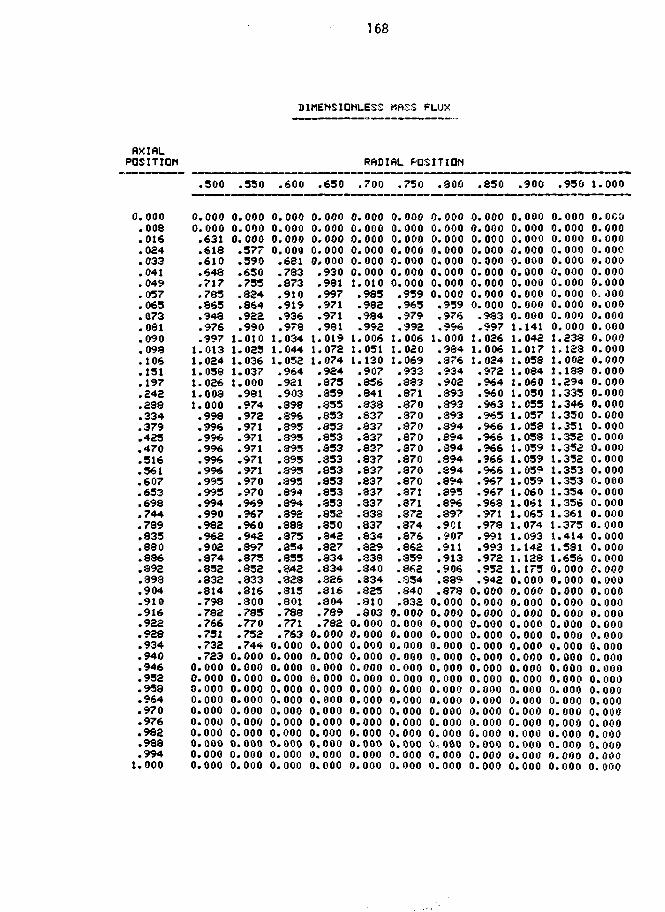
168
DIMENSIDNLE3S FLUX
flXIftLPOSITION
0.000.003.016.024.033.041.049.057.065.073.081.090.098.106.131.197.242.238.334.379.423.470.516.561.607.633.698.744.789.833.880.836.892.398.904.910.916.922.928.934.940.946.952.958.964.970.976.982.988.9941.000
.300
0.0000.000.631.618.610.648.717.783.865.948.976.9971.0131.0241.0581.0261.0081.000.998.996.996.996.996.996.993.995.994.990.982.962.902.874.852.832.814.798.782.766.731.732.723
0.0000.0000.0000.0000.0000.0000.0000.0000.0000.000
.530
0.0000.0000.000.577.390.630.733.824.864.922.9901.0101.0251.0361.0371.000.931.974.972.971.971.971.971.971.970.970.969.967.960.942.397.873.852.833.316.800.785.770.732.7440.0000.0000.0000.0000.0000.0000. 0000.0000.0000.0000.000
0.
600
0090.0000.0.*m
#
m
9
m
m1.1.1.m
m
m*m
mm
m
m
#
m
m
9
m
m
m
*
#
m
m
•
0.0.0.0.0.0.0.0.0.0.0.0.
000000681783873910919936978034044052964921903398396393895393895893395894394392883375354835$42328813301788771763000000000000000000000000000000000000
m
0.0.0.0.0.
*
0
m
*
1.1.1.
.0.0.0.0.0.0.0.0.0.0.0.0.0.
650
000000000000000930981997971971981019072074924373859355853853853853353853853353853852350342327834334326316804789782000000000000000000000000000000000000000
0.0.0.0.0.0.1.
#
RftOIAL FtJSITIQN
700
000000000000000000010985932934.9921.1.1.
#
m
#
•.
0.0.0.0.0.0.0.0.0.0.0.0.0.0.
006051130907856841838S37837337837837837337337337333837334329338340334825310803000000000000000000000000000000000000000000
.730
0.0000.0000.0000.0000.0000.0000.000.939.963.979.992
1.0061.0201.069.933• 333.371.870.370.870.870.370.870.370.870.371.371.372.374.876.362.359.362.334.840.332
0.0000.0000.0000.0000.0000.0000.0000.0000.0000.0000.0000.0000.0000.0000.000
•
0.0.0.0.0.0.0.0.
*
1.
300
000000000000000000000000939976996000984376934902393893393394894394394.394#
#
#
0.0.0.0.0.0.0.0.0.0.0.0.0.
8943958963979C1907911913906389878000000000000000000000000000000000000000
0.0000.0.
000000
.850
0.0000.0000.0000.0000.3000.0000.0000.0000.000.983.997
1.0261.0061.024.972.964.960.963.963.966.966.966.966.966.967.967.963.971.978.991.993.972.932.942
0.0000.0000.0000.0000.0000.0000.0000.0000.0000.0000.0000.0000.0000.0000.0000.0000.000
.900
0.0000.0000.0000.0000.0000.0000.0000.0000.0000.0001.1411.0421.0171.0331.0841.0601.0301.0551.0371.0581.0581.0591.0591.0591.0591.0601.0611.0631.0741.0931.1421.1281.1730.0000.0000.0000.0000.0000.0000.0000.0000.0000.0000.0000. 0000. 0000.0000. 0000. 0000.0000.000
• 930
0.0000.0000.0000.0000.0000.0000.0000.0000.0000.0000.0001.2331,1231.0021.1381.2941.335.346.3501.331.3521.352.352L.3531.3331.3541.3561.3611.3751.4141.3811.6560.0000.0000.0000.0000.0000.0000.0000.0000.0000.0000.0000.0000.0000.0000.0000.0000.0000. 0000.000
1.000
0. 0C00.0000.0000.0000.0000.0000.0000. 0000.0000. 0000. 0000. 0000.0000.0000.0000.0000.0000.0000.0000.0000.0000.0000.0000.0000.0000.0000.0000. 0000. 0000.0000.0000.0000.0000.0000. 0000.0000.0000.0000.0000.0000.0000. 0000.0000.0000.0000.0000.0000.0000.0000.0000. 000

169
ftXIflL COMPONENT OF MI=ISS FLUX
ftXIRLPOSITION
0.000.008.016.024.033.041.049.037.065.073.031.090.093.106.151.197.242.233.334.379.425.470.516.561.607.653.693.744.739.835.330.386.392.398.904.910.916.922.928.934.940.946.952.958.964.970.976.982.983.994
1.000
0.000
0.0000.0000.0000.0000. 0000.0000.0000.0000.0000.000.069.265.378.406.566.301.9.1.922.921.920.919.919.919.913.918.917.914.909.398.378.347.841.832.321.809.796.730.762.743.721.697.670.641.608.572.531.484.428.334.347.342
•
0.0.0.0.0.0.0.0.0.
,m
a
m
m
m
•
#
m
m
mm
#
m
m
#
*#
*
a
9.
m
m
#
0.
050
000000000000000000000000000137165323404430599818914922921920919919919919918917914909898378347340331321309795779761742720696669640607570529482427359306000
.100
0.0000000000
a
a
•
•
a
•
m
#
m
m
a
m
0.0.
.000
.000
.000
.000
.000
.000
.000
.435
.339
.453
.500481502699363913922921920920919919919913917915909398878846839330319806792777759739717693666637604567525473424373000000
0000001
i
•
•
•
a
•
.
a
0.0.0.
.150
.000
.000
.000
.000
.000
.000
.036
.856
.631
.638
.627595614.693361914921922921919919918918918917916914909898877845337827816303739773755736714690663633601565525431443000000000
000001
*•
•
•
a
a
a
a
a
.
m
m
m
m
a
.
.
0.0.0.0.
RftDIflL POSITION
.200
.000
.000
.000
.000
.000
.023
.991
.9578493167377608433899499359239269249239229229229219219209139129018813478353248127997357697517327X0636659630393364526494000000000000
.230
0.0000.0000.0000.000.952.9901.0081.0361.0361.0171.003.998.996.970.949.925.915.911.909.908.907.907.907.906.906.905.903.398.837.367.834.326.317.306.794.780.765.747.727.705.681.655.627.596.563.335
0.0000.0000.0000.0000.000
000
11111
4
a
•
•
a
a
a
a
a
m
a
m
m
#
a
0.0.0.0.0.0.
.300
.000
.000
.000
.660
.342
.956
.954
.998
.057
.076
.076
.061
.015
.988
.927
.901
.839
.334
.332881330330880379379378876872362342312313308301790776761743723701677651623593569000000000000000000
0
111
t
.350
.000
.161
.317
.475
.631
.773
.397
.939
.976
.999
.011
. 013
.006
.996
.925
.997
.384
.873
.875
.874
.373
.873
.873
.873
.873
.872870366336336805310807.800
•
a
a
m
a
m
0.0.0.0.0.0.0.
738774758739719696672647620597000000000000000000000
0
11
a
a
t
4
•
a
a
a
0.0.0.0.0.0.0.0.
.400
.000
.452
.479
.470
.523
.621
.733
.903
.939
.968
.987
.993
.003
.003
.963
.S4i
.925
.913
.915
.914
.914
.914
.913
.913
.913
.912
.911
.907
.897
.376833828313306791773736736715692668643622000000000000000000000000
0
1111
.a
a
a
m
.430
.000
.607
.387
.566
.569
.603
.631
.313
.919
.950
.975
.992
.004
.012
.030
.001
.934
.976
.974
.972
.972
.972
.972
.972
.971
.971
.969
.965
.936
.934
.376854834314795775734733711688664.6430.0.0.0.0.0.0.0.0.
000000000000000000000000000
00
111111
a
a
a
•
a
•
a
m
m9
0.0.0.0.0.0.0.0.0.0.
.500
.000
.000
.546
.541
.547
.376
.637
.724
.846
.943
.973
.995
.Oti
.023
.053
.026
.008
.000
.998
.996
.996
.996
.996
.996
.995
.995
.994
.990
.982960896865839815793772751729707684666000000000000000000000000000000

w 10 ro ~*a>roff©
o o oo0* co i
ooo
OO O OOO 0 OOOOOO OOOOO
oeooeoeoolilU(llNiltooW4iU(llllllUUUMa(llOliJl
o o o o o o o o o ooo o o . . . . . . .
ooooooooooooooo ooooooo
=000000000000000 ooooooooO O OiO OOOOOOOOOOOOCOCOOJOCiC9>il<i>OOOCICO(»<B«)<»0[>Q5<lD®<»<*«flCO>f>>4><il(OCOoOOOOOOO
oooooooo
oooooooo
o o o o*»OOOOO ooooo
l " ~ oooooo<*>*>i>ooUUUIUIMUroOO
oooooooooooooooooooooooooooooooooooo
ooooooooo
oooooooo
o o o o o o o o <)iub>d»or>*uwroruro
> o o oo o
>o oo o o o o <>ooooooooo<
OOOOO Ooooooooooooo
- oooooooo
oooooooo
a x
u ?
I?on
am
a•n

171
RftDIftL COMPONENT OF MftSS FLUX
AXIALPOSITION RRDIftL POSITION
0.000 .050 .100 .150 .200 .250 .300 .350 .400 .450 .500
0.000 0.000 0.000 0.000 0.000 0.000 0.000 0.000 0.000 0.000 0.000 0.000.008 0.000 0.000 0.000 0.000 0.000 0.000 0.000 - . 2 2 7 - . 4 8 1 - . 3 5 0 0.000.016 0.000 0.000 0.000 0.000 0.000 0.000 0.000 - . 4 2 1 - . 4 7 7 - . 3 3 6 - . 3 1 5.024 0.000 0.000 0.000 0.000 0.000 0.000 .177 - . 3 4 7 - . 4 0 8 - . 3 4 6 - . 2 9 9.033 0.000 0.000 0.000 0.000 0.000 .550 .252 - . 0 6 9 - . 2 6 3 - . 2 8 7 - . 2 7 0.041 0.000 0.000 0.000 0.000 .593 .300 .333 .190 - . 1 5 3 - . 2 4 4 - . 2 9 7.049 0.000 0.000 0.000 .628 .594 .439 .330 .266 - . 0 0 3 - . 2 2 7 - . 3 3 0.037 0.000 0.000 0.000 .434 .467 .437 .271 .174 .084 - . 1 0 5 - . 3 0 3.063 0.000 0.000 - . 1 1 9 .201 .223 .316 .175 .109 .040 - . 0 1 3 - . 1 8 1.073 0.000 - . 0 1 3 - . 0 3 0 - . 0 2 5 .054 .111 .084 .052 .010 - . 0 3 4 - . 0 8 0.081 0.000 - . 0 1 5 - .161 - .168 - . 0 2 3 - . 0 2 4 .011 .006 - . 0 1 3 - . 0 4 2 - . 0 7 7.090 0.000 - . 1 2 7 - . 2 0 7 - . 0 7 4 - . 0 8 7 - . 1 6 3 - . 0 4 7 - . 0 2 7 - . 0 2 8 - . 0 4 3 - . 0 6 9.098 0.000 - . 1 3 6 - . 0 9 3 - . 0 3 3 - . 1 8 0 - . 2 1 2 - . 0 7 9 - . 0 4 4 - . 0 3 4 - . 0 4 2 - . 0 5 9.106 0.000 - . 0 9 5 - . 0 4 7 - .085 - . 2 1 9 - . 1 6 6 - . 0 8 2 - . 0 4 5 - . 0 3 0 - . 0 3 4 - . 0 4 7.131 0.000 - . 0 2 7 - . 0 6 0 - .085 - . 0 8 0 - . 0 6 2 - . 0 4 2 - . 0 2 1 - . 0 0 5 .001 - . 0 0 1.197 0.000 - . 0 2 2 - . 0 4 9 - . 0 3 2 - . 0 3 8 - . 0 2 6 - . 0 1 7 - . 0 0 9 - . 0 0 1 .003 .012.242 0.000 - . 0 1 0 - . 0 1 6 - . 014 - . 0 1 0 - . 0 0 6 - . 0 0 3 .000 .003 .006 .009.238 0.000 - . 001 - . 0 0 1 - .001 - . 0 0 0 .000 .001 .002 .003 .004 .005.334 0.000 .000 .000 .000 .001 .001 .001 .002 .002 .002 .003.379 0.000 .000 .000 .000 .001 .001 .001 .001 .001 .001 .001.423 0.000 .000 .000 .000 .000 .000 .000 .001 .001 .001 .001.470 0.000 .000 .000 .000 .000 .000 .000 .000 .000 .000 .000.516 0.000 .000 .000 .000 .000 .000 .000 .000 .000 .000 .000.561 0.000 .000 .000 .000 .000 .000 .000 .000 .000.607 0.000 .000 .000 .000 .001 .001 .001 .001 .001.653 0.000 .000 .001 .001 .001 .001 .002 .002 .002.698 0.000 .001 .001 .002 .003 .003 .004 .004 .004.744 0.000 .001 .003 .004 .005 .006 .008 .009 .010.789 0.000 .002 .003 .007 .010 .013 .013 .017 .020.335 0.000 .004 .008 .012 .017 .022 .026 .029 .034.380 0.000 .003 .016 .025 .035 .056 .G34 .041 .027.886 0.000 .009 .019 .030 .042 .062 .064 .053 .044.892 0.000 .012 .023 .036 .050 .067 .074 .074 .077.398 0.000 .013 .027 .042 .056 .072 .033 .090 .102.904 0.000 .015 .031 .047 .063 .030 .094 .107 .124.910 0.000 .017 .033 .053 .071 .039 .106 .123 .144.916 0.000 .020 .039 .039 .080 .100 .119 .140 .162.922 0.000 .022 .044 .066 .039 .111 .133 .156 .130.923 0.000 .024 .049 .074 .093 .123 .147 .172 .199.934 0.000 .027 .054 .031 .109 .135 .162 .189 .217.940 0.000 .030 .060 .090 .120 .149 .173 .207 .236.946 0.000 .033 .066 .099 .132 .164 .195 .225 .244- .274 0.000.952 0.000 .036 .073 .110 .146 ,130 .213 .234 .264 0.000 0.000.958 0.000 .039 .081 .122 .161 .197 .223 .254 0.000 0.000 0.000.964 0.000 .043 .091 .136 .173 .210 .241 0.000 0.000 0.000 0.000.970 0.000 .046 .103 .154 .193 .227 0.000 0.000 0.000 0.000 0.000.976 0.000 .050 .120 .172 .210 0.000 0.000 0.000 0.000 0.000 0.000.982 0.000 .055 .142 .188 0.000 0.000 0.000 0.000 0.000 0.000 0.000.988 0.000 .058 .159 0.000 0.000 0.000 0.000 0.000 0.000 0.000 0.000.994 0.000 .130 0.000 0.000 0.000 0.000 0.000 0.000 0.000 0.000 0.000
1.000 0.000 0.000 0.000 0.000 0.000 0.000 0.000 0.000 0.000 0.000 0.000
.000
.001
.002
.005
.011
.022
.041
.05*
.074
.104
.123
.150
.170
.189
.203
.226
.245
.253
.000
.001
.002
.005
.011
.025
.050
.110
.127
.147
.165
.133
.201
.218
.236
.255
.262
.233

172
PftDZftL COMPONENT DF MASS FLUX
POSITION RADIfiL POSITION
.300 .530 .600 .650 .700 .730 .300 .830 .900 .950 1.000
0.000 0.000 0.000 0.000 0.000 0.000 0.000 0.000 0.000 0.000 0.000 0.000.008 0.000 0.000 0.000 0.000 0.000 0.000 0.000 0.000 0.000 0.000 0.000.016 -.315 0.000 0.000 0.000 0.000 0.000 0.000 0.000 0.000 0.000 0.000.024 -.299 -.233 0.000 0.000 0.000 0.000 0.000 0.000 0.000 0.000 0.000.033 -.270 -.290 -.340 0.000 0.000 0.000 0.000 0.000 0.000 0.000 0.000.041 -.297 -.342 -.431 -.463 0.000 0.000 0.000 0.000 0.000 0.000 0.000.049 -.330 -.413 -.323 -.324 -.303 0.000 0.000 0.000 0.000 0.000 0.000.057 -.303 -.416 -.300 -.530 -.473 -.430 0.000 0.000 0.000 0.000 0.000.063 -.181 -.361 -.439 -.453 -.423 -.446 -.480 0.000 0.000 0.000 0.000.073 -.080 -.228 -.382 -.417 -.406 -.404 -.445 -.492 0.000 0-000 0.000.081 -.077 -.114 -.242 -.374 -.394 -.393 -.400 -.449 -.570 0.000 0.000.090 -.069 -.097 -.119 -.230 -.361 -.392 -.364 -.363 -.483 -.320 0.000.098 -.039 -.078 -.093 -.102 -.209 -.393 -.339 -.189 -.406 -.302 0.000.106 -.047 -.062 -.072 -.072 -.061 -.313 -.270 -.034 -.332 -.235 0.000.131 -.001 -.001 .009 .036 .063 .110 .097 .073 .104 .054 0.000.197 .012 .019 .026 .033 .040 .047 .052 .052 .043 .055 0.000.242 .009 .012 .013 .017 .019 .020 .020 .020 .017 .019 0.000.288 .003 .006 .007 .008 .008 .003 .007 .007 .003 .004 0.000.334 .003 .003 .003 .003 .003 .003 .003 .002 .002 .001 0.000.379 .001 .001 .001 .001 .001 .001 .001 .001 .001 .000 0.000.425 .001 .OQJ .001 .001 .001 .001 .000 .000 .000 .000 0.000.470 .000 .000 .000 .000 .000 .000 .000 .000 .000 .000 0.000.316 .000 .000 .000 .000 .000 .000 .000 .000 .000 .000 0.000.361 .000 .000 .000 .000 .000 .000 .000 .000 .000 .000 0.000.607 .001 .001 .001 .001 .001 .001 .001 .001 .000 .000 0.000.653 .002 .002 .002 .002 .002 .002 .002 .001 .001 .001 0.000.693 .003 .003 .005 .005 .005 .005 .004 . C<03 .002 .001 0.000.744 .011 .012 .012 .012 .012 .011 .010 .003 .006 .004 0.000.789 .025 .027 .028 .029 .023 .027 .025 .022 .017 .012 0.000.335 .050 .059 .065 .066 .067 .066 .066 .062 .058 .049 0.000.880 .110 .167 .195 .166 .175 .138 .203 .134 .324 .301 0.000.336 .127 .133 .213 .201 .209 .186 .239 .227 .403 .330 0.000.892 .147 .193 .227 .233 .242 .247 .283 .326 .439 0.000 0.000.398 .165 .203 .233 .247 .262 .231 .313 .368 0.000 0.000 0.000.904 .133 .216 .244 .263 .234 .304 .343 0.000 0.000 0.000 0.000.910 .201 .231 .233 .280 .295 .323 0.000 0.000 0.000 0.000 0.000.916 .218 .247 .273 .237 .314 0.000 0.000 0.000 0.000 0.000 0.000.922 .236 .264 .279 .305 0.000 0.000 0.000 0.000 0.000 0.000 0.000.923 .235 .270 .293 0.000 0.000 0.000 0.000 0.000 0.000 0.000 0.000.934 .262 .291 0.0*»0 0.000 0.000 0.000 0.000 0.000 0.000 0.000 0.000.940 .233 C.000 0.000 0.000 0.000 0.000 0.000 0.000 0.000 0.000 0.000.946 0.000 0.000 0.000 0.000 0.000 0.000 0.000 0.000 0.000 0.000 0.000.952 0.000 0.000 0.000 0.000 0.000 0.000 0.000 0.000 0.000 0.000 0.000.958 0.000 0.000 0.000 0.000 0.000 0.000 0.000 0.000 0.000 0.000 0.000.964 0.000 0.000 0.000 0.000 0.000 0.000 0.000 0.000 0.000 0.000 0.000.970 0.000 0.000 0.000 0.000 0.000 0.000 0.000 0.000 0.000 0.000 0.000.976 0.000 0.000 0.000 0.000 0.000 0.000 0.000 0.000 0.000 0.000 0.000.932 0.000 0.000 0.000 0.000 0.000 0.000 0.000 0.000 0.000 0.000 0.000.938 0.000 0.000 0.000 0.000 0.000 0.000 0.000 0.000 0.000 0.000 0.000.994 0.000 0.000 0.000 0.000 0.000 0.000 0.000 0.000 0.000 0.000 0.000
1.000 0.000 0.000 0.000 0.000 0.000 0.000 0.000 0.000 0.000 0.000 0.000
STREflM FUNCTION CONTOUR PLDT CRESTED
ISOBflR PLOT CREATED
RUNTIME * 39.08500 SESSION » 47.£6200STOP
•tlUS. Government Printing Office: 1979 -677-013/41
Top Related